unified model for assessing checkpointing protocols at ... · dongarra, amina guermouche, thomas...

HAL Id: hal-00908447https://hal.inria.fr/hal-00908447

Submitted on 23 Nov 2013

HAL is a multi-disciplinary open accessarchive for the deposit and dissemination of sci-entific research documents, whether they are pub-lished or not. The documents may come fromteaching and research institutions in France orabroad, or from public or private research centers.

L’archive ouverte pluridisciplinaire HAL, estdestinée au dépôt et à la diffusion de documentsscientifiques de niveau recherche, publiés ou non,émanant des établissements d’enseignement et derecherche français ou étrangers, des laboratoirespublics ou privés.

Unified Model for Assessing Checkpointing Protocols atExtreme-Scale

George Bosilca, Aurélien Bouteiller, Elisabeth Brunet, Franck Cappello, JackDongarra, Amina Guermouche, Thomas Hérault, Yves Robert, Frédéric

Vivien, Dounia Zaidouni

To cite this version:George Bosilca, Aurélien Bouteiller, Elisabeth Brunet, Franck Cappello, Jack Dongarra, et al.. Uni-fied Model for Assessing Checkpointing Protocols at Extreme-Scale. Concurrency and Computation:Practice and Experience, Wiley, 2013, 26 (17), pp.2727-2810. �10.1002/cpe.3173�. �hal-00908447�

https://hal.inria.fr/hal-00908447

https://hal.archives-ouvertes.fr

CONCURRENCY AND COMPUTATION: PRACTICE AND EXPERIENCEConcurrency Computat.: Pract. Exper. 2010; 00:1–22Published online in Wiley InterScience (www.interscience.wiley.com). DOI: 10.1002/cpe

Unified Model for Assessing Checkpointing Protocols atExtreme-Scale

George Bosilca1, Aurelien Bouteiller1, Elisabeth Brunet2, Franck Cappello3, JackDongarra1, Amina Guermouche4∗, Thomas Herault1, Yves Robert1,4, Frederic Vivien4,

and Dounia Zaidouni4

1University of Tennessee Knoxville, USA2Telecom SudParis

3INRIA & University of Illinois at Urbana Champaign, USA4Ecole Normale Superieure de Lyon & INRIA, France

SUMMARY

In this paper, we present a unified model for several well-known checkpoint/restart protocols. The proposedmodel is generic enough to encompass both extremes of the checkpoint/restart space, from coordinatedapproaches to a variety of uncoordinated checkpoint strategies (with message logging). We identify a set ofcrucial parameters, instantiate them and compare the expected efficiency of the fault tolerant protocols, for agiven application/platform pair. We then propose a detailed analysis of several scenarios, including some ofthe most powerful currently available HPC platforms, as well as anticipated Exascale designs. The results ofthis analytical comparison are corroborated by a comprehensive set of simulations. Altogether, they outlinecomparative behaviors of checkpoint strategies at very large scale, thereby providing insight that is hardlyaccessible to direct experimentation. Copyright c© 2010 John Wiley & Sons, Ltd.

Received . . .

KEY WORDS: Checkpoint/restart, coordinated checkpoint, hierarchical checkpoint with messagelogging, checkpointing waste optimization problem

1. INTRODUCTION

A significant research effort is focusing on the characteristics, features, and challenges of High

Performance Computing (HPC) systems capable of reaching the Exaflop performance mark [1, 2].

The portrayed Exascale systems will necessitate billion way parallelism, resulting not only in a

massive increase in the number of processing units (cores), but also in terms of computing nodes.

Considering the relative slopes describing the evolution of the reliability of individual components

on one side, and the evolution of the number of components on the other side, the reliability

of the entire platform is expected to decrease, due to probabilistic amplification. Executions of

large parallel applications on these systems will have to tolerate a higher degree of errors and

failures than in current systems. Preparation studies forecast that standard fault tolerance approaches

(e.g., coordinated checkpointing on parallel file system) will lead to unacceptable overheads at

Exascale. Thus, it is not surprising that improving fault tolerance techniques is one of the main

recommendations isolated by these studies [1, 2].

∗Correspondence to: Journals Production Department, John Wiley & Sons, Ltd, The Atrium, Southern Gate, Chichester,West Sussex, PO19 8SQ, UK.

Copyright c© 2010 John Wiley & Sons, Ltd.

Prepared using cpeauth.cls [Version: 2010/05/13 v3.00]

2 G. BOSILCA ET AL

In this paper we focus on techniques tolerating the effect of detected errors that prevent successful

completion of the application execution. Undetected errors, also known as silent errors, are out-of-

scope of this analysis. There are two main ways of tolerating process crashes, without undergoing

significant application code refactoring: replication and rollback recovery. An analysis of replication

feasibility for Exascale systems was presented in [3]. In this paper we focus on rollback recovery,

and more precisely on the comparison of checkpointing protocols.

There are three main families of checkpointing protocols: (i) coordinated checkpointing;

(ii) uncoordinated checkpointing with message logging; and (iii) hierarchical protocols mixing

coordinated checkpointing and message logging. The key principle in all these checkpointing

protocols is that all data and states necessary to restart the execution are regularly saved in

process checkpoints. Depending on the protocol, these checkpoints are or are not guaranteed to

form consistent recovery lines. When a failure occurs, appropriate processes rollback to their last

checkpoints and resume execution.

Each protocol family has serious drawbacks. Coordinated checkpointing and hierarchical

protocols suffer a waste in terms of computing resources, whenever living processes have to rollback

and recover from a checkpoint in order to tolerate failures. These protocols may also lead to I/O

congestion when too many processes are checkpointing at the same time. Message logging increases

memory consumption, checkpointing time, and slows down failure-free execution when messages

are logged. Our objective is to identify which protocol delivers the best performance for a given

application on a given platform. While several criteria could be considered to make such a selection,

we focus on the most widely used metric, namely, the expectation of the total parallel execution time.

Fault-tolerant protocols have different overheads in fault-free and recovery situations. These

overheads depend on many factors (type of protocols, application characteristics, system features,

etc.) that introduce complexity and limit the scope of experimental comparisons conducted in the

past [4, 5]. In this paper, we approach the fault tolerant protocol comparison from an analytical

perspective. Our objective is to provide an accurate performance model covering the most suitable

rollback recovery protocols for HPC. This model captures many optimizations proposed in the

literature, but can also be used to explore the effects of novel optimizations, and to highlight the

most critical parameters to be considered when evaluating a protocol.

The main contributions of this paper are: (1) a comprehensive model that captures many

rollback recovery protocols, including coordinated checkpoint, uncoordinated checkpoint, and the

composite hierarchical hybrids; (2) a closed-form formula for the waste of computing resources

incurred by each protocol. This formula is the key to assessing existing and new protocols, and

constitutes the first tool that can help the community to compare protocols at very large scale,

and to guide design decisions for given application/platform pairs; and (3) an instantiation of the

model on several realistic scenarios involving state-of-the-art and future Exascale platforms, thereby

providing practical insight and guidance.

This paper is organized as follows. Section 2 details the characteristics of available rollback

recovery approaches, and the tradeoff they impose on failure-free execution and recovery. We

also discuss related work in this section. In Section 3, we describe our model that unifies

coordinated rollback recovery approaches, and effectively captures coordinated, partially and totally

uncoordinated approaches as well as many of their optimizations. We then use the model to

analytically assess the performance of rollback recovery protocols. We instantiate the model with

realistic scenarios in Section 4, and we present corresponding results in Section 5. These results are

corroborated by a set of simulations (Section 6), demonstrating the accuracy of the proposed unified

analytical model. Finally, we conclude and present perspectives in Section 7.

2. BACKGROUND

2.1. Rollback Recovery Strategies

Rollback recovery addresses permanent (fail-stop) process failures, in the sense that a process

reached a state where either it cannot continue for physical reasons or it detected that the current

Copyright c© 2010 John Wiley & Sons, Ltd. Concurrency Computat.: Pract. Exper. (2010)Prepared using cpeauth.cls DOI: 10.1002/cpe

UNIFIED MODEL FOR ASSESSING CHECKPOINTING PROTOCOLS AT EXTREME-SCALE 3

state has been corrupted and further continuation of the current computation is worthless. In order

to mitigate the cost of such failures, processes periodically save their state on persistent memory

(remote node, disk, ...) by taking checkpoints. In this paper, we consider only the case of fault

tolerant protocols that provide a consistent recovery, immune to the domino effect [6]. This can be

achieved by two approaches; On one extreme, coordinating checkpoints, where after a failure, the

entire application rolls back to a known consistent global state; On the opposite extreme, message

logging, which allows for independent restart of failed processes but logs supplementary state

elements during the execution to drive a directed replay of the recovering processes. The interested

reader can refer to [6] for a comprehensive survey of message logging approaches, and to [7] for a

description of the most common algorithm for checkpoint coordination. Although the uncoordinated

nature of the restart in message logging improves recovery speed compared to the coordinated

approach (during the replay, all incoming messages are available without jitter, most emissions

are discarded and other processes can continue their progress until they need to synchronize with

replaying processes) [4], the logging of message payload incurs a communication overhead and

an increases in the size of checkpoints directly influenced by the communication intensity of the

application [8]. Recent advances in message logging [9, 10, 11] have led to composite algorithms,

called hierarchical checkpointing, capable of partial coordination of checkpoints to decrease the

cost of logging, while retaining message logging capabilities to remove the need for a global restart.

These hierarchical schemes partition the application processes in groups. Each group checkpoints

independently, but processes belonging to the same group coordinate their checkpoints and recovery.

Communications between groups continue to incur payload logging. However, because processes

belonging to a same group follow a coordinated checkpointing protocol, the payload of messages

exchanged between processes within the same group is not required to be logged.

The optimizations driving the choice of the size and shape of groups are varied. A simple

heuristic is to checkpoint as many processes as possible, simultaneously, without exceeding the

capacity of the I/O system. In this case, groups do not checkpoint in parallel. Groups can also

be formed according to hardware proximity or communication patterns. In such approaches, there

may be opportunity for several groups to checkpoint concurrently. The model we propose captures

the intricacies of all such strategies, thereby also representing both extremes, coordinated and

uncoordinated checkpointing. In Section 4, we describe the meaningful parameters to instantiate

these various protocols for a variety of platforms and applications, taking into account the overhead

of message logging, and the impact of grouping strategies.

2.2. Related work

The question of optimal period of checkpoint for sequential jobs (or parallel jobs undergoing

coordinated checkpointing) has seen many studies presenting different order of estimates: see [12,

13], and [14, 15] that consider Weibull distributions, or [16] that considers parallel jobs. This is

critical to extract the best performance of any rollback-recovery protocol. However, although we use

the same approach to find the optimal checkpoint interval, we focus our study on the comparison of

different protocols that were not captured by previous models.

The literature proposes different works [17, 18, 19, 20, 21] on the modeling of coordinated

checkpointing protocols. [22] focuses on refining failure prediction; [18] and [17] focus on the

usage of available resources: some may be kept as backup in order to replace the down ones, and

others may be even shutdown in order to decrease the failure risk or to prevent storage consumption

by saving fewer checkpoint snapshots. [21] proposes a scalability model where they evaluate the

impact of failures on application performance. A significant difference with these works lies in the

inclusion of several new parameters to refine the model.

The uncoordinated and hierarchical checkpointing have been less frequently modeled. [23]

models periodic checkpointing on fault-aware parallel tasks that do not communicate. From our

point of view, this specificity does not match the uncoordinated checkpointing with message logging

we consider. In this paper, we consistently address all the three families of checkpointing protocols:

coordinated, uncoordinated, and hierarchical ones. To the best of our knowledge, it is the first

attempt at providing a unified model for this large spectrum of protocols.


4 G. BOSILCA ET AL

3. MODEL AND ANALYTICAL ASSESSMENT

In this section, we discuss the unified model, together with the closed-form formulas for the waste

optimization problem. We start with the description of the abstract model (Section 3.1). Processors

are partitioned into G groups, where each group checkpoints independently and periodically. To help

follow the technical derivation of the waste, we start with one group (Section 3.2) before tackling

the general problem with G ≥ 1 groups (Section 3.3), first under simplified assumptions, before

tackling last the fully general model, which requires three additional parameters (payload overhead,

faster execution replay after a failure, and increase in checkpoint size due to logging). We end up

with a complicated formula that characterizes the waste of resources due to checkpointing. This

formula can be instantiated to account for checkpointing protocols, see Section 4 for examples.

Note that in all scenarios, we model the behavior of tightly coupled applications, meaning that no

computation can progress on the entire platform as long as the recovery phase of a group with a

failing processor is not completed.

3.1. Abstract model

In this section, we detail the main parameters of the model. We consider an application that executes

on ptotal processors.

Units– To avoid introducing several conversion parameters, we represent all the parameters of

the model in seconds. The failure inter-arrival times, the duration of a downtime, checkpoint, or

recovery are all expressed in seconds. Furthermore, we assume (without loss of generality) that one

work unit is executed in one second, when all processors are computing at full rate. One work-unit

may correspond to any relevant application-specific quantity. When a processor is slowed-down by

another activity related to fault-tolerance (writing checkpoints to stable storage, logging messages,

etc.), one work-unit takes longer than a second to complete.

Failures and MTBF– The platform consists of ptotal identical processors. We use the term

“processor” to indicate any individually scheduled compute resource (a core, a socket, a cluster

node, etc) so that our work is agnostic to the granularity of the platform. These processors are

subject to failures. Exponential failures are widely used for theoretical studies, while Weibull or

log-normal failures are representative of the behavior of real-world platforms [24, 25, 26, 27].

The mean time between failures of a given processor is a random variable with mean (MTBF ) µ(expressed in seconds). Given the failure distribution of one processor, it is difficult to compute,

or even approximate, the failure distribution of a platform with ptotal processors, because it is

the superposition of ptotal independent and identically distributed distributions (with a single

processor). However, there is an easy formula for the MTBF of that distribution, namely µp = µptotal

.

In our theoretical analysis, we do not assume to know the failure distribution of the platform,

except for its mean value (the MTBF). Nevertheless, consider any time-interval I = [t, t+ T ] of

length T and assume that a failure strikes during this interval. We can safely state that the probability

for the failure to strike during any sub-interval [t′, t′ +X] ⊂ I of length X is XT

. Similarly, we

state that the expectation of the time m at which the failure strikes is m = t+ T2 . Neither of

these statements rely on some specific property of the failure distribution, but instead are a direct

consequence of averaging over all possible interval starting points, that will correspond to the

beginning of checkpointing periods, and that are independent of failure dates.

Tightly-coupled application– We consider a tightly-coupled application executing on the ptotalprocessors. Inter-processor messages are exchanged throughout the computation, which can only

progress if all processors are available. When a failure strikes a processor, the application is missing

one resource for a certain period of time of length D, the downtime. Then, the application recovers

from the last checkpoint (recovery time of length R) before it re-executes the work done since that

checkpoint and up to the failure. Under a hierarchical scenario, the useful work resumes only when

the faulty group catches up with the overall state of the application at failure time. Many scientific

applications are tightly-coupled and obey such a recovery scheme. Typically, the tightly-coupled

application will be an iterative application with a global synchronization point at the end of each

iteration. However, the fact that inter-processor information is exchanged continuously or at given



synchronization steps (as in BSP-like models) is irrelevant: in steady-state mode, all processors

must be available concurrently for the execution to actually progress. While the tightly-coupled

assumption may seem very constraining, it captures the fact that processes in the application depend

on each other and exchange messages at a rate exceeding the periodicity of checkpoints, preventing

independent progress.

Blocking or non-blocking checkpoint– There are various scenarios to model the cost of

checkpointing, so we use a flexible model, with several parameters to specify. The first question is

whether checkpoints are blocking or not. On some architectures, we may have to stop executing

the application before writing to the stable storage where the checkpoint data is saved; in that

case checkpoint is fully blocking. On other architectures, checkpoint data can be saved on the fly

into a local memory before the checkpoint is sent to the stable storage, while computation can

resume progress; in that case, checkpoints can be fully overlapped with computations. To deal

with all situations, we introduce a slow-down factor α: during a checkpoint of duration C, the

work that is performed is αC work units, instead of C work-units if only computation takes place.

In other words, (1− α)C work-units are wasted due to checkpoint jitter perturbing the progress

of computation. Here, 0 ≤ α ≤ 1 is an arbitrary parameter. The case α = 0 corresponds to a fully

blocking checkpoint, while α = 1 corresponds to a fully overlapped checkpoint, and all intermediate

situations can be represented.

Periodic checkpointing strategies– For the sake of clarity and tractability, we focus on periodic

scheduling strategies where checkpoints are taken at regular intervals, after some fixed amount of

work-units have been performed. This corresponds to an infinite-length execution partitioned into

periods of duration T . Without loss of generality, we partition T into T = W + C, where W is the

amount of time where only computations take place, while C corresponds to the amount of time

where checkpoints are taken.

Let TIMEbase be the application execution time without any fault tolerance mechanism and

without failures. If we assume that TIMEFF is the execution time when checkpoints are introduced

and WASTE[FF ] is the waste due to checkpoints, TIMEbase would be equal to TIMEFF minus the

waste due to checkpoints, thus:

(1− WASTE[FF ])TIMEFF = TIMEbase (1)

With the same idea, if we assume that TIMEfinal is the time needed to complete the execution with

failures and fault tolerance techniques:

(1− WASTE[fail])TIMEfinal = TIMEFF (2)

By replacing the equation 2 in the equation 1 and if we assume that WASTE is the total waste:

(1− WASTE[FF ])(1− WASTE[fail])TIMEfinal = TIMEbase (3)

We define WASTE as being the amount of time not performing useful computations,

WASTE = (TIMEfinal − TIMEbase)/TIMEfinal (4)

Finally, we deduce the following formula for the global waste:

WASTE = 1− (1− WASTE[FF ])(1− WASTE[fail]) (5)

If not slowed down for other reasons by the fault tolerant protocol (Section 3.3), the total amount

of work units that are executed during a period of length T is thus WORK = W + αC (recall that

there is a slow-down due to the overlap). In a failure-free environment, the waste of computing

resources due to checkpointing is

WASTE[FF ] =T − WORK

T=

(1− α)C

T(6)

As expected, if α = 1 there is no overhead, but if α < 1 (actual slowdown, or even blocking if

α = 0), checkpointing comes with a price in terms of performance degradation.


6 G. BOSILCA ET AL

For the time being, we do not further quantify the length of a checkpoint, which is a function of

several parameters. Instead, we proceed with the abstract model. We envision several scenarios in

Section 4, only after setting up the formula for the waste in a general context.

Processor groups– As described above, we assume that the platform is partitioned into G groups

of the same size. Each group contains q processors, hence ptotal = Gq. When G = 1, we speak of a

coordinated scenario, and we simply write C, D and R for the duration of a checkpoint, downtime

and recovery. When G ≥ 1, we speak of a hierarchical scenario. Each group of q processors

checkpoints independently and sequentially in time C(q). Similarly, we use D(q) and R(q) for

the durations of the downtime and recovery. Of course, if we set G = 1 in the (more general)

hierarchical scenario, we retrieve the value of the waste for the coordinated scenario. As already

mentioned, we derive a general expression for the waste for both scenarios, before further specifying

the values of C(q), D(q), and R(q) as a function of q and the various architectural parameters under

study.

3.2. Waste for the coordinated scenario (G = 1)

The goal of this section is to quantify the expected waste in the coordinated scenario where G = 1.

The waste is the fraction of time that the processors do not compute at full rate, either because they

are checkpointing, or because they are recovering from a failure. Recall that we write C, D, and

R for the checkpoint, downtime, and recovery using a single group of ptotal processors. We obtain

the following equation for the waste, which we explain briefly below explanation is available to the

reader and illustrate with Figure 1:

(a)

∆

αC CT − CRDTlost

P2

P1

P0

P3

Time spent checkpointingTime spent working Time spent working with slowdown

Re-executing slowed-down workRecovery timeDowntime

T

Time

(b)

∆

CT − CαCRDTlostT − C

T

P3

P0

P1

P2

Time spent checkpointingTime spent working Time spent working with slowdown

Re-executing slowed-down workRecovery timeDowntime Time

Figure 1. Coordinated checkpoint: illustrating the waste when a failure occurs (a) during the work phase;and (b) during the checkpoint phase.

WASTE[FF ] =(1− α)C

T(7)

WASTE[fail] =1

µp

(

R+D + (8)

T − C

T

[

αC +T − C

2

]

(9)

+C

T

[

αC + T − C +C

2

])

(10)



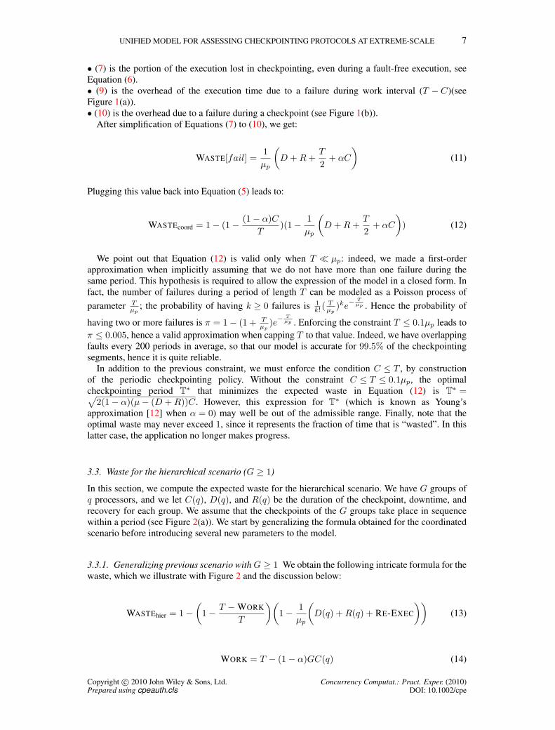
• (7) is the portion of the execution lost in checkpointing, even during a fault-free execution, see

Equation (6).

• (9) is the overhead of the execution time due to a failure during work interval (T − C)(see

Figure 1(a)).

• (10) is the overhead due to a failure during a checkpoint (see Figure 1(b)).

After simplification of Equations (7) to (10), we get:

WASTE[fail] =1

µp

(

D +R+T

2+ αC

)

(11)

Plugging this value back into Equation (5) leads to:

WASTEcoord = 1− (1−(1− α)C

T)(1−

1

µp

(

D +R+T

2+ αC

)

) (12)

We point out that Equation (12) is valid only when T ≪ µp: indeed, we made a first-order

approximation when implicitly assuming that we do not have more than one failure during the

same period. This hypothesis is required to allow the expression of the model in a closed form. In

fact, the number of failures during a period of length T can be modeled as a Poisson process of

parameter Tµp

; the probability of having k ≥ 0 failures is 1k! (

Tµp

)ke−

Tµp . Hence the probability of

having two or more failures is π = 1− (1 + Tµp

)e−

Tµp . Enforcing the constraint T ≤ 0.1µp leads to

π ≤ 0.005, hence a valid approximation when capping T to that value. Indeed, we have overlapping

faults every 200 periods in average, so that our model is accurate for 99.5% of the checkpointing

segments, hence it is quite reliable.

In addition to the previous constraint, we must enforce the condition C ≤ T , by construction

of the periodic checkpointing policy. Without the constraint C ≤ T ≤ 0.1µp, the optimal

checkpointing period T∗ that minimizes the expected waste in Equation (12) is T

∗ =√

2(1− α)(µ− (D +R))C. However, this expression for T∗ (which is known as Young’s

approximation [12] when α = 0) may well be out of the admissible range. Finally, note that the

optimal waste may never exceed 1, since it represents the fraction of time that is “wasted”. In this

latter case, the application no longer makes progress.

3.3. Waste for the hierarchical scenario (G ≥ 1)

In this section, we compute the expected waste for the hierarchical scenario. We have G groups of

q processors, and we let C(q), D(q), and R(q) be the duration of the checkpoint, downtime, and

recovery for each group. We assume that the checkpoints of the G groups take place in sequence

within a period (see Figure 2(a)). We start by generalizing the formula obtained for the coordinated

scenario before introducing several new parameters to the model.

3.3.1. Generalizing previous scenario with G ≥ 1 We obtain the following intricate formula for the

waste, which we illustrate with Figure 2 and the discussion below:

WASTEhier = 1−

(

1−T − WORK

T

)(

1−1

µp

(

D(q) +R(q) + RE-EXEC

))

(13)

WORK = T − (1− α)GC(q) (14)


8 G. BOSILCA ET AL

RE-EXEC =

T−GC(q)

T

1

G

G∑

g=1

[

(G−g+1)αC(q) +T−GC(q)

2

]

(15)

+GC(q)

T

1

G2

G∑

g=1

[

(16)

g−2∑

s=0

(G− g + s+ 2)αC(q) + T −GC(q) (17)

+GαC(q) + T −GC(q) +C(q)

2(18)

+

G−g∑

s=1

(s+ 1)αC(q)

]

(19)

• The first term in Equation (13) represents the overhead due to checkpointing during a fault-free

execution (same reasoning as in Equation (6)), and the second term the overhead incurred in case of

failure.

• (14) provides the amount of work units executed within a period of length T .

• (15) represents the time needed for re-executing the work when the failure happens in a work-only

area, i.e., during the first T −GC(q) seconds of the period (see Figure 2(a)).

• (16) deals with the case where the fault happens during a checkpoint, i.e. during the last GC(q)seconds of the period (hence the first term that represents the probability of this event). We

distinguish three cases, depending upon what group was checkpointing at the time of the failure:

- (17) is for the case when the fault happens before the checkpoint of group g (see Figure 2(b)).

- (18) is for the case when the fault happens during the checkpoint of group g (see Figure 2(c)).

- (19) is the case when the fault happens after the checkpoint of group g, during the checkpoint of

group g + s, where g + 1 ≤ g + s ≤ G (See Figure 2(d)).

Of course this expression reduces to Equation (12) when G = 1. Just as for the coordinated

scenario, we enforce the constraint

GC(q) ≤ T ≤ 0.1µp (20)

The first condition is by construction of the periodic checkpointing policy, and the second is to

enforce the validity of the first-order approximation (at most one failure per period).

3.3.2. Refining the model We introduce three new parameters to refine the model when the

processors have been partitioned into several groups. These parameters are related to the impact

of message logging on execution, re-execution, and checkpoint image size, respectively.

Impact of message logging on execution and re-execution– With several groups, inter-group

messages need to be stored in local memory as the execution progresses, and event logs must

be stored in reliable storage, so that the recovery of a given group, after a failure, can be done

independently of the other groups. This induces an overhead, which we express as a slowdown of

the execution rate: instead of executing one work-unit per second, the application executes only

λ work-units, where 0 < λ < 1. Typical values for λ are said to be λ ≈ 0.98, meaning that the

overhead due to payload messages is only a small percentage [10, 28].

On the contrary, message logging has a positive effect on re-execution after a failure, because

inter-group messages are stored in memory and directly accessible after the recovery. Our model

accounts for this by introducing a speed-up factor ρ during the re-execution. Typical values for

ρ lie in the interval [1; 2], meaning that re-execution time can be reduced by up to half for some

applications [4].

Fortunately, the introduction of λ and ρ is not difficult to account for in the expression of the

expected waste: in Equation (13), we replace WORK by λWORK and RE-EXEC by RE-EXEC

ρand



(a)

T

α(G−g+1)C

RD G.C

T−G.C−Tlost

TlostTlost

G2

G4

Gg

G1

G5


Work time Checkpoint time Work time with slowdown

Time

(b)

∆

α(s.C + Tlost)

R (G−s−1)Cα(C − Tlost)

T −G.C(G−g+1)C

α(G−g+1)C

D

C − Tlost

Tlost

s.CT −G.C

G2

Gg

G3

G1

G5



Time

(c)

∆

α(g − 1)C

(G−g)C

C − Tlost

TlostT −G.Cα(G−g+1)CRD

Tlost

(g − 1)C(G−g+1)C T −G.C

G2

Gg

G3

G5

G1



Time

(d)

∆

(g − 1)C

(G− s− g)C

α(C−Tlost)α(s.C + Tlost)

RDC − Tlost

s.C TlostT −G.C

Gg

G4

G3

G1

G5


Work time with slowdownWork time Checkpoint time

Time

Figure 2. Hierarchical checkpoint: illustrating the waste when a failure occurs (a) during the work phase(Equation (15)); and during the checkpoint phase (Equations (16)–(19)), with three sub-cases: (b) beforethe checkpoint of the failing group (Equation (17)), (c) during the checkpoint of the failing group

(Equation (18)), or (d) after the checkpoint of the failing group (Equation (19)).

obtain

WASTEhier = 1−

(

1−T − λWORK

T

)(

1−1

µp

(

D(q) +R(q) +RE-EXEC

ρ

))

(21)


10 G. BOSILCA ET AL

where the values of WORK and RE-EXEC are unchanged, and given by Equations (14) and (15 – 19)

respectively.

Impact of message logging on checkpoint size– Message logging has an impact on the execution

and re-execution rates, but also on the size of the checkpoint. Because inter-group messages are

logged, the size of the checkpoint increases with the amount of work per unit. Consider the

hierarchical scenario with G groups of q processors. Without message logging, the checkpoint time

of each group is C0(q), and to account for the increase in checkpoint size due to message logging,

we write the equation

C(q) = C0(q)(1 + βλWORK) ⇔ β =C(q)− C0(q)

C0(q)λWORK(22)

As before, λWORK = λ(T − (1− α)GC(q)) (see Equation (14)) is the number of work units, or

application iterations, completed during the period of duration T , and the parameter β quantifies

the increase in the checkpoint image size per work unit, as a proportion of the application footprint.

Typical values of β are given in the examples of Section 4. Combining with Equation (22), we derive

the value of C(q) as

C(q) =C0(q)(1 + βλT )

1 +GC0(q)βλ(1− α)(23)

The first constraint in Equation (20), namely GC(q) ≤ T , now translates intoGC0(q)(1+βλT )

1+GC0(q)βλ(1−α) ≤

T , hence

GC0(q)βλα ≤ 1 and T ≥GC0(q)

1−GC0(q)βλα(24)

4. CASE STUDIES

In this section, we use the previous model to evaluate different case studies. We propose three

generic scenarios for the checkpoint protocols, three application examples with different values for

the parameter β, and four platform instances.

4.1. Checkpointing algorithm scenarios

COORD-IO– The first scenario considers a coordinated approach, where the duration of a

checkpoint is the time needed for the ptotal processors to write the memory footprint of the

application onto stable storage. Let Mem denote this memory, and bio represents the available I/O

bandwidth. Then

C = CMem =Mem

bio

(25)

In most cases we have equal write and read speed access to stable storage, and we let R = C =CMem, but in some cases we have different values, for example with the K-Computer (see Table I).

As for the downtime, the value D is the expectation of the duration of the downtime. With a

single processor, the downtime has a constant value, but with several processors, the duration of the

downtime is difficult to compute: a processor can fail while another one is down, thereby leading to

cascading downtimes. The exact value of the downtime with several processors is unknown, even

for failures distributed according to an exponential law; but in most practical cases, the lower bound

given by the downtime of a single processor is expected to be very accurate, and we use a constant

value for D in our case studies.

HIERARCH-IO– The second scenario uses a number of relatively large groups. Typically, these

groups are composed to take advantage of the application communication pattern [10, 11]. For

instance, if the application executes on a 2D-grid of processors, a natural way to create processor

groups is to have one group per row (or column) of the grid. If all processors of a given row belong

to the same group, horizontal communications are intra-group communications and need not to be

logged. Only vertical communications are inter-group communications and need to be logged.



With large groups, there are enough processors within each group to saturate the available I/O

bandwidth, and the G groups checkpoint sequentially. Hence the total checkpoint time without

message logging, namely GC0(q), is equal to that of the coordinated approach. This leads to the

simple equation

C0(q) =CMem

G=

Mem

Gbio

(26)

where Mem denotes the memory footprint of the application, and bio the available I/O bandwidth.

Similarly as before, we use R(q) for the recovery (either equal to C(q) or not), and a constant value

D(q) = D for the downtime.

HIERARCH-PORT– The third scenario investigates the possibility of having a large number of very

small groups, a strategy proposed to take advantage of hardware proximity and failure probability

correlations [9]. However, if groups are reduced to a single processor, a single checkpointing group

is not sufficient to saturate the available I/O bandwidth. In this strategy, multiple groups of qprocessors are allowed to checkpoint simultaneously in order to saturate the I/O bandwidth. We

define qmin as the smallest value such that qminbport ≥ bio, where bport is the network bandwidth

of a single processor. In other words, qmin is the minimal size of groups so that Equation (26) holds.

Small groups typically imply logging more messages (hence a larger growth factor of the

checkpoint per work unit β, and possibly a larger impact on computation slowdown λ). For

an application executing on a 2D-grid of processors, twice as many communications will be

logged (assuming a symmetrical communication pattern along each grid direction). However, let

us compare recovery times in the HIERARCH-PORT and HIERARCH-IO strategies; assume that

R0(q) = C0(q) for simplicity. In both cases Equation (26) holds, but the number of groups is

significantly larger for HIERARCH-PORT, thereby ensuring a much shorter recovery time.

4.2. Application examples

We study the increase in checkpoint size due to message logging by detailing three application

examples that are typical scientific applications executing on 2D-or 3D-processor grids, but that

exhibit a different checkpoint increase rate parameter β.

2D-STENCIL– We first consider a 2D-stencil computation: a real matrix of size n× n is partitioned

across a p× p processor grid, where p2 = ptotal. At each iteration, each element is averaged with

its 8 closest neighbors, requiring rows and columns that lie at the boundary of the partition to be

exchanged (it is easy to generalize to larger update masks). Each processor holds a matrix block of

size b = n/p, and sends four messages of size b (one in each grid direction) . Then each element

is updated, at the cost of 9 double floating-point operations. The (parallel) work for one iteration is

thus WORK = 9b2

sp, where sp is the speed of one processor.

Here Mem = 8n2 (in bytes), since there is a single (double real) matrix to store. As already

mentioned, a natural (application-aware) group partition is with one group per row (or column)

of the grid, which leads to G = q = p. Such large groups correspond to the HIERARCH-IO

scenario, with C0(q) =CMem

G. At each iteration, vertical (inter-group) communications are logged,

but horizontal (intra-group) communications are not logged. The size of logged messages is thus

2pb = 2n for each group. If we checkpoint after each iteration, C(q)− C0(q) =2nbio

, and we derive

from Equation (22) that β =2npspn29b2 =

2sp9b3 . We stress that the value of β is unchanged if groups

checkpoint every k iterations, because both C(q)− C0(q) and WORK are multiplied by a factor k.

Finally, if we use small groups of size qmin, we have the HIERARCH-PORT scenario. We still have

C0(q) =CMem

G, but now the value of β has doubled since we log twice as many communications.

MATRIX-PRODUCT– Consider now a typical linear-algebra kernel involving matrix products. For

each matrix-product, there are three matrices involved, so Mem = 24n2 (in bytes). The matrix

partition is similar to previous scenario, but now each processor holds three matrix blocks of size

b = n/p. Consider Cannon’s algorithm [29] which has p steps to compute a product. At each step,

each processor shifts one block vertically and one block horizontally, and WORK = 2b3

sp. In the

HIERARCH-IO scenario with one group per grid row, only vertical messages are logged: β =sp6b3 .


12 G. BOSILCA ET AL

Again, β is unchanged if groups checkpoint every k steps, or every matrix product (k = p). In the

COORD-PORT scenario with groups of size qmin, the value of β is doubled.

3D-STENCIL– This application is similar to 2D-STENCIL, but with a 3D matrix of size n partitioned

across a 3D-grid of size p, where 8n3 = Mem and p3 = ptotal. Each processor holds a cube of size

b = n/p. At each iteration, each pixel is averaged with its 26 closest neighbors, and WORK = 27b3

sp.

Each processor sends the six faces of its cube, one in each direction. In addition to COORD-IO, there

are now three hierarchical scenarios: A) HIERARCH-IO-PLANE where groups are horizontal planes,

of size p2. Only vertical communications are logged, which represents two faces per processor: β =2sp27b3 ; B) HIERARCH-IO-LINE where groups are lines, of size p. Twice as many communications

are logged, which represents four faces per processor: β =4sp27b3 ; C) HIERARCH-PORT (groups of

size qmin). All communications are logged, which represents six faces per processor: β =6sp27b3 . The

order of magnitude of b is the cubic root of the memory per processor for 3D-STENCIL, while it

was its square root for 2D-STENCIL and MATRIX-PRODUCT, so β will be larger for 3D-STENCIL.

4.3. Platforms and parameters

We consider multiple platforms, existing or envisioned, that represent state-of-the-art targets

for HPC applications. Table I presents the basic characteristics of the platforms we consider.

The machine named Titan represents the fifth phase of the Jaguar supercomputer, as

presented by the Oak Ridge Leadership Computing Facility (http://www.olcf.ornl.gov/

computing-resources/titan/). The cumulated bandwidth of the I/O network is targeted

to top out at 1 MB/s/core, resulting in 300GB/s for the whole system. We consider that all existing

machines are limited for a single node output by the bus capacity, at approximately 20GB/s. The

K-Computer machine, hosted by Riken in Japan, is the second fastest supercomputer of the Top 500

list at the time of writing. Its I/O characteristics are those presented during the Lustre File System

User’s Group meeting, in April, 2011 [30], with the same bus limitation for a single node maximal

bandwidth. The two Exascale machines represent the two most likely scenarios envisioned by the

International Exascale Software Project community [1], the largest variation being on the number

of cores a single node should host. For all platforms, we let the speed of one core be 1 Gigaflops,

and we derive the speed of one processor sp by multiplying by the number of cores.

Table I also presents key parameters for all platform/scenario combinations. In all instances, we

use the default values: ρ = 1.5, λ = 0.98 and α = 0.3. These values lead to results representative of

the trends observed throughout the set of tested values.

4.4. Checkpoint duration

The last parameter that we consider is the duration of the checkpoint. Equation (25) states that

C = CMem = Membio

, hence the duration of the checkpoint is proportional to the volume of data written

to stable storage, and inversely proportional to the cumulated I/O bandwidth that is available on

the platform. As for the volume of data written, it can range from the entire memory available

on the platform (for those applications whose footprint is maximal), down to a small percentage

of this value. As for the cumulated I/O bandwidth, it can range from the values given in Table I

down to a small fraction of these values, if one can use advanced checkpointing techniques, like

incremental checkpointing [31, 32] to reduce the checkpoint size, or multi-level checkpointing [33],

diskless checkpointing [34, 35], or new generation hardware, providing local remanent memory [36]

to increase the I/O bandwidth. To account for the wide range of both parameters (volume and

bandwidth), we propose several scenarios:

Cmax In this scenario, which represents the worst case, the duration of a checkpoint is Cmax = C =CMem as in Equation (25): here we use the values of Table I, both for Mem (the application

uses the entire platform memory, and no technique such as incremental checkpointing, or

compressive checkpointing, can be used to reduce the amount of memory that needs to be

saved), and for bio (the checkpoint is stored in the remote reliable file storage system, and its

transfer speed is limited by the I/O bandwidth of the platform);


http://www.olcf.ornl.gov/computing-resources/titan/

http://www.olcf.ornl.gov/computing-resources/titan/


Cmax

XIn these scenarios, the duration of a checkpoint is Cmax

X, where X ∈ {10, 100, 1000}. Note that

this does not mean that a single technique allows to reduce the data volume by a factor X;

instead, the ratio Membio

is divided by X , by combining all available techniques and hardware,

and both the numerator (smaller volume) and the denominator (faster transfer) can contribute

to the reduction of checkpoint duration. The objective is to investigate whether, and to what

extent, faster checkpointing can prove useful, or necessary, at very large scale.

5. RESULTS FROM THE MODEL

This section covers the results of our unified model on the previously described scenarios. In

order to grant fellow researchers access to the model, results and scenarios proposed in this paper,

we made our computation spreadsheet available at http://icl.cs.utk.edu/˜herault/

UnifiedModel/.

We start with some words of caution. First, the applications used for this evaluation exhibit

properties that makes them a difficult case for hierarchical checkpoint/restart techniques. These

applications are communication intensive, which leads to a noticeable impact on performance (due

to message logging). In addition, their communication patterns create logical barriers that make

them tightly-coupled, giving a relative advantage to all coordinated checkpointing methods (due to

the lack of independent progress). However, these applications are more representative of typical

HPC applications than loosely-coupled (or even independent) jobs, and their communication-to-

computation ratio tends to zero with the problem size (full weak scalability). Next, we point out that

the theoretical values used in the model instances, and summarized in Table I, are overly optimistic,

based on the values released by the constructors and not on measured values. Finally, we stress that

the horizontal axis of all figures is the processor MTBF µ, which ranges from 1 year to 100 years, a

choice consistent with the usual representation in the community.

Section 4 above presented in detail how the values of Table I were obtained. We started with

the basic numbers of the different platforms (number of cores, processors, amount of memory and

I/O capacity), and derived for each platform and Scenario the corresponding number of groups (for

hierarchical protcols), their size, and from this the costs of taking a group checkpoint. We then

derived, for each target application, the value of β, which depends on the group size.

The first observation is that when C = Cmax, only Titan is a useful platform! Indeed, we obtain

a waste equal to 1 for all scenario/application combinations, throughout the whole range of the

MTBF µ, for both the K-Computer or Exascale platforms. This was expected and simply shows

that for such large platforms, the checkpoint time must be significantly smaller than Cmax, the time

needed to write the entire platform memory onto stable storage.

Along the same line, we only report values for C = Cmax on Titan, for C = Cmax

10 on Titan and

the K-computer, for C = Cmax

100 on Exascale-Fat, and for C = Cmax

1,000 on Exascale-Fat and Exascale-

Slim. Unreported values correspond to situations where the checkpoint duration is too large for the

platform to be useful. A few comments apply to all platforms:

• Hierarchical protocols are very sensitive to message logging: a direct relationship between β,

and the observed waste can be seen when moving from one application to another, and even

for different protocols within the same application.

• Hierarchical protocols tend to provide better results for small MTBFs. Thus, they seem more

suitable for failure-prone platforms. While they struggle when the communication intensity

increases (the case of the 3D-Stencil), they provide limited waste for all the other cases.

• The faster the checkpointing time, the smaller the waste. This conclusion is quite expected,

but our results allow quantifying the gain.

On Titan, when using Cmax, the key factors impacting the balance between coordinated and

hierarchical protocols are the communication intensity of the applications (2D-STENCIL, MATRIX-

PRODUCT, and 3D-STENCIL), and the I/O capabilities of the system. The coordinated protocol

has a slow startup, preventing the application from progressing when the platform MTBF µp is

under a system limit directly proportional to the time required to save the coordinated checkpoint.


http://icl.cs.utk.edu/~herault/UnifiedModel/


14 G. BOSILCA ET AL

Hierarchical protocols have a faster startup. However, as the MTBF increases, the optimal interval

between checkpoints increase, and the cost of logging the messages (and the increase in checkpoint

size it implies) becomes detrimental to the hierarchical protocols (even considering the most

promising approaches). The vertical segments on the graphs correspond to cut-off values where

we enforce the condition T ≤ 0.1µp (see Equation (20)). Values of µ for which no waste is reported

correspond to configurations for which no period can satisfy Equation (20).

Moving to Cmax

10 , the same remarks can be made about the shape of the figures. Compared to

a checkpointing time of Cmax, the waste is significantly smaller, leading to a very good yield of

the platform as soon as the MTBF µ exceeds 10 years. The K-Computer shows similar behavior.

However, the waste is still important even for large MTBF values for all application scenarios. This

can be attributed to the low I/O bandwidth and high amount of total memory of the parameters used

for the K-computer, when compared to the parameters considered for the Titan setup.

Moving to Exascale platforms, the Exascale-Fat platform starts to show application progress whenCmax

100 is used. However, just like the K-Computer, the waste is still important even for large MTBF.

When checkpointing becomes ten times faster, the results are more promising. The Exascale-Slim

platform starts to be useful when using Cmax

1,000 , which corresponds to checkpointing the application

within a few seconds. Overall, Exascale-Fat leads to a smaller waste (or better resource usage) than

Exascale-Slim; the main reason is that the Fat version has fewer processors, hence a larger platform

MTBF. Indeed, the individual processor MTBF is assumed to be the same for both Exascale-Fat and

Exascale-Slim, which may be unfair since there are 10 times more cores per node in the Fat version.

Setting aside the expected conclusion that an efficient process checkpointing strategy will be

critical to enable rollback/recovery at exascale, the model leads to an important prediction for

Exascale machines (Fat or Slim scenarios): unless extremely high reliability of the components can

be guaranteed (MTBF per component of 30 to 50 years for the Stencil applications), hierarchical

checkpointing approaches will (i) exhibit a lower waste than coordinated checkpointing, and (ii)

allow for an efficiency two to four times higher than replication. This conclusion holds even for

applications as tightly-coupled and as communication-intensive as the ones evaluated in this study.

6. VALIDATION OF THE MODEL

To validate the mathematical model, we wrote a simulator that generates a random trace of errors

(parameterized by an Exponential failure distribution or a Weibull one with a shape parameter of

0.7 or 0.5). On this error trace, we simulate the behavior of the various fault tolerance protocols.

In the simulator, there is no assumption on when errors can happen: an error can strike a processor

while another or the same processor is already subject to a failure and during a recovery phase.

We arbitrarily set the failure-free duration of the parallel application execution to 4 days. This

guarantees that enough failures happen during each simulation run to evaluate the waste. We

measure the simulated execution time of each application on each platform and on each error trace

using a time-out of one year: if an execution does not complete before the one year deadline, we

consider it never completes and do not report any result for this particular platform/application

setting. From the simulated execution times, we compute the average waste.

All protocols use the same parameters in the simulator as the ones fed to the mathematical model:

checkpoint durations, overheads of message logging and consequences in the checkpoint size,

amount of work that can be done in parallel, are simulated by increasing accordingly the duration

of the execution. The checkpoint interval is set in each case to the optimal value, as provided by the

mathematical model. In order to evaluate the accuracy of the optimal checkpoint interval forecasted

by the model, we also ran a set of experiments that investigate other random checkpoint interval

values around the forecasted best value, and keep the best value in the experiments denoted BestPer.

Figure 4 reports the waste for various application/platform scenarios for a Weibull failure

distribution with k = 0.7. Results for an Exponential failure distribution and for a Weibull with

k = 0.5, are provided at http://icl.cs.utk.edu/˜herault/UnifiedModel/. Each

point on the graphs is an average over 20 randomly generated instances.




Overall, Figures 3 and 4 present similar trends and conclusions. The main differences are

seen for low MTBFs, in the vicinity of cut-offs values for Figure 3. There, either the first-order

assumption could no longer be satisfied, or coordinated protocols were assessed not to allow for

any application progress. Simulations show that, in these extreme settings, our analytical study

was pessimistic: coordinated protocols have indeed very bad performance, but often applications

still make progress (albeit at unsatisfactory rate); coordinated protocols have an advantage over

hierarchical protocols for slightly lower MTBFs than predicted. However, the simulations validate

the relative performance, and the general efficiency, of the different protocols.

For each scenario and each protocol, we plot (in solid line) the average waste for the

checkpointing period computed with our model (the one minimizing Equation (21)). In Figure 4

we also plot (in dotted line) the average waste obtained for the best checkpointing period

(BestPer), numerically found by generating, and evaluating through simulations, a set of 480 periods

representative of a very large neighborhood of the period computed with our model. The very good

adequation between solid and dotted lines show that our model enables to compute near-optimal

checkpointing periods, even when its underlying assumptions cannot be guaranteed.

7. CONCLUSION

Despite the increasing importance of fault tolerance in achieving sustained, predictable

performance, the lack of models and predictive tools has restricted the analysis of fault tolerant

protocols to experimental comparisons only, which are painfully difficult to realize in a consistent

and repeated manner. This paper introduces a comprehensive model of rollback recovery protocols

that encompasses a wide range of checkpoint/restart protocols, including coordinated checkpoint

and an assortment of uncoordinated checkpoint protocols (based on message logging). This model

provides the first tool for a quantitative assessment of all these protocols. Instantiation on future

platforms enables the investigation and understanding of the behavior of fault tolerant protocols at

scales currently inaccessible. The results presented in Section 5, and corroborated by Section 6,

highlight the following tendencies:

• Hardware properties will have tremendous impact on the efficiency of future platforms. Under

the early assumptions of the projected Exascale systems, rollback recovery protocols are mostly

ineffective. In particular, significant efforts are required in terms of I/O bandwidth to enable any

type of rollback recovery to be competitive. With the appropriate provision in I/O (or the presence

of distributed storage on nodes), rollback recovery can be competitive and significantly outperform

full-scale replication [3] (which by definition cannot reach more than 50% efficiency).

• Under the assumption that I/O network provision is sufficient, the reliability of individual

processors has a minor impact on rollback recovery efficiency. This suggests that most research

efforts, funding and hardware provisions should be directed to I/O performance rather than

improving component reliability in order to increase the scientific throughout of Exascale platforms.

• The model outlines some realistic ranges where hierarchical checkpointing outperforms

coordinated checkpointing, thanks to its faster recovery from individual failures. This early result

had already been outlined experimentally at smaller scales, but it was difficult to project at future

scales. Our study provides a theoretical foundation and a quantitative evaluation of the drawbacks of

checkpoint/restart protocols at Exascale; it can be used as a first building block to drive the research

field forward, and to design platforms with specific resilience requirements.

Throughout the simulations, we have checked (by an extensive brute-force comparison)

that our model could predict near-optimal checkpointing periods for the whole range of the

protocol/platform/application combinations; this gives us very good confidence that this model will

prove reliable and accurate in other frameworks. As we are far from a comprehensive understanding

of future Exascale applications and platform characteristics, we hope that the community will be

interested in instantiating our publicly available model with different scenarios and case-studies.


16 G. BOSILCA ET AL

ACKNOWLEDGEMENTS

This work was partly supported by the French ANR White Project RESCUE, the US National

Science Foundation through award #1063019, and the US Department Of Energy Award #DE-

FG02-11ER26059. Yves Robert is with Institut Universitaire de France. We would like to thank

the reviewers for their comments and suggestions, which greatly helped improve the final version

of the paper.



Name Number of Number of Number of cores Memorycores processors ptotal per processor per processor

Titan 299,008 18,688 16 32GBK-Computer 705,024 88,128 8 16GB

Exascale-Slim 1,000,000,000 1,000,000 1,000 64GBExascale-Fat 1,000,000,000 100,000 10,000 640GB

Name I/O Network Bandwidth (bio) I/O Bandwidth (bport)Read Write Read/Write per processor

Titan 300GB/s 300GB/s 20GB/sK-Computer 150GB/s 96GB/s 20GB/s

Exascale-Slim 1TB/s 1TB/s 200GB/sExascale-Fat 1TB/s 1TB/s 400GB/s

Name Scenario G (C(q)) β for β for2D-STENCIL MATRIX-PRODUCT

COORD-IO 1 (2,048s) / /Titan HIERARCH-IO 136 (15s) 0.0001098 0.0004280

HIERARCH-PORT 1,246 (1.6s) 0.0002196 0.0008561COORD-IO 1 (14,688s) / /

K-Computer HIERARCH-IO 296 (50s) 0.0002858 0.001113HIERARCH-PORT 17,626 (0.83s) 0.0005716 0.002227

COORD-IO 1 (68,719s) / /Exascale-Slim HIERARCH-IO 1,000 (68.7s) 0.0002599 0.001013

HIERARCH-PORT 200,000 (0.32s) 0.0005199 0.002026COORD-IO 1 (68,719s) / /

Exascale-Fat HIERARCH-IO 316 (217s) 0.00008220 0.0003203HIERARCH-PORT 33,333 (1.92s) 0.00016440 0.0006407

Name Scenario G β for 3D-STENCIL

COORD-IO 1 /Titan HIERARCH-IO-PLANE 26 0.001476

HIERARCH-IO-LINE 676 0.002952HIERARCH-PORT 1,246 0.004428

COORD-IO 1 /K-Computer HIERARCH-IO-PLANE 44 0.003422

HIERARCH-IO-LINE 1,936 0.006844HIERARCH-PORT 17,626 0.010266

COORD-IO 1 /Exascale-Slim HIERARCH-IO-PLANE 100 0.003952


COORD-IO 1 /Exascale-Fat HIERARCH-IO-PLANE 46 0.001834


Table I. Basic characteristics of platforms used to instantiate the model, and all parameters for eachplatform/scenario combination. The equations C0(q) = C/G and R0(q) = R/G always hold.


18 G. BOSILCA ET AL

Tit

anC

max

Tit

anC

max

10

K-C

om

pute

rC

max

10

Exas

cale

-Fat

Cm

ax

100

Exas

cale

-Sli

mC

max

1,000

Exas

cale

-Fat

Cm

ax

1,000

2D-STENCIL MATRIX-PRODUCT 3D-STENCIL

Figure 3. Model: waste as a function MTBF µ (years per processor).



HierarchicalHierarchical-PortCoordinated

Hierarchical BestPerHierarchical-Port BestPerCoordinated BestPer

HierarchicalHierarchical-PortCoordinated

Hierarchical BestPerHierarchical-Port BestPerCoordinated BestPer

Hierarchical-PortHierarchical-PlaneHierarchical-LineCoordinated

Hierarchical-Port BestPerHierarchical-Plane BestPerHierarchical-Line BestPerCoordinated BestPer

Tit

anC

max

0

0.1

0.2

0.3

0.4

0.5

0.6

0.7

0.8

0.9

1

1 2 3 4 5 7.5 10 15 20 25 35 50 75 100

Hierarchical

Hierarchical Port

Coordinated

Hierarchical BestPer

Hierarchical Port BestPer

Coordinated BestPer

0

0.1

0.2

0.3

0.4

0.5

0.6

0.7

0.8

0.9

1

1 2 3 4 5 7.5 10 15 20 25 35 50 75 100

Hierarchical

Hierarchical Port

Coordinated

Hierarchical BestPer


Coordinated BestPer

0

0.1

0.2

0.3

0.4

0.5

0.6

0.7

0.8

0.9

1

1 2 3 4 5 7.5 10 15 20 25 35 50 75 100

Hierarchical Port

Hierarchical Plane

Hierarchical Line

Coordinated


Hierarchical Plane BestPer

Hierarchical Line BestPer

Coordinated BestPer

Tit

anC

max

10

0

0.1

0.2

0.3

0.4

0.5

0.6

0.7

0.8

0.9

1

1 2 3 4 5 7.5 10 15 20 25 35 50 75 100

0

0.1

0.2

0.3

0.4

0.5

0.6

0.7

0.8

0.9

1

1 2 3 4 5 7.5 10 15 20 25 35 50 75 100

0

0.1

0.2

0.3

0.4

0.5

0.6

0.7

0.8

0.9

1

1 2 3 4 5 7.5 10 15 20 25 35 50 75 100

K-C

om

pute

rC

max

10

0

0.1

0.2

0.3

0.4

0.5

0.6

0.7

0.8

0.9

1

1 2 3 4 5 7.5 10 15 20 25 35 50 75 100

0

0.1

0.2

0.3

0.4

0.5

0.6

0.7

0.8

0.9

1

1 2 3 4 5 7.5 10 15 20 25 35 50 75 100

0

0.1

0.2

0.3

0.4

0.5

0.6

0.7

0.8

0.9

1

1 2 3 4 5 7.5 10 15 20 25 35 50 75 100

ExaS

cale

-Fat

Cm

ax

100

0

0.1

0.2

0.3

0.4

0.5

0.6

0.7

0.8

0.9

1

1 2 3 4 5 7.5 10 15 20 25 35 50 75 100

0

0.1

0.2

0.3

0.4

0.5

0.6

0.7

0.8

0.9

1

1 2 3 4 5 7.5 10 15 20 25 35 50 75 100

0

0.1

0.2

0.3

0.4

0.5

0.6

0.7

0.8

0.9

1

1 2 3 4 5 7.5 10 15 20 25 35 50 75 100

Exas

cale

-Sli

mC

max

1,000

0

0.1

0.2

0.3

0.4

0.5

0.6

0.7

0.8

0.9

1

1 2 3 4 5 7.5 10 15 20 25 35 50 75 100

0

0.1

0.2

0.3

0.4

0.5

0.6

0.7

0.8

0.9

1

1 2 3 4 5 7.5 10 15 20 25 35 50 75 100

0

0.1

0.2

0.3

0.4

0.5

0.6

0.7

0.8

0.9

1

1 2 3 4 5 7.5 10 15 20 25 35 50 75 100

Exas

cale

-Fat

Cm

ax

1,000

0

0.1

0.2

0.3

0.4

0.5

0.6

0.7

0.8

0.9

1

1 2 3 4 5 7.5 10 15 20 25 35 50 75 100

0

0.1

0.2

0.3

0.4

0.5

0.6

0.7

0.8

0.9

1

1 2 3 4 5 7.5 10 15 20 25 35 50 75 100

0

0.1

0.2

0.3

0.4

0.5

0.6

0.7

0.8

0.9

1

1 2 3 4 5 7.5 10 15 20 25 35 50 75 100

2D-STENCIL MATRIX-PRODUCT 3D-STENCIL

Figure 4. Waste as a function of processor MTBF µ, for a Weibull distribution with k=0.7


20 G. BOSILCA ET AL



References

1. Dongarra J, Beckman P, Aerts P, Cappello F, Lippert T, Matsuoka S, Messina P, Moore T, Stevens R,Trefethen A, et al.. The international exascale software project: a call to cooperative action by the global high-performance community. Int. J. High Perform. Comput. Appl. 2009; 23(4):309–322, doi:http://dx.doi.org/10.1177/1094342009347714.

2. Sarkar V, et al.. Exascale software study: Software challenges in extreme scale systems 2009. White paperavailable at: http://users.ece.gatech.edu/mrichard/ExascaleComputingStudyReports/ECSS%20report%20101909.pdf.

3. Ferreira K, Stearley J, Laros JHI, Oldfield R, Pedretti K, Brightwell R, Riesen R, Bridges PG, Arnold D. Evaluatingthe Viability of Process Replication Reliability for Exascale Systems. Proc. ACM/IEEE Conf. on Supercomputing,2011.

4. Bouteiller A, Herault T, Krawezik G, Lemarinier P, Cappello F. MPICH-V: a multiprotocol fault tolerant MPI.IJHPCA 2006; 20(3):319–333, doi:10.1177/1094342006067469.

5. Rao S, Alvisi L, Viny HM, Sciences DC. Egida: An extensible toolkit for low-overhead fault-tolerance. InSymposium on Fault-Tolerant Computing, Press, 1999; 48–55.

6. Elnozahy ENM, Alvisi L, Wang YM, Johnson DB. A survey of rollback-recovery protocols in message-passingsystems. ACM Computing Survey 2002; 34:375–408.

7. Chandy KM, Lamport L. Distributed snapshots : Determining global states of distributed systems. Transactions onComputer Systems, vol. 3(1), ACM, 1985; 63–75.

8. Rao S, Alvisi L, Vin HM. The cost of recovery in message logging protocols. 17th Symposium on ReliableDistributed Systems (SRDS), IEEE CS Press, 1998; 10–18.

9. Bouteiller A, Herault T, Bosilca G, Dongarra JJ. Correlated set coordination in fault tolerant message loggingprotocols. Proc. of Euro-Par’11 (II), LNCS, vol. 6853, Springer, 2011; 51–64, doi:http://dx.doi.org/10.1007/978-3-642-23397-5 6.

10. Guermouche A, Ropars T, Snir M, Cappello F. HydEE: Failure Containment without Event Logging for LargeScale Send-Deterministic MPI Applications. IPDPS’12, IEEE, 2012.

11. Esteban Meneses CLM, Kale LV. Team-based message logging: Preliminary results. Workshop Resilience inClusters, Clouds, and Grids (CCGRID 2010)., 2010.

12. Young JW. A first order approximation to the optimum checkpoint interval. Comm. of the ACM 1974; 17(9):530–531.

13. Daly JT. A higher order estimate of the optimum checkpoint interval for restart dumps. FGCS 2004; 22(3):303–312.14. Ling Y, Mi J, Lin X. A variational calculus approach to optimal checkpoint placement. IEEE Trans. Computers

2001; :699–708.15. Ozaki T, Dohi T, Okamura H, Kaio N. Distribution-free checkpoint placement algorithms based on min-max

principle. IEEE TDSC 2006; :130–140.16. Bougeret M, Casanova H, Rabie M, Robert Y, Vivien F. Checkpointing strategies for parallel jobs. Proc. ACM/IEEE

Conf. on Supercomputing, 2011.17. Plank JS, Thomason MG. Processor allocation and checkpoint interval selection in cluster computing systems.

Journal of Parallel and Distributed Computing 2001; 61:1590.18. Jin H, Chen Y, Zhu H, Sun XH. Optimizing HPC Fault-Tolerant Environment: An Analytical Approach. 39th Int.

Conf. Parallel Processing (ICPP), 2010; 525 –534, doi:10.1109/ICPP.2010.80.19. Wang L, Karthik P, Kalbarczyk Z, Iyer R, Votta L, Vick C, Wood A. Modeling Coordinated Checkpointing for

Large-Scale Supercomputers. Proceedings of ICDSN’05, 2005; 812–821.20. Oldfield R, Arunagiri S, Teller P, Seelam S, Varela M, Riesen R, Roth P. Modeling the impact of checkpoints on

next-generation systems. Proceedings of IEEE MSST’07, 2007; 30 –46, doi:10.1109/MSST.2007.4367962.21. Zheng Z, Lan Z. Reliability-aware scalability models for high performance computing. Proc. of IEEE Cluster’09,

2009; 1 –9, doi:10.1109/CLUSTR.2009.5289177.22. Bouguerra MS, Trystram D, Wagner F. Complexity Analysis of Checkpoint Scheduling with Variable Costs. IEEE

Transactions on Computers 2012; 99(PrePrints), doi:http://doi.ieeecomputersociety.org/10.1109/TC.2012.57.23. Wu M, Sun XH, Jin H. Performance under failures of high-end computing. Proc. ACM/IEEE Conf. on

Supercomputing, 2007.24. Heath T, Martin RP, Nguyen TD. Improving cluster availability using workstation validation. SIGMETRICS Perf.

Eval. Rev. 2002; 30(1):217–227.25. Schroeder B, Gibson GA. A large-scale study of failures in high-performance computing systems. Proc. of DSN,

2006.26. Liu Y, Nassar R, Leangsuksun C, Naksinehaboon N, Paun M, Scott S. An optimal checkpoint/restart model for a

large scale high performance computing system. IPDPS’08, IEEE, 2008; 1–9.27. Heien E, Kondo D, Gainaru A, LaPine D, Kramer B, Cappello F. Modeling and tolerating heterogeneous failures

in large parallel systems. Proc. ACM/IEEE Conf. on Supercomputing, 2011.28. Bouteiller A, Bosilca G, Dongarra J. Redesigning the message logging model for high performance. Concurrency

and Computation: Practice and Experience 2010; 22(16):2196–2211, doi:10.1002/cpe.1589.29. Cannon LE. A cellular computer to implement the Kalman filter algorithm. PhD Thesis, Montana State University

1969.30. Sumimoto S. An Overview of Fujitsu’s Lustre Based File System. Lustre Filesystem Users’ Group Meeting,

Orlando, USA. April 2011.31. Agarwal S, Garg R, Gupta MS, Moreira JE. Adaptive incremental checkpointing for massively parallel systems.

Proceedings of the 18th annual international conference on Supercomputing, ICS ’04, ACM: New York, NY, USA,2004; 277–286, doi:10.1145/1006209.1006248.

32. Gioiosa R, Sancho JC, Jiang S, Petrini F, Davis K. Transparent, incremental checkpointing at kernel level:a foundation for fault tolerance for parallel computers. Proceedings of the 2005 ACM/IEEE conference on


http://users.ece.gatech.edu/mrichard/ExascaleComputingStudyReports/ECSS%20report%20101909.pdf

http://users.ece.gatech.edu/mrichard/ExascaleComputingStudyReports/ECSS%20report%20101909.pdf

22 G. BOSILCA ET AL

Supercomputing, SC ’05, IEEE Computer Society: Washington, DC, USA, 2005; 9–, doi:10.1109/SC.2005.76.33. Moody A, Bronevetsky G, Mohror K, Supinski BRd. Design, Modeling, and Evaluation of a Scalable Multi-level

Checkpointing System. Proceedings of the ACM/IEEE SC Conference, 2010; 1–11.34. Plank JS, Li K, Puening MA. Diskless checkpointing. IEEE Transactions on Parallel and Distributed Systems 1998;

9:972–986, doi:http://doi.ieeecomputersociety.org/10.1109/71.730527.35. Gomez LAB, Maruyama N, Cappello F, Matsuoka S. Distributed diskless checkpoint for large scale systems.

Proceedings of the 2010 10th IEEE/ACM International Conference on Cluster, Cloud and Grid Computing,CCGRID ’10, IEEE Computer Society: Washington, DC, USA, 2010; 63–72, doi:10.1109/CCGRID.2010.40.

36. Ouyang X, Marcarelli S, Panda DK. Enhancing checkpoint performance with staging io and ssd. Proceedings ofthe 2010 International Workshop on Storage Network Architecture and Parallel I/Os, SNAPI ’10, IEEE ComputerSociety: Washington, DC, USA, 2010; 13–20, doi:10.1109/SNAPI.2010.10. URL http://dx.doi.org/10.1109/SNAPI.2010.10.


http://dx.doi.org/10.1109/SNAPI.2010.10

http://dx.doi.org/10.1109/SNAPI.2010.10

unified model for assessing checkpointing protocols at ... · dongarra, amina guermouche, thomas...

Documents