unified and integrated approach in a new timoshenko beam
TRANSCRIPT

EuropEan Journal of Computational mEChaniCs, 2017Vol. 26, no. 3, 282–308https://doi.org/10.1080/17797179.2017.1328643
Unified and integrated approach in a new Timoshenko beam element
Irwan Katili
universitas indonesia, Depok, West Java, indonesia
ABSTRACTThis paper presents a new unified and integrated approach to construct locking-free finite elements for bending of shear deformable beam element. The new UI (Unified and Integrated) element, with two nodes and three degrees of freedom (d.o.f.) per node, is formulated based on a pure displacement formulation and utilises vertical displacement, rotational and curvature as three d.o.f. at the nodes. A continuity of C2 Hermite shape functions for bending deflection vb is used in which rotation function of θ and curvature of χ are dependently expressed as the first and second derivatives of bending deflection. The formulation of element takes account of the effect of shear transversal forces in order to behave appropriately in the analysis of thin and thick beams. A shear influence factor of ϕ is expressed explicitly, which is a function of length thickness ratio (L/h), as a control for shear deformation. The resulting UI element is absolutely free from locking and preserves the high accuracy of the standard locking-free finite elements and classical Bernoulli Euler element. Finally, several numerical tests are presented to confirm the performance of the proposed formulations.
1. Introduction
In beam theories, the simplest model is the Bernoulli–Euler beam (BEB) model, in which cross sections perpendicular to the neutral axis prior to bending remain plane and perpendicular to the neutral axis posterior to bending, which implies that the rotation of cross section can be obtained from the derivative of the deflec-tion. It is well known that the BEB is more suitable for slender beams and neglects shear deformation effects. By taking into account the effects of shear deformation, Timoshenko proposed a further improvement of the beam theory (Timoshenko, 1921, 1922). In the Timoshenko theory, cross sections are also assumed to remain straight but not necessarily normal to the beam axis due to shear deformability.
© 2017 informa uK limited, trading as taylor & francis Group
KEYWORDSunified and integrated approach; finite element; timoshenko beam; shear influence factor
ARTICLE HISTORYreceived 27 october 2016 accepted 7 may 2017
CONTACT irwan Katili [email protected], [email protected]
EUROPEAN JOURNAL OF COMPUTATIONAL MECHANICS 283
As consequence, rotation (θ) and deflection (v) are typically considered as inde-pendent variables.
A number of beam type finite elements based on Timoshenko theory has been discussed in literatures. Timoshenko Linear beam (TLB) element of classic dis-placement model with two nodes and two degree of freedoms, which takes into account shear deformation and is based on beam theory of Timoshenko (1921, 1922), will experience shear locking if it is applied on a thin beam (L/h > 20). Linear interpolations of total vertical displacement (v) and rotation (θ) lead to an element exhibiting overly stiff characteristic, which gives reasonable result only for the case of very thick beams. This problem can be solved using selective reduced integration proposed by Hughes, Taylor, and Kanoknukulchai (1977), stating that shear deformation is constant along the element. Two-node element with linear interpolations and selective reduced integration evinced satisfactory properties over a wide variety of length thickness ratios (L/h). Nevertheless, the convergence speed of the element is not as fast as of the classic element that neglects the shear deformation and is based on beam theory of Bernoulli–Euler. Hence, we conclude that it would be very good if we have an element of two nodes and two or three degree of freedoms per node without shear locking and has equal convergence speed as the Bernoulli–Euler element.
Another concept to solve the shear locking problem is the element called Mixed Interpolation of Tensorial Components (MITC), which is based on Assumed Natural Strain (ANS) method proposed by Bathe and Dvorkin (1985). The MITC Quadrilateral element, when applied to beam case, results in beam element which has a similarity with the beam element from the method by Hughes and Tezduyar (1981). Here, conditions for the shear strains are formulated constant along the edges of the element and the resulting discrete shear strains at the nodes are inter-polated over the element domain with standard shape functions. This method is classified as an ANS.
Another recent ANS method, called Discrete Shear Gap (DSG) element is proposed by Bletzinger, Bischoff, and Ramm (2000). The resulting element is free of locking and passes the patch test. The Quadrilateral DSG element has a certain relation to the Quadrilateral MITC element. In the case of a bilinear interpolation, they result in identical elements.
The beam element called Discrete Shear Beam (DSB), with cubic interpolations for total vertical displacement (v) and quadratic interpolations for rotation (θ), has been a basis for the development of triangular and quadrilateral plate and shell elements called DKMT and DKMQ (Katili, 1993a, 1993b, 2006; Katili, Batoz, Maknun, Hamdouni, & Millet, 2015; Katili, Maknun, Hamdouni, & Millet, 2015; Maknun, Katili, Millet, & Hamdouni, 2016).
Kiendl, Auricchio, Hughes, and Reali (2015) develop a relation between deflec-tion and rotation of Timoshenko beams for isogeometric analysis which leads to curvature and shear deformation expressions with only one variable. The ver-tical displacement (v) is split into a bending (vb) and a shear part (vs), which
284 I. KATILI
are related to each other, which allows expressing all derived variable, such as rotation, curvature and shear strain, in terms of the bending displacement (vb) as the only variable. The idea of splitting the displacement of Timoshenko beams into a bending and a shear part can be found in papers from the early days of beam finite elements, for example, Kapur (1966). Similar approaches have been presented by Li (2008) and Falsone and Settineri (2011). The strong form of the problem involves the fourth derivative of the bending displacement (vb), whereas the symmetric weak form involves third and second derivatives of the bending displacement (vb). Based on these, Kiendl et al. (2015) develop IGA-Collocation and IGA-Galerkin formulations.
This paper is meant to present the development of a new beam element called UI (Unified and Integrated) using C2 Hermite polynomial expansion at continu-ity of 5th degree for bending displacement (vb). Section 2 provides the classical Timoshenko beam theory and Section 3 provides the Unified and Integrated Approach showing the Timoshenko beam equations with bending displacement (vb) as the only variable. In Section 4–7, the formulation of BEB element and various Timoshenko beam elements (TLB, DSG, DSB) are summarised briefly. The stiffness matrix of UI element is presented in section 8 based on unified and integrated approach in the weak form which involves both second and third derivatives of the bending displacement (vb). In Section 9, performance of UI element is compared with BEB, TLB, DSG and DSB elements.
2. Classical Timoshenko beams theory
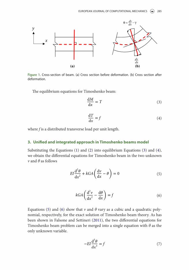
Assuming small displacement and for establishing notation, the equations of Timoshenko (1921, 1922) are first summarised. Cartesian coordinates are cho-sen such that the x-axis is oriented in the axial direction at the mid-plane of the unbent beam, and the positive y-axis is directed upwards and perpendicular to the x-axis (Figure 1). The curvature and the shear deformation are
The shear deformations γ are assumed to be uniform at any cross-sectional area and only dependent on x. We recall the constitutive equations of Timoshenko beam theory for the bending moment M and the shear force T:
where v(x) = vertical displacement; (x) = rotation of the cross section at any point x along the beam; χ(x) = curvature; (x) = shear deformation; EI = flexural rigidity; kGA = shear rigidity; E = Young’s Modulus; k = shear correction factor; G = Shear Modulus; A = cross-sectional area; I = the second moment of inertia; v(x) = vertical displacement of the beam centre line; dv
dx = gradient of the vertical
displacement with respect to x.
(1) = −d
dx; =
dv
dx−
(2)M = EI ;T = kGA
EUROPEAN JOURNAL OF COMPUTATIONAL MECHANICS 285
The equilibrium equations for Timoshenko beam:
where f is a distributed transverse load per unit length.
3. Unified and integrated approach in Timoshenko beams model
Substituting the Equations (1) and (2) into equilibrium Equations (3) and (4), we obtain the differential equations for Timoshenko beam in the two unknown v and θ as follows
Equations (5) and (6) show that v and θ vary as a cubic and a quadratic poly-nomial, respectively, for the exact solution of Timoshenko beam theory. As has been shown in Falsone and Settineri (2011), the two differential equations for Timoshenko beam problem can be merged into a single equation with θ as the only unknown variable.
(3)dM
dx= T
(4)dT
dx= f
(5)EId2
dx2+ kGA
(dv
dx−
)= 0
(6)kGA
(d2v
dx2−
d
dx
)= f
(7)−EId3
dx3= f
dv
dvdx
dx
θ = γ
(a) (b)
Figure 1. Cross-section of beam. (a) Cross section before deformation. (b) Cross section after deformation.
286 I. KATILI
By integrating Equation (5), we find the vertical displacement v as follows:
where c is an integration constant.In (Kiendl et al., 2015) Equation (8) is considered consist of two parts: first is
vb as a bending part and second is vs as a shear part, as follows
Differentiating the Equation (9) yields
Substituting (13) into curvature in Equation (1) yields
Substituting (13) into (12) and then substituting the result into shear deformation in Equation (1) yields =
dvs
dx, and from (14) we obtain
By integrating (16) we obtain
(8)v =x∫0
dx −EI
kGA
d
dx+ c
(9)v = vb + vs
(10)vb =x∫0
dx + c
(11)vs = −EI
kGA
d
dx+ c
(12)dv
dx=
dvbdx
+dvsdx
(13)dvbdx
=
(14)dvsdx
= −EI
kGA
d2
dx2= −
EI
kGA
d3vb
dx3
(15) = −d2vb
dx2
(16) =dvsdx
= −EI
kGA
d2
dx2= −
EI
kGA
d3vb
dx3
(17)vs = −EI
kGA
d2vb
dx2

EUROPEAN JOURNAL OF COMPUTATIONAL MECHANICS 287
Finally, the Equation (9) can be expressed in terms of only vb
Substituting Equation (13) into (7) gives
These differential Equations (15–19) are identical to the ones for a BEB model with v replacing vb but fully account for shear deformation. For very slender beam, EI/kGA ≈ 0, vs ≈ 0, vb ≈ v, and Equations (15–19) exactly reproduce the Bernoulli–Euler equations. The advantage lies in that all physical quantities can be expressed in terms of vb and its derivatives. The differential Equation (19) is of fourth order and four boundary conditions are necessary to complete the specification of the boundary value problem.
The boundaries of the beam are denoted by Γ = 0UL, with L is the length of beam. Furthermore, Γv, Γθ, ΓM, ΓT indicate the boundaries which prescribes v, θ, M, and T, respectively. The boundary conditions can then be formulated as follow, with barred symbols indicating the prescribed boundary values:
It is important to note that a zero vertical displacement v at boundary condition does not imply that both vb and vs are zero at the boundary, but that their sum is zero, i.e. vb + vs = 0 → vb ≠ 0, vs ≠ 0.
(18)v = vb −EI
kGA
d2vb
dx2
(19)−EId4vb
dx4= f
(20)vb −EI
kGA
d2vb
dx2= v → Γv
(21)dvbdx
= → Γ𝜃
(22)−EId2vb
dx2= ±M → ΓM
(23)−EId3vb
dx3= ±T → ΓT

288 I. KATILI
The differential Equation (19) is the strong form of fourth order and we develop a weak form by multiplying Equation (19) with a test function v* (18):
In order to obtain the weak form, we apply integration by parts separately over the domain Ω = [0, L] such that the trial and test functions appear with the same derivative order. This approach is the same with virtual work principle as follows:
The Equation (25) represents the classical equilibrium of principle of virtual work (PVW) and therefore can take the form:
The two terms on the left hand side (l.h.s) are the bending and shear parts of the internal virtual work. On the right hand side (r.h.s) are the external virtual works. The external concentrated vertical point load T and distributed loads f are taken as positive if they act in the direction of the global y axis. The external concentrated moments M acting at beam points are taken as positive if they act anticlockwise, which is consistent with the definition of the rotation.
4. BEB element
The classical Bernoulli–Euler thin beam theory is based on hypothesis that the cross-sections normal to the beam axis remain plane and orthogonal to the beam axis after deformation. This hypothesis implies that the shear deformation γ is neglected and the rotation θ is equal to the slope of the beam axis. From (1) we find:
The Equation (27) may be regarded as Bernoulli–Euler constraint. Substituting (27) into (26) gives the PVW
(24)L∫0
(v∗b −
EI
kGA
d2v∗b
dx2
)(−EI
d4vb
dx4
)dx =
L∫0
(v∗b −
EI
kGA
d2v∗b
dx2
)f dx
(25)
L∫0
d2v∗b
dx2EI
d2vb
dx2dx +
L∫0
d3v∗b
dx3(EI)2
kGA
d3vb
dx3dx =
L∫0
(v∗b −
EI
kGA
d2v∗b
dx2
)f dx −
dv∗bdx
|ΓMM
+
(v∗b −
EI
kGA
d2v∗b
dx2
)|ΓTT
(26)L∫0
𝜒∗EI𝜒dx +L∫0
𝛾∗kGA𝛾dx = fL∫0
v∗dx + (𝜃∗)|ΓMM + (v∗)|ΓT
T
(27) =dv
dx− = 0 → =
dv
dx
(28)L∫0
𝜒∗EI𝜒dx = fL∫0
v∗dx + (𝜃∗)|ΓMM + (v∗)|ΓT
T

EUROPEAN JOURNAL OF COMPUTATIONAL MECHANICS 289
The only unknown in BEB theory is the vertical deflection v. However, the PVW involves second derivatives of v(x). The slope has to be continuous to ensure a smooth deflection field, therefore, continuity C1 is required. The simplest C1 con-tinuous beam element is the two-noded BEB element shown in Figure 2.
The continuity of the beam slope across adjacent element requires that the vertical displacement v and the rotation θ are dependent variables. Therefore, the element has four d.o.f. that is vi and θi at each node.
This allows us to define a cubic Hermite polynomial expansion for the total deflection v as
where un
is the nodal displacement vector for the element, v1, θ1 and v2, θ2 are
the deflection and the rotation of nodes 1 and 2, respectively, and ⟨Nv
⟩ are the
standard C1 Hermite shape functions (Figure 3).The shape functions (31) shows that Nv1
and Nv2 take a unit value at a node,
zero at the other node and their first derivatives are zero at both nodes, while the opposite occurs with N
1 and N
2.
(29)v(x) =⟨Nv
⟩un
(30)
⟨Nv
⟩=
⟨Nv
1
(x) N1
(x) Nv2
(x) N2
(x)⟩;
un
=⟨un
⟩T=
⟨v1
1
v2
2
⟩T
(31)
Nv1= 1 − 3
x2
L2+ 2
x3
L3;N
1= x − 2
x2
L+
x3
L2;Nv2
= 3x2
L2− 2
x3
L3;N
2= −
x2
L+
x3
L2
Figure 2. BEB, tlB, and DsG elements.
Figure 3. hermite shape functions.
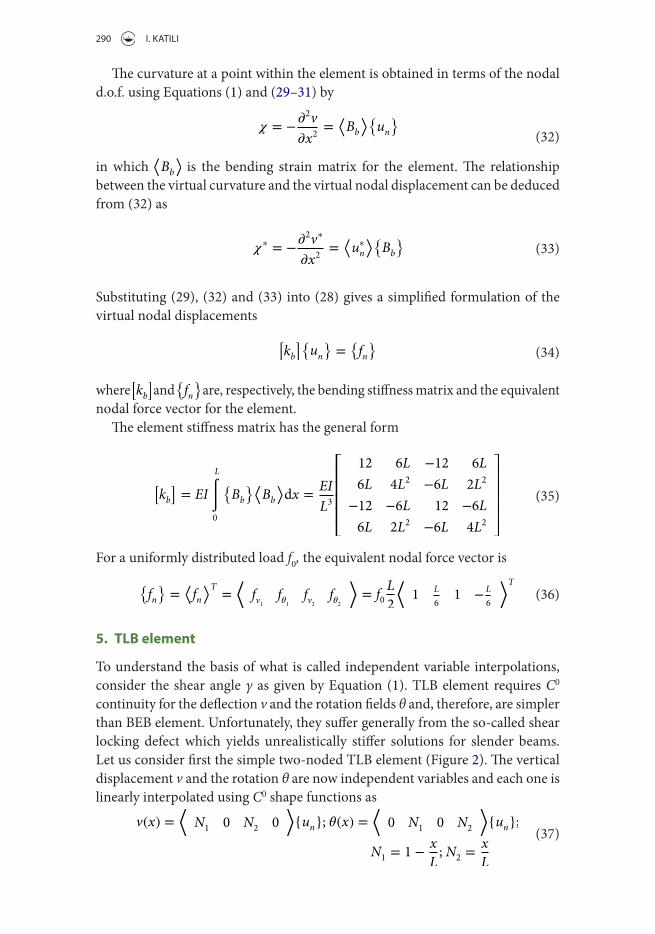
290 I. KATILI
The curvature at a point within the element is obtained in terms of the nodal d.o.f. using Equations (1) and (29–31) by
in which ⟨Bb
⟩ is the bending strain matrix for the element. The relationship
between the virtual curvature and the virtual nodal displacement can be deduced from (32) as
Substituting (29), (32) and (33) into (28) gives a simplified formulation of the virtual nodal displacements
where [kb] and
fn are, respectively, the bending stiffness matrix and the equivalent
nodal force vector for the element.The element stiffness matrix has the general form
For a uniformly distributed load f0, the equivalent nodal force vector is
5. TLB element
To understand the basis of what is called independent variable interpolations, consider the shear angle γ as given by Equation (1). TLB element requires C0 continuity for the deflection v and the rotation fields θ and, therefore, are simpler than BEB element. Unfortunately, they suffer generally from the so-called shear locking defect which yields unrealistically stiffer solutions for slender beams. Let us consider first the simple two-noded TLB element (Figure 2). The vertical displacement v and the rotation θ are now independent variables and each one is linearly interpolated using C0 shape functions as
(32) = −
2v
x2=⟨Bb
⟩un
(33)∗ = −2v∗
x2=⟨u∗
n
⟩Bb
(34)[kb]un
=fn
(35)kb= EI
L
∫0
Bb
Bb
dx =
EI
L3
⎡⎢⎢⎢⎢⎣
12 6L −12 6L
6L 4L2 −6L 2L2
−12 −6L 12 −6L
6L 2L2 −6L 4L2
⎤⎥⎥⎥⎥⎦
(36)fn=⟨fn⟩T
=
⟨fv1 f
1fv2 f
2
⟩= f0
L
2
⟨1 L
61 −
L
6
⟩T
(37)v(x) =
⟨N
10 N
20
⟩un; (x) =
⟨0 N
10 N
2
⟩un;
N1= 1 −
x
L; N
2=
x
L

EUROPEAN JOURNAL OF COMPUTATIONAL MECHANICS 291
where un
is the nodal displacement vector for the element, v1, θ1 and v2, θ2 are
the deflection and the rotation of nodes 1 and 2, respectively, and N1 and N2 are the standard C0 linear shape functions.
The bending strain χ and the transverse shear strain γ are expressed in terms of the nodal d.o.f. using (1) as
For very slender beams γ should vanish. Substituting (38) and (39) into (26), the PVW for an individual element can be written as
After simplifying the virtual displacements
The split of the element stiffness matrix (41) is more convenient as it allows us to identify the bending and shear contributions. The equivalent nodal force vector due to the uniform distributed loading f0:
For all elements with shear effect included, we introduce shear influence factor:
From (41) we obtain the bending stiffness [kb] and the shear stiffness [ks], respectively
The total element stiffness matrix is
(38) = −d
dx=⟨Bb
⟩un
=
⟨0 1
L0 −
1
L
⟩un
(39) =dv
dx− = ⟨Bs⟩un =
−1
L− 1 +
x
L
1
L−
x
L
un.
(40)We =
⟨u∗
n
⟩ ([k]un
−fn)
= 0
(41)
[k]un = fn; [k] = [kb] + [ks]; [kb] = ∫L
0
BbEI⟨Bb
⟩dx;
[ks] = ∫L
0
BskGA⟨Bs
⟩dx
(42)⟨fn⟩= f0 ∫
L
0
⟨N1 0 N2 0
⟩dx =
1
2f0L
⟨1 0 1 0
⟩
(43) =EI
kGA
12
L2
(44)kb=
EI
L3
⎡⎢⎢⎢⎢⎣
0 0 0 0
L2 0 −L2
0 0
sym L2
⎤⎥⎥⎥⎥⎦;ks=
EI
L3
1
⎡⎢⎢⎢⎢⎣
12 6L −12 6L
4L2 −6L 2L2
12 −6L
sym 4L2
⎤⎥⎥⎥⎥⎦

292 I. KATILI
A small value of ϕ indicates that shear strain effects are negligible. The value of ϕ depends on the geometry and the material properties of the transverse cross section. The effect of transverse shear deformation is negligible for a slender beam. Hence, Timoshenko solution should coincide for this case with that of conven-tional Bernoulli–Euler theory. For very slender beams ϕ→0, γ→0 and shear stiffness [ks] should vanish. However, from (44–45), as the beam slenderness increases the numerical solution is progressively stiffer than the exact one. This means that the two-noded TLB element is unable to reproduce the conventional solution for slender beams. For slender beams, if we increase the number of elements, the value of ϕ will increase and the element converge to the exact solution. This phenomenon, known as shear locking, in principle disqualifies TLB element for analysis of slender beams.
6. DSG element
Many procedures to eliminate shear locking in TLB element haves been proposed. One alternative for eliminating shear locking is the so-called ANS. The expression of PVW (26) has to be changed to
The method called DSG proposed by Bletzinger et al. (2000). This method is based on the explicit satisfaction of the kinematic equation for the shear strains at discrete points and effectively eliminates the parasitic shear strains. The essen-tial step is the calculation of DSG at the nodes and their interpolation across the element domain (Figure 2). The total displacement v of the beam is due to defor-mation with respect to bending and shear. The shear related part is determined by integration of (1):
which describes the increase in displacement due to shear between the positions x0 and x. This displacement is identified as shear gap.
The shear gap is evaluated at node i with coordinate xi (x1 = 0 and x2 = L):
(45)k=kb+ks=
EI
L3
1
⎡⎢⎢⎢⎢⎣
12 6L −12 6L
(4 + )L2 −6L (2 − )L2
12 −6L
(4 + )L2
⎤⎥⎥⎥⎥⎦
(46)L∫0
𝜒∗EI𝜒dx +L∫0
𝛾∗kGA𝛾dx = fL∫0
v∗dx + (𝜃∗)|ΓMM + (v∗)|ΓT
T
(47)Δvs(x) =
x
∫x0
dx = v|xx0 −x
∫x0
dx = Δv − Δvb

EUROPEAN JOURNAL OF COMPUTATIONAL MECHANICS 293
where N1 and N2 is defined in (37). We obtain
The distribution of shear gap across the element is now calculated by interpolation from its nodal value with the standard shape function (37),
Finally, the modification shear is obtained by differentiating (50) with respect to x which yields
A popular method proposed by Hughes et al. (1977) is used to reduce the influence of the transverse shear stiffness by computing (39) at point located at the element centre which gives
In fact, the Equations (51) and (52) are identical and so are the resulting stiffness matrices.
Shear stiffness matrix [ks] can be obtained by substituting (52) into (41) which yields
The bending strain (38) and the bending stiffness [kb] (44) are still applicable.The total stiffness matrix for DSG element
(48)Δvsi(x) =
xi
∫0
(x)dx = v|xi0−
xi
∫0
(x)dx = v|xi0−
xi
∫0
(N11 + N22
)dx
(49)Δvs1 = 0 and Δvs2 = v2 − v1 −L
2
(1 + 2
)
(50)Δvs(x) = N1Δvs1 + N2Δvs2 =x
L
(v2 − v1 −
L
2
(1 + 2
))
(51) =dΔvsdx
=⟨Bs
⟩un
=
⟨−
1
L−
1
2
1
L−
1
2
⟩un
(52)−
(x =
1
2L)=⟨Bs
⟩un
=
⟨−
1
L−
1
2
1
L−
1
2
⟩un
(53)ks=
EI
L3
1
⎡⎢⎢⎢⎢⎣
12 6L −12 6L
3L2 −6L 3L2
12 −6L
sym 3L2
⎤⎥⎥⎥⎥⎦; =
EI
kGA
12
L2
(54)k=kb+ks=
EI
L3
1
⎡⎢⎢⎢⎢⎣
12 6L −12 6L
(3 + )L2 −6L (3 − )L2
12 −6L
(3 + )L2
⎤⎥⎥⎥⎥⎦

294 I. KATILI
For very slender beams ϕ→0, γ→0 and shear stiffness [ks] should vanish. However, from (53–54), as the beam slenderness increases the numerical solution is pro-gressively stiffer than the exact one. This means that the two-noded DSG beam element needs more than one element to avoid shear locking and to reproduce the conventional solution for slender beams.
7. DSB element
In this element, rotation θ on node 1 and 2 are approximated using linier inter-polation, while the rotation on element mid-node (node 3) is approximated using quadratic interpolation (Figure 4). This is done in order to get a better model of element behaviour with regard to the rotation effect.
Quadratic increment of rotation is represented by a temporary degree of free-dom, Δθ3. This temporary d.o.f will be later eliminated discretely at the time we formulate the stiffness matrix of DSB element.
The quadratic function is given as follow
where N1 and N2 are as given in Equation (37) and N3 =4x
L
(1 − x
L
).
The shear deformation from (1):
The shear deformation from (16):
Shear influence factor ϕ here has the role to maintain the DSB element consist-ency so as to behave accordingly to the beam theory of Bernoulli–Euler for thin beam analysis (L/h > 20) and behave in accordance with the beam theory of Timoshenko for thick to thin beam (L/h > 4). In the thick beam analysis, shear influence factor ϕ must be taken into account in the stiffness matrix formulation,
(55)(x) = N1 1 + N2 2 + N3 Δ3
(56) =dv
dx−
(57) = −EI
kGA
d2
dx2=
2
3 Δ3 ; =
EI
kGA
12
L2
x1 = 0 x2 = L
31 1 1,f 2
2 2,fvy,
EIx
L1 1vf ,v
2 2vf ,v
Figure 4. DsB element.

EUROPEAN JOURNAL OF COMPUTATIONAL MECHANICS 295
whereas in the thin beam analysis ϕ will approaches zero which also means that the shear deformation is almost zero.
The discrete shear method has been used in references (Katili, 1993a, 1993b, 2006; Katili, Batoz et al., 2015; Katili, Maknun et al., 2015; Maknun et al., 2016) as follows
Substituting (55–57) into (58) yields
Substituting (59) into (55) gives
Therefore, the curvature can be obtained from (1)
The shear deformation can be obtained by substituting Δθ3 (59) into (57):
From (41) we obtain the bending stiffness and the shear stiffness, respectively:
(58)
L
∫0
( −
)dx = 0
(59)Δ3 = −3
2 (1 + )
(v2 − v1L
+1
2
(1 + 2
))
(60)
(x) =⟨ (
−6Lx+6x2
L3(1+)
) (1 − x
L−
3Lx−3x2
L2(1+)
) (6Lx−6x2
L3(1+)
) (x
L−
3Lx−3x2
L2(1+)
) ⟩un
(61) = −d
dx=⟨Bb
⟩un
(62)
where⟨Bb
⟩=
1
(1 + )
⟨ (6L−12x
L3
) (4L−6x+L
L2
)−
(6L−12x
L3
) (2L−6x−L
L2
) ⟩
(63) =2
3 Δ3 =
⟨Bs
⟩un
;⟨Bs
⟩=
(1 + )
⟨−
1
L−
1
2
1
L−
1
2
⟩
(64)
kb=
EI
a L3
⎡⎢⎢⎢⎢⎣
12 6L −12 6L
(3 + a) L2 −6L (3 − a) L2
12 −6L
sym (3 + a) L2
⎤⎥⎥⎥⎥⎦;
ks=
EI
aL3
⎡⎢⎢⎢⎢⎣
12 6L −12 6L
3L2 −6L 3L2
12 −6L
sym 3L2
⎤⎥⎥⎥⎥⎦; a =
1 + )
2

296 I. KATILI
The element stiffness matrix DSB is obtained from the sum of bending and shear stiffness matrices:
To this point we know that in a thin beam ϕ ≅ 0 (ϕ approaches zero), matrix [kb] is equivalent to that of the classic element BEB in Section 3 (Katili, 2006).
Many terms in this stiffness matrix contain the factor ϕ. A convenient feature of this stiffness matrix is that when the shear rigidity is small in comparison to the bending energy, the ϕ→0 and the stiffness coefficients immediately assume the classical BEB element.
Substituting (60) and (63) into (66) and then integrating the result with respect to x we obtain
where
c1, c2, c3 and c4, are obtained from the conditions below:
(65)k=kb+ks=
EI
L3
1
(1 + )
⎡⎢⎢⎢⎢⎣
12 6L −12 6L
(4 + )L2 −6L (2 − )L2
12 −6L
sym (4 + )L2
⎤⎥⎥⎥⎥⎦
(66)dv
dx= +
(67)v(x) = Nv1v1 + N
11 + Nv2
v2 + N22 =
⟨Nv
⟩un
(68)
Nv1
= ∫(−6Lx + 6x2 − L2
L3(1 + )
)dx + c
1;
N1
= ∫(1 −
x
L−
3Lx − 3x2
L2(1 + )−
2(1 + )
)dx + c
3
Nv2
= ∫(6Lx − 6x2 + L2
L3(1 + )
)dx + c
2;
N2
= ∫(x
L−
3Lx − 3x2
L2(1 + )−
2(1 + )
)dx + c
4
Nv1(x = 0) = 1; Nv1
(x = L) = 0; Nv2(x = 0) = 0; Nv2
(x = L) = 1
dN1
dx(x = 0) = 1;
dN1
dx(x = L) = 0;
dN2
dx(x = 0) = 0;
dN2
dx(x = L) = 1
We obtain c1 = 1; c2 = 0; c3 =
2(1 + ); c4 =
2(1 + )

EUROPEAN JOURNAL OF COMPUTATIONAL MECHANICS 297
The equivalent nodal load due to uniform load f0 is obtained from the principle of external virtual work and (67–69) as follows:
Where the equivalent nodal force vector:
8. UI element
This new element with two nodes (Figure 5) called UI element is formulated based on unified and integrated approach (15–26). The slope θ and curvature χ has to be continuous to ensure a smooth deflection field and the continuity of the beam slope across adjacent elements requires that the bending displacement vb, rotation θ, and curvature χ are dependent variables. Therefore, the element has six degrees of freedom: vi, θi and χi at each node i, and continuity C2 Hermite shape functions are required. The vertical bending displacement vb is approximated using a 5th degree polynomial expansion.
Substituting the conditions of each node into (72) gives
(69)And
Nv1= 1 −
3Lx2 − 2x3 + L2x
L3(1 + ); N
1=
2x3 + L2x(2 + ) − Lx2(4 + )
2L2(1 + )
Nv2=
3Lx2 − 2x3 + L2x
L3(1 + ); N
2=
2x3 + Lx2(−2 + ) − L2x
2L2(1 + )
(70)Πext =
L
∫0
f0v(x)dx =⟨un
⟩f0
L
∫0
Nv
dx =
⟨un
⟩fn
(71)fn=⟨fn⟩T
=
⟨fv1 f
1fv2 f
2
⟩= f0
L
2
⟨1 L
61 −
L
6
⟩T
(72)vb = ⟨P⟩an =
1 x x2 x3 x4 x5
an;
an =anT
=
a1
a2
a3
a4
a5
a6
T
x1 = 0 x2 = L1 1 1,f
2
2 2,fvy,
EIx
L1 1vf ,v
2 2vf ,v
1 1,f 2 2,f
Figure 5. ui element.

298 I. KATILI
Back substituting (73) into (72) we get
The curvature at a point within the element is obtained in terms of the nodal d.o.f. using Equations (15) and (74) which gives
The shear deformation at a point within the element is obtained in terms of the nodal d.o.f. using Equations (16) and (74) which gives
The bending and shear stiffness for UI element can be expressed by (41). Thus,
(73)
⎧⎪⎪⎪⎪⎨⎪⎪⎪⎪⎩
vb11=
dvb
dx(x = 0)
1= −
d2vb
dx2(x = 0)
vb22=
dvb
dx(x = L)
2= −
d2vb
dx2(x = L)
⎫⎪⎪⎪⎪⎬⎪⎪⎪⎪⎭
=
⎡⎢⎢⎢⎢⎢⎢⎢⎢⎣
1 0 0 0 0 0
0 1 0 0 0 0
0 0 −2 0 0 0
1 L L2 L3 L4 L5
0 1 2L 3L24L3
5L4
0 0 −2 −6L −12L2 −20L3
⎤⎥⎥⎥⎥⎥⎥⎥⎥⎦
⎧⎪⎪⎪⎪⎨⎪⎪⎪⎪⎩
a1
a2
a3
a4
a5
a6
⎫⎪⎪⎪⎪⎬⎪⎪⎪⎪⎭
or
un
=Pn
an→
an=Pn
−1un
(74)vb = ⟨P⟩an= ⟨P⟩Pn
−1un
=
Nvb
un
(75)
⟨Nvb
⟩=
⟨Nvb1
N1
N1
Nvb2N
2
N2
⟩;
⟨un
⟩=
⟨vb
1
1
1
vb2
2
2
⟩
(76)
Nvb1=
(L − x)3(L2 + 3Lx + 6x2
)
L5;N
1=
(L − x)3x(L + 3x)
L4;N
1= −
(L − x)3x2
2L3
Nvb2 =x3(10L2 − 15Lx + 6x2
)
L5;N
2= −
x3(4L2 − 7Lx + 3x2
)
L4;N
2 = −(L − x)2x3
2L3
(77)
= −d2vb
dx2=⟨Bb
⟩un
;⟨Bb
⟩= −
⟨d2Nvb1
dx2
d2N1
dx2
d2N1
dx2
d2Nvb2
dx2
d2N2
dx2
d2N2
dx2
⟩
(78) = −EI
kGA
d3vb
dx3=⟨Bs
⟩un
;
⟨Bs
⟩= −
L2
12
⟨d3Nvb1
dx3
d3N
1
dx3
d3N
1
dx3
d3Nvb2
dx3
d3N
2
dx3
d3N
2
dx3
⟩
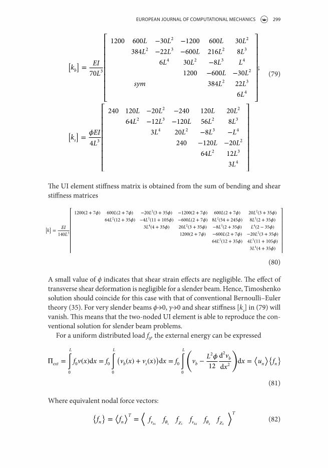
EUROPEAN JOURNAL OF COMPUTATIONAL MECHANICS 299
The UI element stiffness matrix is obtained from the sum of bending and shear stiffness matrices
A small value of ϕ indicates that shear strain effects are negligible. The effect of transverse shear deformation is negligible for a slender beam. Hence, Timoshenko solution should coincide for this case with that of conventional Bernoulli–Euler theory (35). For very slender beams ϕ→0, γ→0 and shear stiffness [ks] in (79) will vanish. This means that the two-noded UI element is able to reproduce the con-ventional solution for slender beam problems.
For a uniform distributed load f0, the external energy can be expressed
Where equivalent nodal force vectors:
(79)
kb=
EI
70L3
⎡⎢⎢⎢⎢⎢⎢⎢⎢⎣
1200 600L −30L2 −1200 600L 30L2
384L2 −22L3 −600L 216L28L3
6L430L2 −8L3 L4
1200 −600L −30L2
sym 384L222L3
6L4
⎤⎥⎥⎥⎥⎥⎥⎥⎥⎦
;
ks=
EI
4L3
⎡⎢⎢⎢⎢⎢⎢⎢⎢⎣
240 120L −20L2 −240 120L 20L2
64L2 −12L3 −120L 56L28L3
3L420L2 −8L3 −L4
240 −120L −20L2
64L212L3
3L4
⎤⎥⎥⎥⎥⎥⎥⎥⎥⎦
(80)
k=
EI
140L3
⎡⎢⎢⎢⎢⎢⎢⎢⎢⎣
1200(2 + 7) 600L(2 + 7) −20L2(3 + 35) −1200(2 + 7) 600L(2 + 7) 20L2(3 + 35)
64L2(12 + 35) −4L3(11 + 105) −600L(2 + 7) 8L2(54 + 245) 8L3(2 + 35)
3L4(4 + 35) 20L2(3 + 35) −8L3(2 + 35) L4(2 − 35)
1200(2 + 7) −600L(2 + 7) −20L2(3 + 35)
64L2(12 + 35) 4L3(11 + 105)
3L4(4 + 35)
⎤⎥⎥⎥⎥⎥⎥⎥⎥⎦
(81)
Πext =
L
∫0
f0v(x)dx = f0
L
∫0
(vb(x) + vs(x)
)dx = f0
L
∫0
(vb −
L2
12
d2vb
dx2
)dx =
⟨un
⟩fn
(82)fn=⟨fn⟩T
=
⟨fvb1 f
1f1
fvb2 f2
f2
⟩T

300 I. KATILI
From (18) if vertical displacements at the nodes are zero, they can be formulated as follows:
9. Numerical application
In this section examples with different boundary conditions are presented to illustrate the performance of several elements in static analysis. Those considered include the BEB, TLB, DSG, DSB and UI elements.
9.1. Beam with uniform load and different boundary conditions
9.1.1. Cantilever beamA cantilever beam fixed at node 1 and free at node 2 is subject to a uniform load f0 (Figure 6). The total displacement v and rotation θ at node 2 and displacement functions along the beam resulting from calculation using different elements are shown in Table 1.
(83)⟨fn⟩= f0L
⟨1
2
L(6+5)
60−
L2
120
1
2−
L(6+5)
60−
L2
120
⟩
(84)At node 1: v1 = vb1 +L2
121 = 0 → vb1 = −
L2
121
(85)At node 2: v2 = vb2 +L2
122 = 0 → vb2 = −
L2
122
Figure 6. Cantilever beam.
Table 1. results of cantilever beam using one element.
Element Displacement functions v2 θ2
BEB v(x) =f0L
24EIx(5Lx − 2x
2)
f0L4
24EI(3)
f0L3
6EI
tlBv(x) =
f0L3
24EI
x(4+)
(1+)
f0L4
24EI
(4+)
(1+)
f0L3
4EI
(1+)
DsGv(x) =
foL3x(3+)
24EI
f0L4
24EI(3 + )
f0L3
4EI
DsB v(x) =f0L
24EIx(5Lx − 2x
2+ L
2)
f0L4
24EI(3 + )
f0L3
6EI
ui v(x) =f0
24EIx(x3− 4Lx
2+ 6L
2x + L2(2L − x)
)f0L4
24EI(3 + )
f0L3
6EI
EXaCt v(x) =f0
24EIx(x3− 4Lx
2+ 6L
2x + L2(2L − x)
)f0L4
24EI(3 + )
f0L3
6EI

EUROPEAN JOURNAL OF COMPUTATIONAL MECHANICS 301
In thin beam ϕ ≅ 0 (ϕ approaches zero), TLB element suffers from shear locking, as the number of element increases, the value of ϕ will increase and the results will slowly converge to the exact solution. With one element, DSG element can only give an exact value of v2 and DSB element cannot give an exact displacement functions as can be seen in Table 1.
9.1.2. Simple supported beam
Results from UI element (Figure 6):
⎧⎪⎪⎪⎪⎨⎪⎪⎪⎪⎩
vb11
1
vb22
2
⎫⎪⎪⎪⎪⎬⎪⎪⎪⎪⎭
=f0L
2
24EI
⎧⎪⎪⎪⎪⎨⎪⎪⎪⎪⎩
L2
0
−12
L2(3 + )
4L
0
⎫⎪⎪⎪⎪⎬⎪⎪⎪⎪⎭
Results from UI element (Figure 7):
⎧⎪⎪⎪⎪⎨⎪⎪⎪⎪⎩
vb11
1
vb22
2
⎫⎪⎪⎪⎪⎬⎪⎪⎪⎪⎭
=f0L
3
24EI
⎧⎪⎪⎪⎪⎨⎪⎪⎪⎪⎩
0
1
0
0
−1
0
⎫⎪⎪⎪⎪⎬⎪⎪⎪⎪⎭
Table 2. results of simple supported beam using one element.
Element Displacement functions θ1 θ2
BEBv(x) =
f0L2
24EIx(L − x)
f0L3
24EI−
f0L3
24EI
tlB v(x) = 0 0 0
DsG v(x) = 0 0 0
DsBv(x) =
f0L2
24EIx(L − x)
f0L3
24EI−
f0L3
24EI
ui v(x) =f0
24EIx(x3− 2Lx
2+ L
3+ L
2(L − x))
f0L3
24EI−
f0L3
24EI
EXaCt v(x) =f0
24EIx(x3− 2Lx
2+ L
3+ L
2(L − x))
f0L3
24EI−
f0L3
24EI
Figure 7. simple supported beam.

302 I. KATILI
The rotation θ at node 1 and at node 2 and displacement functions along the beam resulting from calculation using different elements are shown in Table 2. With one element, TLB and DSG elements cannot give nodal values and DSB element cannot give an exact displacement function (Figure 7, Table 2).
9.1.3. Fixed-simple supported beam
The rotation θ at node 2 and displacement functions along the beam resulting from calculation using different elements are shown in Table 3. With only one element, TLB and DSG elements cannot give nodal values and DSB element cannot give an exact displacement function (Figure 8, Table 3).
Results from UI element (Figure 8):
⎧⎪⎪⎪⎪⎨⎪⎪⎪⎪⎩
vb11
1
vb22
2
⎫⎪⎪⎪⎪⎬⎪⎪⎪⎪⎭
=f0L
2
24EI(4 + )
⎧⎪⎪⎪⎪⎨⎪⎪⎪⎪⎩
L2
0
−12
0
−2L(1 + )
0
⎫⎪⎪⎪⎪⎬⎪⎪⎪⎪⎭
Table 3. results of fixed-simple supported beam with one element.
Element Displacement functions θ2
BEB v(x) =f0L
48EIx2(L − x) −
f0L3
48EI
tlB v(x) = 0 0
DsG v(x) = 0 0
DsB v(x) =f0L
24EI(4+)x(L − x)(2x + L) −
f0L3
12EI
(1+)
(4+)
ui v(x) =f0
24EI(4+)x(L − x)
(Lx(6 + ) − x
2(4 + ) + L
2(5 + ))
−f0L3
12EI
(1+)
(4+)
EXaCt v(x) =f0
24EI(4+)x(L − x)
(Lx(6 + ) − x
2(4 + ) + L
2(5 + ))
−f0L3
12EI
(1+)
(4+)
Figure 8. fixed-simple supported beam.

EUROPEAN JOURNAL OF COMPUTATIONAL MECHANICS 303
9.1.4. Simple-fixed roll supported beam
The rotation θ at node 1 and displacement at node 2 and displacement functions along the beam resulting from calculation using different elements are shown in Table 4. In thin beam ϕ ≅ 0 (ϕ approaches zero), TLB element suffers from shear locking, by increasing the number of element, the value of ϕ will increase and the results will converge to the exact solution. Compared to the exact solution, TLB and DSG element give the different values of θ1 and v2. DSB element cannot give an exact displacement function (Figure 9, Table 4).
Results from UI element (Figure 9):
⎧⎪⎪⎪⎪⎨⎪⎪⎪⎪⎩
vb11
1
vb22
2
⎫⎪⎪⎪⎪⎬⎪⎪⎪⎪⎭
=f0L
2
24EI
⎧⎪⎪⎪⎪⎨⎪⎪⎪⎪⎩
0
8L
0
5L2
0
12
⎫⎪⎪⎪⎪⎬⎪⎪⎪⎪⎭
Table 4. results of simple-fixed roll supported beam with one element.
Element Displacement functions θ1 v2
BEB v(x) =f0L
24EIx(8L
2− Lx − 2x
2)
f0L3
3EI
f0L4
24EI(5)
tlBv(x) = −
f0L3
24EIx
(4+)
(1+)
f0L3
4EI
(1+)
f0L4
24EI
(4+)
(1+)
DsGv(x) =
f0L3
24EIx(3 + )
f0L3
4EI
f0L4
24EI(3 + )
DsB v(x) =f0L
24EIx(8L
2− Lx − 2x
2+ L
2)
f0L3
3EI
f0L4
24EI(5 + )
ui v(x) =f0
24EIx(x3− 4Lx
2+ 8L
3+ L
2(2L − x))
f0L3
3EI
f0L4
24EI(5 + )
EXaCt v(x) =f0
24EIx(x3− 4Lx
2+ 8L
3+ L
2(2L − x))
f0L3
3EI
f0L4
24EI(5 + )
Figure 9. simple-fixed roll supported beam.

304 I. KATILI
9.1.5. Fixed-fixed roll supported beam
Displacement at node 2 and displacement functions along the beam resulting from calculation using different elements are shown in Table 5. In thin beam ϕ ≅ 0 (ϕ approaches zero), TLB and DSG elements suffer from shear locking, however, by increasing the number of element, the value of ϕ will increase and the results will converge to the exact solution. DSB element cannot give an exact displacement functions (Figure 10, Table 5).
Results from UI element (Figure 10):
⎧⎪⎪⎪⎪⎨⎪⎪⎪⎪⎩
vb11
1
vb22
2
⎫⎪⎪⎪⎪⎬⎪⎪⎪⎪⎭
=f0L
2
72EI
⎧⎪⎪⎪⎪⎨⎪⎪⎪⎪⎩
2L2
0
−24
L2(3 + 2)
0
12
⎫⎪⎪⎪⎪⎬⎪⎪⎪⎪⎭
Figure 10. fixed-fixed roll supported beam.
Table 5. results of fixed-fixed roll supported beam with one element.
Element Displacement functions v2
BEB v(x) =f0L
24EIx(3Lx − 2x
2)
f0L4
24EI
tlBv(x) =
f0L3
24EIx
f0L4
24EI
DsGv(x) =
f0L3
24EIx
f0L4
24EI
DsB v(x) = −f0L
24EIx(3Lx − 2x
2+ L
2)
f0L4
24EI(1 + )
ui v(x) =f0
24EIx(x3− 4Lx
2+ 4L
2x + L
2(2L − x))
f0L4
24EI(1 + )
EXaCt v(x) =f0
24EIx(x3− 4Lx
2+ 4L
2x + L
2(2L − x))
f0L4
24EI(1 + )

EUROPEAN JOURNAL OF COMPUTATIONAL MECHANICS 305
9.1.6. Fixed-fixed supported beam
With one element, only UI element can give an exact displacement function (Figure 11, Table 6).
9.2. Convergence studies
For the next two problems let us consider a uniform loaded beam with length thickness ratio L/h = 4 in two different boundary conditions, i.e. simple-fixed roll and fixed-fixed roll (Figure 12). The vertical displacement (v2) of slider support on the right end of the beam is observed for each problem. For the computations, a rectangular cross-section and the following geometrical and material parame-ters: length 1 m, width 0.1 m, thickness 0.25 m, Young’s modulus E =107 kN/m2, Poisson’s ratio 0.2 and a shear correction factor of k = 5/6 are used.
In the case of thick beam it can be seen that comparative studies using 1, 2, 4, 6, 8, 10 numbers of element (NELT) or using number of degree of freedom (NDOF), the BEB gives the Bernoulli–Euler solution for thin beam (shear effect excluded),
Results from UI element (Figure 11):
⎧⎪⎪⎪⎪⎨⎪⎪⎪⎪⎩
vb11
1
vb22
2
⎫⎪⎪⎪⎪⎬⎪⎪⎪⎪⎭
=f0L
2
144EI
⎧⎪⎪⎪⎪⎨⎪⎪⎪⎪⎩
L2
0
−12
L2
0
−12
⎫⎪⎪⎪⎪⎬⎪⎪⎪⎪⎭
Figure 11. fixed-fixed supported beam.
Table 6. results of fixed-fixed supported beam with one element.
Element Displacement functionsBEB v(x) = 0
tlB v(x) = 0
DsG v(x) = 0
DsB v(x) = 0
ui v(x) =f0
24EIx(x3− 2Lx
2+ L
2x + L
2(L − x))
EXaCt v(x) =f0
24EIx(x3− 2Lx
2+ L
2x + L
2(L − x))

306 I. KATILI
(a)
(b)
f 0
12
f 0
12
f 0
12
f 0
12
Figu
re 1
2. C
onve
rgen
ce st
udie
s for
a th
ick
beam
(L/h =
4).
(a) s
impl
e-fix
ed ro
ll. (b
) fix
ed-fi
xed
roll.

EUROPEAN JOURNAL OF COMPUTATIONAL MECHANICS 307
the TLB and DSG need more than one element to converge to the Timoshenko exact solution, while DSB and UI elements only need one element to give the exact solution. The difference between DSB and UI element is that DSB gives the exact solution only on nodes, while UI element gives the exact solution at any point of the beam.
10. Conclusion
Based on the results obtained from the numerical examination, we can conclude that:
(1) BEB element is only valid for thin beam as its formulation neglects the effect of shear deformation.
(2) TLB element is disqualified for analysis of slender beams as it suffers from severe shear locking. For slender beams, it only shows convergence to the exact solution if a large number of elements is used.
(3) With only one element, DSG element still suffers from shear locking and thus cannot give an exact value. Using more than one element this shear locking will vanish and DSG will converge to the exact solution.
(4) DSB element give an exact d.o.f. values.(5) Although UI element uses more d.o.f., it is more efficient than the stand-
ard beam elements. All presented tests indicate that UI element is able to give exact d.o.f. values and exact displacement function even with only one element.
Acknowledgments
The financial support from the Indonesian Ministry of Research, Technology and Higher Education (KEMENRISTEKDIKTI) is gratefully acknowledged.
Disclosure statement
No potential conflict of interest was reported by the author.
Funding
This work was supported by Indonesian Ministry of Research, Technology and Higher Education [KEMENRISTEKDIKTI].
References
Bathe, K. J., & Dvorkin, E. N. (1985). A four-node plate bending element based on Mindlin-Reissner plate theory and a mixed interpolation. International Journal for Numerical Methods in Engineering, 21, 367–383.

308 I. KATILI
Bletzinger, K.-U., Bischoff, M., & Ramm, E. (2000). A unified approach for shear-locking-free triangular and rectangular shell finite elements. Computers and Structures, 75, 321–334.
Falsone, G., & Settineri, D. (2011). An Bernoulli-Euler-like finite element method for Timoshenko beams. Mechanics Research Communications, 38, 12–16.
Hughes, T. J. R., Taylor, R. L., & Kanoknukulchai, W. (1977). A simple and efficient for plate bending. International Journal for Numerical Methods in Engineering, 11, 1529–1543.
Hughes, T. J. R., & Tezduyar, T. E. (1981). Finite element based upon Mindlin plate theory with particular reference to the four-node bilinear isoparametric element. Journal of Applied Mechanics, 48, 587–596.
Kapur, K. (1966). Vibrations of a Timoshenko beam using finite-element approach. The Journal of the Acoustical Society of America, 40, 1058–1063.
Katili, I. (1993a). A new discrete Kirchhoff-Mindlin element based on Mindlin-Reissner plate theory and assumed shear strain fields- part I: An extended DKT element for thick-plate bending analysis. International Journal for Numerical Methods in Engineering, 36, 1859–1883.
Katili, I. (1993b). A new discrete Kirchhoff-Mindlin element based on Mindlin-Reissner plate theory and assumed shear strain fields- part II: An extended DKQ element for thick plate bending analysis. International Journal for Numerical Methods in Engineering, 36, 1885–1908.
Katili I. (2006). Metode Elemen Hingga untuk Skeletal. Jakarta: Rajawali Press.Katili, I., Batoz, J. L., Maknun, I. J., Hamdouni, A., & Millet, O. (2015). The development of
DKMQ plate bending element for thick to thin shell analysis based on Naghdi/Reissner/Mindlin shell theory. Finite Elements in Analysis and Design, 100, 12–27.
Katili, I., Maknun, I. J., Hamdouni, A., & Millet, O. (2015). Application of DKMQ element for composite plate bending structures. Composite Structures Journal, 132, 166–174.
Kiendl, J., Auricchio, F., Hughes, T. J. R., & Reali, A. (2015). Single-variable formulations and isogeometric discretizations for shear deformable beams. Computer Methods in Applied Mechanic and Engineering, 284, 988–1004.
Li, X.-F. (2008). A unified approach for analyzing static and dynamic behavior of functionally graded Timoshenko and Bernoulli-Euler beam. Journal of Sound Vibration, 318, 1210–1229.
Maknun, I. J., Katili, I., Millet, O., & Hamdouni, A. (2016). Application of DKMQ element for twist of thin-walled beams: Comparison with Vlasov theory. International Journal for Computational Methods in Engineering Science and Mechanics, 17, 391–400.
Timoshenko, S. (1921). On the correction for shear of differential equation for transverse vibrations of prismatic bars. Philosophical Magazine, 41, 744–746.
Timoshenko, S. (1922). On the transverse vibrations of bars of uniform cross section. Philosophical Magazine, 43, 125–131.