unification source-tracking with … source-tracking with application to diagnosis of type inference...
TRANSCRIPT
UNIFICATION SOURCE-TRACKING WITH
APPLICATION TO DIAGNOSIS OF TYPE INFERENCE
Venkatesh Choppella
Computer Science Department
Indiana University
Submitted to the faculty of the Graduate School
in partial fulfillment of the requirements
for the degree
Doctor of Philosophy
in the Department of Computer Science
Indiana University
August 2002

Accepted by the Graduate Faculty, Indiana University, in partial fulfillment
of the requirements of the degree of Doctor of Philosophy.
DoctoralCommittee
Christopher T. Haynes, Ph.D.(Principal Advisor)
Daniel P. Friedman, Ph.D.
Steven D. Johnson, Ph.D.
Paul W. Purdom, Ph.D.
July 10th, 2002 Lawrence S. Moss, Ph.D.
ii
Copyright c 2002
Venkatesh Choppella
Computer Science Department
Indiana University
ALL RIGHTS RESERVED
iii

To my mother Srimati Sundari, and father Sri Choppella Venkata Ramachandra Murti, and
to the memory of my grandmother Srimati Parupalli Sitaratnam
iv
Acknowledgements
I owe a great debt of gratitude to Chris Haynes, my thesis advisor. This thesis would not
have been accomplished without his enthusiastic support and encouragement. His unfailing
confidence in my abilities steered me through the many dark corners and dead ends that are
an inevitable part of research.
I was fortunate to have a strong and supportive research committee. I owe a special
debt of gratitude to Larry Moss, who taught me co-induction and offered crucial advice on
many technical issues. The flat system formalism used in this thesis is inspired by his work.
Steve Johnson introduced me to theorem proving and gave me the opportunity to hang out
in his lab and collaborate with his students. Dan Friedman taught me what to value in
programming. Paul Purdom helped me understand several points about unification and
rewrite systems. Each of them read my thesis with critical attention and offered valuable
advice. To all of them, my deep-felt gratitude.
I wish to thank Gregor Kiczales and his Aspect-Oriented Programming group for the
v

very enjoyable time I spent at the Xerox Palo Alto Research Center. Aspects provided a
fresh perspective to my thinking on the problem of debugging. At a time when people
were being lured into Silicon Valley startups, Gregor encouraged me to instead head back
to school and attend to my unfinished dissertation. I thank him for his sound advice.
I appreciate and thank the administrative and systems staff of the computer science
department at IU for going out of their way to help me on many occasions. They clearly
stand out as among the best anywhere.
My stay in the beautiful town of Bloomington was made all the more memorable by the
large number of wonderful friends I made during the years. I want to specially thank all of
them for their friendship.
My greatest debt of gratitude goes to my family. I thank my parents for their affection
and support and dedicate this thesis to them. Finally, I want to thank my dear wife Shailaja.
Her love and many sacrifices made this thesis possible.
vi
Abstract
Prior diagnoses in unification-based type reconstruction systems have either missed
information that is relevant, presented irrelevant details, or both.
We use a framework based on the Unification Logics of Le Chenadec to define, de-
rive and simplify proof-based source-tracking for term unification. The objects of source-
tracking are proofs in this deduction system, and correspond to path expressions over a
unification graph whose labels form a semi-Dyck language of balanced parentheses. Sim-
plification of source-tracking information is implemented as proof normalization in the
rewrite system for free groups. Subject-reduction properties guarantee that normalization
preserves the semantics of deductions. The presentation of the logic facilitates proof con-
struction by a simple extension to standard unification algorithms.
We apply unification source-tracking to type inference in the Curry-Hindley type sys-
tem. Programs are represented as systems of syntax equations. Program slices correspond
vii
to weakenings of syntax and type equations. A constraint generation function maps weak-
enings of type equations to weakenings of syntax equations. Source-tracking information
is defined in terms of the inverse of this generating function.
Unification is central to many applications of symbolic computation and artificial in-
telligence, including computer algebra, automated theorem proving, expert systems, and
programming language type systems. Source-tracking is a debugging technique based on
tracing the execution of a program to identify those subparts that contribute to the result of
the execution.
viii

Contents
Acknowledgements v
Abstract vii
1 Introduction 1
1.1 Diagnosis of computer errors . . . . . . . . . . . . . . . . . . . . . . . . . 1
1.2 Term unification and type inference . . . . . . . . . . . . . . . . . . . . . 2
1.3 Inadequate type error diagnosis in ML: two simple programs . . . . . . . . 6
1.3.1 Diagnostic analysis of the program in Experiment 1 . . . . . . . . . 11
1.4 Contributions of the thesis . . . . . . . . . . . . . . . . . . . . . . . . . . 21
1.5 Organization of the thesis . . . . . . . . . . . . . . . . . . . . . . . . . . . 23
2 Related Research 25
ix
2.1 Type Error Diagnosis: Previous attempts . . . . . . . . . . . . . . . . . . . 25
2.1.1 Wand’s algorithm . . . . . . . . . . . . . . . . . . . . . . . . . . . 25
2.1.2 Attribute Grammars and flow information . . . . . . . . . . . . . . 28
2.1.3 Partial Type Inference . . . . . . . . . . . . . . . . . . . . . . . . 29
2.1.4 Tracing Techniques . . . . . . . . . . . . . . . . . . . . . . . . . . 31
2.1.5 Explanation and Visualization-based systems . . . . . . . . . . . . 31
2.1.6 Program Slicing . . . . . . . . . . . . . . . . . . . . . . . . . . . 33
2.2 Logic Programming and unification-based systems . . . . . . . . . . . . . 34
2.3 Unification Logics of Le Chenadec . . . . . . . . . . . . . . . . . . . . . . 36
2.4 Diagnosis in Artificial Intelligence . . . . . . . . . . . . . . . . . . . . . . 38
3 A review of term unification 39
3.1 Basic Definitions . . . . . . . . . . . . . . . . . . . . . . . . . . . . . . . 42
3.1.1 Relations . . . . . . . . . . . . . . . . . . . . . . . . . . . . . . . 42
3.1.2 Directed Graphs . . . . . . . . . . . . . . . . . . . . . . . . . . . 43
3.1.3 Alphabet, sentences, signature . . . . . . . . . . . . . . . . . . . . 44
3.1.4 Labeled directed graphs, �-graphs . . . . . . . . . . . . . . . . . . 45
3.2 Rational Terms . . . . . . . . . . . . . . . . . . . . . . . . . . . . . . . . 47
x
3.2.1 Flat Systems . . . . . . . . . . . . . . . . . . . . . . . . . . . . . 50
3.2.2 Term Graphs . . . . . . . . . . . . . . . . . . . . . . . . . . . . . 52
3.2.3 Term-bisimulation . . . . . . . . . . . . . . . . . . . . . . . . . . 54
3.3 Substitutions . . . . . . . . . . . . . . . . . . . . . . . . . . . . . . . . . 56
3.4 Unification . . . . . . . . . . . . . . . . . . . . . . . . . . . . . . . . . . 58
3.4.1 Unification graphs . . . . . . . . . . . . . . . . . . . . . . . . . . 60
3.4.2 Unifiability . . . . . . . . . . . . . . . . . . . . . . . . . . . . . . 62
3.4.3 Unification closure . . . . . . . . . . . . . . . . . . . . . . . . . . 67
3.4.4 Construction of Most General Unifiers . . . . . . . . . . . . . . . . 71
3.5 The unification algorithm . . . . . . . . . . . . . . . . . . . . . . . . . . . 76
3.6 Summary . . . . . . . . . . . . . . . . . . . . . . . . . . . . . . . . . . . 82
4 Path expression logics for unifiability 84
4.1 Preliminaries . . . . . . . . . . . . . . . . . . . . . . . . . . . . . . . . . 87
4.1.1 �-Algebras . . . . . . . . . . . . . . . . . . . . . . . . . . . . . . 87
4.1.2 Semi-Dyck and Dyck languages . . . . . . . . . . . . . . . . . . . 89
4.1.3 �-graph representation of unification graphs . . . . . . . . . . . . 95
4.2 Path Logics . . . . . . . . . . . . . . . . . . . . . . . . . . . . . . . . . . 98
xi
4.2.1 Paths over labeled directed graphs . . . . . . . . . . . . . . . . . . 98
4.2.2 Bidirectional Paths . . . . . . . . . . . . . . . . . . . . . . . . . . 100
4.2.3 Computation of shortest unification paths . . . . . . . . . . . . . . 108
4.3 Logic of unification paths . . . . . . . . . . . . . . . . . . . . . . . . . . . 109
4.4 Logic of Unification Path Expressions . . . . . . . . . . . . . . . . . . . . 112
4.4.1 Normalization . . . . . . . . . . . . . . . . . . . . . . . . . . . . 115
4.5 Unification Algorithm with source-tracking . . . . . . . . . . . . . . . . . 117
4.6 Summary . . . . . . . . . . . . . . . . . . . . . . . . . . . . . . . . . . . 122
5 Error reconstruction in Curry-Hindley Type Inference 123
5.1 Type Systems . . . . . . . . . . . . . . . . . . . . . . . . . . . . . . . . . 126
5.2 Preliminaries: Partial Orders . . . . . . . . . . . . . . . . . . . . . . . . . 129
5.2.1 �-Graph simulations . . . . . . . . . . . . . . . . . . . . . . . . . 131
5.3 The CH type system: syntax and type rules . . . . . . . . . . . . . . . . . 132
5.3.1 Abstract Syntax graphs representations of closed �-expressions . . 133
5.3.2 CH Type Rules . . . . . . . . . . . . . . . . . . . . . . . . . . . . 134
5.4 Subset-based generating function for CH . . . . . . . . . . . . . . . . . . . 137
5.4.1 Untypability of subsets of syntax equations . . . . . . . . . . . . . 141
xii

5.5 Weakenings of type equations . . . . . . . . . . . . . . . . . . . . . . . . 144
5.6 Weakening-based generating function for CH . . . . . . . . . . . . . . . . 148
5.7 Non-unifiability and untypability of weakenings . . . . . . . . . . . . . . . 150
5.7.1 Untypability of weak syntax equations . . . . . . . . . . . . . . . . 151
5.8 Properties of source functions . . . . . . . . . . . . . . . . . . . . . . . . 157
5.8.1 Locality . . . . . . . . . . . . . . . . . . . . . . . . . . . . . . . . 157
5.8.2 Linearity . . . . . . . . . . . . . . . . . . . . . . . . . . . . . . . 158
5.9 Summary . . . . . . . . . . . . . . . . . . . . . . . . . . . . . . . . . . . 159
6 Conclusions and Future Work 160
6.1 Conclusions . . . . . . . . . . . . . . . . . . . . . . . . . . . . . . . . . . 160
6.2 Immediate Extensions . . . . . . . . . . . . . . . . . . . . . . . . . . . . . 162
6.2.1 Damas-Milner Type Inference . . . . . . . . . . . . . . . . . . . . 162
6.2.2 Equational and Semi-unification . . . . . . . . . . . . . . . . . . . 165
6.3 Other Applications . . . . . . . . . . . . . . . . . . . . . . . . . . . . . . 167
6.3.1 Source-tracking of Prolog programs . . . . . . . . . . . . . . . . . 167
6.3.2 Soft-typing . . . . . . . . . . . . . . . . . . . . . . . . . . . . . . 167
6.4 Automated debugging . . . . . . . . . . . . . . . . . . . . . . . . . . . . . 168
xiii

List of Figures
1.1 Experiment 1: Example program showing redundant type error information
generated by the Standard ML of New Jersey compiler. Text in boldface
typewriter font refers to user input. Text in regular typewriter font refers to
the output of the compiler. Text following // denotes a comment. . . . . . 8
1.2 Experiment 2: Example program showing insufficient type error informa-
tion generated by the Standard ML of New Jersey compiler. Text enclosed
in angle brackets of the error message denotes program parts deemed un-
necessary for the reconstruction of the error by the compiler. . . . . . . . . 9
1.3 Parse tree of example program e of Experiment 1 . . . . . . . . . . . . . . 12
1.4 Syntax equations describing the parse tree of the example program . . . . . 12
1.5 Type Rules used for computing the type of the example program . . . . . . 13
1.6 Syntactic constraints and type constraints generated from them for the ex-
ample program. . . . . . . . . . . . . . . . . . . . . . . . . . . . . . . . . 14
xiv

1.7 Unification closure rules for type terms formed using a single binary func-
tor !. . . . . . . . . . . . . . . . . . . . . . . . . . . . . . . . . . . . . . 15
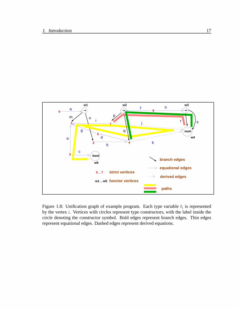
1.8 Unification graph of example program. Each type variable ti is represented
by the vertex i. Vertices with circles represent type constructors, with the
label inside the circle denoting the constructor symbol. Bold edges repre-
sent branch edges. Thin edges represent equational edges. Dashed edges
represent derived equations. . . . . . . . . . . . . . . . . . . . . . . . . . 17
1.9 Graphical representation of syntax equations S1 and S2 . . . . . . . . . . . 21
3.1 Term graph for flat system in Example 3.2.3. The vertex t is isolated. . . . 53
3.2 Unification graph G = hT;Ei for Example 3.4.7. G is the term graph T
augmented with elements of E, which are represented as undirected edges
in G. . . . . . . . . . . . . . . . . . . . . . . . . . . . . . . . . . . . . . 61
3.3 The Unification closure �G of a graph G = hhW;X; bi; Ei. . . . . . . . . 67
3.4 Quotient graph G=� of the graph G in Figure 3.2 . . . . . . . . . . . . . . 69
3.5 Quotient graph G=R of the graph G of Figure 3.2, where R is the equiva-
lence induced by the unifier �� on G computed in Example 3.4.9. . . . . . 71
3.6 Unification algorithm: procedure unify . . . . . . . . . . . . . . . . . . . 77
3.7 Unification algorithm: procedures union and find . . . . . . . . . . . . . . 77
xv
3.8 Unification algorithm: procedure occurs? . . . . . . . . . . . . . . . . . . 78
4.1 Unification graph G of Example 3.4.7 represented as a directed, labeled
graph . . . . . . . . . . . . . . . . . . . . . . . . . . . . . . . . . . . . . 97
4.2 The logic �(G) of paths over G where G is the labeled directed graph
h�V ;�D; V; L;Di . . . . . . . . . . . . . . . . . . . . . . . . . . . . . . . 99
4.3 The logic �2(G) of bidirectional paths over G where G is the labeled di-
rected graph h�V ;�D; V; L;Di . . . . . . . . . . . . . . . . . . . . . . . . 101
4.4 The logic �U(G) of unification paths over G where G is the labeled di-
rected graph G = h�V ;�D; V; L;Di . . . . . . . . . . . . . . . . . . . . . 110
4.5 The logic PU(G) of unification path expressions over a labeled directed
graph G = h�V ;�D; V; L;Di . . . . . . . . . . . . . . . . . . . . . . . . . 113
4.6 Equational rewrite system R=A for free groups, where A consists of the
Equational rule of Associativity and R consists of the remaining rules (Pe-
terson and Stickel, 1981). . . . . . . . . . . . . . . . . . . . . . . . . . . . 115
4.7 Unification algorithm with source-tracking: procedure unify . . . . . . . . 118
4.8 Unification algorithm with source-tracking: procedures union and find . . . 118
4.9 Unification algorithm with source-tracking: procedure occurs? . . . . . . . 119
5.1 ASG for expression in Example 5.3.18 . . . . . . . . . . . . . . . . . . . . 135
xvi
5.2 The CH type inference system . . . . . . . . . . . . . . . . . . . . . . . . 138
5.3 Schemas for the generating function gene mapping equations in be to type
equations in the canonical system Ee of type equations of e in the Curry-
Hindley type system , where Te = hWe; Xe; bei is the ASG of the closed
�-expression e. . . . . . . . . . . . . . . . . . . . . . . . . . . . . . . . . 139
5.4 Unification graph with oriented and labeled edges representing type equa-
tions generated for the expression of Example 5.3.18 . . . . . . . . . . . . 140
5.5 (a) the unification graph of the set of type equations E1 of Example 5.4.20
and (b) syntax equations B1 generating E1. . . . . . . . . . . . . . . . . . 143
5.6 (a) the unification graph of the set of type equations E2 of Example 5.4.20,
and (b) the ASG of the syntax equations B2 generating E2. . . . . . . . . . 145
5.7 Generating function wgene that maps equations in be# to equations in Ee#
in the CH type system , where Te = hWe; Xe; bei is the ASG of e, and Ee
is the canonical set of type equations for e. . . . . . . . . . . . . . . . . . . 149
5.8 (a) The unification graph of the cycle C1 defined in Example 5.7.22, and
(b) the set of weakenings S1 generating the cycle C1 in Example 5.7.22 (the
vertex labeled @ is anonymous). . . . . . . . . . . . . . . . . . . . . . . . 155
xvii
5.9 (a): The cycle C2 defined in Example 5.7.22; (b): Graph representing the
set S2 of weakenings generating the cycle C2 in Example 5.7.22 (one of the
vertices labeled @ is anonymous). . . . . . . . . . . . . . . . . . . . . . . 156
xviii

1
Introduction
1.1 Diagnosis of computer errors
When programs encounter an error, they frequently fail to answer the following ques-
tions in a satisfactory manner:
1. Reporting the symptom of the error: What is the error?
2. Diagnosis, or source-tracking of the error: What caused the error?
3. Correction of the error: How can the error be removed or fixed?
Even if the reporting of the symptom is adequate, programs are poor in communicating the
diagnosis of the error. On the occasions that a diagnosis is offered, it is either too terse,
as seen in operating system error messages (the infamous “bus error” in Unix), or over-
whelming in its prolixity, as seen in some parser error messages of compilers. As a result,
1
1. Introduction 2
a program’s error messages can sometimes be confusing and hard to understand. Finally,
repair of the program is left to the writer of the program. Without adequate diagnosis of the
error, it is hard to repair the program, especially in the absence of proper debugging tools.
1.2 Term unification and type inference
This thesis presents a framework for the formulation, derivation and simplification of
diagnostic information for errors occurring in implementation of two well-known problems
in programming systems: term unification and type inference.
The problem of term unification, first studied by Herbrand [45] in the 1930’s, consists of
automatically solving equations over terms. Terms are built from variables and constructor
symbols. For example, if x, y, u and v denote variables, and f a constructor symbol, then
unifying the terms f(x; y) and f(u; v) means solving the term equation f(x; y) = f(u; v). A
system of equations is unifiable if it has a solution. The example term equation is unifiable
because it has the solution x 7! u; y 7! v. The rules of unification used for solving term
equations consist of the rules of equality, substitution, and equating subterms. Term unifica-
tion has applications in many areas, including automated deduction, artificial intelligence,
and programming languages.
In term unification, errors correspond to the situation when a set of equations is not
solvable. For example, if x is a variable and a and b are distinct constant terms, the system
1. Introduction 3
of equations fx = a; x = bg is unsolvable.
An important application of term unification consists of automatically assigning certain
syntactic entities, called types, to programs. A type, roughly speaking, identifies a set of
values. The execution of a program may result in a state where a primitive operation is ap-
plied to values that are outside its domain, or type. Such situations, if unchecked, can lead
to unpredictable program behavior. Safe languages prevent the occurrence of such unpre-
dictable behavior by ensuring when a primitive operation is supplied argument values that
are outside its domain, program execution halts, signaling a type error. Other languages
may choose to go ahead an carry out the application of the primitive operation, ignoring the
consequences. C and C++ are examples of such unsafe languages. For example, we expect
evaluation of the simple program 5 + true in a safe language to signal an error, because
one of the arguments of the addition operator + is a boolean and not a numerical value.
A program is type safe if execution of the program never results in the application of a
primitive operation on invalid arguments. In other words, a type safe program comes with
a guarantee that certain type invariants are maintained at runtime.
In latently typed type safe languages like LISP and its derivatives, type safety is
achieved by performing runtime checks at each application of a primitive operation, veri-
fying that the operation is receiving arguments of the expected type.
In statically typed type safe languages like Java and ML [77], type safety is ensured
by analyzing the program at compile-time and assigning a type to the program and all
1. Introduction 4
its subexpressions. A type is represented by a symbolic term. We use the word “type”
to denote a set of values and the term used to symbolically represent the set of values.
A program is well-typed if it is possible to assign it a particular type that is consistent
with the types of all the program’s subexpressions. A well-typed program carries with it a
guarantee of type safety. If the program cannot be assigned a type, it is said to be ill-typed.
For the sake of decidability, static typing necessarily flags some safe programs as ill-typed.
However, because well-typed programs are guaranteed to be safe, some runtime checks
that verify the type of operands may be omitted, thereby making well-typed programs more
efficient. The type computed by static typing is also an important component of a program’s
documentation.
In some statically typed languages, variable declarations also include an explicit dec-
laration of their types, called a type declaration. Such languages are classified as being
explicitly typed. Pascal and Java are examples of explicitly typed languages. The process
of verifying that the usage of program variables is consistent with their type declarations is
called compile-time type checking, or type checking, for short.
In implicitly typed programming languages like ML, however, variable declarations
may be absent: variable types are deduced by analyzing the context in which variables are
used. The process of inferring types of programs in the absence of explicit type declarations
is known as type inference1. Whether a program can be assigned a type is determined by a
1Type inference is also referred to as type assignment and type reconstruction.
1. Introduction 5
set of logical rules, collectively called a type system. For simple type systems, the process
of inferring a program’s type may be divided into three phases:
1. Assign type variables to denote the types of each program location.
2. Generate a system of type equations from the program using the rules of the type
system.
3. Solve the system of type equations using term unification.
In the case of type inference, errors correspond to situations in which a program cannot
be assigned a type conforming to the set of rules specified by the type system. The symptom
of the type error is a unification failure. However, the reported symptom of the error is often
inadequate for systematically deducing a diagnosis of the error.
Information generated by other static analyses, such as data-flow analysis, binding-time
analysis, and register allocation is typically used by compilers for object code generation.
On the other hand, the information generated by type inference is of direct interest to the
programmer.
Languages like ML that employ type inference may have complex type systems. The
complexity is due to the presence of two important features: higher-order functions and
polymorphism. Higher-order functions are functions that take other functions as arguments
or yield functions as results. Higher-order functions can therefore have complex types.
1. Introduction 6
Polymorphism means that a function can possess a general type that can be instantiated
to specific types depending on its usage. Polymorphism increases the complexity of type
system rules and the syntax of types, making error diagnosis harder. Poor error diagnosis
compromises the user-friendliness and popularity of these otherwise powerful and elegant
languages.
1.3 Inadequate type error diagnosis in ML: two simple
programs
To illustrate the problematic nature of type error messages, let us consider two simple
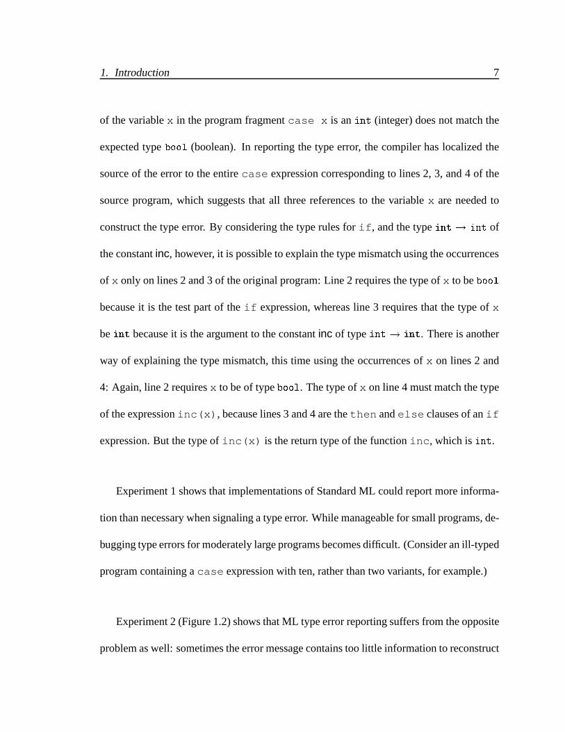
experiments. Experiment 1 (Figure 1.1) shows a simple program written in the 1998 New
Jersey dialect of Standard ML and the compiler’s messages reporting a type error. The body
of the function consists of a simple if expression containing three references to a bound
variable x (one each on lines 2, 3 and 4), and a predefined constant inc assumed to be of
type int ! int (line 3). The inexperienced ML programmer might find the error message
confusing. The confusion is exacerbated by the compiler converting the if expression into
a case expression along the way.2 The type error in this case has been triggered by the
unsuccessful attempt to unify int with bool. According to the error message, the type
2ML treats if as a macro. Tracking the source of errors in the presence of macros and rewriting systemsis the subject of a related, but separate study (see, for example, the work on origin tracking [10, 104]).
1. Introduction 7
of the variable x in the program fragment case x is an int (integer) does not match the
expected type bool (boolean). In reporting the type error, the compiler has localized the
source of the error to the entire case expression corresponding to lines 2, 3, and 4 of the
source program, which suggests that all three references to the variable x are needed to
construct the type error. By considering the type rules for if, and the type int ! int of
the constant inc, however, it is possible to explain the type mismatch using the occurrences
of x only on lines 2 and 3 of the original program: Line 2 requires the type of x to be bool
because it is the test part of the if expression, whereas line 3 requires that the type of x
be int because it is the argument to the constant inc of type int ! int. There is another
way of explaining the type mismatch, this time using the occurrences of x on lines 2 and
4: Again, line 2 requires x to be of type bool. The type of x on line 4 must match the type
of the expression inc(x), because lines 3 and 4 are the then and else clauses of an if
expression. But the type of inc(x) is the return type of the function inc, which is int.
Experiment 1 shows that implementations of Standard ML could report more informa-
tion than necessary when signaling a type error. While manageable for small programs, de-
bugging type errors for moderately large programs becomes difficult. (Consider an ill-typed
program containing a case expression with ten, rather than two variants, for example.)
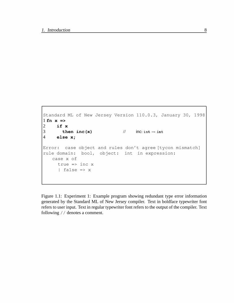
Experiment 2 (Figure 1.2) shows that ML type error reporting suffers from the opposite
problem as well: sometimes the error message contains too little information to reconstruct
1. Introduction 8
Standard ML of New Jersey Version 110.0.3, January 30, 19981 fn x =>2 if x3 then inc(x) // inc: int! int
4 else x;
Error: case object and rules don’t agree [tycon mismatch]rule domain: bool, object: int in expression:
case x oftrue => inc x| false => x
Figure 1.1: Experiment 1: Example program showing redundant type error informationgenerated by the Standard ML of New Jersey compiler. Text in boldface typewriter fontrefers to user input. Text in regular typewriter font refers to the output of the compiler. Textfollowing // denotes a comment.
1. Introduction 9
Standard ML of New Jersey Version 110.0.3, January 30, 19981 fn (f,g,x) =>2 if f(g(x)) then3 let val v = f(x)4 in g(v) end5 else6 let val z = g(x)7 in inc(z) end;
Error: case object and rules don’t agree [tycon mismatch]rule domain: bool, object: int in expression:
case f(g(x)) oftrue => let val <pat> = <exp> in g(v)| false => let val <pat> = <exp> in inc(z)
Figure 1.2: Experiment 2: Example program showing insufficient type error informationgenerated by the Standard ML of New Jersey compiler. Text enclosed in angle brackets ofthe error message denotes program parts deemed unnecessary for the reconstruction of theerror by the compiler.

1. Introduction 10
the type error. The program in Experiment 2 is ill-typed and its untypability may be ex-
plained by the following sequence of inferences. From line 2, we can infer that the return
type of f is bool. By lines 3 and 4, the type of v, which is an argument of g, is also bool.
Hence, the argument type of g is bool. Now, from lines 6 and 7, we can infer that the
return type of g is int. From this, and the application f(g(x)) on line 1, it is clear that
the argument type of f is int. Thus f has type int ! bool and g has type bool ! int.
The variable x being passed to f (line 3) is therefore of type int. This clashes with the
type bool required of x when it is passed to g in line 6.
The error message correctly identifies a “clash” between int and bool. Additionally,
the compiler suggests that the two let binding clauses (lines 3 and 6) are irrelevant to the
reconstruction of the type error. However, without using the type constraints gathered from
these two clauses, it is impossible to reconstruct the type error.
Haskell[50] is another popular functional programming language with a powerful type
inference system. When run under Haskell, the above experiments produce even more
inscrutable error messages, mainly due to the additional complexity of the type inference
introduced by Haskell’s overloading mechanism.
These experiments suggest a basic problem with the practical usability of type-inference-
based functional programming languages. Merely dressing up error messages produced by
existing compilers with a graphical user interface will only be of limited value. Instead,
useful error reporting requires integrating the generation of diagnostic information with the

1. Introduction 11
type inference process. A rigorous foundation for diagnosis of type errors should construct
formal proofs of untypability, because inferring the type or untypability of a program is, in
a technical sense, equivalent to proving a theorem. Therefore, error diagnoses should cor-
respond to proofs of untypability in an appropriate logic. Since type inference is based on
term-unification, it should be possible to reconstruct a proof of the type error starting from
the symptom of the type error, which is unification failure. These ideas of a proof-based
framework are illustrated in the next section where we analyze the program of Experiment 1
in more detail.
1.3.1 Diagnostic analysis of the program in Experiment 1
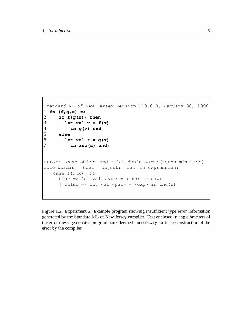
We show the type inference process involved in trying to infer the type of Experi-
ment 1’s example program, which we call e:
� x: if x (@ incint!int x) x
We use an abstract syntax based on �-calculus, replacing ML’s fn keyword with �, dis-
pensing with the keywords then and else, and denoting function application with @.
incint!int denotes the constant inc annotated with its type. The parse tree for e is given
in Figure 1.3. Each vertex in the parse tree corresponds to a location in e and is identified
with an integer. The parse tree of e may alternatively be specified using a set of syntax
1. Introduction 12
lambda
xif
x
@
inc x
0
1 2
34
5
6 7
x
int−>int
Figure 1.3: Parse tree of example program e of Experiment 1
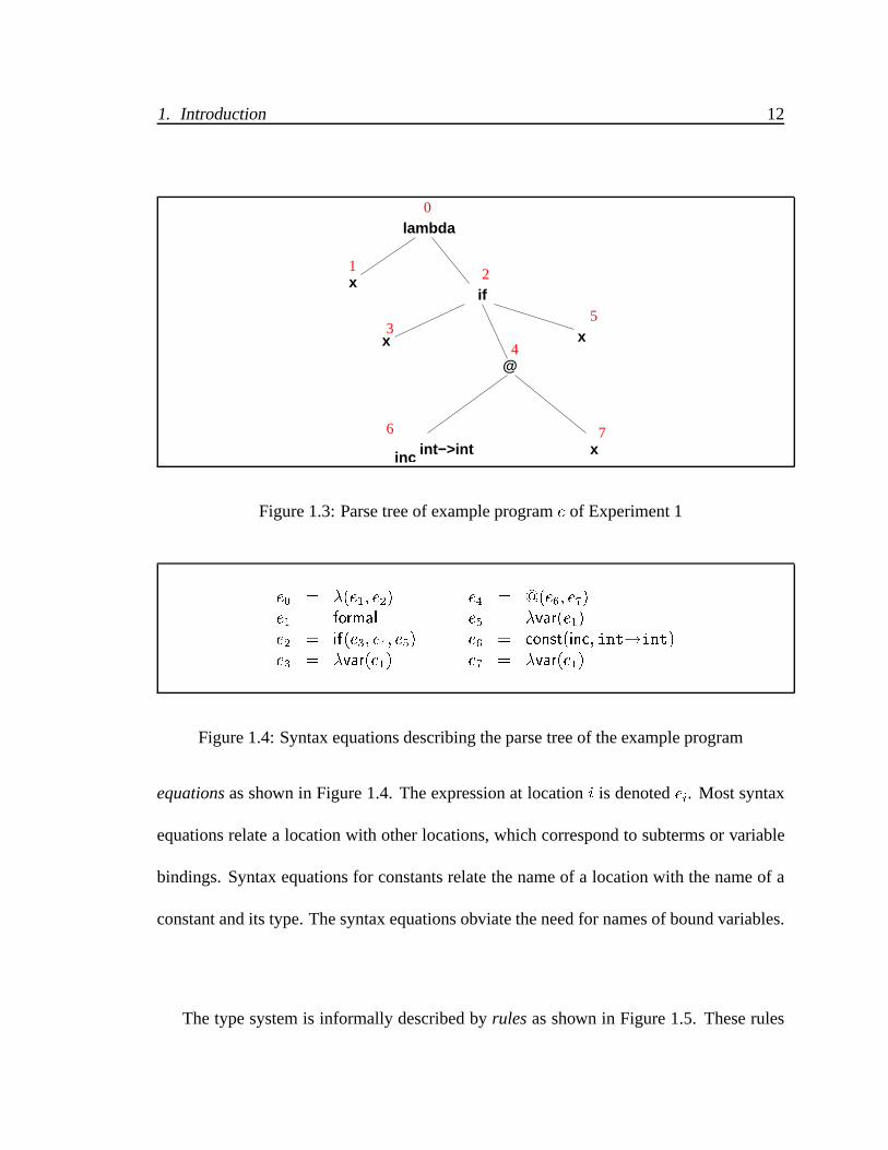
e0 = �(e1; e2) e4 = @(e6; e7)e1 = formal e5 = �var(e1)e2 = if(e3; e4; e5) e6 = const(inc; int!int)e3 = �var(e1) e7 = �var(e1)
Figure 1.4: Syntax equations describing the parse tree of the example program
equations as shown in Figure 1.4. The expression at location i is denoted ei. Most syntax
equations relate a location with other locations, which correspond to subterms or variable
bindings. Syntax equations for constants relate the name of a location with the name of a
constant and its type. The syntax equations obviate the need for names of bound variables.
The type system is informally described by rules as shown in Figure 1.5. These rules
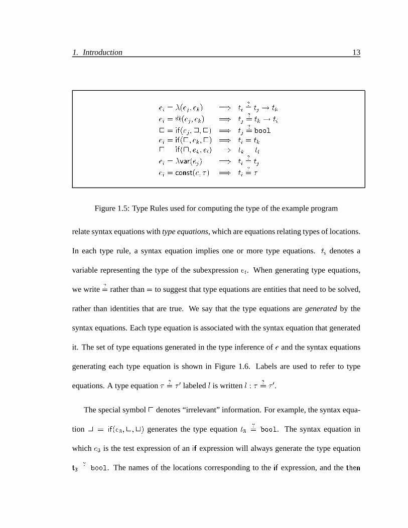
1. Introduction 13
ei = �(ej; ek) =) ti?= tj ! tk
ei = @(ej; ek) =) tj?= tk ! ti
2 = if(ej;2;2) =) tj?= bool
ei = if(2; ek;2) =) ti = tk2 = if(2; ek; el) =) tk = tl
ei = �var(ej) =) ti?= tj
ei = const(c; �) =) ti?= �
Figure 1.5: Type Rules used for computing the type of the example program
relate syntax equations with type equations, which are equations relating types of locations.
In each type rule, a syntax equation implies one or more type equations. ti denotes a
variable representing the type of the subexpression ei. When generating type equations,
we write ?= rather than = to suggest that type equations are entities that need to be solved,
rather than identities that are true. We say that the type equations are generated by the
syntax equations. Each type equation is associated with the syntax equation that generated
it. The set of type equations generated in the type inference of e and the syntax equations
generating each type equation is shown in Figure 1.6. Labels are used to refer to type
equations. A type equation � ?= � 0 labeled l is written l : � ?
= � 0.
The special symbol 2 denotes “irrelevant” information. For example, the syntax equa-
tion 2 = if(e3;2;2) generates the type equation t3?= bool. The syntax equation in
which e3 is the test expression of an if expression will always generate the type equation
t3?= bool. The names of the locations corresponding to the if expression, and the then
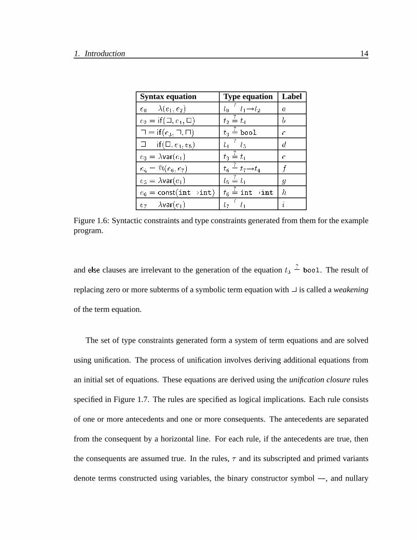
1. Introduction 14
Syntax equation Type equation Label
e0 = �(e1; e2) t0?= t1!t2 a
e2 = if(2; e4;2) t2?= t4 b
2 = if(e3;2;2) t3?= bool c
2 = if(2; e4; e5) t4?= t5 d
e3 = �var(e1) t3?= t1 e
e4 = @(e6; e7) t6?= t7!t4 f
e5 = �var(e1) t5?= t1 g
e6 = const(int!int) t6?= int!int h
e7 = �var(e1) t7?= t1 i
Figure 1.6: Syntactic constraints and type constraints generated from them for the exampleprogram.
and else clauses are irrelevant to the generation of the equation t3?= bool. The result of
replacing zero or more subterms of a symbolic term equation with 2 is called a weakening
of the term equation.
The set of type constraints generated form a system of term equations and are solved
using unification. The process of unification involves deriving additional equations from
an initial set of equations. These equations are derived using the unification closure rules
specified in Figure 1.7. The rules are specified as logical implications. Each rule consists
of one or more antecedents and one or more consequents. The antecedents are separated
from the consequent by a horizontal line. For each rule, if the antecedents are true, then
the consequents are assumed true. In the rules, � and its subscripted and primed variants
denote terms constructed using variables, the binary constructor symbol !, and nullary
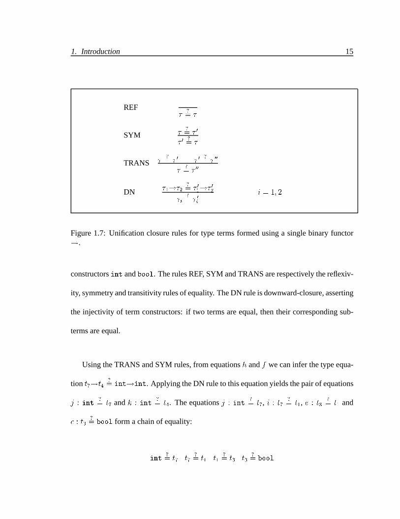
1. Introduction 15
REF�
?= �
SYM �?= � 0
� 0?= �
TRANS �?= � 0 � 0
?= � 00
�?= � 00
DN �1!�2?= � 01!� 02
�i?= � 0i
i = 1; 2
Figure 1.7: Unification closure rules for type terms formed using a single binary functor!.
constructors int and bool. The rules REF, SYM and TRANS are respectively the reflexiv-
ity, symmetry and transitivity rules of equality. The DN rule is downward-closure, asserting
the injectivity of term constructors: if two terms are equal, then their corresponding sub-
terms are equal.
Using the TRANS and SYM rules, from equations h and f we can infer the type equa-
tion t7!t4?= int!int. Applying the DN rule to this equation yields the pair of equations
j : int?= t7 and k : int
?= t4. The equations j : int
?= t7, i : t7
?= t1, e : t3
?= t1 and
c : t3?= bool form a chain of equality:
int?= t7 t7
?= t1 t1
?= t3 t3
?= bool
1. Introduction 16
implying int?= bool, which is clearly unsolvable. Also, the equations k : int
?= t4,
d : t4?= t5, g : t5
?= t1, e : t3
?= t1 and c : t3
?= bool form the chain
int?= t4 t4
?= t5 t5
?= t1 t1
?= t3 t3
?= bool
again yielding the unsolvable equation int?= bool.
The type constraints generated by the example program are unsolvable because together
they imply the unsolvable type constraint int ?= bool. Therefore, the example program
is untypable, or ill-typed, because the type constraints it engenders are unsolvable. We say
that the unsolvable type constraint int ?= bool is a symptom of the untypability of e.
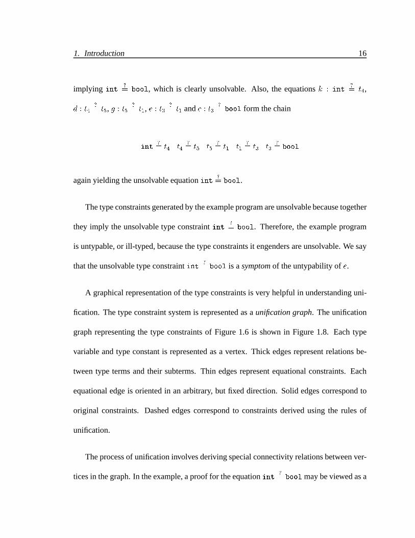
A graphical representation of the type constraints is very helpful in understanding uni-
fication. The type constraint system is represented as a unification graph. The unification
graph representing the type constraints of Figure 1.6 is shown in Figure 1.8. Each type
variable and type constant is represented as a vertex. Thick edges represent relations be-
tween type terms and their subterms. Thin edges represent equational constraints. Each
equational edge is oriented in an arbitrary, but fixed direction. Solid edges correspond to
original constraints. Dashed edges correspond to constraints derived using the rules of
unification.
The process of unification involves deriving special connectivity relations between ver-
tices in the graph. In the example, a proof for the equation int?= bool may be viewed as a
1. Introduction 17
bool
0 .. 7
w1 .. w5
strict vertices
functor vertices
1
2
3
4
5
6
7
m np
e
c
i
g
b
f ha
j
kd
q
sr
branch edges
equational edges
derived edges
paths
w1 w2 w3
w4
w5
0
num
Figure 1.8: Unification graph of example program. Each type variable ti is representedby the vertex i. Vertices with circles represent type constructors, with the label inside thecircle denoting the constructor symbol. Bold edges represent branch edges. Thin edgesrepresent equational edges. Dashed edges represent derived equations.
1. Introduction 18
path connecting the nodes int and bool in the unification graph, with the assumption that
directed and undirected edges may be traversed in either direction. Traversal of an edge y
opposite to its orientation is denoted y�1. Thus, the paths j�1ie�1c and k�1dge�1c between
the nodes int and bool in Figure 1.8 are both witnesses to the unsolvability of the system
of type equations, and thus the untypability of e. The edges j and k owe their existence
to the downward-closure rule and the connectivity of the ! nodes via the edges f and h.
Thus, the edge j is derived from the path p�1f�1hr consisting of edges specified by the
original set of type constraints. Similarly, the edge k is derived from the path q�1f�1hs.
The problem of diagnosing untypability can therefore be described as identifying a set
of original type constraints, or diagnosis, and through them a subsystem of syntactic infor-
mation from the program, or source that is sufficient to derive a particular type constraint.
In addition, we are interested in obtaining diagnoses of errors that are minimal with respect
to the weakening ordering. A diagnosis is minimal if it logically implies the symptom, but
no proper weakening of that diagnosis implies that symptom.
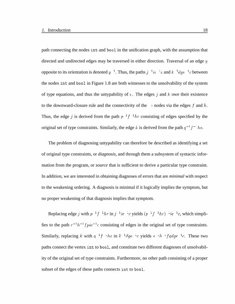
Replacing edge j with p�1f�1hr in j�1ie�1c yields (p�1f�1hr)�1ie�1c, which simpli-
fies to the path r�1h�1fpie�1c consisting of edges in the original set of type constraints.
Similarly, replacing k with q�1f�1hs in k�1dge�1c yields s�1h�1fqdge�1c. These two
paths connect the vertex int to bool, and constitute two different diagnoses of unsolvabil-
ity of the original set of type constraints. Furthermore, no other path consisting of a proper
subset of the edges of these paths connects int to bool.

1. Introduction 19
The set of edges fr; hg corresponds to the weakening t6?= int ! 2 of the constraint
h : t6?= int ! int. The 2 represents a “hole” indicating that the second occurrence
of int is irrelevant. Each occurrence of a hole is interpreted as an occurrence of a “new”
variable not occurring anywhere else in the set of equations. Similarly, ff; pg corresponds
to the weakening t6?= t7 ! 2 obtained by replacing the subterm t4 with 2 in the type
equation f : t6?= t7 ! t4. The path r�1h�1fpie�1c consisting of the two path segments
r�1h and fp, along with the edges i, e and c, therefore, correspond to the following set E1
of minimally non-unifiable type equations:
t6?= int! 2 t6
?= t7 ! 2
t7?= t1 t3
?= t1
t3?= bool
For each ti that is replaced with a 2 in the type equation, we replace the corresponding
occurrence of ei in the syntax equation with a 2. This yields the following set S1 of syntax
1. Introduction 20
equations that generate the type equations in E1:
e6 = const(2; int!2) =) t6?= int! 2
2 = @(e6; e7) =) t6?= t7 ! 2
e7 = �var(e1) =) t7?= t1
e3 = �var(e1) =) t3?= t1
2 = if(e3;2;2) =) t3?= bool
Similarly, the set of minimally non-unifiable type equations E2 derived from the path
s�1h�1fqdge�1c and the set of syntax equations, S2, generating E2 are:
e6 = const(2;2!int) =) t6?= 2! int
t4 = @(e6;2) =) t6?= 2! t4
2 = if(2; e4; e5) =) t4?= t5
e5 = �var(e1) =) t5?= t1
e3 = �var(e1) =) t3?= t1
2 = if(e3;2;2) =) t3?= bool
The syntax equation sets S1 and S2 are represented graphically in Figures 1.9(a) and
(b) respectively. The graphical representation consists of fragments of the parse tree ob-
tained by selectively erasing location information, or entire subtrees, from the parse tree.

1. Introduction 21
lambda
x1
if
x3
@
x6 7
int−> _
lambda
x1
if
x3
if
@
x
5
6
4
_−>int
(a) (b)
Figure 1.9: Graphical representation of syntax equations S1 and S2
The fragments are to be treated as patterns that match various subparts of the program ex-
pression’s parse tree. For example, there are two different if fragments in S2 that are both
matched by the same if subexpression of e. Besides e, any program whose syntax matches
the templates of S1 or S2 is also guaranteed to be ill-typed for the same reason as e.
The syntax equation sets S1 and S2 are minimal in the sense that any further weakening
of them will result in a set of type equations not constrained enough to generate a type
error.
1.4 Contributions of the thesis
This thesis is based on the premise that a rigorous diagnosis of type inference is possible
only after building a framework for diagnosis of term unification which is at the core of type
inference. The thesis identifies the three elements of a formal framework for term unifica-
tion: a graph-theoretic model for the unification diagnosis problem; a logical framework
to derive diagnostic information, and a practical algorithm for deriving source-tracking
1. Introduction 22
information in the event of unification failure.
Our framework for source-tracking term unification rests on fundamental properties re-
lating paths in labeled directed graphs to paths in their quotient graphs. By suitably labeling
the edges of the unification graph, we obtain a characterization of witnesses to membership
in the unification closure as paths whose labels form an important class of context-free lan-
guages, the semi-Dyck sets. There are advantages of thinking of unification closure purely
in terms of connectivity via these special paths, independent of the operational details of
any unification algorithm. For example, computation of optimal proofs reduces to search-
ing for optimal (shortest) paths. We define a logic PU(G) of connectivity over a labeled
directed graph G. We present the logic as a simple type system whose well-typed expres-
sions correspond to paths labeled with semi-Dyck set prefixes. We next define a practical
algorithm for deriving source-tracking information for unification. When the algorithm ter-
minates with failure, it also returns a proof of why the terms did not unify. The algorithm is
obtained by redefining standard unification algorithms to include an extra “proof” param-
eter. Next, using a rewrite system for groups, we simplify these proofs in order to identify
and remove details not relevant to the simulation of the error. The logic PU(G) has similar
soundness and completeness properties as the unification logic LE0 of Le Chenadec [64],
but is adapted to work on graph vertices so as to make the sharing properties of terms
explicit. A comparison of the two logics is detailed in Chapter 2.
We next consider the problem of error reconstruction for the classical Curry-Hindley

1. Introduction 23
type system of the simply-typed lambda calculus. Our formalization is based on viewing
the abstract syntax tree of a program as a set of syntax equations. Remarkably, this sim-
ple representation of program syntax is sufficient to define a precise constraint generating
function from syntactic equations to type constraints for the Curry-Hindley type system.
Prototype versions of the unification source-tracking algorithm and diagnostic type in-
ference for the Curry-Hindley type system have been implemented in Scheme [20].
Our approach for error diagnosis in unification and type inference is both more rigorous
and simpler compared to many existing approaches reviewed in Chapter 2.
1.5 Organization of the thesis
The rest of the thesis is organized as follows: Chapter 2 discusses several previous
attempts at addressing the diagnosis problem in various related contexts including type
inference, program debugging, logic programming, and Artificial Intelligence. Chapter 3
reviews the main definitions and results of term unification of rational terms. Unification
is treated as construction of closure relations on the vertices of a unification graph. Chap-
ter 4 presents a logical deduction system for computing proofs of non-unifiability. These
logical deductions are shown to correspond to typed path expressions in an algebra of un-
typed edge-expressions over the unification graph. Normalization in the untyped algebra is
1. Introduction 24
shown to preserve the types of these path expressions and thus forms the basis for remov-
ing redundancies from proofs. The practical outcome of this analysis is an extension of the
unification algorithm that supports automatic proof construction. Chapter 5 presents the
problem of diagnosing type errors in the Curry-Hindley type system. A framework based
on syntax and type equations is formally defined. Chapter 6 concludes the thesis with a
discussion of future extensions of the work on source-tracking to other other variants of
the unification problem, to more sophisticated type regimes, such as polymorphism in ML,
and finally to other problems such as debugging in logic programming languages.
2
Related Research
In this chapter, we survey research work specifically devoted to the type error and unifi-
cation failure diagnosis problem, and also work in other related areas, like program slicing,
logic programming, unification logics, and diagnosis in artificial intelligence.
2.1 Type Error Diagnosis: Previous attempts
This section catalogues previous attempts at solving the type error diagnosis problem
and their varying degrees of success.
2.1.1 Wand’s algorithm
Wand [108] was among the earliest to address the problem of reporting type errors. He
provided an implementation of his error diagnosis algorithm within the framework of his
25

2. Related Research 26
Semantic Prototyping System [107]. Wand’s algorithm was also used as an error reporting
front-end for the Infer system [43]. Wand’s algorithm is a modification of the structure
sharing version of the unification algorithm. It is based on the observation that Milner’s
polymorphic type inference algorithm [75] assigns a type variable to every lexically-bound
variable and every application. A unification inference tv:= � unifying a type variable
tv with a type expression � is called a type variable binding. A reason is a program site,
typically a function application. Reasons are accumulated when traversing the binding
pointers maintained by the unification algorithm. When a new binding from a type variable
tv to another type expression te is made, the reasons associated with this binding are defined
to be the set of reasons accumulated while arriving at the vertex representing te in the
unification graph.
With each pair of vertices u and u0 being unified, two sets of reasons r and r0 are
maintained. Intuitively, r is the set of reasons why the unifier arrived at vertex u, and r0
is the set of reasons why the unifier arrived at u0. If unification fails when trying to unify
u with u0, Wand’s algorithm simply returns the two sets of reasons at the point of failure.
Wand counts the algorithm as “successful in identifying the source of an error if the place of
the [error] was one of the error sites produced by the algorithm.” Wand also speculates the
existence of a ‘completeness criterion’ for judging the efficacy of his and other algorithms
that locate type errors. A plausible test for success is to verify if the reasons returned are
sufficient to reconstruct the error that is reported. Unfortunately, Wand’s algorithm fails this
2. Related Research 27
criterion even for some simple examples. Consider the following sequence of equations:
1 : x?= y, 2 : x
?= z. (The number preceding the colon indicates a source program
site.) Wand’s algorithm first performs the binding x 7! y, associating with it the reason
set f1g. The set of reasons accumulated following the binding pointers from x to y is
f1g, while the set of reasons accumulated following the binding pointers from z to z is fg,
because z is as yet unbound. When the the algorithm is ready to make the binding y 7! z,
it accumulates the reasons f1g to reach y from x, and the set fg as the reasons to reach
z. But, it unfortunately ignores the entire set of reasons accumulated for y when actually
making the binding. Instead, it only uses the reasons for reaching z to compute the reason
set for the binding y 7! z. (See the last four lines of the algorithm in Figure 1 of [108].)
Thus, y is bound to z, and the set of reasons attributed for this binding is fg. In other
words, the algorithm incorrectly concludes that neither of the premises x = y or x = z
are needed to infer the equation y = z. This bug can be easily fixed. There is one other
bug that causes more reasons to be lost. For example, given the sequence of unifications
1 : x?= y, 2 : x
?= int, 3 : x
?= bool, the error int ?
= bool will return the pair of reason
sets f1; 2g, obtained by traversing binding pointers from x to int, and fg, obtained from
traversing bool to bool. In order to simulate the error, we need the site 3 as well, which is
the site of the equation whose unification attempt resulted in the error. But this site is not
part of either reason list.
Another problem with the algorithm is that it generates redundant information even for
2. Related Research 28
simple inferences. In the example above, the set of reasons f1; 2; 3g together have enough
information to derive the error. But clearly, equation 1 is irrelevant to the derivation of the
error. Eliminating these redundant inferences from reason lists in a systematic way can
be done only by abandoning the algorithm’s set-based approach in favor of the path-based
approach of our algorithm. Furthermore, once all the relevant program sites are pointed out
as reasons, mentally reconstructing the chain of inferences from these sites can be difficult.
The approach we suggest is proof-based and automatically constructs a complete deduction
in a formal logic.
2.1.2 Attribute Grammars and flow information
Johnson and Walz [54, 106] formulate a theory of error correction and detection in
unification-based systems and apply it to the problem of unification-based type inference.
They view the process of type inference as attribute flow in the parse tree of the program,
reasoning that “type information is propagated up the expression tree1.” The other aspect
of information flow is the “propagation of completed constraint information about type
variables (including information about type errors) down the tree.” In the presence of type
errors, the “error information” field of each type variable collects all the conflicting types
of that variable along with a numerical “strength” with which the type variable is asserted
to have that type.
1page 47, [54]
2. Related Research 29
Type inference in the Johnson and Walz approach is based on the idea of “error-tolerant”
unification, which involves solving a multi-set of type constraints by considering disjunc-
tion rather than conjunction of constraints. For example, error-tolerant unification of the
constraint multi-set ft ?= bool; t
?= bool; t
?= intg yields t = int[1] j bool[2]. The solu-
tion suggests that t has the ‘options’ int and bool with indicated strengths. The Johnson
and Walz scheme rests on a complicated algorithm that derives implied type constraints
obtained from the original type constraints by applying the rules of substitution and transi-
tivity. Unfortunately, their work presents no soundness or completeness criterion to judge
the adequacy of their solution. Error-tolerant unification algorithm may be more useful in
type inference under “soft typing” regimes [16, 37] but the types returned by this approach,
specially in the presence of nested disjunctions, tend to be large and hard to understand.
The problem with the attribute grammar approach used by Walz and others [8, 35, 69]
is that these approaches confuse the generation of type constraints, which is directed by the
syntax of the program, with the solution of these constraints, which is instead directed by
the geometry of the constraints themselves, and not the parse-tree of the program. Type
information flows along specialized paths of the unification graph and not the parse tree.
2.1.3 Partial Type Inference
The goal of partial type inference is to infer as much type information as possible for
the ‘typable’ parts of the program and annotate the rest of the fragments of the program
2. Related Research 30
as ‘untypable’. Gomard [40] uses this idea to develop a type inference system essentially
based on a modification of Milner’s algorithm W. An ill-typed program is ‘well-annotated’
according to the rules of an extended type system that is permissive on the annotated (read
ill-typed) parts of the program and “imposes a ‘normal’ type discipline on the un-annotated
(type correct) parts.”
Gomard defines a notion of ‘completion’ between programs, where an expression e0 is
a ‘completion’ of e if e is well-annotated and is obtainable from e by adding annotations
to e. Gomard shows elsewhere that the set of expressions forming a completion of a given
expression e form a partial order. He speculates that his algorithm produces minimally
annotated completions of a program.
From the point of view of isolating and reporting type errors, Gomard’s approach does
not address one important question: what is the relation between the subexpressions of an
annotated expression that result in the type error? In fact, Gomard’s analysis makes no
attempt at using the actual type error (for example, whether the error was a type mismatch
of the form “int = bool” or an occurs check) in trying to diagnose the cause of the error.
Thus, Gomard’s technique offers at best an approximation of the result that we strive to
achieve: the relations between the subexpressions of the program that contribute to a type
error.
2. Related Research 31
2.1.4 Tracing Techniques
Maruyama et al. [69] propose a tracing and debugging front-end to the type inference
algorithm. The heart of their algorithm is a strategy for selecting a candidate set of ‘loca-
tions’ that correspond to the site of the type error. Their tracing technique for type error
analysis, however, is based on a flawed heuristic: only parse tree nodes that are adjacent
to the node where unification fails are considered. As demonstrated amply by our work,
more distant nodes may contribute to the error. It is necessary to consider adjacency in a
type-constraint graph rather than the parse tree. They provide no proof or even statement
about how the set of candidate error locations relates to the site of the error. Moreover,
the selection of a candidate location is done by the programmer using “his/her knowledge
about the program.” The work of Maruyama et al. uses a rudimentary slicing technique to
filter out irrelevant information from the trace of a type inference.
2.1.5 Explanation and Visualization-based systems
Most of the effort in debugging type error messages in ML has focused on providing
explanation-based and graphical front-ends for polymorphic type inference systems. Rela-
tively early efforts include Beaven and Stansifer [8], Duggan and Bent [35], Duggan [34],
and Soosaipillai [97]. In addition, the recent work of Yang and others [113, 114, 115, 116,

2. Related Research 32
117, 118] and Chitil [18] focuses on explanation-based and visual front-ends to polymor-
phic type error debugging.
The main effort in these attempts has been to develop an interface where the results
of all the type deductions (type bindings) are maintained carefully in the parse-tree of
the program. The interaction is prompted by the programmer using a protocol consisting
of three queries: Typeof, Why, and How. The Typeof query returns the type of an
expression or reports a type error if the expression is ill-typed. Typically, the type mismatch
occurs between an ‘expected type’ and the actually inferred type of a subexpression. At
this point, the Why query asks the system why it expects that a certain subexpression should
have a certain type. This essentially queries the system to display the ‘top-level’ rule of the
type discipline that was invoked while attempting to compute the type of the subexpression
in question. The query How navigates the type binding link pointers.
The principal drawback with the explanation-based approach is its lack of automation
or semantic basis for classifying valid paths. In contrast, the type error reporting framework
designed in this thesis provides the ability to automatically derive such an explanation in a
formal way, by producing a proof of untypability.
Several researchers (Beaven and Stansifer [8], Gomard [40], Johnson [54], Maruyama [69])
argue that the problem of type error detection and correction is especially difficult because
of polymorphic typing. Lee and Yi [65] propose a “top-down” version of the standard algo-
rithm of Milner [75]. They argue that their algorithm reports type errors more eagerly than
2. Related Research 33
Milner’s algorithm. Bernstein and Stark [9] propose a type system that assigns monomor-
phic types to free variables in ML expressions. They show how this may form the basis
of a practical system for debugging type errors. Yang et al. propose two incremental type
inference algorithms [114, 118] for computing the source of type errors in the presence of
polymorphism. A comparison of their type inference algorithms with those of Wand, John-
son and Walz, Lee and Yi, and Turner [102] can be found in Yang’s thesis [114]. However,
Yang’s algorithms do not derive formal proofs of untypability. Besides, these algorithms,
being built on top of unification, are unable to remove redundant inferences introduced by
unification.
While polymorphism significantly complicates the typing discipline, the difficulty of
reporting type errors is not primarily due to the demands of polymorphism. The funda-
mental difficulty in diagnosis of type errors is correctly formulating source-tracking in the
unification algorithms at the core of type inference, a premise also underlying the early
work in type error reporting [54, 108], and the more recent work of Gandhe et al. [38], and
McAdam [71, 72].
2.1.6 Program Slicing
Program slicing as a debugging technique gained prominence due to Weiser [110, 111].
There are several ways in which a program slice has been defined in the literature, (see for
example the survey chapter in Tip’s thesis [100]) but they all consider a program slice to

2. Related Research 34
be a subset of the program’s text and/or its execution profile (trace), i.e., a projection of
the sequence of the runtime state of the program that can simulate a given behavior of the
program. Program slicing has been effectively applied to derive dependency information
in data, control and other flow relations in program analysis and compilation tools. The
output of the diagnostic unification algorithm presented in this thesis may be considered as
a program slice of the unification graph.
The work of van Deursen [103, 104], Bertot [10], Tip [100] and others has focused on
a more formal approach to program slicing based on term rewrite systems. These works
of research address the problem of ‘origin tracking’ in term rewrite systems. Among the
interesting applications that their approach has been applied to consists of reporting error
messages in languages supporting type checking, but not type inference [30, 31, 32].
2.2 Logic Programming and unification-based systems
Logic programming and Prolog-based systems use unification as their underlying com-
putational engine. The problem of debugging logic programs consists of techniques to
manage and organize information about logic variable bindings obtained as a result of suc-
cessful unification, as well as undoing of bindings during unification failures. As the survey
by Ducasse and Noye [33] points out, a large number of logic programming environment
tools are based on abstract interpretation, algorithmic debugging, and tracing, but there is a

2. Related Research 35
surprising absence of application of program slicing techniques.
Both logic programming and type inference reduce to unification of term equations.
Failure analysis of unification in terms of identifying minimally unifiable subsets of term
equations was carried out by Port [89]. Port’s algorithm attempts to construct regular path
expressions over the unification graph. Our work shows that the path expressions of rele-
vance are a context-free set rather than a regular set.
Cox’s [25] idea of maximally unifiable subsets and minimally non-unifiable subsets has
also been employed as the basis for developing search strategies for breadth first resolution
of logic programs. Chen et al. [17] propose an algorithm to construct these subsets in con-
junction with the unification algorithm. Their algorithm works by explicitly maintaining
the unification closure relation as an auxiliary graph. The vertices of this graph are elements
of the unification closure relation of the original graph. Each inference is represented by
edges from the antecedent(s) to the consequent. Attached to each node is the subset of
equation used to derive the membership of a particular element in the unification closure.
Our extension to the unification algorithm keeps track of information that is more pre-
cise because it computes finer subsystems of the original set of term equations. Further-
more, the information maintained statically (as vertices) in the auxiliary graph constructed
by the algorithm of Chen et al. can be generated dynamically in our extension to the uni-
fication algorithm, implying that the space requirements of our algorithm is likely more
modest.

2. Related Research 36
Gandhe et al. [38] apply Cox’s idea of isolating maximally unifiable sets to the prob-
lem of correcting type errors in the Curry Hindley type system. Each maximally unifiable
set then corresponds to a set of constraints on the syntax of the original term. Candidate
corrections to the original untyped term are derived from maximally unifiable subsets by
constructing structures, called “sharing graphs,” originally used by Lamping to represent
�-calculus terms for optimal �-calculus reduction [60]. Their main result is a one-to-one
correspondence between constraints developed by Wand’s Type Inference algorithm [109]
and sharing graphs. McAdam [70] is another proposal for graph-based approaches to this
problem. Our work shows that generated type constraints can be put in a one-to-one corre-
spondence with flat syntax equations without requiring additional machinery for represen-
tation.
2.3 Unification Logics of Le Chenadec
Le Chenadec [62, 63, 64] introduces an equational logic for unification and notes the
potential use of his logics for diagnosing type inference. The objects of his logic are well-
founded terms and contexts. On the other hand, the logic PU , introduced in Chapter 4, is a
logic of connectivity of graph vertices. The soundness and completeness properties of PU
with respect to the unification graph are simpler to state and prove than those obtained from
the logic LE0 of Le Chenadec. (Compare, for example, Theorem 4.3.1 and Lemma 4.4.1

2. Related Research 37
in Chapter 4 with Proposition 2.10 in [64].) All assumptions about the sharing structure
are explicit in the logic PU , whereas LE0 depends on restricting subterm sharing only to
strict variables ([64], page 151). The group theoretic framework proposed in this thesis
for simplifying path expressions is a special case of the more general homotopy algebra
semantics for unification deductions proposed by Le Chenadec. This specialization is all
that is needed to reduce non-unifiability to the existence of context-free paths. The path-
oriented view of proofs of membership in the unification closure allows us to characterize
the problem of computing optimal unification diagnosis as a path minimization problem.
The specialization to free groups also results in a simple algorithm for removing some,
but not all, redundancies in non-unifiability proofs. A useful exercise would be to com-
pare the quality of the proofs thus obtained with the variety of confluent rewrite systems
introduced by Le Chenadec that operating directly on deductions. It is unlikely that his
rewrite systems would yield shortest proofs or even minimal proofs. On the other hand,
our framework affords the choice of computing non-optimal paths relatively cheaply (con-
stant overhead to the unification algorithm), or computing optimal paths more expensively
(in time polynomial in the size of the unification graph).

2. Related Research 38
2.4 Diagnosis in Artificial Intelligence
Explanation-based diagnosis has always been an important issue in AI (Reiter [90],
deKleer[29], Wick and Thompson [112], Genesereth [39]). Reiter, de Kleer and oth-
ers [29, 90] develop a general characterization of system-description, behavior, conflict
and diagnosis based on propositional logic. Reiter formulates broad criteria for model-
based generation of diagnostic information based on the idea of “minimally conflicting
sets.” This notion of minimality is used in our framework for untypability in Chapter 5.
3
A review of term unification
The problem of term-unification is concerned with solving equations of terms over
abstract algebras. The main components of the formal treatment of unification are the
data structures of unification (terms and unification graphs), operations over these data
structures (substitutions, solutions, unifiers, and most general unifiers), and relations overs
these data structures (term-bisimulations, downward-closed equivalences and unification
closures).
The formalism presented in this chapter addresses the unification of finite and circular
terms, collectively known as rational terms. The problem of unification over rational terms
was first studied by Huet [51]. Other studies of unification for infinite terms, for example
Jaffar [53], Mukai [80], and Colmeraur [22], have been concerned more with developing
efficient algorithms rather than building formalisms. Rational terms have been defined
as infinite trees using metric spaces and complete partial orders (Courcelle [24]). In this
39
3. A review of term unification 40
chapter, they are modeled as non-wellfounded sets (Aczel [1]) obtained as solutions to flat
systems of set equations (Barwise and Moss [6]).
The simplest variant of the unification problem, known as unification in the empty
theory, consists of equations over inductive terms. Solutions, or unifiers of equations of
wellfounded terms, may however result in unifiers whose range includes non-wellfounded
terms.1 When considering the unification problem for rational terms, all the main re-
sults, including conditions for the existence of unifiers and properties of most general
unifiers, continue to hold. However, terms, equality, and substitutions need to be defined
co-inductively rather than inductively, and this requires a reworking of the proofs of the
basic results.
The origins of the unification problem can be traced to the 1930’s in the work of Her-
brand [45]. In the 1960’s, Robinson coined the term “unification” and showed how it lay
at the heart of resolution-based theorem proving [91]. Robinson defined the notion of
a most general unifier and proposed an algorithm for computing mgu’s. Since then, the
properties of substitutions and unifiers have been studied extensively (Eder [36], Lassez et
al. [61]). Furthermore, the many variants and generalizations of the unification problem
(E-unification, higher-order unification, semi-unification etc.) and its diverse applications
to areas of theorem proving, artificial intelligence, databases, type inference, and logic
programming (Prolog) has since spawned a vast area of research. Surveys of unification,
1Enabling non-wellfounded solutions is done by removing the so-called “occurs-check” in unificationimplementations.

3. A review of term unification 41
including its applications in other areas can be found in Knight [59], and Baader and Siek-
mann [3].
The formalism presented here emphasizes the relational basis of the unification prob-
lem and its solution, as in Le Chenadec [64], Baader and Siekmann [3], and Paterson and
Wegman [84], rather than the transformational approach of Martelli and Montanari [68],
Lassez et al. [61], and Jouannaud and Kirchner [55]. The relational approach casts uni-
fication in terms of connectivity properties of the graph data structures representing the
unification problem. The connectivity properties are crucial to constructing a proof theory
of unification and the integration of unification proofs into existing unification algorithms.
Section 1 presents the basic definitions, including that of �-graphs, the underlying data
structure used to model terms. Section 2 defines rational terms as co-inductive types. Sec-
tion 3 defines of the notion of substitution over rational terms. Section 4 lays out the unifi-
cation problem and its solution, including unifiability, unification closure, and the compu-
tation of most general unifiers.

3. A review of term unification 42
3.1 Basic Definitions
3.1.1 Relations
Given sets A and B, a (binary) relation R over hA;Bi is a subset of A � B. We write
aRb to denote (a; b) 2 R. When A = B, we say R is a relation over A. A relation R over
a set A is reflexive if aRa for each a 2 A. R is symmetric if for all a; b 2 A, aRb implies
bRa. R is transitive if for all a; b; c 2 A, aRb and bRc implies aRc. R is an equivalence
if R is reflexive, symmetric and transitive. For each v 2 A, [v]R denotes the equivalence
class of R that contains v. When the equivalence is clear from context, [v]R is abbreviated
[v]. R is non-wellfounded if there is an infinite sequence a0; a1; : : : of elements of A such
that ai+1Rai for each 0 � i. The sequence a0; a1; : : : is called a descending sequence
for R starting at a0. If there is no such sequence, then R is wellfounded. R is cyclic, or
circular, if there is a finite sequence a0; : : : an, such that a0 = an and ai+1Rai, for each
0 � i � n � 1. Such a sequence is called a cycle for R starting at a0. Clearly, if R is
circular then it is non-wellfounded. For example, the relation <, denoting “less than” on
natural numbers is wellfounded, but > denoting “greater than” is non-wellfounded.
If R is a relation over a set A, then the transitive closure of R, denoted R+, is the least
transitive relation containing R. The reflexive transitive closure of R, denoted R�, is the
least reflexive, transitive relation containing R. It is easy to verify that a relation R on A is
cyclic if and only if for some a 2 A, aR+a.
3. A review of term unification 43
g : A �! B denotes a (total) function g from the set A to set B. If S � A, then g[S],
the image of g on S is the set fg(x) j x 2 Sg. If f : A �! B and g : B �! C, then
g � f : A �! C, also written gf , is the function defined as g(f(x)) for each x 2 A. For
each set A, IA denotes the identity function on A defined as IA(x) = x for each x 2 A.
3.1.2 Directed Graphs
A directed graph is a pair G = hV;Di, where V is a set of vertices and D � V � V
is a set of directed edges. The pair (u; v) 2 D is written u �! v and represents an edge
from u to v. u and v are respectively the source and destination of the edge u �! v, and
are identified by the projection function src and dest respectively.
Given a directed graphG = hV;Di, the connectivity relations ��! and +
�! on V denote the
reflexive transitive closure and transitive closure, respectively, of the directed edge relation
D. We write G j= u �! v if u �! v 2 D. Similarly, we write G j= u��! v and
G j= u+�! v.
If G is a directed graph containing vertices u and v, then a path from u to v in G is a
finite, possibly empty sequence of directed edges c1 : : : cn, 0 � n, such that if 0 < n, then
for each 1 � i � n, ci 2 D, and dest(ci) = src(ci+1), and if n = 0, then u = v. If p is a
path, then the length of p, denoted jpj, is n. p is empty if jpj = 0. If p is a path from u to v,
then u and v are respectively the source and destination of p, and src(p) = u, dest(p) = v,
3. A review of term unification 44
and endpoints(p) = hu; vi.
It is easy to see that given a graph G, G j= u��! v if and only if there is a path from u
to v in G, and G j= u+�! v if and only if there is a non-empty path from u to v in G.
3.1.3 Alphabet, sentences, signature
We use N to denote the set of natural numbers. An alphabet � is a set whose elements
are called symbols. �� is the set of all finite sequences a1 : : : an such that n 2 N, and
ai; 1 � n 2 �. The elements of �� are called sentences over �. If l = a1 : : : an and
l0 = a01 : : : a0
m are sentences, then the sentence a1 : : : ana01 : : : a0
m denotes the concatenation
of l with l0. The empty sentence is denoted �, and l� = �l = l for every sentence l.
Clearly, concatenation is associative. A �-language , or language, is any subset of ��. The
language �+ denotes the set of non-empty sentences over �. �0 denotes the set f�g.
A binary relation R over �� is a congruence if for all sentences x; y; u; v over �, xRy
implies uxvRuyv. If p; q; r are sentences over � such that p = qr, then q is a prefix of p
and r is a suffix of p. A language L � �� is prefix closed (respectively suffix closed) if for
each p 2 L, every prefix (respectively suffix) of p is in L.
A signature is an alphabet � of functor symbols equipped with an arity function arity :
�! N. A signature � is usually specified by enumerating its arity function. For instance,
3. A review of term unification 45
ff 7! 2; a 7! 0g denotes a signature with functor symbols f and a with arity 2 and 0 re-
spectively. If arity(f) = n, we say f is n-ary. 0-ary functors are called constants. If � is
a signature, the alphabet �N = ffijf 2 �; 1 � i � arity(f)g is called the set of context
symbols of �. To avoid double subscripts, �N is sometimes written �:N and the label fi is
written f:i. For example, if � = ff 7! 2; g 7! 1; a 7! 0g, then �N = ff1; f2; g1g.
A tuple of size n 2 N over a set A is a function f0; : : : ; n� 1g �! A. A tuple p of
size n is written (a0; : : : ; an�1), or ha0; : : : ; an�1i. The size of a tuple p is denoted jpj. The
element p(0) is called the head of p and denoted hd(p). The tail of p, denoted tl(p), is a
tuple of size jpj � 1 defined as tl(p)(i) = p(i + 1), 0 � i < jpj � 1.
If A is a set, and � a signature, �(A) denotes the set
f(f; a1; : : : ; an) j f 2 �; arity(f) = n; a1; : : : ; an 2 Ag
The tuple (f; a1; : : : ; an) 2 �(A) is written f(a1; : : : ; an), and f() is abbreviated f .
3.1.4 Labeled directed graphs, �-graphs
Directed graphs often have labels associated with vertices or edges or both, giving rise
to labeled directed graphs. A labeled directed graph G is a tuple h�V ;�D; V; L;Di, where
�V and �D are a pair of alphabets, respectively called the vertex and edge labels sets of
G, L : V �! 2�V is a vertex labeling function and D � V � V � (�D [ f�g) is the set

3. A review of term unification 46
of labeled edges of G. The tuple hu; v; �i 2 D is written u ��! v. The source, destination
and label of u ��! v are respectively u, v and �, and are identified with the projection
functions src, dest and l. Edges whose labels are in �D are called branch edges. A vertex
u 2 V is strict if L(u) = ;. u is homogeneous if L(u) is either empty or a singleton. G
is homogeneous if every vertex in V is homogeneous. G is deterministic if for any two
edges w ��! u and w
��! v in G, u = v. G is guarded if for all u; v 2 V , u �
�! v
implies u = v. The underlying directed graph of G is the directed graph G0 = hV;D0i,
where D0 = fu �! vju��! v 2 D for some �g.
In a labeled directed graph G = h�V ;�D; V; L;Di with vertices u; v 2 V , a labeled
path or path from u to v over G is a possibly empty sequence c1 : : : cn, 0 � n of labeled
directed edges c1 : : : cn, 0 � n, such that if 0 < n, then for each 1 � i � n, ci 2 D, and
dest(ci) = src(ci+1), and if n = 0, then u = v. If p is a labeled path, then the label of p,
denoted l(p), is the sentence over �D obtained by concatenating the labels of each edge in
that path. If p is empty, then l(p) is defined to be the empty sentence �. We assume that
there is an empty path from every vertex to itself, and this empty path is also denoted �.
G j= p : ul
�! v denotes that p is a path from u to v labeled l in G. G j= ul
�! v denotes
that there is a path from u to v labeled l in G.
Let G = h�V ;�D; V; L;Di be a labeled directed graph, and let R be an equivalence
relation on V . R is downward-closed if, for each uRu0 and directed edges u ��! v 2
D and u0��! v0 2 D with the same label �, it is the case that vRv0. The quotient
3. A review of term unification 47
graph G=R of G is the labeled directed graph h�V ;�D; VR; LR; DRi where VR is the set
of equivalence classes of R, LR([u]R) = [fL(v) j v 2 [u]Rg for each equivalence class
[u]R of R containing the vertex u 2 V , and [u]R��! [v]R 2 DR if and only if there are
u0; v0 2 V such that uRu0, u0 ��! v 2 D, and v0Rv.
We now consider a special subclass of labeled directed graphs used for modeling terms
and equations between them. Let � be a signature. A �-graph is a labeled directed graph
G = h�;�N; V; L;Di with the restriction that G is deterministic and homogeneous, and,
if f:i 2 �N and uf:i�! v 2 D, then f 2 L(u). A �-graph h�;�N; V; L;Di is abbreviated
hV; L;Di. A � graph G is complete if for each vertex u in G, if f 2 L(u) and arity(f) = n,
then there are vertices u1; : : : un such that for each i, uf:i�! ui is an edge in G.
3.2 Rational Terms
A term is an algebraic expression built from symbols from a signature and a set of
variables. Common mathematical usage of the word “term” assumes that it is wellfounded,
that is, it can be defined bottom-up, starting from the variables and constants, and building
more complex terms using function symbols. More generally, however, terms, modeled as
non-wellfounded sets [1], could contain themselves as proper subterms. Such terms, called
rational terms, are useful for modeling circular data types like recursive environments,
objects, and processes. A rational term is a term with a finite, and possibly circular subterm
3. A review of term unification 48
relation. In order to understand the relationship between wellfounded and rational terms, it
is useful to define the set of �-terms in such a way as to include wellfounded, circular, and
non-wellfounded terms.
If � is a signature and V a set of strict variables disjoint from �, the set T1(�;V) of
�-terms over V, or terms, is defined as the largest fixed-point of the domain equation
T (�;V) = V + �(T (�;V)) (3.1)
Thus, a �-term is a strict variable, or a compound term � = f(�1; : : : ; �n), 0 � n, where
f 2 �, and �1; : : : ; �n are all �-terms. f is called the head of � . If � = f(�1; : : : ; �n), then
each �i, 1 � i � n, is the immediate subterm of � at position i. If � is a strict variable,
then the set of immediate subterms of � is ;. The proper subterm relation is the transitive
closure of the immediate subterm relation. The subterm relation is the reflexive, transitive
closure of the immediate subterm relation.
A �-term � is non-wellfounded if there is a descending chain for the immediate subterm
relation starting at � . Otherwise, � is wellfounded. � is circular if there is a cycle for the
immediate subterm relation starting at some subterm of � . Otherwise, � is non-circular. �
is rational if the set of its subterms is finite. Otherwise, it is irrational. Wellfounded terms
are also called inductive terms. The set of wellfounded �-terms overV, denoted T �(�;V),
is the least fixed-point of Equation 3.1. In other words, wellfounded terms are the least set

3. A review of term unification 49
such that each variable in V is a term, and if �i; : : : ; �n, 1 � n are terms and f 2 � and
arity(f) = n, then f(�i; : : : ; �n) is a term. The set of rational �-terms over V, denoted
T+(�;V), is also a fixed-point of Equation 3.1. It therefore includes the set of wellfounded
�-terms. The inclusion relation between the three fixed-points of Equation 3.1 is
T �(�;V) � T+(�;V) � T1(�;V)
The function vars : T (�;V) �! 2V maps a term to the set of all variables occurring in
that term. Clearly, if � is rational, vars(�) is finite.
Example 3.2.1: Let� = f(f; 1)g and V = fxg. Then T �(�; V ) = fx; f(x); f(f(x)); : : :g,
and T+(�; V ) = T1(�; V ) = T �(�; V ) [ ff(f(f(:::)))g. 3
Example 3.2.2: Let � = f(g; 1); (h; 1)g and let x 2 V . Then the terms x; g(x); h(x) and
g(h(x)) are all wellfounded. The term g(g(g(:::))) is circular, because it contains itself as
its (only) proper subterm. Let � be the term H1(H2(H3(:::))), where Hi is g or h depending
on whether the ith bit in the binary expansion of the number � is 0 or 1 respectively. Then
� is irrational. 3
For the rest of the discussion in this chapter, we assume the existence of a set V of
strict variables. The phrase “�-term” will refer to an element in T+(�;V). Properties of
�-terms and equations over these terms are the main objects of study in term unification.
3. A review of term unification 50
3.2.1 Flat Systems
Wellfounded terms are represented as finite trees or finite directed acyclic graphs (DAG’s).
Rational terms are represented as finite graphs. Wellfounded compound rational terms are
represented by a finite textual representation in the usual way: f(�1; : : : ; �n), for example.
Rational �-terms are identified as solutions of a finite system of equations. The equa-
tions consist of two disjoint sets of variables: the parameters of the system, which are
a finite subset of V, and the indeterminates of the system, which are also called functor
variables, and which are variables to which values are assigned. Therefore, a system of
equations is a function on indeterminates. Equations allow us to express circularity as well
as sharing of subterms. A system usually represents several terms at once. For example,
the terms � = f(g(x); �) and g(x) are represented by the system of equations shown below.
w = f(w0; w)
w0 = g(x)
The system of equations has one strict variable x and two functor variables w and w0. There
is one equation per functor variable, and each equation is flat: subterms are nested one-level
deep.
Notation: In this and the following chapters, strict variables will be denoted by x; y; z; t
etc., functor variables by w, variables (strict or functor) by u; v, functor variables by f; g; h

3. A review of term unification 51
etc., and terms by � . In addition, subscripted and primed variants of these symbols will
also be used.
Let � be an alphabet and V a set. Formally, a system of flat �-term equations , or flat
system over V , for short, is a tuple T = hW;X; bi, where X � V is a finite set of strict
variables, W is a finite set of indeterminates disjoint from V , and b : W ! �(X [W ) is
a set of flat equations. b(w) = f(u1; : : : ; un) is informally written as w = f(u1; : : : ; un).
The label of a functor variable w, denoted L(w), is the functor symbol hd(b(w)).
A pointed system of flat term equations, or pointed flat system, is a pair hv; T i, where
T = hW;X; bi is a flat system, and v 2 X [W . A pointed flat system provides a way to
refer to a particular subterm of a term represented as a flat system.
Every term � may be represented by a pointed flat system h�; T i, where T = hW;X; bi,
W is the set of compound subterms of � , X is the set of strict variables in � . If � 0; �1; : : : ; �n
are all subterms of � , and � 0 = f(�1; : : : ; �n), then b(� 0) = f(�1; : : : ; �n). Thus, for each
compound subterm of � , there is a flat equation in T .
A mapping s from W to �-terms is a solution of T if, for each w = f(u1; : : : ; un) 2 b:
s(w) = f(s(u1); : : : ; s(un)) (3.2)
where s(u) denotes u if u 2 X , and s(u) if u 2 W .
The Solution Lemma formulation of the Anti-Foundation Axiom [6] asserts that every
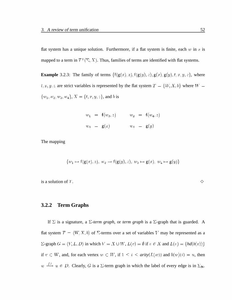
3. A review of term unification 52
flat system has a unique solution. Furthermore, if a flat system is finite, each w in s is
mapped to a term in T+(�; X). Thus, families of terms are identified with flat systems.
Example 3.2.3: The family of terms ff(g(x); z); f(g(y); z); g(x); g(y); t; x; y; zg, where
t; x; y; z are strict variables is represented by the flat system T = fW;X; bg where W =
fw1; w2; w3; w4g, X = ft; x; y; zg, and b is
w1 = f(w3; z) w2 = f(w4; z)
w3 = g(x) w4 = g(y)
The mapping
fw1 7! f(g(x); z); w2 7! f(g(y); z); w3 7! g(x); w4 7! g(y)g
is a solution of T . 3
3.2.2 Term Graphs
If � is a signature, a �-term graph, or term graph is a �-graph that is guarded. A
flat system T = hW;X; bi of �-terms over a set of variables V may be represented as a
�-graph G = hV; L;Di in which V = X [W , L(v) = ; if v 2 X and L(v) = fhd(b(v))g
if v 2 W , and, for each vertex w 2 W , if 1 � i � arity(L(w)) and b(w)(i) = u, then
wf:i�! u 2 D. Clearly, G is a �-term graph in which the label of every edge is in �N.
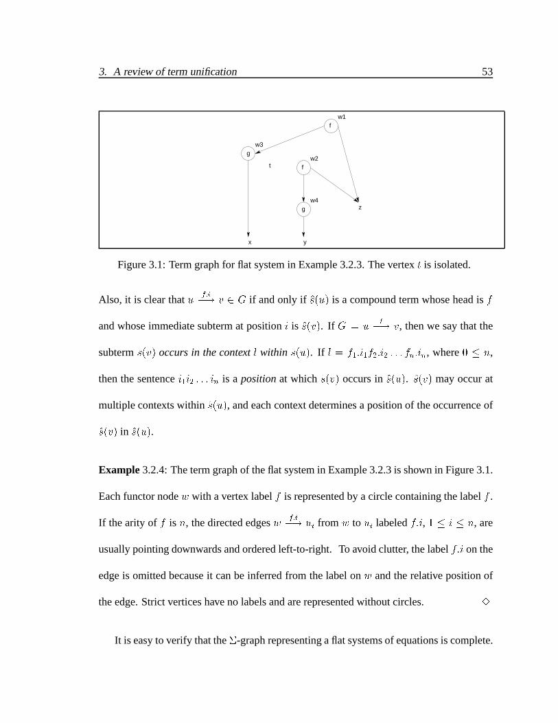
3. A review of term unification 53
f
f
gw2
w3
w4g
yx
w1
t
z
Figure 3.1: Term graph for flat system in Example 3.2.3. The vertex t is isolated.
Also, it is clear that uf:i�! v 2 G if and only if s(u) is a compound term whose head is f
and whose immediate subterm at position i is s(v). If G j= ul
�! v, then we say that the
subterm s(v) occurs in the context l within s(u). If l = f1:i1f2:i2 : : : fn:in, where 0 � n,
then the sentence i1i2 : : : in is a position at which s(v) occurs in s(u). s(v) may occur at
multiple contexts within s(u), and each context determines a position of the occurrence of
s(v) in s(u).
Example 3.2.4: The term graph of the flat system in Example 3.2.3 is shown in Figure 3.1.
Each functor node w with a vertex label f is represented by a circle containing the label f .
If the arity of f is n, the directed edges wf:i�! ui from w to ui labeled f:i, 1 � i � n, are
usually pointing downwards and ordered left-to-right. To avoid clutter, the label f:i on the
edge is omitted because it can be inferred from the label on w and the relative position of
the edge. Strict vertices have no labels and are represented without circles. 3
It is easy to verify that the �-graph representing a flat systems of equations is complete.

3. A review of term unification 54
�-term graphs that are not complete can be thought of as modeling “incomplete �-terms”
which may have some subterms missing. The missing subterms are often denoted by a hole
2. For example, the term f(2; g(2; a)) denotes an “incomplete �-term” with holes.
Flat systems and complete term graphs will be used interchangeably. Thus we write
T = hW;X; bi to denote a flat system and the complete term graph of T . But we will
sometimes work with �-term graphs that are incomplete.
3.2.3 Term-bisimulation
For wellfounded rational terms, equality can be defined using induction. In the pres-
ence of circularity, however, equality needs to be defined in terms of observational equiva-
lence, a notion introduced in the study of automata theory and the algebra of processes [76,
83]. For rational terms, the observation of interest is the possibly infinite, fully-expanded
printed representation of the term, where each functor variable is replaced by the right-
hand side of its defining equation. For example, if we have two equations satisfying
f� = f(� 0); � 0 = f(�)g both � and � 0 have the infinite printed representation f(f(f(:::))),
and therefore should denote the same term. The Extensionality Principle for wellfounded
terms states that two terms are equal if and only if they have the same outermost functor
symbol and their corresponding subterms are equal. However, if we use this principle to
prove � = � 0, we are lead to the vacuous reasoning � = � 0 if and only if � = � 0.
3. A review of term unification 55
Definition 3.2.1: Let � be a signature and V a set of variables. A term-bisimulation R
is a relation over T1(�; V ) such that for each (�; � 0) 2 R, one of the following term-
bisimulation condition holds:
1. � and � 0 are variables and � = � 0, or
2. � = f(�1; : : : ; �n) and � 0 = f(� 01; : : : ; �0
n), that is, the heads are the same, and for
each 1 � i � n, �iR� 0i .
� and � 0 are bisimilar if �R� 0 for some term-bisimulation R. 2
In the presence of rational terms, the Principle of Extensionality needs to be reformu-
lated using the notion of term-bisimulations.
Extensionality Principle for rational terms: Two terms � and � 0 are equal if and only if
they are bisimilar.
Proving the equality of non-wellfounded terms using the extensionality principle is re-
ferred to as proof by co-induction. The co-inductive proof for showing equality for rational
terms � and � 0 consists of (1) constructing a relation R, (2) proving that R is a term-
bisimulation, and (3) verifying that (�; � 0) belongs to R.
It is not hard to verify that =, the Equality relation over �-terms, is a term-bisimulation.
In fact, it is the largest term bisimulation. Therefore, in co-inductive proofs, it is convenient
to construct a relation R and verify that the relation R [ = is a term-bisimulation. Using

3. A review of term unification 56
this “stronger co-inductive” principle, after constructing a relation R, we verify that terms
in each pair of R are either equal, or satisfy the term-bisimulation condition.
Example 3.2.5: Consider the terms �1 = f(�1) and �2 = f(f(�2)). The relation R =
f(�1; �2); (�1; f(�2))g is a term-bisimulation. It is easy to verify that each pair (�1; �2) and
(�1; f(�2)) satisfies the term-bisimulation conditions: �1 and �2 are both compound terms,
their outermost functor symbols are identical, and their immediate subterms �1 and f(�2)
are related by R. Similarly, the outermost functor symbols of �1 and f(�2) are identical,
and their immediate subterms �1 and �2 are related by R. Hence, by co-induction, �1 = �2.
3
A general introduction to bisimulations, including a justification for the extensionality
principle for non-wellfounded sets, can be found in (Barwise and Moss [6]). A tutorial
presentation of co-induction in a co-algebraic framework is discussed in (Jacobs and Rut-
ten [52]).
3.3 Substitutions
Let � be a signature and V and V 0 be a sets of strict variables. A substitution s over
V is a mapping defined over a subset of V . The subset of variables over which s is de-
fined is called the domain of s and denoted dom(s). s maps each element of dom(s) to

3. A review of term unification 57
a �-term over V 0. The operation application of a substitution s to �-terms over V , de-
noted apply(s; ) and abbreviated s, is defined as the largest set satisfying the following
conditions:
1. if � 2 dom(s), then s(�) = s(�).
2. if � 2 V � dom(s), then s(�) = � .
3. if � = f(�1; : : : ; �n), then s(�) = f(s(�1); : : : ; s(�n))
The definition of s( ) on the domain of rational terms is an example of definition by
co-recursion. If the application operation were defined using induction (smallest set closed
under the above conditions), then its domain would include only the wellfounded �-terms
over V .
If s is a substitution over V and � 2 T+(�; V ), then s(�) is uniquely determined by
the values of s on vars(�). The set of variables occurring in s is denoted vars(s). The set
of independent variables in s, denoted ind(s), is the set of variables x in vars(s) such that
apply(s; x) = x. If V is a set of variables, and X � V , then any two substitutions s1 and
s2 on V agree on X if s1(x) = s2(x) for each x 2 X . This is abbreviated s1 =X s2. It is
easy to see that =X is an equivalence relation. It is easy to show that if s1 and s2 agree on
vars(�), then s1(�) = s2(�). Given a substitution s, and a set of variables X � dom(s),
the restriction s jX of s to the domain X denotes the substitution with domain X satisfying
the condition s jX (x) = s(x) for each x 2 dom(s).

3. A review of term unification 58
Given substitutions r over V 0 and s over V , their composition, written rs, is the sub-
stitution over V [ V 0 with domain dom(s) [ dom(r) satisfying the condition that for each
x 2 dom(s)[dom(r), (rs)(x) = r(s(x)). Composition is associative, so r(st) = (rs)t.2 A
substitution is idempotent if ss = s. The identity substitution, denoted I is the substitution
with an empty domain. It can be easily verified, that I(�) = � , for any �-term � , and
Ir = rI = r, for any substitution r.
3.4 Unification
We move from systems of flat equations to systems with a more general form of equa-
tions. A �-term equation over a set of variables V , or term equation is an unordered pair
�?= � 0 of rational �-terms over V . A system of �-term equations over V is a finite set of
�-term equations over V . If E is a set of term equations over V , a substitution s over V is a
unifier of E if s(�) = s(� 0) for each � ?= � 0 2 E . We say that s unifies E . s is a most general
unifier (mgu) of E if for every unifier s0 of E , s0 =V s0s. While flat systems always have so-
lutions, systems of term equations do not always have unifiers. E is unifiable if a unifier for
it exists, otherwise it is non-unifiable. As an example, the term equation f(x; y)?= g(u; v)
is not unifiable. Term unification is the problem of computing a unifier for a system of term
equations.
2For the non-wellfounded setting, showing this property is non-trivial (see [6]).
3. A review of term unification 59
Example 3.4.6: The following are all unifiers of the system consisting of the single equa-
tion x ?= y:
s1 = fx 7! a; y 7! ag; s2 = fx 7! z; y 7! zg; s3 = fx 7! yg; s4 = fy 7! xg
3
The basic unification problem, known as unification in the empty theory, consists of
solving equations over the free term algebra T �(�;V) of inductively generated terms. The
unification problem in the empty theory can be generalized to semantic or E-unification, in
which equations of terms over arbitrary algebras are considered. Other variants of the unifi-
cation problem consist of unification of �-calculus terms modulo � and � reduction (higher-
order unification [88, 51, 96]), and unification in order-sorted algebras (order-sorted uni-
fication [74]). Instances of the unification problem in these settings may admit zero, one,
finite, or infinite sets of unifiers. In several cases the computation of the unifier(s) is in-
tractable or undecidable.
The rest of the chapter is devoted to presenting the main results of term unification:
representation of term equations as unification graphs, conditions necessary and sufficient
for a system of term equations to be unifiable, construction of most general unifiers and
their equivalence modulo renaming. The results are centered around the computation of
the quotient graph of the unification graph with respect to a relation called the unification

3. A review of term unification 60
closure. A system of term equations is unifiable if and only if the quotient graph is a term
graph. If the system of equations is unifiable, then a unique most general unifier modulo
renaming exists, and can be computed from the equivalence closure.
3.4.1 Unification graphs
Unification graphs are alternative representations of unification systems and are the
main objects of study in the remainder of this chapter. The motivation for representing
systems of unification equations as graphs is to express the problem of unifiability of a
system of equations in terms of properties of the unification graph. For each term equation
�1?= �2 of a system of term equations E , the terms �1; �2 can be represented respectively
as pointed term graphs hu1; T1i and hu2; T2i. The equation between the two can then be
represented as an undirected edge (u1; u2). Thus E can be represented as a flat system of
equations T along with a set of unordered tuples (u; u0), where u and u0 are vertices in T .
A �-unification graph is a pair G = hT;Ei, where T = hW;X; bi is a �-term graph
and E is a symmetric relation over W [X . The elements of E are called equational edges.
hhW;X; bi; Ei is abbreviated hW;X; b; Ei.
Conversely, if G = hT;Ei is a �-unification graph, where T is a �-term graph with
solution s, the system of �-term equations represented by G is defined as the system of
term equations fs(u) ?= s(v)j(u; v) 2 Eg. A substitution � is a unifier of G if it is a unifier

3. A review of term unification 61
f
f
gw2
w3
w4g
yx
w1
z
t
Figure 3.2: Unification graph G = hT;Ei for Example 3.4.7. G is the term graph Taugmented with elements of E, which are represented as undirected edges in G.
of the system of term equations represented by G.
Example 3.4.7: Let E = ft?= f(g(y); z); z
?= f(g(x); z); x
?= yg, be a system of equations,
T = hW;X; bi be the term graph defined in Example 3.2.3 with solution s and E =
f(t; w2); (z; w1); (x; y)g. The unification graph of E is the graph G = hT;Ei, shown in
Figure 3.2. Elements of E are represented as undirected edges in G. Let �1; �2 be terms
satisfying the equations �1 = f(�2; �1) and �2 = g(�2). The following substitution �0 is a
unifier of E :
fx 7! �2; y 7! �2; t 7! �1; z 7! �1g
3
3. A review of term unification 62
3.4.2 Unifiability
The unifiability of a system of equations may characterized in terms of properties of a
certain class of equivalence relations over vertices of the corresponding unification graph.
We consider these properties next.
Let G = hT;Ei be a unification graph. R is an E-equivalence if it is an equivalence
relation that contains E.
Example 3.4.8: Let G = hW;X; b; Ei be a unification graph. The equivalence relation
obtained by grouping all the vertices W [X into a single equivalence class is a downward-
closed E-equivalence. The empty relation is not a downward-closed E-equivalence, unless
G is empty. 3
An equivalence class [u] of R is strict if L[u] is empty and non-strict otherwise. [u]
is homogeneous if L([u]) has at most one element. R is homogeneous on G if each equiv-
alence class of R is homogeneous. Quotient graphs of downward-closed homogeneous
E-equivalences are term graphs.
Lemma 3.4.1 (Term graphs from homogeneous downward-closed E-equivalences)
Let G be a unification graph and R be an E-equivalence on G. Then R is homogeneous
and downward-closed if and only if the quotient graph G=R is a term graph.
Proof The proof of the “if” part is straightforward. The quotient graph is a term graph and
3. A review of term unification 63
therefore homogeneous. This implies the homogeneity of R since the vertices of the quo-
tient graph are the equivalence classes ofR. BecauseG=R is deterministic,R is downward-
closed.
To prove the converse, let WR be the set of non-strict equivalence classes of R, and let
XR denote the set of strict equivalence classes. Let bR : WR �! �(WR [XR) be defined
as bR([w]) = f([u1]; : : : ; [un]) where w = f(u1; : : : ; un) in b. Since R is homogeneous,
each non-strict equivalence class of R has a unique label. Since R is downward-closed,
[u]f:i�! [v] and p
f:i�! [v0] implies that [v] = [v0]. Therefore bR is well-defined. Therefore,
G=R is the term graph hWR; XR; bRi. a
Let G = hT;Ei be a unification graph where T = hW;X; bi with solution s. Let
R be a homogeneous downward-closed E-equivalence on G with the quotient term graph
G=R = hWR; XR; bRi. Let sR be the solution of G=R. The R-quotient substitution on G,
denoted �R, is the substitution sR[]R : W [X �! T+(�; XR).
Lemma 3.4.2 (Restriction of R-quotient substitution)
Let T = hW;X; bi be a term graph with solution s. Let G = hT;Ei be a unification
graph, and let R be a homogeneous downward-closed E-equivalence on G. Let �R be the
R-quotient substitution on G. Then �R =X[W �Rs =X[W �R jX s.
3. A review of term unification 64
Proof The proof that �R(u) = apply(�Rs; u) for u 2 X [W is by co-induction. The set
Q = fh�R(u); apply(�Rs; u)i j u 2 W [Xg
is a term bisimulation. In each of the following cases, the pair h�R(u); apply(�Rs; u)i
satisfies the term bisimulation conditions:
1. u 2 X: both elements of the pair reduce to �R(u).
2. u 2 W : �R(u) = apply(sR; [u]R). Let b(u) = f(u1; : : : ; un). Then �R(u) reduces to
f(�R(u1); : : : ; �R(un)). apply(�Rs; u) reduces to f(apply(�Rs; u1); : : : ; apply(�Rs; un)).
But the pair h�R(ui); apply(�Rs; ui)i 2 Q, for 1 � i � n, implying that the pair
h�R(u); apply(�Rs; u)i satisfies the 2nd term-bisimulation condition.
To show that �Rs =X[W �R jX s, let u 2 X [W . apply(�R jX s; u) = apply(�R jX
; s(u)), and apply(�Rs; u) = apply(�R; s(u)). Since s(u) is a �-term over X , and �R and
�R jX agree on X , the result follows. a
We are now ready to state and prove the main result regarding unifiability: A unification
graph G is unifiable if and only if there is a downward-closed E-equivalence R on its
vertices such that the quotient graph G=R is a term graph. This result shows how unifiers
and downward-closed E-equivalences may be derived from each other. This formulation
of unifiability is well-known. For example, see Lemma 1 of Paterson and Wegman [84] for
3. A review of term unification 65
the case when the quotient graph is wellfounded. Courcelle [24] proves the result for the
more general case when R is rational using cpo’s and metric spaces. The proof shown here
is based on co-induction.
The first part of the result states that if G is a unification graph and R a homogeneous
E-equivalence on G, then the R-quotient substitution on G is a unifier of G.
Theorem 3.4.1 (Unifier from homogeneous, downward-closed E-equivalence)
Let G = hT;Ei be a unification graph where T = hW;X; bi is a term graph overV whose
solution is s. Let R be a homogeneous downward-closed E-equivalence on G, and let sR
be the solution of the term graph G=R. Let �R denote the R-quotient substitution sR[]R.
Then �R jX is a unifier of G.
Proof Since X � V, �R jX is a substitution over V. We verify that for each (u; v) 2 E,
apply(�R jX s; u) = apply(�R jX s; v)
By Lemma 3.4.2 apply(�R jX s; u) = �R(u). Since R contains E, [u]R = [v]R, imply-
ing �R(u) = �R(v), and from this the result follows. a
Let G = hT;Ei be a unification graph, where T = hW;X; bi is a term graph whose
solution is s. Let � be a unifier of G. Then the equivalence relation
R = f(u; v) j u; v 2 W [X; apply(�s; u) = apply(�s; v)g
3. A review of term unification 66
is called the equivalence induced by � on G.
The proof of the converse of Theorem 3.4.1 is based on showing that equivalence in-
duced by a unifier of a unification graph G = hT;Ei is homogeneous and downward-
closed.
Theorem 3.4.2 (Homogeneous downward-closed E-equivalence from unifier)
Let � be a unifier of a unification graph G = hT;Ei, where T = hW;X; bi. Let R
be the equivalence induced by � on G. Then R is a homogeneous downward-closed E-
equivalence.
Proof R is an equivalence by construction. Since � unifiesG, R includesE. It is clear that
R is homogeneous. To show that R is downward-closed, suppose b(w) = f(u1; : : : ; un)
and b(w0) = f(v1; : : : ; vn), and wRw0. Then
apply(�s; w) = f(apply(�s; u1); : : : apply(�s; un))
apply(�s; w0) = f(apply(�s; v1); : : : apply(�s; vn))
By the subterm condition of equality of rational terms, apply(�s; ui) = apply(�s; vi), for
for 1 � i � n, proving R is downward-closed. a
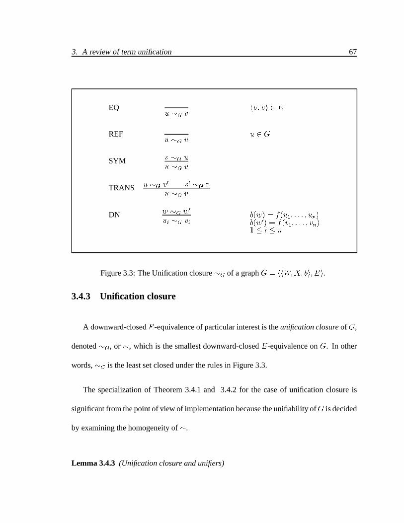
3. A review of term unification 67
EQu �G v
(u; v) 2 E
REFu �G u
u 2 G
SYM v �G uu �G v
TRANS u �G v0 v0 �G vu �G v
DN w �G w0
ui �G vib(w) = f(u1; : : : ; un)b(w0) = f(v1; : : : ; vn)1 � i � n
Figure 3.3: The Unification closure �G of a graph G = hhW;X; bi; Ei.
3.4.3 Unification closure
A downward-closed E-equivalence of particular interest is the unification closure of G,
denoted �G, or �, which is the smallest downward-closed E-equivalence on G. In other
words, �G is the least set closed under the rules in Figure 3.3.
The specialization of Theorem 3.4.1 and 3.4.2 for the case of unification closure is
significant from the point of view of implementation because the unifiability ofG is decided
by examining the homogeneity of �.
Lemma 3.4.3 (Unification closure and unifiers)
3. A review of term unification 68
Let G be a unification graph with a unifier �. Let u; v 2 G. Then u � v implies �(s(u)) =
�(s(v)).
Proof Since � is the smallest downward-closed E-equivalence, it is contained in the
equivalence induced by � on G. a
Corollary 3.4.1 (Unification Closure)
G is unifiable if and only if the unification closure � of G is homogeneous.
Proof If � is homogeneous, then by Theorem 3.4.1, the substitution derived from � is
a unifier. If G is unifiable by some unifier �, then by Lemma 3.4.3, � is contained in the
equivalence R induced by � on G. By Theorem 3.4.2, R is homogeneous. Therefore � is
homogeneous. a
The following example illustrates the unifier derived by the unification closure, and the
homogeneous downward-closed E-equivalence induced by that unifier over a unification
graph:
Example 3.4.9: The set of equivalence classes of the unification closure � of graph G of
Figure 3.2 is
ffz; w1g; ft; w2g; fx; yg; fw3g; fw4gg

3. A review of term unification 69
f
f
g
g
{x, y}
{w3}
{w4}
{t, w2}
{z, w1}
Figure 3.4: Quotient graph G=� of the graph G in Figure 3.2
It is easy to verify that � is homogeneous. The quotient term graph G=�= hW�; X�; b�i
is shown in Figure 3.4, with
W� = ffz; w1g; ft; w2g; fw3g; fw4gg
the set of strict variables X� = ffx; ygg, and b� equal to
fz; w1g = f(fw3g; fz; w1g)
ft; w2g = f(fw4g; fz; w1g)
fw3g = g(fx; yg)
fw4g = g(fx; yg)
Let � be the term defined as � = f(g(fx; yg); �). It is easy to verify that the solution s� of
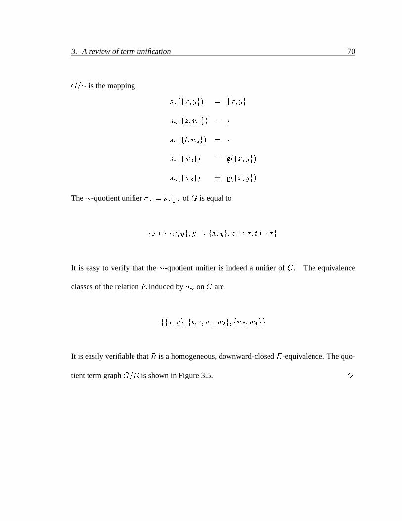
3. A review of term unification 70
G=� is the mapping
s�(fx; yg) = fx; yg
s�(fz; w1g) = �
s�(ft; w2g) = �
s�(fw3g) = g(fx; yg)
s�(fw3g) = g(fx; yg)
The �-quotient unifier �� = s�[]� of G is equal to
fx 7! fx; yg; y 7! fx; yg; z 7! �; t 7! �g
It is easy to verify that the �-quotient unifier is indeed a unifier of G. The equivalence
classes of the relation R induced by �� on G are
ffx; yg; ft; z; w1; w2g; fw3; w4gg
It is easily verifiable that R is a homogeneous, downward-closed E-equivalence. The quo-
tient term graph G=R is shown in Figure 3.5. 3

3. A review of term unification 71
g
f
{x, y}
{w3, w4}
{t, z, w1, w2}
Figure 3.5: Quotient graph G=R of the graph G of Figure 3.2, where R is the equivalenceinduced by the unifier �� on G computed in Example 3.4.9.
3.4.4 Construction of Most General Unifiers
When a unification graph G is non-unifiable, the non-unifiability of G can be traced
to the non-homogeneity of the unification closure � of G. On the other hand, when G is
unifiable, � can be used to construct a most general unifier of G.
Let R be an equivalence relation on the vertices of a unification graph G. A represen-
tative function on R is a function that maps each strict equivalence class of R to a member
of that equivalence class.
Lemma 3.4.4 (Unification closure and most general unifier)
Let G = hW;X; b; Ei be a unification graph, where X � V is the set of strict variables
in G. Let the unification closure of � be homogeneous. Let G=� = hW�; X�; b�i be the
quotient term graph with a solution s�. Let �� = s�[]� be the �-quotient substitution on
G. Let r : X� �! X be a representative function on the strict equivalence classes X� of
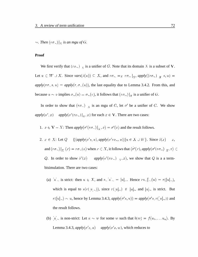
3. A review of term unification 72
�. Then (r��) jX is an mgu of G.
Proof
We first verify that (r��) jX is a unifier of G. Note that its domain X is a subset of V.
Let u 2 W [ X . Since vars(s(u)) � X , and r�� =X r�� jX , apply((r��) jX s; u) =
apply(r��s; u) = apply(r; ��(u)), the last equality due to Lemma 3.4.2. From this, and
because u � v implies ��(u) = ��(v), it follows that (r��) jX is a unifier of G.
In order to show that (r��) jX is an mgu of G, let �0 be a unifier of G. We show
apply(�0; x) = apply(�0(r��) jX ; x) for each x 2 V. There are two cases:
1. x 2 V�X: Then apply(�0(r��) jX ; x) = �0(x) and the result follows.
2. x 2 X: Let Q = fhapply(�0s; u); apply(�0r��; u)iju 2 X [Wg. Since s(x) = x,
and (r��) jX (x) = r��(x)when x 2 X , it follows that h�0(x); apply(�0(r��) jX ; xi 2
Q. In order to show �0(x) = apply(�0(r��) jX ; x), we show that Q is a a term-
bisimulation. There are two cases:
(a) [u]� is strict: then u 2 X , and s�[u]� = [u]�. Hence rs�[]�(u) = r([u]�),
which is equal to s(r([u]�)), since r([u]�) 2 [u]� and [u]� is strict. But
r([u]�) � u, hence by Lemma 3.4.3, apply(�0s; u)) = apply(�0s; r([u]�)) and
the result follows.
(b) [u]� is non-strict: Let u � w for some w such that b(w) = f(u1; : : : un). By
Lemma 3.4.3, apply(�0s; u) = apply(�0s; w), which reduces to
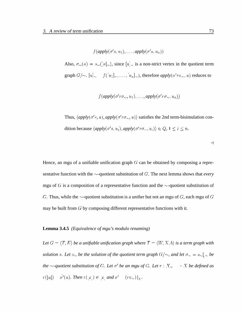
3. A review of term unification 73
f(apply(�0s; u1); : : : ; apply(�0s; un))
Also, ��(u) = s�([u]�), since [u]� is a non-strict vertex in the quotient term
graph G=�. [u]� = f([u1]�; : : : ; [un]�), therefore apply(�0r��; u) reduces to
f(apply(�0r��; u1); : : : ; apply(�0r��; un))
Thus, happly(�0s; u); apply(�0r��; u)i satisfies the 2nd term-bisimulation con-
dition because happly(�0s; ui); apply(�0r��; ui)i 2 Q, 1 � i � n.
a
Hence, an mgu of a unifiable unification graph G can be obtained by composing a repre-
sentative function with the �-quotient substitution of G. The next lemma shows that every
mgu of G is a composition of a representative function and the �-quotient substitution of
G. Thus, while the �-quotient substitution is a unifier but not an mgu of G, each mgu of G
may be built from G by composing different representative functions with it.
Lemma 3.4.5 (Equivalence of mgu’s modulo renaming)
Let G = hT;Ei be a unifiable unification graph where T = hW;X; bi is a term graph with
solution s. Let s� be the solution of the quotient term graph G=�, and let �� = s�[]� be
the �-quotient substitution of G. Let �0 be an mgu of G. Let r : X� �! X be defined as
r([u]) = �0(u). Then r([x]) 2 [x] and �0 = (r��) jX .

3. A review of term unification 74
Proof It is easy to verify that r is a representative function for �. By Lemma 3.4.4,
(r��) jX is an mgu of G. Since the domain of (r��) jX is X , it follows that dom(�0) � X .
We verify that apply(�0; u) = apply((r��) jX ; u) for each x 2 V. There are two cases:
1. u 2 V�X: both �0(u) and apply((r��) jX ; u) reduce to u.
2. u 2 X: Let Q = fhapply(�0s; u); apply(r��; u)iju 2 X [Wg. Since s(u) = u, and
�� jX (u) = �(u) when u 2 X , fhapply(�0; u); apply(r��; u)iju 2 Xg � Q. It is
easy to verify that Q is a is a term-bisimulation.
a
Thus, an mgu of a unifiable unification graph is unique modulo renaming, with the under-
standing that the renaming refers to the renaming substitution from the representatives of
strict equivalence classes used in one mgu to those of the other mgu. This is illustrated in
the next example.
Example 3.4.10: Let E = fu?= f(x; y); y
?= z; x
?= vg be a system of equations whose uni-
fication graph isG = hW;X; b; EiwhereW = fwg,X = fx; y; z; u; vg, b = fw = f(x; y)g,
and E = f(u; w); (y; z); (x; v)g. Then the set of equivalence classes of the unification
closure � of G is ffw; ug; fx; vg; fy; zgg. The quotient graph is hW�; X�; b�i, where
W� = fw; ug, X� = ffx; vg; fy; zgg. The �-quotient unifier �� is
�� = fx 7! fx; vg; v 7! fx; vg; y 7! fy; zg; z 7! fy; zg; u 7! f(fx; vg; fy; zg)g

3. A review of term unification 75
Let r1; r2 : X� �! X be two representative functions, and let �1 = (r1��) jX , and
�2 = (r2��) jX be two mgu’s:
r1 = ffx; vg 7! x; fy; zg 7! yg
r2 = ffx; vg 7! v; fy; zg 7! zg
�1 = fx 7! x; v 7! x; y 7! y; z 7! y; u 7! f(x; y)g
�2 = fx 7! v; v 7! v; y 7! z; z 7! z; u 7! f(v; z)g
Here ind(�1) = fx; yg, and ind(�2) = fv; zg. Note that ri([u]) = �i(u); u 2 X , for
i 2 f1; 2g. The renaming function �12 = fx 7! v; y 7! zg maps the range of r1 to the
range of r2, and the renaming function �21 = fx 7! v; y 7! zg maps the range of r2 to the
range of r1. �12 and �21 are inverses of each other, and �2 = �12�1, and �1 = �21�2. This
shows that �1 and �2 are equal modulo renaming. 3
If E is a system of equations with mgu s, the set of independent variables of E under s
is defined as ft 2 vars(E) j s(t) = tg. It is clear that if s is an mgu of a system of equations
E, s(t) = t for all variables t 62 vars(E). For this reason, we may assume that if s is an
mgu of E, vars(s) � vars(E).
3. A review of term unification 76
3.5 The unification algorithm
This section presents a simple implementation of the unification algorithm for well-
founded terms. The algorithm takes a pair of pointed term graphs which are directed acyclic
graphs, and determines if the terms represented by them are unifiable.
The first formal account of the term unification problem and the discovery of the uni-
fication algorithm is generally credited to J. A. Robinson [91]. The original algorithm
by Robinson, based on a representation of terms by means of linear sequence of sym-
bols was exponential in time and space complexity. The space complexity was later im-
proved by using a tabular data structure Robinson [92]. The idea of representing terms as
graphs with structure sharing, proposed by Boyer and Moore [11], greatly improved the ef-
ficiency of representing terms. Algorithms with quadratic time complexity were proposed
by Venturini-Zilli [105], and Corbin and Bidoit [23]. Almost linear time algorithms were
proposed by G. Huet [51], L.D. Baxter [7]). Finally, linear time unification algorithms were
proposed by Paterson and Wegman [84] and Martelli and Montanari [67].
The unification algorithm is presented as the procedure unify and three auxiliary proce-
dures union, find and occurs? shown in Figures 3.6 through 3.8.
The unification graph is represented as a data structure consisting of a set of variables
(vertices) linked together by pointers. Each variable has a type, which is either strict or
functor. Each functor variable v has a field v:L denoting the functor label of v. If the arity

3. A review of term unification 77
1 procedure unify(v1; v2) =2 let r1 = find(v1) and r2 = find(v2)3 in if r1 = r2 then return4 else case r1:type; r2:type5 strict, strict: union(r1; r2)6 functor, strict: unify(v2; v1)7 strict, functor: let ans = occurs?(r2; r1)8 in case ans9 no: union(r1; r2)10 yes: fail(CYCLE)11 functor,functor:12 if r1:L 6= r2:L then fail(CLASH)13 else14 union(r1; r2);15 for i = 1 to arity(r1:L) do16 unify(r1:child(i); r2:child(i))
Figure 3.6: Unification algorithm: procedure unify
17 procedure union(r1; r2) = r1:binding := r2
18 procedure find(v) =19 if unbound?(v) then return v20 else let v0 = v:binding21 in let r = find(v0) in return r
Figure 3.7: Unification algorithm: procedures union and find
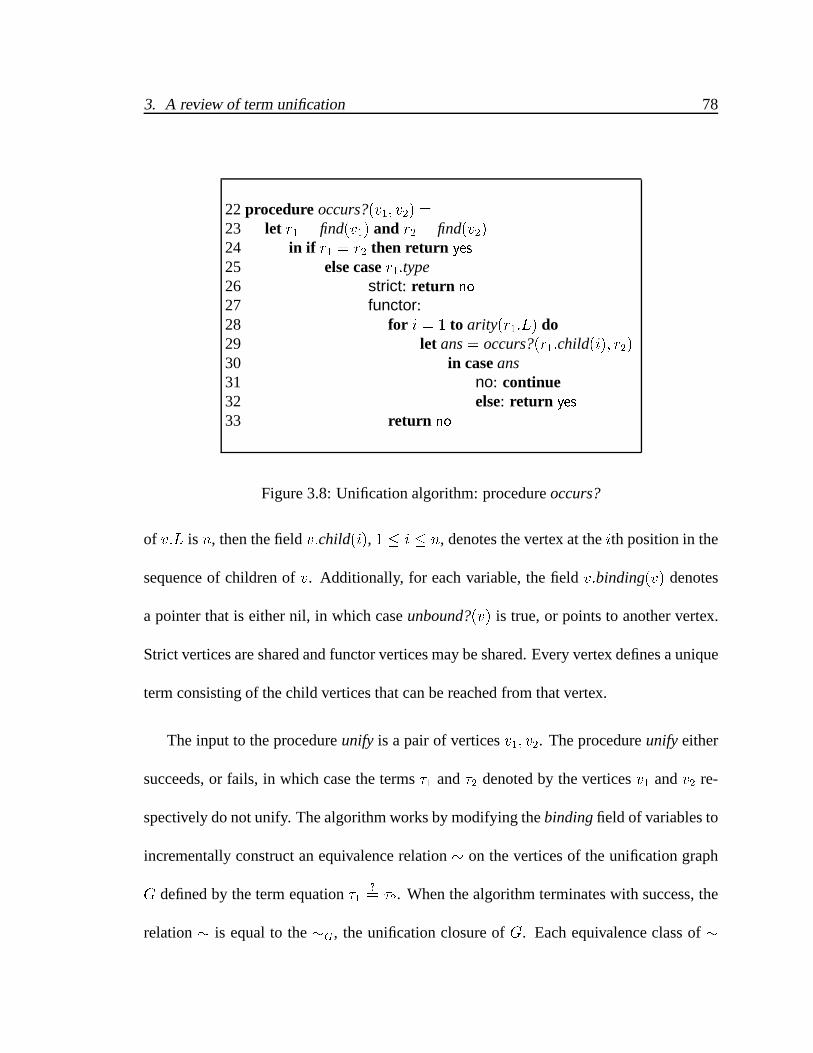
3. A review of term unification 78
22 procedure occurs?(v1; v2) =23 let r1 = find(v1) and r2 = find(v2)24 in if r1 = r2 then return yes
25 else case r1:type26 strict: return no
27 functor:28 for i = 1 to arity(r1:L) do29 let ans = occurs?(r1:child(i); r2)30 in case ans31 no: continue32 else: return yes
33 return no
Figure 3.8: Unification algorithm: procedure occurs?
of v:L is n, then the field v:child(i), 1 � i � n, denotes the vertex at the ith position in the
sequence of children of v. Additionally, for each variable, the field v:binding(v) denotes
a pointer that is either nil, in which case unbound?(v) is true, or points to another vertex.
Strict vertices are shared and functor vertices may be shared. Every vertex defines a unique
term consisting of the child vertices that can be reached from that vertex.
The input to the procedure unify is a pair of vertices v1; v2. The procedure unify either
succeeds, or fails, in which case the terms �1 and �2 denoted by the vertices v1 and v2 re-
spectively do not unify. The algorithm works by modifying the binding field of variables to
incrementally construct an equivalence relation � on the vertices of the unification graph
G defined by the term equation �1?= �2. When the algorithm terminates with success, the
relation � is equal to the �G, the unification closure of G. Each equivalence class of �
3. A review of term unification 79
is maintained as a tree of vertices linked by the binding pointer whose root is representa-
tive vertex of the equivalence class. The binding pointer is manipulated by the following
auxiliary procedures:
1. The procedure find(v) iteratively follows the binding pointer and returns the repre-
sentative vertex of the equivalence class of� containing v. The binding pointer of the
representative vertex is assumed to be nil. The representative of a non-strict equiva-
lence class (one containing at least one functor vertex) is always a functor vertex.
2. The procedure union(u; v) sets the binding pointer of u to be equal to v, where u
and v are representative of different equivalence classes, thereby merging the two
equivalence classes into one whose representative is v.
3. The procedure occurs?(u; v) returns yes or no depending on whether the term de-
noted by the equivalence class containing v is a subterm of the term denoted by the
equivalence class containing u in the quotient graph G=�.
The occurs? predicate is also known as the occurs check and is used by the unify pro-
cedure to determine if the unification closure is cyclic. In the “standard” version of the
unification algorithm, which is shown in Figure 3.6 and which computes acyclic mgu’s of
term equations consisting of wellfounded terms, unify fails with CYCLE if the occurs check
returns a yes. For unification of rational terms, where the terms or the unification closure
may be cyclic, the occurs check can simply be omitted from the unify procedure. Often,
3. A review of term unification 80
unification algorithms omit the occurs check from the unify procedure and perform the test
in a separate phase.
The call unify(v1; v2) first computes the representatives r1 and r2 of the equivalence
classes containing the vertices v1 and v2 respectively (line 2). If the representatives are
identical, then u and v are already unified, and there is nothing to do. If the two are distinct,
then if both equivalence classes are strict, then the two are merged (line 5). Line 6 reverses
the arguments in order to ensure that the representative r2 of the merged equivalence class
is a functor variable if the merged equivalence class is non-strict. Line 7 tests if the term
denoted by r1 occurs in the term denoted by r2 in the quotient graph G=�. If the occurs-
check is false, the equivalence classes are merged (line 9), otherwise the procedure unify
fails, indicating that the unification closure is cyclic. If both representatives are functor
nodes (line 11), and their labels do not match, unify fails signaling a CLASH (line 12).
Otherwise, the two equivalence classes are merged (line 14) and the the corresponding
children of the two functor nodes are unified (lines 15, 16).
The algorithm presented here operates on term graphs and uses linear space but expo-
nential time in size of its input. However, this naıve implementation lends itself to ease of
exposition, and later on, to easy modification. The source of exponential behavior is the
occurs-check function. With better data structures, however, occurs-check can be easily im-
plementated in linear time, bringing the complexity of the algorithm down to quadratic. By
moving the occurs-check “offline,”, that is, out of unify, and implementing find and union
3. A review of term unification 81
using a technique called path compression, based on Tarjan’s union-find algorithm [99], the
complexity of the algorithm can be brought down to almost linear time. Finally using Pa-
terson and Wegman’s algorithm [84], the complexity of unification for wellfounded terms
can be brought down to linear time.
The unification algorithm maintains the following invariants:
Lemma 3.5.1 (Unification invariants)
Let G be a unification graph of a term equation �1?= �2 between the terms �1 and �2
represented by the term graphs rooted at vertices v1 and v2. Let the unification closure of
G be denoted�. Then the following invariants are maintained by the unification algorithm:
1. For each call unify(u; v), G j= u � v.
2. For each call union(r1; r2), G j= r1 � r2.
3. If find(v) = r, then G j= v � r.
4. If occurs?(u; v) = yes, then G=�j= [u]���! [v]�.
Proof (Sketch)
The invariant (1) is true for the “top-level” call. For subsequent calls, the invariant
is true because of the equivalence and downward-closure of �. Similarly, for each call to
union(r1; r2) inside a call to unify(v1; v2), r1 = find(v1) and find(r2) = v2. By the induction

3. A review of term unification 82
hypothesis, r1 � v1 and r2 � v2 and v1 � v2. Hence the result follows. To show (3) the
call is true the first time when unbound?(v) is true. For each subsequent call, the result is
true by transitivity. The proof of (4) follows from (3) and the inductive hypothesis, when
find(u) 6= find(v). a
Non-unifiability is characterized by the following special case:
Corollary 3.5.1 Let G be a unification graph of a term equation �1?= �2 between the terms
�1 and �2 represented by the term graphs rooted at vertices v1 and v2. Let the unification
closure of G be denoted �. Then
1. If unify(v1; v2) = fail(CY CLE), then G=�j= [u]+�! [u] for some u 2 G.
2. If unify = fail(CLASH), then G=�j= [w] = [w0] for some w;w0 such that L(w) 6=
L(w0).
The above result captures the conditions for non-unifiability of a unification graph in
terms of properties of the quotient of the unification graph. The operational details of
deriving such a condition for non-unifiability is the theme of the next chapter.
3.6 Summary
This chapter formalized the problem of unification of rational terms. Rational terms
were defined as co-inductive objects, and extensionality was defined via term-bisimulations.

3. A review of term unification 83
The notion of unification of a system of term equations, unifiers, and most general unifier
were defined. Unifiability reduces to computing the homogeneity of the unification closure
of a unification graph. A simple unification algorithm that determines the unifiability of a
pair of term equations was presented.
4
Path expression logics for unifiability
The last chapter showed how the unifiability of a system of equations is determined by
the homogeneity and acyclicity of the quotient graph G=� of the graph G representing
the term equations. However, it left open the question of source-tracking: how to express
unifiability directly in terms of connectivity relation on the source graph G, rather than the
quotient graph.
This chapter uses the logic of path deductions for expressing connectivity relations on
a labeled directed graph. Using the “formulas as types and proofs as programs” notion,
also known as the Curry-Howard isomorphism (Howard [49]), paths can be viewed as en-
coding proofs of connectivity in a graph. Using this interpretation, the type of a path is
its endpoints. The set of paths is thus a typed subset of the elements of the algebra of the
untyped free monoid generated by the edges of a directed labeled graph. Each path also
has an associated semantics, which is the label of the path. Source-tracking of unification
84

4. Path expression logics for unifiability 85
is based on considering bidirectional paths over a labeled directed graphs G: that is paths
in the graph G [ G�1, where G�1 is obtained by reversing the direction of edges in G. In
other words, edges can be traversed either positively (from source to destination) or neg-
atively, from destination to source. Unification closure may be viewed as a connectivity
relation by interpreting the downward-closure rule as building a bidirectional path connect-
ing vertices through their parents. Source-tracking unification involves computing paths
witnessing connectivity in a labeled directed graph G, where positive and negative traver-
sal is permitted, and relating them to paths witnessing connectivity in the quotient graph
G=�, where only positive traversal is permitted.
Connectivity in the original graph does not guarantee connectivity in the quotient graph.
That is determined by properties of the label semantics of the path witnessing the connec-
tivity in original graph. Roughly speaking, an empty path in the quotient graph corresponds
to a path in the original graph whose positive and negative traversals cancel out, while a
non-empty path in the quotient graph corresponds to a path in the original graph that is
left with a net positive traversal. The subset of paths in the original graph that can be thus
related to paths in the quotient graph are called unification paths. If the labels on branch
edges and their inverses are interpreted as closed and open parentheses, respectively, then
the labels of unification paths are sentences in the context-free language of balanced paren-
theses (the semi-Dyck languages) and their suffixes.
Various classes of paths are expressed as “well-typed terms” drawn from a free algebra
4. Path expression logics for unifiability 86
of terms over the edges of a labeled directed graph. The logic �, introduced in Section 4.2,
computes paths in a directed labeled graph. �2, computes bidirectional paths, while �U
computes unification paths. In the logic PU , path terms are drawn from the term algebra
whose signature is that of a group. Unification path expressions may be simplified (nor-
malized) to unification paths.
The logics PU and �U may be viewed as an operational semantics of unification. The
construction of PU deductions is easily integrated into the unification algorithm with the
addition of a proof parameter. The unification algorithm maintains the invariant that at each
call of unify(u; v; p), p is the proof of the membership of the pair (u; v) in the unification
closure over a graph G containing vertices u and v. The construction of these proofs incurs
only a constant overhead per unification call.
The path expression logicsPU and�U are equivalent to the logic LE0 of Le Chenadec [64].
The systems �U , PU and LE0 are all sound and complete with respect to the connectivity
in the quotient graph. However, PU and �U are logics about connectivity between vertices
in a graph, rather than equality between terms. They make the connection with formal lan-
guage path problems more explicit and suggest a more direct route to implementation with
existing unification algorithms.
An important measure of the quality of source-tracking information is the absence of
irrelevant details in that information. Simplification of source-tracking information is im-
plemented by a convergent rewrite system operating on path expressions and paths. Subject

4. Path expression logics for unifiability 87
reduction guarantees that simplification preserves the endpoint type and label semantics of
the path.
Section 4.1 reviews the basic results about � algebras and Semi-Dyck sets, the basis
for encoding unification proofs. Section 4.2 introduces the logics � and �2. Section 4.3
presents the logic �U for unification paths. Section 4.4 introduces the logic PU of uni-
fication path expressions. Section 4.5 shows how the computation of PU proofs can be
integrated into the unification algorithm.
4.1 Preliminaries
4.1.1 �-Algebras
In this section, we recapitulate basic results of the algebraic theory of data types: �-
algebras, homomorphisms, initial, free and quotient algebras. The notation used here has
been (partly) borrowed from (Baader and Nipkow [2]).
Given a signature �, a �-algebra A is a pair hA; ai, where A is a set, and a : �(A) �!
A is a function from �(A) to A. The set A is called the carrier ofA. Thus, for each f 2 �,
if arity(f) = n, a(f(a1; : : : ; an)) is an element ofA. We can also think of a(f) as a function
from An to A. a(f) is then called the interpretation of f in A. Much of the discussion in
the rest of the chapter relies on the monoid signature �Mon = f(�; 0); (�; 2)g, and group

4. Path expression logics for unifiability 88
signature �Gr = �Mon [ f(:)�1; 1)g.
Let � be a signature. If h : A �! B is a function, then �(h) : �(A) �! �(B) denotes
the function that maps each element f(a1; : : : ; an) of�(A) to the element f(h(a1); : : : ; h(an)).
Given �-algebras A = hA; ai and B = hB; bi, a function h : A �! B is a homomorphism
from A to B if ha = b�(h). If � is a signature and V is a set of variables, T (�; V ), the
�-term algebra generated by V is the �-algebra whose carrier is T �(�; V ), and for each
f 2 � of arity n, a(f; t1; : : : ; tn) = f(t1; : : : ; tn). �-term algebras are important because
if T (�; V ) is a �-term algebra and B = hB; bi is any �-algebra, then for each function
h : V �! B, there is a unique homomorphism from T (�; V ) to B, called the homomor-
phic extension of h. The homomorphic extension of h is often indicated by h itself, but
sometimes it is denoted h in order to distinguish it from h.
IfA = hA; ai is a �-algebra, an equivalence relationR onA is a congruence, if for each
f 2 � such that arity(f) = n, and for each ai R a0i, 1 � i � n, f(a1 : : : ; an)R f(a01 : : : ; a0
n).
The quotient algebra A=R is the �-algebra hA=R; a=Riwhose carrier set A=R is the set of
equivalence classes [u]R = fv 2 A j u R vg of R, and for each f 2 � with arity(f) =
n, and for each [ai] 2 A=R, 1 � i � n, a=R(f([a1]R; : : : ; [an]R)) is defined to be
[a(f(a1; : : : ; an))]R.
Given a signature � and a denumerable set V of variables, a �-identity is a pair s � t,
where s; t are elements of T �(�; V ). The set of�-identities of interest in this chapter are the
monoid identities Mon = fp � (q � r) � (p � q) � r; � � p � p; p � � � pg, and the group
4. Path expression logics for unifiability 89
identities Gr = fp � (q � r) �; (p � q) � r; p�1 � p � �; p � � � pg. A �-identity s � t
holds in a �-algebra A, written A j= s � t, if for every homomorphism h : T (�; V ) �!
A, h(s) = h(t). A �-algebra A is a model for a set of �-identities E, written A j= E,
if for each s � t 2 E, A j= s � t. A monoid is a �Mon-algebra that models the set of
identities Mon. A group is a �Gr-algebra that models the set of identities Gr. A pair
s � t is a semantic consequence of E, written E j= s � t, if for each A such that A j= E,
A j= s � t. The set of all semantic consequences of E is called the equational theory of
E and is denoted �E . By Birkhoff’s theorem, �E is equal to the least equivalence relation
over T �(�; V ) containing E that is closed under substitutions and congruences.
If X is a set, then T (�Mon; X)= �Mon, abbreviatedMon(X), is called the free monoid
generated byX . It is easy to verify thatMon(X) is a monoid. Similarly, T (�Gr; X)= �Gr,
abbreviated Gr(X), is the free group generated by X . It is easy to see that the carrier of
Mon(X) is isomorphic to the set X� of sentences over X .
4.1.2 Semi-Dyck and Dyck languages
The class of languages identified by balanced parentheses, known as the Semi-Dyck
sets, are important from both practical and theoretical standpoint in computer science. Be-
cause of its uniformity and ease of parsing, notation based on nested, balanced parentheses
has proved ideal for representing textual data and also programs.
4. Path expression logics for unifiability 90
Semi-Dyck sets also play an important role in the theory of formal languages, where
they are known to characterize the full class of context-free languages [19] from which the
class of recursively enumerable sets may be characterized (see for example, Savitch [94]).
The main result of this chapter is concerned with showing how unification proofs can be
encoded as paths whose labels are sentences of a Semi-Dyck set. In this section, we briefly
review the definitions of Semi-Dyck and Dyck sets and related languages. We discuss their
grammars, cancellative properties, and their connection with groups. Semi-Dyck and Dyck
languages are treated in detail by Harrison [42].
Let � = fb1; : : : ; bng be an alphabet. Then the alphabet ��1 = fb�1i j bi 2 �g, as-
sumed disjoint from �, consists of matching symbols such that for each bi 2 �, there is
a unique matching symbol b�1i 2 ��1. The symbols in � are called closed �-parenthesis
symbols, and those in ��1 are called open �-parenthesis symbols. D(�) denotes the set
fb�1b � � jb 2 �g consisting of one-way cancellative identities. D0(�) denotes the set
fbb�1 � �; b�1b � �; b 2 �g consisting of left and right cancellative identities. When � is
clear from the context, we abbreviate these sets of identities as D andD0, respectively. Let
�D and �D0 denote the smallest congruences over (� [ ��1)� containing the identities D
and D0, respectively. Intuitively, u �D v if u may be obtained from v via applications of
the identities in D (or vice versa), and likewise for u �D0 v. The equational systems D
and D0 may be turned into rewrite systems by orienting each of the identities b�1b � �
and bb�1 � � as b�1b �! � and bb�1 �! �, respectively. Thus, the rewrite system D(�)

4. Path expression logics for unifiability 91
consists of the rules
fb�1b �! � j b 2 �g
and the rewrite system D0(�) is equal to D(�) [ fbb�1 �! � j b 2 �g. It is easy to show
that the rewrite systemsD andD0 are convergent (terminating and confluent) and complete
with respect to the corresponding equational systems D and D0. We denote by �D(�)(x)
and �D0(�)(x), the (unique) normal forms underD(�) andD0(�) rewriting, respectively, of
a sentence x 2 (�[��1)�. For example, if � = f]g, and ��1 = f[g, then �D(�)(][) =][, but
�D0(�)(][) = �. The normal form of a sentence p may be computed in a single left-to-right
pass of p in time O(jpj).
Given L � (� [ ��1)�, let
D(�; L)def= fl 2 (� [ ��1)� j �(l) 2 Lg
D0(�; L)def= fl 2 (� [ ��1)� j �0(l) 2 Lg
We are primarily interested in the languages D(�; L), when L is �0 = f�g, �+, or
��. These are abbreviated D0(�), D+(�), and D�(�), respectively. When � is clear from
context, these are further abbreviated to D0, D� and D+. The language D0(�) is known
as the semi-Dyck set over �, and the language D0(�;�0), abbreviated D00 is known as the
Dyck set over �.
D0 and D+ are mutually disjoint, and D� = D0 [D+. It can be seen that D� is the set
4. Path expression logics for unifiability 92
of all suffixes of D0 sentences, and is suffix-closed. (See Harrison [42], page 314, for the
symmetric case of prefixes of D0 sentences.) Thus D+ may be informally characterized as
the set of “unbalanced” suffixes of sentences of balanced parentheses. The languages D0,
D+, and D� are generated using the following context-free grammar:
D0 ::= � jD0b�1D0bD0 b 2 �
D+ ::= D�bD� b 2 �
D� ::= D0 j D+
Example 4.1.11: If � = f); ]g and ��1 = f(; [g, then the set of D(�) consists of the
identities ( ) = � and [ ] = �. The sentences ‘([ ])’, and ‘(( )[ ])’ are in D0. ‘( ) [ ] ]’, ‘( ) ]’
are in D+ and they are both reduce to ] by the rewrite system D(�). The sentence ‘( ] )’ is
not in D�. 3
The next lemma formalizes the intuition that for every D� sentence l, every open paren-
thesis occurring in l is matched, and every closed parenthesis is either matched, or un-
matched. In the latter case, l is in D+.
Lemma 4.1.1 (Decomposition)
Let � be an alphabet. If l 2 D�(�), then
1. If l = p��1q for some � 2 �, then q = x�y, where x 2 D0

4. Path expression logics for unifiability 93
2. If l = p�q, for some � 2 �, then
(a) p = x��1y, where y 2 D0, or
(b) p; q 2 D�, implying l 2 D+
Proof By induction on the derivation of D� sentences. a
We now consider another example of using cancellative identities to reduce D� sen-
tences.
Example 4.1.12: Consider the sentence l equal to (1)2(3)4 consisting of left and right
parentheses symbols indexed for identification. If � = f(g, and ��1 = f)g, then l is in
D0(�). l can be reduced to � using the one-sided cancellative rule () �! � with (1 and )2
cancelling each other, and similarly (3 and )4. However, l may be reduced to � using two-
sided cancellative rules f() �! �; )(�! �g as well: )2 and (3 cancel each other, leaving the
sentence (1)4 which reduces to � using the rule () �! �. 3
The above example hints that D�-sentences are closed under two-sided cancellation.
This means that when reducing D�-sentences, two-sided cancellative identities may be
employed, rather than one-sided cancellative identities.
Lemma 4.1.2 (Subject reduction of D�-sentences under D0 rewriting)
Let � be an alphabet. If l 2 D�(�) and l �!D0 l0, then l �D l0.

4. Path expression logics for unifiability 94
Proof By a case analysis on the rules of D0. Let � 2 �.
1. ��1� �! �: l = r��1�s and l0 = rs for some r; s 2 (� [ ��1)�. Since the redex
��1� is being reduced to �, and ��1� � � 2 D(�), it follows that l �D(�) l0.
2. ���1 �! �: l = r���1s and l0 = rs, for some � 2 � and r; s 2 (� [ ��1)�. By
Lemma 4.1.1, s = s1�s2, where s1 2 D0. Again, since � occurs in l, there are two
cases:
(a) r = r1��1r2, where r2 2 D0: Therefore,
l = r���1s Given
= r1��1r2��
�1s1�s2 Lemma 4.1.1
��!D r1��s2 Since r2; s1 2 D0
��!D r1s2 and
l0 = rs Given
= r1��1r2s1�s2 Since r = r1�
�1r2, s = s1�s2
��!D r1�s2 Since r2; s1 2 D0
��!D r1s2
Hence, we have, l �D(�) r1s2 �D(�) l0,
(b) r 2 D�(�) and �s 2 D�. Therefore, l = r���1s1�s2. Since s1 2 D0, l ��!D
r�s2. Also, l0 = rs1�s2. Since s1 2 D0, l0 ��!D r�s2. Hence both l and l0
4. Path expression logics for unifiability 95
reduce to r�s2, implying l �D(�) r�s2 �D l0.
a
Dyck sets are closely related to groups. The quotient monoid (� [ ��1)�= �D0� has
D00(�) as its identity element. By defining a unary inverse operation [w]�1 = [w0], where
ww0 �D0(�) �, the quotient monoid can be made into a group. This group is isomorphic to
the free group generated by �. The isomorphism f maps each class [w] of �D0 containing
w to the class of the free group containing w with the property that [w] � f([w]).
It is natural to define an inverse operation inv directly on sentences as follows: inv(�) =
�, inv(c) = c�1, for c 2 �, inv(c�1) = c, for c 2 ��1, and for each p; q that are sentences
over � [ ��1, inv(pq) = inv(q)inv(p). The free monoid (� [ ��1)�, along with inv, is a
�Gr-algebra. The inverse operation can be modeled by two-sided cancellation: q = inv(p)
implies qp �D0 �.
4.1.3 �-graph representation of unification graphs
In the last chapter, we assumed unification graphs were represented by a union of term
graphs and undirected equational edges. In order to represent a unification graph as a �-
graph, we simply orient each equational edge in an arbitrary direction and assign the label
� to it. Formally, a �-term unification graph G = hX;W; b; Ei is represented as a �-graph
hV; L;Di in which V = X [ W , L(x) = ; if x 2 X , and L(w) = fhd(b(w))g, and
4. Path expression logics for unifiability 96
D = fwf:i�! v j f 2 L(w) and b(w)(i) = ug [ fu
��! v j (u; v) 2 Eg. Therefore, the �-
graph hV; L;Di ofG is constructed by augmenting the �-term graph hX;W; biwith a set of
directed equational edges: for each pair of vertices in (u; v) 2 E, there is an edge u ��! v.
The notation c : u��! v 2 D is shorthand used for the statement “the edge u
��! v,
abbreviated c, is in D.”
Thus, labeled directed graphs generalize both term graphs and unification graphs. Unifi-
cation closure can be defined directly on labeled directed graphs. LetG = h�V ;�D; V; L;Di
be a labeled directed graph. The set of �-edges of G is the set f(u; v) 2 D j u�
�! v 2 Dg.
The unification closure of a labeled directed graph is the smallest downward-closed equiv-
alence relation on the vertices V containing the �-edges of G.
Example 4.1.13: The unification graph of Example 3.4.7 is represented by the �-graph
G = hV; L;Di, where � = hf 7! 2; g 7! 1i. The graph is shown in Figure 4.1. The
equational edges a1, a2 and a3 are labeled �. The branch edges b1 and b4 are labeled f:1,
while the branch edges b3 and b6 are labeled f:2. The branch edges are b2 and b5 are labeled
g:1. 3
Directed equational edges are distinguished by thin, transparent arrowheads and are
implicitly labeled �, while branch edges are identified with thicker, solid arrowheads.

4. Path expression logics for unifiability 97
f
f
gw2
w3
w4g
yx
w1
z
a1
a2
a3
b1
b2
b3
b4
b5
b6t
Figure 4.1: Unification graph G of Example 3.4.7 represented as a directed, labeled graph
4. Path expression logics for unifiability 98
4.2 Path Logics
In this section, we identify various types of connectivity relations on the vertices of
labeled directed graphs. These relations are expressed as a “type system” of path terms. The
first of these logics, called �, identifies labeled paths over a directed graph G. The second,
�2, identifies bidirectional paths over a directed graph, which are paths over G [ G�1,
where G�1, the inverse of G is obtained by reversing the orientation of the edges of G. The
third, �U , identifies unification paths, which are labeled paths over G that encode proofs
of membership in the unification closure of a unification graph.
4.2.1 Paths over labeled directed graphs
Let G = h�V ;�D; V; L;Di be a labeled directed graph. The set of labeled paths in
G may be identified as those sentences over D obtained from deductions in the logic of
a type system �(G) shown in Figure 4.2. The rules of � are directly derived from the
inductive definition of a path. Judgements in �(G) are of the form ` p : ul
�! v. Here,
G is a labeled directed graph, p is a sentence over D, u and v are vertices in G, and l is a
sentence over �D. We write `�(G) p : ul
�! v to denote that there is a deduction D in the
logic � whose final step is the judgement p : u l�! v. The logic � is sound and complete
with respect to labeled paths in a labeled directed graph:
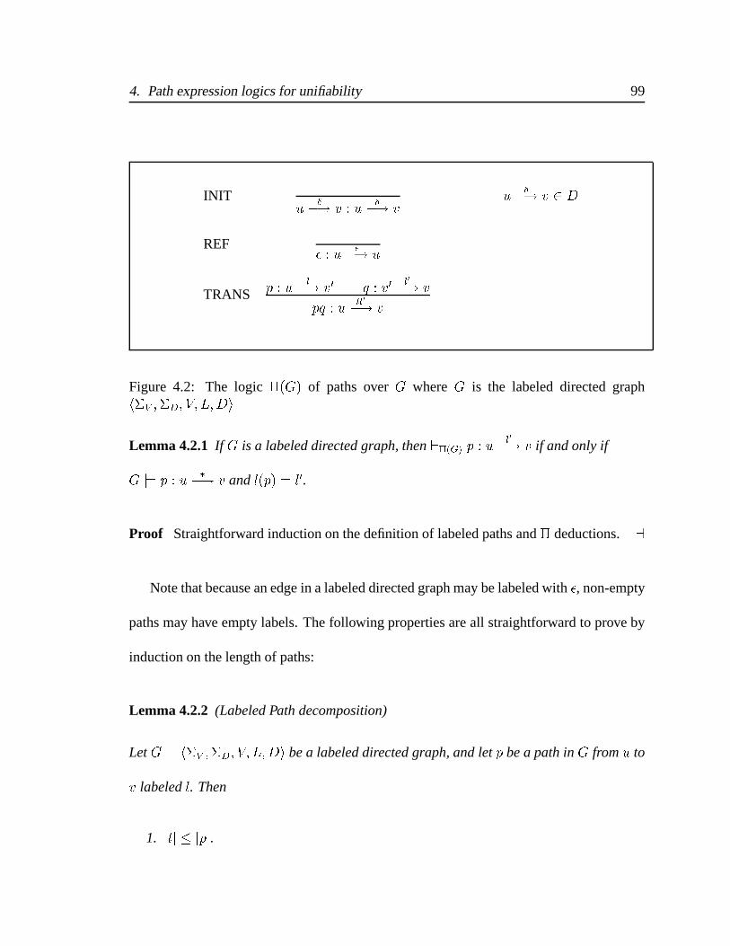
4. Path expression logics for unifiability 99
INITu
��! v : u
��! v
u��! v 2 D
REF� : u
��! u
TRANS p : ul
�! v0 q : v0l0�! v
pq : ull0�! v
Figure 4.2: The logic �(G) of paths over G where G is the labeled directed graphh�V ;�D; V; L;Di
Lemma 4.2.1 If G is a labeled directed graph, then `�(G) p : ul0�! v if and only if
G j= p : u��! v and l(p) = l0.
Proof Straightforward induction on the definition of labeled paths and � deductions. a
Note that because an edge in a labeled directed graph may be labeled with �, non-empty
paths may have empty labels. The following properties are all straightforward to prove by
induction on the length of paths:
Lemma 4.2.2 (Labeled Path decomposition)
Let G = h�V ;�D; V; L;Di be a labeled directed graph, and let p be a path in G from u to
v labeled l. Then
1. jlj � jpj.
4. Path expression logics for unifiability 100
2. If l1l2 = l, there is a vertex v0 paths q and r in G, such that G j= q : u��! v0,
l(q) = l1, G j= r : v0��! v, l(r) = l2 and p = qr.
3. If l = x�y, where � 2 �D, then there are vertices u0 and v0 in V and an edge c
from u0 to v0 labeled �, and paths q and r such that G j= q : u��! u0, l(q) = x,
G j= r : v0��! v, l(q) = y, and p = qcr.
Proof By induction on p. a
4.2.2 Bidirectional Paths
Let G = h�V ;�D; V; L;Di be a labeled directed graph. The inverse of G, G�1, is the
labeled directed graph h�V ;��1D ; V; L;D�1i, where D�1 = fv
��1
�! u j u��! v 2 Dg. We
define ��1 = �. Thus, G�1 is obtained from G by reversing the direction of each edge in
G, changing each edge label � to ��1, and leaving the label � unchanged. G [ G�1 is the
labeled directed graph h�V ;�D [ ��1D ; L; V;D [D�1i. The set of bidirectional labeled
paths over G is the set of labeled paths over G [ G�1. The set of bidirectional paths are
identified by the deductions in the logic �2 of Figure 4.3.
It is easy to see that if G = h�V ;�D; V; L;Di is a labeled directed graph, then p is a
bidirectional path in G from u to v if and only if inv(p) is a bidirectional path in G from v
to u. Furthermore l(inv(p)) = inv(l(p)).
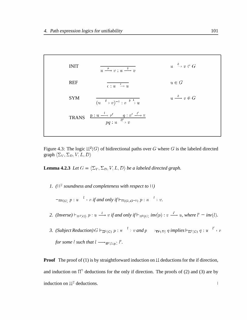
4. Path expression logics for unifiability 101
INITu
��! v : u
��! v
u��! v 2 G
REF� : u
��! u
u 2 G
SYM(u
��! v)�1 : v
��1
�! uu
��! v 2 G
TRANS p : ul
�! v0 q : v0l0�! v
pq : ull0�! v
Figure 4.3: The logic �2(G) of bidirectional paths over G where G is the labeled directedgraph h�V ;�D; V; L;Di
Lemma 4.2.3 Let G = h�V ;�D; V; L;Di be a labeled directed graph.
1. (�2 soundness and completeness with respect to �)
`�2(G) p : ul
�! v if and only if `�(G[G�1) p : ul
�! v.
2. (Inverse) `�2(G) p : ul
�! v if and only if `�2(G) inv(p) : v l0�! u, where l0 = inv(l).
3. (Subject Reduction)G `�2(G) p : ul
�! v and p �!D0(D) q implies`�2(G) q : ul0�! v
for some l such that l �!D0(�D) l0.
Proof The proof of (1) is by straightforward induction on � deductions for the if direction,
and induction on �2 deductions for the only if direction. The proofs of (2) and (3) are by
induction on �2 deductions. a
4. Path expression logics for unifiability 102
Among the set of bidirectional paths over a labeled directed graph, we identify a subset
of paths known as unification paths. Formally, if G = h�V ;�D; V; L;Di is a labeled
directed graph, then the set of unification paths in G from u to v is the set of all those
bidirectional paths in G from u to v whose label is in D�(�D).
Example 4.2.14: The unification graph G of Figure 4.1 is a labeled directed graph whose
set of edge labels is equal to �N, where � = ff 7! 2; g 7! 1g. G�1 is obtained by inverting
the orientation of each edge of G. b�11 a�12 is a bidirectional path from w3 to z. It is not a
unification path because its label f�11 is not in D�(�N). The path b5a�13 b�12 labeled g1g
�11
from w4 to w3 is also not a unification path. However, the path a1b4 labeled g1 from t to w4
is a unification path.
The quotient graph of the unification closure is the labeled directed graph of Figure 3.4.
3
We are now ready to state the first part of one of the main results of this chapter: Ex-
istence of a unification path from a vertex u to v in a labeled directed graph guarantees
connectivity from u to v in the quotient graph G=� of G with respect to the unification
closure �. Conversely, for every path from u to v in G=�, there is a unification path from
u to v in G. These results, stated below in Lemma 4.2.4 and Lemma 4.2.6, adequately
characterize connectivity in the �-quotient graph G=� in terms of connectivity in G. This
characterization forms the basis for deriving source-tracking for unification because we
can track paths in the quotient graph in terms of their “source” paths in the original graph,

4. Path expression logics for unifiability 103
which are unification paths.
Lemma 4.2.4 (Soundness of unification paths)
Let G be a labeled directed graph G = h�V ;�D; L; V;Di whose unification closure is
�. Then `�2(G) p : ul
�! v, and l 2 D�(�D) implies G=� j= [u]�l0�! [v]�, where
l0 = �D(�D)(l).
Proof By induction on the derivation of l in the grammar D�(�D). Let [u] denote
the equivalence class under � containing u. For each case, we construct a deduction
`�(G=�) p0 : [u]l0�! [v].
1. l = �: We need to show `�(G=�) p0 : [u]�
��! [v]�. The proof is by induction on
�2 sentences. There are four cases depending on the rule used to construct p. In
each case, we show [u] = [v], from which, using REF�(G=�), we can construct the �
deduction `�(G=�) � : [u]�
�! [v] .
(a) INIT�2(G): `�2(G) p : u�
�! v. This implies u ��! v is an edge in G. Hence,
by the definition of �, [u] = [v].
(b) REF�2(G): This implies u = v and therefore [u] = [v].
(c) SYM�2(G): p : u�
�! v. Then v�
�! u 2 D and therefore by the definition of
�, [u] = [v].
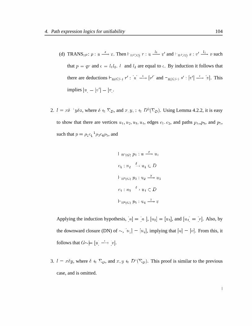
4. Path expression logics for unifiability 104
(d) TRANS�2 : p : u ��! v. Then `�2(G) r : u
l1�! v0 and `�2(G) s : v0 l2�! v such
that p = qr and � = l1l2. l1 and l2 are equal to �. By induction it follows that
there are deductions `�(G=�) r0 : [u]�
�! [v0] and `�(G=�) s0 : [v0]�
�! [v]. This
implies [u] = [v0] = [v].
2. l = x��1y�z, where � 2 �D, and x; y; z 2 D0(�D). Using Lemma 4.2.2, it is easy
to show that there are vertices u1; u2; u3; u4, edges c1; c2, and paths p1;,p3, and p5,
such that p = p1c�11 p3c4p5, and
`�2(G) p1 : ux�! u1
c1 : u2��! u1 2 D
`�2(G) p3 : u2y�! u3
c4 : u3��! u4 2 D
`�2(G) p5 : u4z�! v
Applying the induction hypothesis, [u] = [u1], [u2] = [u3], and [u4] = [v]. Also, by
the downward closure (DN) of �, [u1] = [u4], implying that [u] = [v]. From this, it
follows that G�j= [u]�
�! [v].
3. l = x�y, where � 2 �D, and x; y 2 D�(�D). This proof is similar to the previous
case, and is omitted.
a
4. Path expression logics for unifiability 105
The next lemma shows that membership in the unification closure � of a labeled di-
rected graph G is witnessed by a unification path labeled by a semi-Dyck sentence over the
edge labels of G.
Lemma 4.2.5 (Completeness of semi-Dyck-labeled unification paths)
Let G = h�V ;�D; V; L;Di be a labeled directed graph with unification closure �. If
G j= u � v, then there is a deduction `�2(G) p : ul
�! v such that l 2 D0(�D).
Proof By induction on �. There are five cases. In each case, we construct a proof such
that l 2 D0(�D).
1. REF�: u = v, `�2(G) � : u�
�! u by the REF�2 rule, and � 2 D0(�D).
2. INIT�: Let u ��! v 2 D, then `�2(G) u
��! v : u
��! v by the INIT�2 rule, and
l(u�
�! v) = �.
3. SYM�: Let G j= v � u. By the induction hypothesis, `�2(G) q : vl
�! u for some
l 2 D0(�D). inv(l) = l since l 2 D0(�D). By Lemma 4.2.3 (2), `�2(G) inv(q) : u l�! v.
4. TRANS�: Let u � v0, v0 � v, for some v0 2 V . By the induction hypoth-
esis, `�2(G) q : ul0�! v0 and `�2(G) r : v
0 l0�! v for some bidirectional paths q; r
in G such that l; l0 2 D0(�D). Then, by an application of the TRANS�2 rule,
`�2(G) qr : ull0�! v. Clearly, ll0 2 D0(�D).
4. Path expression logics for unifiability 106
5. DN�: u � v because there are vertices u0; v0 in V , and edges u0 ��! u (abbreviated
c) and v0 ��! v (abbreviated c0) in D such that u0 � v0. Then
`�2(G) c : u0 ��! u By INIT�2 1
`�2(G) c�1 : u
��1
�! u0 By SYM�2 2
`�2(G) q : u0 l�! v0 By the ind. hyp. 3
`�2(G) c�1q : u
��1l�! v0 By 2, 3 and TRANS�2 4
`�2(G) c0 : v0
��! v By INIT�2 5
`�2(G) c�1qc0 : u
��1l��! v By 4, 5 and TRANS�2 6
By the induction hypothesis in Step 3, l 2 D0(�D). Hence ��1l� 2 D0(�D).
a
Unification paths are complete with respect to connectivity in the �-quotient graph of
a directed labeled graph.
Lemma 4.2.6 (Unification path completeness)
Let G be a labeled directed graph G = h�V ;�D; L; V;Di. Let � denote the unification
closure of G. If G=�j= [u]�l0�! [v]�, then there is a deduction `�2(G) p : u
l�! v such
that l �D l0.
Proof The proof is by induction on `�(G=�) [u]l0�! [v]. By Lemma 4.2.1, it is sufficient
if we construct a deduction `�(G=�) [u]l0�! [v] for each case:
4. Path expression logics for unifiability 107
1. REF�: `�(G=�) [u]l0�! [v]: Then l0 = �, [u] = [v]. The result follows from
Lemma 4.2.5.
2. INIT�: `�(G=�) c : [u]��! [v]: Then [u]
��! [v] is an edge in G=� and � 2 �D.
Then, by the definition of a quotient graph, u0 ��! v0 2 D (abbreviated c) for some
u0 2 [u] and v0 2 [v]. Therefore
`�2(G) q : ul
�! u0 By Lemma 4.2.5, since [u] = [u0] 1
`�2(G) c : u0 ��! v0 By INIT�2 , since u0 �
�! v0 2 D 2
`�2(G) qc : ul��! v0 From 1 and 2 using TRANS�2 3
`�2(G) r : v0 m�! v By Lemma 4.2.5, since [v] = [v0] 4
`�2(G) qcr : ul�m�! v0 From 3 and 4 using TRANS�2 5
In steps (1) and (4), l; m 2 D0(�D) by the induction hypothesis.
Hence l�m �D(�D) �.
3. TRANS�: Straightforward application of inductive hypothesis. Omitted.
a
4. Path expression logics for unifiability 108
4.2.3 Computation of shortest unification paths
We have seen how unification source-tracking information may be encoded as unifi-
cation paths. One measure of the succinctness of this information is the length of the
unification paths encoding this information. Since unification paths are paths over a graph
whose labels are constrained by the context-free grammar D�(�) for an alphabet �, short-
est unification paths may be computed using the dynamic-programming-based context-
free-grammar shortest paths algorithms of Barrett et al. [5]. If G is a directed labeled graph
and L is a context-free language, then the context-free-grammar shortest path problem is
the problem of computing the shortest path from the set of all paths p in G between a given
source and destination vertex such that the label of p is a sentence in L. If L is specified by
a context-free grammar in Chomsky Normal Form (in which each production is of the form
A ! BC or A ! a for non-terminals A, B and C, and terminal a), then the algorithm of
Barrett et al. has time complexity O(jV j5jN j2jRj) where V is the vertices in G , N is the
set of non-terminals, and R the set of productions of the grammar.1 The efficiency may be
improved to O(jV j3jN jjRj) using Fibonnaci heaps.
For unification paths over a directed labeled graph G = h�V ;�D; V; L;Di, the gram-
marD�(�D) is of sizeO(�D) and may be transformed into a grammar in Chomsky Normal
Form whose set of non-terminals and productions is each of size O(�D). Thus, shortest
1The algorithm is unaffected if � productions of the form A! � are included in the grammar [66].
4. Path expression logics for unifiability 109
unification paths can be computed in O(jV j5j�Dj3) time, or O(jV j3j�Dj2) time using Fi-
bonnaci heaps.
4.3 Logic of unification paths
Unification paths may be constructed as “typed” path terms using the rules �U specified
in Figure 4.4. Judgements in �U are of the form p : ul
�! v, where G is a labeled directed
graph h�V ;�D; V; L;Di, p is a sentence over D [D�1, u; v are vertices in V , and l 2 ��D.
The judgement p : u l�! v asserts that p is a unification path in G whose label reduces to l
under D(�D) rewriting.
Theorem 4.3.1 (Soundness and Completeness of �U with respect to unification closure)
Let G = h�V ;�D; V; L;Di be a labeled directed graph. Let u; v be vertices in G. Then
1. (Soundness) If `�U (G) p : ul
�! v, then`�2(G) p : ul0�! v, l 2 ��D, and l = �D(�D)(l
0).
2. (Completeness) If `�2(G) p : ul0�! v such that l0 2 D�(�D), then`�U (G) p : u
l�! v,
such that l 2 ��D, and l = �D(�D)(l0).
Proof Soundness is by induction on �U deductions. Completeness is by induction on the
derivation of l0 using the rules of the grammar D�(�D). a
Paths computed by �U deductions are closed underD0 rewriting.
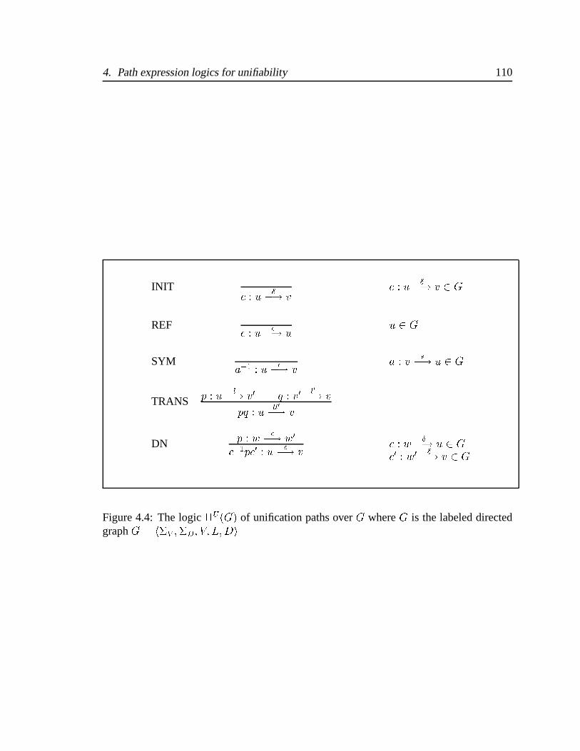
4. Path expression logics for unifiability 110
INITc : u
��! v
c : u��! v 2 G
REF� : u
��! u
u 2 G
SYMa�1 : u
��! v
a : v�
�! u 2 G
TRANS p : ul
�! v0 q : v0l0�! v
pq : ull0�! v
DN p : w�
�! w0
c�1pc0 : u�
�! vc : w
��! u 2 G
c0 : w0��! v 2 G
Figure 4.4: The logic �U(G) of unification paths over G where G is the labeled directedgraph G = h�V ;�D; V; L;Di
4. Path expression logics for unifiability 111
Lemma 4.3.1 (�U subject reduction)
Let G = h�V ;�D; V; L;Di be a labeled directed graph. Then `�U (G) p : ul
�! v and
p �!D0(D) q implies `�U (G) q : ul
�! v.
Proof By Lemma 4.3.1 (Soundness), `�2(G) p : um�! v, where m = l(p), and l =
�D(�D)(m). Since p��!D0(D) q, by Lemma 4.2.3 (3), `�2(G) q : u
n�! v, n = l(q),
and m �!D0(�D) n. Since m 2 D�(�D), by Lemma 4.1.2, m �D(�D) n. Therefore,
l = �D(�D)(m). By Lemma 4.3.1 (Completeness), `�U (G) q : ul
�! v. a
Example 4.3.15: In the graphG of Figure 4.1, `�U (G) b5a�13 : w4
g1�! x. `�2(G) b�14 b6 : w4
f1f2�! z,
but there is no�U deduction such that`�U (G) b�14 b6 : w4
f1f2�! z. Also, `�U (G) b�15 b5 : y
��! y,
and l(b�15 b5) = g�11 g1. `�2(G) b5b�15 : w4
g1g�1
1�! w4 but there is no corresponding deduction
in �U for the path b5b�15 . In other words, b5b
�15 is not a unification path even though its
normal form (under 2-sided cancellation) yields the unification path �. 3
There is a close resemblance of this logic to the inductive definition of unification clo-
sure� in Figure 3.3. The only apparent limitation is that SYM�U in Figure 4.4 is restricted
to leaves of deductions. This restriction is easily removed by replacing SYM�U rule by the
following “derived” rule:
SYM0 q : v�
�! uinv(q) : u �
�! v
4. Path expression logics for unifiability 112
This replacement is justified by the following lemma:
Lemma 4.3.2 `�U (G) q : u�
�! v implies `�U (G) inv(q) : v ��! u.
Proof By induction on the deduction `�U (G) q : u�
�! v. a
Based on this observation, we introduce the inverse operation directly as part of the
syntax of terms to obtain the logic PU , discussed in the next section.
4.4 Logic of Unification Path Expressions
We consider the logic of unification path expressions over a labeled directed graph
G = h�V ;�D; V; L;Di shown in Figure 4.5 whose terms are drawn from the term algebra
T (�Gr; D), where D is the set of labeled directed edges G. Judgements are of the form
p : ul
�! v where G is a labeled directed graph h�V ;�D; V; L;Di, p 2 T �(�Gr; D), and
l 2 ��D. `PU(G) p : ul
�! v denotes that there is a deduction in the logic PU whose last
step is p : u l�! v. Since the free monoid (D [D�1)� extended with the inverse function
inv is a �Gr-algebra, the function flatten from D to (D [D�1)� defined by
flatten(c) = c
uniquely extends to the homomorphism flatten : T �(�Gr; D) �! (D [D�1)�. We abbre-
viate flatten(p) by p. Thus, � = �, p�1 = inv(p), and pq = p q. The flatten function helps
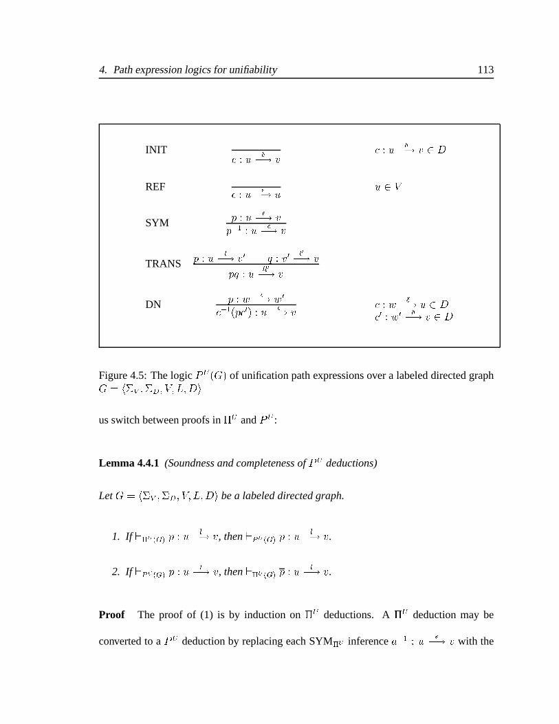
4. Path expression logics for unifiability 113
INITc : u
��! v
c : u��! v 2 D
REF� : u
��! u
u 2 V
SYM p : u�
�! vp�1 : u
��! v
TRANS p : ul
�! v0 q : v0l0�! v
pq : ull0�! v
DN p : w�
�! w0
c�1(pc0) : u�
�! vc : w
��! u 2 D
c0 : w0��! v 2 D
Figure 4.5: The logic PU(G) of unification path expressions over a labeled directed graphG = h�V ;�D; V; L;Di
us switch between proofs in �U and PU :
Lemma 4.4.1 (Soundness and completeness of PU deductions)
Let G = h�V ;�D; V; L;Di be a labeled directed graph.
1. If `�U (G) p : ul
�! v, then `PU (G) p : ul
�! v.
2. If `PU(G) p : ul
�! v, then `�U (G) p : ul
�! v.
Proof The proof of (1) is by induction on �U deductions. A �U deduction may be
converted to a PU deduction by replacing each SYM�U inference a�1 : u ��! v with the

4. Path expression logics for unifiability 114
following inference in PU .
c : u�
�! v 2 Dc : u
��! v
INIT
(c)�1 : v�
�! uSYM
The proof of (2) is by induction on PU deductions. Intuitively, each PU subdeduction
q : v�
�! u(q)�1 : u
��! v
SYM
may be replaced by the “derived” inference
q : v�
�! uinv(q) : u �
�! vSYM0
which in turn can be replaced with a deduction in �U . a
A unification path expression over a labeled directed graph G = h�V ;�D; V; L;Di is
said to have zero (0) or positive (+) parity if G `PU p : ul
�! v and l = � or l 2 �+D,
respectively. If x 2 f0;+g, we write P xuv(G) to denote the set of all unification path
expressions in G from u to v with parity x. We write P �
uv(G) to denote the set of all
unification path expressions in G from u to v.
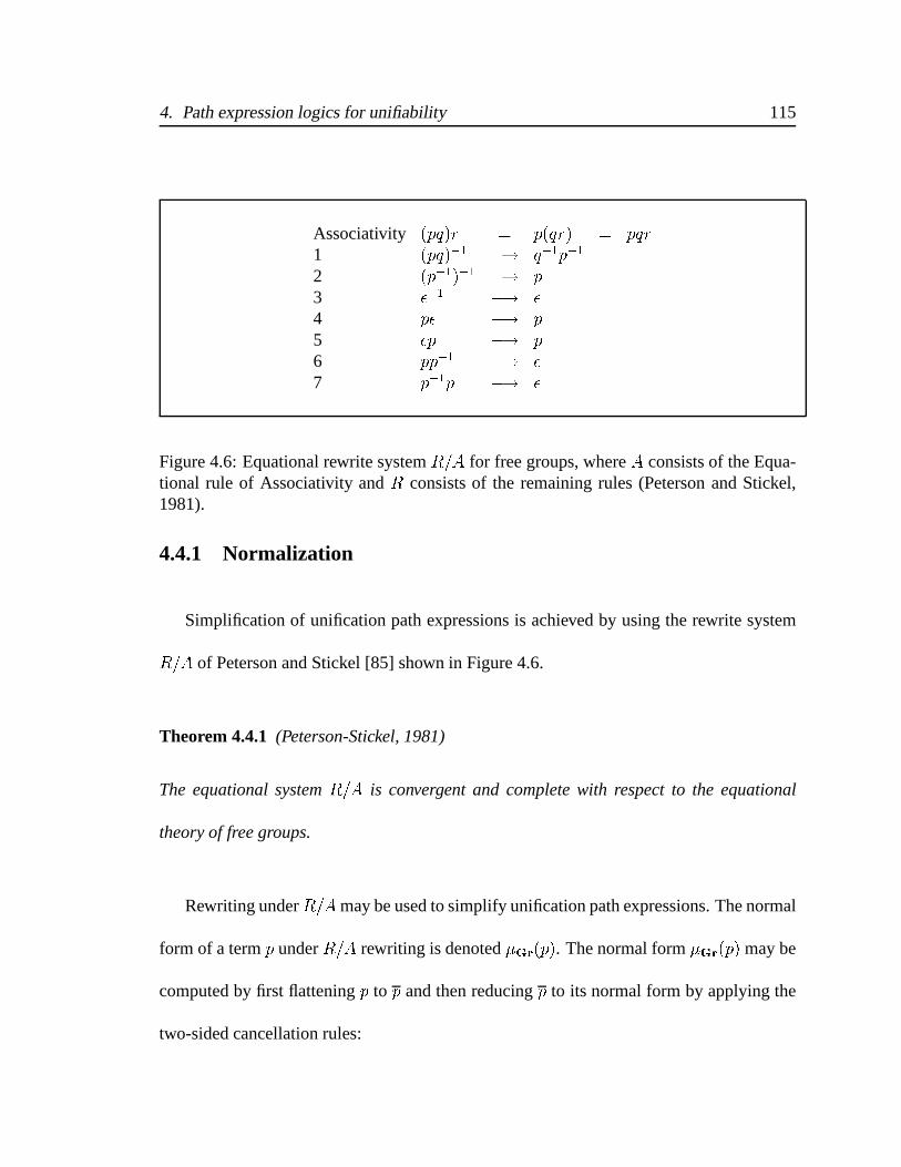
4. Path expression logics for unifiability 115
Associativity (pq)r = p(qr) = pqr1 (pq)�1 �! q�1p�1
2 (p�1)�1 �! p3 ��1 �! �4 p� �! p5 �p �! p6 pp�1 �! �7 p�1p �! �
Figure 4.6: Equational rewrite system R=A for free groups, where A consists of the Equa-tional rule of Associativity and R consists of the remaining rules (Peterson and Stickel,1981).
4.4.1 Normalization
Simplification of unification path expressions is achieved by using the rewrite system
R=A of Peterson and Stickel [85] shown in Figure 4.6.
Theorem 4.4.1 (Peterson-Stickel, 1981)
The equational system R=A is convergent and complete with respect to the equational
theory of free groups.
Rewriting under R=Amay be used to simplify unification path expressions. The normal
form of a term p under R=A rewriting is denoted �Gr(p). The normal form �Gr(p) may be
computed by first flattening p to p and then reducing p to its normal form by applying the
two-sided cancellation rules:
4. Path expression logics for unifiability 116
Lemma 4.4.2 (Decomposition of normal form computation)
If D is any set and p 2 T �(�Gr; D), then �Gr(p) = �D0(D)(p).
Proof Since p �Gr p, both p and p have the same normal form under R=A. Now, p is
flattened, which means every symbol in p is either c�1 or c, where c 2 D. Hence, the only
redexes in p are of the form cc�1 �!R=A � and c�1c �!R=A �. These redexes are exactly
those that can be reduced using D0(D). a
From this decomposition of normal form computation, it is straightforward to show that
the “type” of a unification path expression is preserved by its normal form.
Lemma 4.4.3 (PU Weak subject reduction)
Let G be a labeled directed graph and let `PU(G) p : ul
�! v. If p0 = �Gr(p), then
`PU (G) p0 : u
l�! v.
Proof By Lemma 4.4.1, if `PU (G) p : ul
�! v, then `�U (G) p : ul
�! v. By Lemma 4.4.2,
p0 = �D0(D)(p) and by Lemma 4.3.1, `�U (G) p0 : ul
�! v. a
Unification path expressions are not closed under one-step R=A rewriting, as illustrated
by the following example:
Example 4.4.16: (One-step rewriting in R=A)
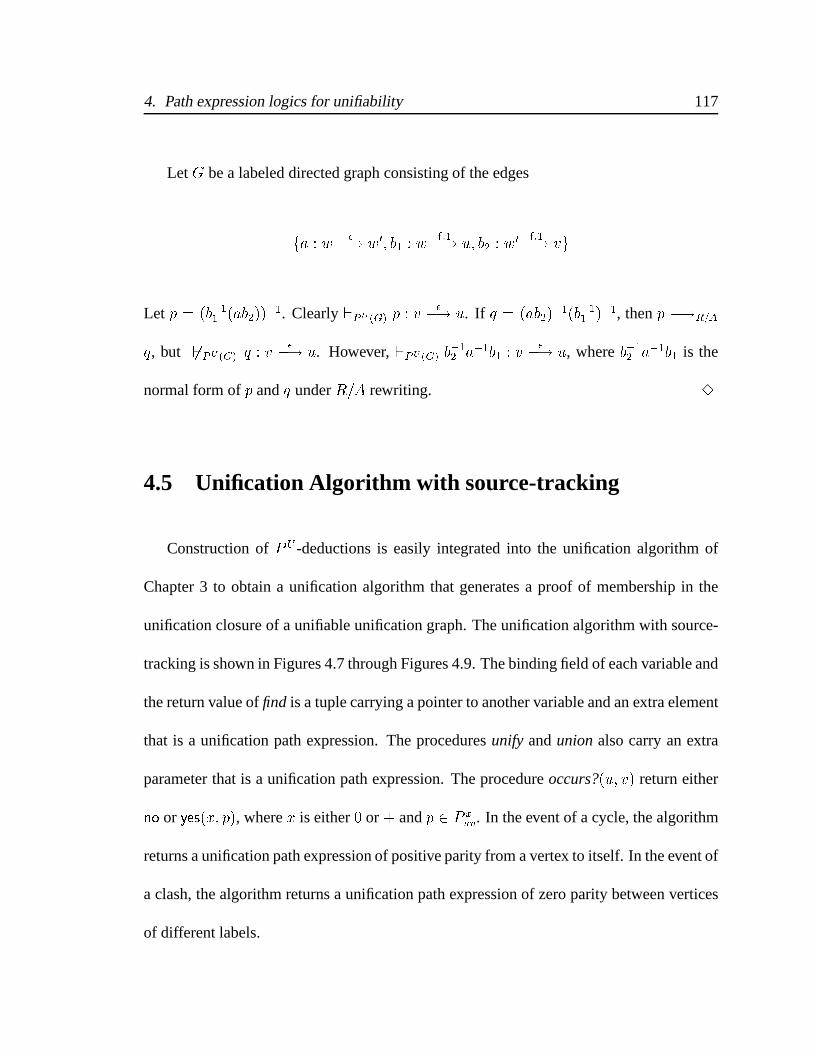
4. Path expression logics for unifiability 117
Let G be a labeled directed graph consisting of the edges
fa : w�
�! w0; b1 : wf:1�! u; b2 : w
0 f:1�! vg
Let p = (b�11 (ab2))�1. Clearly `PU(G) p : v
��! u. If q = (ab2)
�1(b�11 )�1, then p �!R=A
q, but 6`PU (G) q : v�
�! u. However, `PU(G) b�12 a�1b1 : v
��! u, where b�12 a�1b1 is the
normal form of p and q under R=A rewriting. 3
4.5 Unification Algorithm with source-tracking
Construction of PU -deductions is easily integrated into the unification algorithm of
Chapter 3 to obtain a unification algorithm that generates a proof of membership in the
unification closure of a unifiable unification graph. The unification algorithm with source-
tracking is shown in Figures 4.7 through Figures 4.9. The binding field of each variable and
the return value of find is a tuple carrying a pointer to another variable and an extra element
that is a unification path expression. The procedures unify and union also carry an extra
parameter that is a unification path expression. The procedure occurs?(u; v) return either
no or yes(x; p), where x is either 0 or + and p 2 P xuv. In the event of a cycle, the algorithm
returns a unification path expression of positive parity from a vertex to itself. In the event of
a clash, the algorithm returns a unification path expression of zero parity between vertices
of different labels.

4. Path expression logics for unifiability 118
1 procedure unify(v1; v2; m) =2 let hr1; p1i = find(v1) and hr2; p2i = find(v2)3 in if r1 = r2 then return4 else case r1:type; r2:type5 strict, strict: union(r1; r2; (p1)�1mp2)6 functor, strict: unify(v2; v1; (m)�1)7 strict, functor: let ans = occurs?(r2; r1)8 in case ans9 no: union(r1; r2; (p1)�1mp2)10 yes( ; q): fail(CYCLE; (p1)�1mp2q)11 functor, functor:12 if r1:L 6= r2:L then fail(CLASH; (p1)�1mp2)13 else14 union(r1; r2; (p1)�1mp2);15 for i = 1 to arity(r1:L) do16 unify(r1:child(i); r2:child(i); (b1)�1(p1)�1mp2b2)16a where b1 = edge(r1; r1:child(i))16b and b2 = edge(r2; r2:child(i))
Figure 4.7: Unification algorithm with source-tracking: procedure unify
17 procedure union(r1; r2; p) = r1:binding := hr2; pi
18 procedure find(v) =19 if unbound?(v) then return hv; �i20 else let hv0; pi = v:binding21 in let hr; qi = find(v0) in return hr; pqi
Figure 4.8: Unification algorithm with source-tracking: procedures union and find
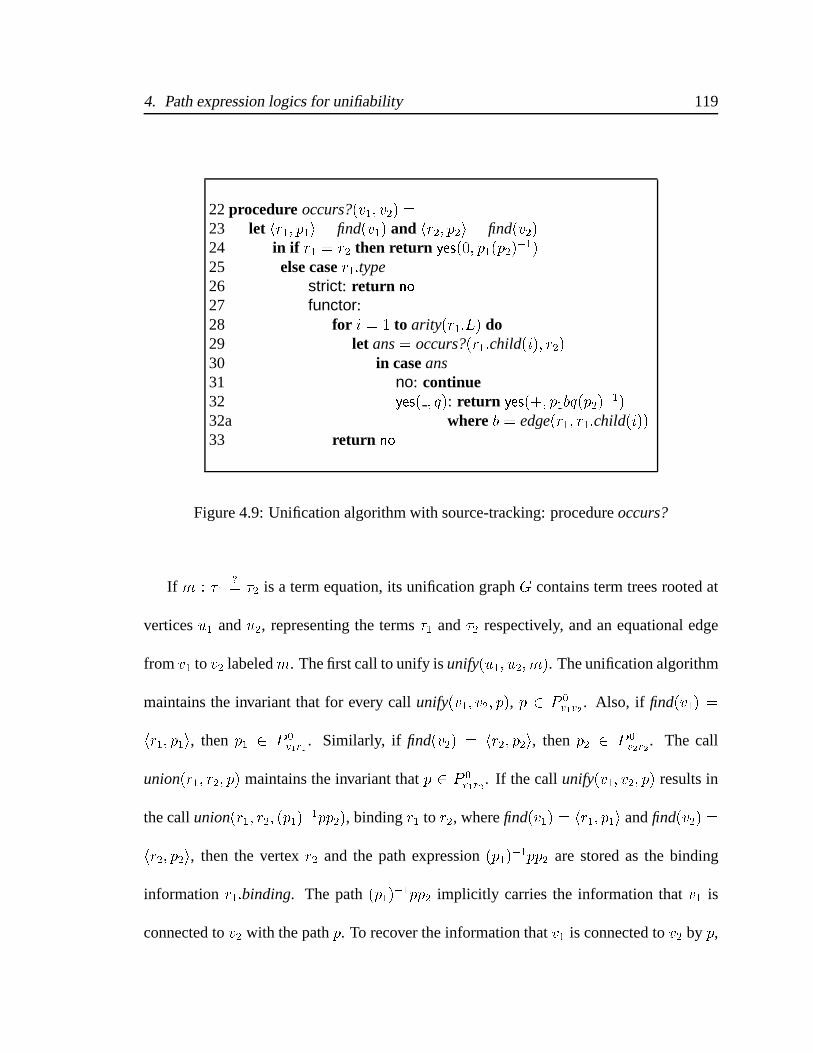
4. Path expression logics for unifiability 119
22 procedure occurs?(v1; v2) =23 let hr1; p1i = find(v1) and hr2; p2i = find(v2)24 in if r1 = r2 then return yes(0; p1(p2)
�1)25 else case r1:type26 strict: return no
27 functor:28 for i = 1 to arity(r1:L) do29 let ans = occurs?(r1:child(i); r2)30 in case ans31 no: continue32 yes( ; q): return yes(+; p1bq(p2)
�1)32a where b = edge(r1; r1:child(i))33 return no
Figure 4.9: Unification algorithm with source-tracking: procedure occurs?
If m : �1?= �2 is a term equation, its unification graph G contains term trees rooted at
vertices u1 and u2, representing the terms �1 and �2 respectively, and an equational edge
from v1 to v2 labeledm. The first call to unify is unify(u1; u2; m). The unification algorithm
maintains the invariant that for every call unify(v1; v2; p), p 2 P 0v1v2 . Also, if find(v1) =
hr1; p1i, then p1 2 P 0v1r1
. Similarly, if find(v2) = hr2; p2i, then p2 2 P 0v2r2
. The call
union(r1; r2; p) maintains the invariant that p 2 P 0r1r2
. If the call unify(v1; v2; p) results in
the call union(r1; r2; (p1)�1pp2), binding r1 to r2, where find(v1) = hr1; p1i and find(v2) =
hr2; p2i, then the vertex r2 and the path expression (p1)�1pp2 are stored as the binding
information r1:binding. The path (p1)�1pp2 implicitly carries the information that v1 is
connected to v2 with the path p. To recover the information that v1 is connected to v2 by p,
4. Path expression logics for unifiability 120
we simply compute the path expression following the binding pointers from v1 to v2, which
is done in three steps:
1. compute the path expression from v1 to r1 using find(v1), which is p1.
2. compute the path from r1 to r2 using find(r1), which is (p1)�1pp2.
3. compute the path from r2 to v2, which is (p2)�1.
The concatenation of these three path expressions, p1(p1)�1pp2(p2)�1, simplifies to
p using the rewrite rules R=A. All paths expressions manipulated by the algorithm are
unification path expressions. The yes answer returned by occurs? is now constructive,
and is of one of the following forms:
1. yes(0; q), implying that G=� j= [u]� = [v]�, and this is witnessed by the unification
path expression q 2 P 0uv.
2. yes(+; q) implying thatG=� j= [u]�+�! [v]� and this is witnessed by the unification
path expression q 2 P+uv.
Lemma 4.5.1 (Invariants for Unification algorithm with source-tracking)
Let G be a unification graph of a term equation �1?= �2 between the terms �1 and �2
represented by the term graphs rooted at vertices v1 and v2. Then the following invariants
are maintained by the unification algorithm:
4. Path expression logics for unifiability 121
1. For each call unify(u; v; p), `PU (G) p : u�
�! v.
2. For each call union(u; v; p), `PU (G) p : u�
�! v.
3. If find(u) = hv; pi, then `PU (G) p : u�
�! v.
4. If occurs?(u; v) = yes(x; p), then x 2 f0;+g, `PU(G) p : ul
�! v and l 2 �xN, where
�N is the set of context labels in G.
Proof The proof follows from a straightforward inspection of the path expressions con-
structed at each stage of the algorithm. a
The invariants show that at each stage, the unification algorithm with source tracking
not only constructs the unification closure � of a unification graph G, but also computes
witnesses of membership in the relation �. These witnesses are unification path expres-
sions. When unify fails, the algorithm presents a witness of the non-unifiability:
Corollary 4.5.1 Let � be a signature, and let G be a unification graph of a �-term equa-
tion �1?= �2 between the terms �1 and �2 represented by the term graphs rooted at vertices
v1 and v2. Then
1. If unify = fail(CY CLE; q), then `PU(G) q : ul
�! u for some vertex u in G and
label l 2 �+N
.
2. If unify = fail(CLASH; q), then `PU (G) q : w�
�! w0 for some functor vertices
w;w0 in G such that L(w1) 6= L(w2).
4. Path expression logics for unifiability 122
The cost of constructing unification path expressions at each point in the algorithm is
constant time per call to unify, find, union and occurs?, assuming structure sharing. Thus,
overall, the addition of source-tracking to the unification algorithm increases the runtime
of the unification algorithm by only a constant factor.
The process of normalization is orthogonal to the building of path expressions. It may
be performed once the unification path has been computed. It is easily seen that normaliza-
tion using R=A takes time proportional to the size of the term being normalized. Although
this normal form is not always of minimum size, its computation is considerably less ex-
pensive than the computation of the shortest unification path.
4.6 Summary
In this chapter we identified the set of unification paths that capture membership in the
unification closure of a unification graph. We introduced the deduction systems �U and PU
to compute these unification paths. Proofs in PU may be simplified by rewriting in R=A.
An extension of the unification algorithm that incorporates source-tracking by computing
deductions in PU was presented.
5
Error reconstruction in Curry-Hindley
Type Inference
This chapter develops a framework for applying the results of unification source-tracking
to the problem of diagnosing untypability in the Curry-Hindley [47] type system, ab-
breviated CH. The Curry-Hindley system defines a set of type rules for the lambda-
calculus [4, 21], and forms the basis for type systems of modern programming languages.
The problem of error reconstruction for CH type inference is simple, but fundamental
to the study of type inference in programs. It is the obvious basis for studying type error
information in statically-typed languages with type inference.
The framework we use is based on defining a domain of syntactic constraints and type
constraints. The rules of the type system determine a generating function that maps syn-
tactic constraints to type constraints.
123

5. Error reconstruction in Curry-Hindley Type Inference 124
Our framework may be used at two levels of program granularity. In the first, the
program is represented as a guarded flat system of syntax equations over locations (vertices
of the program syntax tree). Syntactic constraints (equations) are mapped by a generating
function to type equations, which are term equations whose variables range over program
locations. Source-tracking information is obtained as an inverse of the generating function
mapping syntax equations to type equations.
In the second approach, the domain of program locations is augmented with the special
location 2 denoting a “hole” or an irrelevant location. Terms built using this extended
domain are called weakenings. Weakenings are incomplete terms obtained by replacing
zero or more variables in a flat term by 2. Equations over incomplete terms provide a
finer-grained division of the program syntax graph and the unification graph.
There is a natural partial order over incomplete terms. This partial order induces a
partial order over the domain of weakenings of sets of type equations. The partial order
on weakenings of systems of type equations in turn corresponds to a simulation ordering
between the unification graphs of the systems of type constraints.
It is well-known that CH-typability is reducible to unification of terms encoding types
(see Hindley [46], Wand [109], or Cardelli [13]). The reduction of type inference to term
unification may be viewed as a process in which syntactic constraints generate type con-
straints that are then solved by unification. This leads to the notions of typability and

5. Error reconstruction in Curry-Hindley Type Inference 125
untypability of a syntactic constraint set. When programs are ill-typed, untypable syn-
tactic constraint sets are identified, rather than subexpressions. The ordering of syntactic
constraint sets leads to the notion of minimally untypable sets of syntactic constraints.
The approach outlined in this chapter relies on the properties of the constraint gen-
eration function and not on the solving of those constraints. Thus, the framework is in-
dependent of any specific type inference algorithm or data-structures. This is in contrast
to the algorithm-based techniques that collect source information, such as Wand’s algo-
rithm [109], techniques that “explain” source information by “debugging,” such as Duggan
and Bent [35] and Beaven and Stansifer [8], or “tracing” techniques specific to a particular
inference algorithm, such as Maruyama [69].
The form of the syntax and type constraints generated for CH are such that for every
non-trivial type constraint, it is possible to associate a syntactic constraint called its source.
This leads to a a source function that maps each type constraints back to its source.
There are several reasons why we focus on the study of the type inference problem
for the Curry-Hindley type system: first, the problem of type inference provides a useful
framework to which the results developed in the previous chapter can be applied. Second,
computation of type information is more interesting for type inference, where types of
variables are not declared and type information is completely inferred, than when variable
types are declared. Lastly, the Curry-Hindley type system has been very well studied as the
core of typed programming languages.

5. Error reconstruction in Curry-Hindley Type Inference 126
5.1 Type Systems
Some syntactically correct programs exhibit runtime behavior that includes application
of an operation to values not supported by the operation, like adding a number to a func-
tion value. A type system is a set of rules that associates expressions in a programming
language with syntactic entities called types. The type system usually decides what type,
if any, an expression can have. Type systems are used to identify a subset of programs that
make sense syntactically, but not semantically, and prevent their execution. A program is
executed only after it is verified to be well-typed according to the rules of the type system.
Type systems are usually part of the specification of a programming language.
A typing judgement or typing is an ordered triple A) e : � consisting of a set of hy-
potheses, A, an expression, e, and a type, � . It expresses the judgement that “under the
assumptions specified inA, the expression e has the type � .” A subset of these typing judge-
ments are identified as well-typings. The set of well-typings is usually defined by derivabil-
ity in the logic of the type system. Let X denote a type system. We write `X A) e : �
to denote a well-typing derivable in the logic of the type rules of X . An expression e is
well-typed in X if there are A and � such that `X A) e : � . In this case, we say that the
expression e has the type � under the assumptions A in the type system X . Otherwise, e is
said to be ill-typed or untypable in X . An expression that is well-typed in one type system
could be untypable in a different type system. Type inference or type reconstruction is the

5. Error reconstruction in Curry-Hindley Type Inference 127
process of taking an expression, and sometimes, a set of type assumptions, and construct-
ing a well-typing for that expression if it is typable, and reporting that the expression is
untypable otherwise.
Type systems are often specified using induction over program expressions. A well-
typing for an expression then guarantees a well-typing for all its subexpressions. The prob-
lem of computing a well-typing for an expression e may be reduced to solving a system of
constraints derived from the structure of e using the rules of the type system. The variables
in these constraints, called type variables, are place-holders for the types of the constituent
subexpressions of e. We state this principle as follows:
Proposition 5.1.1 e is typable under a type system X if and only if the system of type
constraints generated under the typing rules of X for e are solvable.
The structure of the system of constraints is of course dependent on the type system
X . Usually type constraints are encoded either as equations or inequations between types,
and these constraints are solved by term-unification and its many variants and extensions.
Instances of Proposition 5.1.1 are the reduction of CH-typability to unification of systems
of equalities between type terms (see for example, Hindley [46], Cardelli [13], Milner [75],
Wand [109]), the reduction of the Damas-Milner type system [28] for parametric polymor-
phism to unification, and the reduction of Milner-Mycroft typability [81] for polymorphic
recursion to semi-unification (Henglein [44], Kfoury et al. [58]).
5. Error reconstruction in Curry-Hindley Type Inference 128
When the system of type constraints generated for an expression e has a solution in the
form of a substitution s, often called a a substitution, the type of e is just the value of s(t),
where t is the type variable associated with e. On the other hand, when the system of type
constraints is unsolvable, the system of constraints and the expression e must be analyzed
to identify substructures of the expression e that generate subsystems of constraints that are
unsolvable.
The origins of type systems can be traced to the early twentieth century in the ef-
forts to provide a logical formalization of mathematics. Bertrand Russell introduced his
theory of “types” as a way of circumventing paradoxes in set theory and the formaliza-
tion of mathematics [93]. The simply-typed lambda calculus was introduced by Alonzo
Church [21]. The connection between unification and simply-typed lambda-calculus was
shown by Hindley [46, 47, 48]. A formal type system and type inference algorithms were
central to the design of the language ML(Milner et al. [77]), which was originally designed
as a meta language for theorem proving (Milner et al. [75]). More recently, type systems
have been used extensively for modeling safety, security, mobility, and correctness of soft-
ware systems. Survey articles on types include Cardelli and Wegner [15], Mitchell [78] and
Cardelli [14]. Recent texts devoted to the study of type systems in programming languages
include Schmidt [95] and Pierce [87].
5. Error reconstruction in Curry-Hindley Type Inference 129
5.2 Preliminaries: Partial Orders
The quality of source-tracking information can be characterized by imposing an order-
ing on the syntactic and type constraints derived from source-tracking. In this section, we
briefly state the definitions and facts related to partial orders that we require.
Given a set P and a binary relation vP on P , the pair (P;vP ) is a pre-order if vP is
reflexive and transitive. (P;vP ) is a partial order or poset, if vP is reflexive, transitive,
and antisymmetric. The relation x <P y is defined as “x vP y and y 6vP x.” x and y are
comparable under vP if x vP y or y vP x.
If (P;vP ) is a partial order, then for each subset Q of P , vP induces a partial or-
der hQ;vQi, where for each x; y 2 Q, x vQ y if and only if x vP y. Q is an an-
tichain if x vQ y implies x = y. If Q � P , then, the down-set of Q, denoted Q# is
fy 2 P j 9x 2 Q : y vP xg. If T is any set and ? is a special symbol not in T , then T?
denotes the flat poset hT [ f?g;vi, where x v y if and only if x = ? or x = y.
The partial order (P;vP ) induces an ordering on functions mapping into P . If A is any
set and f and g are functions from A to P , then g vP f if and only if for each a 2 A,
g(a) vP f(a).
If vP is a partial order, then the lower power-domain ordering induced by vP1 is the
preorder h2P ;vi where S 0 v S if and only if 8s0 2 S 0:9s 2 S : s0 vP s. It is easy to
1The lower power-domain ordering is also known as the Hoare ordering.
5. Error reconstruction in Curry-Hindley Type Inference 130
verify that S 0 v S if and only if S 0#� S#. Given a set Q � P , we are often interested
in the restriction of v to fS � P jS v Qg. If Q is finite, then every non-empty set S v Q
may be uniquely written asSni=1 ffxig#g where fx1; : : : ; xng is an antichain. We call this
the normal form of S. The orderingv becomes a partial order if sets with identical normal
forms are considered equal. It is easy to verify that if S; S 0 � P , and S 0 < S, where v is
the lower power-domain ordering induced by vP , then there is an s 2 S such that for all
s0 2 S 0, if s and s0 are comparable, then s0 <P s.
Let g : A �! B. If � 2 B and s 2 A, then s is a source for � under g if � = g(s).
A source function for g is a function h : B �! A such that g � h = IB2. If h is a source
function for g : A �! B, then for each � 2 B, h(�) is a source for � under g. A source
function for g exists if and only if g is onto. Also, if g is one-to-one and onto, then the
inverse g�1 of g is the unique source function for g.
A function g : A �! B, where (A;vA) and (B;vB) are partial orders, is monotone
if for each a; a0 2 A, a vA a0 implies g(a) vB g(a0). g is strictly monotone if a <A a0
implies g(a) <B g(a0). If � 2 B, then s 2 A is an imprecise source for � under g if
� vB g(s).
2h is more generally known as a section of g.
5. Error reconstruction in Curry-Hindley Type Inference 131
5.2.1 �-Graph simulations
The notion of simulation of errors in unification and type inference is captured by re-
lations on graphs called graph simulations. The idea of simulation is tied to the notion
of observable behavior. Informally, the observations on a graph consist of the labels on
vertices and directed edges of the graph. A graph simulation from a graph G0 to G shows
how the observable behavior of G0 may be captured by the observable behavior G.
Let G = hV; L;Di and G0 = hV 0; L0; D0i be �-graphs. A relation R � V 0 � V is a
simulation from G0 to G if for each (u0; u) 2 R
1. L(u) = L0(u)
2. If L0(u0) = ;, then u = u0
3. If u0 ��! v0, then there is a v 2 V such that u �
�! v and v0Rv.
R is a total simulation from G0 to G if for each v0 2 V 0, there is a v 2 V such that v0Rv.
G simulates G0, or G0 is simulated by G, written G0 v G if there is a total simulation
from G0 to G. The relation v is a pre-order.
Example 5.2.17: Let � = ff 7! 2g, let G = hV; L;Di and G0 = hV 0; L0; D0i be �-graphs,
where
1. V 0 = fw01; w0
2; n1g
5. Error reconstruction in Curry-Hindley Type Inference 132
2. L0 = fn1 7! ;; w01 7! ffg; w02 7! ffgg,
3. D0 = fw011�! n1; w
0
12�! n1; w
0
21�! n1g.
and let G = h�V ;�D; V; L;Di where
1. V = fw1; n1g
2. L = fn1 7! ;; w1 7! ffgg,
3. D = fw011�! n1; w
0
12�! n1g.
ClearlyG v G0. AlsoG0 v G because of the total simulation f(n1; n1); (w01; w1); (w0
2; w1)g
from G0 to G. 3
5.3 The CH type system: syntax and type rules
The main object of study in this chapter is the programming language� of�-expressions.
Let V be a denumerable set of program variables. The language � of �-expressions is de-
fined by the context free grammar
e := �x: e j x j @e e
where x ranges over V. The constructors � and @ are used for function construction and
application, respectively. � is known as a binding construct and in the expression � x: e,
5. Error reconstruction in Curry-Hindley Type Inference 133
the occurrence of x is called a binding occurrence.
The set of types � 2 is the free term-algebra over the signature � = f(!; 2)g and a
denumerable set N of type variables. Types may be described by the context-free grammar
� := t j �!�
in which t ranges over type variables and � ranges over types.
5.3.1 Abstract Syntax graphs representations of closed �-expressions
Usually �-expressions are represented as abstract syntax trees whose internal nodes are
labeled either by � or @, and whose leaves are labeled by variables. It is useful, however,
to consider term graph representations of �-expressions in which variable reference nodes
point directly to the binding variable occurrence in the case of �-bound variables. Such
terms graphs, called abstract syntax graphs (ASG’s), can be generated in a straightforward
manner from abstract syntax trees. This is best illustrated by an example.
Example 5.3.18: Let e be the �-expression
�0 x1: (@2 (@3 x5 x6) x4)
The subscripts refer to locations in the term graph. The ASG of e, shown in Figure 5.1,
5. Error reconstruction in Curry-Hindley Type Inference 134
is the pointed term graph hn0; Tei, where Te = hWe; Xe; bei is a term graph whose set of
functor vertices We is equal to fn0; n2; n3; n4; n5; n6g, the set of strict vertices Xe is fn1g,
and the function be is
n0 = �(n1; n2) n2 = @(n3; n4)
n3 = @(n5; n6) n4 = �var(n1)
n5 = �var(n1) n6 = �var(n1)
3
5.3.2 CH Type Rules
The CH type system, defined in Figure 5.2, relates expressions in � with types. The set
of CH-well-typings is defined as the least set closed under the rules in Figure 5.2. In these
rules, A is a finite function from V to types, called a type environment. Type environments
maintain hypotheses about types of variables possibly occurring free in an expression.
In our formulation of these rules, subscripts are used to identify parts of an expression.
It is useful to think of each vertex i in the parse tree of e as having an attribute that is the
type �i of that vertex. Each row in Figure 5.2 contains a rule name, a typing rule, and
a side condition that encodes a constraint between types of parts of the expression. Side
conditions express constraints on types that need to hold in addition to the antecedents of
a type rule in order to be able to infer the consequent of the type rule. Type constraints
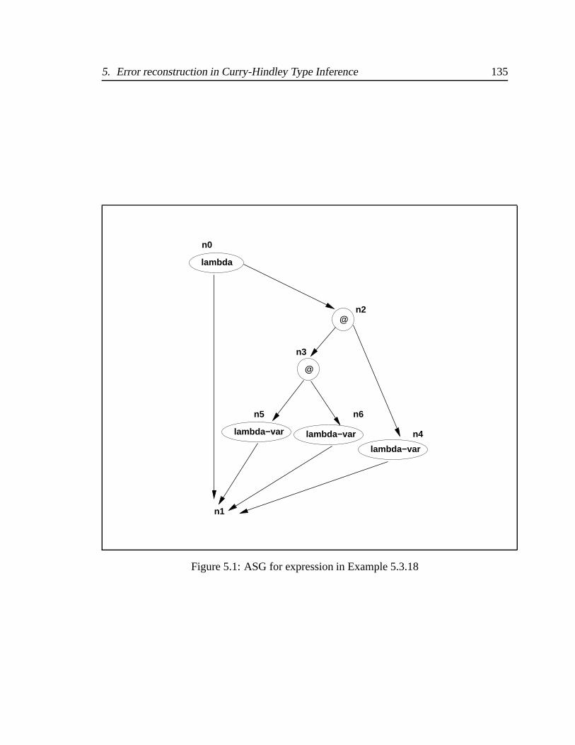
5. Error reconstruction in Curry-Hindley Type Inference 135
lambda
@
@
lambda−var
lambda−varlambda−var
n0
n2
n3
n5 n6
n4
n1
Figure 5.1: ASG for expression in Example 5.3.18

5. Error reconstruction in Curry-Hindley Type Inference 136
are expressed as type equations, which are term equations between pairs of type terms.
For the consequent of the rule to be a well-typing, the side condition must be satisfiable.
Note that the type system CH is syntax-directed: given an expression e, there is exactly
one rule in CH with an instance whose consequent contains e. The set of type equations
generated as side conditions by applying the corresponding type rules of Figure 5.2 to the
subexpressions of e is called the canonical set of type equations of e under CH, and is
denoted Ee.
A principal type of a closed expression e is a type of e from which all other types of
e may be derived by applying a substitution. The Curry-Hindley system admits principal
types. Hence, for any closed expression e, if e is typable in CH , then there is a type � such
that `CH ; ) e : � , and for any other � 0 such that `CH ; ) e : � 0, there is a substitution
� such that � 0 = �� . The type � is called the principal type of e. Principal types are
unique modulo renaming of variables. For example, `CH ; ) � x: x : t! t, and and t!t
is the principal type of � x: x (modulo renaming). Thus, `CH ; ) � x: x : � ! � , where
� = (t1 ! t1), and the type � ! � can be obtained from the type t!t by the substitution
t 7! � .
The problem of type inference was formulated and solved by Curry [26] and Hind-
ley [47] in the context of combinatory logic. The problem was independently discovered
and solved in a programming language context by Morris [79] and Milner [75]. Hindley
and Milner show how the principal type of a typable �-expression e is the mgu of the set
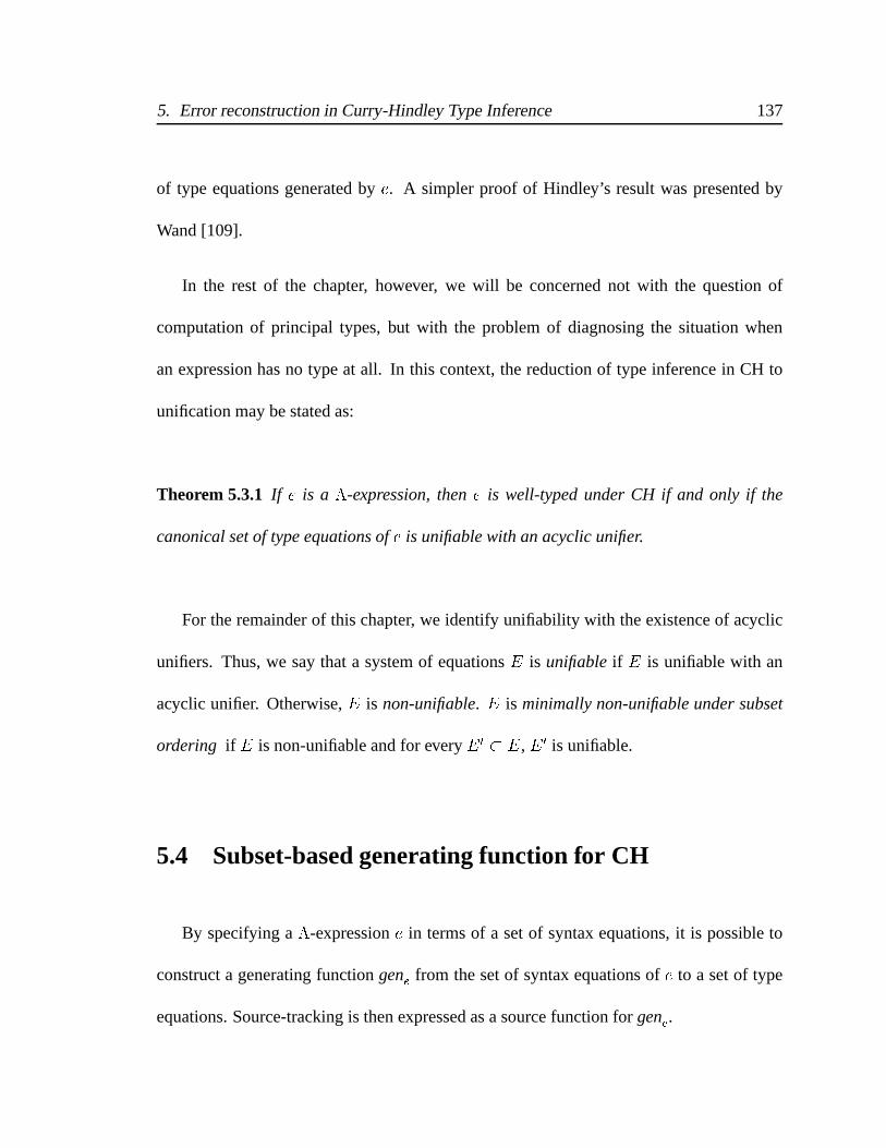
5. Error reconstruction in Curry-Hindley Type Inference 137
of type equations generated by e. A simpler proof of Hindley’s result was presented by
Wand [109].
In the rest of the chapter, however, we will be concerned not with the question of
computation of principal types, but with the problem of diagnosing the situation when
an expression has no type at all. In this context, the reduction of type inference in CH to
unification may be stated as:
Theorem 5.3.1 If e is a �-expression, then e is well-typed under CH if and only if the
canonical set of type equations of e is unifiable with an acyclic unifier.
For the remainder of this chapter, we identify unifiability with the existence of acyclic
unifiers. Thus, we say that a system of equations E is unifiable if E is unifiable with an
acyclic unifier. Otherwise, E is non-unifiable. E is minimally non-unifiable under subset
ordering if E is non-unifiable and for every E 0 � E, E 0 is unifiable.
5.4 Subset-based generating function for CH
By specifying a �-expression e in terms of a set of syntax equations, it is possible to
construct a generating function gene from the set of syntax equations of e to a set of type
equations. Source-tracking is then expressed as a source function for gene.
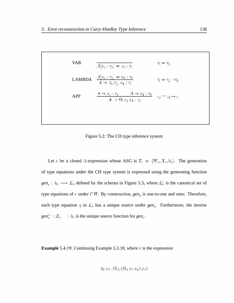
5. Error reconstruction in Curry-Hindley Type Inference 138
VARA[xj : �j]) xi : �i
�i = �j
LAMBDAA[xj : �j]) ek : �kA) �i xj: ek : �i
�i = �j!�k
APPA) ej : �j A) ek : �k
A) @i ej ek : �i�j = �k!�i
Figure 5.2: The CH type inference system
Let e be a closed �-expression whose ASG is Te = hWe; Xe; bei. The generation
of type equations under the CH type system is expressed using the generating function
gene : be �! Ee defined by the schema in Figure 5.3, where Ee is the canonical set of
type equations of e under CH . By construction, gene is one-to-one and onto. Therefore,
each type equation � in Ee has a unique source under gene. Furthermore, the inverse
gen�1e : Ee �! be is the unique source function for gene.
Example 5.4.19: Continuing Example 5.3.18, where e is the expression
�0 x1: (@2 (@3 x5 x6) x4)

5. Error reconstruction in Curry-Hindley Type Inference 139
gene(ni = �(nj; nk)) = ni?= nj ! nk
gene(ni = @(nj; nk)) = nj?= nk ! ni
gene(ni = �var(nj)) = ni?= nj
Figure 5.3: Schemas for the generating function gene mapping equations in be to typeequations in the canonical system Ee of type equations of e in the Curry-Hindley typesystem , where Te = hWe; Xe; bei is the ASG of the closed �-expression e.
the function gene is equal to:
n0 = �(n1; n2) 7! n0?= n1!n2
n2 = @(n3; n4) 7! n3?= n4!n2
n3 = @(n5; n6) 7! n5?= n6!n3
n4 = �var(n1) 7! n4?= n1
n5 = �var(n1) 7! n5?= n1
n6 = �var(n1) 7! n6?= n1
Figure 5.4 shows the unification graph representing Ee, along with labels and orienta-
tions for all edges in the graph. We let Ee denote both the system of type equations and the
unification graph representing them.
3
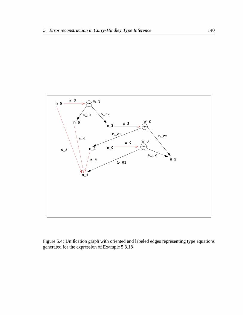
5. Error reconstruction in Curry-Hindley Type Inference 140
n_3
n_4
n_6
n_2
a_5
a_6
a_4
a_2
n_0a_0
b_31 b_32
b_21b_22
b_02
w_2
w_0
n_5
b_01
n_1
a_3 w_3
Figure 5.4: Unification graph with oriented and labeled edges representing type equationsgenerated for the expression of Example 5.3.18
5. Error reconstruction in Curry-Hindley Type Inference 141
5.4.1 Untypability of subsets of syntax equations
Let e be a closed �-expression whose ASG is the term graph hWe; Xe; bei. If e is
untypable, then the untypability of e may be traced to the non-unifiability of some subset
E � Ee of type equations, where Ee is the canonical set of type equations generated for
e. Since each type equation in Ee is generated from a syntax equation in be, the source of
untypability of an expression e can be traced to subsets of syntax equations of e.
Definition 5.4.2: Let e be an untypable �-expression whose term graph is hWe; Xe; bei and
gene be the generating function for e. The subset of syntax equations B � be is untypable if
and only if gene[B] is non-unifiable. B is minimally untypable if and only if B is untypable
and for all B0 � B, gene[B0] is unifiable. 2
The inverse function gen�1e immediately yields minimally untypable syntax equation
sets from minimally unifiable type equation sets:
Lemma 5.4.1 (Minimally untypable sets of syntax equations)
Let e be a decorated expression whose canonical set of type equations under CH is Ee. If
E � Ee is minimally non-unifiable, then gen�1e [E] is minimally untypable.
Proof Follows from the property that gene and is one-to-one and onto. a
The following example illustrates the extraction of untypable sets of syntax equations
from non-unifiable sets of type equations.
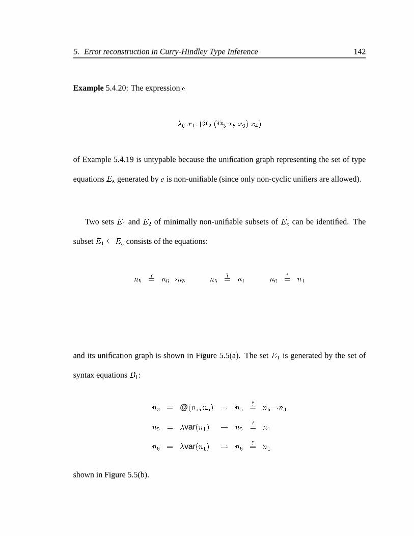
5. Error reconstruction in Curry-Hindley Type Inference 142
Example 5.4.20: The expression e
�0 x1: (@2 (@3 x5 x6) x4)
of Example 5.4.19 is untypable because the unification graph representing the set of type
equations Ee generated by e is non-unifiable (since only non-cyclic unifiers are allowed).
Two sets E1 and E2 of minimally non-unifiable subsets of Ee can be identified. The
subset E1 � Ee consists of the equations:
n5?= n6!n3 n5
?= n1 n6
?= n1
and its unification graph is shown in Figure 5.5(a). The set E1 is generated by the set of
syntax equations B1:
n3 = @(n5; n6) 7! n5?= n6!n3
n5 = �var(n1) 7! n5?= n1
n6 = �var(n1) 7! n6?= n1
shown in Figure 5.5(b).

5. Error reconstruction in Curry-Hindley Type Inference 143
n_3n_6
n_5a_3
a_5
a_6
b_31 b_32
w_3
n_1
(a)
@
lambda−varlambda−var
n3
n5 n6
n1
(b)
Figure 5.5: (a) the unification graph of the set of type equations E1 of Example 5.4.20 and(b) syntax equations B1 generating E1.
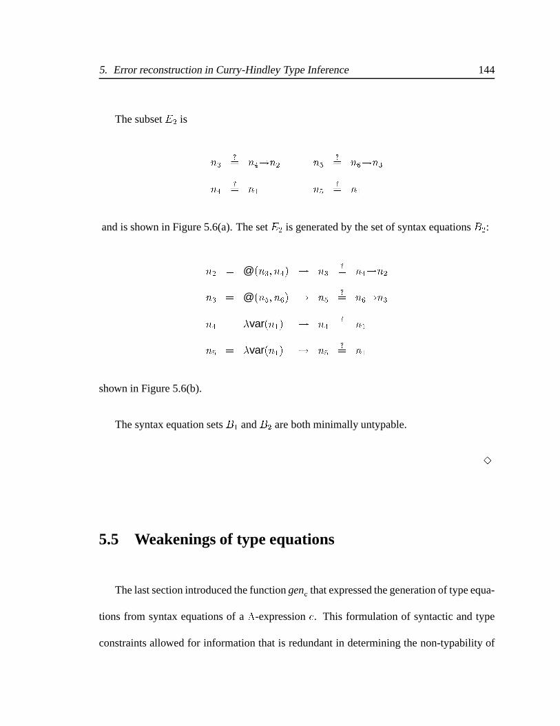
5. Error reconstruction in Curry-Hindley Type Inference 144
The subset E2 is
n3?= n4!n2 n5
?= n6!n3
n4?= n1 n5
?= n1
and is shown in Figure 5.6(a). The set E2 is generated by the set of syntax equations B2:
n2 = @(n3; n4) 7! n3?= n4!n2
n3 = @(n5; n6) 7! n5?= n6!n3
n4 = �var(n1) 7! n4?= n1
n5 = �var(n1) 7! n5?= n1
shown in Figure 5.6(b).
The syntax equation sets B1 and B2 are both minimally untypable.
3
5.5 Weakenings of type equations
The last section introduced the function gene that expressed the generation of type equa-
tions from syntax equations of a �-expression e. This formulation of syntactic and type
constraints allowed for information that is redundant in determining the non-typability of

5. Error reconstruction in Curry-Hindley Type Inference 145
n_3
n_4
n_6
n_2
n_5a_3
a_5
a_4
a_2
b_31 b_32
b_21b_22
w_3
w_2
n_1
(a)
@
@
lambda−var
lambda−var
n2
n3
n5
n4
n1
n6
(b)
Figure 5.6: (a) the unification graph of the set of type equations E2 of Example 5.4.20, and(b) the ASG of the syntax equations B2 generating E2.

5. Error reconstruction in Curry-Hindley Type Inference 146
an expression. For example, not all variables in the set of type equations E1 of Exam-
ple 5.4.20 contribute to the cyclicity of the unifier of E1. The source of the cyclicity is the
cycle involving the location variables n5, n6 and n1. The location n3 does not contribute
to this cycle, and should therefore not be part of the syntactic constraints generating the
cycle. Absence of locations from constraints is modeled by weakenings, obtained by re-
placing zero or more locations with a2. The symbol2may be thought of as a “hole,” each
occurrence of which representing an distinct anonymous location.
Recall from Chapter 3 that if N is a set of variables, and � is a signature, the set of
incomplete �-terms over N is the set of �-terms over N [ 2, where 2 denotes a special
variable not occuring in N . The set N [2may be considered a flat poset, with the ordering
x v y if and only if x = y or x = 2. The set of weak terms is the set of wellfounded �-
terms over N [2.
The set of weak term equations is the set of term equations over weak terms. The flat
poset v induces a partial order v on weak terms and weak term equations:
1. x v y, if x; y 2 N [2 and x = y or x = 2.
2. f(�1; : : : ; �n) v f(� 01; : : : ; �0
n), if �i; � 0i 2 T�(N [ 2) and �i v � 0i , 1 � i � n.
3. �1 = �2 v � 01 = � 02, if �1; �2; � 01; �0
2 2 T�(N [2), �1 v � 01 and �2 v � 02.
The partial order v on weak term equations induces a lower power-domain order over sets
of weak term equations: E v E 0 if for each � 2 E, there is an �0 2 E 0 such that � v �0.

5. Error reconstruction in Curry-Hindley Type Inference 147
Given a set E of weak term equations, the set of weakenings of E is defined to be the
downset E# of E. Weakenings are a generalization of linearizations (Le Chenadec [63]),
which are obtained by replacing any one occurrence of a variable occurring more than once
with a 2.
Example 5.5.21: For example, the set of weakenings of fn1 = n2 ! n3g is the set of
equations:
2 = 2! 2 n1 = 2! 2 2 = n2 ! 2 2 = 2! n3
n1 = n2 ! 2 2 = n2 ! n3 n1 = 2! n3 n1 = n2 ! n3
The set of weakenings of fn4 = n5g consists of the equations
2 = 2 n4 = 2 2 = n5 n4 = n5
3
The weakening relation on systems of type equations corresponds to the simulation
relation on their unification graphs.
Lemma 5.5.1 (Weakenings are graph simulations)
Let E 0 and E be flat sets of weak type equations such that E 0 v E. Let G0 and G be the
unification graphs of E 0 and E respectively. Then G0 v G.
5. Error reconstruction in Curry-Hindley Type Inference 148
Proof (Sketch) Let n00 = f(n01; : : : ; n0
k) be an equation in E 0. Then there is an equation
n0 = f(n1; : : : ; nk) in E such that n0i v ni, for 0 � i � k. The unification graph G0
of E 0 contains a vertex w0 and an edge from w0 to n0i provided n0i is not 2 for each i,
1 � i � k. Similarly, there is an equational edge from n00 to w0 if n00 is not 2. For the
equation n0 = f(n1; : : : ; nk) in E, the unification graph G of E contains a vertex w, and
an edge from w to nk provided nk is not 2. Similarly, there is an equational edge from n0
to w if n0 is not2. For each pair of equations n00 = f(n01; : : : ; n0
k) and n0 = f(n1; : : : ; nk),
we can construct the set f(w0; w)g [ f(n0i; ni) j n0
i 6= 2g. It is easy to verify that the union
of all such sets for each pair of equations hn00 = f(n01; : : : ; n0
k); n0 = f(n1; : : : ; nk)i yields
a simulation from G0 to G. a
5.6 Weakening-based generating function for CH
Let e be a closed �-expression, represented by the term graph of syntax equations
hWe; Xe; bei. Let Ee be the set of type equations generated for e under the type system
CH . The type equation generation function gene : be �! Ee may be extended to wgene,
whose domain is be# (the set of weakenings of be, also called weak syntax equations), and
whose range is Ee# (the set of weakenings of Ee, also called weak type equations). The
definition of wgene, shown in Figure 5.7 is identical to that of gene except that locations
range over We [ Xe [ f2g. It is easy to verify that wgene is strictly monotone and onto
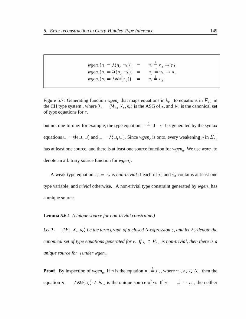
5. Error reconstruction in Curry-Hindley Type Inference 149
wgene(ni = �(nj; nk)) = ni?= nj ! nk
wgene(ni = @(nj; nk)) = nj?= nk ! ni
wgene(ni = �var(nj)) = ni?= nj
Figure 5.7: Generating function wgene that maps equations in be# to equations in Ee# inthe CH type system , where Te = hWe; Xe; bei is the ASG of e, and Ee is the canonical setof type equations for e.
but not one-to-one: for example, the type equation 2 ?= 2! 2 is generated by the syntax
equations 2 = @(2;2) and 2 = �(2;2). Since wgene is onto, every weakening � in Ee#
has at least one source, and there is at least one source function for wgene. We use wsrce to
denote an arbitrary source function for wgene.
A weak type equation �1 = �2 is non-trivial if each of �1 and �2 contains at least one
type variable, and trivial otherwise. A non-trivial type constraint generated by wgene has
a unique source.
Lemma 5.6.1 (Unique source for non-trivial constraints)
Let Te = hWe; Xe; bei be the term graph of a closed �-expression e, and let Ee denote the
canonical set of type equations generated for e. If � 2 Ee# is non-trivial, then there is a
unique source for � under wgene.
Proof By inspection of wgene. If � is the equation n1?= n2, where n1; n2 2 Ne, then the
equation n1 = �var(n2) 2 be# is the unique source of �. If n1 = 2 ! n3, then either
5. Error reconstruction in Curry-Hindley Type Inference 150
n1 = �(2; n3) 2 be# or n3 = @(n1;2) 2 be#, where n1; n3 2 We [ Xe. Since the term
graph Te is acyclic, exactly one of these equations are in be#. The case when n1 = n2 ! 2
is similar. a
5.7 Non-unifiability and untypability of weakenings
We now examine the structure of non-unifiable sets of weak type equations. A sys-
tem of weak type equations E is represented as an incomplete unification graph. We say
that a system of weak type equations E is unifiable if the incomplete unification graph
representing E is unifiable. The following property is easy to verify.
Lemma 5.7.1 (Weakening and non-unifiability)
Let E and E 0 be two systems of weak term equations such that E 0 v E. If E 0 is non-
unifiable, then E is non-unifiable.
Proof By Lemma 5.5.1, G0 v G where G0 and G are the unification graphs of E 0 and E
respectively. Let R be the simulation relation between the vertices of G0 and G. Hence for
each unification path p0 from u0 to v0 in G0, where u0; v0 are vertices in G0, there is a path p
in G from u to v such that u0Ru and v0Rv and the labels of p and p0 are equal. Therefore,
if G0 has a clash or a cycle witnessed by a path p0 then G has a clash or a cycle witnessed
by a path with the same label as that of p0. a

5. Error reconstruction in Curry-Hindley Type Inference 151
It follows that a system of weak term equations E is unifiable if and only if the normal
form of E is unifiable. A set of weak type equations E is minimally non-unifiable under v
if E is non-unifiable, and for all E 0< E, E 0 is unifiable.
We now examine the form of minimally non-unifiable sets of weak type equations and
the sets of syntax equations generating them. Let e be a closed �-expression with term
graph hWe; Xe; bei and canonical set of type equations Ee. Let wsrce be a source function
for wgene.
It is easy to verify that if E is minimally non-unifiable due to cyclicity, then the path
obtained by ignoring the edges incident on 2 variables in the unification graph of E is
a unification cycle. Furthermore, each equation in E contributes two strict vertices of
the cycle. Hence, every type equation in E is non-trivial and has the form n1?= n2,
n1?= 2! n2, or n1
?= n2 ! 2, where n1; n2 2 We[Xe. By Lemma 5.6.1, it follows that
if E is minimally non-unifiable, then every weak syntax equation in wsrce[E] is non-trivial
and has one of the following five forms: n1 = �var(n2), n1 = �(2; n3), n1 = �(n2;2),
n1 = @(n2;2), or 2 = @(n2; n3), where n1; n2; n3 2 Ne
5.7.1 Untypability of weak syntax equations
Given an expression e with term graph hWe; Xe; bei, the notion of untypability of sets
of weakenings of be can be defined in a manner analogous to the definition of untypability

5. Error reconstruction in Curry-Hindley Type Inference 152
of sets of syntax equations that are subsets of be.
Definition 5.7.3: Let e be a �-expression whose term graph is hWe; Xe; bei. A set of weak-
enings S v be is untypable if wgene[S] is non-unifiable. S v be is minimally untypable if
S is untypable and for all S 0 < S, wgene[S] is unifiable. 2
The result of Lemma 5.4.1 about deriving minimally untypable syntax equation sets as
sources of minimally non-unifiable subsets of Ee is valid if we replace the subset ordering
�with the lower power-domain ordering induced by the weakening partial orderv on term
equations.
Lemma 5.7.2 (Minimally untypable sets of weak syntax equations)
Let e = hNe; bei be a decorated expression whose canonical set of type equations is Ee.
Let wsrce be a source function of e with respect to wgene. If E v Ee is a minimally
non-unifiable antichain, then wsrce[E] is minimally untypable.
Proof Let S = wsrce[E]. S is a source for E because wgene[S] = E. To show that S
is minimally untypable, we need to show that if S 0 < S, then E 0 = wgene[S0] < E. That
is, we need to show that E 0 v E and E 6v E 0. Clearly, E 0 v E. Assume, for the sake of
contradiction, that E v E 0. Since S 0 < S, it follows that S 6v S 0. S 6v S 0 means that there
is an s 2 S such that for all s0 2 S 0, s and s0 are comparable implies s0 < s.
Let y = wgene(s). Since E v E 0, let y0 2 E 0 such that y v y0. Let y0 = wgene(s0),
where s0 2 S 0. There are two cases:
5. Error reconstruction in Curry-Hindley Type Inference 153
� s and s0 are comparable: Then s0 < s. Hence y0 < y, since wgene is strictly mono-
tone. But this contradicts the assumption that y v y0.
� s and s0 are non-comparable. Since S 0 v S, let s00 2 S : s0 v s00. Let y00 =
wgene(s00). Since wgene is monotone, y0 v y00. Hence, we have y v y0 v y00,
which implies y v y00. Since E is an antichain, it follows that y = y00 and hence
s0 v s00 = s, contradicting the assumption that s and s0 are non-comparable.
a
Example 5.7.22: Continuing Example 5.3.18, where e is �0 x1: (@2 (@3 x5 x6) x4), and
the unification graph of Figure 5.4 Ee is cyclic, the cycle C1 equal to a3b31a6a�15 consists
of the path segments a3b31, a6 and a�15 . The first segment corresponds to the weakening
n5 = n6!2 of the type equation n5 = n6!n3. The second and third correspond to the
type equations n6 = n1 and n5 = n1. Thus, the cycle C1 corresponds to the minimally
non-unifiable set of weak type equations:
n5?= n6!2
n6?= n1
n5?= n1
The cycle C1 is shown in Figure 5.8. The weakening n5 = n6!2 is generated from
the weakening 2 = @(n5; n6) of the syntax equation n3 = @(n5; n6) using the generating

5. Error reconstruction in Curry-Hindley Type Inference 154
function wgene. The equations n6 = n1 and n5 = n1 are generated from the syntax
equations n6 = �var(n1) and n5 = �var(n1), respectively. Thus the following set S1 of
weak syntax equations together generates the cycle C1:
2 = @(n5; n6) 7! n5?= n6!2
n6 = �var(n1) 7! n6?= n1
n5 = �var(n1) 7! n5?= n1
The term graph of S1 is shown in Figure 5.8.
Similarly, the cycle C2 equal to a3b32a2b21a4a�15 and shown in Figure 5.9 corresponds
to the minimally non-unifiable set of weakenings
n3?= n4!2 n5
?= 2!n3
n4?= n1 n5
?= n1
The cycle C2 is generated by the following set S2 of syntax equation weakenings:
2 = @(n3; n4) 7! n3?= n4!2
n3 = @(n5;2) 7! n5?= 2!n3
n4 = �var(n1) 7! n4?= n1
n5 = �var(n1) 7! n5?= n1
and is graphed in Figure 5.9.
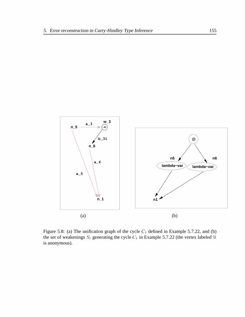
5. Error reconstruction in Curry-Hindley Type Inference 155
n_6
n_5a_3
a_5
a_6
b_31
w_3
n_1
(a)
@
lambda−varlambda−var
n5 n6
n1
(b)
Figure 5.8: (a) The unification graph of the cycle C1 defined in Example 5.7.22, and (b)the set of weakenings S1 generating the cycle C1 in Example 5.7.22 (the vertex labeled @is anonymous).
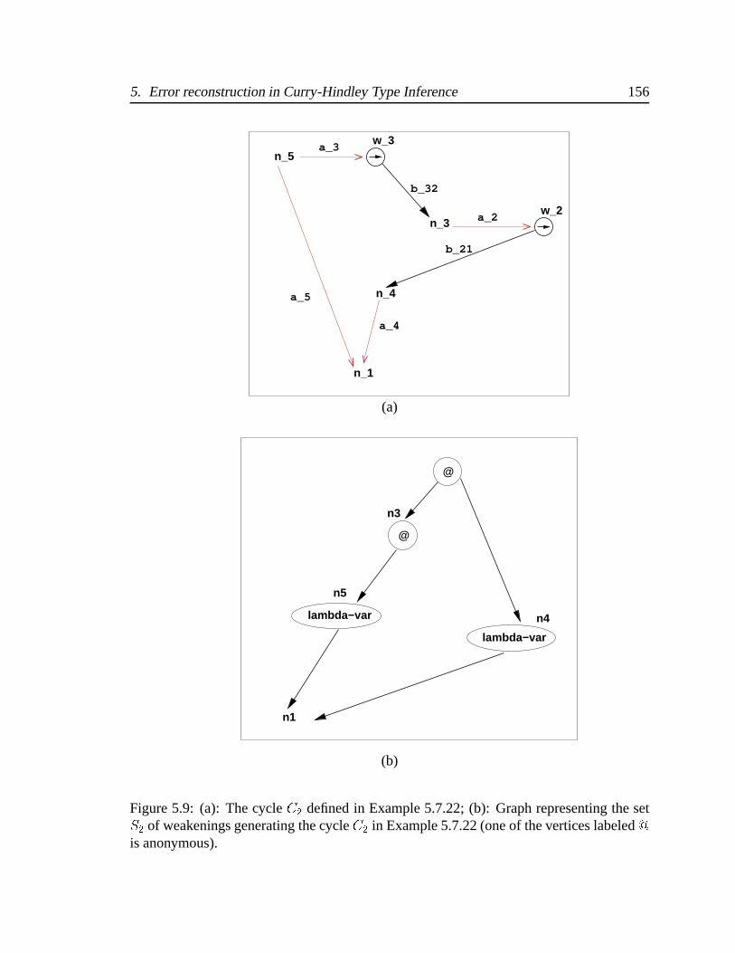
5. Error reconstruction in Curry-Hindley Type Inference 156
n_3
n_4
n_5a_3
a_5
a_4
a_2
b_32
b_21
w_3
w_2
n_1
(a)
@
@
lambda−var
lambda−var
n3
n5
n4
n1
(b)
Figure 5.9: (a): The cycle C2 defined in Example 5.7.22; (b): Graph representing the setS2 of weakenings generating the cycle C2 in Example 5.7.22 (one of the vertices labeled @is anonymous).

5. Error reconstruction in Curry-Hindley Type Inference 157
It is easy to verify by inspection that S1 and S2 are minimally untypable. 3
5.8 Properties of source functions
It is not clear whether generating functions for type systems other than the CH type
system considered here will enjoy the property that every subsystem of its canonical system
of type equations will have a source. There are two properties of generated type equations
that are necessary for the existence of source functions. We discuss these properties next.
5.8.1 Locality
Let s denote a syntax equation and let vars(s) denote the set of non-2 variables occur-
ring in s. The generating functions gene and wgene of the CH type system have the property
that vars(gene(s)) � vars(s) and vars(wgene(s)) � vars(s). We call this the locality prop-
erty. If locality is violated for some generating function on some domain and range, source
information may not be available. For example, if ge is the generating function
n0 = f(n1) 7! n0?= n1 ! n2
2 = f(n1) 7! 2?= n1 ! n2
n0 = f(2) 7! n0?= 2! n2
2 = f(2) 7! 2?= 2! n2
5. Error reconstruction in Curry-Hindley Type Inference 158
of some hypothetical type system, then vars(g(n0 = f(n1))) 6� vars(n0 = f(n1). The
weakening n0 = n1 ! 2 has no source. On the other hand, n0 = n1 ! 2 has an
imprecise source n0 = f(n1), because n0 = n1 ! 2 is weaker than n0 = n1 ! n2, which
is equal to g(n0 = f(n1)).
The locality property is not satisfied for type systems that involve the generation of
“fresh” type variables, as in the Damas-Milner polymorphic type system [28]. Understand-
ing the origin of these fresh (or non-local) variables is an additional complexity in the
source-tracking of polymorphic type systems.
5.8.2 Linearity
A syntactic entity s is linear if there are no repeated occurrences of any non-2 variables,
otherwise s is non-linear. For example, f(n1; n1), and n1 = f(n2; n2) are non-linear
whereas f(n1; n2) and n1 = f(n2; n3) are linear. Each syntax equation in the term graph
for a �-expression is linear. The generating functions considered in this chapter preserve
the linearity of the entities on which they operate. Since each syntax equation generates a
linear type equation, all the generated type equations in Ee and their weakenings, are linear
entities.
If the linearity property is violated, precise source information may not exist. For ex-
ample, if a generating function g for some type system maps a linear syntax equation s
5. Error reconstruction in Curry-Hindley Type Inference 159
equal to n0 = f(n1) to a non-linear indexed type equation � given by n0 = n1 ! n1, then
the weakening n0 = n1 ! 2 has only an imprecise source n0 = f(n1).
It is possible for a type system to have rules that generate non-linear type equations
as side conditions. This is certainly true in polymorphic type systems like Damas-Milner,
where, for example, instantiating the type of a polymorphic identity function at a location
n may yield the non-linear type equation n = t ! t, where t is a type variable. Again,
non-linearity makes the tracking of source information more difficult.
5.9 Summary
In this chapter, we introduced a generating-function based framework for solving the
problem of source-tracking for type inference. Generating functions for the Curry-Hindley
type system (CH) were defined. We presented two different ways of associating source
information with type constraints by considering different orderings between the domains
and ranges of the generating function. We defined the notion of minimal untypability for
sets of syntax equations and their weakenings, and showed how these sets can be extracted
given minimally non-unifiable sets and weakenings of type equations and weakenings for
the generating functions defined for CH. Finally, we considered how the properties of lo-
cality and linearity determine the applicability of these results to other type systems.
6
Conclusions and Future Work
The initial goal of this research was to build a system to facilitate the diagnosis of oth-
erwise hard to comprehend type error messages in languages like ML. Implementations of
some of the published and well-known type error diagnosis algorithms such as Wand [108],
revealed that these algorithms were sometimes not effective in practice, probably because
they lacked a sound formal basis. The formal basis for type inference is unification, and
this thesis has analyzed the reasons for non-unifiability and tied this information back to
the fragments of the program source associated with the non-unifiable equations.
6.1 Conclusions
We have shown how the debugging of term unification and type inference may be ap-
proached as exercises in proof construction in an appropriate logical system. By expressing
160

6. Conclusions and Future Work 161
the proof of non-unifiability as a context-free path in the unification graph, we have shown
how optimal proofs of non-unifiability may be computed in polynomial time. On the other
hand, construction of a single, not necessarily optimal proof can be done by a simple, yet
practical extension of the standard unification algorithm. Since this proof may contain re-
dundant inferences, a rewriting technique for simplifying proofs is introduced. The use
of a rewriting technique simplifies the proofs generated by the diagnostic unification algo-
rithm. Simplification of debugging information seems to be a novel application of rewrite
systems.
As an application of diagnostic unification, this thesis presented a solution to the prob-
lem of tracking the source of type inference. This was based on a framework of generating
functions mapping program source code to subsystems of type equations. The framework
was applied to the problem of type inference in the Curry-Hindley system. The main in-
sight developed here is that source-tracking is more accurately expressed as constraints
between program subexpressions expressed as first-order logic predicates over vertices of
the program syntax tree, rather than as a collection of subtrees or locations in a program.
There appear to be no substantial experimental studies comparing alternative approaches
to unification failure diagnosis. Results are needed to quantify the utility of the approach
outlined in this thesis in comparison with other approaches. One important experiment
consists of comparing the size of proofs computed by the algorithms proposed in this thesis
with that of the the shortest path algorithms suggested by Barret et al. [5], and algorithms
6. Conclusions and Future Work 162
for minimal proofs suggested in Cox [25], Chen [17], and Gandhe [38] for realistically
sized unification problems. The simplicity of our proposed modification to the unification
algorithm, both in terms of complexity considerations and ease of implementation, should
be factored into any comparative analysis.
There are three directions in which the present research may be used or extended: im-
mediate theoretical and practical extensions of the the current work, applications, and inte-
gration with automatic debugging.
6.2 Immediate Extensions
6.2.1 Damas-Milner Type Inference
An important extension to the framework for diagnosing Curry-Hindley type inference
is the computation of source-tracking information for type inference in the Damas-Milner
type system. The Damas-Milner type system [27, 28] is at the heart of the programming
language ML [41, 77]. A distinguishing feature of ML is that it not only supports type
inference at compile-time, but allows one to write polymorphic functions that can be re-
used to operate on different data-types, a feature typically found in untyped functional
languages like LISP. This is achieved by introducing a new variable-binding let construct
with a variable, an expression and a body. The let-bound variable is assigned a type in
such a manner that each reference to it in the body is associated with a fresh instance of the
6. Conclusions and Future Work 163
type of the variable. For example, in the ML program letf = �x:x in :::f(2):::f(true), the
function f is used with two different types num!num and bool!bool. Each of these types
is an instantiation of the polymorphic type 8t:t!t attributed to the binding occurrence of
f . The polymorphic type 8t:t!t is parameterized by the type variable t. Languages that
permit the definition and use of functions with parameterized polymorphic types are said to
support parametric polymorphism and their typing disciplines are described by parametric
polymorphic type systems, or polymorphic type systems for short. Other languages with
polymorphic type disciplines include Haskell [50, 86] and Miranda [101]. More recently,
there have been proposals to add polymorphic types to Java [12, 98] and compile Standard
ML to Java [73].
Type inference in the Curry-Hindley type system involves deriving and solving equa-
tional constraints between type variables associated with program locations. The Curry-
Hindley type system allows a clear separation between the generation of the type con-
straints and their solution. Type inference in Damas-Milner is implemented by Milner’s al-
gorithm W [75]. The implementation of W , however, makes such a separation impossible
because the generation of equations is dependent on the solution of a subset of previously
generated equations. An important aspect of Damas-Milner type inference is the general-
ization and instantiation of type expressions. Generalization of a type expression � in a
type environment A results in the polymorphic type 8~�� , where ~�, the set of type variables
in � not occurring free in A, is called the set of generic type variables in � relative to A.
6. Conclusions and Future Work 164
The non-generic variables of 8~�:� are the variables vars(�)� ~�. Instantiating a polymor-
phic type 8~�:� consists of creating a copy of � by replacing each generic variable � by a
fresh variable �0, and leaving each non-generic variable unchanged. The new type variables
are not directly associated with any program location. There are two questions relevant to
source tracking of polymorphic types. The first consists of locating parts of the program
that contribute to a type variable being marked as generic or non-generic. The second con-
sists of computing relevant source information to track the origin of freshly generated type
variables.
We briefly summarize a plausible approach to source-tracking Damas-Milner type in-
ference. Most of the details of this approach have been worked out and will be reported
elsewhere in the future. The approach is based on exploiting the observation, noted by
Mitchell [78], that the let construct of ML is primarily an abbreviation mechanism, and
unfolding the let binding at each occurrence of a let-bound variable reference preserves
the static (type) and dynamic (valuation) semantics of an ML expression (see Kanellakis
et al. [56]). Thus type variables created in W by type-variable instantiation are exactly
those type variables that are associated with the new locations created by unfolding of
let-bindings at their point of reference. The expression obtained by unfolding all the let-
bindings in an expression e is called the letvar normal form of e. letvar normal forms have
no let-bound variable references and their type inference problem may be expressed using a
6. Conclusions and Future Work 165
trivial extension of the Curry-Hindley type system. It is not practical to solve the type infer-
ence problem of e by reducing it to its letvar normal form because the normalization could
likely result in an exponentially larger program. However, the type equations generated for
the letvar normal form of e can be understood without the machinery of polymorphic types
and may therefore be considered a canonical simplification of the type inference problem
of e. Source-tracking information may be expressed as a path embedding from the term
graph of the type of an expression e computed by W to the unification graph of the set of
canonical type equations generated by the letvar normal form e of e in the trivial extension
of the Curry-Hindley system. The source-tracking algorithm tracks the origin of each type
variable and equation generated by W to a unification path in the unification graph of the
equations generated by the type inference of e. The source-tracking algorithm unfolds only
those parts of the let-binding that are necessary for generating the path in the canonical set
of type equations for e, thus preventing unnecessary unfolding.
6.2.2 Equational and Semi-unification
We have solved unification diagnosis for unification in the empty equational theory,
which is denoted ;-unification. There are two important generalizations of ;-unification:
equational unification and semi-unification. Equational unification, or E-unification is
the problem of unifying terms modulo a set of equational identities E. For example, the
terms f(b; a) and f(a; b), where f is a functor and a; b are constants, do not unify under

6. Conclusions and Future Work 166
-unification, but do unify if we consider unification modulo commutativity (allowing use
of f(x; y) = f(y; x) as an equational axiom). E-unification is a natural generalization of
;-unification and is used extensively in automated deduction and rewrite systems. Devel-
oping a general framework for diagnosing E-unification, or specific cases of E-unification
(associativity and commutativity, for example) is an open issue.
The unification problem solves equations of the form �?= � 0 by finding a substitution
s such that apply(s; �) = apply(s; � 0). Given two terms � and � 0 we say that � � � 0 if
there is a substitution � such that apply(s; �) = � 0. A term inequation I is a pair �?�
� 0. A substitution s is a semi-unifier for I if and only if apply(s; �) � apply(s; � 0). A
system of equations and inequations hE; Ii is solved by a semi-unifier s if s is a unifier
for each equation in E and a semi-unifier for each inequation in I . Type inference in
the presence of polymorphic recursion is reducible to semi-unification [44, 57], which is
undecidable. Construction of a logic for semi-unification is an open problem. Such a
logic would provide a formal basis for source-tracking of type inference in the presence of
polymorphic recursion.

6. Conclusions and Future Work 167
6.3 Other Applications
Since unification is at the core of several applications, the source-tracking unification
algorithm can form the basis of debugging and source information for a variety of applica-
tions. We briefly mention two applications: Prolog debugging and soft typing.
6.3.1 Source-tracking of Prolog programs
There have been multiple proposals for Prolog debugging systems [33, 82]. The state
of a Prolog program includes the current set of choice points, which determines the set of
term equations unified so far, and the trail of bindings made so far, which determines the
solution to those equations. The Prolog debugging problem can then be cast as a unification
diagnosis problem. The unification diagnosis information can then be applied to isolate a
Prolog program slice from these two pieces of information.
6.3.2 Soft-typing
Soft-typing [37] is a framework used to indicate the certainty of some type errors and
the possible presence of others in programs in latently typed languages like Scheme. Soft
typing transforms the original program by inserting runtime checks at points where the type
of the program can not be inferred. The resulting program conforms to the static typing
regime of the soft typing system, while preserving the runtime behavior of the original
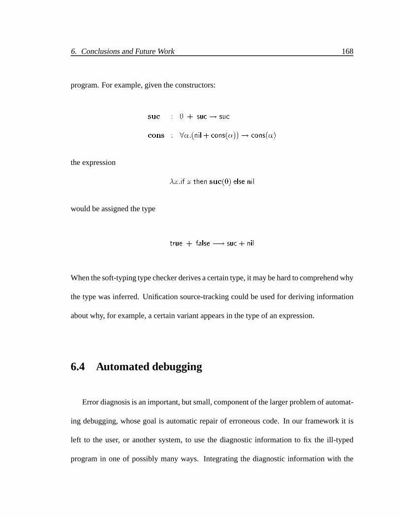
6. Conclusions and Future Work 168
program. For example, given the constructors:
suc : 0 + suc ! suc
cons : 8�:(nil+ cons(�))! cons(�)
the expression
�x:if x then suc(0) else nil
would be assigned the type
true + false �! suc + nil
When the soft-typing type checker derives a certain type, it may be hard to comprehend why
the type was inferred. Unification source-tracking could be used for deriving information
about why, for example, a certain variant appears in the type of an expression.
6.4 Automated debugging
Error diagnosis is an important, but small, component of the larger problem of automat-
ing debugging, whose goal is automatic repair of erroneous code. In our framework it is
left to the user, or another system, to use the diagnostic information to fix the ill-typed
program in one of possibly many ways. Integrating the diagnostic information with the

6. Conclusions and Future Work 169
context information of the program, for example usage patterns of variables, should yield a
more effective user-interface for automatic type debugging and program repair. As we saw
in the examples, there could be competing diagnoses. Another possibility is a debugging
framework that systematically generates a subset of possible diagnoses and aids choosing
the most likely one (much like spell-checking programs that offer a variety of corrections to
a misspelt word). Recent work by McAdam [72] addresses the problem of semi-automated
repair of erroneous code. Integration of the source-tracking framework of this thesis with
McAdam’s approach is worth investigating.

Bibliography
[1] P. Aczel. Non-wellfounded Sets. CSLI, 1988.
[2] F. Baader and T. Nipkow. Term Rewriting and all that. Cambridge University Press, 1998.
[3] F. Baader and J. Siekmann. Unification theory. In D. M. Gabbay, C. J. Hogger, and J. A.
Robinson, editors, Handbook of Logic in Artificial Intelligence and Logic Programmaning.
Oxford University Press, 1993.
[4] H. Barendregt. The Lambda Calculus – Its Syntax and Semantics. North Holland, Amster-
dam, 1981.
[5] C. Barrett, R. Jakob, and M. Marathe. Formal language constraint path problems. SIAM
Journal of Computing, 30:809–837, 2000.
[6] J. Barwise and L. Moss. Vicious Circles. CSLI, 1996.
[7] L. D. Baxter. An efficient unification algorithm. Technical report, University of Waterloo,
1973.
[8] M. Beaven and R. Stansifer. Explaining type errors in polymorphic languages. ACM Letters
on Programming Languages, 1994.
170
BIBLIOGRAPHY 171
[9] K. Bernstein and E. W. Stark. Debugging type errors (full version). Unpublished Technical
Report, Computer Science Dept. State University of New York at Stony Brook, Nov. 1995.
[10] Y. Bertot. Origin Functions in �-calculus and Term Rewriting Systems. In CAAP’92, 1992.
Springer Verlag LNCS 581.
[11] R. Boyer and J. S. Moore. The sharing of structure in theorem proving programs. Machine
Intelligence, 7:101–116, 1972.
[12] G. Bracha, M. Odersky, D. Stoutamire, and P. Wadler. Making the future safe for the past:
Adding genericity to the java programming language. In OOPSLA 98, pages 183–200, Van-
couver, Canada, 1998.
[13] L. Cardelli. Basic polymorphic typechecking. Science of Computer Programming, 8:147–
172, 1987.
[14] L. Cardelli. Type systems. In A. B. Tucker, editor, The Computer Science and Engineering
Handbook, chapter 103, pages 2208–2236. CRC Press, 1996.
[15] L. Cardelli and P. Wegner. On understanding types, data abstraction, and polymorphism.
Computing Surveys, 17(4):471–522, 1985.
[16] R. Cartwright and M. Fagan. Soft typing. In Proceedings of the the ACM SIGPLAN ’91
Conf. on Prog. Lang. Design and Implementation, pages 278–292, 1991.
[17] T. Y. Chen, J.-L. Lassez, and G. S. Port. Maximal unifiable subsets and minimal non-
unifiable subsets. New Generation Computing, pages 133–152, 1986.
[18] O. Chitil. Compositional explantion of types and debugging of type errors. In Sixth ACM
SIGPLAN International Conference on Functional Programming (ICFP’01). ACM Press,
September 2001.

BIBLIOGRAPHY 172
[19] N. Chomsky and M. Schutzenberger. The algebraic theory of context-free languages. In
P. Braffort and D. Hirschberg, editors, Computer Programming and Formal Systems, pages
118–161. North-Holland, 1963.
[20] V. Choppella. Implementation of unification source-tracking.
http://www.cs.indiana.edu/hyplan/chaynes/unif.tar.gz, July
2002.
[21] A. Church. A formulation of a simple theory of types. Journal of Symbolic Logic, 5:56–68,
1940.
[22] A. Colmeraur. Logic Programming, chapter Prolog and Infinite Trees, pages 231–251. Aca-
demic Press, 1982.
[23] J. Corbin and M. Bidoit. A rehabilitation of robinson’s unification algorithm. In R. E. A.
Mason, editor, Information Processing, pages 909–914. Elsevier Science Publishers (North
Holland), 1983.
[24] B. Courcelle. Fundamental properties of infinite trees. Theoretical Computer Science,
25:95–169, 1983.
[25] P. T. Cox. Finding backtrack points for intelligent backtracking. In J. Campbell, editor,
Prolog Implementation, pages 216–233. 1984.
[26] H. B. Curry and R. Feys. Combinatory Logic, volume 1. North Holland, 1958.
[27] L. Damas. Type assignment in Programming Languages. PhD thesis, University of Edin-
burgh, April 1985.
[28] L. Damas and R. Milner. Principal type-schemes for functional languages. In Proc. 9th ACM
Symp. on Principles of Programming Languages, pages 207–212, January 1982.

BIBLIOGRAPHY 173
[29] J. de Kleer, A. K. Mackworth, and R. Reiter. Characterizing diagnoses and systems. Artificial
Intelligence, 56:197–222, 1992.
[30] T. Dinesh. Type checking revisited: Modular error handling. In International Workshop on
Semantics of Specification Languages, 1993.
[31] T. Dinesh and F. Tip. A case-study of slicing-based approach for locating type errors. In
Proc. 2nd International Conference on the Theory and Practice of Algebraic Specifications
(ASF+SDF’97), September 1997.
[32] T. B. Dinesh and F. Tip. A slicing-based approach for locating type errors. In Proceedings
of the USENIX Conference on Domain-Specific Languages (DSL’97), Santa Barbara, CA,
Oct 1997.
[33] M. Ducasse and J. Noye. Logic programming environments: Dynamic program analysis and
debugging. The Journal of Logic Programming, 19(20):351–384, 1994.
[34] D. Duggan. Correct type explanation. In Workshop on ML, pages 49–58. ACM SIGPLAN,
1998.
[35] D. Duggan and F. Bent. Explaining type inference. Science of Computer Programming,
27(1):37–83, July 1996.
[36] E. Eder. Properties of substitutions and unifiers. Journal of Symbolic Computation, 1:31–46,
1985.
[37] M. Fagan. Soft Typing: An approach to type checking for dynamically typed languages. Rice
COMP TR92-184, Rice University, 1992.
BIBLIOGRAPHY 174
[38] M. Gandhe, G. Venkatesh, and A. Sanyal. Correcting type errors in the Curry system. In
V. Chandru and V. Vinay, editors, Proceedings of the 16th conference on Foundations of
Software Technology and Theoretical Computer Science, pages 347–358, 1996.
[39] M. R. Genesereth. The use of design descriptions in automated diagnosis. Artificial Intelli-
gence, 24:411–436, 1984.
[40] C. K. Gomard. Partial type inference for untyped functional programs. In Proceedings of
the 17th ACM Symposium on Programming Languages, 1990.
[41] M. Gordon, R. Milner, and C. Wadsworth. Edinburgh LCF, volume 78 of Lecture Notes in
Computer Science. Springer Verlag, 1979.
[42] M. A. Harrison. Introduction to Formal Language Theory. Addison-Wesley, 1978.
[43] C. T. Haynes. Infer: a statically–typed dialect of Scheme: Preliminary tutorial and docu-
mentation. Technical Report 367, Dept. of computer science, Indiana University, 1992.
[44] F. Henglein. Type inference with polymorphic recursion. ACM Transactions on Program-
ming Languages and Systems, 15(2):253–289, April 1993.
[45] J. Herbrand. Recherches sur la The’orie de la Demonstration. PhD thesis, University de’
Paris, 1930. In French.
[46] J. R. Hindley and J. P. Seldin. Introduction to Combinators and Lambda-Calculus, volume 1
of London Mathematical Society Student Texts. Cambridge University Press, 1986.
[47] R. Hindley. The principal type-scheme of an object in combinatory logic. Transactions of
the American Mathematical Society, 146:29–60, December 1969.
[48] R. Hindley. The completeness theorem for typing �-terms. Theoretical Computer Science,
22:1–17, 1983.
BIBLIOGRAPHY 175
[49] W. Howard. The formulae-as-types notion of construction. In To H. B. Curry: Essays on
Combinatory Logic, pages 479–490. Academic Press, New York, 1980.
[50] P. Hudak and P. Wadler. Report on the programming language Haskell. Technical report,
Yale University, 1990. Superseded by [86].
[51] G. Huet. Resolution d’equations dans les languages d’ordre 1,2,...,!. PhD thesis, University
de’ Paris, 1976. In French.
[52] B. Jacobs and J. Rutten. A tutorial on (co)algebras and (co)induction. European Association
of Theoretical Computer Science, 62:222–259, 1997.
[53] J. Jaffar. Efficient unification over infinite terms. New Generation Computing, pages 207–
219, 1984.
[54] G. F. Johnson and J. A. Walz. A maximum-flow approach to anomaly isolation in unification-
based incremental type inference. In Proceedings of the 13th ACM Symposium on Program-
ming Languages, pages 44–57, 1986.
[55] J. P. Jouannaud and C. Kirchner. Solving equations in abstract algebras: A rule based survey
of unification. In J. Lassez and G. Plotkin, editors, Computational Logic: Essays in honor
of Alan Robinson, pages 257–321. MIT Press, 1991.
[56] P. C. Kanellakis, H. G. Mairson, and J. C. Mitchell. Unification and ML type reconstruction.
In J. Lassez and G. Plotkin, editors, Computational Logic: Essays in honor of Alan Robinson,
pages 444–478. MIT Press, 1991.
[57] A. Kfoury, J. Tiuryn, and P. Urzyczyn. ML typability is DEXPTIME-complete. In Proceed-
ings of the Fifteenth Colloquium on Trees in Algebra and Programming, 1990.

BIBLIOGRAPHY 176
[58] A. Kfoury, J. Tiuryn, and P. Urzyczyn. Type reconstruction in the presence of polymorphic
recursion. ACM Transactions on Programming Languages and Systems, 15(2):290–2311,
April 1993.
[59] K. Knight. Unification: A multidisciplinary survey. Computing Surveys, 21(1):93–124,
March 1989.
[60] J. Lamping. An algorithm for optimal lambda-calculus reductions. In Proceedings of the
19th Annual ACM Symposium on Principles of Programming Languages, pages 16–30.
ACM Press, 1990.
[61] J. Lassez, M. J. Maher, and K. Marriot. Unification revisited. In J. Minker, editor, Deductive
Databases and Logic Programming, chapter 15, pages 587–625. Morgan Kaufmann, 1988.
[62] P. Le Chenadec. Normalization and linearity in unification logic. Technical Report 922,
INRIA, October 1988.
[63] P. Le Chenadec. On positive occur-checks in unification. Technical Report 792, INRIA,
January 1988.
[64] P. Le Chenadec. On the logic of unification. Journal of Symbolic computation, 8(1):141–199,
July 1989.
[65] O. Lee and K. Yi. Proofs about a folklore let-polymorphic type inference algorithm. ACM
Transactions on Programming Languages, 20(4):707–723, July 1998.
[66] M. Marathe. personal communication, May 2002.
[67] A. Martelli and U. Montanari. Unification in linear time and space: A structured presenta-
tion. Technical report, B76-16, University of Pisa, 1976.

BIBLIOGRAPHY 177
[68] A. Martelli and U. Montanari. An efficient unification algorithm. ACM Trans. Prog. Lang.
Syst., 4(2):258–282, April 1982.
[69] H. Maruyama, M. Matsuyama, and K. Araki. Support tool and strategy for type error correc-
tion with polymorphic types. In Proceedings of the Sixteenth annual international computer
software and applications conference, Chicago, pages 287–293. IEEE, September 1992.
[70] B. McAdam. Generalising techniques for type debugging. In P. Trinder, G. Michaelson, and
H.-W. Loidl, editors, Trends in Functional Programming, pages 49–57. Intellect, 2000.
[71] B. J. McAdam. On the unification of substitutions in type inference. In K. Hammond,
A. J. T. Davie, and C. Clack, editors, Implementation of Functional Languages, volume
1595 of Lecture Notes in Computer Science, pages 139–154. Springer-Verlag, September
1998 1998.
[72] B. J. McAdam. Repairing Errors in Functional Programs. PhD thesis, University of Edin-
burgh, 2002.
[73] B. J. McAdam, A. Kennedy, and N. Benton. Type inference in MLj. In Trends in Functional
Programming, volume 2 of Proceedings of the Scottish Functional Programming Workshop,
pages 159–171. Intellect, 2000.
[74] J. Meseguer, J. Goguen, and G. Smolka. Order-sorted unification. In C. Kirchner, editor,
Unification, pages 457–488. Academic Press, 1990.
[75] R. Milner. A theory of type polymorphism in programming. Journal of Computer and
System Sciences, 17:348–375, 1978.
[76] R. Milner. Communication and Concurrency. Prentice Hall, 1989.
[77] R. Milner, M. Tofte, and R. Harper. The Definition of Standard ML. MIT Press, 1990.
BIBLIOGRAPHY 178
[78] J. C. Mitchell. Type systems for programming languages. In van Leeuwen et al., editors,
Handbook of Theoretical Computer Science. North-Holland, 1991.
[79] J. H. Morris. Lambda-calculus models of programming languages. PhD thesis, MIT, 1968.
[80] K. Mukai. A unification algorithm for infinite trees. In Proceedings IJCAI-83, 1983.
[81] A. Mycroft. Polymorphic type schemes and recursive definitions. In Intl. Symp. on Program-
ming, volume 167 of Lecture Notes in Computer Science, pages 217–228. Springer-Verlag,
1984.
[82] L. Naish. A declarative debugging scheme. Journal of Functional and Logic Programming,
1997(3), April 1997.
[83] D. Park. Concurrency and automata on infinite sequences. In P. Deussen, editor, Proc. 5th
GI-conference on theoretical computer science, volume 104 of Lecture Notes in Computer
Science, pages 167–183. Springer-Verlag, 1981.
[84] M. Paterson and M. Wegman. Linear unification. J. Comput. Syst. Sci., 16(2):158–167,
1978.
[85] G. E. Peterson and M. E. Stickel. Complete sets of reductions for some equational theories.
Journal for the ACM, 28(2):233–264, April 1981.
[86] S. Peyton-Jones and J. Hughes (Eds.). Haskell 98: A non-strict, purely functional language,
February 1999. http://www.haskell.org/onlinereport.
[87] B. C. Pierce. Types and Programming Languages. MIT Press, 2002.
[88] T. Pietrzykowski. A complete mechanization of second-order logic. Technical Report CSSR
2038, Dept. of Applied Analysis and Computer Science, Univ. Waterloo, 1971.
BIBLIOGRAPHY 179
[89] G. S. Port. A simple approach to finding the cause of non-unifiability. In R. A. Kowal-
ski and K. A. Bowen, editors, Logic Programming: Proceedings of the Fifth International
Conference and Symposium, pages 651–665. MIT Press, 1988.
[90] R. Reiter. A theory of diagnosis from first principles. Artificial Intelligence, 32:57–95, 1987.
[91] J. A. Robinson. A machine-oriented logic based on the resolution principle. Journal of the
ACM, 12:23–41, 1965.
[92] J. A. Robinson. Computational logic: The unification computation. Machine Intelligence,
5:63–72, 1971.
[93] B. Russell. Principles of Mathematics. Rutlidge, 1996 edition published by Norton, W. W.
and Company, Incorporated edition, 1903. ISBN 0393314049.
[94] W. Savitch. How to make arbitrary grammars look like context-free grammars. SIAM Journal
of Computing, 2:174–182, 1973.
[95] D. A. Schmidt. The structure of typed programming languages. MIT Press, 1994.
[96] W. Snyder and J. Gallier. Higher-order unification revisited: Complete set of transforma-
tions. Journal of Symbolic Computation, 8(1& 2):101–140, 1989. Special Issue on Unifica-
tion, part 2.
[97] H. Soosaipillai. An explanation based polymorphic type checker for Standard ML. Master’s
thesis, Heriot-Watt University, 1990.
[98] Sun Microsystems. Java specification request 14: Add generic types to the
java programming language. Technical report, Java Community Process,
http://www.jcp.org/jsr/detail/14.jsp, 2001.
BIBLIOGRAPHY 180
[99] R. E. Tarjan. Efficiency of a good but not linear set union algorithm. JACM, 22(2):215–225,
1975.
[100] F. Tip. Generation of Program Analysis Tools. PhD thesis, Institute for Logic, Language
and Computation, CWI, Amsterdam, 1995.
[101] D. Turner. Miranda: A non-strict functional language with polymorphic types. In J.-P. Jouan-
naud, editor, IFIP International Conference on Functional Programming and Computer Ar-
chitecture, volume 201 of Lecture Notes in Computer Science, pages 1–16. Springer-Verlag,
1985.
[102] D. Turner. Enhanced error handling in ML. Technical report, Dept. of Computer Science,
University of Edinburgh, 1990. CS4 Project.
[103] A. van Deursen. Executable Language Definitions. PhD thesis, University of Amsterdam,
1994.
[104] A. van Deursen, P. Klint, and F. Tip. Origin Tracking. Journal of Symbolic Computation,
15:523–545, 1993. Special issue on automatic programming.
[105] M. Venturini-Zilli. Complexity of the unification algorithm for first-order expressions. Cal-
colo, 12(4):361–371, 1975.
[106] J. A. Walz. Extending Attribute Grammars and Type Inference Algorithms. PhD thesis,
Cornell University, February 1989. TR 89-968.
[107] M. Wand. A semantic prototyping system. In Proc. ACM SIGPLAN Symposium on Compiler
Construction, pages 213–221, 1984.
[108] M. Wand. Finding the source of type errors. In 13th Annual ACM Symp. on Principles of
Prog. Languages., pages 38–43, January 1986.

BIBLIOGRAPHY 181
[109] M. Wand. A simple algorithm and proof for type inference. Fundamenta Informaticae,
10:115–122, 1987.
[110] M. Weiser. Program Slices: Formal, Psychological, and practical investigations of an auto-
matic program abstraction method. PhD thesis, University of Michigan, Ann Arbor, 1979.
[111] M. Weiser. Program slicing. IEEE Transactions on Software Engineering, 10(4):352–357,
1984.
[112] M. R. Wick and W. B. Thompson. Reconstructive expert system explanation. Artificial
Intelligence, 54:33–70, 1992.
[113] J. Yang. Explaining type errors by finding the source of a type conflict. In G. Michaelson
and P. Trinder, editors, Trends in Functional Programming (Proceedings of the Scotting
Functional Programming Workshop, pages 49–57. Intellect, 1999.
[114] J. Yang. Improving Polymorphic Type Explanations. PhD thesis, Heriot-Watt University,
2001.
[115] J. Yang and G. Michaelson. A visualisation of polymorphic type checking. Journal of
Functional Programming, 10(1):57–75, January 2000.
[116] J. Yang, G. Michaelson, and P. Trinder. Helping students understand polymorphic type
errors. In Proceedings of 8th Annual Conference on the Teaching of Computing, pages 11–
19. LTSN Centre for Information and Computer Science, August 2000.
[117] J. Yang, G. Michaelson, and P. Trinder. Human-like explanations of polymorphic types. In
S. Curtis, editor, Scottish Workshop on Functional Programming, pages 57–66, 2001.
BIBLIOGRAPHY 182
[118] J. Yang, P. Trinder, G. Michaelson, and J. Wells. Improved type error reporting. In Proceed-
ing of Implementation of Functional Languages, 12th International Workshop, pages 71–86,
September 2000.
Curriculum Vitae
Venkatesh Choppella was born in Visakhapatnam, India on May 15th, 1964. He re-
ceived his B.Tech. in Computer Science from the Indian Institute of Technology, Kanpur,
India in 1985, his M.Tech. in Computer Science from the Indian Institute of Technology,
Madras, India in 1987 and his M.S. in Computer Science from Indiana University, Bloom-
ington in 1995. He has held research and engineering positions at Derivation Systems Inc.,
Xerox Corporation, Hewlett-Packard Company, and Indiana University.