unh-iol physical layer knowledge document · unh-iol physical layer knowledge document university...

UNH-IOL Physical Layer Knowledge Document

University of New Hampshire InterOperability LaboratoryFibre Channel Consortium

Daniel ReynoldsJune 22, 2009

© 2009 University of New Hampshire InterOperability Laboratory

The University of New Hampshire InterOperability Laboratory

Table of ContentsModification Record..................................................................................................................................3Introduction................................................................................................................................................4Fibre Channel Basics.................................................................................................................................5

Fibre Channel Interoperability Test Points...........................................................................................5Intracabinet/Intraenclosure versus Intercabinet/Inter-enclosure...........................................................6Transmitter versus Receiver & Transmitted versus Received..............................................................6Test Fixtures..........................................................................................................................................7Test Patterns..........................................................................................................................................9TCTF (Transmitter Compliant Transfer Function).............................................................................12Eye Masks...........................................................................................................................................14De-embedding.....................................................................................................................................16

Transmitter Tests......................................................................................................................................17Return Loss..............................................................................................................................................21

Fibre Channel Consortium 2 UNH-IOL Physical Layer Knowledge v0.93


Modification Record

● April 23, 2009 – version 0.9 Draft ReleaseDaniel Reynolds: This is the first draft release for initial internal and limited external

review.● June 16, 2009 – version 0.91 Draft Release

Daniel Reynolds: Added more to Eye Masks, updated “Transmitted & Received”, updated return loss, removed a few images that were not created by UNH-IOL

● June 18, 2009 – version 0.92 Draft ReleaseDaniel Reynolds: Fixed comments by Mikkel Hagen.

● June 22, 2009 – version 0.93 Draft ReleaseDaniel Reynolds: Fixed comments by Mikkel Hagen (Return Loss ones only)



Introduction

OverviewThe University of New Hampshire’s InterOperability Laboratory (UNH-IOL) is an institution designed to improve the interoperability of standards based products by providing an environment where a product can be tested against other implementations of a standard. In this regard the UNH-IOL Fibre Channel Consortium has a goal of providing physical layer testing for Fibre Channel devices as well as the development of a knowledge base for physical layer testing.

PurposeFibre Channel has a physical layer with a familiar feel to most other serial technologies, however there are some distinct differences that need additional detail from what the standard provides. This document attempts to provide these details as well as provide a general introduction to the basics in physical layer testing.

References

• ANSI T11 FC-PI-2 Rev. 10 standard, hereafter referred to as “FC-PI-2”.

• ANSI T11 MJSQ Rev 14.1 technical report, hereafter referred to as “MJSQ”

• SFF-8045 Rev 4.7, hereafter referred to as “SFF-8045”

ForwardThe FC-PI-2 standard references Fibre Channel speeds of 1GFC, 2GFC and 4GFC. If there is interest in the development of a FC-PI-4 version (8GFC) of the UNH-IOL Physical Layer Knowledge Document please contact us at [email protected].


mailto:[email protected]?subject=UNH-IOL%20FC%20Physical%20Layer%20Knowledge%20Document


Fibre Channel BasicsFibre Channel Interoperability Test Points

References: FC-PI-2 - Clause 3.1 and 5.9

The first thing that needs to be understood is what FC defines as interoperability test points. Without much prior knowledge of physical layer testing the descriptions and figures can be somewhat confusing at first glance. There are five defined points with transmit and receive versions of each. The five are α (alpha), β (beta), γ (gamma), δ (delta), ε (epsilon). For generic testing only three of these will be considered:

β • Hard Drives

◦ This is at the end of a FC hard drive. Basically the SCA-2 connector.• Other Devices

◦ This is the internal connector nearest the alpha point unless the point satisfies delta or gamma in which case it is a delta or gamma point.

γ • Enclosures

◦ This is at the external enclosure connector. This is the output of an enclosure after the PMD.

• Other Devices ◦ This is at the external connector before traversing the cabling to another device.

δ • All Devices

◦ This is at the internal connector of a removable PMD. In most situations this is where the SFP is removed (SFP is the PMD) and a test fixture is placed in the SFP cage.



Intracabinet/Intraenclosure versus Intercabinet/Inter-enclosure

References: FC-PI-2 - 9.11.2, 9.11.3

Intracabinet - This is the connection between internal FC devices. For example, this would be the internal connection of hard drives in an enclosure (basically the backplane). In most FC testing there is a test fixture that emulates this connection (an Intracabinet TCTF that emulates a realistic interconnect and will be discussed in more detail later).

Intercabinet – This is the connection between external FC devices. Typically this would be the external connection between targets/switches/HBAs. There are cables available with SFP/HSSDC2 connectors on the ends that define specific channels (Intercabinet TCTF).

Transmitter versus Receiver & Transmitted versus Received

References: FC-PI-2 - 3.1, 9.3.1 and 9.4.1

Fibre Channel follows a general convention where the four terms have different distinct meanings. The first two terms are used to describe ports on a single device, without considering any connection.

Transmitter – Think of this as the TX+ and TX- pairs that are used to transmit information.Receiver – Think of this as the RX+ and RX- that are used to receive information.

The second two terms are used to define the different ends of a connection.

Transmitted – This defines the signal specifications that the transmitter must be capable of meeting. For 4GFC the specification must be met in two separate cases:

1. Through the Zero Length Test Load (i.e. near-end)2. Through the Zero Length Test Load & TCTF combination. (i.e. far-end)

Received – This defines the signal specifications that the receiver must be able to receive. This is the worst case scenario of signaling that the receiver should be able to tolerate. In most cases the signal will be better than this specification. Testing to these specifications are called “receiver testing”.



Test Fixtures

There are many fixtures available for testing Fibre Channel devices. A few of the fixtures we use in FCC are listed below. In most cases test fixtures like the ones described are created rather than purchased.

SFP – SMA

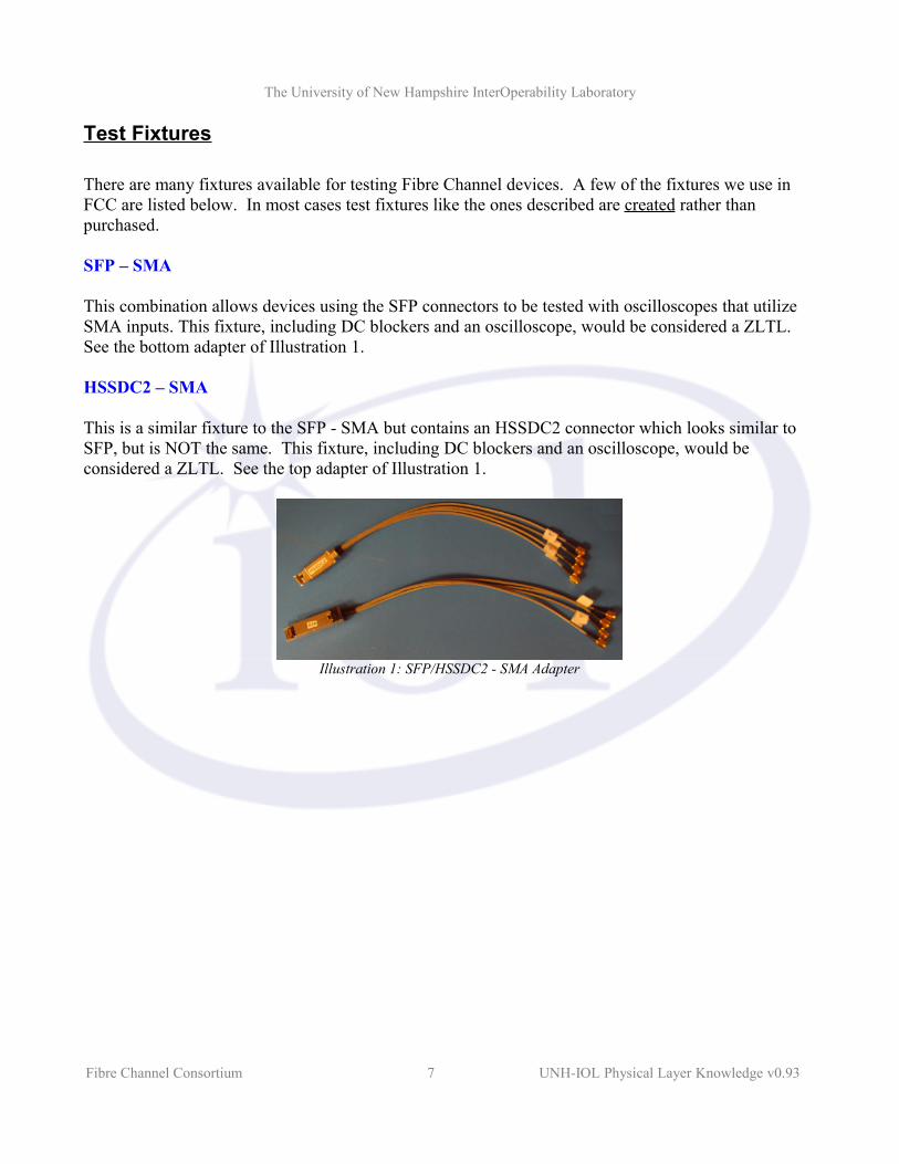
This combination allows devices using the SFP connectors to be tested with oscilloscopes that utilize SMA inputs. This fixture, including DC blockers and an oscilloscope, would be considered a ZLTL. See the bottom adapter of Illustration 1.

HSSDC2 – SMA

This is a similar fixture to the SFP - SMA but contains an HSSDC2 connector which looks similar to SFP, but is NOT the same. This fixture, including DC blockers and an oscilloscope, would be considered a ZLTL. See the top adapter of Illustration 1.


Illustration 1: SFP/HSSDC2 - SMA Adapter


SCA-2 (FC) – SMA

References: SFF-8045 - 2.3

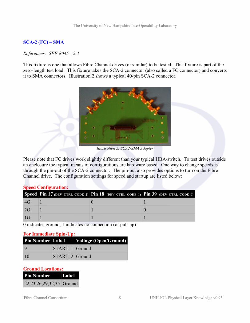
This fixture is one that allows Fibre Channel drives (or similar) to be tested. This fixture is part of the zero-length test load. This fixture takes the SCA-2 connector (also called a FC connector) and converts it to SMA connectors. Illustration 2 shows a typical 40-pin SCA-2 connector.

Please note that FC drives work slightly different than your typical HBA/switch. To test drives outside an enclosure the typical means of configurations are hardware based. One way to change speeds is through the pin-out of the SCA-2 connector. The pin-out also provides options to turn on the Fibre Channel drive. The configuration settings for speed and startup are listed below:

Speed Configuration:Speed Pin 17 (DEV_CTRL_CODE_2) Pin 18 (DEV_CTRL_CODE_1) Pin 39 (DEV_CTRL_CODE_0)

4G 1 0 12G 1 1 01G 1 1 10 indicates ground, 1 indicates no connection (or pull-up)

For Immediate Spin-Up:Pin Number Label Voltage (Open/Ground)9 START_1 Ground10 START_2 Ground

Ground Locations:Pin Number Label22,23,26,29,32,35 Ground


Illustration 2: SCA2-SMA Adapter


Test Patterns

References: T11 – MJSQ - Annex A

Test patterns:

D21.5

Purpose: When testing generic transmitter tests we use continuous D21.5 as it provides a continuous stream of 0/1 transitions. This more or less creates a time-domain signal that eliminates the effects caused by long lengths of 0s or 1s (signal doesn't have the nicety of being able to reach a well known steady-state). It also helps by eliminating the effects of pre-compensation. The standard defines this pattern specifically for Rise Time, Fall Time and Skew measurements.

Data Byte Name Bits HGF EDCBA (binary)

Current RD – abcdei fghj (binary)

Current RD + abcdei fgh (binary)

D21.5 101 10101 101010 1010 101010 1010

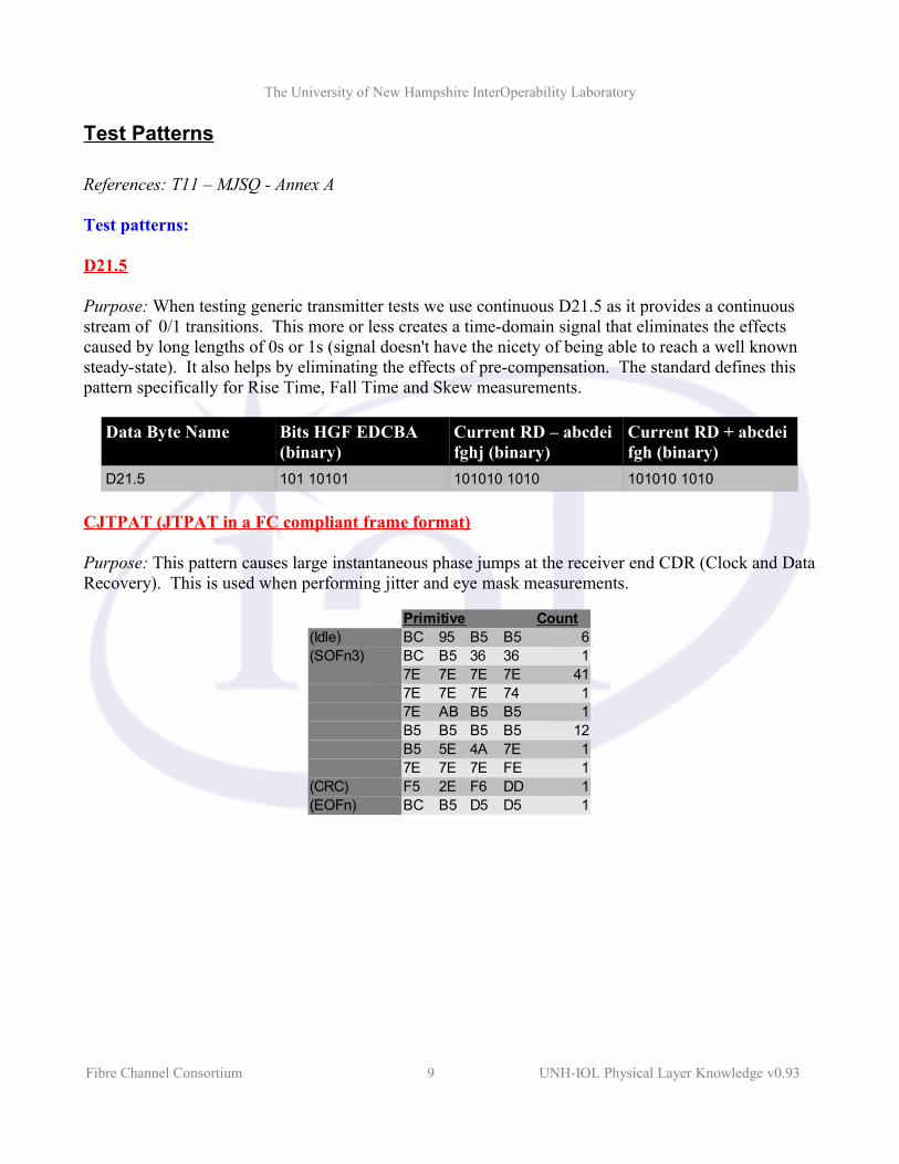
CJTPAT (JTPAT in a FC compliant frame format)

Purpose: This pattern causes large instantaneous phase jumps at the receiver end CDR (Clock and Data Recovery). This is used when performing jitter and eye mask measurements.


Primitive Count(Idle) BC 95 B5 B5 6(SOFn3) BC B5 36 36 1

7E 7E 7E 7E 417E 7E 7E 74 17E AB B5 B5 1B5 B5 B5 B5 12B5 5E 4A 7E 17E 7E 7E FE 1

(CRC) F5 2E F6 DD 1(EOFn) BC B5 D5 D5 1


CRPAT (RPAT in a FC compliant frame format)

Purpose: CRPAT is an important pattern while testing Return Loss as it provides a flat spectrum. This is used when performing jitter and eye mask measurements.

CSPAT (SPAT in a FC compliant frame format)

Purpose: This pattern introduces SSO (Simultaneous Switching Output) noise, from the power supply, through the transceiver. This is used when performing jitter and eye mask measurements.

How to get a device to transmit test patterns?

There are a few ways to get devices to transmit the necessary patterns.

1. For most devices that want electrical testing there is the low-level ability to have the device transmit the required patterns at the required speeds.

2. Another method would be to have the device enter a loop-back mode. At this point it is possible to transmit the patterns from a generator and the device should retransmit them. Before testing it must be understood where this loop-back is occurring. If the device loops back at the front end (before the SERDES), the testing would not be typical of how the device will act while in actual use. Care must be taken to ensure the loop-back is at least after the SERDES.

3. Another method is for loop devices that cannot be controlled in any of the other methods. In this case it is necessary to utilize the LPB primitive. This method entails bringing them through loop initialization and then transmitting a LPB primitive to them, thus putting them in a loop-back mode. Again, care must be taken as to how the device is performing loop-back.

4. The last method is for point-to-point devices. This method entails encapsulating the patterns in a FC ECHO frame. Care must then be taken to either eliminate the extra header/Idle



BE D7 23 47166B 8F B3 14

5E FB 35 59(CRC) EE 23 55 16 1(EOFn) BC B5 D5 D5 1


7F 7F 7F 7F 512(CRC) F1 96 DB 97 1

BC 95 D5 D5 1(EOFn)


information when taking measurements or ensure that it does not affect the patterns in a negative manner.



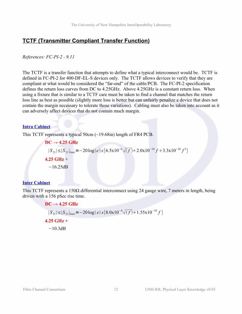
TCTF (Transmitter Compliant Transfer Function)

References: FC-PI-2 - 9.11

The TCTF is a transfer function that attempts to define what a typical interconnect would be. TCTF is defined in FC-PI-2 for 400-DF-EL-S devices only. The TCTF allows devices to verify that they are compliant at what would be considered the “far-end” of the cable/PCB. The FC-PI-2 specification defines the return loss curves from DC to 4.25GHz. Above 4.25GHz is a constant return loss. When using a fixture that is similar to a TCTF care must be taken to find a channel that matches the return loss line as best as possible (slightly more loss is better but can unfairly penalize a device that does not contain the margin necessary to tolerate those variations). Cabling must also be taken into account as it can adversely affect devices that do not contain much margin.

Intra CabinetThis TCTF represents a typical 50cm (~19.68in) length of FR4 PCB.

DC → 4.25 GHz

|S 21 |≤|S 21 |limit=−20 log e x [6.5x10−6 f 2.0x10−10 f 3.3x10−20 f 2]

4.25 GHz +−16.25dB

Inter CabinetThis TCTF represents a 150Ω differential interconnect using 24 gauge wire, 7 meters in length, being driven with a 156 pSec rise time.

DC → 4.25 GHz

|S 21 |≤|S 21 |limit=−20 log e x [8.0x10−6 f 1.55x10−10 f ]

4.25 GHz +−10.3dB



Below is an example of an Intracabinet TCTF (currently used by the UNH-IOL):

Below the return loss is plotted along side the ideal return loss specification lines. The return loss of the above setup has slightly more loss which is ok. The top line (black) is the specification and the bottom line (blue) is the Tyco backplane.


Illustration 3: Tyco Backplane (16 inch FR4 trace, 2 HMZD adapters, (4) 12" cabling)

Illustration 4: Tyco Backplane Return Loss (including cabling)


Eye Masks

References: FC-PI-2 – 9.3, 9.4, 9.6

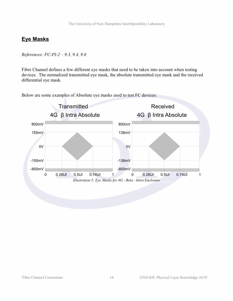
Fibre Channel defines a few different eye masks that need to be taken into account when testing devices. The normalized transmitted eye mask, the absolute transmitted eye mask and the received differential eye mask.

Below are some examples of Absolute eye masks used to test FC devices:


Illustration 5: Eye Masks for 4G - Beta - Intra Enclosure

4G β Intra Absolute 4G β Intra AbsoluteTransmitted Received

0V

0.26UI 0.5UI0 0.74UI 1

155mV

-155mV

800mV

-800mV

0V

0.26UI 0.5UI0 0.74UI 1

138mV

-138mV

800mV

-800mV





0V

300mV

-300mV

1000mV

-1000mV0.165UI 0.355UI0 0.645UI 0.835UI 1

0V

0.165UI 0.5UI0 0.835UI 1

200mV

-200mV

1000mV

-1000mV



0V

300mV

-300mV

1000mV

-1000mV0.115UI 0.305UI0 0.695UI 0.885UI 1

0V

0.115UI 0.5UI0 0.885UI 1

200mV

-200mV

1000mV

-1000mV


De-embedding

References: FC-PI-2 – Appendix B.3

Since FC connectors are different than test connectors, care must be taken to exclude all extra cabling/traces/connectors that can affect the measurement. FC-PI-2 has a section that discusses where to de-embed to but lacks any discussion on how to perform this. In this case we care most about de-embedding when performing return loss measurements. In most cases the de-embedding should be through the applicable fixture to the FC connector. For example: when using the zero length test load of the SCA-2 to SMA adapter for return loss testing, the cables of the VNA as well as the SMA and PCB up until the end of the SCA-2 connector needs to be de-embedded.

There are a few methods that are available to de-embed “properly”:1. Do not de-embed

a. This is only reasonable if the fixture is proven to be much “better” than what the DUT. This is a comparison that is tough to make, so we will replace “better” with “good”. Since “good” is not the easiest term to define we can reasonably assume that with good trace layout, good connectors and good return loss measurements that the fixture will be “good”. This assumption is only valid if the amount of return loss is insignificant enough to make the DUT fail. Keep in mind that devices on the edge of failing may be incorrectly failed due to the addition of the fixture (not an acceptable practice). In this case de-embedding must be done or another method to remove the fixture to prove the failure.

2. De-embed a. This can be accomplished, assuming custom hardware is available, to de-embed fixtures

with SCA-2 or SFP ends. (e.g. for SCA-2 connectors it is necessary to have a male connector that provides a short/open/load in order to calibrate the VNA). This is the ideal case and should always be used unless this is not feasible with current equipment.

3. Software de-embedding a. This is where the time-domain signal is observed (through TDR or VNA/IFFT) and the

fixture is removed from the signal and then the remaining signal is converted back to the frequency domain using the FFT operation. This is not an optimal method but can be used if true de-embedding is not feasible. This method may provide slightly better results than not de-embedding, assuming the software routine has been proven to provide robust results.



Transmitter TestsNominal Bit Rate

Fibre channel often refers to speeds of 1GFC, 2GFC, 4GFC, 8GFC, etc.. What this means is actually 1.0625GBd, 2.125 GBd, 4.25 GBd, 8.5 GBd, etc. This is the baud rate (symbols/sec). According to the FC-PI-2 standard 1 symbol is equivalent to 1 bit. In this case the “baud rate” is equivalent to the “bit rate”.

T is the period of the waveform. From the illustration we can see that the waveform contains 2 bits. A zero bit and a one bit. So for a 4.25GBd data rate the signal rate is 2.125GHz. This relationship holds true for the other rates as well.

When measuring signals it is important that enough harmonics are measured. For general purposes measuring out to 3 harmonics is ideal. However, care must be taken to not measure too many harmonics as this can introduce more noise into the system. The example seen in Illustration 9 shows that 6.375GHz is the 3rd harmonic. To measure this we use the Nyquist rate and determine from it that we need a sampling rate of at least 12.75G samples/sec. Exactly how much is too much is a tough thing to quantify, therefore it is a good idea to measure only slightly over the Nyquist rate.

2 x 6.375GHz=12.75G samplessec

Fibre Channel also specifies that this measurement must be taken over 200,000 transmitted bits.


Illustration 8: 1 Period of SignalT

Illustration 9: 4GFC Harmonics Example2.125 GHz 4.25 GHz 6.375 GHz

4GFC

3rd Harmonic

2nd Harmonic

1st Harmonic


Differential Output Voltage

With differential signaling a signal is transmitted on a TX+ line and the complement is transmitted on a TX- line (hence the + and -). The Differential Output Voltage (DOV) is then the subtraction of the TX- from the TX+. Then we have:

TX p−TX m=TX p−−TX p=2TX p

The benefit of this, and thus differential signaling is then easily shown:

[TX pNOISE]−[TX mNOISE ]=TX pNOISE−−TX p−NOISE=2TX p

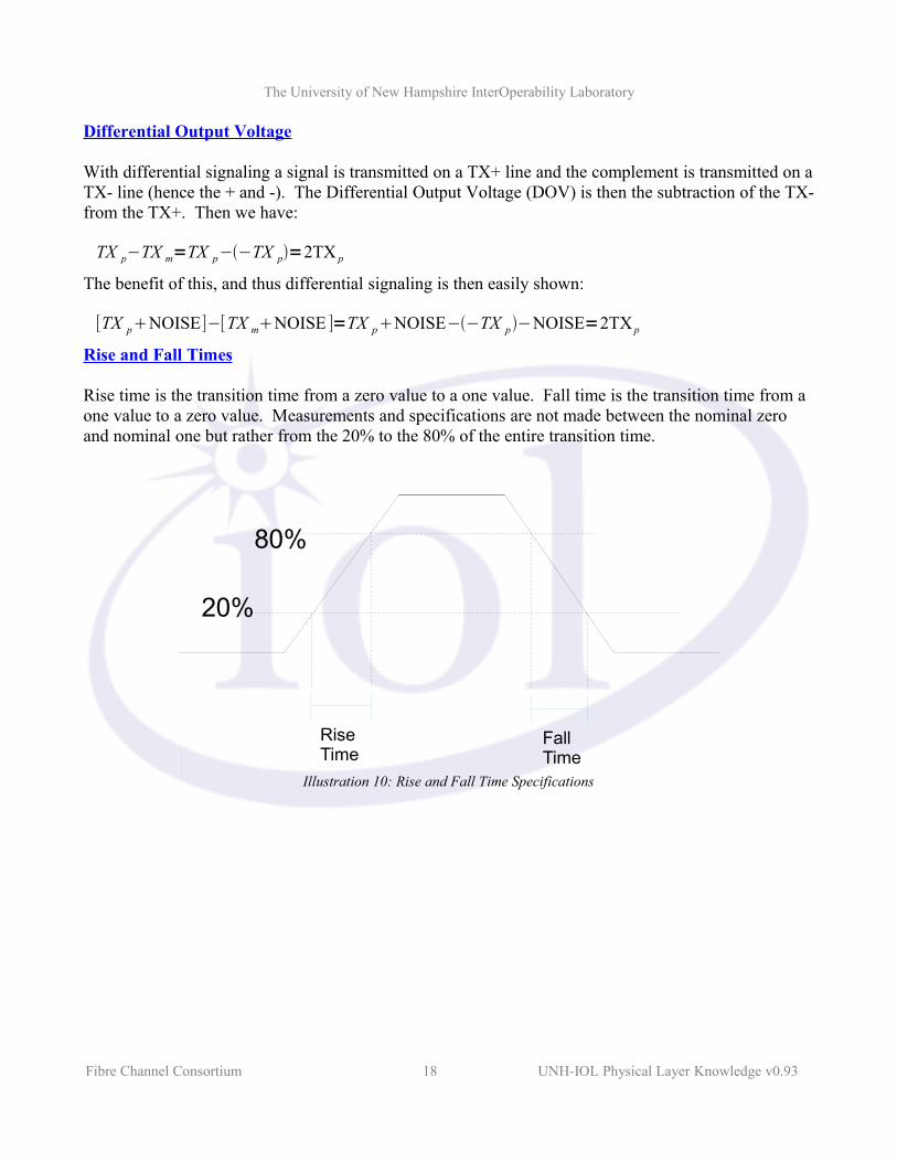
Rise and Fall Times

Rise time is the transition time from a zero value to a one value. Fall time is the transition time from a one value to a zero value. Measurements and specifications are not made between the nominal zero and nominal one but rather from the 20% to the 80% of the entire transition time.


Illustration 10: Rise and Fall Time Specifications

80%

20%

Rise Time

Fall Time


Transmitter Eye Mask

This test takes an eye of the transmitted signal over a period of time and compares it against an eye mask. This test utilizes 3 transmitted signals (patterns). CJTPAT, CRPAT and CSPAT are used to cause various transitions to occur to cause the output signal to be considered “worst case”. This is done to ensure that if a device can transmit the patterns without error that they are unlikely to encounter an eye mask issue during typical signaling.

Different types of devices have different types of eye masks. Earlier in the Eye Mask section there are a few illustrations where the data from the standard is shown next to an eye mask. Depending on the device a different mask will have to be compared with the signal. In general the signal must not violate the eye (enter the center region, leave the boundary regions).

Transmitter Jitter

This test measures the Peak-to-Peak Deterministic Jitter and the Peak-to-Peak Total Jitter. Various methods are used to measure jitter. A quick visualization of jitter can be done by looking at the crossing points of the signal in the Transmitter Eye Mask test.

Deterministic Jitter This is jitter that follows a predictable pattern.

Total Jitter This is the addition of Deterministic Jitter and Random Jitter.

Transmitter RMS Common Mode Voltage

This test is only applicable to 4GFC devices. This measurement takes the TX+ and adds it to the TX-. What this gives you is the common mode signal. Once you have a common mode signal you can then compute the RMS value over it and you will have the RMS Common Mode Voltage.

The generic formula is defined as:

1n∑i=1

n

V p , iV m ,i 2

| n = length of the signal | p = positive | m = minus|



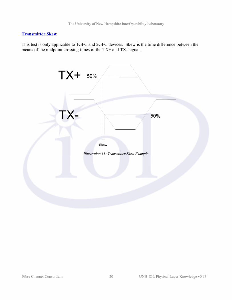
Transmitter Skew

This test is only applicable to 1GFC and 2GFC devices. Skew is the time difference between the means of the midpoint crossing times of the TX+ and TX- signal.


Illustration 11: Transmitter Skew Example

Skew

50%

50%

TX+

TX-


Return LossReferences: FC-PI-2 - Table 23

Generic Description

Return loss is a measure of the amount of signal that is reflected relative to a transmitted incident signal. When a signal is transmitted down any sort of transmission line there are certain impurities (e.g. capacitance and inductance) and discontinuities in the medium, connectors and/or specific PCB structuring (e.g. vias). These impurities cause impedance mismatches which cause part, or sometimes all, of the signal to reflect back towards the source. The smaller the mismatch the smaller the reflection.

In order to make these measurements there are two typical measurement devices. A Vector Network Analyzer (VNA) or a Time Domain Reflectometer (TDR).

VNAA VNA measures return loss in the frequency domain (power versus frequency). The VNA sends sinusoidal signals at a specified frequency and then observes the reflected signal at that same frequency. As it is impossible to measure exactly one frequency, a very small range is filtered out and measured. The VNA eventually sweeps over the entire frequency range taking measurements as it goes. When taking measurements in this case it is important to have as flat a spectrum as possible. If the spectrum includes spikes at certain frequencies then the VNA will take measurements that include this spike; thus causing possible errors in measurement. Fibre Channel has the CRPAT pattern that provides this flat spectrum.

TDRA TDR measures return loss in the time domain (voltage versus time). The TDR works by transmitting a short pulse down the medium and measures the amount of signal that is reflected back. The time to receive the signal back is noted and plotted based upon the various times and amount of energy reflected. A benefit of this type of measurement is being able to see exactly where the reflected energy occurred and being able to calculate the exact distance to this point.

The basic formula for calculating return loss is as follows:

RL dB=−20log10V r

V i *A smaller reflected signal results in a higher return loss. Ideally you do not want any reflected signal, thus you want a higher return loss.



When return loss is measured, it is typical to take the measurements with S-Parameters. S-Parameters are a way to determine what a device acts like based upon the network theory. With differential signaling, two-port network theory applies. Following the generic convention SXY means the test signal was transmitted on Y and observed on X.

S-Parameters that we are interested in

SDD11 is defined as the differential mode return loss for port 1. This tells us what the differential mode reflection back to the source is when a differential mode signal is applied. i.e. the ratio between the two differential mode signals.

SCC11 is defined as the common mode return loss for port 1. This tells us what the common mode reflection back to the source is when a common mode signal is applied. i.e. the ratio between the two common mode signals.

SDD22 and SCC22 are both the same as SDD11 and SCC11 but on port 2 of the VNA. UNH-IOL typically connects port 2 to the Transmitter and port 1 to the Receiver.

Fibre Channel Specifics

In FC devices it is a good idea to use a VNA to measure return loss. The return loss curves are described in terms of gain versus frequency. Since VNAs measure in the frequency domain it is natural to take the measurement using this device. When measuring signals on a VNA it is important to keep the flat spectrum. Thus it is common to have the DUT transmit CRPAT while the VNA is taking measurements.

Measurements are just as valid with a TDR.



S-Parameter Compliance Limit Lines

The above Illustrations are plots of the limit lines for 4G Beta Transmit devices. The differential return loss limit lines are seen to require a greater amount of loss when compared to the common mode case. These measurements are made from 50MHz to 3.2GHz


Illustration 13: Return Loss for Beta T Devices (SCC22)

0 . 5 1 1 . 5 2 2 . 5 3 3 . 5 4

0

2

4

6

8

1 0

1 2

Ret

urn

Loss

(dB

)

F r e q u e n c y ( G H z )

R e t u r n L o s s P l o t f o r B e t aT

( S C C 2 2 )

Illustration 12: Return Loss for Beta T Devices (SDD22, SDD11)

0 . 5 1 1 . 5 2 2 . 5 3 3 . 5 4

0

2

4

6

8

1 0

1 2

Ret

urn

Loss

(dB

)

F r e q u e n c y ( G H z )

R e t u r n L o s s P l o t f o r B e t aT

( S D D 2 2 , S D D 1 1 )

unh-iol physical layer knowledge document · unh-iol physical layer knowledge document university...

Documents