Unemployment Risk and Consumption: Can the

Buffer Stock Saving Behavior Explain the Japanese

Experience?∗

Masayuki Keida†, Takashi Unayama‡

and Katsunori Yamada§

Abstract

This paper shows that the drop of the aggregate propensity to

consume (APC) in Japan during the lost decade is attributable to

increase of income risks, mainly due to the rise in the unemployment

rate. In order to assess impacts of income risks numerically, we use

a buffer stock saving model that deals with transition dynamics of

wealth distribution. Our simulation results well capture the evolution

of the APC during the 1990s, which suggests not only the drop of the

APC can be explained with the buffer stock saving behavior, but also

it would be transit.

Keywords: Income Risk, Japanese Household Consumption, Pre-

cautionary Saving.

JEL classifications: E21, D91, E27

∗We are grateful to Christopher Carroll, Shin-ichi Fukuda, Michael Haliassos, Akihisa

Shibata, and seminar participants at the University of Cyprus for their helpful comments

and discussions.†Graduate School of Economics, University of Tokyo‡Corresponding Author: Kyoto Institute of Economic Research, Kyoto University:

Yoshida-Hommachi, Sakyo-ku, Kyoto city, JAPAN. E-mail: unayama@kier.kyoto-u.ac.jp§Graduate School of Economics, Kyoto University

1

1 Introduction

This paper shows, using a numerical method, that precautionary saving

motives can explain the fall of aggregate propensity to consume (APC) in

Japan during the lost decade; that is, the long-continued drop of the APC is

attributable to the increase of income risks during the 1990s. Unlike previous

studies, we focus on dynamics of wealth distribution which is driven by the

optimal consumption-saving decision.

Japan has long been in slump since the early 1990s, which is referred

to as the lost decade. The Japanese economy of this era has two particular

features; serious drop of the APC and unprecedented rise of unemployment

rate. To analyze the relationship between consumption and income risks,

the precautionary saving theory has been applied in previous studies (see

Ogawa, 1991; Nakagawa 1998; Murata, 2003; and Doi, 2004 for Japanese

economy).

Among precautionary saving models, one of the most important models

is the buffer stock saving model pioneered by Deaton (1991) and Carroll

(1992). They show that if households face higher income risks, they would

save more in order to prepare for unfortunate realization of their income

states. Moreover, the buffer stock savers would have a target wealth such

that, if wealth is below the target, households consume less and accumulate

wealth, while if wealth is above the target, households dissave. Carroll (1992;

1994; 1997) emphasize that the target wealth increase when income risks

become higher, which implies that households facing higher income risks

have more saving stocks. Some empirical studies support this implication

(for example, Carroll and Samwick, 1998; Carroll, Dynan and Krane, 1999;

and for Japanese evidence, Bessho and Tobita, 2004).

It is, however, well known in the literature that once households achieve

the target wealth, consumption out of flow income hardly depends on the

degree of income risks. In other words, the APC is affected by income risks

only immediately after the degree of risks changed, that is, while being on

the transition towards some stable level of the APC. This suggests that we

should consider the transition dynamics of wealth level in explaining the

2

long-continued drop of the APC as seen in Japan.1

Our framework basically follows Carroll’s buffer stock saving model.

Firstly, we set up a standard dynamic utility maximization problem in which

households face income risks. Then, we calibrate the model with Japanese

aggregate time series data for 1990-2002, and obtain the consumption func-

tion in terms of “cash on hand” for each year. With the consumption func-

tion and the dynamics of wealth distribution derived from the optimal be-

havior, we calculate the path of aggregate consumption.

Our calculation extracts two main conclusions. Firstly, it turns out that

the consumption function shifts downwards during the 1990s, which implies

that the consumption level decreases for any wealth level, and that the target

wealth would become higher. In particular, the calculated target wealth

increases distinguishably for 1997-1999 when the unemployment rate rose

sharply. Such changes of the target wealth induce households to consume

less and save more in order to achieve the new target, while if households

reach at the new target, the APC would be almost same as the previous

level. Secondly, the simulated path of the APC well captured the real data of

Japan. This result suggests that the behavior of households on the transition

towards the new target can explain the Japanese consumption behavior in

the 1990s.

In addition to these results, there is an interesting yet unintuitive impli-

cation. By the assumption of our calculation, the fall of the APC during the

lost decade would be transitory, and hence, consumption can be expected

to recover without any improvements of economic situations. This impli-

cation seems to be consistent with the very recent recovery of household

consumption, whereas the unemployment rate continues to stay relatively

high level.

This paper constructed as follows. Section 2 set up the model and defines

some important concepts. In particular, the definitions of the long-run and

the short-run propensity to consume are significant in our analysis. Section

3 discusses the data construction. Section 4 presents the calculation results

1Murata (2003) and Doi (2004) empirically investigate the effects of income risks on

household saving rate, but theoretical backgrounds of their estimates are not clear.

3

and discusses some implications. Section 5 concludes.

2 The Model

The framework of analysis follows Carroll’s buffer stock saving model. Sup-

pose that a household solves a dynamic utility maximization problem. There

is no uncertainty with regard to the interest rate and no credit constraint.

Households, however, earn wage income that varies stochastically.

The maximization problem at time t is

maxCt

u(Ct) +

∞∑j=t+1

βj−tEtu(Cj)

, (1)

subject to

At = RAt−1 + Wt − Ct, (2)

where u, β, At, Ct, and Wt is the instantaneous utility function, the dis-

count rate, asset holding at the end of period t, consumption, and wage,

respectively. R is the constant gross interest rate that is one plus the real

interest rate, r.

In our model, the wage income is subject to transit shocks while we

omit the permanent shocks since there is only few evidence about distinction

between permanent and transitory income shocks for the Japanese household

income profile. By decomposing the realization of income into two factors,

we obtain,

Wt = Ytεt = GYt−1εt, (3)

where Yt is the permanent income that deterministically grows at constant

rate, G and εt is the transitory income shock.

The transitory shock, εt, is denoted by households’ employment status.

Suppose there are three states; employed as a higher wage worker, employed

as a lower wage worker, and an unemployed. When a household is employed

as a higher wage (lower wage) worker, the wage is the permanent income

4

multiplied with wH (wL), while an unemployed household earns no income.

In addition, we assume that εt follows the i.i.d. process; then, the process is

εt =

0 with probability µt

wL with probability (1 − µt)pL

wH with probability (1 − µt)(1 − pL).

(4)

These assumptions imply that the probability of job-loss, µt, is equal to the

unemployment rate and pL is the share of the lower wage workers among

employees.

Following previous studies, we define the cash on hand, Xt, as the sum

of the beginning-of-period wealth and the wage income (that is, Xt ≡RAt−1 + Wt). In order to obtain numerical solutions, the instantaneous

utility function is assumed to be of the CRRA and all variables are divided

by the level of permanent income.2 Then, the problem can be rewritten in

the recursive form as,

v(xt) = maxct

{u(ct) + βG1−ρEtv(xt+1)

}, (5)

subject to

xt+1 = (R/G)(xt − ct) + εt+1,

where the lower letters denote the ratio to the permanent income, Yt.

Carroll and Kimball (1996) show that the optimal consumption at time

t depends only on the cash-on-hand at time t in this framework with a

given income process. Accordingly, we can obtain the following consumption

function of households;

ct = c(xt). (6)

In the literature, it is well established that if households follow the buffer

stock saving behavior, they have the target wealth such that, if wealth is

below the target, they consume less to accumulate wealth, while if wealth

2In our calibration, households are found to be impatient throughout the era of the

simulation in the sense that they satisfy the condition of (Rβ)1/ρ < G. This means the

existence of buffer stock motivation. For the analytical proof of this argument, see Carroll

(2002).

5

is above the target, they dissave. The target wealth in our model can be

obtained as the fixed point of the budget constraint as

a∗ =G

G − R

{Et(wt+1) − c

(R

Ga∗ + Et(wt+1)

)}, (7)

where a∗ is the target wealth.

In principle, the wealth would stably converge toward the target wealth;

however, since there is the income shock generated by εt, the wealth of each

household fluctuate around the target level such that in the economy, the

level of wealth has a non-degenerate distribution. Carroll (1992; 1994; 1997)

find by simulation a property about the wealth distribution that there is the

steady-state wealth distribution that emerges after sufficiently many periods

and it depends only on the consumption function.3

From the optimal consumption behavior for each household obtained

above, we consider the aggregate consumption and propensity to consume.

Suppose there is a distribution of wealth at time t, Ft(a), then the distribu-

tion of the cash-on-hand can be easily obtained since the wage distribution

is independent of Ft(a). Thus, we can calculate aggregate consumption by

evaluating the consumption function at each cash-on-hand level and sum-

ming up them with the weights from the distribution of x. Accordingly, the

aggregate consumption, ACt, is a functional of c(x) and Ft(a):

ACt = AC(c(x), Ft(a)). (8)

Using the budget constraint of each individual household, we can derive

the distribution of wealth for the beginning of the next period, Ft+1(a),

which implies that the consumption function determines the evolution of

the distribution of wealth.

In our framework, therefore, propensity to consume can be calculated as

follows:

SPCt =AC(c(x), Ft(a))

(R/G − 1)∫

adFt(a) + E(wt), (9)

where the numerator is the aggregate consumption defined above. The de-

nominator is the aggregate income, that is, the sum of capital income from3For analytical proof of this argument, see Carroll (2002).

6

the wealth and the labor income, wt. We refer to this propensity to con-

sume as the short-run propensity to consume (SPC) since the distribution

of wealth that we use for this calculation is not the steady state one.

In addition to the SPC, it will be useful to define the propensity to con-

sume that emerges when the distribution of the wealth converges toward the

steady-state one. We refer to this propensity to consume as the long-run

propensity to consume (LPC). Since the steady-state distribution depends

only on the consumption function, the LPC is also determined by the con-

sumption function. The LPC is,

LPCt =AC(c(x), F ∗(a))

(R/G − 1)∫

adF ∗(a) + E(wt), (10)

where F ∗(a) is the steady-state distribution of wealth. Since the difference

between the SPC and the LPC comes from the distribution of wealth, the

SPC will converge to the LPC if the consumption function is fixed.

3 Data

To calibrate the model to the Japanese economy during the lost decade, we

construct the parameters that appear in the model: unemployment rate µ;

real interest rate, r; real income growth factor, G; lower wage, wL; higher

wage wH ; and probability to be lower wage employee, pL, as well as the

aggregate propensity to consume.

Since the seminal paper of Deaton and Paxson (1994), many studies at-

tribute income variation to various heterogeneous factors across households

such as age, age cohort, education, and types of jobs (See Storesletten,

Telmer and Yaron, 2004a; 2004b; and Guvenen, 2004); and thus, income

risks that individual households face should be described with micro data.

However, we construct parameters from Japanese aggregate time series data

because of limited availability of Japanese household survey data.4 Since

we should use aggregate data, all households have been assumed to face the

4Ohtake and Saito (1998) provides some evidence about income variation from micro

data following Deaton and Paxson (1994), nevertheless information has still been limited.

7

same income risks in the model regardless of demographic and/or socioeco-

nomic factors.5

Firstly, we examine the APC in Japan. Figure 1 presents the APC

for the Japanese households in the 1990s, which is defined as consumption

expenditure divided by disposable income, and this is our goal that will

be explained using the model. We use the data from the Japanese Family

Income and Expenditure Survey (JFIES), while it is well known that the

saving rates from the JFIES and the SNA have moved differently.6 Figure 1

shows that the APC decreases during the decade, while it started to increase

after 1999, even though the Japanese economy as a whole might not escape

the slump.

Among dependent variables, the most important variable is the unem-

ployment rate since the buffer stock saving literature emphasizes that unem-

ployment (zero income state) seriously affects household consumption.7 We

can obtain the unemployment rate from the Labor Force Survey, and the

data for the 1990s is presented in Figure 2. The unemployment rate sharply

increases to over 5% after 1993, while it stably ranges from 2% to 3% before

the 1990s. In particular, the rise during 1997 to 1999 is distinguishable.

The factor of R/G is another important dependent variable. The real

interest rate, r, is defined as the Government Bond rate minus the inflation

rate of the Consumer Price Index (CPI), while the real income growth rate

is defined as change rate of the disposable income deflated by the CPI. Since

the interest rate and the inflation rate decrease in almost parallel, the real

interest rate is relatively stable during the decade.8 On the other hand, the

5In this sense, households are substantially homogenous even though the realizations of

employment status are heterogeneous. Heterogeneity stems only from the level of wealth.6Throughout the 1990s, the saving rate obtained from the SNA data does not show

such drops as in Figure 1, and the large part of this gap can be explained with the

coverage of the two statistics. The JFIES data cover households whose household head is

a wage earner that faces serious income risks. Therefore, we believe the JFIES would be

more relevant for our purpose, even though the SNA data is a more relevant statistical

indicator of macro consumption. For more discussion, see Ueda and Ohno (1993) and

Iwamoto, Oazaki, Maekawa (1995).7See, for example, Carroll (1992).8We subtract 1.5% from the inflation rate at 1997 in order to adjust the revise of

8

income growth rate is negative after 1998 when the financial crisis becomes

serious. Accordingly, R/G has a slightly increasing trend during the decade.

Since the higher R/G may shift downwards the consumption function, the

consumption level could be decreased by this change in R/G.

wL, wH and pL are not available directly from the data. We construct

these parameters using the average, the 20 percentile, and the 80 percentile

of yearly income of households from the JFIES. We regard the ratio of the

20 percentile to the average as the lower wage and that of 80 percentile as

the higher one. Then, the probability to become a lower wage employee is

set such that the expected income conditional on being employed equals to

unity. Finally, we multiply them with the real income, which is normalized to

be unity at 1990. These three parameters represent wage inequality among

employees that may generate wage risks in addition to the unemployment

risk. The calculated data indicates the inequality in Japan becomes larger

during the 1990s. This implies that households face higher income risks in

the 1990s. 9 However, it should be noted the heterogeneity of income risks

among different types of households is not considered here. By this omission

we may under- or over- estimate the income risks.10

Finally, there are two parameters in the model, the discount factor, β and

the elasticity of intertemporal substitution, ρ. They are quite controversial

parameters and difficult to give specific values.11 Here, we set them as

(β, ρ) = (.9, 5), which is very close to the calculation in Carroll (1992).12

consumption tax rate.9Discussion of wealth inequality in Japan is highly controversial. See, for example,

Ishikawa (1994) and Tachibanaki (1996).10Ohtake and Saito (1998) show that the log-income variance in Japan depends on age

and age cohort, and is ranged from 0.15 to 0.5, while our value is about 0.3.11Carroll (2001) argues that the usual estimation of the elasticity of intertemporal sub-

stitution may be biased.12Carroll (1992) uses the parameter values of (β, ρ) = (.9, 3) as the baseline and varies

within some reasonable range.

9

4 Results

4.1 Consumption Function and the Target Wealth

Using the aggregate data described above, we derive the consumption func-

tion in terms of the cash-on-hand, (6), for each year. Figure 3 presents the

consumption function for 1990, 1995 and 2000, which clearly shows the con-

sumption schedule shifts downwards at any cash-on-hand level. Hence, the

aggregate consumption decreases if the distribution of the cash-on-hand is

fixed.

This downward shift implies that the target wealth become higher, thus

we also calculate the target wealth for each year using the consumption

functions obtained above. The higher line in Figure 4 presents the time

path of the target wealth. The line shows that the target wealth became

higher along with the unemployment rate. This change of target wealth

level leads to the transit change of the APC.

As noted above, possibility of being zero income state has distinguished

effects on household consumption. In order to clarify the impact of unem-

ployment rate, we calculate the target wealth for an economy in which we

keep the unemployment rate fixed at the level of 1990 and other parameters

are drown from the data. The result is presented with the lower line in

Figure 4. Although the parameters are same in the two calculations except

for unemployment rate, the two lines move quite differently. That is, if the

unemployment rate was kept constant, the target wealth would not increase

so sharply. This suggests that the large part of changes in the target wealth

would be attributable to the increase of the unemployment rate.

In addition to this analysis, there is another way to clarify the importance

of changes in the unemployment rate. When we investigate the consump-

tion function, we know the fall of consumption between 1990 and 2000 is

calculated as 8.25%, evaluating at the target wealth for 1990. However, if

the unemployment rate does not change during the 1990s, the consumption

would rather increase by 1.29%; that is, the increase in the unemployment

rate causes the drop of consumption by 9.54%.

From these analyses we can conclude that increases of income risks dur-

10

ing the 1990s affect the individual consumption behavior seriously. Next, we

have to aggregate these individual effects to evaluate the aggregate effects

on the APC.

4.2 The LPC and the SPC

As discussed above, the distribution of the wealth is required to assess im-

pacts of changes on the aggregate consumption. However, if we use some

statistics about assets of households, we would have some difficulties such

as domain of assets and/or valuation of real assets. Moreover, it is well

known that the distribution of wealth is seriously affected by demographic

structure due to the life cycle saving motive and the bequest motive, which

is not explicitly analyzed in our model. Therefore, instead of using actual

statistics about household assets, we assume that the wealth distribution at

the initial year of 1990 is the steady state distribution. This assumption

seems relevant since the economic situation was relatively stable for several

years before 1990.13

Here, we obtain the SPC and the LPC as follows. Since the evolution of

wealth distribution can be calculated with iterative uses of the consumption

functions for each year, the SPC defined with (9) can also be calculated when

the initial wealth distribution is given. On the other hand, it is possible to

calculate the steady-state distribution of wealth for each year, using the

corresponding consumption function. Accordingly, the LPC defined with

(10) can also be obtained, and it is dependent on not the dynamics of wealth

distribution but on the steady-state distribution for each year.

The broken line in Figure 5 shows the result for the LPC. As it can be

seen from the figure, the LPC is almost constant. This outcome is consistent

with theory that the APC is almost independent of income risks after the

wealth distribution converges to steady state one; although the consumption

function shifts downward as shown in Figure 3, the wealth distribution shift

rightward, which cancel the drops of consumption for every level of cash-on-

hand.

13We also calculate the steady state distributions for the year 1988, 1989 and 1991, and

obtain similar results reported here.

11

Our long-run implication above is consistent with Bessho and Tobita

(2004), who show using a cross sectional data that a household that faces

higher income risks has more stocks of savings in Japan as well as in the US.14

However, although it is a plausible test of the buffer stock saving theory, it

cannot explain a fall of the APC since the result of the LPC suggests that

consumption behavior is not sensitive to the changes of income risks in the

long-run.

In the short-run, on the other hand, changes of income risks do affect the

consumption behavior. The solid line in Figure 5 presents the result of the

SPC. The SPC traces the APC from the data which is presented with the

dotted line. This implies that, during the 1990s, effects of the downward shift

of consumption function dominates the effects of wealth accumulation. That

is, the target wealth increases too fast for agents to fill up the gap between

the previous target level of wealth and new one. It will be noteworthy that

the SPC can be obtained only when we consider the dynamics of wealth

distribution.

These results in the SPC and the LPC suggest not only that the fall

of propensity to consume would be caused by the increase of income risks

but also that it would be transitory. The latter implication, in particular, is

interesting yet unintuitive. Since it is transitory, it would be expected that

the propensity to consume could recover even without any improvements

of economic situation. The discrepancy between the implication and the

intuitive definition of transitory we are facing is that the APC has stayed

at lower level more than ten years. Furthermore, Carroll (1992; 1994; 1997)

point out that the convergence toward the steady state distribution is very

fast.15

However, the relationship between the model assumption and the con-

structed data would explain the discrepancy. While households regard the

parameters as constant over time in the model, the data for the parameters

14See, for US evidence, Carroll and Samwick (1997) and Carroll, Dynan, and Krane

(1999).15He concludes that usually it is not necessary to consider the SPC due to this fast

convergence.

12

are constructed for each year. Since the actual values are different for each

year, our model implicitly assumes that expectation of households has been

different from the realization throughout the 1990s. In other words, we im-

plicitly assume that the expectation of households has been underestimating

the worsening of economic situation during the lost decade.

It may seem an unusual assumption but there are some evidences indi-

cating that households failed to predict the future situation in the 1990s.

Doi (2004), who constructs a measure for income risks from the survey data,

shows that households underestimated the seriousness of recession and rec-

ognized the increase of income risks only after the unemployment rate has

risen significantly in late 1990s.16 That is, the changes of income risks were

not predictable at the year of 1990. If household could predict the worse

economic situation at 1990, the propensity to consume would be higher in

the 2000, even though the fall of the APC might be lager than the actual in

the early 1990s.

We will close this section by mentioning about the recovery of the APC.

Although recent recover of APC in data seems to be implied by our sim-

ulation, it is future interesting to know when the APC will recover to the

level of 1990. Hence, we simulate the APC in future with parameter values

fixed at 2002 level and our simulation, which indicates that it take about

ten years. This seems rather long as Carroll (1992) predicted that it might

be shorter. However, if we simulate with parameters of 2003, we find that

the path of recovery in the APC is more drastic and coincides with the

prediction by Carroll.

5 Conclusion

Many researchers focused on the relationship between consumption and in-

come risks with precautionary saving models, and empirical evidence has

shown that the buffer stock saving model appears to be consistent with the

Japanese household consumption behavior.

However, previous studies for the Japanese economy in the line of Deaton

16Nakagawa (1998) also provided similar results.

13

(1991) and Carroll (1992) care only about the long-run implications of the-

ory, and so they are not suited for explaining the drop of the APC. On

the other hand, our quantitative analysis clearly illustrates that the buffer

stock saving behavior causes the fall of the APC. In particular, the evolution

of the wealth distribution plays the central role in our analysis. As far as

we know, this is the first application for Japanese economy with explicitly

considering for the transition dynamics of wealth distribution.

One of the most interesting implications of our results is that the fall

of propensity to consume is a transitory phenomenon even though it has

continued more than ten years. This discrepancy between the implication

and the intuitive definition of transitory would be explained by the fact that

the households might underestimate the deterioration of economic situation

at the starting point of the slump. The repeated revision of the expectation

caused the prolonged transition toward the steady state.

For future research, it would be required to utilize micro data to allow

the heterogeneity of income profiles across households. Furthermore, the

model might be changed to finite horizon framework such that the model

includes the life cycle implications.

14

References

[1] Bessho, Shun-ichiro and Eiko Tobita (forthcoming). “Unemployment

risk and buffer-stock saving: An empirical investigation in Japan.”

Journal of Japanese and International Economics.

[2] Carroll, Christopher D. (1992). “The Buffer-Stock Theory of Saving:

Some Macroeconomic Evidence.” Brookings Papers on Economic Ac-

tivity, vol. 1992 No. 2, pp. 61-135.

[3] Carroll, Christopher D. (1994). “How Does Future Income Affect Cur-

rent Consumption?” Quarterly Journal of Economics, vol. 109 No. 1,

pp. 111-148.

[4] Carroll, Christopher D. (1997). “Buffer-stock Saving and the Life Cy-

cle/Permanent Income Hypothesis,” Quarterly Journal of Economics,

vol. 112, pp. 1-55.

[5] Carroll, Christopher D. (2000). “Requiem for the Representative Con-

sumer? Aggregate Impliations of Microeconomic Consumer Behavior”.

American Economic Review, 90(2), pp. 110 - 115.

[6] Carroll, Christopher D. (2001a). “Death to the Log-Linearized Con-

sumption Euler Equation! (And Very Poor Health to the Second Order

Approximation)”, Advances in Macroeconomics, vol. 1, Article 6.

[7] Carroll, Christopher D. (2001b). “Precautionary Saving and the

Marginal Propensity to Consume out of Permanent Income”, NBER

working paper. 8223.

[8] Carroll, Christopher D. (2002). “Theoretical Foundation of Buffer Stock

Saving”, manuscript.

[9] Carroll, Christopher D., Karen E. Dynan, and Spencer S. Krane

(1999). “Unemployment Risk and Precautionary Wealth : Evidence

from Households’ Balance Sheets, Finance and Economics Discussion

Series. No. 1999-15, Federal Reserve Board.

15

[10] Carroll, Christopher D., and Miles S. Kimball (1996). “On the Concav-

ity of the Consumption Function”, Econometrica, 64(4), pp. 981-992.

[11] Carroll, Christopher D., and Andrew Samwick (1998). “How important

is precautionary saving?”, Review of Economics and Statistics, vol. 80,

pp. 410-19.

[12] Deaton, Angus S. (1991). “Saving and Liquidity Constraints,” Econo-

metrica, 59, pp. 1221 - 1248.

[13] Doi, Takero (2004). “Increase in Saving Rate and Precautionary Saving

Motive in Japan.” In Hidehiko Ishihara and Takero Doi Consumption

and Saving Behavior of the Japanese in 1990: Theoretical Results and

Empirical Studies of Precautionary Saving Motive (Keizai Bunseki (The

Economic Analysis). No. 17, (In Japanese).

[14] Ishikawa, Tsuneo (Ed.) (1994). Income and Wealth Distribution in

Japan (Nihon no Syotoku to Tomi) University of Tokyo Press: Tokyo.

(In Japanese)

[15] Iwamoto, Yasushi, Tetsu Ozaki, and Hirotaka Maekawa, (1995). “On

discrepancy of saving rates between the JFIES and the SNA data (I).

(In Japanese)” Financial Review vol. 36 pp. 51-82.

[16] Guvenen, Fatih (2004). “Learning Your Earning: Are Labor Income

Shocks Really Very Persistent.” Presented at NBER Summer Institute

2004.

[17] Murata, Keiko (2003). “Precautionary Saving and Income Uncertainty:

Evidence from Japanese Micro Data.” Monetary and Economic Studies,

vol. 21, pp. 21-52.

[18] Nakagawa, Shinobu (1998). “Consumption Behavior under Uncer-

tainty.” Bank of Japan Working Paper Series 98-6 (In Japanese).

[19] Ogawa, Kazuo (1991). “ Income risks and Precautionary Saving.” Keiza

Kenkyu, vol.42, pp. 139-152. (In Japanese)

16

[20] Storesletten, Kjetil, Chris Telmer and Amir Yaron (2004a) “Consump-

tion and Risk Sharing over the Life Cycle.” Journal of Monetary Eco-

nomics vol. 51, pp. 609-633.

[21] Storesletten, Kjetil, Chris Telmer and Amir Yaron (2004b) “Cyclical

Dynamics in Idiosyncratic Labor Market Risk.” Journal of Political

Economy vol. 112, pp. 695-717

[22] Tachibanaki, Toshiaki (1994). Economical Inequality in Japan (Nihon

no Keizai Kakusa) Iwanami Shoten: Tokyo. (In Japanese)

[23] Ueda, Kazuo and Masatomo Ohno (1993). “Puzzles in household sav-

ing rate: discrepancy between the SNA and consumer survey data (In

Japanese).” Kin-yu Kenkyu vol. 12, pp. 127-145.

17

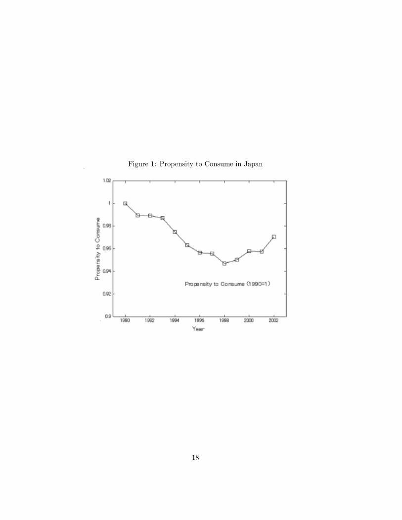
Figure 1: Propensity to Consume in Japan

18

Figure 2: Unemployment In Japan

19

Figure 3: Policy Function

20

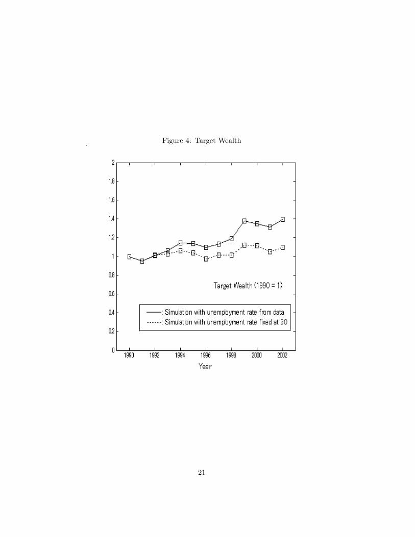
Figure 4: Target Wealth

21

Figure 5: Simulation Results and Data

22