underwater eit follow-on project final reportunderwater eit follow-on project final report . neptec...
TRANSCRIPT

Defence Research and Recherche et développement Development Canada pour la défense Canada
Underwater EIT Follow-on Project Final Report
Neptec Design Group Ltd. Contract Scientific Authority: J.E. McFee, DRDC Suffield
Defence R&D Canada
Contract Report
DRDC Suffield CR 2009-075
January 2009
The scientific or technical validity of this Contract Report is entirely the responsibility of the contractor and the contents do not necessarily have the approval or endorsement of Defence R&D Canada.

Underwater EIT Follow-on Project Final Report
Neptec Design Group Ltd. 302 Legget Drive Kanata ON K2K 1Y5 Contract Number: W7702-07R159/001/EDM Contract Scientific Authority: J.E. McFee (403-544-4739) The scientific or technical validity of this Contract Report is entirely the responsibility of the contractor and the contents do not necessarily have the approval or endorsement of Defence R&D Canada.
Defence R&D Canada – Suffield Contract Report DRDC Suffield CR 2009-075 January 2009

© Her Majesty the Queen as represented by the Minister of National Defence, 2009
© Sa majesté la reine, représentée par le ministre de la Défense nationale, 2009

302 Legget Drive, Kanata, Ontario Canada K2K 1Y5 Tel.: (613) 599-7602 Fax: (613) 599-7604
© HER MAJESTY THE QUEEN IN RIGHT OF CANADA (2009
NDG009087 Rev 1 Jan 7th 2009
UNDERWATER EIT FOLLOW-ON PROJECT
FINAL REPORT
CONTRACT NO.: W7702-07r159/001/EDM
Prepared for:
Dr. John McFee DRDC Suffield

NDG009087 Rev 1 EIT Follow-on Investigation Final Report January 7, 2009 Contract No: W7702-07r159/001/EDM
© HER MAJESTY THE QUEEN IN RIGHT OF CANADA (2009) ii
DOCUMENT APPROVAL RECORD
DOCUMENT NDG009087 Title: Underwater EIT Follow-on Project Final Report
Prepared By: Date: Jan. 2009
Author: G. Bouchette
Approved By: Date:Jan. 09 P. Church
Approved By: Date:
Approved By: Date:
REVISION HISTORY
NUMBER REASON FOR REVISION AUTHORIZATION DATE

NDG009087 Rev 1 EIT Follow-on Investigation Final Report January 7, 2009 Contract No: W7702-07r159/001/EDM
© HER MAJESTY THE QUEEN IN RIGHT OF CANADA (2009) iii
DOCUMENT CHANGE RECORD
Revision No.
Page No.
Change Description
1 All Initial Release

NDG009087 Rev 1 EIT Follow-on Investigation Final Report January 7, 2009 Contract No: W7702-07r159/001/EDM
© HER MAJESTY THE QUEEN IN RIGHT OF CANADA (2009) iv
TABLE OF CONTENTS SECTION TITLE PAGE
Executive Summary .................................................................................................................... 1
Introduction ................................................................................................................................. 2
1 Applicable Documents & References ................................................................................... 3
2 EIT System .......................................................................................................................... 4 2.1 Architecture................................................................................................................... 4 2.2 Electrode Array Construction ........................................................................................ 4
3 Results ................................................................................................................................. 6 3.1 EIDORS3D ................................................................................................................... 6
3.1.1 Recoding original algorithm for EIDORS ................................................................ 7 3.1.2 Finite Element Models ........................................................................................... 7 3.1.3 Modelling the sand layer ........................................................................................ 9 3.1.4 Advanced reconstruction algorithms .................................................................... 12 3.1.5 Additional algorithm variants ................................................................................ 23
3.2 Fine Grid ..................................................................................................................... 27 3.3 Turbidity Testing ......................................................................................................... 33 3.4 Rust Testing................................................................................................................ 38 3.5 Salinity Testing ........................................................................................................... 41 3.6 Comparison to EMI Detector ....................................................................................... 47
4 Conclusions and Recommendations .................................................................................. 48
LIST OF FIGURES
Figure 1. EIT functional system architecture ............................................................................... 4 Figure 2. The electrode array ...................................................................................................... 5 Figure 3. The moving structure holding the electrode array ......................................................... 5 Figure 4. Electrode array numbering and coordinate system ....................................................... 6 Figure 5. Dual-model 2D FEM showing forward model (in black) and reconstruction model (in
blue). Electrodes are shown in green. ................................................................................. 8 Figure 6. Dual-model 3D FEM of the EIT lab set-up. The forward model (in black) models the
entire aquarium and has fine resolution near the electrodes. The reconstruction model (in blue) is coarser and only covers the region of interest for reconstruction. ............................ 9
Figure 7. Reconstruction results with a model specifying 0cm stand-off distance. ..................... 11 Figure 8. Reconstruction results with a model specifying 4cm stand-off distance. ..................... 12 Figure 9. Reconstruction results for an empty tank (top), non-conductive object at 2cm offset
(centre) and the same target at 8cm offset (bottom), for p = 0.1. This is the value implicitly used in Neptec‟s original algorithm. The object is 3cm in diameter and 7cm in height. ...... 14
Figure 10. Reconstruction results for the same scans as above, for p=0.4. ............................... 14

NDG009087 Rev 1 EIT Follow-on Investigation Final Report January 7, 2009 Contract No: W7702-07r159/001/EDM
© HER MAJESTY THE QUEEN IN RIGHT OF CANADA (2009) v
Figure 11. Reconstruction results for the same scans as above, for p = 0.6. ............................. 15 Figure 12. Reconstructions with μ = 0.01. ................................................................................. 15 Figure 13. Reconstructions with μ = 0.1. This is the value implicitly used in Neptec‟s original
algorithm. ........................................................................................................................... 16 Figure 14. Reconstruction results with μ = 1.0. .......................................................................... 16 Figure 15. Reconstructions with a spatial correlation value of 0.2. (White pixels indicate zero
deviation from predicted transimpedance; blue represents high deviation.) ....................... 17 Figure 16. Reconstructions with a spatial correlation value of 0.3. ........................................... 17 Figure 17. Reconstructions with a spatial correlation value of 0.4. ........................................... 18 Figure 18. Reconstructions using Neptec's original solver with 0cm stand-off (top two
acquisitions), 2cm stand-off (next three), and 4cm stand-off (bottom two). The object‟s dimensions are 14cm x 14cm x 5cm. ................................................................................. 21
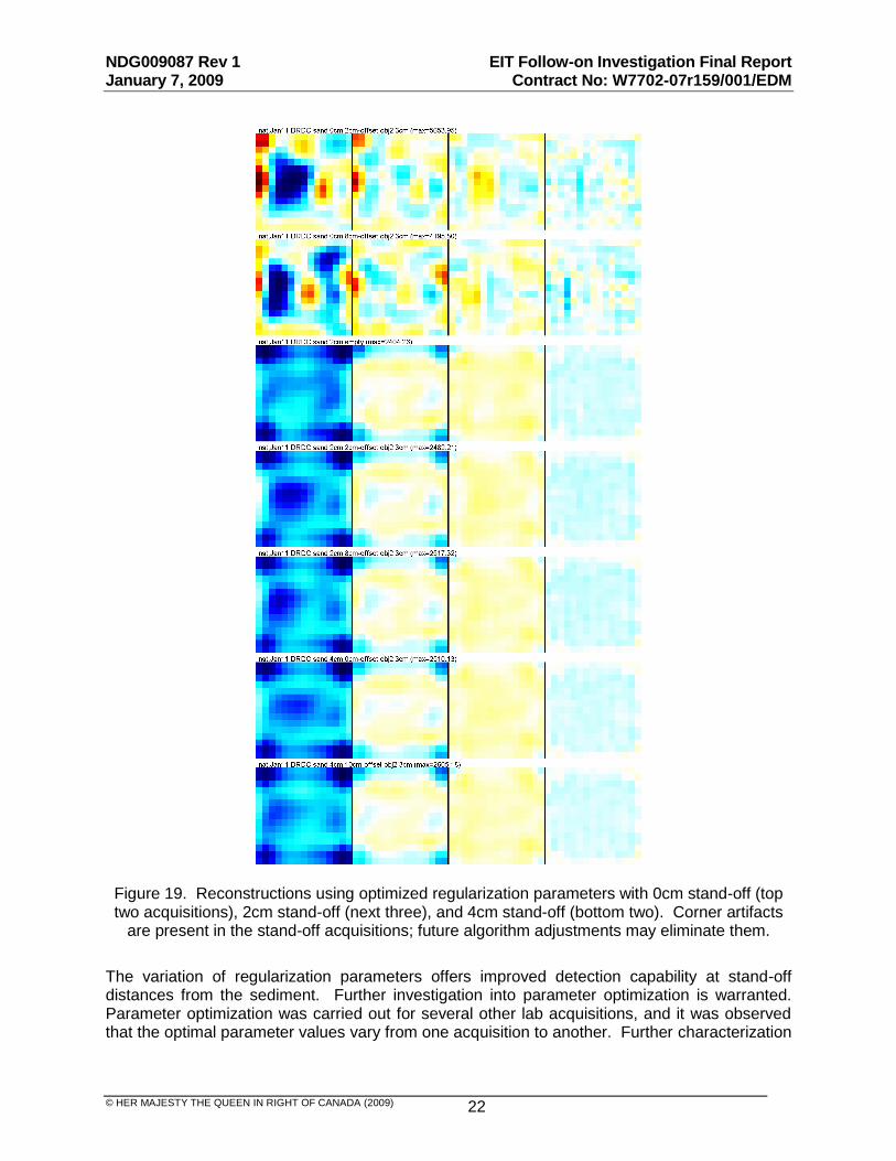
Figure 19. Reconstructions using optimized regularization parameters with 0cm stand-off (top two acquisitions), 2cm stand-off (next three), and 4cm stand-off (bottom two). Corner artifacts are present in the stand-off acquisitions; future algorithm adjustments may eliminate them. .................................................................................................................. 22
Figure 20. Reconstructions with a data weighting factor of 0.0. (The target is 13cm in diameter and 7cm tall.) ..................................................................................................................... 23
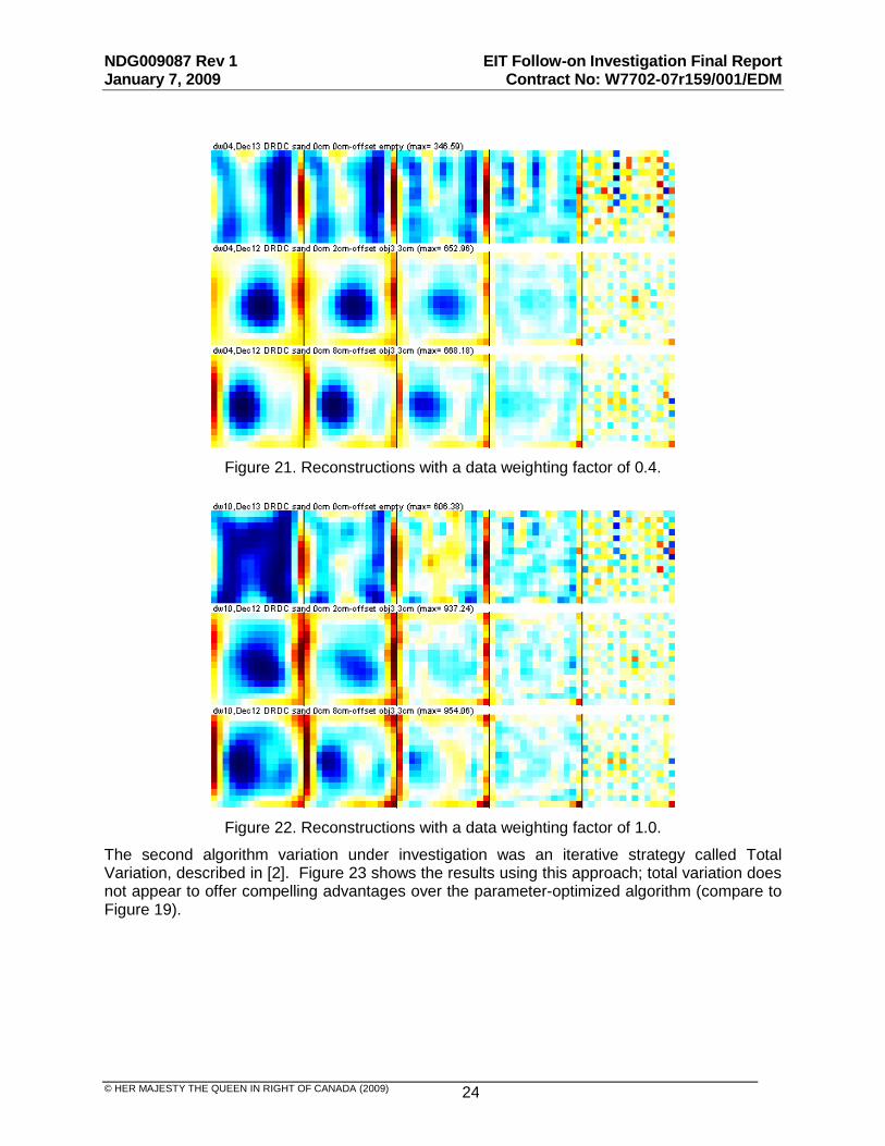
Figure 21. Reconstructions with a data weighting factor of 0.4. ................................................. 24 Figure 22. Reconstructions with a data weighting factor of 1.0. ................................................. 24 Figure 23. Reconstruction results using the total variation solver. These results are attained
after three iterations. Beyond ten iterations results diverge. .............................................. 25 Figure 24. Reconstruction results using the GREIT algorithm. .................................................. 26 Figure 25. Coarse-resolution electrode grid. ............................................................................. 28 Figure 26. Fine-resolution electrode grid. .................................................................................. 28 Figure 27. Round non-conductive test target. ............................................................................ 28 Figure 28. 40mm ammunition round. ......................................................................................... 28 Figure 29. 20mm ammunition round. ......................................................................................... 28 Figure 30. Reconstruction of the empty tank, using the coarse array. ...................................... 29 Figure 31. Reconstruction of the empty tank, using the fine array. ........................................... 29 Figure 32. Reconstruction of the non-conductive target using the coarse array. The target is
buried 2cm deep in the sediment and its dimensions are 13cm (diameter) by 7cm (height). (Due to imprecise target placement, the true location may be above the centre line, as suggested by the reconstructions.) .................................................................................... 29
Figure 33. Reconstruction of the non-conductive target using the fine array. True target location is 4cm to the right of centre. Due to imprecise target placement, the true location may be above the centre line, as suggested by the reconstructions. .............................................. 29
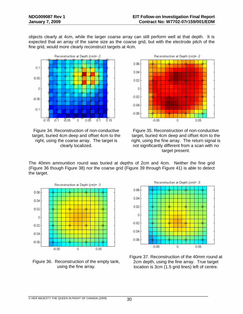
Figure 34. Reconstruction of non-conductive target, buried 4cm deep and offset 4cm to the right, using the coarse array. The target is clearly localized. ............................................. 30
Figure 35. Reconstruction of non-conductive target, buried 4cm deep and offset 4cm to the right, using the fine array. The return signal is not significantly different from a scan with no target present. .................................................................................................................... 30
Figure 36. Reconstruction of the empty tank, using the fine array. ........................................... 30 Figure 37. Reconstruction of the 40mm round at 2cm depth, using the fine array. True target
location is 3cm (1.5 grid lines) left of centre. ...................................................................... 30 Figure 38. Reconstruction of the 40mm round at 4cm depth, using the fine array. .................... 31 Figure 39. Reconstruction of the empty tank, using the coarse array. ....................................... 31 Figure 40. Reconstruction of the 40mm round at 2cm depth, using the coarse array. True target
location is vertically centred and 4cm (two grid lines) left of centre. ................................... 31 Figure 41. Reconstruction of the 40mm round at 4cm depth, using the coarse array. ............... 31

NDG009087 Rev 1 EIT Follow-on Investigation Final Report January 7, 2009 Contract No: W7702-07r159/001/EDM
© HER MAJESTY THE QUEEN IN RIGHT OF CANADA (2009) vi
Figure 42. Reconstruction of the 40mm round (wrapped in foil) at 2cm depth and 4cm offset to the right, using the coarse array. True target location is 4cm (two grid lines) right of centre.32
Figure 43. Reconstruction of the 40mm round (wrapped in foil) at 2cm depth and 4cm offset to the right, using the fine array. True target location is 4cm (four grid lines) right of centre. . 32
Figure 44 . Reconstruction of the empty tank, using the coarse array. ...................................... 32 Figure 45. Reconstruction of the 20mm round (wrapped in foil) at 2cm depth, using the coarse
array. The target is located 4cm (two grid lines) to the right of centre................................ 32 Figure 46. Reconstruction of the empty tank, using the fine array. ........................................... 33 Figure 47. Reconstruction of the 20mm round (wrapped in foil) at 2cm depth, using the fine
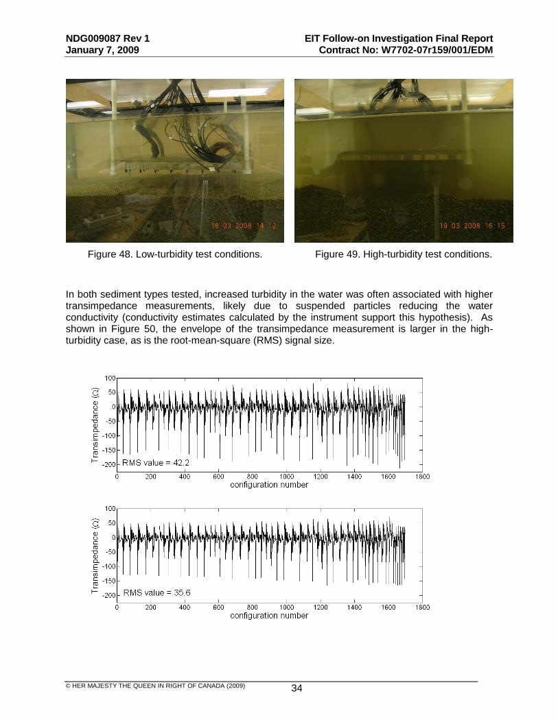
array. The target is located at the far right edge of the electrode grid. ............................... 33 Figure 48. Low-turbidity test conditions. .................................................................................... 34 Figure 49. High-turbidity test conditions. ................................................................................... 34 Figure 50. Sample transimpedance measurements for high turbidity (top) and low turbidity
(bottom) conditions. (These measurements correspond to the non-conductive object in the gravel medium.) ................................................................................................................. 35
Figure 51. Reconstruction image of a non-conducting target in low-turbidity conditions with a sand layer. The target is 13cm in diameter and 7cm tall and buried with its top surface flush with the sand surface, 4cm left of centre. The array is 4cm above the sand layer. .... 35
Figure 52. Reconstruction image of a non-conducting target in high-turbidity conditions with a sand layer. ......................................................................................................................... 35
Figure 53. Reconstruction image of a metallic target in low-turbidity conditions with a sand layer. The target is flush with the sand surface and offset 4cm to the left. It is 9cm in diameter and 4cm tall. ...................................................................................................................... 36
Figure 54. Reconstruction image of the metallic target in high-turbidity conditions with a sand layer. .................................................................................................................................. 36
Figure 55. Reconstruction of the metallic target in low-turbidity conditions with a gravel layer. .. 36 Figure 56. Reconstruction image of the metallic target in high-turbidity conditions with a gravel
layer. .................................................................................................................................. 36 Figure 57. Fine-grained sand in the test tank. ........................................................................... 37 Figure 58. Aquarium gravel of varying grain size. ...................................................................... 37 Figure 59. Reconstruction of a conductive target in sand from 2cm stand-off distance, in low
turbidity. The target is flush with the sediment surface and offset 4cm to the left. ............. 37 Figure 60. Reconstruction of a conductive target in gravel from 2cm stand-off distance, in low
turbidity. ............................................................................................................................. 37 Figure 61. Reconstruction of a non-conductive target in sand from 4cm stand-off distance, in low
turbidity. The target is flush with the sediment surface and offset 4cm to the right ............ 38 Figure 62. Reconstruction of a non-conductive target in gravel from 4cm stand-off distance, in
low turbidity. ....................................................................................................................... 38 Figure 63. Cast-iron pot used for tests, before rusting. .............................................................. 39 Figure 64. Rust test set-up. ...................................................................................................... 39 Figure 65. The cast-iron pot at the end of rust testing (rust level 11). ........................................ 39 Figure 66. Normalized measures of the magnitudes of the transimpedance measurements. ... 40 Figure 67. A reconstruction image of rust level 0. The true target position is 2cm below the
approximate centre of the array. ........................................................................................ 40 Figure 68. A reconstruction image of rust level 1. The true target position is 2cm below the
approximate centre of the array. ........................................................................................ 40 Figure 69. A reconstruction image of rust level 11. The true target position is 2cm below the
approximate centre of the array. ........................................................................................ 41 Figure 70. Lab set-up for salinity testing. ................................................................................... 42 Figure 71. Reconstruction of empty tank (1.5 g/L salinity). ........................................................ 42

NDG009087 Rev 1 EIT Follow-on Investigation Final Report January 7, 2009 Contract No: W7702-07r159/001/EDM
© HER MAJESTY THE QUEEN IN RIGHT OF CANADA (2009) vii
Figure 72. Reconstruction of target at 3 cm stand-off (1.5 g/L salinity). The target is visible, although the signal is not strong......................................................................................... 42
Figure 73. Reconstruction of target at 5 cm stand-off (1.5 g/L salinity). The target is not clearly visible................................................................................................................................. 43
Figure 74. Reconstruction of target at 7 cm stand-off (1.5 g/L salinity). The target is not discernible. ........................................................................................................................ 43
Figure 75. Reconstruction of empty tank (10 g/L salinity). ......................................................... 43 Figure 76. Reconstruction of target at 3 cm stand-off (10 g/L salinity). The target is pixelated but
visible................................................................................................................................. 43 Figure 77. Reconstruction of target at 5 cm stand-off (10 g/L salinity). The target is not clearly
visible................................................................................................................................. 44 Figure 78. Reconstruction of target at 7 cm stand-off (10 g/L salinity). The target is not clearly
visible................................................................................................................................. 44 Figure 79. Reconstruction of target at 3 cm stand-off (20 g/L salinity). The target is clearly
visible................................................................................................................................. 44 Figure 80. Reconstruction of target at 5 cm stand-off (20 g/L salinity). The target is not clearly
visible................................................................................................................................. 44 Figure 81. Reconstruction of target at 3 cm stand-off (30 g/L salinity). The target is clearly
visible................................................................................................................................. 45 Figure 82. Reconstruction of target at 5 cm stand-off (30 g/L salinity). The target is not
detectable. ......................................................................................................................... 45 Figure 83. Reconstruction of empty tank (50 g/L salinity). ......................................................... 45 Figure 84. Reconstruction of target at 3 cm stand-off (50 g/L salinity). The target is not
detected. ............................................................................................................................ 45 Figure 85. Mean Vamplitude vs. salinity (DC offset removed). The black plot corresponds to
an acquisition on the empty tank. Blue corresponds to a 3cm stand-off from the array to the non-conductive object. Red corresponds to a 5cm stand-off. ...................................... 46
Figure 86. Mean raw voltage amplitude vs. salinity (DC offset included). Plot colours correspond to the same data as in Figure 87. .................................................................... 46
Figure 88. Lab set-up for EMI detector evaluations. .................................................................. 47 Figure 89. Detection stand-off distance versus salinity for non-conductive target with metal
screw. ................................................................................................................................ 48 Figure 90. Object 2. ................................................................................................................ A-2 Figure 91. Object 3. ................................................................................................................ A-2 Figure 92. Object 7. ................................................................................................................ A-3 Figure 93. Object 8. ................................................................................................................ A-4 Figure 94. Object 11................................................................................................................ A-4 Figure 95. Object 12................................................................................................................ A-5 Figure 96. Object 14................................................................................................................ A-5 Figure 97. Object 15................................................................................................................ A-6
LIST OF TABLES
Table 1. Estimated stand-off distances and sand conductivities for various lab acquisitions, with
corresponding fit errors. ..................................................................................................... 10 Table 2. Description of test targets. ......................................................................................... A-1

NDG009087 Rev 1 EIT Follow-on Investigation Final Report January 7, 2009 Contract No: W7702-07r159/001/EDM
© HER MAJESTY THE QUEEN IN RIGHT OF CANADA (2009) 1
Executive Summary
This final report summarizes the findings obtained during the Underwater EIT Follow-on project carried out between January and October 2008 (Contract No. W7702-07r159/001/EDM). The project was intended to characterize the EIT sensing modality in various underwater conditions in view of future development of a sensing platform capable of operating in shallow water areas likely to hold mines or unexploded ordnance buried in underwater sediment. This type of environment is challenging for most landmine detection sensors. Neptec Design Group was the prime contractor for this project; Analytica was a subcontractor to Neptec.
It has been observed that the EIT technology is especially effective in wet environments. In collaboration with DRDC Suffield in 2003-04 and in 2005-06, Neptec undertook small-scale laboratory testing of an EIT instrument in an underwater environment. The results showed that the system can reliably detect targets in water if the instrument is sufficiently close to the target. This follow-on research project was designed to further evaluate the suitability of EIT for the underwater application. The main project objectives included:
Experimentation with variations on the EIT reconstruction algorithms, using the EIDORS framework.
Simulation and lab experimentation to evaluate the effects of electrode pitch on system performance.
Evaluation of EIT performance in various likely conditions for an underwater application, namely different levels of water turbidity, water salinity, and target rusting.
Comparison of EIT performance to underwater performance of a traditional EMI metal detector, under varying salinity levels.
The research into reconstruction algorithms pursued a number of potential improvements, some of which showed improvement over the original results and some of which did not. Some of the algorithms are worthy of further study.
Simulation of a fine-pitched electrode array indicated that the fine array would perform at least as well as the coarse grid for targets at a small stand-off distance. However for targets buried deeper the coarse grid performed better in simulation. Experimental results showed that shape is not more clearly discernible using the fine grid, but small targets that are too small for detection with the coarse grid may be detectable with the fine grid provided the grid is at a sufficiently small stand-off distance.
The laboratory experiments indicate that water turbidity and target rusting have little effect on EIT performance. Salinity at low levels does not affect EIT reconstruction quality, but at seawater levels detection is compromised. This failing is likely due to the material properties of the electrodes, and may be surmountable by hardware changes.
The traditional EMI detector used for comparison also deteriorates with increasing salinity, but performs better than the EIT instrument at the salinity levels of seawater.

NDG009087 Rev 1 EIT Follow-on Investigation Final Report January 7, 2009 Contract No: W7702-07r159/001/EDM
© HER MAJESTY THE QUEEN IN RIGHT OF CANADA (2009) 2
Introduction
Project Objectives:
The technical objectives of this project include the characterization of underwater mine-like object detection with regard to some key environmental parameters, such as the salinity and turbidity of the water and the rusting process. It also includes the evaluation of a finer electrode array in view of improving the spatial resolution. Another objective consists of assessing a reconstruction algorithm which is well established in the EIT research community. One last objective is to compare the underwater detection performance between an EIT and EMI detector.
This final report describes the development of the project and presents the results obtained. It is structured as follows: Section 1 lists applicable documents and references. In Section 2 the EIT system is described, including the system architecture and physical construction of the instrument. Results are presented in Section 3, including the investigation of another reconstruction algorithm, fine grid, turbidity, rust, and salinity testing, and comparison to an EMI detector. Section 4 summarizes the conclusions and recommendations resulting from the research.

NDG009087 Rev 1 EIT Follow-on Investigation Final Report January 7, 2009 Contract No: W7702-07r159/001/EDM
© HER MAJESTY THE QUEEN IN RIGHT OF CANADA (2009) 3
1 Applicable Documents & References
[1] Church, P., McFee, J., Gagnon, S., Wort, P. „Electrical ImpedanceTomographic Imaging of Buried Landmines.‟ IEEE trans. on geoscience and remote sensing, 2005.
[2] Tao Dai and Andy Adler, “Electrical Impedance Tomography Reconstruction Using L1 Norms for Data and Image Terms”, Conf. IEEE EMBS 2008.
[3] Adler, A., Arnold, J., Bayford, R., Borsic, A., Brown, B., Dixon, P., Faes, T., Frerichs, I., Gagnon, H., Gärber, Y., Grychtol, B., Hahn, G., Lionheart, W., Malik, A., Stocks, J., Tizzard, A., Weiler, N., Wolf, G. „GREIT: towards a consensus EIT algorithm for lung images.‟ 9th Conf. Electrical Impedance Tomography, Dartmouth College, Hannover, NH, USA. 16-18 June, 2008.
[4] NDG008337 Rev 1. Underwater EIT Project Final Report. Contract No. W7702-04R040/001/EDM.
[5] „Electrical conductivity and TDS‟, http://www.lenntech.com/water-conductivity.htm
NDG009087 Rev 1 EIT Follow-on Investigation Final Report January 7, 2009 Contract No: W7702-07r159/001/EDM
© HER MAJESTY THE QUEEN IN RIGHT OF CANADA (2009) 4
2 EIT System
2.1 Architecture
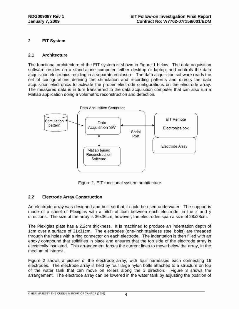
The functional architecture of the EIT system is shown in Figure 1 below. The data acquisition software resides on a stand-alone computer, either desktop or laptop, and controls the data acquisition electronics residing in a separate enclosure. The data acquisition software reads the set of configurations defining the stimulation and recording patterns and directs the data acquisition electronics to activate the proper electrode configurations on the electrode array. The measured data is in turn transferred to the data acquisition computer that can also run a Matlab application doing a volumetric reconstruction and detection.
Figure 1. EIT functional system architecture
2.2 Electrode Array Construction
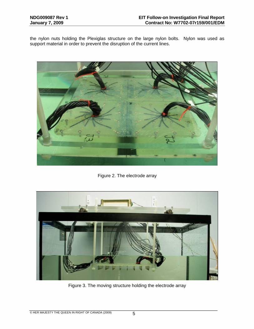
An electrode array was designed and built so that it could be used underwater. The support is made of a sheet of Plexiglas with a pitch of 4cm between each electrode, in the x and y directions. The size of the array is 36x36cm; however, the electrodes span a size of 28x28cm.
The Plexiglas plate has a 2.2cm thickness. It is machined to produce an indentation depth of 1cm over a surface of 31x31cm. The electrodes (one-inch stainless steel bolts) are threaded through the holes with a ring connector on each electrode. The indentation is then filled with an epoxy compound that solidifies in place and ensures that the top side of the electrode array is electrically insulated. This arrangement forces the current lines to move below the array, in the medium of interest,
Figure 2 shows a picture of the electrode array, with four harnesses each connecting 16 electrodes. The electrode array is held by four large nylon bolts attached to a structure on top of the water tank that can move on rollers along the x direction. Figure 3 shows the arrangement. The electrode array can be lowered in the water tank by adjusting the position of
NDG009087 Rev 1 EIT Follow-on Investigation Final Report January 7, 2009 Contract No: W7702-07r159/001/EDM
© HER MAJESTY THE QUEEN IN RIGHT OF CANADA (2009) 5
the nylon nuts holding the Plexiglas structure on the large nylon bolts. Nylon was used as support material in order to prevent the disruption of the current lines.
Figure 2. The electrode array
Figure 3. The moving structure holding the electrode array
NDG009087 Rev 1 EIT Follow-on Investigation Final Report January 7, 2009 Contract No: W7702-07r159/001/EDM
© HER MAJESTY THE QUEEN IN RIGHT OF CANADA (2009) 6
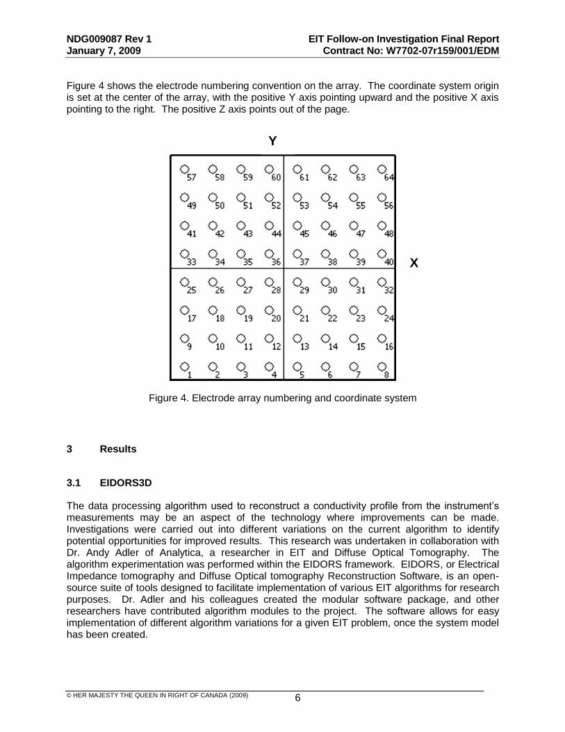
Figure 4 shows the electrode numbering convention on the array. The coordinate system origin is set at the center of the array, with the positive Y axis pointing upward and the positive X axis pointing to the right. The positive Z axis points out of the page.
Figure 4. Electrode array numbering and coordinate system
3 Results
3.1 EIDORS3D
The data processing algorithm used to reconstruct a conductivity profile from the instrument‟s measurements may be an aspect of the technology where improvements can be made. Investigations were carried out into different variations on the current algorithm to identify potential opportunities for improved results. This research was undertaken in collaboration with Dr. Andy Adler of Analytica, a researcher in EIT and Diffuse Optical Tomography. The algorithm experimentation was performed within the EIDORS framework. EIDORS, or Electrical Impedance tomography and Diffuse Optical tomography Reconstruction Software, is an open-source suite of tools designed to facilitate implementation of various EIT algorithms for research purposes. Dr. Adler and his colleagues created the modular software package, and other researchers have contributed algorithm modules to the project. The software allows for easy implementation of different algorithm variations for a given EIT problem, once the system model has been created.
X
Y

NDG009087 Rev 1 EIT Follow-on Investigation Final Report January 7, 2009 Contract No: W7702-07r159/001/EDM
© HER MAJESTY THE QUEEN IN RIGHT OF CANADA (2009) 7
The reconstruction medium under investigation must be modelled in software as part of the reconstruction process. The model describes the medium geometry as well as the location and geometry of the electrodes. The stimulation pattern, that is the sequence of stimulating and recording electrodes, is also specified in the model. The EIDORS framework runs primarily on Finite Element Models (FEM) of the medium, although other models are supported. Finite element modelling involves dividing the region of interest into many small elements over which the behaviour of the system is assumed to be uniform.
Once the model is specified, a forward and an inverse solver are required. The forward solver calculates the transimpedance measurements from the model for a given conductivity profile (which may be specified in simulation). The inverse solver uses given transimpedance measurements to determine the conductivity profile. The forward and inverse solver functions are independent of the medium model, and can be developed separately; several solvers have been provided in EIDORS by various contributors. A generic pair of solvers was used in this investigation.
The work accomplished as part of the EIDORS investigation comprises:
The recoding of Neptec‟s original algorithm and system model into the EIDORS framework.
The creation and testing of finite element models (FEMs) to model the reconstruction medium.
The explicit modelling of a dual-layer medium by specifying a sand layer in the FEM.
The investigation of advanced reconstruction algorithms allowing variation of some parameters that are implicitly hard-coded in Neptec‟s original software.
Experimentation with additional algorithm variants.
Each of these items is described below, and results are presented.
3.1.1 Recoding original algorithm for EIDORS
Neptec‟s software was re-coded to run within the modular EIDORS framework. This task was a prerequisite to carrying out the algorithm investigations using EIDORS tools. The core functions were modularized and testing and validation was performed to ensure accurate reproduction of the original algorithm.
3.1.2 Finite Element Models
The first step in the EIDORS investigation was the modelling of the medium as an FEM. For preliminary development and validation, a 2D model was generated and tested in simulation. This model described a vertical slice of the EIT reconstruction volume, including one row of electrodes and parallel to the x-z plane. Mesh refinement was carried out to increase the resolution of the model in the vicinity of the electrodes, so as to increase the accuracy of transimpedance modelling.

NDG009087 Rev 1 EIT Follow-on Investigation Final Report January 7, 2009 Contract No: W7702-07r159/001/EDM
© HER MAJESTY THE QUEEN IN RIGHT OF CANADA (2009) 8
A dual-model approach was used to give good accuracy without compromising processing time. Dual-model solutions contain two separate FEMs, one for use with the forward solver and one for the inverse solver. The forward solver is run on a more accurate model with high resolution near the electrodes, to enhance the accuracy of the model-calculated voltages. A smaller model with coarser resolution and fewer elements near the electrodes is used for the inverse solver, to reduce processing time without greatly affecting reconstruction accuracy. Figure 5 shows the 2D forward and inverse FEMs developed.
Figure 5. Dual-model 2D FEM showing forward model (in black) and reconstruction model (in blue). Electrodes are
shown in green.
Once the 2D model was developed and tested, work on a 3D model began. Several software tools were tried in the attempt to mesh the region into a 3D FEM, with the third tool yielding a useful model. Simulations were performed to test the validity of the model and various adjustments were made to improve accuracy. The round shape of the electrodes was accurately modelled, as were the insulating sleeves that cover the shaft of the electrodes (designed to force current to flow from the electrode tips). A fitting procedure was tested to compute the shape of model electrodes that best matched the measured lab data. These improvements to electrode modelling did not reduce the overall model error, and it is concluded that the inaccuracies of the model are not related to electrode geometry. Model errors are more likely due to variations in electronics and hardware.
NDG009087 Rev 1 EIT Follow-on Investigation Final Report January 7, 2009 Contract No: W7702-07r159/001/EDM
© HER MAJESTY THE QUEEN IN RIGHT OF CANADA (2009) 9
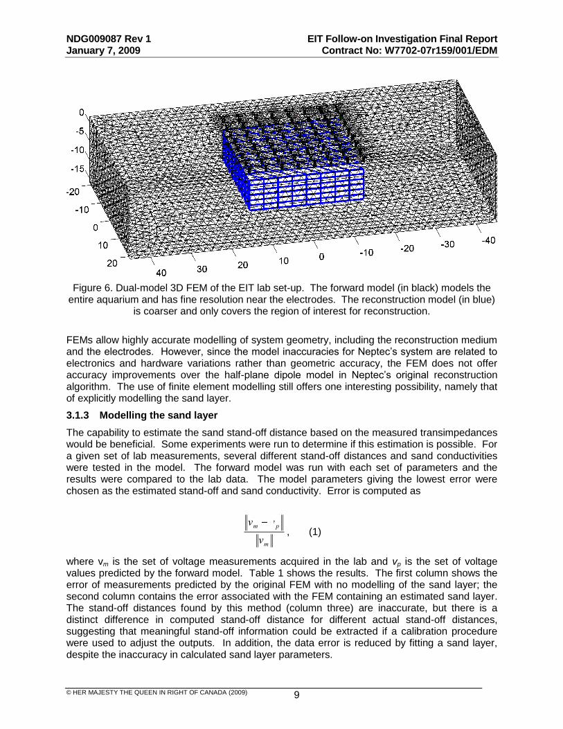
Figure 6. Dual-model 3D FEM of the EIT lab set-up. The forward model (in black) models the entire aquarium and has fine resolution near the electrodes. The reconstruction model (in blue)
is coarser and only covers the region of interest for reconstruction.
FEMs allow highly accurate modelling of system geometry, including the reconstruction medium and the electrodes. However, since the model inaccuracies for Neptec‟s system are related to electronics and hardware variations rather than geometric accuracy, the FEM does not offer accuracy improvements over the half-plane dipole model in Neptec‟s original reconstruction algorithm. The use of finite element modelling still offers one interesting possibility, namely that of explicitly modelling the sand layer.
3.1.3 Modelling the sand layer
The capability to estimate the sand stand-off distance based on the measured transimpedances would be beneficial. Some experiments were run to determine if this estimation is possible. For a given set of lab measurements, several different stand-off distances and sand conductivities were tested in the model. The forward model was run with each set of parameters and the results were compared to the lab data. The model parameters giving the lowest error were chosen as the estimated stand-off and sand conductivity. Error is computed as
m
pm
v
vv, (1)
where vm is the set of voltage measurements acquired in the lab and vp is the set of voltage values predicted by the forward model. Table 1 shows the results. The first column shows the error of measurements predicted by the original FEM with no modelling of the sand layer; the second column contains the error associated with the FEM containing an estimated sand layer. The stand-off distances found by this method (column three) are inaccurate, but there is a distinct difference in computed stand-off distance for different actual stand-off distances, suggesting that meaningful stand-off information could be extracted if a calibration procedure were used to adjust the outputs. In addition, the data error is reduced by fitting a sand layer, despite the inaccuracy in calculated sand layer parameters.

NDG009087 Rev 1 EIT Follow-on Investigation Final Report January 7, 2009 Contract No: W7702-07r159/001/EDM
© HER MAJESTY THE QUEEN IN RIGHT OF CANADA (2009) 10
The last column of Table 1 lists the file name of the lab scan. The file name describes the conditions under which the data was acquired: first the name of the sediment type appears, followed by the stand-off distance between the instrument and the sediment layer. The offset of the object (in the x direction) with respect to the centre of the array is listed next, then the object identifier and its burial depth in the sediment. A detailed description of the test objects is given in Appendix A.
Original data error
Data error with fitted sand layer
Optimized stand-off distance
Optimized sand conductivity (% of water conductivity)
Lab data used
17.2% 15.2% 4.4cm 17.9% sand_0cm_0cm-offset_empty
12.6% 9.9% 3.6cm 0% sand_0cm_0cm-offset_obj3_3cm
12.3% 10.6% 3.1cm 10.3% sand_0cm_2cm-offset_obj3_3cm
12.8% 11.1% 2.8cm 0% sand_0cm_4cm-offset_obj3_3cm
13.3% 10.8% 3.6cm 2.6% sand_0cm_6cm-offset_obj3_3cm
14.1% 12.5% 3.1cm 2.6% sand_0cm_8cm-offset_obj3_3cm
17.2% 8.9% 6.2cm 0% sand_2cm_0cm-offset_empty
20.4% 13.0% 5.9cm 0% sand_2cm_0cm-offset_ obj3_3cm
20.7% 13.6% 5.9cm 0% sand_2cm_2cm-offset_ obj3_3cm
20.6% 13.7% 5.9cm 0% sand_2cm_4cm-offset_ obj3_3cm
20.4% 13.6% 5.9cm 0% sand_2cm_6cm-offset_ obj3_3cm
20.0% 13.3% 5.6cm 0% sand_2cm_8cm-offset_ obj3_3cm
15.4% 7.3% 6.4cm 0% sand_4cm_0cm-offset_ obj3_3cm
Table 1. Estimated stand-off distances and sand conductivities for various lab acquisitions, with corresponding fit errors.
It was hypothesized that knowledge of the stand-off distance between the instrument and the sand would enable more accurate reconstruction, since the dual-layer medium could be accurately modelled. To test this hypothesis some scans were processed with a model that specified the stand-off at 0cm and again with a model specifying a 4cm stand-off. Results are shown in Figure 7 and Figure 8. Each row of images shows the reconstruction of one lab acquisition. Depth in z (with respect to the array) increases from right to left in 2cm increments, starting from 0cm.

NDG009087 Rev 1 EIT Follow-on Investigation Final Report January 7, 2009 Contract No: W7702-07r159/001/EDM
© HER MAJESTY THE QUEEN IN RIGHT OF CANADA (2009) 11
The lab acquisition details are described in the text string above each row: the parameter name and value are specified (in this case „ft‟ refers to stand-off distance), followed by the date of the acquisition and the letters DRDC. The sediment type is listed next, followed by the actual stand-off distance between the instrument and the sand layer. The lateral offset of the object with respect to the array is listed next. Finally, the object identification number and burial depth is stated, if an object is present in the scan; if not, the word „empty‟ is used to indicate the lack of target. The colour scale of the figures varies from red to blue, with white representing zero deviation from the predicted homogeneous conductivity profile. Red and yellow represent higher conductivities than predicted, with the darkness of the shade indicating greater deviation. Blue represents lower conductivities than predicted, also with shade indicating deviation.
The results in Figure 7 and Figure 8 do not differ greatly from one another, suggesting that explicit modelling of the sand layer does not improve results. There are reconstruction parameters that can be tweaked to improve performance with a stand-off, as discussed in Section 3.1.4, but system model adjustments are not helpful. Due to the lack of improvement offered by FEM modelling, the half-plane dipole model used in Neptec‟s original reconstruction software was used for the remainder of the investigation.
Figure 7. Reconstruction results with a model specifying 0cm stand-off distance.

NDG009087 Rev 1 EIT Follow-on Investigation Final Report January 7, 2009 Contract No: W7702-07r159/001/EDM
© HER MAJESTY THE QUEEN IN RIGHT OF CANADA (2009) 12
Figure 8. Reconstruction results with a model specifying 4cm stand-off distance.
3.1.4 Advanced reconstruction algorithms
The EIDORS framework allows easy comparison of various algorithms, and permits variation of some parameters that are implicitly hard-coded in Neptec‟s original software. Three parameters were tested for their effects on reconstruction quality. In this section a brief description of the algorithm formulation is provided, including the introduction of the three parameters, and the results of varying these parameters are presented.
The EIT reconstruction problem can be stated as the objective of finding a conductivity image x from transimpedance data y which minimizes
Jxy , (2)
where J is the sensitivity matrix, containing the sensitivity of each voxel in the reconstruction volume to each measurement configuration. Given certain statistical knowledge of the

NDG009087 Rev 1 EIT Follow-on Investigation Final Report January 7, 2009 Contract No: W7702-07r159/001/EDM
© HER MAJESTY THE QUEEN IN RIGHT OF CANADA (2009) 13
properties of x, such as average conductivity values and smoothness, there is an explicit expression for the x that minimizes the above norm:
yJQJJx1
. (3)
Choosing appropriate values of Q gives rise to good reconstruction images. The Q used in this research is called the NOSER prior, namely
pJJdiagQ )(*2, (4)
where diag(A) is the matrix of the same dimension as A with diagonal entries equal to those of
A and off-diagonal entries equal to zero. μ is a regularization „hyperparameter‟ that represents the inverse signal-to-noise ratio
(SNR). p is known as the image prior, and represents a weighting of data errors.
This formulation of the EIT reconstruction problem is different from the one presented in [1] and used in Neptec‟s current software, in which μ and p are implicitly defined and therefore hard-coded. In the EIDORS formulation these parameters are explicitly set and can therefore be varied to study their effects.
A third parameter, the spatial correlation, can be used to reject high-frequency noise by imposing a spatial filter on the reconstruction image. Let D be a square matrix of size equal to the number of voxels in the reconstruction volume. The elements of D are given by
1
,2
ii
sd
ij
D
jieD, (5)
where
d is the Euclidean distance between the centroids of voxels i and j.
s is the user-adjustable spatial correlation parameter.
To incorporate spatial filtering in the solution, declare
222 )(**)(*pp
JJdiagDJJdiagQ . (6)
As s approaches zero, D approaches the identity matrix and Q reduces to the original solution given in (3). For larger values of s, the conductivity image is smoothed to reduce high-frequency spatial variation.
To determine the effects of these parameter values on reconstruction quality, the image prior p was varied first. Several different values were tested to determine the optimal value for reconstruction for a particular set of scans; Figure 9 through Figure 11 show the results. Each row contains the images associated with one lab acquisition. Depth in z, relative to the array,

NDG009087 Rev 1 EIT Follow-on Investigation Final Report January 7, 2009 Contract No: W7702-07r159/001/EDM
© HER MAJESTY THE QUEEN IN RIGHT OF CANADA (2009) 14
increases from right to left in 2cm increments, starting at 0cm unless otherwise stated. The target is the most clearly visible with a prior of 0.4, although the detected depth of the object is increased somewhat. At p = 0.6, the object is pushed too far down and is less clearly visible.
Figure 9. Reconstruction results for an empty tank (top), non-conductive object at 2cm offset (centre) and the same target at 8cm
offset (bottom), for p = 0.1. This is the value implicitly used in Neptec‟s original algorithm. The object is 3cm in diameter and 7cm in
height.
Figure 10. Reconstruction results for the same scans as above, for p=0.4.

NDG009087 Rev 1 EIT Follow-on Investigation Final Report January 7, 2009 Contract No: W7702-07r159/001/EDM
© HER MAJESTY THE QUEEN IN RIGHT OF CANADA (2009) 15
Figure 11. Reconstruction results for the same scans as above, for p = 0.6.
The hyperparameter μ was also tested at several values, with results shown in Figure 12 through Figure 14. The low value of 0.01 shows noise artifacts with only a faint detection signal. The best result, showing the most smoothing and the most accurate target localization, is achieved with μ = 1.0. This value offers an improvement over Neptec‟s original algorithm.
Figure 12. Reconstructions with μ = 0.01.

NDG009087 Rev 1 EIT Follow-on Investigation Final Report January 7, 2009 Contract No: W7702-07r159/001/EDM
© HER MAJESTY THE QUEEN IN RIGHT OF CANADA (2009) 16
Figure 13. Reconstructions with μ = 0.1. This is the value implicitly used in Neptec‟s original algorithm.
Figure 14. Reconstruction results with μ = 1.0.
Finally the spatial correlation parameter was varied. Figure 15 through Figure 17 show the results. With little filtering (Figure 15), some noise is visible in upper layers. With moderate filtering (Figure 16) this noise is removed. With too high a spatial correlation penalty (Figure 17) the signal is lost.

NDG009087 Rev 1 EIT Follow-on Investigation Final Report January 7, 2009 Contract No: W7702-07r159/001/EDM
© HER MAJESTY THE QUEEN IN RIGHT OF CANADA (2009) 17
Figure 15. Reconstructions with a spatial correlation value of 0.2. (White pixels indicate zero deviation from predicted transimpedance; blue represents high deviation.)
Figure 16. Reconstructions with a spatial correlation value of 0.3.

NDG009087 Rev 1 EIT Follow-on Investigation Final Report January 7, 2009 Contract No: W7702-07r159/001/EDM
© HER MAJESTY THE QUEEN IN RIGHT OF CANADA (2009) 18
Figure 17. Reconstructions with a spatial correlation value of 0.4.
Varying these regularization parameters offers improvements in signal quality. When the three optimal values are used, the resulting algorithm offers clear improvements in detection of buried
objects at a stand-off distance for most acquisitions examined.

NDG009087 Rev 1 EIT Follow-on Investigation Final Report January 7, 2009 Contract No: W7702-07r159/001/EDM
© HER MAJESTY THE QUEEN IN RIGHT OF CANADA (2009) 19
Figure 18 and Figure 19 show Neptec‟s original algorithm results compared to the results obtained with optimized parameters, for a buried non-conductive target at different stand-off distances. In these images the top reconstruction layer has been removed and the plot colours have been re-scaled over the remaining four layers – the top layer consistently produces only noise and can therefore be ignored.
The original algorithm
(

NDG009087 Rev 1 EIT Follow-on Investigation Final Report January 7, 2009 Contract No: W7702-07r159/001/EDM
© HER MAJESTY THE QUEEN IN RIGHT OF CANADA (2009) 20
Figure 18) detects the target at 0cm stand-off: in the top two rows of the figure, the target appears as a dark blue region in a light blue medium, and the location of the signal corresponds to the true location of the target. At non-zero stand-off distances, however, the target is not reconstructed. The optimized algorithm (Figure 19) reconstructs the target reliably at 0cm stand-off, albeit less clearly than does the original algorithm (top two rows). The target appears as a dark blue region in a mottled medium, and it appears at a deeper burial depth than in the original algorithm (that is, it appears in the left-most images rather than the right-most images). At non-zero stand-off values the algorithm is able to reconstruct the target signal, unlike the original algorithm. In the deeper (left-most) reconstruction cross-sections, the target appears as a dark blue region in a lighter medium (although dark corner effects are introduced – it is a matter of future study whether these corner artifacts can be eliminated). Note that this dark target signature does not appear clearly in the scan of the empty tank (row 3), and that the signature moves laterally as the true position of the target is changed (rows 4 and 5). Even at a 4cm stand-off (bottom two rows), the algorithm reconstructs a signal that moves with the true pose of the target, indicating successful detection. Note that the detected position of the target appears deeper when the optimized algorithm is used than with the original algorithm. This occurrence may be an inevitable trade-off associated with optimized parameters, or may be corrigible – this is a subject for further research.

NDG009087 Rev 1 EIT Follow-on Investigation Final Report January 7, 2009 Contract No: W7702-07r159/001/EDM
© HER MAJESTY THE QUEEN IN RIGHT OF CANADA (2009) 21
Figure 18. Reconstructions using Neptec's original solver with 0cm stand-off (top two acquisitions), 2cm stand-off (next three), and 4cm stand-off (bottom two). The object‟s
dimensions are 14cm x 14cm x 5cm.
NDG009087 Rev 1 EIT Follow-on Investigation Final Report January 7, 2009 Contract No: W7702-07r159/001/EDM
© HER MAJESTY THE QUEEN IN RIGHT OF CANADA (2009) 22
Figure 19. Reconstructions using optimized regularization parameters with 0cm stand-off (top two acquisitions), 2cm stand-off (next three), and 4cm stand-off (bottom two). Corner artifacts
are present in the stand-off acquisitions; future algorithm adjustments may eliminate them.
The variation of regularization parameters offers improved detection capability at stand-off distances from the sediment. Further investigation into parameter optimization is warranted. Parameter optimization was carried out for several other lab acquisitions, and it was observed that the optimal parameter values vary from one acquisition to another. Further characterization

NDG009087 Rev 1 EIT Follow-on Investigation Final Report January 7, 2009 Contract No: W7702-07r159/001/EDM
© HER MAJESTY THE QUEEN IN RIGHT OF CANADA (2009) 23
of the effects of target and medium properties on optimal parameter values would be useful, and may lead to a well-understood set of criteria for determining appropriate parameter values.
3.1.5 Additional algorithm variants
Several other algorithm variants were investigated. First a data weighting approach was implemented. Using the premise that large voltage measurements are less affected by noise than small ones and are therefore more reliable, a function was implemented to weight large measurements more heavily than small ones in the reconstruction algorithm. In the basic EIT minimization problem described in Expression 2, the norm
Jxy (7)
is the Euclidean norm
2][ iJxyJxy . (8)
Data is weighted by redefining the norm as the weighted norm
2][ iiwJxyWJxy , (9)
where w
ii yW ˆ . Here y is the simulated transimpedance data for a homogeneous conductivity
profile and w is the scalar data weighting factor, which can vary between 0 (no weighting) and 1 (full weighting). Figure 20 through Figure 22 show the results for three values of w. The weighted results do not appear to offer any great improvement over unweighted reconstructions.
Figure 20. Reconstructions with a data weighting factor of 0.0. (The target is 13cm in diameter and 7cm tall.)
NDG009087 Rev 1 EIT Follow-on Investigation Final Report January 7, 2009 Contract No: W7702-07r159/001/EDM
© HER MAJESTY THE QUEEN IN RIGHT OF CANADA (2009) 24
Figure 21. Reconstructions with a data weighting factor of 0.4.
Figure 22. Reconstructions with a data weighting factor of 1.0.
The second algorithm variation under investigation was an iterative strategy called Total Variation, described in [2]. Figure 23 shows the results using this approach; total variation does not appear to offer compelling advantages over the parameter-optimized algorithm (compare to Figure 19).

NDG009087 Rev 1 EIT Follow-on Investigation Final Report January 7, 2009 Contract No: W7702-07r159/001/EDM
© HER MAJESTY THE QUEEN IN RIGHT OF CANADA (2009) 25
Figure 23. Reconstruction results using the total variation solver. These results are attained after three iterations. Beyond ten iterations results diverge.
The third and final algorithm variant studied is the Graz consensus Reconstruction algorithm for EIT, or GREIT [3]. In other EIT applications this algorithm has shown excellent uniformity of detection signal shape, regardless of the location of the target (in many algorithms, including Neptec‟s, the target signature can vary depending on its location within the region of interest). Figure 24 shows the results of the GREIT algorithm with Neptec‟s mine detection set-up, using data acquired at a 0cm stand-off. The target shape still varies with target position, showing no particular improvement over Neptec‟s original algorithm.

NDG009087 Rev 1 EIT Follow-on Investigation Final Report January 7, 2009 Contract No: W7702-07r159/001/EDM
© HER MAJESTY THE QUEEN IN RIGHT OF CANADA (2009) 26
Figure 24. Reconstruction results using the GREIT algorithm.
In summary, several of the avenues pursued did not yield improvements over Neptec‟s original algorithm. The use of finite element models and the explicit modelling of a dual-layer medium did not prove advantageous, and the three algorithm variants investigated – namely data weighting, total variation, and the GREIT algorithm – failed to produce significant gains in reconstruction quality. The area that does appear to offer promise is the variation of algorithm parameters using the advanced regularization approach. Significant improvements were observed in the ability to discern buried targets from a stand-off distance.
There are several interesting paths to pursue in future work. During this investigation the effects of varying algorithm parameters were evaluated for individual data acquisitions; the optimal parameter values changed from one acquisition to another. It would be of interest to characterize the optimal parameter values as a function of the target and medium properties, and to develop a set of optimized reconstruction parameters for various scenarios.

NDG009087 Rev 1 EIT Follow-on Investigation Final Report January 7, 2009 Contract No: W7702-07r159/001/EDM
© HER MAJESTY THE QUEEN IN RIGHT OF CANADA (2009) 27
It became obvious during the testing of FEMs that the errors between any model and the real system are likely due to features of the hardware and electronics, such as variations among amplifiers in gain and common-mode rejection ratio (CMRR) and non-zero contact impedance at the electrodes. A calibration protocol may serve to quantify and compensate for these discrepancies. The first question to answer on this subject is whether system errors can be measured by acquisitions of a known medium (e.g. a resistor network). The second step is to determine whether knowledge of the system errors can be used to improve image quality. The final challenge is to develop a practicable calibration strategy for field use. Two potential approaches to the first problem are a) modelling the electronics noise by estimating the CMRR and incorporating it into the model, and b) taking extra measurements from the hardware, for example by swapping the stimulating and recording pairs and comparing the resulting voltage values. The latter approach faces the problem that stimulation induces a polarization offset on the electrodes which attenuates over time. Sufficient time must be allowed between pair-swapping to get accurate measurements. It would be of interest to pursue this idea to determine if calibration can improve performance.
3.2 Fine Grid
Simulations and experiments were done to compare the results of high- and low-resolution electrode arrays. Simulations were processed with an electrode array having an electrode spacing of 2cm, which is half the electrode spacing of the current electrode array of 4cm. Having the same 8x8 electrode configuration as the low-resolution electrode array, the high-resolution electrode array thus spanned a square of 14x14cm, which is half the dimensions of the original electrode array of 28x28cm. Results were compared between simulations of the two different configurations, low resolution and high resolution. Simulations were done with a 1cm cube, and a 14x1x1 rectangular strip. In both cases, reconstruction and detection revealed that the high resolution performed as well as or better than the lower resolution electrode array when the object was close to the array. However, when the object met or exceeded the depth of approximately half the high-resolution electrode array length, the low-resolution electrode array outperformed the high-resolution electrode array. To examine the effects of electrode density on recognition performance in the lab, tests were performed using the pre-existing lab prototype instrument and a new finer-pitched electrode grid (see Figure 25 and Figure 26). Both arrays contain 64 electrodes arranged in an 8 x 8 grid. Electrodes in the coarse grid are at a 4cm pitch, and the array is 28cm x 28cm; the fine grid has a 2cm pitch and is 14cm x 14cm. These dimensions match those used in simulation.

NDG009087 Rev 1 EIT Follow-on Investigation Final Report January 7, 2009 Contract No: W7702-07r159/001/EDM
© HER MAJESTY THE QUEEN IN RIGHT OF CANADA (2009) 28
Figure 25. Coarse-resolution electrode grid.
Figure 26. Fine-resolution electrode grid.
Data acquisitions were taken with both grids with various targets present in the sediment. A non-conductive round object, a 40mm ammunition round, and a 20mm ammunition round were used (see Figure 27 – Figure 29). The targets were buried in the sediment at different depths, and acquisitions were taken with the electrode array touching the sand (0cm stand-off distance).
Figure 27. Round non-conductive test target.
Figure 28. 40mm ammunition round.
Figure 29. 20mm ammunition round.
The round non-conductive target was buried in the sediment at depths of 2.5cm and 4cm. At the 2.5cm depth, both the coarse and fine grids obtained a faint signal showing the target (see

NDG009087 Rev 1 EIT Follow-on Investigation Final Report January 7, 2009 Contract No: W7702-07r159/001/EDM
© HER MAJESTY THE QUEEN IN RIGHT OF CANADA (2009) 29
Figure 30 through Figure 33). Plots are colour-scaled by conductivity, with red and blue indicating non-conductive and conductive regions, respectively. The target appears larger in the fine grid since the grid itself is smaller.
Figure 30. Reconstruction of the empty tank, using the coarse array.
Figure 31. Reconstruction of the empty tank, using the fine array.
Figure 32. Reconstruction of the non-conductive target using the coarse array. The target is
buried 2cm deep in the sediment and its dimensions are 13cm (diameter) by 7cm (height).
(Due to imprecise target placement, the true location may be above the centre line, as
suggested by the reconstructions.)
Figure 33. Reconstruction of the non-conductive target using the fine array. True target location is
4cm to the right of centre. Due to imprecise target placement, the true location may be above
the centre line, as suggested by the reconstructions.
Strangely, at a burial depth of 4cm the coarse grid was able to see the target more clearly (Figure 34). The fine grid does not reconstruct a signal of the target (Figure 35). In earlier experiments [4] it was found that the size of the array determines the depth to which reliable detections can be made. The smaller extent of the fine array makes it less able to detect
NDG009087 Rev 1 EIT Follow-on Investigation Final Report January 7, 2009 Contract No: W7702-07r159/001/EDM
© HER MAJESTY THE QUEEN IN RIGHT OF CANADA (2009) 30
objects clearly at 4cm, while the larger coarse array can still perform well at that depth. It is expected that an array of the same size as the coarse grid, but with the electrode pitch of the fine grid, would more clearly reconstruct targets at 4cm.
Figure 34. Reconstruction of non-conductive target, buried 4cm deep and offset 4cm to the
right, using the coarse array. The target is clearly localized.
Figure 35. Reconstruction of non-conductive target, buried 4cm deep and offset 4cm to the right, using the fine array. The return signal is not significantly different from a scan with no
target present.
The 40mm ammunition round was buried at depths of 2cm and 4cm. Neither the fine grid (Figure 36 though Figure 38) nor the coarse grid (Figure 39 through Figure 41) is able to detect the target.
Figure 36. Reconstruction of the empty tank, using the fine array.
Figure 37. Reconstruction of the 40mm round at 2cm depth, using the fine array. True target location is 3cm (1.5 grid lines) left of centre.

NDG009087 Rev 1 EIT Follow-on Investigation Final Report January 7, 2009 Contract No: W7702-07r159/001/EDM
© HER MAJESTY THE QUEEN IN RIGHT OF CANADA (2009) 31
Figure 38. Reconstruction of the 40mm round at 4cm depth, using the fine array.
Figure 39. Reconstruction of the empty tank, using the coarse array.
Figure 40. Reconstruction of the 40mm round at 2cm depth, using the coarse array. True target location is vertically centred and 4cm (two grid
lines) left of centre.
Figure 41. Reconstruction of the 40mm round at 4cm depth, using the coarse array.
Further examination of the ammunition round revealed that a thick coat of paint provides electrical insulation, preventing it from being seen as a conductive object as originally anticipated. However, at spots where the paint is worn away a current can pass through the target. This condition causes the target to be partially insulating and partially conductive, which is a likely cause for the poor performance observed with the coarse and fine grids. To change the hybrid conductor-insulator nature of the round, it was wrapped in aluminum foil to make it entirely conductive, and the tests were repeated. In this case both arrays detected a strong conducting signal at 2cm and furthermore the long, narrow shape of the target showed up clearly in reconstructions (see Figure 42 and Figure 43). Neither array detected the target at 4cm burial depth.

NDG009087 Rev 1 EIT Follow-on Investigation Final Report January 7, 2009 Contract No: W7702-07r159/001/EDM
© HER MAJESTY THE QUEEN IN RIGHT OF CANADA (2009) 32
Figure 42. Reconstruction of the 40mm round (wrapped in foil) at 2cm depth and 4cm offset to
the right, using the coarse array. True target location is 4cm (two grid lines) right of centre.
Figure 43. Reconstruction of the 40mm round (wrapped in foil) at 2cm depth and 4cm offset to
the right, using the fine array. True target location is 4cm (four grid lines) right of centre.
The 20mm round exhibited the same characteristics as the 40mm round, being partially conductive and partially insulating; neither the coarse nor the fine grid produced clear signals at a burial depth of 3cm. When the target was wrapped in foil to make it a fully conducting target, no signal was discernible in the coarse grid acquisition at a 2cm depth (Figure 44 and Figure 45). Likely the target is too small to be detected. In the case of the fine grid (Figure 47 and Figure 46) a definitive conclusion is difficult since the target was displaced to the edge of the electrode array, or possibly beyond it (precise target placement is not possible when the object is buried from view, so there is some error in the positioning of the target with respect to the array). It appears from the C-shape of the red (low conductivity) region in the reconstruction that a higher-conductivity region has been detected near the far right edge of the array. Neither the coarse nor the fine grid detected the target at a 4cm depth.
Figure 44 . Reconstruction of the empty tank,
Figure 45. Reconstruction of the 20mm round (wrapped in foil) at 2cm depth, using the coarse array. The target is located 4cm (two grid lines)

NDG009087 Rev 1 EIT Follow-on Investigation Final Report January 7, 2009 Contract No: W7702-07r159/001/EDM
© HER MAJESTY THE QUEEN IN RIGHT OF CANADA (2009) 33
using the coarse array.
to the right of centre.
Figure 46. Reconstruction of the empty tank, using the fine array.
Figure 47. Reconstruction of the 20mm round (wrapped in foil) at 2cm depth, using the fine
array. The target is located at the far right edge of the electrode grid.
Even when covered in foil to make it more discernible as a conductor, the 20mm round was too small to be reliably detected at a 2cm depth. The detection of ammunition rounds may not be reliable using the EIT system due to the hybrid conductor/insulator nature of the rounds. The fine grid offered no noticeable improvement over the coarse grid in reconstruction quality. It was expected that the fine grid would provide more precise shape information for non-uniform shaped objects such as the ammunition rounds, but in fact both arrays provided a similar level of shape detail.
3.3 Turbidity Testing
Tests were performed to determine the sensitivity of target detection to water turbidity. With a layer of sand in the tank, the water was stirred up to increase turbidity and measurements were taken with both a conductive and a non-conductive target. The water was then allowed to sit for several days until all suspended particles settled to the bottom and the water was clear, at which point the measurements were repeated. Figure 48 and Figure 49 respectively show the water at low and high turbidity levels.
NDG009087 Rev 1 EIT Follow-on Investigation Final Report January 7, 2009 Contract No: W7702-07r159/001/EDM
© HER MAJESTY THE QUEEN IN RIGHT OF CANADA (2009) 34
Figure 48. Low-turbidity test conditions.
Figure 49. High-turbidity test conditions.
In both sediment types tested, increased turbidity in the water was often associated with higher transimpedance measurements, likely due to suspended particles reducing the water conductivity (conductivity estimates calculated by the instrument support this hypothesis). As shown in Figure 50, the envelope of the transimpedance measurement is larger in the high-turbidity case, as is the root-mean-square (RMS) signal size.

NDG009087 Rev 1 EIT Follow-on Investigation Final Report January 7, 2009 Contract No: W7702-07r159/001/EDM
© HER MAJESTY THE QUEEN IN RIGHT OF CANADA (2009) 35
Figure 50. Sample transimpedance measurements for high turbidity (top) and low turbidity (bottom) conditions. (These measurements correspond to the non-conductive object in the
gravel medium.)
In both types of sediment, reconstruction of the non-conductive target did not change with turbidity (see Figure 51 and Figure 52, where no significant difference appears). As observed in the rust testing (see Section 3.4, below), a subtle difference in transimpedance measurements does not always manifest itself in the reconstruction images.
Figure 51. Reconstruction image of a non-conducting target in low-turbidity conditions with
a sand layer. The target is 13cm in diameter and 7cm tall and buried with its top surface flush with the sand surface, 4cm left of centre. The array is
4cm above the sand layer.
Figure 52. Reconstruction image of a non-conducting target in high-turbidity conditions with
a sand layer.
Figure 53 and Figure 54 show reconstructions of the sand medium containing the conductive target, with a 2cm stand-off between the instrument and the sand. The target is flush with the sand surface. The results are very similar. Figure 55 and Figure 56 show reconstructions of the same scenario, using gravel as the sediment layer instead of sand. In the low-turbidity case (Figure 55) the object is not discernible, but it can be seen with a turbid water layer (Figure 56). In this sediment medium a higher turbidity improves the detection of metallic targets. Non-metallic targets were unaffected by turbidity changes in the gravel medium.

NDG009087 Rev 1 EIT Follow-on Investigation Final Report January 7, 2009 Contract No: W7702-07r159/001/EDM
© HER MAJESTY THE QUEEN IN RIGHT OF CANADA (2009) 36
Figure 53. Reconstruction image of a metallic target in low-turbidity conditions with a sand
layer. The target is flush with the sand surface and offset 4cm to the left. It is 9cm in diameter
and 4cm tall.
Figure 54. Reconstruction image of the metallic target in high-turbidity conditions with a sand
layer.
Figure 55. Reconstruction of the metallic target in low-turbidity conditions with a gravel layer.
Figure 56. Reconstruction image of the metallic target in high-turbidity conditions with a gravel
layer.
The sediment type appears to affect the response of the instrument to turbidity. The effects of sediment type were also studied in detail. Two different types of sediment were used during testing. The original intent was to study high- and low-turbidity conditions with sand, and to study ultra-low turbidity levels using a type of sediment, such as crystalline silica, that does not release suspended particles into the water. It was not possible to obtain crystalline silica, so a gravel was used that is designed for use in aquariums, where the water must remain clear to

NDG009087 Rev 1 EIT Follow-on Investigation Final Report January 7, 2009 Contract No: W7702-07r159/001/EDM
© HER MAJESTY THE QUEEN IN RIGHT OF CANADA (2009) 37
maintain the health of the fish. This gravel is available in a wide variety of grain sizes, and a mix of several sizes was used. Figure 57 and Figure 58 show the test set-up with both sediment types. Despite rinsing the gravel before use, significant turbidity developed when water was added to the aquarium gravel and stirred up. This development prevented the testing of ultra-low-turbidity conditions, but enabled the study of the effects of sediment type on detection.
Figure 57. Fine-grained sand in the test tank.
Figure 58. Aquarium gravel of varying grain size.
Both the conductive and the non-conductive target appear more clearly in sand than in aquarium gravel. Figure 59 and Figure 60 show reconstructions of a conductive target in sand and gravel respectively, with a 2cm layer of water between the instrument and the sediment in each case. The target is visible in the sand, but not clearly in the gravel medium. In Figure 61 and Figure 62, the experiment is repeated with a non-conductive target at a 4cm stand-off distance. The conductivity peak is better localized in the sand case.
Figure 59. Reconstruction of a conductive target in sand from 2cm stand-off distance, in low
Figure 60. Reconstruction of a conductive target in gravel from 2cm stand-off distance, in low

NDG009087 Rev 1 EIT Follow-on Investigation Final Report January 7, 2009 Contract No: W7702-07r159/001/EDM
© HER MAJESTY THE QUEEN IN RIGHT OF CANADA (2009) 38
turbidity. The target is flush with the sediment surface and offset 4cm to the left.
turbidity.
Figure 61. Reconstruction of a non-conductive target in sand from 4cm stand-off distance, in
low turbidity. The target is flush with the sediment surface and offset 4cm to the right
Figure 62. Reconstruction of a non-conductive target in gravel from 4cm stand-off distance, in
low turbidity.
It is unknown why the sand provides a better medium for detection than the aquarium gravel. The gravel is slightly more conductive than the sand, with measured conductivities 2% to 15% higher. This difference may have some effect on reconstruction. Another possible factor is the non-uniformity of the medium. Larger-grained gravel has larger interstices filled in with water, and the medium consists of many small regions of water and small regions of rock. The finer sand has smaller particles and therefore smaller interstices, so the medium is more uniform. An interesting result of the turbidity testing is the observation that transimpedance measurements are increased in high turbidity (Figure 50). This information could be very useful in a multi-sensor platform, where each sensor is assigned a reliability weighting. Water conductivity measurements from the EIT instrument could offer a means of assessing turbidity, and knowledge of the water turbidity may help in determining the reliability of different optical sensors.
3.4 Rust Testing
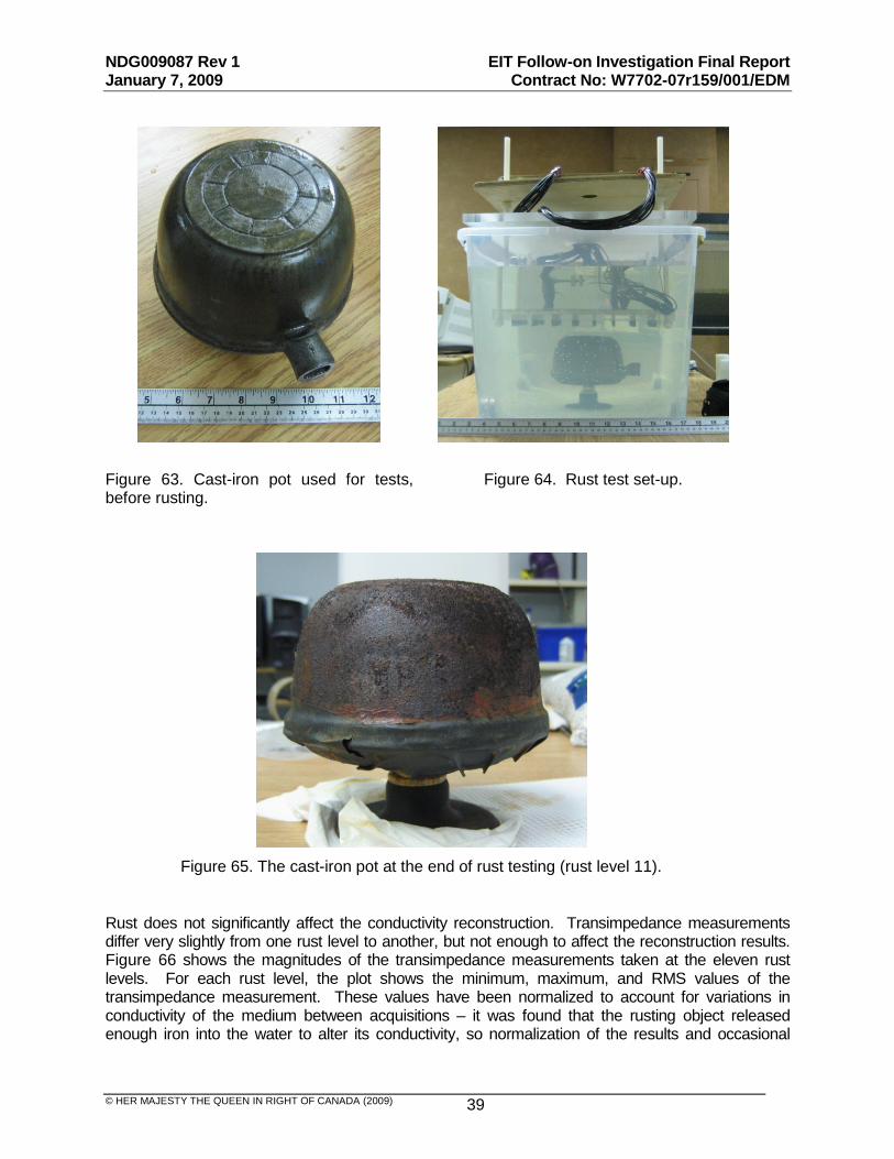
A cast-iron pot (Figure 63) was used for testing the effects of rusting on detection of metallic objects. The pot was sealed with its lid closed. Data acquisitions were taken with the object submerged in water and the sensor array positioned 2cm above it, also submerged (Figure 64). Images were taken before the object began rusting and at intervals while the object rusted. Including the un-rusted state, images were taken at eleven stages during rusting. Rusting was accelerated using vinegar to recreate the degree of rusting that would occur naturally over longer periods of time. Figure 65 shows the pot after the final acquisition.
NDG009087 Rev 1 EIT Follow-on Investigation Final Report January 7, 2009 Contract No: W7702-07r159/001/EDM
© HER MAJESTY THE QUEEN IN RIGHT OF CANADA (2009) 39
Figure 63. Cast-iron pot used for tests, before rusting.
Figure 64. Rust test set-up.
Figure 65. The cast-iron pot at the end of rust testing (rust level 11).
Rust does not significantly affect the conductivity reconstruction. Transimpedance measurements differ very slightly from one rust level to another, but not enough to affect the reconstruction results. Figure 66 shows the magnitudes of the transimpedance measurements taken at the eleven rust levels. For each rust level, the plot shows the minimum, maximum, and RMS values of the transimpedance measurement. These values have been normalized to account for variations in conductivity of the medium between acquisitions – it was found that the rusting object released enough iron into the water to alter its conductivity, so normalization of the results and occasional

NDG009087 Rev 1 EIT Follow-on Investigation Final Report January 7, 2009 Contract No: W7702-07r159/001/EDM
© HER MAJESTY THE QUEEN IN RIGHT OF CANADA (2009) 40
changing of the water were done to mitigate this effect. As the plot shows, RMS transimpedance varies very slightly from one rust level to another.
Figure 66. Normalized measures of the magnitudes of the transimpedance measurements.
Figure 67, Figure 68, and Figure 69 show reconstruction images taken from three rust levels; the same colour scale is used in all plots, so that the strengths of the signals can be compared. Figure 67 shows rust level zero (no rust on the pot); Figure 68 shows rust level one (a small amount of rust); and Figure 69 shows level eleven, the final rust level tested. The strength of the signal remains unchanged; the pot continues to appear as a conductor and give a strong detection signal. The differences between transimpedance measurements are not sufficient to produce discernible differences between reconstructions.
Figure 67. A reconstruction image of rust level 0. The true target position is 2cm below the
approximate centre of the array.
Figure 68. A reconstruction image of rust level 1. The true target position is 2cm below the
approximate centre of the array.

NDG009087 Rev 1 EIT Follow-on Investigation Final Report January 7, 2009 Contract No: W7702-07r159/001/EDM
© HER MAJESTY THE QUEEN IN RIGHT OF CANADA (2009) 41
Figure 69. A reconstruction image of rust level 11. The true target position is 2cm below the approximate centre of the array.
It is concluded, then, that the presence of rust on a metallic object does not affect the instrument‟s ability to perform detection.
3.5 Salinity Testing
The EIT instrument was tested for performance in varying levels of salt water. The tap water in the tank was used for baseline measurements at an estimated salinity of 1.5 g/L. Further tests were performed at 10 g/L, 20 g/L, 30 g/L, and 50 g/L. Note that these salinity values are low-accuracy estimates. Salinity meters were not available for testing, so the concentration of Total Dissolved Solids (TDS) was computed indirectly. The baseline salinity was calculated from conductivity measurements using interpolation between two different conversion formulas, one of which is considered reliable up to salinity levels of 1g/L; the other is reliable at higher concentrations [5]. An in-between value (between the values given by the two conversion formulas) of 1.5 g/L was chosen as the estimated baseline conductivity. This value is very approximate. Based on this value of baseline salinity and knowledge of the volume of water in the tank, the required mass of salt to reach each subsequent salinity level was calculated and added to the tank for the higher-salinity tests. No verification of these salinity levels was performed, due to the lack of salinity measurement equipment. The sediment was left in the bottom of the tank for these tests. The target was raised above the sand floor using a non-conductive support rack (Figure 70), and the array was positioned at various stand-off distances above the target. The target is of 13cm diameter and 7cm height, and was offset by 4cm in the –x direction.
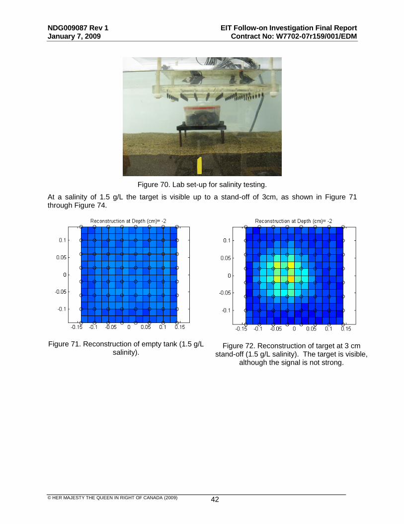
NDG009087 Rev 1 EIT Follow-on Investigation Final Report January 7, 2009 Contract No: W7702-07r159/001/EDM
© HER MAJESTY THE QUEEN IN RIGHT OF CANADA (2009) 42
Figure 70. Lab set-up for salinity testing.
At a salinity of 1.5 g/L the target is visible up to a stand-off of 3cm, as shown in Figure 71 through Figure 74.
Figure 71. Reconstruction of empty tank (1.5 g/L salinity).
Figure 72. Reconstruction of target at 3 cm stand-off (1.5 g/L salinity). The target is visible,
although the signal is not strong.
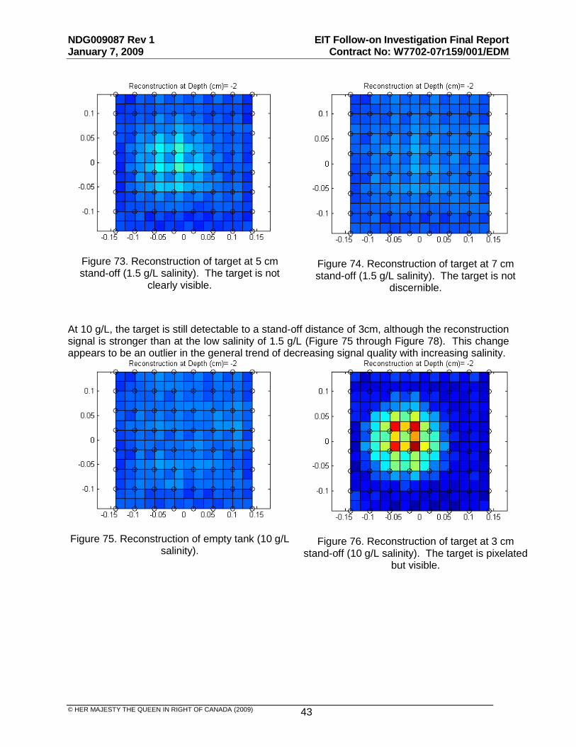
NDG009087 Rev 1 EIT Follow-on Investigation Final Report January 7, 2009 Contract No: W7702-07r159/001/EDM
© HER MAJESTY THE QUEEN IN RIGHT OF CANADA (2009) 43
Figure 73. Reconstruction of target at 5 cm stand-off (1.5 g/L salinity). The target is not
clearly visible.
Figure 74. Reconstruction of target at 7 cm stand-off (1.5 g/L salinity). The target is not
discernible.
At 10 g/L, the target is still detectable to a stand-off distance of 3cm, although the reconstruction signal is stronger than at the low salinity of 1.5 g/L (Figure 75 through Figure 78). This change appears to be an outlier in the general trend of decreasing signal quality with increasing salinity.
Figure 75. Reconstruction of empty tank (10 g/L salinity).
Figure 76. Reconstruction of target at 3 cm stand-off (10 g/L salinity). The target is pixelated
but visible.

NDG009087 Rev 1 EIT Follow-on Investigation Final Report January 7, 2009 Contract No: W7702-07r159/001/EDM
© HER MAJESTY THE QUEEN IN RIGHT OF CANADA (2009) 44
Figure 77. Reconstruction of target at 5 cm stand-off (10 g/L salinity). The target is not
clearly visible.
Figure 78. Reconstruction of target at 7 cm stand-off (10 g/L salinity). The target is not
clearly visible.
At 20g/L and 30g/L salinity, the target is still detectable at 3cm burial depth, although signal strength deteriorates (Figure 79 through Figure 82).
Figure 79. Reconstruction of target at 3 cm stand-off (20 g/L salinity). The target is clearly
visible.
Figure 80. Reconstruction of target at 5 cm stand-off (20 g/L salinity). The target is not
clearly visible.
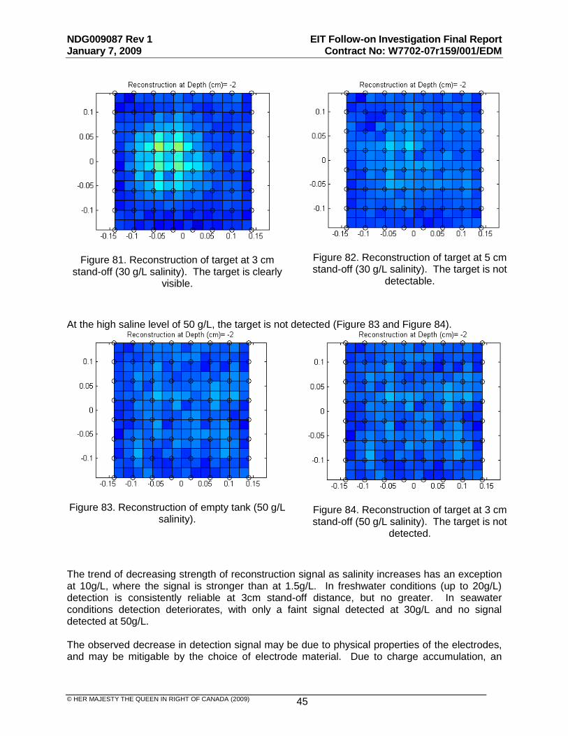
NDG009087 Rev 1 EIT Follow-on Investigation Final Report January 7, 2009 Contract No: W7702-07r159/001/EDM
© HER MAJESTY THE QUEEN IN RIGHT OF CANADA (2009) 45
Figure 81. Reconstruction of target at 3 cm stand-off (30 g/L salinity). The target is clearly
visible.
Figure 82. Reconstruction of target at 5 cm stand-off (30 g/L salinity). The target is not
detectable.
At the high saline level of 50 g/L, the target is not detected (Figure 83 and Figure 84).
Figure 83. Reconstruction of empty tank (50 g/L salinity).
Figure 84. Reconstruction of target at 3 cm stand-off (50 g/L salinity). The target is not
detected.
The trend of decreasing strength of reconstruction signal as salinity increases has an exception at 10g/L, where the signal is stronger than at 1.5g/L. In freshwater conditions (up to 20g/L) detection is consistently reliable at 3cm stand-off distance, but no greater. In seawater conditions detection deteriorates, with only a faint signal detected at 30g/L and no signal detected at 50g/L. The observed decrease in detection signal may be due to physical properties of the electrodes, and may be mitigable by the choice of electrode material. Due to charge accumulation, an
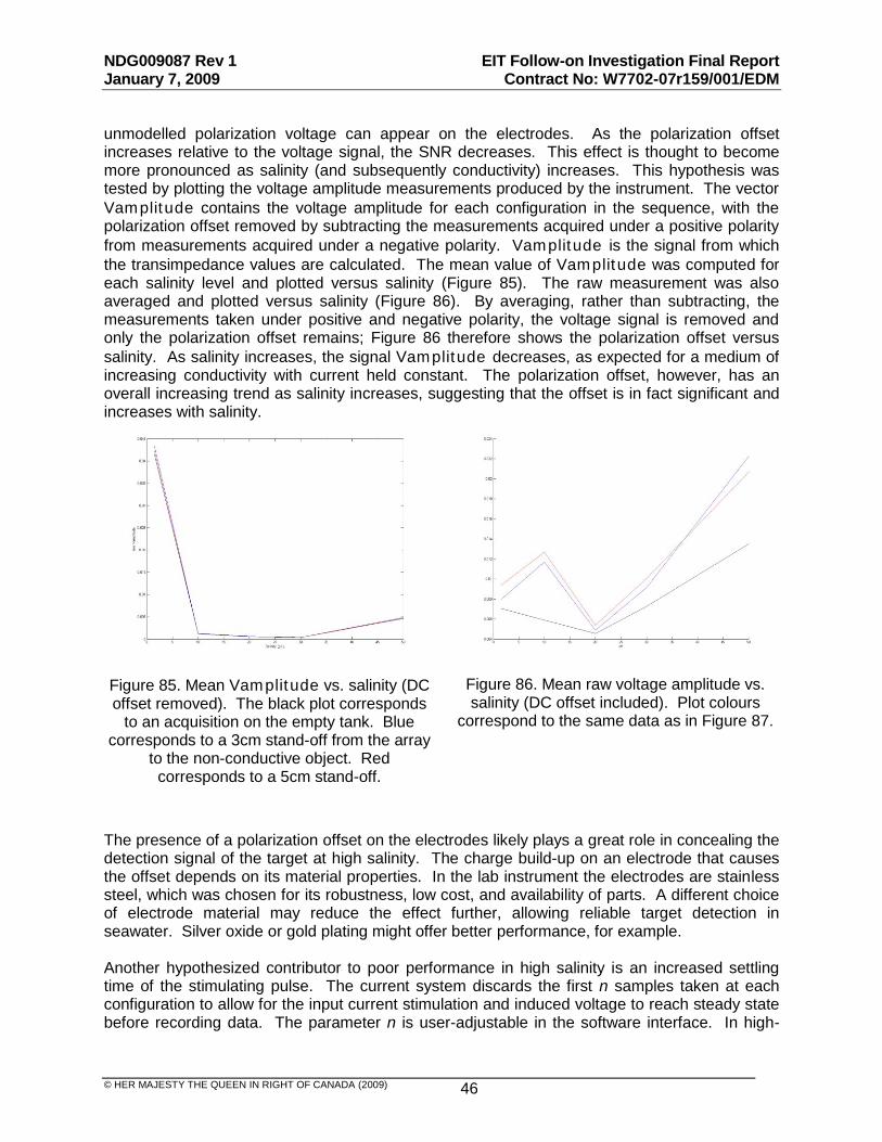
NDG009087 Rev 1 EIT Follow-on Investigation Final Report January 7, 2009 Contract No: W7702-07r159/001/EDM
© HER MAJESTY THE QUEEN IN RIGHT OF CANADA (2009) 46
unmodelled polarization voltage can appear on the electrodes. As the polarization offset increases relative to the voltage signal, the SNR decreases. This effect is thought to become more pronounced as salinity (and subsequently conductivity) increases. This hypothesis was tested by plotting the voltage amplitude measurements produced by the instrument. The vector
Vamplitude contains the voltage amplitude for each configuration in the sequence, with the polarization offset removed by subtracting the measurements acquired under a positive polarity
from measurements acquired under a negative polarity. Vamplitude is the signal from which
the transimpedance values are calculated. The mean value of Vamplitude was computed for each salinity level and plotted versus salinity (Figure 85). The raw measurement was also averaged and plotted versus salinity (Figure 86). By averaging, rather than subtracting, the measurements taken under positive and negative polarity, the voltage signal is removed and only the polarization offset remains; Figure 86 therefore shows the polarization offset versus
salinity. As salinity increases, the signal Vamplitude decreases, as expected for a medium of increasing conductivity with current held constant. The polarization offset, however, has an overall increasing trend as salinity increases, suggesting that the offset is in fact significant and increases with salinity.
Figure 85. Mean Vamplitude vs. salinity (DC offset removed). The black plot corresponds
to an acquisition on the empty tank. Blue corresponds to a 3cm stand-off from the array
to the non-conductive object. Red corresponds to a 5cm stand-off.
Figure 86. Mean raw voltage amplitude vs. salinity (DC offset included). Plot colours
correspond to the same data as in Figure 87.
The presence of a polarization offset on the electrodes likely plays a great role in concealing the detection signal of the target at high salinity. The charge build-up on an electrode that causes the offset depends on its material properties. In the lab instrument the electrodes are stainless steel, which was chosen for its robustness, low cost, and availability of parts. A different choice of electrode material may reduce the effect further, allowing reliable target detection in seawater. Silver oxide or gold plating might offer better performance, for example. Another hypothesized contributor to poor performance in high salinity is an increased settling time of the stimulating pulse. The current system discards the first n samples taken at each configuration to allow for the input current stimulation and induced voltage to reach steady state before recording data. The parameter n is user-adjustable in the software interface. In high-
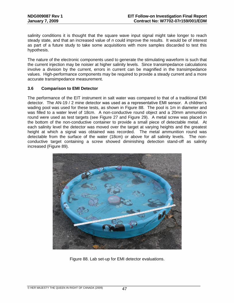
NDG009087 Rev 1 EIT Follow-on Investigation Final Report January 7, 2009 Contract No: W7702-07r159/001/EDM
© HER MAJESTY THE QUEEN IN RIGHT OF CANADA (2009) 47
salinity conditions it is thought that the square wave input signal might take longer to reach steady state, and that an increased value of n could improve the results. It would be of interest as part of a future study to take some acquisitions with more samples discarded to test this hypothesis. The nature of the electronic components used to generate the stimulating waveform is such that the current injection may be noisier at higher salinity levels. Since transimpedance calculations involve a division by the current, errors in current can be magnified in the transimpedance values. High-performance components may be required to provide a steady current and a more accurate transimpedance measurement.
3.6 Comparison to EMI Detector
The performance of the EIT instrument in salt water was compared to that of a traditional EMI detector. The AN-19 / 2 mine detector was used as a representative EMI sensor. A children‟s wading pool was used for these tests, as shown in Figure 88. The pool is 1m in diameter and was filled to a water level of 18cm. A non-conductive round object and a 20mm ammunition round were used as test targets (see Figure 27 and Figure 29). A metal screw was placed in the bottom of the non-conductive container to provide a small piece of detectable metal. At each salinity level the detector was moved over the target at varying heights and the greatest height at which a signal was obtained was recorded. The metal ammunition round was detectable from the surface of the water (18cm) or above for all salinity levels. The non-conductive target containing a screw showed diminishing detection stand-off as salinity increased (Figure 89).
Figure 88. Lab set-up for EMI detector evaluations.

NDG009087 Rev 1 EIT Follow-on Investigation Final Report January 7, 2009 Contract No: W7702-07r159/001/EDM
© HER MAJESTY THE QUEEN IN RIGHT OF CANADA (2009) 48
0
2
4
6
8
10
12
0 10 20 30 40 50 60
Salinity (g/L)
Dete
cti
on
sta
nd
-off
dis
tan
ce (
cm
)
Figure 89. Detection stand-off distance versus salinity for non-conductive target with metal screw.
The EMI detector finds the target at greater stand-off distances than the EIT detector, at all salinity levels. As discussed above, however, there are several system tweaks that may improve the performance of the EIT system in high salinity.
4 Conclusions and Recommendations
The EIDORS investigation yielded one promising area for further improvement of the reconstruction algorithm, namely the variation of advanced regularization parameters. On a scan-by-scan basis optimization of these parameters led to an improved ability to detect buried objects from a stand-off distance. It was observed that the detected depth of the target increased under these circumstances, and it is of interest to determine if this represents a corrigible weakness of the reconstruction algorithm or a fundamental trade-off associated with adjusting these parameters.
Promising further work includes the characterization of optimal parameters for different conditions, leading to an understanding of the best parameter values to use in different operational conditions. Another avenue to pursue is the possibility of developing a field-usable calibration protocol to quantify and compensate for unmodelled hardware and electronic imperfections.
The fine grid testing yielded no great improvement over the coarser grid in determining target shape. Higher electrode resolution does help detect smaller targets, however the hybrid conductor-insulator nature of ammunition rounds makes it difficult to get a reliable detection for this type of target.
NDG009087 Rev 1 EIT Follow-on Investigation Final Report January 7, 2009 Contract No: W7702-07r159/001/EDM
© HER MAJESTY THE QUEEN IN RIGHT OF CANADA (2009) 49
The turbidity of the water was found to have no discernible effect on detection of non-conductive objects. In the case of gravel sediment, increased turbidity strengthened the detection signal somewhat for metal targets. It was also found that fine sediment produces clearer results than coarse sediment.
Experimentation with a rusted target showed that detection does not deteriorate as an object rusts. No significant difference in detection signal was observed between the unrusted and the very rusted targets.
The EIT system performance degrades very slowly with increasing salinity at low salinity levels. However at a salinity of approximately 30 g/L, or low-saline seawater, the detection signal deteriorates. Comparisons to a traditional EMI detector showed that at high salinity the metal detector picks up a signal when the EIT instrument does not. It is speculated that the cause of signal degradation lies in the material properties of the lab electrodes and their tendency to accumulate charge, which decreases SNR, and in the performance of the current source circuitry. It is not necessarily the case that EIT technology is inherently unsuitable for use in high-salinity environments.
Two modifications to the EIT system may produce good reconstructions in high-salinity conditions. First, the electrode material may be affecting the results; a comparison of different electrodes would determine if improvements can be made with different materials. Second, higher-performance electronics may provide a higher-fidelity current stimulation under high-saline conditions, which would in turn improve the accuracy of transimpedance measurements. It would also be of great interest and minimal expense to take further scans with an increased number of initial discarded samples, as voltage transients may take longer to dissipate in higher salinity.


NDG009087 Rev 1 EIT Follow-on Investigation Final Report January 7, 2009 Contract No: W7702-07r159/001/EDM
© HER MAJESTY THE QUEEN IN RIGHT OF CANADA (2009)
APPENDICES

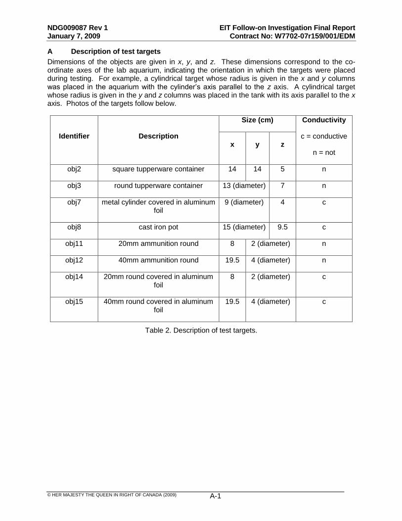
NDG009087 Rev 1 EIT Follow-on Investigation Final Report January 7, 2009 Contract No: W7702-07r159/001/EDM
© HER MAJESTY THE QUEEN IN RIGHT OF CANADA (2009) A-1
A Description of test targets
Dimensions of the objects are given in x, y, and z. These dimensions correspond to the co-ordinate axes of the lab aquarium, indicating the orientation in which the targets were placed during testing. For example, a cylindrical target whose radius is given in the x and y columns was placed in the aquarium with the cylinder‟s axis parallel to the z axis. A cylindrical target whose radius is given in the y and z columns was placed in the tank with its axis parallel to the x axis. Photos of the targets follow below.
Identifier Description
Size (cm) Conductivity
c = conductive
n = not x y z
obj2 square tupperware container 14 14 5 n
obj3 round tupperware container 13 (diameter) 7 n
obj7 metal cylinder covered in aluminum foil
9 (diameter) 4 c
obj8 cast iron pot 15 (diameter) 9.5 c
obj11 20mm ammunition round 8 2 (diameter) n
obj12 40mm ammunition round 19.5 4 (diameter) n
obj14 20mm round covered in aluminum foil
8 2 (diameter) c
obj15 40mm round covered in aluminum foil
19.5 4 (diameter) c
Table 2. Description of test targets.
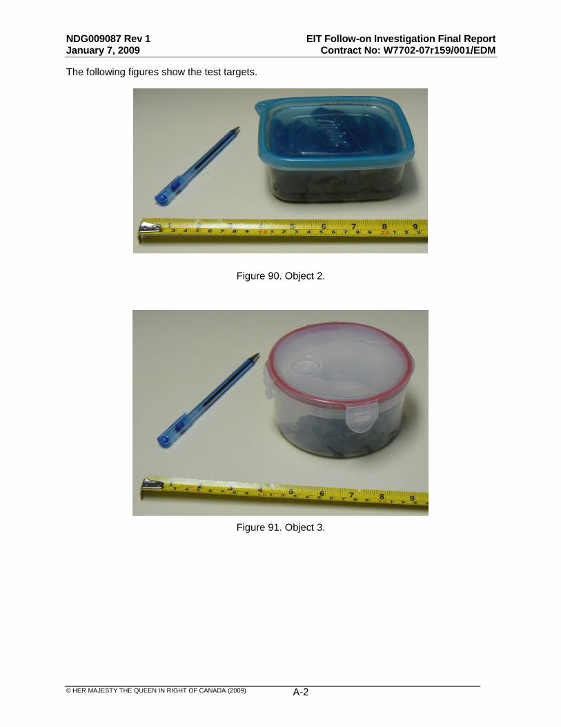
NDG009087 Rev 1 EIT Follow-on Investigation Final Report January 7, 2009 Contract No: W7702-07r159/001/EDM
© HER MAJESTY THE QUEEN IN RIGHT OF CANADA (2009) A-2
The following figures show the test targets.
Figure 90. Object 2.
Figure 91. Object 3.

NDG009087 Rev 1 EIT Follow-on Investigation Final Report January 7, 2009 Contract No: W7702-07r159/001/EDM
© HER MAJESTY THE QUEEN IN RIGHT OF CANADA (2009) A-3
Figure 92. Object 7.

NDG009087 Rev 1 EIT Follow-on Investigation Final Report January 7, 2009 Contract No: W7702-07r159/001/EDM
© HER MAJESTY THE QUEEN IN RIGHT OF CANADA (2009) A-4
Figure 93. Object 8.
Figure 94. Object 11.
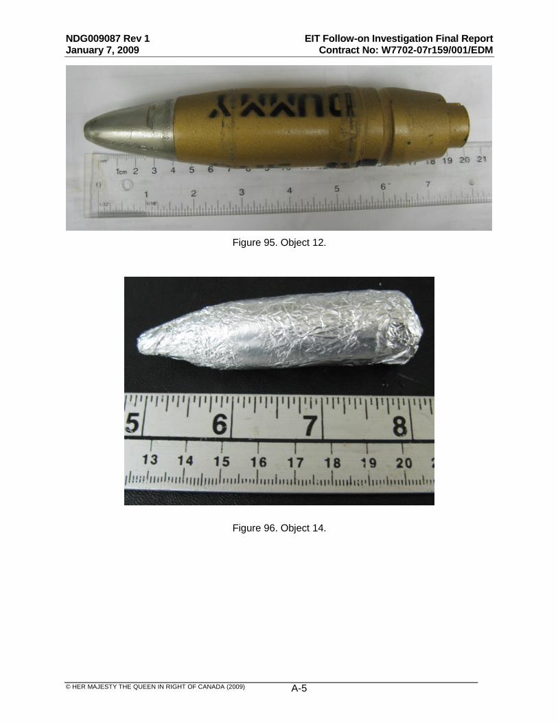
NDG009087 Rev 1 EIT Follow-on Investigation Final Report January 7, 2009 Contract No: W7702-07r159/001/EDM
© HER MAJESTY THE QUEEN IN RIGHT OF CANADA (2009) A-5
Figure 95. Object 12.
Figure 96. Object 14.

NDG009087 Rev 1 EIT Follow-on Investigation Final Report January 7, 2009 Contract No: W7702-07r159/001/EDM
© HER MAJESTY THE QUEEN IN RIGHT OF CANADA (2009) A-6
Figure 97. Object 15.

UNCLASSIFIED SECURITY CLASSIFICATION OF FORM (highest classification of Title, Abstract, Keywords)
DOCUMENT CONTROL DATA (Security classification of title, body of abstract and indexing annotation must be entered when the overall document is classified)
1. ORIGINATOR (the name and address of the organization preparing the document. Organizations for who the document was prepared, e.g. Establishment sponsoring a contractor's report, or tasking agency, are entered in Section 8.)
Neptec Design Group 302 Legget Drive Kanata ON K2K 1Y5
2. SECURITY CLASSIFICATION (overall security classification of the document, including special
warning terms if applicable)
Unclassified
3. TITLE (the complete document title as indicated on the title page. Its classification should be indicated by the appropriate abbreviation (S, C or U) in parentheses after the title).
Underwater EIT Follow-on Project Final Report
4. AUTHORS (Last name, first name, middle initial. If military, show rank, e.g. Doe, Maj. John E.)
Neptec Design Group
5. DATE OF PUBLICATION (month and year of publication of document)
January 2009
6a. NO. OF PAGES (total containing information, include Annexes, Appendices, etc) 63
6b. NO. OF REFS (total cited in document)
5
7. DESCRIPTIVE NOTES (the category of the document, e.g. technical report, technical note or memorandum. If appropriate, enter the type of report, e.g. interim, progress, summary, annual or final. Give the inclusive dates when a specific reporting period is covered.)
Contract Report
8. SPONSORING ACTIVITY (the name of the department project office or laboratory sponsoring the research and development. Include the address.)
Defence R&D Canada – Suffield, PO Box 4000, Station Main, Medicine Hat, AB T1A 8K6
9a. PROJECT OR GRANT NO. (If appropriate, the applicable research and development project or grant number under which the document was written. Please specify whether project or grant.)
Shield Thrust 12rl, 12ru
9b. CONTRACT NO. (If appropriate, the applicable number under which the document was written.)
W7702-07-R159
10a. ORIGINATOR'S DOCUMENT NUMBER (the official document number by which the document is identified by the originating activity. This number must be unique to this document.)
DRDC Suffield CR 2009-075
10b. OTHER DOCUMENT NOs. (Any other numbers which may be assigned this document either by the originator or by the sponsor.)
Neptec NDG009087
11. DOCUMENT AVAILABILITY (any limitations on further dissemination of the document, other than those imposed by security classification)
( x ) Unlimited distribution ( ) Distribution limited to defence departments and defence contractors; further distribution only as approved ( ) Distribution limited to defence departments and Canadian defence contractors; further distribution only as approved ( ) Distribution limited to government departments and agencies; further distribution only as approved ( ) Distribution limited to defence departments; further distribution only as approved ( ) Other (please specify):
12. DOCUMENT ANNOUNCEMENT (any limitation to the bibliographic announcement of this document. This will normally corresponded to the Document Availability (11). However, where further distribution (beyond the audience specified in 11) is possible, a wider announcement audience may be selected).
Unlimited UNCLASSIFIED SECURITY CLASSIFICATION OF FORM

UNCLASSIFIED SECURITY CLASSIFICATION OF FORM
13. ABSTRACT (a brief and factual summary of the document. It may also appear elsewhere in the body of the document itself. It is highly desirable that the abstract of classified documents be unclassified. Each paragraph of the abstract shall begin with an indication of the security classification of the information in the paragraph (unless the document itself is unclassified) represented as (S), (C) or (U). It is not necessary to include here abstracts in both official languages unless the text is bilingual).
This final report summarizes the findings obtained during the Underwater EIT Follow-on project carried out between January and October 2008 (Contract No. W7702-07R159/001/EDM). The project was intended to characterize the EIT sensing modality in various underwater conditions in view of future development of a sensing platform capable of operating in shallow water areas likely to hold mines or unexploded ordnance buried in underwater sediment. This type of environment is challenging for most landmine detection sensors. It has been observed that the EIT technology is especially effective in wet environments. In collaboration with DRDC Suffield in 2003-04 and in 2005-06, Neptec undertook small-scale laboratory testing of an EIT instrument in an underwater environment. The results showed that the system can reliably detect targets in water if the instrument is sufficiently close to the target. This follow-on research project was designed to further evaluate the suitability of EIT for the underwater application. The main project objectives included: experimentation with variations on the EIT reconstruction algorithms, using the EIDORS framework; simulation and lab experimentation to evaluate the effects of electrode pitch on system performance; evaluation of EIT performance in various likely conditions for an underwater application, namely different levels of water turbidity, water salinity, and target rusting; comparison of EIT performance to underwater performance of a traditional EMI metal detector, under varying salinity levels. The research into reconstruction algorithms pursued a number of potential improvements, some of which showed improvement over the original results and some of which did not. Some of the algorithms are worthy of further study. Simulation of a fine-pitched electrode array indicated that the fine array would perform at least as well as the coarse grid for targets at a small stand-off distance. However for targets buried deeper the coarse grid performed better in simulation. Experimental results showed that shape is not more clearly discernible using the fine grid, but small targets that are too small for detection with the coarse grid may be detectable with the fine grid provided the grid is at a sufficiently small stand-off distance. The laboratory experiments indicate that water turbidity and target rusting have little effect on EIT performance. Salinity at low levels does not affect EIT reconstruction quality, but at seawater levels detection is compromised. This failing is likely due to the material properties of the electrodes, and may be surmountable by hardware changes. The traditional EMI detector used for comparison also deteriorates with increasing salinity, but performs better than the EIT instrument at the salinity levels of seawater.
14. KEYWORDS, DESCRIPTORS or IDENTIFIERS (technically meaningful terms or short phrases that characterize a document and could be helpful in cataloguing the document. They should be selected so that no security classification is required. Identifies, such as equipment model designation, trade name, military project code name, geographic location may also be included. If possible keywords should be selected from a published thesaurus, e.g. Thesaurus of Engineering and Scientific Terms (TEST) and that thesaurus-identified. If it is not possible to select indexing terms which are Unclassified, the classification of each should be indicated as with the title.) Landmine detection, unexploded ordnance, underwater, electrical impedance tomography, conductivity imaging
UNCLASSIFIED SECURITY CLASSIFICATION OF FORM

Defence R&D Canada R & D pour la défense Canada Canada's Leader in Defence
and National Security Science and Technology
Chef de file au Canada en matière de science et de technologie pour la défense et la sécurité nationale
www.drdc-rddc.gc.ca