understanding the u.s. trade deficit: a disaggregated perspective

247

7.1 Introduction

By late 2005, U.S. net trade had been in deficit for more than twenty-fiveyears and was on a trajectory for more than $700 billion for the year. Indollar terms, this was the largest deficit of any country ever; as a share ofgross domestic product (GDP), it was much larger than ever experiencedby a large industrial country. Pundits, policymakers, financiers, and re-searchers wanted to know how the trade deficit got so large. They wereeven more interested in its future path.

Empirical modeling of the determinants of trade flows using the elastic-ities approach has a very long history in international economics and isused both to explain the past and to project the future. Key ingredients ofthis model are the elasticity of demand for exports and imports with re-spect to economic activity, the elasticity of exports and imports with re-spect to relative prices, and the influence of other factors, for example,global supply and increased product variety.

Given that so much work has already been done, has U.S. trade changedso as to warrant more analysis in this vein? An examination of U.S. tradepatterns over the last twenty-five years finds that the commodity and coun-try composition of trade have changed, particularly for imports. A chang-ing country and commodity composition of trade may be particularly im-portant to understand both the widening of the trade deficit and its futuretrajectory. Country composition may affect comparative advantage as newglobal supply comes on line and new trading partners appear and because

7Understanding the U.S.Trade DeficitA Disaggregated Perspective

Catherine L. Mann and Katharina Plück

Catherine L. Mann is senior fellow and Katharina Plück is research assistant at the Insti-tute for International Economics, a private, nonpartisan, not-for-profit research institute inWashington, DC.

differences in exchange rate regimes across countries may affect move-ments of relative prices. Commodity composition may matter because ofdifferent products may have differences in relative price elasticities. Inaddition, for both country and commodity composition, differences ingrowth rates of different categories of expenditure (particularly as reflectedin persistent and systematic deviation between production and absorption)in the United States compared with that of U.S. trading partners could beparticularly important in explaining the dynamics of U.S. trade and thedeficit.

This paper considers whether measures of economic activity other thanGDP better model observed trade flows. It investigates whether incomeand relative price elasticities of U.S. trade differ by trading partner or com-modity category. It asks whether new estimates of key parameters improvethe forecast performance of the trade equations. Our strategy creates adatabase of bilateral trade data for thirty-one countries, aggregates thesedetailed flows into four categories of goods based on the Bureau of Eco-nomic Analysis’s (BEA) end-use classification system—autos; industrialsupplies and materials, excluding energy (ISM-ex); consumer goods; andcapital goods. We employ trade prices and measures of expenditure thatmatch these four commodity categories and include a country-by-commodity proxy for global supply-cum-variety.

We find that using expenditure matched by commodity category is a su-perior measure of economic activity compared with using GDP and yieldsfar more plausible values for the demand elasticities. We find that the de-mand and relative price elasticities differ between industrial and develop-ing countries and across the four commodity categories. Because thecommodity composition of trade and of trading partners has changed,particularly for imports, we find that the demand elasticity for imports isnot constant. We find that industrial and developing countries have differ-ent demand and relative price elasticities for these four commodity cate-gories. We find that variety is an important variable for the behavior of cap-ital goods trade.

Comparing the in-sample performance of our specification—which dis-aggregates by product group, uses matched expenditure and trade prices,adds a variable for variety, and differentiates by trading partners’ level ofincome into industrial and developing country groups—with that of thestandard formulation of the model—which uses aggregated trade data andGDP as the expenditure variable—our disaggregated model predicts ex-ports better in-sample but does not predict imports as well as the standardformulation. Auto trade and consumer goods imports are least well ex-plained in-sample by the disaggregated model; in-sample predictions of ex-ports in each commodity category (consumer goods, autos, ISM-ex, capi-tal goods) are superior than the predictions from the standard model.

The new elasticities yield insights into the sources of the widening of the

248 Catherine L. Mann and Katharina Plück

U.S. trade deficit and have implications going forward for policymakers’approach to demand management and exchange rate regimes to rectifyglobal trade imbalances. With respect to demand management, thesenewly estimated demand elasticities across commodity categories andtrading partners imply that if U.S. consumers saved more, this would be amore important factor to change the trajectory of the trade deficit than ifour trading partners grew more. With respect to exchange rate regimes, theestimated relative price elasticities for industrial countries imply that thedollar depreciation since 2002 should affect trade with those countries, butthat significantly greater exchange rate variation on the part of developingcountries as well is needed to appreciably narrow the U.S. trade deficit.

Section 7.2 of the paper briefly reviews the vast literature on modelingU.S. international trade, focusing on the workhorse model of income andrelative prices, including its more recent variations that include proxies forglobal supply and variety. Section 7.3 presents and discusses data on theU.S. trade deficit that show changes in country and commodity composi-tion of trade, which initiated this investigation. Section 7.4 discusses ournewly constructed data. Section 7.5 presents the econometric approach.Section 7.6 discusses results and summarizes findings. Section 7.7 presentssome implications and notes areas for further work.

7.2 Literature Review

The classic workhorse model for estimating trade elasticities has beenused since at least the 1940s (Adler 1945, 1946; Chang 1945–1946). It re-lates the volume of exports or imports to real foreign and domestic incomeand relative prices (in log form):

ln trade � � � �1 ln income � �2 ln rel.price.

The model assumes that domestic and foreign tradable goods are imperfectsubstitutes, that price homogeneity holds (e.g., that an estimated coeffi-cient on the trade price and domestic price are equal, thus allowing for asingle relative price term), and that the elasticities with respect to eco-nomic activity (e.g., income) and relative prices are constant over time(see Hooper, Johnson, and Marquez [2000] for a concise summary of themodel).

All studies find—as expected—that an increase in domestic economicactivity (income) will raise the domestic demand for imports and that anincrease in foreign economic activity (income) will raise the foreign de-mand for domestic exports. A rise in the relative price of imports to the do-mestic substitute will reduce demand for imports, and a rise in the relativeprice of a country’s export good to the foreign competing good willdampen the demand for exports.

The sizes of the coefficients on income and relative price vary greatly by

Understanding the U.S. Trade Deficit: A Disaggregated Perspective 249

study, time period, countries analyzed, coverage of commodity groups,and as to whether different or additional explanatory variables are in themodel. Most studies estimate that the income elasticity for U.S. exports issmaller than the income elasticity for U.S. imports and in this regard repli-cate the earliest and most well-known finding by H. S. Houthakker andStephen Magee (1969). Subsequent studies often estimate higher exportand import elasticities than the original findings but surprisingly find thatthe ratio of the import to export elasticity varies relatively little from the 1.7found by Houthakker and Magee.1

Despite the empirical persistence of this asymmetry and its concomitantvalue for intermediate-term projections of U.S. trade flows, it is not consis-tent with global long-run equilibrium. The estimates imply that if theUnited States and the rest of the world grow at the same pace (long-runconvergence), the U.S. trade deficit would worsen, absent a trend change inrelative price2—which is also inconsistent with long-run equilibrium. Re-searchers continue to investigate U.S. trade flows and the Houthakker-Magee asymmetry by examining different data samples, considering moreprecise measures for certain variables, employing different estimation tech-niques, and adding new independent variables to the basic Houthakkerand Magee specification.

One approach to the Houthakker-Magee asymmetry is to evaluatewhether changes in the commodity composition of U.S. trade over the pasttwenty-five years changes the elasticities. For example, researchers havefound different income and price elasticities for different product cate-gories (see Stone [1979] and Marquez [2002] for different goods categories;see Sawyer and Sprinkle [1996] for a survey; see Deardorff, Humans, Stern,and Xiang [2001] and Mann [2004] for services). Hooper, Johnson, andMarquez (2000) cannot reject the hypothesis that the U.S. trade elasticitiesare constant over time, but they hold the country composition of tradefixed at the 1995 shares and, because of data availability and the objectiveof the study, focus on industrial-country trade. On the other hand, using a


1. Houthakker and Magee (1969) estimated the U.S. income elasticity for total imports of1.7 (autocorrelation corrected estimate in the appendix) and the foreign income elasticity forU.S. exports at around 1. In their survey of import and export demand elasticities for theUnited States, Sawyer and Sprinkle (1996) find income elasticities for total merchandise im-ports ranging from 0.1322 (Welsch 1987) to 4.028 (Wilson and Takacs 1979). Estimates forforeign income elasticities for U.S. exports do not vary quite as much; still they range from0.374 (Stern, Baum, and Greene 1979) to 2.151 (Wilson and Takacs 1979). The median(mean) estimate of the twenty-four studies on total U.S. imports referenced in Sawyer andSprinkle is 2.02 (2.14). The median (mean) estimate of the seventeen studies on total U.S. mer-chandise exports referenced in Sawyer and Sprinkle is 1.12 (1.02). In one of the more recentstudies, Hooper, Johnson, and Marquez (2000) find that the long-run income elasticities forU.S. exports and imports are 0.8 and 1.8, respectively, and are stable over time. See also dis-cussion in Mann (1999, 123–26).

2. Krugman and Baldwin (1987), among others, make this observation and discuss impli-cations.

century of data, Marquez (1999) finds that the elasticity with respect to in-come for U.S. imports varies over time as trade openness affects the shareof imports in expenditure.

Researchers have also focused on “the notorious inadequacies of importand export price indexes” (Houthakker and Magee 1969, 112). Relativeprice measures used most often to proxy for domestic substitutes for thetraded product—the GDP deflator and the wholesale price index—intro-duce bias because both include a considerable share of nontraded goods(Goldstein and Khan 1985). Moreover, conventional price indexes fortraded goods are too aggregated to reflect new product introductions andmay not take account of the effect of changes in global supply on prices andtherefore on demand, which apparently have been important features ofcurrent data.3 Incorporating different price indexes changes the estimatedincome elasticities in the workhorse model. In a narrow investigation,Feenstra’s (1994) detailed work on prices of six narrowly defined manufac-turing goods substantially reduced the estimated income elasticity of U.S.import demand for these six products.4 Marquez (2002) constructs a rela-tive price variable using Feenstra’s price-index methodology and also in-cludes a type of relative capital stock term originally used in Helkie andHooper (1988); his estimation reduced income elasticities for U.S. importsof producer goods, but not of services or consumer goods.

Constructing new price indexes is outside the scope of most empiricalwork, so researchers have focused on putting auxiliary variables in thestandard regression to account for changes to supply and demand that maynot be incorporated into price indexes. The sign and size of any suchsupply-cum-variety variables is not clear. If new trading countries simplyincrease global supply, global prices would tend to fall and thus increasedemand for their exports. But according to Paul Krugman’s (1989) “45-degree rule,”5 such fast-growing countries produce more varieties with in-


3. Broda and Weinstein (2004) show that between 1972 and 2002 the number of varietiesimported by the United States increased by 252 percent (15), with an important source of thenew varieties being the entry into global trade of dynamic emerging-market economies in-cluding China, Taiwan, Korea, India, and Mexico. Hummels and Klenow (2004) find that ascountries industrialize and grow, not only do their exports increase in nominal value but alsothe breadth of variety these countries offer to the world widens. Schott (2004) shows that va-rieties within a product set differ systematically across countries, with higher unit-value vari-eties coming from countries with higher productivity. See also Funke and Ruhwedel (2001).

4. Feenstra considers imports of men’s leather athletic shoes, men’s and boys’ cotton knitshirts, stainless steel bars, carbon steel sheets, color television receivers, and portable type-writers, and, for comparison purposes, gold and silver bullion between 1967 and 1987. Hetreats as variety a good from a particular country (often termed the Armington assumption)and calculates each variety’s share in actual U.S. expenditure and the U.S. elasticity of substi-tution between those different varieties. This method takes account of the new varieties pro-duced (in this case, equivalently new trading partners) and exported in ever greater quantitiesby developing countries, for example.

5. It is called the “45-degree rule” because the growth rates and the ratio of export to im-port income elasticities for countries can be plotted as a 45-degree line between two axes.

creasing returns to scale and should not experience a deterioration of theirtrade balance (and therefore face steady depreciation of their currency) be-cause consumers love varieties. Given income, the apparent demand curvefor the varieties shifts out, and there is no deterioration in the terms oftrade. Peter Schott (2004) finds that fast-growing countries with high pro-ductivity growth produce varieties that are high unit value, so for them thedemand curve is not only shifting out but also tilting in their favor.

The classic workhorse model (of equation [1]) using the standard com-plement of income and relative prices may not take account of the effectthat trading partners’ supply or variety of exports have had on U.S. importprices or import demand. The U.S. import elasticity would tend to be over-estimated to the extent that some of the explanation for the rising share ofimports in U.S. GDP lies with increased foreign supply (and thus lowerprices and thus more demand for imports); and some of the explanationcomes from increased domestic taste for variety, holding income constant.Researchers have implemented the global supply-cum-variety measure us-ing several variables.

• Helkie and Hooper (1988) use the ratio of home to foreign productivecapital stocks to represent exporters’ increased capacity to supplymore new products to the U.S. market. Their new variable significantlyreduced the inequality between income elasticities for U.S. importsand exports for the time period of their estimation. But in later workusing more recent data, the variable is no longer econometrically sig-nificant.

• Bayoumi (1999) includes exporters’ GDP in a panel estimation fortrade flows between 21 industrial countries. He finds that this supplyeffect is significant and increases in the longer run;6 the importer’s es-timated income elasticity decreases over time.

• Marquez (2002) considers immigration as a proxy for American con-sumers’ tastes for varieties from abroad. With a growing share of im-migrants in the population, he posits that U.S. demand for importsfrom immigrants’ home countries must be higher, all other thingsheld equal. Including the immigration variable does reduce the esti-mated U.S. income elasticities for services and consumer goods im-ports.

• Gagnon, in three recent papers (2003a,b, 2004), finds a significantsupply effect (defined as potential output growth or relative GDP ofthe exporting country). Including this supply variable reduces the co-efficient on income in a U.S. import regression. His results for U.S. ex-ports are less robust.


6. The fact that the coefficient on exporters’ output increases with increasing lags showsthat it is the exporting countries’ potential growth that determines its capacity to supply va-riety, not short-run fluctuations in growth rates.

• Similarly, Cline (forthcoming) puts the trading-partner GDP into theworkhorse model and finds that it reduces the income elasticities inU.S. trade equations for both exports and imports.

To summarize, considering changes in trading partners and commoditycomposition of trade, using more disaggregated trade prices, and takingbetter account of global supply or demand for variety are the predominantdirections of the research to date. We will continue in these directions andalso investigate the income variable itself, collecting data that bettermatches this variable to the disaggregated commodity and country com-position of trade. So there are five dimensions for our analysis: tradingpartner, composition of trade, variety-cum-global supply, measures of eco-nomic activity, and trade prices.

7.3 Graphical Evidence to Support a Disaggregated Approach

Figure 7.1 and table 7.1 display the commodity decomposition of U.S.merchandise trade and are key spurs to this investigation.7 Figure 7.1shows the U.S. trade deficit disaggregated into the BEA’s end-use cate-gories of capital goods, ISM-ex, consumer goods, and autos and autoparts. (For completeness, the figure also shows net trade in “other”—pe-troleum and agricultural products.) The bulk of the deterioration in thetrade deficit can be accounted for by a widening deficit in autos, consumer


7. Detailed presentation of all the data is available in the appendix figures in Mann andPlück (2005).

Fig. 7.1 U.S. trade balance by principal end-use categories, billions of U.S. dollarsSource: Bureau of Economic Analysis, International Transactions Accounts Data.

goods, and oil. Capital goods and ISM-ex appear to be more global pro-cyclical.

Table 7.1 decomposes export and imports into these same commoditygroups. The largest categories of both imports and exports are capitalgoods and ISM-ex; from 1980 to 2004, the share of capital goods rose andthat of ISM-ex fell. Capital goods is a particularly interesting category be-cause of the potential importance of changing global supply and variety.Moreover, from a macroeconomic perspective, global investment cyclesmay differ from global GDP cycles, with consequences for U.S. capitalgoods exports and imports. Consumer goods is a large category with adramatic increase in the share of U.S. merchandise imports, rising from 14to 25 percent in twenty-five years. The share of consumer goods in totalmerchandise exports rose only modestly and accounts for only 13 percentof exports. Consumer goods constitute a particularly interesting categorybecause of the potential role of changes in country source of supply.Moreover, from a macroeconomic perspective, differential growth in per-sonal consumption expenditures in the United States versus that in trad-ing partners may be an important factor in the widening of the U.S. tradedeficit.

Table 7.2 shows that the country composition of trade, particularly of im-ports, has changed dramatically.8 Trade with the industrial countries ingeneral has stayed relatively stable, with the share of imports remaining atabout 50 percent and that of exports falling from 60 to 55 percent (1980 to2004). Within the industrial-country group, exports to Europe and Japanhave fallen. The share of imports from certain developing countries and re-gions has changed dramatically, with the share of imports from China in-creasing from basically 0 to 13 percent over the period, the share of exports


Table 7.1 Trade share by principal end-use category (%)

Imports Exports

1980 2004 1980 2004

ISM-ex 31 26 29 14Capital goods 34 40 13 23Consumer goods 8 13 14 25Autos 8 11 11 15Other 20 12 43 23

Memo: Trade as a share of GDP 10.7 15 9.4 9.8

Source: Bureau of Economic Analysis, International Transactions Account data, table 2.Notes: ISM-ex � industrial supplies and materials, excluding oil. “Other” defined as petro-leum products and feeds, foods, and beverages.

8. Additional detail on these data can be found in appendix figures A2.1 and A2.2 in Mannand Plück (2005).

to Mexico doubling to 11 percent, and the share of trade with Latin Amer-ica (less Mexico) contracting.

Putting the evidence on commodities and countries together with the evo-lution of trade flows and the trade deficit suggests that closer inspection oftrade flows by country and commodity is warranted. However, the BEA doesnot publish bilateral trade data by merchandise categories. The Census Bu-reau’s published trade data by category and trade partner does not extendback further than 1995, and the United States International Trade Commis-sion (USITC) database covers bilateral trade by product only from 1989.Hence, we turn to another comprehensive source of a long time series of datato analyze the changing commodity-and-country composition of U.S. trade.

7.4 Our Database on U.S. Trade Commodity—By Country

Our empirical investigation of trade by commodity and country requiresa new database of disaggregated bilateral trade; it also requires additionalcountry and commodity-specific data. Our database includes (a) a thirty-one-country sample of bilateral trade with the United States aggregatedinto four commodity groups so as to replicate the BEA’s main end-use cat-egories; (b) expenditure data matched by country and matched to the com-modity groups; (c) trade prices matched to the commodity groups, andrelative prices matched by country and commodity group; and (d) asupply-cum-variety proxy for each commodity group.

7.4.1 Constructing Bilateral Trade Data

To approximate our initial evidence derived using BEA data and be-cause we use the Bureau of Labor Statistics’s (BLS) trade price indexes that


Table 7.2 Trade shares by country/region (%)

Exports Imports

1980 2004 1980 2004

Europe 32 23 19 22Canada 19 24 17 18Mexico 7 14 5 11Japan 9 6 13 9China 2 4 0 13Asia without China and Japan 15 18 20 17Latin America without Mexico 11 8 10 7Australia 1 2 1 1Other 5 2 15 3

Source: Bureau of Economic Analysis, International Transactions Accounts Data.Note: “Other” includes Africa and international organizations.

are matched to the BEA categories, we recreate the BEA’s end-use cate-gories using the Standard International Trade Classification (SITC, Revi-sion two-, four-, and five-digit), which in the United Nations Comtradedatabase spans the longest time period. To match BEA’s end-use commod-ity groups, we use Comtrade’s raw materials and intermediate goods forour “ISM-ex” category; “capital goods” encompasses most of SITC chap-ter 7 and some categories in chapter 8; “autos” includes passenger vehiclesand their parts from chapter 7; and “consumer goods” is made up almostentirely of the categories comprising chapter 8. We excluded all of chapter3 (energy) and all of chapter 1 (food) as these are also excluded from theBEA’s end-use categories that are the focus of our graphical evidence.Table 7A.1 in the appendix shows the complete list.

For our econometric technique, we need a uniform panel with the sameset of countries for each of the commodity groups for both imports and ex-ports. To select countries to include in the database, we start with bilateraltrade between the United States and partner countries by each four-digitor five-digit SITC category. For each country reporting trade data to theUnited Nations, we calculated its share in U.S. total merchandise importsand total merchandise exports and its share in trade in each of our fourcommodity groups. Of all countries in the database, we selected those thatrepresented the first 90 percent of trade in each category. We excluded mostof the Middle East because of the suspicion that trade with these countriesmight not be well estimated with the income and relative price formulationof the standard workhorse model. We excluded the countries of the formerSoviet Union because there are insufficient data on expenditure and prices.We also excluded South Africa. Hence, our sample of bilateral trade pairsincludes thirty-one countries from Asia and the Pacific, North America,Latin America, and Western Europe.9

Because of our intended econometric approach, some variation in coun-try composition across the commodity groups is ignored. For example,Bangladesh, Honduras, and Sri Lanka are excluded; even though they arein the first 90 percent of U.S. imports of consumer goods, they were not im-portant trading partners in the other end-use categories. At the other ex-treme, we included thirty-one countries in U.S. auto imports and exportseven though the United States trades autos and parts overwhelmingly withCanada, Mexico, Japan, and Germany.10


9. Trade data on thirty countries are from the United Nations’s (UN) Comtrade database.Data on a comparable basis for Taiwan come from that country’s statistical office.

10. Our econometric estimates in this paper confirm that the coefficients differ across thecommodity-and-country composition of trade. In a subsequent analysis, we will drop the re-quirement to have a uniform panel and allow the country composition of the commoditygroups to vary. As noted later, this may improve the in-sample predication of imports of au-tos and consumer goods.

Figure 7.2 shows one example—imports of capital goods—of how sig-nificant is the change over time in the country-by-commodity shares.11

To employ the workhorse model of trade, we need real exports and realimports. We deflate all nominal values by the corresponding end-use ex-port and import price indexes from the BLS’s International Price Pro-gram.12

7.4.2 Constructing Matched Expenditure Variables and Relative Prices

A key part of the analysis is whether the elasticities estimated in the work-horse model differ by the measure of economic activity employed. The stan-dard measure of economic activity used in trade equations is real GDP. Al-though this makes sense in aggregated trade equations, given the commodityfocus of this paper, superior elasticity estimates may be generated by bettermatching the activity variable to the type of traded commodity.

We construct country-specific measures of real consumption expendi-


Fig. 7.2 Regional or country shares of U.S. capital goods imports (percent)Source: United Nations Comtrade database.

11. See appendix figures A4.1 to A4.8 in Mann and Plück (2005) for detailed presentationof the country-by-commodity data over 1980 to 2003.

12. The end-use import and export prices do not differentiate by trading partner. Inspec-tion of some country-specific time series data from the BLS rejects the assumption that pricesdo not vary by trading partner. However, country-specific trade-price data are unavailable atsufficient time series length and are not disaggregated on an end-use basis.

ture, investment, and GDP from the Penn World Tables.13 On the importside, U.S. real GDP, real consumption expenditure, and real investment areall from the National Income and Product Accounts (NIPA) tables. In theestimation, we use real consumption expenditures in the trade equationsfor consumer goods and autos and real investment expenditures in thetrade equations for ISM-ex and capital goods.14 Notably, real investmentgrowth is much more volatile than GDP, and real consumption growth andreal GDP growth diverge for extended numbers of years in the 1980s and1990s.

There is another rationale for using a different measure of economic ac-tivity than GDP. The systematic deterioration of the U.S. current accountdeficit and the comparable rise in current account surpluses around theworld (as documented in Truman [2005] and Mann [2005]) suggest a sys-tematic bias in GDP as a measure of economic activity. For chronic surpluscountries, GDP growth as a measure of activity generating demand forU.S. exports may be too high as domestic demand growth is less than GDPgrowth by the share of net exports in those countries’ GDPs. For thechronic U.S. deficit, GDP growth as a measure of activity generating de-mand for U.S. imports may be too low as domestic demand growth isgreater than GDP growth by the share of net imports in U.S. GDP. A keyeconometric exercise is to compare the estimated demand elasticitiesacross these alternative measures of economic activity, controlling forcountry and commodity-specific effects.

In our analysis, we take the relative price variable of the workhorsemodel (trade price relative to domestic competing substitute) as givenrather than estimate a system of trade and price equations.15 We constructrelative prices for U.S. imports as the ratio of the end-use specific importprice index from the BLS and the corresponding U.S. domestic price indexfrom the BLS: The producer price index (PPI) is used for ISM-ex and cap-ital goods. The consumer price index (CPI), excluding energy and foodprices, is used for consumer goods and autos. To construct relative exportprices, we converted the dollar-based end-use–specific export price index


13. We generate real measures of expenditure by multiplying the real per capita values bypopulation. Because the Penn data only extend through 2000, we use the growth of theseexpenditure categories from the IMF’s International Financial Statistics (IFS) deflated bydomestic producer price or consumer price indexes to complete the time series to 2003. For adiscussion of purchasing power parity (PPP)–adjusted data versus market exchange rate–adjusted data when undertaking comparative country analysis, see Castles and Henderson(2005).

14. Appendix figure A3.1 in Mann and Plück (2005) shows the various export-weighted for-eign activity variables and various U.S. activity variables.

15. Most recent studies estimate prices as part of a set of simultaneous equations (Hooper,Johnson, and Marquez 2000). While researchers have always warned of the bias that may beintroduced by treating relative prices as exogenous, several recent studies could not confirmthat the coefficient on economic activity changed when including different formulations ofthis price variable or when allowing for simultaneity.

from the BLS into foreign currency using current market exchange ratesand divided by the respective trading partner’s price index (using CPI orPPI depending on the commodity group, as for the U.S. data).16 Notably,over the twenty-three-year period, the relative price of capital goods ex-ports and imports exhibit more variation than the relative price of all im-ports and exports; the relative price of consumer goods imports shows rel-atively less variation.

7.4.3 Constructing Variety

Recent literature has focused on adding variables to the workhorsemodel, in part to address the issues, as previously discussed, that have notbeen embodied in official price indexes. A global supply variable could ac-count for entry of dynamic emerging-market economies into global tradeand proxy for an outward shift of the global supply curve, which enablesthe United States to buy more imports at lower prices. A variety variablecould account for differences in quality of goods within a commodity cat-egory and how variety in imports (exports) available to U.S. consumers(foreign buyers) has grown. Such quality or variety shifts and changes intaste may not be incorporated into the price indexes we use, hence biasingthe overall regression.

Following Broda and Weinstein (2004) as well as Gagnon (2003b), weconstruct a variety proxy by counting the number of SITC four-digit cate-gories that are included in each commodity group for a given country ineach year. To compare the growth in variety across countries and cate-gories, we set the number of categories equal to 100 in the first year of ourpanel. Similar to Broda and Weinstein, we find that the growth in varietywas modest for the industrial countries; emerging-market economies onthe other hand substantially increased their supply of variety to the UnitedStates.

The growth in variety was especially great for capital goods imports—with the number of SITC categories provided by China having grown bymore than 250 percent.17 In 1980, China provided only forty-six categoriesunder the capital goods heading, with “metalworking machine tools” be-ing the biggest in nominal dollar terms ($18 million); in 2003, China sup-plied 125 goods out of a possible 136 four-digit categories in capital goods,with $9 billion worth of “peripheral automatic data processing units” asthe largest and $6 billion of “office-machine accessories” as the second-largest category. Varieties from other developing countries have also risen:capital goods variety from non-Japan Asia increased by 76 percent; vari-eties in consumer goods from the Western Hemisphere and Asia increased


16. See Mann and Plück (2005), appendix figures A3.2 and A3.3 for the movement of se-lected relative price variables.

17. Broda and Weinstein’s (2004) findings are similar.

by 39 and 30 percent, respectively. The United States’s supply to its differ-ent trading partners behaved similarly to that of other industrial countries:Between 1980 and 2003, U.S. variety of exports in capital and consumergoods grew, on average, by 10 percent.

7.5 Econometric Implementation

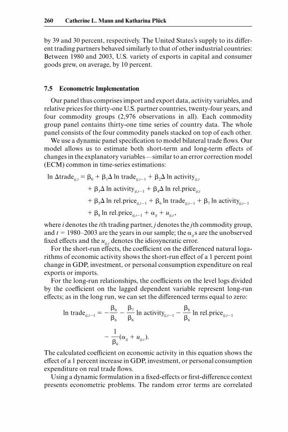
Our panel thus comprises import and export data, activity variables, andrelative prices for thirty-one U.S. partner countries, twenty-four years, andfour commodity groups (2,976 observations in all). Each commoditygroup panel contains thirty-one time series of country data. The wholepanel consists of the four commodity panels stacked on top of each other.

We use a dynamic panel specification to model bilateral trade flows. Ourmodel allows us to estimate both short-term and long-term effects ofchanges in the explanatory variables—similar to an error correction model(ECM) common in time-series estimations:

ln �tradeij,t � �0 � �1� ln tradeij,t�1 � �2� ln activityij,t

� �3� ln activityij,t�1 � �4� ln rel.priceij,t

� �5� ln rel.priceij,t�1 � �6 ln tradeij,t�1 � �7 ln activityij,t�1

� �8 ln rel.priceij,t�1 � �ij � uij,t ,

where i denotes the ith trading partner, j denotes the jth commodity group,and t � 1980–2003 are the years in our sample; the �ij s are the unobservedfixed effects and the uij,t denotes the idiosyncratic error.

For the short-run effects, the coefficient on the differenced natural loga-rithms of economic activity shows the short-run effect of a 1 percent pointchange in GDP, investment, or personal consumption expenditure on realexports or imports.

For the long-run relationships, the coefficients on the level logs dividedby the coefficient on the lagged dependent variable represent long-runeffects; as in the long run, we can set the differenced terms equal to zero:

ln tradeij,t�1 � � � ln activityij,t�1 � ln rel.priceij,t�1

� (�ij � uij,t ).

The calculated coefficient on economic activity in this equation shows theeffect of a 1 percent increase in GDP, investment, or personal consumptionexpenditure on real trade flows.

Using a dynamic formulation in a fixed-effects or first-difference contextpresents econometric problems. The random error terms are correlated

1��6

�8��6

�7��6

�0��6


both with the differences and the level of the lagged dependent variable,thus biasing the results for the coefficients. Arellano and Bond (1991) andBlundell and Bond (1998) propose an estimation method that instrumentsthe lagged levels of the dependent variable with the lagged differences ofthis variable and the differences of the dependent variable with its laggedlevels. Our results using these instruments and technique were poor.Wooldridge (2002, chapter 11) and Kennedy (2003, 313) discuss the chal-lenge of choosing an econometric technique in the context of dynamicpanel data estimation, and note the bias, yet greater precision, of fixed-effects estimators, as opposed to general least squares or instrumental vari-able regressions. Studies indicate that the bias induced by fixed effects isoffset when the time variable exceeds thirty observations. Our time series istwenty-four years, and we proceed.18

7.6 Results and Discussion

This section discusses the findings of the econometric exercise. We wishto compare estimated coefficients constrained over the whole panel versusunconstrained over several different dimensions: commodity decomposi-tion; GDP versus alternative activity variables; and industrial versus de-veloping countries.

7.6.1 Benchmark Regression and Matched Expenditure versus GDP

For the first comparison to previous research, we use the thirty-one-country and four-commodity whole panel with country- and commodity-fixed effects to run a benchmark regression for U.S. imports and U.S. ex-ports. An F-test of the constrained whole panel against the unconstrainedcountry- and commodity-fixed effects panel rejects the null hypothesis thatthe constrained and unconstrained regressions are the same. Table 7.3presents short-run and long-run estimates for the elasticity estimates forincome and for relative prices from representative previous work. Waldtests (see note to table 7.3) test the null hypothesis that the short-run andthe long-run coefficients are the same. Generally, the null is rejected for theactivity variable. For relative prices, the null is rejected for exports but notfor imports.

The first question is how our elasticities estimated using our thirty-one-country and four-commodity panel and using GDP as the measure of eco-

nomic activity compare with previous research. Our income elasticities for


18. Ideally, one might try to estimate this panel using a vector error correction model(VECM) suited for dynamic panel data estimation—these techniques go beyond the scope ofthis paper (see, for example, Beck [2001]; Schich and Pelgrin [2002]; and Smith [2000] for es-timation of long and wide panels). In future work, it makes sense to try to generate the coin-tegrating vector explicitly using panel dynamic ordinary least squares (Mark and Sul 2002;Mark, Ogaki, and Sul 2003) and implement the result in a panel ECM.

Tab

le 7

.3E

stim

ates

for

activ

ity

and

rela

tive

pric

e el

asti

citi

es fo

r U

.S. e

xpor

ts a

nd im

port

s

Exp

orts

Impo

rts

Lev

el o

f R

elat

ive

Rel

ativ

e P

revi

ous

rese

arch

Dat

a pe

riod

Met

hod

disa

ggre

gati

onpr

ice

Act

ivit

ypr

ice

Act

ivit

y

Pre

vious

rese

arc

h

Hou

thak

ker

and

Ann

ual 1

951–

66O

LS

Goo

ds a

nd s

ervi

ces

–1.5

10.

99–1

.03

1.68

Mag

ee (1

969)

1.8∗

∗(S

R)

–0.1

(SR

)1.

0∗∗

(SR

)–0

.5∗∗

∗(S

R)

0.8∗

∗∗(L

R)

–0.3

∗∗∗

(LR

)1.

8∗∗∗

(LR

)H

oope

r, Jo

hnso

n, a

nd

Qua

rter

ly 1

956–

96E

CM

(SR

);

Goo

ds a

nd s

ervi

ces

–1.5

∗∗∗

(LR

)M

arqu

ez (2

000)

Joha

nsen

(LR

)W

ren-

Lew

is a

nd

Qua

rter

ly 1

980–

95E

CM

(SR

);

Goo

ds–0

.96

(SR

)1.

12 (S

R)

–0.3

82.

43 (S

R)

Dri

ver

(199

8)Jo

hans

en (L

R)

–0.6

5 (S

R)

1.21

(LR

)–0

.18

2.36

(LR

)

Our

study

GD

P a

s in

com

eaA

nnua

l 198

0–20

03C

ount

ry- a

nd

Pan

el o

f 4 c

ateg

orie

s –0

.07∗

∗(S

R)

2.79

∗∗(S

R)

–0.1

7 (S

R)

4.11

∗∗(S

R)

com

mod

ity-

fixed

of

goo

ds–0

.2∗∗

(LR

)1.

44∗∗

(LR

)–0

.28

(LR

)2.

22∗∗

(LR

)eff

ects

, dyn

amic

–0

.03∗

(SR

)0.

58∗∗

(SR

)–0

.09

(SR

)1.

00∗∗

(SR

)pa

nel

Mat

ched

exp

endi

ture

–0

.09

(LR

)1.

19∗∗

(LR

)0.

10 (L

R)

1.63

∗∗(L

R)

and

mat

ched

pri

cesb

No

tes:

SR �

shor

t run

; LR

�lo

ng r

un; E

CM

�er

ror

corr

ecti

on m

odel

; OL

S �

ordi

nary

leas

t squ

ares

.a I

mpo

rts:

Nul

l rej

ecte

d fo

r G

DP

as

inco

me;

not

rej

ecte

d fo

r re

lati

ve p

rice

s. E

xpor

ts: N

ull r

ejec

ted

for

GD

P a

s in

com

e; n

ull r

ejec

ted

for

rela

tive

pri

ces.

bIm

port

s: N

ull r

ejec

ted

for

“act

ivit

y”; n

ot r

ejec

ted

for

rela

tive

pri

ces.

Exp

orts

: Nul

l rej

ecte

d at

1 p

erce

nt le

vel f

or “

acti

vity

”; n

ull r

ejec

ted

at 1

0 p

erce

nt le

vel o

f sig

-ni

fican

ce fo

r re

lati

ve p

rice

s.∗∗

∗ Sig

nific

ant a

t the

1 p

erce

nt le

vel.

∗∗Si

gnifi

cant

at t

he 5

per

cent

leve

l.∗ S

igni

fican

t at t

he 1

0 p

erce

nt le

vel.

both exports and imports are higher in the short run but are similar to thelong-run estimates that come from regressions run over sample periodsstarting from the 1980s, such as Wren-Lewis and Driver (1998). Our priceelasticities are generally lower than comparable studies, particularly on theexport side and often are not significant. This may be a result of the con-struction of our relative price index using the GDP deflator for all the cat-egories of trade. (Note that this is not the deflator we construct for subse-quent regressions, where we instead use matched trade price and deflators.)

Changing from the workhorse model specification to matched expendi-

ture as the measure of economic activity and matched prices makes a largedifference to the estimated income elasticities. Both the short-run andlong-run elasticities are much lower (with the short-run coefficients almosttoo low) and the long-run coefficients close to the theoretical priors basedon constant share of trade in expenditure of about 1.0. This suggests thatthe GDP variable may not be the correct measure of economic activity thatdrives trade flows.

With respect to relative prices, although the regressions with matchedexpenditure also incorporate greater richness with regard to the relativeprices (as discussed in the data section), the significance level of relativeprices does not improve in this panel specification of the four-commoditymodel.

Finally, and to be further discussed in the following, we find that the va-riety variable is statistically significant in the regressions for imports andexports implemented with matched expenditure and matched prices butnot for the export regression using GDP as the measure of activity and theGDP deflators in the measure of relative prices.

In sum, a key finding is that although the Houthakker-Magee asymme-try (in estimated elasticity of trade with respect to measures of economicactivity) persists both in the short and long run, the magnitude of theasymmetry is dramatically smaller than with the benchmark specificationof the workhorse model. Matched expenditure, matched prices, and vari-ety appear to play a key role in reducing the asymmetry of estimated elas-ticities of trade with respect to economic activity.

7.6.2 Disaggregating by Product Categories

Given that the commodity-by-country composition of trade haschanged, in some cases dramatically, do the coefficients on economic ac-tivity, relative prices, and variety vary across product categories? Table 7.4presents regressions by commodity group with country-fixed effects. An F-test of the constrained whole panel with country-fixed effects versus the un-constrained panel with country-fixed effects rejects the null hypothesis thatthe constrained and unconstrained regressions are the same. Wald tests ingeneral reject the null hypothesis that the short-run and long-run coeffi-cients are the same on the matched expenditure variable but do not reject


Tab

le 7

.4R

egre

ssio

ns b

y co

mm

odit

y gr

oup

wit

h co

untr

y fix

ed e

ffec

ts

Exp

orts

Impo

rts

Rel

ativ

e M

atch

ed

Var

iety

R

elat

ive

Mat

ched

V

arie

ty

Lev

el o

f dis

aggr

egat

ion

(R2 M

, R2 X

)pr

ice

expe

ndit

ure

cate

gori

espr

ice

expe

ndit

ure

cate

gori

es

Exp

endi

ture

and

mat

ched

pri

ces

Cap

ital

goo

ds (0

.16,

0.3

8)–0

.021

(SR

)0.

79∗∗

(SR

)4.

66∗∗

–0.2

5 (S

R)

0.48

∗∗(S

R)

1.74

∗∗0.

012

(LR

)0.

88∗∗

(LR

)1.

56∗

(LR

)1.

54∗∗

(LR

)C

onsu

mer

goo

ds (0

.18,

0.3

2)–0

.02

(SR

)0.

713∗

∗(S

R)

0.16

–0.4

0∗(S

R)

3.73

∗∗(S

R)

–0.2

10.

07 (L

R)

1.37

∗∗(L

R)

3.64

(LR

)1.

69∗∗

(LR

)A

utos

and

par

ts (0

.20,

0.2

6)–0

.07

(SR

)1.

03∗∗

(SR

)0.

92∗

0.48

(SR

)9.

01∗∗

(SR

)0.

54–0

.3∗

(LR

)1.

13∗∗

(LR

)1.

35 (L

R)

2.21

∗∗(L

R)

Ann

ual 1

980–

2003

ISM

-ex

(0.2

6, 0

.31)

0.01

(SR

)0.

35∗∗

(SR

)0.

99–0

.13

(SR

)1.

03∗∗

(SR

)0.

52∗

0.02

(LR

)0.

94∗∗

(LR

)1.

36 (L

R)

0.64

∗∗(L

R)

Pan

el o

f 4 c

ateg

orie

s of

goo

ds (0

.25,

0.1

4)–0

.03∗

∗∗(S

R)

0.58

∗∗(S

R)

0.91

∗∗–0

.17

(SR

)1.

00∗∗

(SR

)0.

70∗∗

–0.0

9 (L

R)

1.09

∗∗(L

R)

0.16

(LR

)1.

40∗∗

(LR

)

No

tes:

SR �

shor

t run

; LR

�lo

ng r

un. W

ald

Tes

t: N

ull h

ypot

hesi

s th

at S

R a

nd L

R a

re th

e sa

me.

Aut

os—

Impo

rts:

inco

me

coeffi

cien

ts r

ejec

t; p

rice

s no

t rej

ect.

Exp

orts

: inc

ome

coeffi

cien

ts r

ejec

t; p

rice

s re

ject

at 5

per

cent

leve

l. C

apit

al g

oods

—Im

port

s: in

com

e co

effici

ents

rej

ect,

pri

ces

not r

ejec

t. E

xpor

ts: i

ncom

e co

effi-

cien

ts r

ejec

t, p

rice

s no

t re

ject

. Con

sum

er g

oods

—Im

port

s: in

com

e co

effici

ents

rej

ect,

pri

ces

not

reje

ct. E

xpor

ts: i

ncom

e co

effici

ents

rej

ect,

pri

ces

not

reje

ct. I

n-du

stri

al s

uppl

ies

and

mat

eria

ls, e

xclu

ding

oil

(ISM

-ex)

—Im

port

s: in

com

e co

effici

ents

rej

ect,

pri

ces

not

reje

ct. E

xpor

ts: i

ncom

e co

effici

ents

rej

ect,

pri

ces

not

re-

ject

.∗∗

∗ Sig

nific

ant a

t the

1 p

erce

nt le

vel.

∗∗Si

gnifi

cant

at t

he 5

per

cent

leve

l.∗ S

igni

fican

t at t

he 1

0 p

erce

nt le

vel.

the null hypothesis that the short-run and long-run relative price coeffi-cients are the same (excepting that the null is rejected at the 5 percent levelfor auto exports).

Comparing the elasticities on matched expenditure and variety acrossthe commodity panels: for exports, the long-run elasticities of autos, capi-tal goods, and consumer goods are greater than the short-run elasticities,as expected. For imports, differences in estimated expenditure elasticitiesare substantial across the disaggregated commodities groups. Comparingthe short-run and the long-run estimates, the short-run cyclical respon-siveness of trade with respect to matched economic activity exceeds thelong-run responsiveness for U.S. imports of consumer goods and autosand auto parts, but this is not in evidence for capital goods. The situationof short-run exceeding long-run elasticities is consistent with the oft-discussed unsustainability of the trajectory of the U.S. trade deficit (Mann2005). Whereas most of the estimates make sense and are of plausible mag-nitudes, those for autos seem unreasonable, particularly the short-run es-timate. Based on this analysis that disaggregation of product categories isstatistically relevant for understanding the drivers of trade flows, our fu-ture program of work will allow the countries included in each product cat-egory to vary as we will no longer require the uniform panel.

7.6.3 Disaggregating Industrial and Developing Countries by Product Group

Not only has the commodity composition of trade changed but there hasalso been a significant change, particularly evident for imports, in thecomposition of U.S. trade with the industrial versus developing coun-tries. Moreover, apropos our implementation using matched expenditureand trade prices, exchange rate regimes and sources of economic growthmay differ between industrial and developing countries. Are differences ob-served in the estimated activity and relative price coefficients between in-dustrial and developing countries and across product groups? (tables 7.5and 7.6). F-tests of regressions including country-fixed effects reject thenull hypotheses that the industrial and developing countries regressionsare the same for each of the four product groups. Wald tests of the null hy-pothesis that short-run and long-run coefficients are the same are as noted.

The following summarizes key aspects of the tables:

• With respect to relative prices: The relative price coefficient is of thecorrect sign and significant for imports of consumer goods and capi-tal goods from industrial countries; it is significant and of the correctsign for all product categories of exports. This is in contrast to the es-timates that constrained the relative price coefficient to be the same forindustrial and developing countries and that resulted in poorly esti-mated coefficients.


Table 7.5 Import regressions using a dummy variable for industrial trading partner withcountry-fixed effects

Matched expenditure Relative priceVariety

Level of Industrial Developing Industrial Developing categories, disaggregation country country country country 1980–2003

Capital goods 1.29∗∗ (SR) –0.24∗ (SR) –0.31 (SR) –0.20 (SR)0.78∗∗ (LR) 3.12∗∗ (LR) –0.71∗∗ (LR) 5.01∗∗ (LR) 1.42∗∗3.52a (SR) 4.156∗∗ (SR) –1.35∗∗ (SR) 0.86∗∗∗ (SR)

Consumer goods 1.32a (LR) 1.96∗∗ (SR) –4.34∗∗ (LR) 14.34∗∗ (SR) –0.198.16∗∗ (SR) 9.72∗∗∗ (SR) 0.72 (SR) 2.26∗ (SR)

Autos and parts 1.59∗∗ (LR) 3.53∗∗ (LR) –1.71 (LR) 6.88 (LR) 0.321.52∗∗ (SR) 0.97∗∗ (SR) –0.29 (SR) 0.16 (SR)

ISM-ex 0.26 (LR) 1.47∗∗ (LR) 1.97 (LR) 0.86 (LR) 0.17

Notes: SR � short run; LR � long run. Wald Test: Null hypothesis that LR and SR are the same. Cap-ital goods—Expenditure for both groups rejects the null. Consumer goods—Relative price for bothgroups rejects the null. Autos—Expenditure for developing countries rejects the null. Industrial suppliesand materials, excluding oil (ISM-ex)—Expenditure for developing countries rejects the null and for in-dustrial country at the 10 percent level.aDummy for industrial countries is not significant.∗∗∗Significant at the 1 percent level.∗∗Significant at the 5 percent level.∗Significant at the 10 percent level.

Table 7.6 Export regressions using a dummy variable for industrial trading partner withcountry-fixed effects

Matched expenditure Relative priceVariety

Level of Industrial Developing Industrial Developing categories, disaggregation country country country country 1980–2003

Capital goods 0.67∗ (SR) 0.79∗∗ (SR) –0.38∗∗ (SR) –0.014 (SR)0.70∗∗∗ (LR) 0.94∗∗ (LR) 0.12 (LR) 0.013 (LR) 5.2∗∗0.45∗∗ (SR) 0.69∗∗ (SR) –0.45∗∗ (SR) 0.014 (SR)

Consumer goods 1.09∗∗ (LR) 1.64∗∗ (SR) –0.58∗ (LR) 0.022 (LR) –0.121.19∗∗∗ (SR) 1.41∗∗ (SR) –0.922∗∗ (SR) 0.043 (SR)

Autos and parts 0.66∗∗∗ (LR) 1.22∗∗ (LR) –1.55∗∗ (LR) –0.19 (LR) 0.790.32a (SR) 0.37∗∗ (SR) –0.02 (SR) 0.01 (SR)

ISM-ex 0.81∗∗ (LR) 1.46∗∗ (LR) –1.18∗∗ (LR) –0.26 (LR) –0.46

Notes: SR � short run; LR � long run. Wald Test: Null hypothesis that SR and LR are the same. Cap-ital goods—Expenditure for developing countries rejects the null. Consumer goods—Expenditure fordeveloping countries reject (1 percent level); expenditure industrial countries reject (5 percent level); rel-ative prices industrial countries reject (1 percent level). Autos—Expenditure for developing countriesand relative prices for industrial countries reject the null. Industrial supplies and materials, excluding oil(ISM-ex)—Expenditure for both groups reject; relative prices for industrial countries reject (5 percentlevel).aDummy for industrial countries is not significant.∗∗∗Significant at the 1 percent level.∗∗Significant at the 5 percent level.∗Significant at the 10 percent level.

• With respect to activity: The elasticity for U.S. capital goods exports toindustrial countries does not differ significantly from that to develop-ing countries, but U.S. capital goods imports from industrial countriesis more responsive in the short run and less responsive in the long runto U.S. activity than imports from developing countries. The U.S. con-sumer goods exports to industrial countries respond differently to for-eign activity in those high-income countries as compared with theresponse to activity in the developing countries. On the other hand,there is no difference in elasticity of U.S. consumer goods imports withrespect to source country.

What does all this add up to in the context of the recent evolution of theU.S. trade deficit? First, with respect to capital goods imports and exports,changing relative prices in industrial countries, and net trade, these coeffi-cients are consistent with a story that dollar appreciation has, ceterisparibus, dampened capital goods exports and encouraged capital goodsimports from the industrial countries. The depreciation of the dollaragainst these same currencies since 2002, and the somewhat higher pass-through of that exchange rate change vis-à-vis at least the euro19 may, ce-teris paribus, change the trajectory of the trade deficit in capital goods(presented in figure 7.1). But, to the extent that an increasing share of thesegoods come from developing economies, any dollar depreciation may haveless of an effect to reduce capital goods imports or expand capital goodsexports to developing countries, given the lack of significance in the esti-mated coefficient for relative prices of capital goods for developing coun-tries.20

Second, with respect to changing investment activity, these coefficientsare consistent with a story that robust U.S. investment demand has en-couraged imports of capital goods with a relatively higher elasticity,whereas slower investment growth abroad (both in the industrial and thedeveloping world) has tended to yield slower growth in capital goods ex-ports.

Third, the fact that the variety effect is smaller for imports than for ex-ports suggests that variety importantly underpins U.S. capital goods ex-port growth, which is consistent with Schott (2004). Put together, the dete-rioration of net trade in capital goods comes from relatively more robust


19. The U.S. import prices from the European Union have risen about 14 percent since thepeak of the dollar in February 2002. This represents more than a 25 percent pass-through ofthe euro appreciation into U.S. import prices. Import prices from Japan, on the other hand,have stayed stable since early 2002, in spite of a more than 25 percent appreciation of the yenagainst the dollar (Bureau of Labor Statistics)—while this limited pass-through is no doubtdue in part to deflation in Japan that cannot be the only story.

20. The large positive and significant long-run coefficient for relative price of capital goodsimports from developing countries suggests another missing variable or that the variety vari-able needs additional work.

U.S. investment with a relatively higher elasticity, a dollar appreciationparticularly against the industrial countries where relative prices are esti-mated significantly, and significant increases in global supply-cum-variety.

For consumer goods, the story is somewhat different not only because theestimated U.S. consumer demand elasticity is so high in the short-run butalso because relative prices are significant and rather high for productsfrom the industrial countries. First, with respect to changing relative prices

in industrial countries and net trade in consumer goods, these coefficientsare consistent with a story that dollar appreciation has, ceteris paribus,hurt consumer goods exports to industrial countries and, particularlygiven the higher relative price elasticity, encouraged consumer goods im-ports from industrial countries. The depreciation of the dollar againstthese same currencies since 2002, and the somewhat higher pass-throughof that exchange rate change vis-à-vis at least the euro may, ceteris paribus,reduce the net trade deficit in consumer goods (presented in figure 7.1).But, to the extent that an increasing share of consumer goods come fromdeveloping economies, any dollar depreciation may have less of an effect toreduce consumer goods imports, given the poorly estimated coefficient forrelative prices of consumer goods from developing countries.21

Second, with respect to consumer demand growth, variety, and net trade,the coefficients are consistent with a story that relatively more robust U.S.consumer demand along with a very high short-run cyclical demand elas-ticity has encouraged imports of consumer goods and autos from all trad-ing partners well in excess of the foreign demand for U.S. exports of con-sumer goods. Surprisingly, global supply-cum-variety does not appear tobe a relevant determinant of trade in consumer goods. Put together, thedeterioration of net trade in consumer goods comes from relatively strongU.S. consumer demand growth with a relatively higher short-run elasticity,as well as dollar appreciation (with greater imports of luxury, price-sensitive goods from industrial countries, and reduced exports of similarlyprice-sensitive goods to industrial countries).

7.6.4 Summary of Findings

The paper prepared new estimates of the elasticity of U.S. trade flows us-ing bilateral trade data for thirty-one countries, using different measures ofexpenditure and including alternative measures of global supply and vari-ety. We examine four categories of goods based on the BEA’s end-use clas-sification system—autos, ISM-ex, consumer goods, and capital goods. Weconsider whether industrial and developing countries differ in their elas-ticities.


21. The large positive and significant long-run coefficient for relative price of consumergoods imports from developing countries suggests another missing variable or that the vari-ety variable needs additional work.

1. Using expenditure matched to commodity group rather than GDP asthe measure of income significantly reduces the Houthakker-Magee asym-metry in the long-run estimates and yields far more plausible values forthese income elasticities.

2. Short-run estimates of U.S. consumer goods imports with respect tomatched economic activity exhibit very high cyclical elasticity, which isconsistent with the unsustainability of the trajectory of the trade deficit.

3. The four product categories behave significantly differently from anaggregated panel.

4. Global supply-cum-variety is a significant variable, particularly forcapital goods.

5. Industrial and developing countries have different income and rela-tive price elasticities for these four product groups. In particular, when in-dustrial countries are distinguished from developing countries, the esti-mated coefficients for relative prices for industrial countries are the correctsign, significant, and of plausible values.

6. We also investigated whether U.S.-China trade is significantly differ-ent than industrial country or developing country trade. The results arenot conclusive.22

7.7 Implications and Direction for Further Work

7.7.1 Do Changing Trade Shares Change Trade Elasticities?

The results indicate that industrial and developing countries differ intheir elasticities of economic activity and relative price. The shares of thesetwo groups in trade have changed over time, in particular within productcategories for imports. When elasticities for economic activity from the re-gression that splits the panel into four product categories and allows theelasticities to vary across the industrial and developing countries (tables7.5 and 7.6) are reaggregated using the annual trade weights of these twogroups and for the four product categories in U.S. trade, we conclude thatthe long-run expenditure elasticity of U.S. imports rises from 1980 to 2003.These results imply that the assumption of a constant elasticity of U.S. im-ports with respect to U.S. economic activity may have to be rejected andthat projections of U.S. imports based on the constant elasticity assump-tion may be flawed. No similar trend is apparent for the expenditure elas-


22. For a number of reasons, we might expect China to be different from other countries inthis specification of U.S. dynamic trade. China’s trade shares changed the most. Its net tradedeficit is on the steepest trajectory. Its variety increased the most. Its exchange rates havechanged the least. Table 6 in Mann and Plück (2005) reports regression results investigatingwhether China is appreciably different from the rest of the world in the consumer goods andcapital goods categories. The bottom line is that the picture is mixed in terms of short-run ver-sus long-run effects. The very large long-run estimates on U.S. economic activity are consis-tent with the graphical evidence but arguably could not persist.


Table 7.7 Summary of in-sample predictive performance (billions of U.S. dollars)

Matched expenditure, GDP as income and variety, and industrial aggregate trade flows

country dummies (from table 7.3)

Total error, 1998–2003 Imports Exports Imports Exports

Using whole-panel estimates 386 134 198 234Using good-specific elasticities

Consumer goods 172.99 0.89 20.43 23.27Capital goods –73.16 110.50 –0.15 124.83Autos 273.2 28.99 97.91 42.04Industrial supplies and materials,

excluding oil 12.94 –6.69 106.52 20.41

ticity for exports, which is consistent with the observation that countryshares have changed less.23

7.7.2 Do These New Elasticities Predict Better?

Research using the workhorse model often addresses the tension betweenthe theoretical plausibility of the estimated elasticities, specifically theHouthakker-Magee asymmetry, and the affirmed excellence of these simpleequations to predict U.S. exports and imports in the short and mediumterms. By using matched expenditure and trade prices and by disaggregat-ing product groups and industrial versus developing countries, we reducethe Houthakker-Magee asymmetry, but do we “do better” at prediction?

We examine this question by comparing in-sample predictive performanceof two alternative models, estimating the models from 1980 to 1997, and thenrunning the model forward from 1998 to 2003 using the short-run and long-run estimated coefficients for matched expenditure and relative prices and theactual values from the right-hand-side variables. We compare the actual withthe predicted values in each year and sum the difference as the total error(table 7.7). The horse race is between the benchmark model that uses GDPand aggregated trade (from table 7.3)—a formulation that many forecasterswould use because they are interested in aggregate exports and imports; andthe matched expenditure model, with variety, with four separate productgroups, and with industrial country dummies (from tables 7.5 and 7.6).

The bottom line in terms of predicted performance is the sum of the in-sample predictive errors. For total exports, our country-commodity disag-gregated estimates better predict exports compared with the simple model.For total imports, even though we obtain more plausible values for the long-run elasticities, our predictions are poor compared with the benchmarkmodel that uses U.S. GDP as the measure of expenditure because the short-

23. See discussion and presentation of the data, particularly figure 3 in Mann and Plück(2005).

run elasticities are so high, particularly for consumer goods and autos. Ourresults address the finding that surprised Houthakker and Magee (1969) intheir original study: the very low income elasticities for U.S. exports. Our es-timations suggest that these elasticities might in fact be closer to those ofother industrial countries. But we have more work to do on the import sideto estimate elasticities that meet theoretical norms and also predict well.

Does our matched expenditure model do equally well (or poorly) in thefour commodity groups? We examined each of the four product groupscomparing the model results for the matched expenditure, variety, andindustrial-country dummies with the simple model that uses GDP as thedriver of trade. (See table 7.7.) Within product groups, auto trade and con-sumer goods imports are particularly poorly explained in-sample by thenew disaggregated model. But all the export categories are better predictedin-sample by the matched expenditure and variety model than when GDPis used as the measure of economic activity. Hence, future work should fo-cus on narrowing the country group for autos and reestimating the equationfor consumer goods, including augmenting the drivers of economic activity(beyond personal consumption expenditures to add a wealth variable forexample) and recalculating the variety variable with more detailed data.

7.7.3 “What If” U.S. Spending Slows and Foreign Spending Booms?

In recent policymaker confabs such as the G8, it has been common tocall for increased U.S. savings and greater foreign growth as well as moreflexibility in exchange rate regimes.24 Suppose the United States saves moreand growth abroad increases over the next several years to 2007 [2006?]?How much would the U.S. trade deficit be different from a scenario wheregrowth is as projected by Consensus Economics Forecasts, a well-knowneconomic forecasting group?

The assumptions for real consumption and investment growth for oursample of countries from Consensus Economics Forecasts and our estimatedelasticities are the starting points for illustrative scenarios for how U.S. tradedeficit adjustment might take place for 2007 [2006?] (figure 7.3 and table 7.8). Given the estimated short-run and long-run elasticities, the Consensus

Economics Forecasts, and no change in the exchange value of the dollar (frommid-2005), the real nonoil trade deficit in 2006 would be about $725 billion.

A rest-of-world investment boom and a rest-of-world consumptionboom (as quantified in table 7.8, where boom is defined as the average highvalue for consumption or investment growth over the 1980 to 2003 period)yield some narrowing of the U.S. trade deficit. But because most of ourcapital goods exports go to mature industrial markets, whose averagebooms are modest, and because the short-run and long-run elasticities forexports are relatively low, our capital goods exports do not increase thatmuch. And because the share of consumption goods in U.S. exports is rel-


24. This section draws on Mann (2006).

Fig. 7.3 Projected real trade deficit (ex. Oil), using commodity-specific elasticityestimates, billions of U.S. dollarsSource: Authors’ calculations using regression estimates and forecasts for country investmentand personal consumption expenditure from Consensus Economics Forecasts, August 2005(http://www.consensusforecasts.com); Macroadvisers’ Economic Outlook; United NationsComtrade database; Macroadvisers forecast for real X and M growth are generated frommacroadviser’s forecast from June 22, 2005 (volume 23, number 5).

atively small, booming consumption abroad does little to improve thetrade account. Overall, global consumption and investment booms do notplay a very large role in narrowing the trade deficit in the short term be-cause the geographical and commodity patterns of trade on the export sidehave been remarkably stable for twenty-five years. Over the longer term,however, as the long-term elasticities for exports are larger than the short-run elasticities, sustained foreign growth could have a larger impact on thetrajectory of the U.S. trade deficit.

In contrast, investment and consumption slowdowns in the United States(compared to historical cycles from the 1980 to 2003 period) would yield aquick stabilizing of the real trade deficit. This is because consumption goodsand autos are a large share of imports, and both have high estimated short-runelasticity of demand. The consumption slow-down assumed for the UnitedStates is modest by historical standards of the last twenty-five years but, nev-ertheless, is outside recent experience and therefore likely to be painful.25

What about a role for the exchange value of the dollar? Based on our es-timates, the exchange rate plays an important role in expenditure switchingfor trade with industrial countries, but has little empirical significance for

25. See also Truman (2005) for a similar conclusion.

exports to or imports from developing countries, for which real exchangerates have moved relatively little.

Our results are consistent with the findings of Freund and Warnock(chap. 4 in this volume), and Faruqee, Laxton, Muir, and Pesenti (chap. 10in this volume). Freund and Warnock conclude that adjustments to con-sumption-driven current account deficits require significantly steeper ex-change rate depreciation and thus more pain than adjustments to tradedeficits that have financed private investment. Faruqee et al. determine thata loss of foreign appetite for U.S. assets (reflected in a dollar depreciation)and a consolidation of the U.S. fiscal position have a much larger impacton the current account deficit than do structural reforms in Japan and Eu-rope. To the extent that a consolidation in the U.S. fiscal position tookplace via a sun-setting of the income tax cuts, then fiscal consolidation anddemand for consumer goods imports would be more clearly linked.

On the other hand, our findings that the relative price elasticities are sig-nificant, but not large, and are limited to industrial countries, implies achallenge to the mechanism for adjustment emphasized in Obstfeld andRogoff (chap. 9 in this volume). Their mechanism for adjustment dependson the relative price signal shifting resources between traded and non-traded sectors. Our relative price signal appears to play a more modest rolein directing trade flows.

7.7.4 Conclusions and Further Work

These new elasticities yield insights into the sources of the widening ofthe U.S. trade deficit and help to understand the nature of global competi-tion and how it is impacting broad sectors of the U.S. economy.


Table 7.8 Assumptions for growth scenarios in figure 7.3

Average for “boom” in ROW/Consensus forecasts (real Add percentage “realistic slowdown” for the U.S. growth, percentage points) 2005 2006 points to achieve: (based on 1980–2003 data)

Gross fixed capital formation

Europe and Japan 3.5 3.7 5.0 8.4Other industrial countries 7.4 7.2 7.0 14.8Developing countries 9.2 7.5 1.0 9.9United States 8.8 7.5 –13.0 –6.0

Personal consumption expenditures

Europe and Japan 1.3 1.7 7.0 8.3Other industrial countries 3.1 3.1 5.0 8.3Developing countries 4.9 4.4 11.0 15.2United States 3.5 3.1 –3.0 0

Source: Authors’ calculations using regression estimates and forecasts for country investment andpersonal consumption expenditure from Consensus Economics Forecasts, August 2005 (http://www.consensusforecasts.com).Note: ROW � Rest of the world.

The differences in demand elasticities for consumer goods versus forother product categories—with consumer goods more responsive to con-sumption patterns in the United States—yields insights into how robustU.S. consumer demand through trending lower household saving rates, asaugmented by higher stock-market valuation in the 1990s and residentialhousing values and tax cuts in the 2000s, contributes to widening the con-sumer goods share of the trade deficit.

The differences in relative price elasticities between the industrial anddeveloping countries—with relative prices significant and of correct signfor industrial countries but not for developing countries—yields insightsinto how certain exchange rate regimes, pricing-to-market behavior, orother factors more prevalent to developing country exporters mute theprice signal, which is consistent with recent work on disaggregate pass-through (Campa and Goldberg 2004; Marazzi et al. 2005).

The evidence from this analysis suggests that the matched-expendituremodel for exports, disaggregated across commodity groups and incomeclass (industrial versus developing), is worth continued investigation. Notonly do the elasticities have more plausible values, particularly in the long-run, but also the equation performs better in-sample than the benchmarkmodel for exports. Simultaneous specification with an equation for relativeprices warrants consideration.

For imports, the matched-expenditure disaggregated model yields moreplausible values for trade elasticities in the long run. However, the in-sample predictive performance is much worse than for the benchmarkmodel because the short-run elasticities are very high. To understand thefactors underpinning robust U.S. imports of consumer goods and autos, inparticular, requires additional work. Future work will focus on narrowingthe country set for trade in autos and investigating a more detailed variablefor variety for consumer goods as well as incorporating a wealth variableinto the consumption goods equation.

Going forward, these new elasticities have implications for demandmanagement and exchange rate policies. In particular, slack U.S. exportsappear importantly related to slack consumption and investment abroadand low long-term growth prospects in the major markets for U.S. exports,which have been masked by measures of GDP that incorporate net exportsto the United States. On the other hand, factors beyond strong U.S. con-sumer demand or love of variety are bolstering U.S. imports of consumergoods. Different relative price elasticities between the industrial and devel-oping countries suggest long-run implications for U.S. trade of certain ex-change rate regimes. Exchange rate regimes that limit the transmission ofrelative price signals appear to have been important in the past. A changein these regimes will be an important part of the change in the trajectory ofthe U.S. trade deficit going forward.


App

endi

x

Tab

le 7

A.1

Defi

niti

on o

f pro

xy e

nd-u

se c

omm

odit

y gr

oups

Aut

osC

apit

al g

oods

Con

sum

er g

oods

Indu

stri

al s

uppl

ies

and

mat

eria

ls

No

te:

Thi

s ta

ble

is c

onst

ruct

ed u

sing

the

Stan

dard

Int

erna

tion

al T

rade

Cla

ssifi

cati

on (S

ITC

), R

evis

ion

2 (U

nite

d N

atio

ns 1

975)

.

7810

–784

9, 7

861,

786

9: ro

ad v

ehic

les

and

part

s ex

cept

mot

orcy

cles

and

bicy

cles

and

thei

r pa

rts.

625

1, 6

252:

tire

s fo

r ro

ad v

ehic

les.

6253

: tir

es fo

r ai

rcra

ft. 7

1–75

: hea

vym

achi

nes

for

all i

ndus

tria

l sec

tors

and

agri

cult

ure,

offi

ce m

achi

nes.

7641

–764

9: te

leco

mm

unic

atio

ns a

ndbr

oadc

asti

ng e

quip

men

t. 7

71–7

74,

778:

ele

ctri

cal e

quip

men

t and

elec

tron

ic e

quip

men

t. 7

911–

7938

:tr

ansp

ort e

quip

men

t oth

er th

an ro

adve

hicl

es. 8

7: la

bora

tory

and

med

ical

and

othe

r sc

ient

ific

equi

pmen

t;pr

ecis

ion

inst

rum

ents

.

1221

–122

3: to

bacc

o m

anuf

actu

red.

5411

–541

9: p

harm

aceu

tica

ls a

ndco

smet

ics.

553

0–55

43: p

erfu

mes

,so

aps

and

dete

rgen

ts. 6

121–

6129

:ar

ticl

es o

f lea

ther

and

foot

wea

r.63

54: m

anuf

actu

res

of w

ood

for

dom

esti

c us

e. 6

581–

6597

: tex

tile

an

d no

ntex

tile

furn

ishi

ng, fl

oor

cove

ring

s, r

ugs

and

othe

r ar

ticl

esm

ade

from

fabr

ic. 6

651–

6674

: ch

ina,

gla

ssw

are,

pre

ciou

s st

ones

.69

60–6

978:

hou

seho

ld it

ems

mad

e of

met

al. 7

611–

7631

: tel

evis

ions

, rad

io,

etc.

775

: hou

seho

ld a

pplia

nces

. 78

5: m

otor

cycl

es, b

icyc

les,

and

par

ts.

821:

furn

itur

e. 8

310:

trav

el g

oods

.84

–85:

app

arel

and

foot

wea

r. 88

–89:

phot

ogra

phic

equ

ipm

ent,

spe

ctac

les,

wat

ches

, pri

nted

mat

ter,

and

mis

cella

neou

s co

nsum

er g

oods

.

Cha

pter

2: c

rude

mat

eria

ls in

edib

le,

exce

pt fu

els.

Cha

pter

4: a

nim

al a

ndve

geta

ble

oils

and

wax

es. 5

1–53

:or

gani

c an

d in

orga

nic

chem

ical

s;dy

eing

, tan

ning

, and

col

orin

gsu

pplie

s. 5

51: E

ssen

tial

oils

. 56–

59:

fert

ilize

rs, e

xplo

sive

s, p

last

ics,

and

mis

cella

neou

s ch

emic

al m

ater

ials

.61

1, 6

13: l

eath

er a

nd fu

661–

664:

nonm

etal

lic m

iner

al p

rodu

cts.

r. 6

21,

628:

rub

ber.

633–

635:

woo

d an

d co

rkm

anuf

actu

res

(exc

ept 6

354

for

dom

esti

c us

e). 6

4: p

aper

and

pul

p.65

5–65

7: y

arn

and

text

iles.

67,

68:

iron

and

ste

el a

nd n

onfe

rrou

s m

etal

s.69

1–69

5, 6

99: m

anuf

actu

res

of m

etal

.77

6: s

emic

ondu

ctor

s, c

atho

des,

diod

es, p

hoto

cells

, etc

. 81:

san

itar

y,pl

umbi

ng, h

eati

ng a

nd li

ghti

ngfix

ture

s, a

nd o

ther

bui

ldin

g m

ater

ial.

References

Adler, J. Hans. 1945. United States import demand during the interwar period. TheAmerican Economic Review 35:418–30.

———. 1946. The postwar demand for United States exports. Review of EconomicStatistics 28:23–33.

Arellano, Manuel, and Stephen Bond. 1991. Some tests of specification for paneldata. The Review of Economic Studies 58:277–97.

Bayoumi, Tamim. 1999. Estimating trade equations from aggregate bilateral data.IMF Working Paper no. WP/99/74. Washington, DC: International MonetaryFund, May.

Beck, Nathaniel. 2001. Time series cross-section data. Statistica Neerlandica 55:111–33.

Blundell, Richard, and Stephen Bond. 1998. Initial conditions and moment re-strictions in dynamic panel data models. Journal of Econometrics 87:115–43.

Broda, Christian, and David E. Weinstein. 2004. Globalization and the Gains fromVariety. NBER Working Paper no. 10314. Cambridge, MA: National Bureau ofEconomic Research, February.

Campa, José Manuel, and Linda S. Goldberg. 2004. Exchange rate pass-throughinto import prices. New York: Federal Reserve Bank of New York.

Castles, Ian, and David Henderson. 2005. International comparisons of GDP: Is-sues of theory and practice. World Economics 6 (1): 55–84.

Chang, Tse Chun. 1945–1946. International comparison of demand for imports.The Review of Economic Studies 13:53–67.

Cline, William R. (forthcoming). The United States as a debtor nation. Washington,DC: Institute for International Economics.

Deardorff, Alan S., Saul H. Humans, Robert M. Stern, and Chong Xiang. 2001.Forecasting U.S. trade in services. In Services in the international economy, ed.Robert M. Stern, 53–83. Ann Arbor, MI: University of Michigan Press.

Feenstra, Robert C. 1994. New product varieties and the measurement of interna-tional prices. The American Economic Review 84:157–77.

Funke, Michael, and Ralf Ruhwedel. 2001. Product variety and economic growth:Empirical evidence for the OECD countries. IMF Staff Papers 48:225–42. Wash-ington, DC: International Monetary Fund.

Gagnon, Joseph E. 2003b. Productive capacity, product varieties, and the elastici-ties approach to the trade balance. International Finance Discussion Papers no.781. Washington, DC: Board of Governors of the Federal Reserve System.

———. 2003a. Long-run supply effects and the elasticities approach to trade. In-ternational Finance Discussion Papers no. 754. Washington, DC: Board of Gov-ernors of the Federal Reserve System.

———. 2004. Growth-led exports: Is variety the spice of trade? International Fi-nance Discussion Papers no. 822. Washington, DC: Board of Governors of theFederal Reserve System.

Goldstein, Morris, and Mohsin S. Khan. 1985. Income and price effects in foreigntrade. In Handbook of international economics Vol. 2, ed. R. W. Jones and P. B.Kenen, 1041–1105. Amsterdam: Elsevier Science.

Helkie, William L., and Peter Hooper. 1988. An empirical analysis of the externaldeficit, 1980–86. In External deficits and the dollar, the pit, and the pendulum, ed.Ralph C. Bryant, Gerald Holtham, and Peter Hooper, passim. Washington, DC:Brookings Institution.

Hooper, Peter, Karen Johnson, and Jaime Marquez. 2000. Trade elasticities for the


G-7 countries. Princeton, NJ: Princeton University, Department of Economics,International Economics Section.

Houthakker, Hendrik S., and Stephen P. Magee. 1969. Income and price elasticitiesin world trade. Review of Economics and Statistics 51:111–23.

Hummels, David, and Peter Klenow. 2004. The variety and quality of a nation’s ex-ports. The American Economic Review, forthcoming.

Kennedy, Peter. 2003. A guide to econometrics. 5th ed. Cambridge, MA: MIT Press.Krugman, Paul. 1989. Differences in income elasticities and trends in real exchange

rates. European Economic Review 33:1031–54.Krugman, Paul R., and Richard E. Baldwin. 1987. The persistence of the U.S. trade

deficit. Brookings Papers on Economic Activity, Issue no. 1:1–55. Washington,DC: Brookings Institution.

Mann, Catherine L. 1999. Is the U.S. trade deficit sustainable? Washington, DC: In-stitute for International Economics.

———. 2004. The U.S. current account, new economy services, and implicationsfor sustainability. Review of International Economics 12:262–76.

———. 2005. Breaking up is hard to do: Global co-dependency, collective action,and the challenges of global adjustment. CESifo Forum 6 (1): 16–23.

———. 2006. Current account imbalances: How will ours end? http://www.kansascityfed.org/PUBLICAT/SYMPOS/PDF/Mann2005.pdf.

Mann, Catherine L., and Katharina Plück. 2005. The U.S. trade deficit: A disag-gregate perspective. IIE Working Paper no. 05-11. Washington, DC: Institute forInternational Economics, September.

Marazzi, Mario, Nathan Sheets, Robert Vigfusson, et al. 2005. Exchange rate pass-through to U.S. import prices: Some new evidence. International Finance Dis-cussion Papers no. 833. Washington, DC: Board of Governors of the Federal Re-serve System.

Mark, Nelson C., Masao Ogaki, and Donggyu Sul. 2003. Dynamic Seemingly Un-related Cointegration Regression. NBER Technical Working Paper no. 292.Cambridge, MA: National Bureau of Economic Research.

Mark, Nelson C., and Donggyu Sul. 2002. Cointegration vector estimation bypanel DOLS and long-run money demand. Technical Working Paper no. 287.Cambridge, MA: National Bureau of Economic Research.

Marquez, Jaime. 1999. Long-period trade elasticities for Canada, Japan, and theUnited States. Review of International Economics 7 (1): 102–16.

———. 2002. Estimating trade elasticities. In Advanced Studies in Theoretical andApplied Econometrics 39. Boston: Kluwer Academic.

Sawyer, W. Charles, and Richard L. Sprinkle. 1996. The demand for imports andexports in the U.S.: A survey. Journal of Economics and Finance 20:147–78.

Schich, Sebastian, and Florian Pelgrin. 2002. Financial development and invest-ment: Panel data evidence for OECD countries from 1970 to 1997. Applied Eco-nomics Letters 9:1–7.

Schott, Peter K. 2004. Across product versus within-product specialization in in-ternational trade. The Quarterly Journal of Economics 119:647–77.

Smith, Ron P. 2000. Estimation and inference with non-stationary panel time-seriesdata. Paper prepared for the RC33 conference. 2 October, Cologne, Germany.

Stern, Robert M., Christopher F. Baum, and Mark N. Greene. 1979. Evidence onstructural change in the demand for aggregate U.S. imports and exports. Journalof Political Economy 87:179–92.

Stone, Joe A. 1979. Price elasticities of demand for imports and exports: Industryestimates for the U.S., the E.E.C., and Japan. Review of Economics and Statistics61:306–12.


Truman, Edwin. 2005. Postponing global adjustment: An analysis of the pendingadjustment of global imbalances. Institute for International Economics Work-ing Paper no. 05-6. Washington, DC: IIE.

United Nations, Department of Economics and Social Affairs, Statistical Office.1975. Standard international trade classification, revision 2. Statistical Papers,Series M No. 34/Rev. 2. New York: United Nations.

Welsch, Heinz. 1987. An aggregate import demand model for long-term projec-tions. Jahrbücher für Nationalökonomie und Statistik 203:372–89.

Wilson, John F., and Wendy E. Takacs. 1979. Differential responses to price andexchange rate influences in the foreign trade of selected industrial countries. Re-view of Economics and Statistics 61:267–79.

Wooldridge, Jeffrey M. 2002. Econometric analysis of cross-section and panel data.Cambridge, MA: MIT Press.

Wren-Lewis, Simon, and Rebecca L. Driver. 1998. Real exchange rates for the year2000. In Policy Analyses in International Economics 54. Washington, DC: Insti-tute for International Economics.

Comment Peter B. Kenen

I begin with thanks to the organizer of this conference and the authors ofthis paper—thanks to the organizer for the compliment implied by askingme to comment on a technically sophisticated paper, and thanks to the au-thors for a meticulous effort to answer some rather important questions.

There is a strong conceptual case for disaggregating trade flows, espe-cially for the United States, which trades with many countries and in manygoods. Otherwise, estimates of income and price elasticities may be badlybiased by changes in the country and commodity composition of U.S.trade. I am not sure, however, that the paper by Mann and Plück deals de-cisively with that need. They do disaggregate by commodity group, whichallows them to ask whether it is better to use different measures of eco-nomic activity for different commodity groups rather than follow the com-mon practice of using GDP for each and every group. They also distinguishbetween U.S. trade with industrial countries and with developing coun-tries. Nevertheless, their strategy and findings raise several questions.

The first question pertains to the treatment of industrial materials.Shouldn’t the demand for those goods be more responsive to changes in in-dustrial production than to changes in investment? Use of the two GDPcomponents, consumption and investment, as explanatory variables is ap-pealing; they are mutually exclusive categories, whereas industrial produc-tion may be destined for consumption or investment. Furthermore, theiruse of the two GDP components helps them to compare the trade-balance


Peter B. Kenen is a senior fellow at the Council on Foreign Relations, and the Walker Pro-fessor of Economics and International Finance Emeritus at Princeton University.

effect of a change in household consumption with the trade-balance effectof a change in business investment. Yet that comparison may be badlyflawed insofar as trade in industrial materials truly reflects the joint effectsof household and business demand for final products that embody largeamounts of industrial materials. I wonder, moreover, whether the use of in-vestment as the expenditure variable in the trade equations for industrialmaterials accounts for one of the striking results shown in table 7.4 of thepaper; this is the only case in which the expenditure coefficient in the long-run demand equation for U.S. exports exceeds the expenditure coefficientin the long-run demand equation for U.S. imports.

The second question pertains to the pooling of time series and countrydata, which constrains the price and income elasticities to be the same forthe thirty-one countries in their sample. To what extent does this blur theeffects of changes in the country composition of U.S. foreign trade? Intables 7.5 and 7.6 of their paper, Mann and Plück present results for twogroups of countries—industrial and developing countries. In a previousversion of their paper, moreover, they presented separate results for U.S.trade with China.1 It might be useful, however, to derive separate equationsfor some other countries, especially Canada and Mexico, given their verylarge trade with the United States, and to compare the resulting equationswith those for other countries or country groups. Disaggregation by coun-try or country group would be especially helpful when, as in the final partof the paper, Mann and Plück discuss the likely effects of various changesin economic conditions at home and abroad, including changes in ex-change rates. Disaggregation by country or country group would be moreuseful for this purpose than disaggregation by commodity group.

The third question pertains to the effects of omitting completely trade inoil and food. Mann and Plück had to do that, for reasons explained in theirpaper. But they should perhaps have warned their readers that the exclu-sion of oil and food may impair the comparability of their regression re-sults with those obtained by other studies. Could it perhaps help to explainwhy their results differ appreciably from those of the other three studiesshown in table 7.3—why in particular they succeed in narrowing theHouthakker-Magee asymmetry, a matter to which I return in the follow-ing.

Thus far, I have focused on what Mann and Plück did. Let me turn nowto some of the things they say, especially their quasi-normative use of theHouthakker-Magee asymmetry—the fact that, in most studies, as well asin most of their own trade equations, the income elasticity of the U.S. de-mand for imports exceeds the income elasticity of the foreign demand forU.S. exports. Citing Krugman and Baldwin (1987), they say that this find-ing is incompatible with a global long-run equilibrium:


1. See also footnote 22 to the present version.

The estimates imply that if the United States and the rest of the worldgrow at the same pace (long-run convergence), the U.S. trade deficitwould worsen, absent a trend change in relative price—which is also in-consistent with long-run equilibrium.

The Houthakker-Magee asymmetry is, as they say, manifestly inconsistentwith the long-run convergence of real incomes at constant relative prices.But a trend change in relative prices, while inconsistent with long-run con-vergence, is not inconsistent with long-run equilibrium. Recall the modelsdeveloped by Harry Johnson and others many years ago, in which equalrates of growth in output, due either to capital accumulation or technicalprogress, can lead to continuing changes in relative prices (i.e., the terms oftrade).2 It may therefore be wrong to dismiss a robust empirical findingmerely because it is inconsistent with uniform global growth at constantrelative prices. A world displaying that property would be pretty indeed,but we should not be dismayed by a world that does not display it. YetMann and Plück, while not dismayed, tend too much to use the reductionof the Houthakker-Magee asymmetry as a normative criterion—to preferempirical results in which it is smaller.

My chief concern, however, derives not from the author’s treatment ofthe Houthakker-Magee asymmetry but from their results regarding theprice elasticities of demand for U.S. exports and imports. The conventional


2. See, for example, Johnson (1959).

Fig. 7C.1 The trade balance to GDP ratio and the real dollar exchange rate,lagged two yearsSource: Chinn (2005, 11). Reprinted with permission.

wisdom holds that a reduction of the U.S. current-account deficit requiresa combination of expenditure changes and expenditure switching and thatthe latter can be achieved by dollar depreciation, which should have twoeffects—switching U.S. expenditure from traded to nontraded goods, andswitching U.S. and foreign expenditure between U.S. tradables and foreigntradables. Mann and Plück express concern about the implications of theirfindings for the efficacy of the first type of switching, but I am more con-cerned about the implications for the second type.

Consider the price elasticities shown in table 7.3 of their paper. They are,without exception, lower than the ones obtained by the earlier studieslisted in that table. The long-run price elasticities are much larger for U.S.imports of consumer goods, as shown in table 7.5 and likewise larger forU.S. imports of autos and parts (although the regression coefficient fallsshort of significance). But it is wrong-signed for industrial materials. Andall of the price elasticities for U.S. imports from the developing countriesare wrong-signed, while those for U.S. exports to developing countries intable 7.5 are not significantly different from zero.

I find it quite hard to square these results with the story told by figure7C.1, which plots the U.S. trade balance relative to GDP along with the logof the U.S. real exchange lagged two years. How can these series be soclosely correlated if the relevant price elasticities are as low as those inMann and Plück’s paper?

Finally, a policy question: given the large difference between the com-puted price elasticities for U.S. trade with industrial countries and those forU.S. trade with developing countries, are we perhaps expecting too muchfrom any future appreciation of the Asian currencies? Papers elsewhere inthis volume give good reasons for believing that the renminbi and otherAsian currencies are undervalued; the huge accumulation of foreign-exchange reserves is itself indicative. But Mann and Plück’s paper makesme wonder how much to expect from a significant appreciation of theAsian currencies and thus to repeat my previous suggestion that the au-thors look more closely at smaller country groups.

References

Chinn, Menzie D. 2005. Getting serious about the twin deficits: A Council special re-port. New York: Council on Foreign Relations Press.

Johnson, Harry G. 1959. Economic development and international trade. Nation-aløkonomisk Tidsskrift 97:252–72. Repr., in Money, trade and economic growth,ed. H. G. Johnson, 75–103.

Krugman, Paul R., and Richard Baldwin. 1987. The persistence of the U.S. tradedeficit. Brookings Papers on Economic Activity, Issue no. 1:1–43. Washington,DC: Brookings Institution.


understanding the u.s. trade deficit: a disaggregated perspective

Documents