understanding real estate math - affordable real · pdf fileunderstanding real estate math ......
TRANSCRIPT

Understanding
Real Estate
Math
Presented by:

This page intentionally left blank.

UUNNDDEERRSSTTAANNDDIINNGG
RREEAALL EESSTTAATTEE
MMAATTHH MMCCEE
Published in the United States of America By: State Continuing Education/CE Source LLC
1.800.943.5573 www.cesource.com
Copyright 2015: State Continuing Education/CE Source LLC. All rights reserved. No part of this publication may be reproduced, stored in a retrieval system, or transmitted in any form or by any means, electronic, mechanical, photocopying, recording or otherwise, without the prior written permission of the Publisher.
Although great effort has been made to ensure this publication contains accurate and timely information, it is provided with the understanding that the author and publisher is not engaged in rendering legal, accounting, tax, or other professional service. If professional advice is required, the services of a competent advisor should be sought.

This page intentionally left blank.

© State Continuing Education/CE Source LLC Page iii www.cesource.com
Table of Contents
Chapter One....................................................................................................1
Measurements And Legal Descriptions ................................................................... 1
Measurement of Dimensions .............................................................................................................. 1 Linear Measurement ............................................................................................................................ 2
Irregular Lots ..................................................................................................................................... 2 Perimeter ............................................................................................................................................. 2
Area ........................................................................................................................................................ 2 Area Example 1 .............................................................................................................................................. 2 Area Example 2 .............................................................................................................................................. 2 Area Example 3 .............................................................................................................................................. 2
Squares ................................................................................................................................................ 3 Calculating Areas within Areas ................................................................................................................... 4
Acres ....................................................................................................................................................... 5 Converting Measurements to/from Feet .......................................................................................... 5
Converting Feet to Yards .................................................................................................................. 5 Converting Feet to Acres .................................................................................................................. 6 Front Feet ............................................................................................................................................ 6 Price Per Front Foot ........................................................................................................................... 7
Price Per Front Foot Example ....................................................................................................................... 7 Area of Triangles .................................................................................................................................. 7
Triangular Area Example 1 .............................................................................................................. 8 Triangular Area Example 2 .............................................................................................................. 9
Cubic Measurements ........................................................................................................................... 9 Cubic Measurement Example ........................................................................................................ 10
Metric Equivalents ............................................................................................................................. 10 Metric Equivalent Example ........................................................................................................................ 10
Summary of Measurements .............................................................................................................. 11 Legal Descriptions .............................................................................................................................. 12 Metes-and-Bounds and Monument Descriptions .......................................................................... 13
Metes and Bounds Example 1 ........................................................................................................ 14 Metes and Bounds Example 2 ........................................................................................................ 14
Blocks and Lots ................................................................................................................................... 16 Plats ...................................................................................................................................................... 17 U.S. Government Survey System ..................................................................................................... 17
Township Sections ....................................................................................................................................... 18 Calculating Number of Acres in a Tract ................................................................................................... 20
Summary of Legal Descriptions ....................................................................................................... 21
Chapter Two .................................................................................................23
Percentages, Interest and Mortgages ....................................................................... 23
Percentages .......................................................................................................................................... 24 Calculating Percentage Problems .................................................................................................. 24

U N D E R S T A N D I N G R E A L E S T A T E M A T H
© State Continuing Education/CE Source LLC Page iv www.cesource.com
Percentage of Depreciation ............................................................................................................ 25 Percentage of Purchase Price ......................................................................................................... 25 Converting a Percentage to a Decimal ......................................................................................... 25 Converting a Decimal to a Percentage ......................................................................................... 26 Using a Calculator ........................................................................................................................... 26 Commission ...................................................................................................................................... 27 Splitting Commissions .................................................................................................................... 28 Verifying Commissions .................................................................................................................. 29 Calculating Incremental Commissions......................................................................................... 29
Incremental Commission Example 1 ......................................................................................................... 29 Incremental Commission Example 2 ......................................................................................................... 30
Rate of Return .................................................................................................................................. 30 Calculating Interest ............................................................................................................................ 31
Time ................................................................................................................................................... 31 Normally Annual ......................................................................................................................................... 31 Compounding Frequencies ......................................................................................................................... 31 Defining a Year ............................................................................................................................................. 32
Simple Interest Formula .................................................................................................................... 32 Finding the Rate ............................................................................................................................... 32 Finding the Time ............................................................................................................................. 32 Finding the Principal....................................................................................................................... 33 Finding Annual Interest ................................................................................................................. 33 Quarterly Interest ............................................................................................................................ 33 Monthly Interest .............................................................................................................................. 33 Daily Interest .................................................................................................................................... 33 Prorating and Daily Interest .......................................................................................................... 33
Daily Proration Example 1 .......................................................................................................................... 34 Daily Proration Example 2 .......................................................................................................................... 34
Total Amount of Interest Earned .................................................................................................. 35 Compound Interest Formula ......................................................................................................... 36
Compound Interest Example ...................................................................................................................... 36 Compound Interest Tables .......................................................................................................................... 37 Sample Compound Interest Table (Annual Compounding) .................................................................. 37
Summary of Interest Formulas ......................................................................................................... 38 Mortgages and Math .......................................................................................................................... 39 Down Payments ................................................................................................................................. 39
Calculating Down Payments ......................................................................................................... 39 Down Payment Example 1 .......................................................................................................................... 39 Down Payment Example 2 .......................................................................................................................... 40 Down Payment Example 3 .......................................................................................................................... 40
Calculating Loan – To –Value ........................................................................................................ 40 Loan-to-Value Example 1 ............................................................................................................................ 40 Loan-to-Value Example 2 ............................................................................................................................ 40 Loan-to-Value Example 3 ............................................................................................................................ 40 Loan-to-Value Example 4 ............................................................................................................................ 41
FHA Loans .......................................................................................................................................... 41 FHA Financing Example ................................................................................................................ 41
Mortgage Insurance Premium .......................................................................................................... 41

U N D E R S T A N D I N G R E A L E S T A T E M A T H
© State Continuing Education/CE Source LLC Page v www.cesource.com
Mortgage Insurance Premium Example ...................................................................................... 42 Loan Commitment Fees..................................................................................................................... 42 Loan Origination Fees........................................................................................................................ 42 Loan Discount Points ......................................................................................................................... 42
Loan Discount Points Example 1................................................................................................... 42 Loan Discount Points Example 2................................................................................................... 43
Qualifying For a Loan ........................................................................................................................ 43 Loan Payment to Income Ratio Example ..................................................................................... 43 Debt to Income Ratio Example ...................................................................................................... 43
FHA Requirements ...................................................................................................................................... 43 VA Requirements ......................................................................................................................................... 43
Real Estate Loans and Interest .......................................................................................................... 44 Loan Interest ..................................................................................................................................... 44 Loan Principal Calculation ............................................................................................................. 44 Principal and Interest Calculation ................................................................................................. 44
Amortization ....................................................................................................................................... 46 Amortized Loan Illustrations ........................................................................................................ 47 Sample Amortization Loan Table – First Three Years ............................................................... 47
Amortization Loan Payment Tables .......................................................................................................... 48 Amortized Loan Payment Example 1 ....................................................................................................... 48 Amortized Loan Payment Example 2 ....................................................................................................... 48 Amortization Loan Payment Table ............................................................................................................ 49 Per $1000 ........................................................................................................................................................ 49
Calculating Total Loan Payments .................................................................................................... 49 PITI Calculation Example ........................................................................................................................... 50
Calculating Interest and Principal in Amortized Loans ............................................................... 50 Principal and Interest in Amortized Payment Example ............................................................ 50
Summary ............................................................................................................................................. 51
Chapter Three ...............................................................................................53
Depreciation ................................................................................................................. 53
Accounting and Depreciation ........................................................................................................... 53 Straight Line Depreciation ............................................................................................................. 54
Straight Line Depreciation Example .......................................................................................................... 54 Salvage Value................................................................................................................................................ 54 Example of Straight Line Depreciation Schedule .................................................................................... 55
Declining Balance Method ............................................................................................................. 55 Net Book Value ............................................................................................................................................. 56 Calculating Depreciation Under the Declining Balance Method .......................................................... 56 Example of Double Declining to Straight Line Depreciation ................................................................. 56
Taxes and Depreciation ..................................................................................................................... 57 Property Types ................................................................................................................................. 57
Leased Property ............................................................................................................................................ 58 Life Tenancy .................................................................................................................................................. 58
Property That Cannot Be Depreciated.......................................................................................... 58 Land ............................................................................................................................................................... 58 Property Placed in Service and Disposed of In the Same Year .............................................................. 58

U N D E R S T A N D I N G R E A L E S T A T E M A T H
© State Continuing Education/CE Source LLC Page vi www.cesource.com
Equipment Used to Build Capital Improvements ................................................................................... 58 Section 197 Intangibles ................................................................................................................................ 59
Depreciation Period ........................................................................................................................ 59 The Modified Accelerated Cost Recovery System ...................................................................... 59
Recovery Periods .......................................................................................................................................... 59 Office in the Home and Recovery Period ................................................................................................. 60 Placed-In-Service Date ................................................................................................................................. 60 Basis ............................................................................................................................................................... 60 Recovery Periods Under ADS .................................................................................................................... 61 Additions and Improvements .................................................................................................................... 61 Depreciation Methods Under MACRS...................................................................................................... 61 Calculating Depreciation Under MACRS ................................................................................................. 63
MACRS Worksheet ............................................................................................................................ 63 MACRS Worksheet ............................................................................................................................ 64
The Declining Balance Method Under MACRS ....................................................................................... 65 Straight Line Method Under MACRS ....................................................................................................... 65 MACRS Recovery Periods for Property Used in Rental Activities ....................................................... 66
Depreciation and Appraisals ............................................................................................................ 66 Depreciation ........................................................................................................................................ 67
Physical Depreciation ..................................................................................................................... 67 Functional Obsolescence ................................................................................................................ 67
Normal Deficiency ....................................................................................................................................... 67 Modernization .............................................................................................................................................. 67 Superadequacy ............................................................................................................................................. 67
Economic Obsolescence .................................................................................................................. 68 Depreciation and Time ................................................................................................................... 68
Effective Age ................................................................................................................................................. 68 Remaining Economic Life ........................................................................................................................... 68 Total Economic Life ..................................................................................................................................... 68 Economic Life Example 1 ............................................................................................................................ 68 Economic Life Example 2 ............................................................................................................................ 69
Calculating Depreciation ................................................................................................................ 69 Capitalization of Income ............................................................................................................................. 69 Depreciation and Capitalization of Income .............................................................................................. 70 Economic Age-Life Method ........................................................................................................................ 70 Example of Economic Age-Life Method ................................................................................................... 71 Modified Age-Life Method ......................................................................................................................... 71 Observed Condition Method ...................................................................................................................... 71 Using Depreciation Tables .......................................................................................................................... 72 Sales Comparison Method of Depreciation .............................................................................................. 72
Summary ............................................................................................................................................. 73
Chapter Four .................................................................................................75
Real Estate Taxes ......................................................................................................... 75
Tax Assessed Value ............................................................................................................................ 75 Texas Homestead Exemption ........................................................................................................ 75
Tax Rates .............................................................................................................................................. 76 Calculating Property Taxes ............................................................................................................... 76

U N D E R S T A N D I N G R E A L E S T A T E M A T H
© State Continuing Education/CE Source LLC Page vii www.cesource.com
More Than One Tax Rate ................................................................................................................ 76 Special Assessments ........................................................................................................................ 77
Documentary Stamp Tax ................................................................................................................... 77 Summary ............................................................................................................................................. 78
Chapter Five..................................................................................................79
Closing Calculations ................................................................................................... 79
Completing a Closing Statement...................................................................................................... 80 Credits to the Buyer ........................................................................................................................ 80 Credits to the Seller ......................................................................................................................... 80 Non-Balancing Entries .................................................................................................................... 80
Prorations ............................................................................................................................................ 81 Property Taxes ................................................................................................................................. 81
Prorating Property Taxes Example ............................................................................................................ 81 Mortgage Interest ............................................................................................................................ 82
Prorating Mortgage Interest Example ....................................................................................................... 82 Prepaid Rent ..................................................................................................................................... 83
Disclosures and Sample Forms ........................................................................................................ 84 Other Settlement Statement Forms .................................................................................................. 89 Summary ............................................................................................................................................. 92
Glossary ......................................................................................................................... 93
Index ...............................................................................................................96

© State Continuing Education/CE Source LLC Page 1 www.cesource.com
CHAPTER ONE
MMEEAASSUURREEMMEENNTTSS AANNDD LLEEGGAALL
DDEESSCCRRIIPPTTIIOONNSS
Measurement of real property is an important component of real estate math. The value of real property is often closely related to its dimensions.
Upon completion of this chapter, you will be able to:
Use linear measurements to calculate perimeter
Calculate the area of regular and irregular lots
Calculate number of acres from square feet
Calculate the value of property based on front feet
Calculate the area of a triangle
Calculate volume
Follow the directions on a metes-and-bounds description
Perform calculations to find the area of a U.S. Government Survey System legal description
Define “metes” and “bounds”
Describe the U.S. Government Survey System
Describe the lots and blocks legal description method
Describe the plats legal description method
Measurement of Dimensions The primary measurements taken by real estate licensees are linear feet and calculation of area.
Notes

© State Continuing Education/CE Source LLC Page 2 www.cesource.com
Linear Measurement Formulas used for linear measurement include:
One foot = 12 inches
One yard = 3 feet or 36 inches
One rod = 16 ½ feet or 5 ½ yards
One furlong = 40 rods
100 feet = 6.6 rods
One mile = 5,280 feet; 1,760 yards; 320 rods, or 80 chains
Linear measurements used by surveyors include:
Traditional – 1 link = 7.92 inches
1 rod = 25 links
1 chain = 4 rods or 66 feet
Today – Currently, surveyors use an engineer’s chain, which has 100 links of one feet, or a steel tape of the same measurements. A mile is 52.8 chains, using a modern engineer’s chain or steel tape.
Irregular Lots
Linear measurements are measurements of the distance between two spots, used to measure things like the boundaries of a property’s lot. When distance is measured in linear feet, the distance does not need to be a straight line, but the number of feet traveled from spot to spot. Linear feet are the measurements used for irregular lots, where the length by width method of measuring area cannot be readily used.
100 ft
Perimeter
The perimeter of a property must sometimes be measured. The perimeter is the measurement of the property boundaries. The perimeter is measured in linear measurements, such as linear feet.
20 ft
20 ft
35 linear ft
110 ft
45 ft
25.8 linear ft

© State Continuing Education/CE Source LLC Page 2 www.cesource.com
Area Area is used to measure the space within rectangles. Rectangles are parallelograms with four right angles. A parallelogram is a four-sided figure that has both pairs of opposite sides parallel to each other. A right angle is one measuring 90º.
Area is used to measure regular size lots, or sidewalk areas, or any other area where a length x width calculation is reasonable to make.
Area = length x width, or A = L x W
Length = A W
Width = A L
Area Example 1
What is the area of a rectangular plot where two sides are 110’ and two sides are 150’?
Area = 150’ x 110’ = 16,500 square feet
Area Example 2
The area of the rectangular plot is 10,450 square feet. The width of the plot is 95’. What is the length?
Length = 10,450 ÷ 95 = 110’
Area Example 3
The area of the rectangle is 11,342 square feet. The length is 107’. What is the width?
Width = 11,342 ÷ 107” = 106’
2000’ To determine
the perimeter of
the rectangular plot, total
the amount of feet on each side:
680’ + 2000’+ 680’ +
2000” = 5360’
680’

© State Continuing Education/CE Source LLC Page 3 www.cesource.com
Squares
Squares are rectangles with equal sides:
Square feet, yards, inches and so on are units of measurement that have equal sides. A square foot is 12 inches on all four sides. A square yard is 3 feet or 36 inches on all four sides. A square inch is one inch on all four sides. A square mile is one mile on all four sides.
How many square feet are in a square where each side measures four feet?
The fact that there are 16 square feet within this square can be demonstrated visually by dividing the square into 16 equal square feet:
6’
6’ 6’
6’
4’
4’ 4’
4’
This problem is solved by using the formula for finding area, which is length x width, or 4’ x 4’ = 16 square feet

© State Continuing Education/CE Source LLC Page 4 www.cesource.com
How many square feet are in a rectangle where two sides are 9’, and two are 4’?
Spatial or Area measurements used when calculating area include:
1 square foot = 144 square inches
1 square yard = 9 square feet
1 square rod = 30 ¼ square yards
1 acre = 10 square chains, 160 square rods, 4,840 square yards; 43,560 square feet
Calculating Areas within Areas
Sometimes, the measurements that a real estate licensee needs to take involve calculating areas within areas, in order to determine a lot size. For example, if a road runs through a property, the real estate agent needs to subtract the area of the road out of the total area within the property’s boundaries. For example, in the diagram below, a road runs through a regular sized piece of property:
The total area is 200 ft x 65 ft = 13,000 sq feet. The road’s area is 20 ft x 72 ft = 1440 sq feet. Subtracting the road’s area from the lot size = 13,000 – 1440 = 11,560 sq. feet for the property, excluding the road.
9’
Using the formula for determining area, the solution is 9’ x 4’ = 36 sq. feet This can be demonstrated by dividing the rectangle into 36 squares of one foot each.
4’
200 feet
65 feet
20 feet
72 feet
© State Continuing Education/CE Source LLC Page 5 www.cesource.com
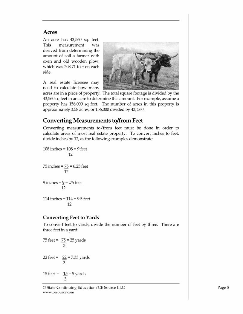
Acres An acre has 43,560 sq. feet. This measurement was derived from determining the amount of soil a farmer with oxen and old wooden plow, which was 208.71 feet on each side.
A real estate licensee may need to calculate how many acres are in a piece of property. The total square footage is divided by the 43,560 sq feet in an acre to determine this amount. For example, assume a property has 156,000 sq feet. The number of acres in this property is approximately 3.58 acres, or 156,000 divided by 43, 560.
Converting Measurements to/from Feet Converting measurements to/from feet must be done in order to calculate areas of most real estate property. To convert inches to feet, divide inches by 12, as the following examples demonstrate:
108 inches = 108 = 9 feet 12
75 inches = 75 = 6.25 feet 12 9 inches = 9 = .75 feet 12 114 inches = 114 = 9.5 feet 12
Converting Feet to Yards
To convert feet to yards, divide the number of feet by three. There are three feet in a yard:
75 feet = 75 = 25 yards 3
22 feet = 22 = 7.33 yards 3 15 feet = 15 = 5 yards 3

© State Continuing Education/CE Source LLC Page 6 www.cesource.com
Converting Feet to Acres
The real estate licensee may need to convert the square feet of a parcel to acres. An acre is 43,560 square feet. For example, a parcel is 400’ x 400’ feet. To calculate the number of acres, first find the area, then divide by 43,560:
400’ x 400’ = 160,000 square feet
160,000 square feet ÷ 43,560 square feet = 3.67 acres
The market price for farmland in the area is $10,000 per acre. An owner is considering selling a small tract which measures 360’ x 420’. If the tract sells at the current market price, how much will the owner receive?
Area = 360’ x 420’ = 151,200 square feet
# of Acres = 151,200 square feet ÷ 43,560 square feet = 3.47 acres
Price = $10,000 X 3.47 = $34,700
Front Feet
Front feet are used to measure real estate that has its frontage on some valuable item such as a lake, a river, or a specific street. When a lot is described, the front feet are always given first. A site may be priced per front foot:
60 ‘
120’
120’
Mt. View Lake
This type of lakefront property
may be priced per front foot at $1500 per front
foot: 60’ x $1500 =
$90,000.
A lot in the same area of the same size but without
lake frontage may be priced at $7 a square foot: 120’ x 60’ = 7200
sq. feet 7200 x $7 =
$50,400

© State Continuing Education/CE Source LLC Page 7 www.cesource.com
Commerce Avenue
Price Per Front Foot
To determine the price per front foot, divide the sales price by the front feet:
Price per front feet = sales price front feet
Price Per Front Foot Example
Jack is considering buying a lakefront property. He learns that a property there just sold for a little over $1,000,0000, and had frontage on the lake totaling 236 feet. About how much did the property sell per front foot?
$1,000,0000 = about $4,237 per front foot
236
Area of Triangles Sometimes the area of a triangle must be calculated when determining property size. The property may have a triangular section, for example.
The formula for finding the area of a triangle is:
Area = ½ (Base x Height)
750’
250’
A property is for sale in a sought- after business or
commercial district. It is desirable because of its
access to a main thoroughfare and is being sold by front feet. The price for this
property is $700 per front feet:
750’ x $900 = $675,000.
A similar sized commercial lot
nearby without the prestigious access
sells for $3 per square foot :
= 750’ x 250’ = 187,500 sq. feet
187,500 sq. ft x $3
= $562,500

© State Continuing Education/CE Source LLC Page 8 www.cesource.com
½ (14’ x 20’) = 140 square feet
Triangular Area Example 1
Calculate the area of the following property:
This property is made up of a rectangle and a triangle. First calculate the area of the rectangle:
150’ x 110’ = 16,500 square feet
Then, calculate the area of the triangle:
½ (40’ x 110’) = 2200 square feet
Total area = 16,500 square feet + 2200 square feet = 18,700 square feet
14’ Base
20’ Height
110’
150’ 40’

© State Continuing Education/CE Source LLC Page 9 www.cesource.com
Triangular Area Example 2
Calculate the area of the following property:
First, calculate the rectangle’s area: 140’ x 100’ = 14,000 square feet
Then, calculate the area of the small triangle. The base is 20 ‘ (160’ less 140’) : the area = ½ (20’ x 100’) = 1000 square feet
Then, calculate the large triangle: ½ (120’ x 160’) = 9600 square feet
The total area is: 14,000 + 1,000 + 9,600 = 24,600 square feet
In order to be able to calculate area in this way, the angles of the rectangle or square must be 90º angles, and the height of the triangle must be the highest point from the base that is perpendicular to the base.
Cubic Measurements To determine the area of a cube, or volume, the formula is:
Area of a cube, or Volume = Length x Width x Height
1 cubic foot = 1,728 cubic inches
1 cubic yard = 27 cubic feet
140’
100’
180’
120’
120’
160’

© State Continuing Education/CE Source LLC Page 10 www.cesource.com
In some cases, the volume, or cubic measurement of a space, must be calculated. For example, the client may want to measure a storeroom or warehouse to determine how much shelving or inventory it will contain. Or, the buyer of a residence may want to put in a swim pool, and needs to determine the cubic measurements for planning its installation.
Cubic Measurement Example
The prospective tenant wants to know the volume of the storage area in the building. The length of the storage area is 50’, the width is 35’ and the height is 10’.
Volume = 50’ x 35’ x 10’ = 17,500 cubic feet
Metric Equivalents Outside of the United States, the metric system is used to measure real property. Following are a few important metric equivalents to U.S. units of measurement:
Lengths
One foot = 0.3048 meter
One yard = 0.9144 meter
One mile = 1.6093 kilometers or 1609 meters
Areas
One square foot = 0.0928 square meters
One square yard = 0.836 square meters
One acre = 4068.8 square meters
One square mile = 259 hectares or 2.59 square kilometers
One square meter = 10.76 square feet
One hectare = 2.47 acres or 10,000 square meters
Metric Equivalent Example
A buyer from Canada would like the real estate licensee to give the area of the property in square meters. The property is 5 acres. How many square meters is it?
1 acre = 4068.8 square meters
5 acres = 5 X 4068.8 square meters = 20,344 square meters

© State Continuing Education/CE Source LLC Page 11 www.cesource.com
Summary of Measurements Linear Measurement Formulas
One foot = 12 inches
One yard = 3 feet or 36 inches
One rod = 16 ½ feet, or 5 ½ yards
100 feet = 6.6 rods
One mile = 5,280 feet; 1760 yards; 320 rods; or 80 chains
Perimeter Formula
Total the measurement of the boundaries of a space
Area Formulas
Area = length x Width
Length = Area ÷ Width
Width = Area ÷ Length
Area is stated in square units.
Square Measurements
1 square foot = 144 square inches
1 square yard = 9 square feet
1 square rod = 30 ¼ square yards
1 acre = 43,560 square feet
Converting Measurements to/from Feet
To convert inches to feet, divide the total number of inches by 12
To convert feet to yards, divide the total number of feet by 3
Converting Feet to Acres
To convert feet to acres, divide the number of feet by 43,560
Front feet are the number of feet on a property that borders the street or desirable feature such as a view of lake.

© State Continuing Education/CE Source LLC Page 12 www.cesource.com
Front Feet Formulas
Sales Price = Amount per front feet X Number of front feet
Price Per Front Feet = Sales Price ÷ Front Feet
Area of a Triangle
Area = ½ (Base X Height)
Area of a Cube (Volume)
Volume = Length X Width X Height
Metric Equivalents
One foot = 0.3048 meter
One yard = 0.9144 meter
One mile = 1.6093 kilometers or 1609 meters
Metric Areas
One square foot = 0.0928 square meters
One square yard = 0.836 square meters
One acre = 4068.8 square meters
One square mile = 259 hectares or 2.59 square kilometers
One square meter = 10.76 square feet
One hectare = 2.47 acres or 10,000 square meters
Legal Descriptions Real estate math is sometimes needed to read and understand legal property descriptions. Some property descriptions require that the real estate licensee understand linear measurements, how to calculate area and be able to read surveying directions, in order to understand the description.

© State Continuing Education/CE Source LLC Page 13 www.cesource.com
Metes-and-Bounds and Monument Descriptions One way property is described is through a metes-and-bounds and monument description. This is the most accurate way to describe a property parcel or lot. The word “metes” means “measurements.” “Bounds” refers to directions. In this method, measurements are taken of the property boundaries using monuments on the property. “Monuments” are streams, trees, piles of stones, iron pipes, posts, etc.
The directions from monument to monument along the property’s boundaries are stated in compass directions:
The directions of a compass are described as north, south, east, west, northeast, northwest, southeast and southwest, along with degrees, minutes and seconds. The total degrees in a circle, as in a compass are 360. Each quadrant in a circle has 90º.
N
E
S
W
90 º

© State Continuing Education/CE Source LLC Page 14 www.cesource.com
Metes and Bounds Example 1
If a metes and bounds description states, “South 40º East 100 feet, this means, from that point in the description, face south, and to 40º toward the East for 100 feet:
Metes and Bounds Example 2
Here is an example of a modern metes-and-bounds description:
“Commencing 62 feet West from the Southeast corner of Lot 1, Block 70, Plat D, Salt Lake City Survey, North 70 feet; East 12.5 feet; North 13º West 20 feet to ditch, Northwesterly along said ditch; North 31º West 68.75 feet; West 2.75 rods; East 53.5 feet to the beginning.”
The first direction in this description requires having a lots and blocks map of Salt Lake City, finding Lot 1, Block 70, in Plat D, and going West 62 feet from its Southeast corner.
The next direction, “North 70 feet” indicates the property line then goes due North for 70 feet. The direction “East 12.5 feet” indicates the property line then goes directly East 12.5 feet.
S
40º
100 ft

© State Continuing Education/CE Source LLC Page 15 www.cesource.com
Then, the description states “North 13º West 20 feet to ditch.” This means that from the last point, facing North, go 13º West, for 20 feet to the ditch:
Then, the description states “Northwesterly along said ditch,” which means that the ditch follows a northwesterly direction, and the property line follows this ditch. The next direction is “North 31º West 68.75 feet,” so the property line proceeds from the end of this ditch, facing north, going 31º West for 68.75 feet.
13º N
20 ft
W
N 31º
68.75 ft
© State Continuing Education/CE Source LLC Page 16 www.cesource.com
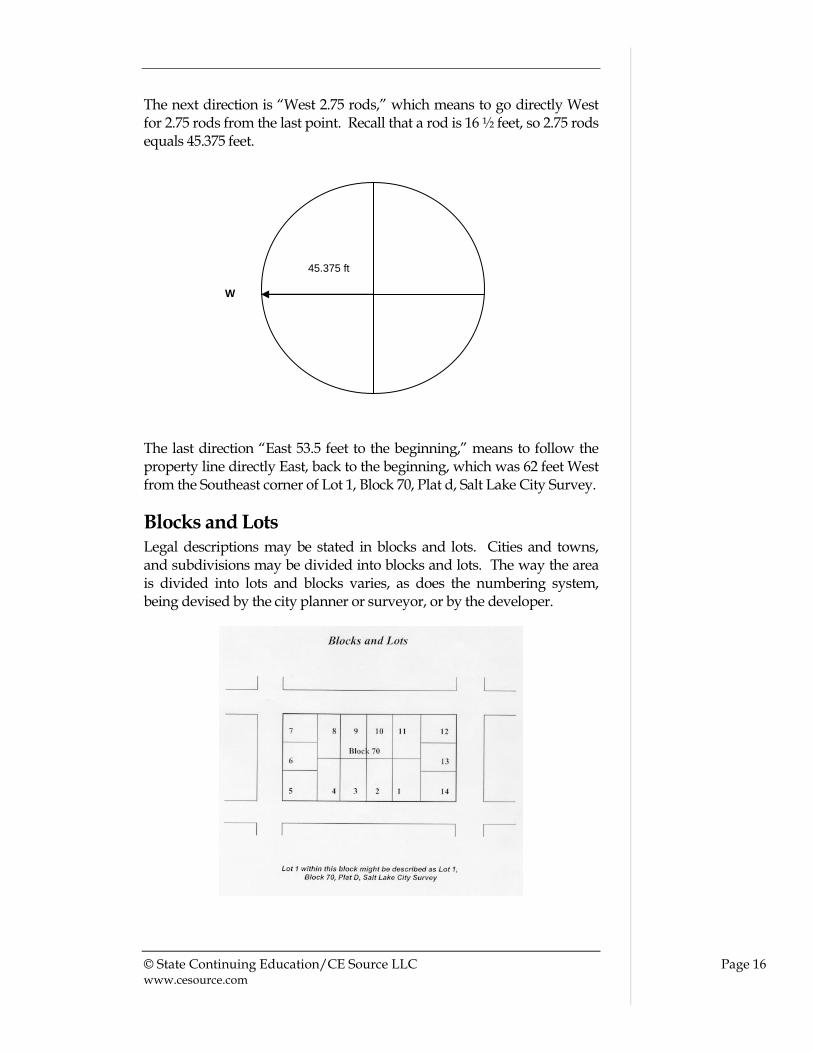
The next direction is “West 2.75 rods,” which means to go directly West for 2.75 rods from the last point. Recall that a rod is 16 ½ feet, so 2.75 rods equals 45.375 feet.
The last direction “East 53.5 feet to the beginning,” means to follow the property line directly East, back to the beginning, which was 62 feet West from the Southeast corner of Lot 1, Block 70, Plat d, Salt Lake City Survey.
Blocks and Lots Legal descriptions may be stated in blocks and lots. Cities and towns, and subdivisions may be divided into blocks and lots. The way the area is divided into lots and blocks varies, as does the numbering system, being devised by the city planner or surveyor, or by the developer.
W
45.375 ft

© State Continuing Education/CE Source LLC Page 17 www.cesource.com
Plats A plat is a map recorded by the County Clerk or Recorder that is drawn to show the legal boundaries of a property and its features, such as roads, creeks and alleys. A plat map may be of a whole town, an individual property, or of an area or subdivision.
U.S. Government Survey System Property descriptions may be based on the U.S. Government Survey System, also known as the Public Land Survey System (PLSS). This system was used in a large part of the United States, although not in Texas, when the U.S. Government distributed land gained through the Louisiana Purchase, the agreement to gain the Northwest Territory, and to purchase Alaska.
From http://nationalatlas.gov/articles/boundaries/a_plss.html
The territory in this system was divided by 35 meridians, each 24 miles apart, and by 32 baselines. Within the meridians and baselines, the area is divided into “checks,” which are 24 miles by 24 miles. Each check is divided into 16 “townships”, which are about 6 miles square, and are divided into 36 one-mile square “sections”.
© State Continuing Education/CE Source LLC Page 18 www.cesource.com
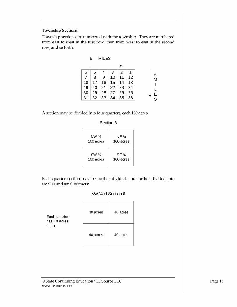
Township Sections
Township sections are numbered with the township. They are numbered from east to west in the first row, then from west to east in the second row, and so forth.
6 5 4 3 2 1
7 8 9 10 11 12
18 17 16 15 14 13
19 20 21 22 23 24
30 29 28 27 26 25
31 32 33 34 35 36
A section may be divided into four quarters, each 160 acres:
Section 6
NW ¼
160 acres
NE ¼
160 acres
SW ¼
160 acres
SE ¼
160 acres
Each quarter section may be further divided, and further divided into smaller and smaller tracts:
NW ¼ of Section 6
40 acres
40 acres
40 acres
40 acres
6 M I L E S
6 MILES
Each quarter has 40 acres each.

© State Continuing Education/CE Source LLC Page 19 www.cesource.com
NE ¼ of NW ¼ of Section 6
10 acres
10 acres
10 acres
10 acres
NW ¼, NE ¼ of NW ¼ of Section 6
2.5 acres
2.5 acres
2.5 acres
2.5 acres
Each quarter section can be divided into quarters of 10 acres each.
They can be further divided into quarters of 2.5 acres each.

© State Continuing Education/CE Source LLC Page 20 www.cesource.com
Calculating Number of Acres in a Tract
To calculate the number of acres in a tract in a government survey description, remember that a section has 640 acres. If a tract has the NW ¼, SE ¼, NE ¼ of Section 12, this means the tract shaded in the following diagram:
Section 12
NW ¼
NW ¼ 40 acres
NE 1/4
SW ¼
10 acres
NW ¼
SE ¼
SW ¼
SW ¼
SE ¼
To calculate the acres mathematically, the formula is:
640 acres ÷ 4 ÷ 4 ÷ 4 = 10 acres in this tract (Section 12) (NE ¼ ) (SE ¼ ) (NW ¼ )
How many acres are in tract SW ¼ of the NW ¼ of Section 20?
Section 20
NW ¼
NE ¼
NE ¼
SW ¼
SE ¼
SW ¼
SE ¼

© State Continuing Education/CE Source LLC Page 21 www.cesource.com
640 acres ÷ 4 ÷ 4 = 40 acres
How many acres total are in these two tracts: NW ¼, SW ¼ of Section 26 and NE ¼, SE ¼ of Section 25?
Section 25 Section 26
NW ¼
NE ¼
NW ¼
NE ¼
SW ¼
NW ¼
NE ¼
NW ¼
NE ¼
SE ¼
SW ¼
SE ¼
SW ¼
SE ¼
640 acres ÷ 4 ÷ 4 = 40 acres + 640 acres ÷ 4 ÷ 4 = 40 acres = 80 acres
Summary of Legal Descriptions Metes-and-Bounds Legal Descriptions - Measurements are taken of the property boundaries using monuments on the property. Directions from point to point are defined using compass directions.
Lots and Blocks Legal Descriptions – Cities, towns, subdivisions are divided into lots and blocks, which are numbered, and referred to in legal descriptions.
Plats – A map recorded by the County Clerk or Recorder drawn to show the legal boundaries of a property and its features, such as roads, creeks and alleys.
U.S. Government Survey System – Land distributed by the Federal government which was divided by 35 meridians, 24 miles apart, and by 32 baselines.
Division measurements in the U.S. Government Survey System
Checks = 24 x 24 miles
Townships = 6 miles square
Sections = 1 mile square

© State Continuing Education/CE Source LLC Page 22 www.cesource.com
Quarter Sections = 160 acres
Quarter sections are further divided by quarters, and so forth to smaller and smaller areas:
160 acres ÷ 4 = 40 acres
40 acres ÷ 4 = 10 acres
10 acres ÷ 4 = 2.5 acres
Each quarter is identified by its location in a Section: NW ¼, NE ¼, SW ¼ or SE ¼

© State Continuing Education/CE Source LLC Page 23 www.cesource.com
CHAPTER TWO
PPEERRCCEENNTTAAGGEESS,, IINNTTEERREESSTT AANNDD
MMOORRTTGGAAGGEESS
Calculating interest is a mathematical concept used by a real estate licensee in many situations. Percentages are used in calculating interest and other real estate related equations. Mortgage calculations rely upon a knowledge of interest computations. This chapter explains real estate calculations using percentages and interest. Upon completion of this chapter, you will be able to:
Convert a percentage to a decimal
Use percentages to calculate earnest money, depreciation, and other amounts
Use percentages to calculate commissions
Use percentages to calculate return on investment
Perform simple interest rate calculations to find the rate, time and principal
Calculate annual, quarterly, monthly and daily interest rates
Prorate daily interest
Perform compound interest calculations
Calculate a down payment
Calculate the loan to value ratio
Calculate a mortgage insurance premium
Calculate a loan commitment fee
Calculate a loan origination fee
Calculate loan payment to income ratios
Calculate debt to income ratios
Calculate the principal in a loan payment
Notes

C H A P T E R 2 : I N T E R E S T A N D M O R T G A G E S
© State Continuing Education/CE Source LLC Page 24 www.cesource.com
Calculate loan principal and interest
Calculate a total loan payment of principal, interest, taxes and insurance
Calculate an amortized loan payment using a table
Percentages Interest rates use percentages. Percentage means “parts of a 100.” To find a percentage of a number, the number is multiplied by the percentage. The percentage should be written as a decimal: 5% = 0.5, 10% = 0.10, 25% = 0.25, 50% = 0.50, 75% = 0.75, 100% = 1.00, etc. Then, the decimal form of the percentage may be multiplied, divided, or otherwise used in equations.
For example, 25% x 140 is rewritten as .25 x 140. The calculation can be written in columnar form:
140 x .25
35.00, or 35
Calculating Percentage Problems
In calculating problems involving percentages, three components are used: the Rate, the Total and the Part. The percentage rate multiplied by a number gives a part of the number.
For example, a prospective buyer wants to offer 2% of the offer price as earnest money. The offer price is $200,000. As a percentage problem, $200,000 is the Total, 2% is the Rate, and the earnest money amount is the Part. To calculate the earnest money amount, the situation is converted to a multiplication problem: 2% of $200,000 = the earnest money. The “of” in this problem is changed to “times” in the multiplication problem:
2% x $200,000 = $4,000 (Rate x Total = Part)
or, it is also correct to state it as:
$200,000 x 2% = $4,000 (Total x Rate = Part)
This formula can be used to find the total when the rate and part are known, as well:
Total = Part Rate

C H A P T E R 2 : I N T E R E S T A N D M O R T G A G E S
© State Continuing Education/CE Source LLC Page 25 www.cesource.com
For example, the client made a 15% down payment on a home. The down payment amount was $26,700. How much was the purchase price of the home?
$26,700 = $178,000 .15
Percentage of Depreciation
Another percentage problem that may need to be solved by a real estate licensee occurs when a buyer purchases some personal property from the seller, and wants to pay depreciated value. For example, the personal property is the seller’s home theater equipment and furniture in the home theater room. The buyer and seller settle on 50% of the purchase price as the amount. The total is $7,000, the rate is 50%, and the “part” is the resulting amount the buyer will pay:
$7,000 x 50% = $3,500 (Total X Rate = Part)
Percentage of Purchase Price
Or, a buyer may want to evaluate an asking price a seller gives for buying some personal property by determining the percentage of the purchase price the seller is asking for the property. The personal property is one-year old furniture, that the seller is asking $3,000. The buyer asks what the seller paid and is told $5,000. This can be restated as this question, “What % of $5,000 is $3,000?” The formula used is:
Rate = Part , or Rate = $3,000 which equals 60%. Total $5,000
The buyer can decide whether he believes 60% of the original price is fair to pay for this personal property.
Converting a Percentage to a Decimal
A percentage is converted to a decimal by dropping the percentage sign and moving the decimal point two places to the left:
10% = .10
100% = 1
95% = .95
25% = 25
46% = .46
C H A P T E R 2 : I N T E R E S T A N D M O R T G A G E S
© State Continuing Education/CE Source LLC Page 26 www.cesource.com
4% = .04
3.5% = 0.35
1.25% = .0125
Converting a Decimal to a Percentage
A decimal is converted to a percentage by moving the decimal point two places to the right, and adding a percent sign:
.125 = 12.5%
1.00 = 100%
2.65 = 265%
.0025 = .25%
.01 = 1%
.04 = 4%
.0625 = 6.25%
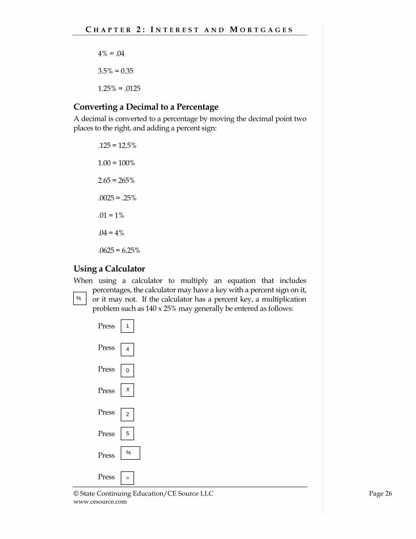
Using a Calculator
When using a calculator to multiply an equation that includes percentages, the calculator may have a key with a percent sign on it, or it may not. If the calculator has a percent key, a multiplication problem such as 140 x 25% may generally be entered as follows:
Press
Press
Press
Press
Press
Press
Press
Press
%
1
4
0
X
2
5
%
=

C H A P T E R 2 : I N T E R E S T A N D M O R T G A G E S
© State Continuing Education/CE Source LLC Page 27 www.cesource.com
Answer: 35
If the calculator does not have a percent key, the percentage needs to be entered as a decimal:
Press
Press
Press
Press
Press
Press
Press
Press
Answer: 35
Commission
Another type of problem where percentages are used is when commission is involved. A seller may want to know what the seller will receive, net of commission, if a buyer pays the asking price. The broker’s commission is 6%, and the asking price is $200,000. The rate for this problem is not 6%, however. It is 94%, or 100% less the 6% commission, because this is the rate of the total the seller will receive. The formula for this problem is:
Seller’s Net Proceeds = Rate x Total, or 94% x $200,000 = $188,000.
The broker calculates his or her commission with this formula:
Part (the commission) = Rate x Whole (Selling Price)
The commission rate is 6%, and the selling price is $250,000:
Commission = 6% x $250,000
Commission = $15,000
1
4
0
X
.
.
. 2
5
=

C H A P T E R 2 : I N T E R E S T A N D M O R T G A G E S
© State Continuing Education/CE Source LLC Page 28 www.cesource.com
Splitting Commissions
When commission is being calculated, the problem may have to be broken into steps. For example, the calculation is more complicated when the commission is being split: The listing agent negotiates a 6% commission rate with the seller, and agrees to split the commission with another agent in the brokerage. The listing agent will get 60% of the commission, and the other agent 40%. The selling price is $350,000.
First, find the total commission using the equation:
Part = Rate x Whole, or
Commission = Rate x Selling Price, or 6% x $350,000 = $21,000
Second, find the listing agent’s commission = 60% x $21,000 = $12,600
Third, find the other agent’s commission = $21,000 - $12,600 = $8,400 or
40% x $21,000 = $8,400
Let’s look at another example of this type of commission calculation. A home sells for $175,300. The listing broker will receive ¾ of the commission, and the salesperson will receive ¼ of the commission. The total commission for the sale was 6%.
First, calculate the total commission:
Commission = Rate x Selling Price
Commission = 6% x $175,300 = $10,518
Then, convert the fractional split to percentages:
Broker’s commission = ¾ = 75%
Salesperson’s commission = ¼ = 25%
Third, calculate the broker’s commission:
Broker’s commission = 75% x $10,518 = $7888.50
Finally, calculate the salesperson’s commission:
Salesperson’s commission = 25% x $10,518 = $2,629.50, or
$10,518 - $7888.50 = $2,629.50

C H A P T E R 2 : I N T E R E S T A N D M O R T G A G E S
© State Continuing Education/CE Source LLC Page 29 www.cesource.com
Verifying Commissions
Possibly, a broker or salesperson may want to verify commissions he or she was paid were calculated properly. If the broker or salesperson knows the commission amount received and the rate, he or she can calculate the sales price, and verify the result with the actual sales price of the property. For this problem, the formula:
Whole = Part (Commission) Rate (Commission Rate) is used.
The broker received a commission check for $19,500. The commission rate for the sale was 6%. What is the sales price? Sales Price = $19,500 = $325,000 6%
Calculating Incremental Commissions
Another scenario involving commissions is when the commission rate changes based on the amount of production, or the amount of the sale. For example, a broker may pay a salesperson 50% of the broker’s commission for sales production up to $300,000, 55% of the commission for production above $300,000 to $600,000 and 60% of the commission for production above $600,000.
Or, a broker may negotiate with a client that he or she be paid a commission of 6% on the first $250,000 of the sales price, 7% on the next $500,000, 8% on the next $500,000 and 10% on the amount over $1,250,000. To calculate these types of problems, each portion of the commission or sale with a different rate is computed separately and then totaled.
Incremental Commission Example 1
The broker negotiated with the owner of an office complex to list the office complex with the following commission schedule:
5% on first $500,000
7% on the next $500,000
8% on the next $500,000
10% on any amount over $1,500,000
The building sells for $1,950,000. The commission is calculated as follows:
1. $500,000 x 5% = $25,000
2. $500,000 x 7% = $35,000
3. $500,000 x 8% = $40,000

C H A P T E R 2 : I N T E R E S T A N D M O R T G A G E S
© State Continuing Education/CE Source LLC Page 30 www.cesource.com
4. $450,000 x 10% = $45,000
5. $25,000 + $35,000 + $40,000 + $45,000 = $145,000 total commission
Incremental Commission Example 2
The salesperson has a commission schedule as follows:
50% of the commission for sales production up through $300,000
55% of the commission for sales production over $300,000 through $500,000
60% of the commission for sales production over $500,000 through $750,000
The first home the salesperson sells is sold for $250,000, and the broker’s commission was 7%. What is the salesperson’s commission?
Broker’s commission = $250,000 x 7% = $17,500
Salesperson’s commission = $17,500 x 50% = $8,750
The salesperson then sells a home for $275,000. The broker’s commission is 6%. What is the salesperson’s commission for this sale?
The salesperson is going to move to the next commission level once the salesperson’s production is over $300,000. Since the salesperson has previously sold $250,000, $50,000 of this sale will be at the 50% of the commission amount, and the next $225,000 will be at the next level, which is 55% of the commission amount. The broker’s commission can be calculated based on these two figures, and then the salesperson’s commission calculated at the two different percentages:
$50,000 x 6%= $3000 (broker’s commission) x 50% = $1500
$225,000 x 6% = $13,500 (broker’s commission) x 55% = $7425
$1500 +$7425 = $8925 salesperson commission
Rate of Return
Percentages are also used when dealing with investment and business property. For example, a prospective investor finds out the current investors are receiving $10,000 annually from a real estate investment that

C H A P T E R 2 : I N T E R E S T A N D M O R T G A G E S
© State Continuing Education/CE Source LLC Page 31 www.cesource.com
has investment costs of $125,000. The prospective investor wants to determine the percentage return the current investors are receiving. For this type of problem, the formula: Rate of Return = Income Investment Rate = $10,000 = 8%. $125,000 The current investors are making 8% return on their investment.
This type of percentage problem will be discussed again when the course deals with investments.
Calculating Interest There are two basic interest calculations with which the real estate agent and broker should be familiar. One is the formula for simple interest, and the other for compound interest. Simple interest is the rate applied to the principal only. Compound interest accrues interest on the principal plus the interest already earned.
Time
When dealing with interest calculations, a time element must be taken into consideration. This is why interest rate calculations are not identical to percentage calculations, even though there is a percentage rate involved.
Normally Annual
Interest is usually quoted as an annual figure. A bank certificate of deposit that advertises a 4% yield is giving an annualized interest rate, for example. After one year, the amount in the certificate of deposit will have increased by 4%. If a car loan charges a 3% rate, this is also an annualized interest figure. Sometimes, rates are quoted for periods longer than a year. For example, a mutual fund may boast a 102% return since the date of its inception, or for a five or ten year period. Knowing the period of time that is used when a rate is quoted is very important.
Compounding Frequencies
Part of the time element issue in interest rates is the way the annualized rate is calculated during the year. The interest may be compounded during the period. When interest compounds, the interest earned is added to the original sum, and the interest earned is then based on this new amount. Interest may compound daily, weekly, monthly, semi-annually, or at some other frequency. The most common compounding frequencies are daily, monthly, and annually.

C H A P T E R 2 : I N T E R E S T A N D M O R T G A G E S
© State Continuing Education/CE Source LLC Page 32 www.cesource.com
Defining a Year
Another time element related issue in interest rate calculations is the number of days used to determine the annual rate. Interest may be calculated using a 365-day year, or a 360-day year. This is another component of an interest rate that needs to be taken into account in order to understand the true value of the rate quoted. For example, if a daily rate is .045, the annualized rate for a 365-day year would be 16.425%, and for a 360-day year would be 16.20%. The use of the 360-day year stems from before the days of calculators and computers; 360 is an easier number to use in mathematical calculations than is 365.
If interest does not compound other than annually, the interest rate is said to be a “simple” interest rate. The term “simple” is used when the rate is quoted on an annual basis.
Simple Interest Formula The simple Interest (I) formula is Principal (P) x Rate (R) x Time (T), or I = PRT.
For example, the simple interest on $10,000 for 5 years at 10% is:
$10,000 x 5 x .10 = $5000
Each of the variables in the simple interest calculation can be found by rearranging the equation:
Finding the Rate
What is the Rate of interest if $5000 earns $300 in 2 years?
R = I÷ PT
R = $300 ÷ ($5000 x 2)
R = .03 or 3%
Finding the Time
How long will it take to earn $750 on $10,000 earning 5% annually?
T = I ÷ PR
T = $750 ÷ ($10,000 x .05)
T= 1.5 years

C H A P T E R 2 : I N T E R E S T A N D M O R T G A G E S
© State Continuing Education/CE Source LLC Page 33 www.cesource.com
Finding the Principal
How much must be loaned to receive interest of $2000 after 5 years at 8%?
P = I ÷ TR
P=$2000 ÷ (5 x .08)
P = $5000
Finding Annual Interest
When the amount of annual interest is being found, the formula is the same as the simple interest calculation:
Annual interest = principal x rate
Quarterly Interest
To calculate quarterly interest from a simple annual rate, the formula is:
Quarterly interest = annual interest ÷ 4
For example, a buyer is required to pay quarterly interest on a $20,000 loan for one year. If the interest on the loan is 9%, what is the quarterly interest payment?
I = PRT
I = $20,000 x (9% ÷ 4) = $450
Monthly Interest
To calculate monthly interest from a simple annual rate, the formula is:
Monthly interest = annual interest ÷ 12
Daily Interest
To calculate daily interest from a simple annual rate, the formula rate is:
Daily interest = annual interest ÷ 365 or annual interest ÷ 360
Prorating and Daily Interest
Daily interest is sometimes used to calculate prorating parts of a month. In this case, the monthly interest is divided by the number of days in the month, and then multiplied by the number of days being prorated:
Monthly interest ÷ # of days in month = daily interest

C H A P T E R 2 : I N T E R E S T A N D M O R T G A G E S
© State Continuing Education/CE Source LLC Page 34 www.cesource.com
Or, the formula used for prorating may be to start with the annual interest, dividing it by number of days in the year (typically 360), then multiplying the daily interest by the number of days in the period to be prorated.
Daily Proration Example 1
For example, a seller’s mortgage is being assumed by a buyer. The buyer will assume the mortgage on the 20th of March. So, the seller will pay the mortgage through March 19th, and the buyer will begin paying the mortgage the 20th of March. The mortgage balance is $83,000 and the rate is 5%.
Annual interest = $83,000 x 5% = $4150
Daily interest = $4150 ÷ 360 = $11.53
For the seller, the mortgage interest for March = daily interest x 19 days = $11.53 x 19 = $219.07
For the buyer, the mortgage interest for March = daily interest x 12 days = $11.53 x 12 = $138.36
Daily Proration Example 2
If calculated for prorating the alternate way, by determining monthly interest and dividing by the number of days in the month, the result would be:
Monthly interest = annual interest ÷ 12
Monthly interest = $4150 ÷ 12 = $345.83
Daily interest for March = monthly interest ÷ 31 = $345.83 ÷ 31 = $11.16
For the seller = $11.16 x 19 days = $212.04
For the buyer = $11.16 x 12 days = $133.92
The person responsible for calculating this proration typically uses the first calculation, using the annual rate to determine the daily rate, because its more accurate. The mortgage company may provide these figures, but, if the mortgage was originally a seller-financed mortgage or was otherwise issued by an individual, a manual proration like this might be done. The mortgage note or loan itself needs to be looked at to determine the best method for calculating the interest proration, taking into consideration how the interest rate is stated, compounded, and applied to the mortgage or loan balance.

C H A P T E R 2 : I N T E R E S T A N D M O R T G A G E S
© State Continuing Education/CE Source LLC Page 35 www.cesource.com
Total Amount of Interest Earned
Jack is saving for a down payment on a home. If he puts $2,000 in an investment product that returned 7.5% over one year, how much interest will he earn? How much in total will he have at the end of a year?
I = PRT
I = $2000 x 7.5% x 1 = $150
Total at the end of the year = $2000 (original principal) + $150 (total interest earned) = $2,150
If Jack can add $100 to his $2000 at the beginning of each month, how much will he earn, assuming the same 7.5% simple interest earned throughout the whole year? In this situation, each month, the principal is increased by $100, and the monthly interest rate is applied to that amount. (These calculations are rounded to two decimal places.)
January = $2100 x (7.5% ÷ 12) = $13.13
February = $2200 x (7.5% ÷ 12) = $13.75
March = $2300 x (7.5% ÷ 12) = $14.38
April = $2400 x (7.5% ÷ 12) = $15.00
May = $2500 x (7.5% ÷ 12) = $15.63
June = $2600 x (7.5% ÷ 12) = $16.25
July = $2700 x (7.5% ÷ 12) = $16.88
August = $2800 x (7.5% ÷ 12) = $17.50
September = $2900 x (7.5% ÷ 12) = $18.13
October = $3000 x (7.5% ÷ 12) = $18.75
November = $3100 x (7.5% ÷ 12) = $19.38
December = $3200 x (7.5% ÷ 12) = $20.00
Total Interest = $ 198.78
At the end of the year, Jack will have about $3398.78 toward his down payment.

C H A P T E R 2 : I N T E R E S T A N D M O R T G A G E S
© State Continuing Education/CE Source LLC Page 36 www.cesource.com
Compound Interest Formula
The compound interest formulas are a little more complex than the simple interest formulas. Each compounding period, e.g., monthly, quarterly, semi-annual, annual, must be accounted for in a compound interest equation. The
compounding period is known as the “conversion period” for calculation purposes. The interest rate is usually stated as an annual rate and must be changed to a periodic interest rate (i) when compound interest is calculated. “i” is the annual interest rate divided by the conversion periods per year. The formula for compound interest is:
I = P x i
Compound Interest Example
How much interest is paid on a $15,000 loan charged 6% compounded quarterly for 1 year?
First quarter:
I = $15,000 x (.06÷4)
I = $15,000 x .015
I = $225 (1st quarter interest)
Second quarter:
I = $15,225 x .015
I = $228.38 (2nd quarter interest)
Third quarter:
I = $15,453.38 x .015
I = $231.08 (3rd quarter interest)
Fourth quarter:
I = $15,685.18 x .015
I = $235.28 (4th quarter interest)

C H A P T E R 2 : I N T E R E S T A N D M O R T G A G E S
© State Continuing Education/CE Source LLC Page 37 www.cesource.com
End of year = $15,920.46
Total interest for the year = $920.46
As can be seen, calculating compound interest in this way is very time consuming. There are compound interest tables that can be used, as well as financial calculators and software to make compound interest calculations easier. The formula used in these tables and calculators is:
S = P (1+i)n
S = the sum, or principal + compound interest
P = the original principal amount (or the present value of the sum)
i = the interest rate divided by the conversion periods per year
n = the number of conversion periods in the term
Compound Interest Tables
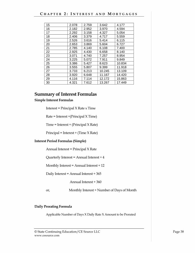
Compound interest tables can be used to determine how much interest will be paid or earned in many situations. They are available with various compounding periods and all interest rates. Following is a sample compound interest table with an annual compounding rate that shows compound interest rate factors for various years at various rates. When multiplied to the principal amount, the result is the sum of the principal + the compound interest after the number of years in the term.
For example, the total amount outstanding for a loan of $200,000 at 7% for 5 years is found by multiplying $200,000 by the factor found in the 7% column, 5-year row of the table, or 1.402. $200,000 x 1.402 = $280,400.
Sample Compound Interest Table (Annual Compounding)
Term (Years) 5% 7% 9% 10%
1 1.050 1.070 1.090 1.100
2 1.102 1.144 1.188 1.210
3 1.157 1.225 1.295 1.331
4 1.215 1.310 1.411 1.464
5 1.276 1.402 1.538 1.610
6 1.340 1.500 1.677 1.771
7 1.407 1.605 1.828 1.948
8 1.477 1.718 1.992 2.143
9 1.551 1.838 2.171 2.357
10 1.628 1.967 2.367 2.593
11 1.710 2.104 2.580 2.853
12 1.795 2.252 2.812 3.138
13 1.885 2.409 3.065 3.452
14 1.979 2.578 3.341 3.797
C H A P T E R 2 : I N T E R E S T A N D M O R T G A G E S
© State Continuing Education/CE Source LLC Page 38 www.cesource.com
15 2.078 2.759 3.642 4.177
16 2.182 2.952 3.970 4.594
17 2.292 3.158 4.327 5.054
18 2.406 3.379 4.717 5.559
19 2.526 3.616 5.414 6.115
20 2.653 3.869 5.604 6.727
21 2.785 4.140 6.108 7.400
22 2.925 4.430 6.658 8.140
23 3.071 4.740 7.257 8.954
24 3.225 5.072 7.911 9.849
25 3.386 5.427 8.623 10.834
26 3.555 5.807 9.399 11.918
27 3.733 6.213 10.245 13.109
28 3.920 6.648 11.167 14.420
29 4.116 7.114 12.172 15.863
30 4.321 7.612 13.267 17.449
Summary of Interest Formulas Simple Interest Formulas
Interest = Principal X Rate x Time
Rate = Interest ÷(Principal X Time)
Time = Interest ÷ (Principal X Rate)
Principal = Interest ÷ (Time X Rate)
Interest Period Formulas (Simple)
Annual Interest = Principal X Rate
Quarterly Interest = Annual Interest ÷ 4
Monthly Interest = Annual Interest ÷ 12
Daily Interest = Annual Interest ÷ 365
Annual Interest ÷ 360
or, Monthly Interest ÷ Number of Days of Month
Daily Prorating Formula
Applicable Number of Days X Daily Rate X Amount to be Prorated

C H A P T E R 2 : I N T E R E S T A N D M O R T G A G E S
© State Continuing Education/CE Source LLC Page 39 www.cesource.com
Total Amount Earned at End of Period Formula
1. Interest = Principal X Rate X Time
2. Total Earned = Principal + Interest
Compound Interest Formulas
Interest = P x I
i = annual interest divided by the conversion periods per year
Sum = Principal (1 + i)n
Mortgages and Math There are several financial components involved in a mortgage, including interest. These are:
Down payment
Loan amount
Discount points
Total loan payments, including principal, interest, taxes and insurance
Down Payments Today, there are a wide variety of mortgage products offered by lenders and other financial entities. Some products advertise no down payment, and others require 20% down payments, and many require amounts in between.
Calculating Down Payments
The formula used to calculate down payments is:
Selling Price x Down Payment Percent Required = Down Payment
Down Payment Example 1
The loan required a 5% down payment. The selling price of the home is $175,000. What is the required down payment?
Down payment = $175,000 (Selling Price) X 5% (Percent Required) = $8,750

C H A P T E R 2 : I N T E R E S T A N D M O R T G A G E S
© State Continuing Education/CE Source LLC Page 40 www.cesource.com
Down Payment Example 2
The bank requires a 20% down payment for its mortgage loan. The home is selling for $378,000. What is the amount of the required down payment?
Down payment = $378,000 X 20% = $75,600
Down Payment Example 3
The buyer has made a $7000 earnest money deposit. The home’s sales price is $215,000. The lender requires a 10% down payment. How much in addition to the earnest money does the buyer need for the down payment? This problem requires two steps – the first to calculate the total down payment, and the second to calculate the additional money needed:
Down payment = $215,000 X 10% = $21,500
Additional cash needed = $21,500 - $7,000 = $14,500
Calculating Loan – To –Value
One of the factors lenders use to determine whether they will underwrite a home loan is the amount of the loan as compared to the appraised value, or purchase price of the property. Some lenders will finance a maximum of 80% of the home’s value, some will finance close to 100%. The formula to determine the loan to value ratio is:
Loan Amount ÷ Property Value = Loan-to-Value Ratio
Loan-to-Value Example 1
The loan amount is $250,000. The value of the property is $290,000. What is the loan-to-value ratio?
$250,000 ÷ $290,000 = 86%
Loan-to-Value Example 2
The borrower wants to purchase a home worth $265,000. The lender will finance up to 90% of the home’s value. What is the maximum amount of the loan the lender will finance? The formula to calculate this amount is:
Property Value X Loan-to-Value Ratio = Maximum Loan Amount
$265,000 x .90 = $238,500
Loan-to-Value Example 3
What is the down payment needed if the lender will finance 80% of the purchase price for a home selling for $295,000?
Lender Financing = $295,000 X 80% = $236,000

C H A P T E R 2 : I N T E R E S T A N D M O R T G A G E S
© State Continuing Education/CE Source LLC Page 41 www.cesource.com
Down payment = $295,000 - $236,000 = $59,000
Loan-to-Value Example 4
The appraisal has been completed on the home, and it was appraised for less than $295,000. The appraised value is $283,000. The lender will finance 80% of the appraised value. What is the down payment needed?
Lender Financing = $283,000 X 80% = $226,400
Down payment = $283,000 - $226,400 = $56,600
FHA Loans Under the FHA 203(b) program, FHA will insure loans with relatively high amounts of lender financing. The maximum loan amount in most states is 98.75% of the sales price equal to or less than $50,000, and 97.75% of the sales price more than $50,000. The borrower must generally make a cash investment of 3% of the lesser of the purchase price or the appraised value in order for FHA to insure a loan with these percentages of lender financing.
FHA Financing Example
The borrower is buying a home selling at the appraised value of $90,000, and the borrower is able to make a 3% cash investment. What is the maximum loan amount FHA will insurer?
Maximum FHA insured loan amount = $90,000 X 97.75% = $87,975
How much is the cash investment the borrower must make on this home?
Borrower investment = $90,000 x 3% = $2700
Mortgage Insurance Premium Private Mortgage Insurance (PMI) covers the risk of the lender should the borrower default on a mortgage. Private mortgage insurance companies insure loans that meet their specific requirements. Generally, mortgages with loan-to-value ratios higher than 80% require PMI.
Lenders require PMI because if a lender has to foreclose, it wants to recoup the money it loaned. If a borrower puts down 20%, it is likely the lender will make back its money in a foreclosure situation. If a borrower does not have a 20% down payment, the lender wants to protect itself against the loss of the money it loaned.
The premiums for mortgage insurance are calculated using “points.” One point is the same as 1%, or .01. ½ point is .005. 1 ½ points is .015.

C H A P T E R 2 : I N T E R E S T A N D M O R T G A G E S
© State Continuing Education/CE Source LLC Page 42 www.cesource.com
The monthly premium for mortgage insurance is 1/12 of the annual premium.
Mortgage Insurance Premium Example
For example, assume the premium for mortgage insurance is .55 points, or .0055, and the loan amount is $115,000. The annual premium is $115,000 X .0055 = $632.50. The monthly premium is $632.50/12 = $52.71. This amount is added to the monthly loan principal and interest when calculating the total loan payment each month.
Loan Commitment Fees Another fee that may be charged along with a loan is a loan commitment fee. A loan commitment fee is required by a lender who promises to give a borrower constructing a home a loan once construction is complete. The loan commitment is required by the short-term lender financing construction in order to finance the short-term loan. The loan commitment fee is normally 1% of the promised long-term loan. Loan commitment fees may also be charged for other kinds of loans when a loan commitment is made.
What is the loan commitment fee for a $250,000 loan if the fee is 1%?
$250,000 x 1% = $2500
Loan Origination Fees The lender generally charges a fee for loan origination. This fee pays for the work done to process the loan. Generally, this fee is 1 point, or 1%.
How much is a 1% loan origination fee on a $195,000 loan?
$195,00 x 1% = $1950
Loan Discount Points A lender may charge discount points for giving a borrower a lower rate on the loan. For example, 1 point may be charged to reduce the loan rate from 5.75% to 5.25%.
Loan Discount Points Example 1
To get a 5.5% rate, the lender charges 1 point to the borrower of a $214,000 loan. How much does this loan discount cost the borrower?
$214,000 X 1% = $2140
C H A P T E R 2 : I N T E R E S T A N D M O R T G A G E S
© State Continuing Education/CE Source LLC Page 43 www.cesource.com
Loan Discount Points Example 2
To get a 5.0% rate, the lender charges 1.75 points on a $335,000 loan. How much does this loan discount cost the borrower?
$335,000 x 1.75% = $5,862.50
Qualifying For a Loan Lenders and government sponsored loan programs have different requirements that must be met in order for a borrower to qualify for a loan. Traditionally, for a conventional loan, where a 10% down payment is required, the total loan payment, meaning the principal, interest, tax and insurance, cannot exceed 28% of a borrower’s income. The amount of a borrower’s debt, including the loan payment, cannot exceed 36% of the borrower’s income.
Loan Payment to Income Ratio Example
For example, the borrower has monthly income of $4,000. The proposed loan payment is $1,100 per month. What is the loan payment to income ratio, expressed as a percentage? This is calculated by dividing the loan payment by the monthly income:
$1,100 ÷ $4,000 = .275, or 27.5%
Debt to Income Ratio Example
This same borrower has total monthly debt, including the loan payment is $2050. What is the debt to income ratio? This is calculated by dividing the total monthly debt by the monthly income:
$2050 ÷ $4,000 = .5125 or 51.25%
This borrower would not qualify for this loan, due to the high debt to income ratio.
FHA Requirements
To guarantee a loan, FHA allows a maximum housing to income ratio of 29%, and a total monthly debt to income ratio of 41%.
VA Requirements
The VA does not guarantee the entire loan amount. The general guarantee parameters are that the VA will guarantee ups to 25% of a home loan up to the Fannie Mae and Freddie Mac conforming loan limits, subject to the entitlement available to the veteran. Entitlement can be reduced if the veteran has obtained a VA loan in the past. Entitlement is restored if the
C H A P T E R 2 : I N T E R E S T A N D M O R T G A G E S
© State Continuing Education/CE Source LLC Page 44 www.cesource.com
mortgaged property has been sold and the loan has been paid in full, or if the loan has been assumed by another qualified veteran and that veteran agrees to substitute his or her entitlement for the same amount of entitlement the original borrower had used to get the loan. Entitlement can be restored one time only if a VA loan has been paid off, but the property has not been sold. The VA allows a monthly debt to income ratio of 41% for its loan program.
Real Estate Loans and Interest Often, an interest rate calculation is used by licensees when dealing with loans to purchase real estate. The interest rate is applied to the amount borrowed, which is called the “principal.” Interest adds, or “accrues” to the loan over time. Loan payments reduce the amount of principal and the accrued interest in the loan balance as they were made.
Loan Interest
For example, a home loan for $100,000 may be taken by a borrower. The loan has a 5.5% interest rate. If the rate is simple, and loan payments were not made to reduce the loan balance during the year, the amount of interest that would accrue on the loan would be $5500.
Loan Principal Calculation
To determine the principal amount on a loan, the formula used is: principal = interest
time x rate
If a loan has a 6% interest rate, the time period is one year, and the interest accrued was $636, the principal is calculated as follows:
principal = $636 = $10,600 1 x 6%
Principal and Interest Calculation
To determine the total amount, principal and interest, paid on a loan, the formula requires calculating the interest accrued, and adding it to the principal amount:
Step 1 Total Interest = PRT
Step 2 Interest + Principal = Total Amount Paid
If a loan is taken for $5000 with an 11% rate and is repaid at the end of one year, what is the total amount paid?
Total Interest = $5,000 x 11% x 1 = $550
Total Amount Paid = $5000 + $550 = $5,550

C H A P T E R 2 : I N T E R E S T A N D M O R T G A G E S
© State Continuing Education/CE Source LLC Page 45 www.cesource.com
If the loan was paid off in nine months, an additional step of calculating the interest for nine months rather than one year must be done:
Annual interest = $5,000 x 11% x 1 = $550
Nine months of interest = ($550 ÷ 12) x 9 = $412.50
Total amount paid = $5,000 + $412.50 = $5,412.50
Daily Interest Rate Tables
To streamline the interest calculation process, interest tables are used. A daily interest table based on a 360-day year usually gives interest rate figures from days 1 to 30. When interest is calculated for a period of days greater than 30, periods of up to 30 days are calculated separately and added together. For example, to determine the interest on $3,550 at 7% for 22 days using the following Daily Interest Rate Table for $1000, find the 7% daily rate column and the 22 day row, and use the daily factor .2778. Then, convert the $3,550 to $3.55 thousands:
$3.55 x 4.2778 = $15.19
To calculate the interest on $3,550 at 7% for 45 days, find the 7% daily rate corresponding to 30 days, and for 15 days:
30 days = $ 3.55 x 5.8333 = $20.71
15 days = $ 3.55 x 2.9167 = $10.35
45 days = $20.71 + $10.35 = $31.06
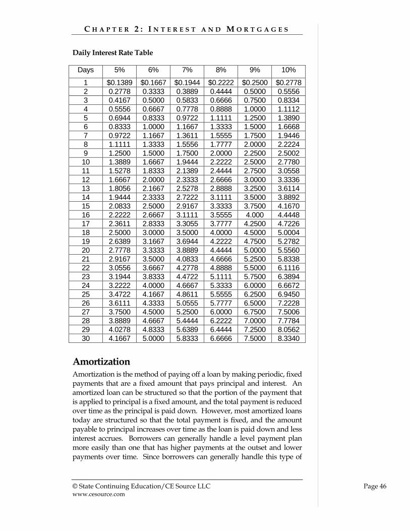
C H A P T E R 2 : I N T E R E S T A N D M O R T G A G E S
© State Continuing Education/CE Source LLC Page 46 www.cesource.com
Daily Interest Rate Table
Days 5% 6% 7% 8% 9% 10%
1 $0.1389 $0.1667 $0.1944 $0.2222 $0.2500 $0.2778
2 0.2778 0.3333 0.3889 0.4444 0.5000 0.5556
3 0.4167 0.5000 0.5833 0.6666 0.7500 0.8334
4 0.5556 0.6667 0.7778 0.8888 1.0000 1.1112
5 0.6944 0.8333 0.9722 1.1111 1.2500 1.3890
6 0.8333 1.0000 1.1667 1.3333 1.5000 1.6668
7 0.9722 1.1667 1.3611 1.5555 1.7500 1.9446
8 1.1111 1.3333 1.5556 1.7777 2.0000 2.2224
9 1.2500 1.5000 1.7500 2.0000 2.2500 2.5002
10 1.3889 1.6667 1.9444 2.2222 2.5000 2.7780
11 1.5278 1.8333 2.1389 2.4444 2.7500 3.0558
12 1.6667 2.0000 2.3333 2.6666 3.0000 3.3336
13 1.8056 2.1667 2.5278 2.8888 3.2500 3.6114
14 1.9444 2.3333 2.7222 3.1111 3.5000 3.8892
15 2.0833 2.5000 2.9167 3.3333 3.7500 4.1670
16 2.2222 2.6667 3.1111 3.5555 4.000 4.4448
17 2.3611 2.8333 3.3055 3.7777 4.2500 4.7226
18 2.5000 3.0000 3.5000 4.0000 4.5000 5.0004
19 2.6389 3.1667 3.6944 4.2222 4.7500 5.2782
20 2.7778 3.3333 3.8889 4.4444 5.0000 5.5560
21 2.9167 3.5000 4.0833 4.6666 5.2500 5.8338
22 3.0556 3.6667 4.2778 4.8888 5.5000 6.1116
23 3.1944 3.8333 4.4722 5.1111 5.7500 6.3894
24 3.2222 4.0000 4.6667 5.3333 6.0000 6.6672
25 3.4722 4.1667 4.8611 5.5555 6.2500 6.9450
26 3.6111 4.3333 5.0555 5.7777 6.5000 7.2228
27 3.7500 4.5000 5.2500 6.0000 6.7500 7.5006
28 3.8889 4.6667 5.4444 6.2222 7.0000 7.7784
29 4.0278 4.8333 5.6389 6.4444 7.2500 8.0562
30 4.1667 5.0000 5.8333 6.6666 7.5000 8.3340
Amortization Amortization is the method of paying off a loan by making periodic, fixed payments that are a fixed amount that pays principal and interest. An amortized loan can be structured so that the portion of the payment that is applied to principal is a fixed amount, and the total payment is reduced over time as the principal is paid down. However, most amortized loans today are structured so that the total payment is fixed, and the amount payable to principal increases over time as the loan is paid down and less interest accrues. Borrowers can generally handle a level payment plan more easily than one that has higher payments at the outset and lower payments over time. Since borrowers can generally handle this type of

C H A P T E R 2 : I N T E R E S T A N D M O R T G A G E S
© State Continuing Education/CE Source LLC Page 47 www.cesource.com
payment plan better than the alternative, this is the type of plan lenders generally offer.
Amortized Loan Illustrations
Amortization loan illustrations provide the outstanding loan balance, principal payment, interest payment and total interest paid for a loan amount, given a specified rate and term. Lenders provide sample amortization tables showing payments on a monthly or annual basis. In an amortized loan, the principal and interest are reduced as each payment is made.
Sample Amortization Loan Table – First Three Years
Loan Amount: $200,000, Rate: 7%, Loan Term: 30 Years, Monthly Payment: $1330.61
Month Loan Balance
Interest Principal Total Interest
1 199,836.06 1,166.67 163.94 1,166.67
2 199,671.17 1,165.71 164.90 2,332.38
3 199,505.31 1,164.75 165.86 3,497.13
4 199,338.49 1,163.78 166.83 4,660.91
5 199,170.69 1,162.81 167.80 5,823.72
6 199,001.91 1,161.83 168.78 6,985.55
7 198,832.15 1,160.84 169.77 8,146.39
8 198,661.40 1,159.85 170.76 9,306.24
9 198,489.66 1,158.86 171.75 10,465.10
10 198,316,91 1,157.86 172.75 11,622.96
11 198,143.15 1,156.85 173.76 12,779.81
12 197,968.38 1,155.84 174.77 13,935.65
13 197,792.59 1,154.82 175.79 15,090.47
14 197,615.78 1,153.80 176.81 16,244.27
15 197,437.93 1,152.76 177.85 17,397.03
16 197,259.05 1,151.72 178.89 18,548.75
17 197,079.12 1,150.68 179.93 19,699.43
18 196,898.14 1,149.63 180.98 20,849.06
19 196,716.11 1,148.57 182.04 21,997.63
20 196,533.02 1,147.51 183.09 23,145.14
21 196,348.85 1,146.44 184.17 24,291.58
22 196,163.62 1,145.37 185.24 25,436.95
23 195,977.30 1,144.29 186.32 26,581.24
24 195,789.89 1,143.20 187.41 27,724.44
25 195,601.40 1,142.11 188.50 28,866.55

C H A P T E R 2 : I N T E R E S T A N D M O R T G A G E S
© State Continuing Education/CE Source LLC Page 48 www.cesource.com
26 195,411.80 1,141.01 189.60 30,007.56
27 195,221.10 1,139.90 190.71 31,147.46
28 195,029.28 1,138.79 191.82 32,286.25
29 194,836.35 1,137.67 192.94 33,423.92
30 194,642.29 1,136.55 194.06 34,560.47
31 194,447.10 1,135.41 195.20 35,695.88
32 194,250.77 1,134.27 196.34 36,830.15
33 194,053.29 1,133.13 197.48 37,963.28
34 193,854.66 1,131.98 198.63 39,095.26
35 193,654.88 1,130.82 199.79 40,226.08
36 193,453.93 1,129.65 200.96 41,355.73
Amortization Loan Payment Tables
To determine monthly payments on a fixed payment, amortized loan, amortization payment tables can be used. Typically, these tables are stated in rates per $1000 of the loan.
Amortized Loan Payment Example 1
For example, to find the monthly payment on a $100,000 loan at 5.5% for 20 years, find the factor corresponding to the column 5.5% in the table on the following page, and the row 20 years, or 6.88. Multiply this factor by $100 ($100,000 loan divided by $1000 = $100).
6.88 x $100 = $688 monthly amortized loan payment
This figure reflects the principal and interest only in the loan, and does not include any taxes or insurance that are sometimes paid by borrowers with their home loan payments.
Amortized Loan Payment Example 2
As a further example, to find a monthly payment on a loan for $365,000 at 6.5% for 30 years, find the monthly payment factor for the 6.5% column in the table on the following page and the 30 year row = 6.33. Divide $365,000 by $1000 to get $365 to be multiplied by 6.33.
6.33 x $365 = $2310.45 monthly amortized loan payment
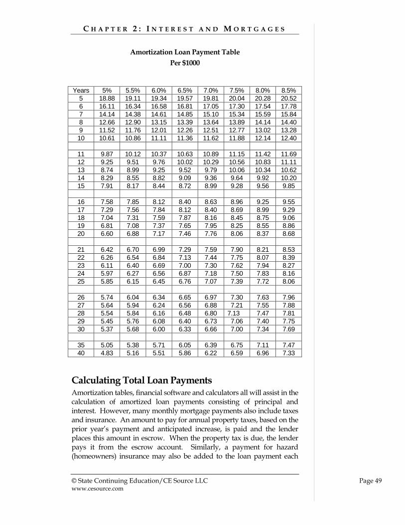
C H A P T E R 2 : I N T E R E S T A N D M O R T G A G E S
© State Continuing Education/CE Source LLC Page 49 www.cesource.com
Amortization Loan Payment Table
Per $1000
Years 5% 5.5% 6.0% 6.5% 7.0% 7.5% 8.0% 8.5%
5 18.88 19.11 19.34 19.57 19.81 20.04 20.28 20.52
6 16.11 16.34 16.58 16.81 17.05 17.30 17.54 17.78
7 14.14 14.38 14.61 14.85 15.10 15.34 15.59 15.84
8 12.66 12.90 13.15 13.39 13.64 13.89 14.14 14.40
9 11.52 11.76 12.01 12.26 12.51 12.77 13.02 13.28
10 10.61 10.86 11.11 11.36 11.62 11.88 12.14 12.40
11 9.87 10.12 10.37 10.63 10.89 11.15 11.42 11.69
12 9.25 9.51 9.76 10.02 10.29 10.56 10.83 11.11
13 8.74 8.99 9.25 9.52 9.79 10.06 10.34 10.62
14 8.29 8.55 8.82 9.09 9.36 9.64 9.92 10.20
15 7.91 8.17 8.44 8.72 8.99 9.28 9.56 9.85
16 7.58 7.85 8.12 8.40 8.63 8.96 9.25 9.55
17 7.29 7.56 7.84 8.12 8.40 8.69 8.99 9.29
18 7.04 7.31 7.59 7.87 8.16 8.45 8.75 9.06
19 6.81 7.08 7.37 7.65 7.95 8.25 8.55 8.86
20 6.60 6.88 7.17 7.46 7.76 8.06 8.37 8.68
21 6.42 6.70 6.99 7.29 7.59 7.90 8.21 8.53
22 6.26 6.54 6.84 7.13 7.44 7.75 8.07 8.39
23 6.11 6.40 6.69 7.00 7.30 7.62 7.94 8.27
24 5.97 6.27 6.56 6.87 7.18 7.50 7.83 8.16
25 5.85 6.15 6.45 6.76 7.07 7.39 7.72 8.06
26 5.74 6.04 6.34 6.65 6.97 7.30 7.63 7.96
27 5.64 5.94 6.24 6.56 6.88 7.21 7.55 7.88
28 5.54 5.84 6.16 6.48 6.80 7.13 7.47 7.81
29 5.45 5.76 6.08 6.40 6.73 7.06 7.40 7.75
30 5.37 5.68 6.00 6.33 6.66 7.00 7.34 7.69
35 5.05 5.38 5.71 6.05 6.39 6.75 7.11 7.47
40 4.83 5.16 5.51 5.86 6.22 6.59 6.96 7.33
Calculating Total Loan Payments Amortization tables, financial software and calculators all will assist in the calculation of amortized loan payments consisting of principal and interest. However, many monthly mortgage payments also include taxes and insurance. An amount to pay for annual property taxes, based on the prior year’s payment and anticipated increase, is paid and the lender places this amount in escrow. When the property tax is due, the lender pays it from the escrow account. Similarly, a payment for hazard (homeowners) insurance may also be added to the loan payment each
C H A P T E R 2 : I N T E R E S T A N D M O R T G A G E S
© State Continuing Education/CE Source LLC Page 50 www.cesource.com
month, and paid annually by the lender from the resulting accrued escrow amount.
The total payment is known as PITI, which stands for principal, interest, property taxes and insurance.
To determine the total loan payment, first use an amortization table, financial calculator or software to find the amount of the payment for principal and interest. Then, figure the monthly tax and insurance payment and add it to this amount to add the total principal, interest, tax and insurance payment.
PITI Calculation Example
For example, the amortized loan payment is $867 per month. The annual property taxes are $2432, and the annual homeowners payment is $832:
$2432 ÷ 12 = $202.67 (monthly tax payment)
$ 832 ÷ 12 = $69.33 (monthly insurance payment)
$202.67 + 69.33 = $272.00
PITI = $272 + 867 = $1139
Calculating Interest and Principal in Amortized Loans An amortized loan is one that regularly and systematically liquidates the debt. Each payment includes part principal and part interest. The factors needed to calculate how the amortized payments are divided between the principal and interest are the amount of the loan, or the principal, the rate of interest, and the amount of the payment per period.
Principal and Interest in Amortized Payment Example
For example, a client is given a quote of $852 per month for a loan with a 5.5% rate and an amount of $150,000. The client asks the licensee how much interest and principal are in the loan payments. It would take a long time to manually calculate every payment for thirty years, but the licensee can help the client see how the amortization works for the first several months. The table after the calculations is an example of how each calculation can be noted for a client’s use:

C H A P T E R 2 : I N T E R E S T A N D M O R T G A G E S
© State Continuing Education/CE Source LLC Page 51 www.cesource.com
Step 1: Calculate the first month’s interest amount:
$150,000 X (5.5% ÷ 12) = $687.50 interest.
Step 2: Subtract the interest from the total payment to find the principal:
$852 - $687.50 = $164.50
Step 3: Calculate the new principal balance:
$150,000 - $164.50 = $149,835.50
Step 4: Using the resulting new principal balance, calculate the next month’s interest amount:
$149,835.50 X (5.5% ÷ 12) = $686.75 interest
Repeat the steps of calculating the interest, the principal and determining the new principal balance. Note them in a table like the one below:
Principal
Interest
(Principal x
[5.5% ÷ 12])
Principal Payment
($852 – Interest)
New Principal Balance
(Principal – Principal Payment)
First Month $150,000 $687.50 $164.50 $149,835.50
Second Month $149,835.50 $686.75 $165.25 $149,670.25
Third Month $149,670.25 $685.99 $166.01 $149,504.24
Fourth Month $149,504.24 $685.23 $166.77 $149,337.47
Fifth Month $149,337.47 $684.46 $167.54 $149,169.93
Summary Down Payment Formula
Down Payment = Selling Price x Down Payment Percent
Loan to Value Ratio Formula
Loan to Value Ratio = Loan Amount ÷ Property Value
Maximum Loan Amount = Property Value x Loan-to-Value Ratio
Required Down Payment = Purchase Price – Maximum Loan Amount
Mortgage Insurance Premium Formula
Mortgage Insurance Premium = Loan Amount x Premium Rate
C H A P T E R 2 : I N T E R E S T A N D M O R T G A G E S
© State Continuing Education/CE Source LLC Page 52 www.cesource.com
Loan Commitment Fee Formula
Loan Commitment Fee = Promised Loan Amount x 1%
Loan Origination Fee Formula
Loan Origination Fee = Loan Amount x 1%
Loan Discount Points Formula
Loan Discount = Loan Amount x Points Charged
Loan Payment to Income Ratio Formula
Loan Payment to Income Ratio = Loan Payment ÷ Monthly Income
Debt to Income Ratio Formula
Debt to Income Ratio = Total Monthly Debt ÷ Monthly Income
Loan Interest and Principal Calculation
Loan Interest = Principal x Rate x Time
Principal = Interest ÷ (Time x Rate)
Amortized Loan Payment – The formula for an amortized loan payment uses amortized loan payment tables that give the factor per $1000 of loan amounts for various terms and rates:
Monthly Amortized Loan Payment = (Loan Amount ÷ $1000) x loan factor
PITI Payments - The total monthly loan payment for many borrowers is the monthly amortized loan payment + 1/12 of property taxes + 1/12 of homeowners insurance.

© State Continuing Education/CE Source LLC Page 53 www.cesource.com
CHAPTER THREE
DDEEPPRREECCIIAATTIIOONN
Real property and personal property change in value over time. An increase in value is “appreciation.” However, a decrease in value is not necessarily “depreciation.” Depreciation means different things depending on the context in which it is used. It may mean a decrease in value due to wear and tear. It is also used to refer to an allowable amount of decrease in value over time for tax purposes. And it is used to properly value and expense property for a business’ financial reporting.
Upon completion of this chapter, you will be able to:
Identify accounting methods for calculating depreciation
Identify tax methods for calculating depreciation
Calculate straight line depreciation
Calculate double declining balance depreciation
Define salvage value
Define net book value
Identify property that cannot be depreciated for tax purposes
Generally explain the MACRS
Define the three categories of depreciation considered by appraisers
Define effective age, remaining economic life, and total economic life
List methods of calculating depreciation for appraisal purposes
Accounting and Depreciation One of the purposes of calculating depreciation for accounting purposes is to match the expense of an asset with the income it generates. The cost, or basis, of the asset is spread over a period of time, known as its “useful life,” or “economic life” and is expensed. Another purpose of recording
Notes

C H A P T E R 3 : D E P R E C I A T I O N
© State Continuing Education/CE Source LLC Page 54 www.cesource.com
depreciation accurately for accounting purposes is to make sure the value of assets is not overstated.
Accounting for depreciation is done based on accounting standards, which are known as “generally accepted accounting principles”, or GAAP. The amount of depreciation calculated for accounting purposes may be the same as for tax purposes, but, generally, there is no requirement according to GAAP that depreciation for accounting and tax purposes be identical.
For accounting purposes, the time frame over which the asset is depreciated, and the method used for calculating depreciation, must be reasonable. A business cannot decide to depreciate an asset rapidly just because it wants to increase its expenses for reporting purposes, and cannot decide to depreciate an asset very slowly because it wants to beef up its assets on the financial statements. To comply with GAAP, depreciation accounting must be based on reasonableness, and the assumptions and methods underlying the depreciation calculation must be in accordance with GAAP.
Straight Line Depreciation
Under the straight line method of depreciation, the value is decreased by an equal amount for each year of its useful or economic life.
The formula for calculating straight -line depreciation is:
Initial Cost ÷ Economic Life = Annual Depreciation Amount
Straight Line Depreciation Example
For example, if the business has a class of property it is depreciating for which it paid $100,000, and the useful life is ten years, the annual depreciation amount is $10,000:
$100,000 ÷ 10 years = $10,000 annual depreciation
Salvage Value
Property may not always be depreciated to a zero value. If property has salvage value greater than zero, depreciation stops at salvage value. Salvage value is the amount for which property could be sold once its useful life is over. For example, a fleet of vehicles owned by a business could be sold for parts after its useful life is over. This value is the fleet’s salvage value, and depreciation would stop once this value was reached. Some property has salvage value and some property does not.

C H A P T E R 3 : D E P R E C I A T I O N
© State Continuing Education/CE Source LLC Page 55 www.cesource.com
Example of Straight Line Depreciation Schedule
A rental property has a basis (cost with adjustments) of $300,000. It has a useful life of 30 years. Straight line depreciation results in the following depreciation schedule:
Year Basis Annual Depreciation
($300,000/30 years = $10,000)
1 $300,000 $10,000
2 $290,000 $10,000
3 $280,000 $10,000
4 $270,000 $10,000
5 $260,000 $10,000
6 $250,000 $10,000
7 $240,000 $10,000
8 $230,000 $10,000
9 $220,000 $10,000
10 $210,000 $10,000
11 $200,000 $10,000
12 $190,000 $10,000
13 $180,000 $10,000
14 $170,000 $10,000
15 $160,000 $10,000
16 $150,000 $10,000
17 $140,000 $10,000
18 $130,000 $10,000
19 $120,000 $10,000
20 $110,000 $10,000
21 $100,000 $10,000
22 $90,000 $10,000
23 $80,000 $10,000
24 $70,000 $10,000
25 $60,000 $10,000
26 $50,000 $10,000
27 $40,000 $10,000
28 $30,000 $10,000
29 $20,000 $10,000
30 $10,000 $10,000
Declining Balance Method
The declining balance method results in faster depreciation in the early part of an asset’s useful life. It may be more reasonable to use the declining balance method for certain assets because they are more valuable in the early years of their useful lives.

C H A P T E R 3 : D E P R E C I A T I O N
© State Continuing Education/CE Source LLC Page 56 www.cesource.com
Net Book Value
Net book value is the term used in accounting to refer to the value of an asset less accrued depreciation. For accounting purposes, the assets’ value is usually its cost, although there may be adjustments to the cost to derive the asset’s value. This value, whether cost, or cost after adjustments is known as “basis.” The net book value is the assets’ basis, less depreciation.
Calculating Depreciation Under the Declining Balance Method
The formula used to calculate depreciation under the declining balance method is:
Depreciation expense = prior period net book value x 2 Years in useful life
This commonly used method is known as the “double declining balance method” because the numerator in the equation is a “2,” thereby doubling the amount of depreciation calculated as compared to the first year of the straight line method.
For accounting purposes, the amount of depreciation may first be calculated under the double declining balance method, and then, after a certain number of years, by the straight line method. The straight line method is used once it results in an equal or greater amount of depreciation. As will be discussed when taxes and depreciation are explained, the IRS generally requires that this conversion to straight line depreciation be done once it results in an equal or greater depreciation amount than double declining balance depreciation.
Example of Double Declining to Straight Line Depreciation
For example, a heating system in a business complex is being depreciated. Its basis is $40,000. It has a useful life of fifteen years, and no salvage value. Following is its depreciation schedule under the double declining balance method, switching to straight line once the straight line method results in an equal or greater amount of depreciation:

C H A P T E R 3 : D E P R E C I A T I O N
© State Continuing Education/CE Source LLC Page 57 www.cesource.com
Double Declining Balance Method Depreciation Schedule
Year Net Book Value Double Declining
Depreciation Net Book Value Straight Line Depreciation
(Net Book Value x 2/15) (Book Value / 15)
1 $40,000 $5,333 $40,000 $2,667
2 $34,667 $4,622 $37,333 $2,667
3 $30,044 $4,006 $34,667 $2,667
4 $26,039 $3,472 $32,000 $2,667
5 $22,567 $3,009 $29,333 $2,667
Switch to Straight Line
6 $19,558 $2,608 $19,558 $2,667
7 $16,950 $2,260 $16,891 $2,667
8 $14,690 $1,959 $14,225 $2,667
9 $12,731 $1,698 $11,558 $2,667
10 $11,034 $1,471 $8,891 $2,667
11 $9,563 $1,275 $6,225 $2,667
12 $8,288 $1,105 $3,558 $2,667
13 $7,183 $958 $891 $891
14 $6,225 $830 $0 $0
15 $5,395 $719 $0 $0
Taxes and Depreciation For IRS tax purposes, there are specific rules regarding what property can or cannot be depreciated and the allowable methods of depreciation based on the use, type of property, and length of use. There are also specific rules concerning the length of the “cost recovery period,” or the maximum amount of time over which property may be depreciated.
Property Types
Generally, under tax law, most types of business tangible property, except land, can be depreciated. This includes buildings, machinery, vehicles, furniture, and equipment. Certain types of intangible property, such as patents, copyrights, and computer software can also be depreciated.
The IRS standards that property must meet in order to be depreciated are that the property:
Must be owned by the taxpayer
Must be used by the taxpayer’s business or income-producing activity

C H A P T E R 3 : D E P R E C I A T I O N
© State Continuing Education/CE Source LLC Page 58 www.cesource.com
Must have a determinable useful life. This means it is property that wears out, decays, gets used up, becomes obsolete, or loses its value from natural causes
Must be expected to last more than one year
Leased Property
Leased property can only be depreciated if the taxpayer/owner has incidents of ownership in the property. To have incidents of ownership in the property, the taxpayer must:
Have legal title to the property
Have the legal obligation to pay for the property
Have the responsibility to pay maintenance and operating expenses
Have the duty to pay any taxes on the property
Have the risk of loss if the property is destroyed, condemned, or diminished in value through obsolescence or exhaustion
Life Tenancy
If business or investment property is held as a life tenant, it can be depreciated as if it were owned in fee simple by the life tenant.
Property That Cannot Be Depreciated
There are various categories of property that are not allowed to be depreciated under IRS rules:
Land
Land cannot be depreciated because it does not wear out, become obsolete, or get used up.
Property Placed in Service and Disposed of In the Same Year
If property is placed in service and disposed of in the same year, it is not eligible for depreciation.
Equipment Used to Build Capital Improvements
Equipment used to build capital improvements, such as construction on a new building, is not depreciated, but is added to the expenses of constructing the building as part of the building’s cost or basis.
C H A P T E R 3 : D E P R E C I A T I O N
© State Continuing Education/CE Source LLC Page 59 www.cesource.com
Section 197 Intangibles
Section 197 is a part of the Internal Revenue Code that governs certain intangible property that must have their costs amortized rather than depreciated. Section 197 property includes franchises, certain agreements not to compete, goodwill, trademarks or trade names, and, except in certain circumstances, patents and copyrights, customer or subscription lists, location contracts, designs, patterns, and formats, including certain computer software.
Computer Software
Computer software is not a Section 197 intangible, and so can be depreciated, if it meets all the following tests:
It is readily available for purchase by the general public
It is subject to a nonexclusive license
It has not been substantially modified
Depreciation Period
Property is depreciated from the date it is placed in service for use in a trade or business, or for the production of income. The depreciation period ends when the cost of the property, or other basis, has been completely recovered, or the property is retired from service, whichever comes first.
Property is retired from service when the property:
Is sold or exchanged
Is converted to personal use
Is abandoned
Is transferred to a supplies or scrap account
Is destroyed
The Modified Accelerated Cost Recovery System
For tax purposes, most property is depreciated using the Modified Accelerated Cost Recovery System (MACRS). Under the MACRS, property may be depreciated under the General Depreciation System (GDS), or the Alternative Depreciation System (ADS). Some property must be depreciated under the ADS system, but generally, taxpayers are required to use the GDS.
Recovery Periods
Different types of property are assigned different recovery periods under the GDS. For example, “qualified rent-to-own property”, which does not
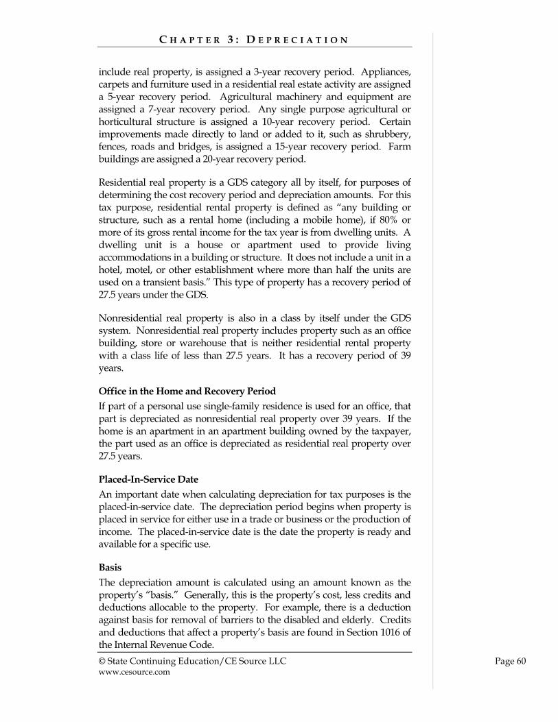
C H A P T E R 3 : D E P R E C I A T I O N
© State Continuing Education/CE Source LLC Page 60 www.cesource.com
include real property, is assigned a 3-year recovery period. Appliances, carpets and furniture used in a residential real estate activity are assigned a 5-year recovery period. Agricultural machinery and equipment are assigned a 7-year recovery period. Any single purpose agricultural or horticultural structure is assigned a 10-year recovery period. Certain improvements made directly to land or added to it, such as shrubbery, fences, roads and bridges, is assigned a 15-year recovery period. Farm buildings are assigned a 20-year recovery period.
Residential real property is a GDS category all by itself, for purposes of determining the cost recovery period and depreciation amounts. For this tax purpose, residential rental property is defined as “any building or structure, such as a rental home (including a mobile home), if 80% or more of its gross rental income for the tax year is from dwelling units. A dwelling unit is a house or apartment used to provide living accommodations in a building or structure. It does not include a unit in a hotel, motel, or other establishment where more than half the units are used on a transient basis.” This type of property has a recovery period of 27.5 years under the GDS.
Nonresidential real property is also in a class by itself under the GDS system. Nonresidential real property includes property such as an office building, store or warehouse that is neither residential rental property with a class life of less than 27.5 years. It has a recovery period of 39 years.
Office in the Home and Recovery Period
If part of a personal use single-family residence is used for an office, that part is depreciated as nonresidential real property over 39 years. If the home is an apartment in an apartment building owned by the taxpayer, the part used as an office is depreciated as residential real property over 27.5 years.
Placed-In-Service Date
An important date when calculating depreciation for tax purposes is the placed-in-service date. The depreciation period begins when property is placed in service for either use in a trade or business or the production of income. The placed-in-service date is the date the property is ready and available for a specific use.
Basis
The depreciation amount is calculated using an amount known as the property’s “basis.” Generally, this is the property’s cost, less credits and deductions allocable to the property. For example, there is a deduction against basis for removal of barriers to the disabled and elderly. Credits and deductions that affect a property’s basis are found in Section 1016 of the Internal Revenue Code.

C H A P T E R 3 : D E P R E C I A T I O N
© State Continuing Education/CE Source LLC Page 61 www.cesource.com
Recovery Periods Under ADS
Under the ADS, property may generally be depreciated over longer recovery periods. Nonresidential real property can be depreciated over 40 years, as can be residential rental property.
Additions and Improvements
Additions and improvements made to depreciable property are treated as separate depreciable property. The recovery period for an addition or improvement begins on the later of:
the date the addition or improvement is placed in service
the date the property to which the addition or improvement was made is placed in service
The recovery period for an addition or improvement is the same as that which would apply to the original property if it had been placed into service at the same time as the addition or improvement.
Depreciation Methods Under MACRS
There are three depreciation methods allowed under GDS, and one depreciation method allowed under ADS:
the 200% declining balance method over a GDS recovery period
the 150% declining balance method over a GDS recovery period
the straight line method over a GDS recovery period
the straight line method over an ADS recovery period

C H A P T E R 3 : D E P R E C I A T I O N
© State Continuing Education/CE Source LLC Page 62 www.cesource.com
Note: The declining balance method is abbreviated as DB and the straight line method is abbreviated as SL.
Method Type of Property Benefit
GSD Using 200% DB
Nonfarm 3-, 5-, 7-, and 10-year property
Provides a greater deduction during the earlier recovery years
Changes to SL when the method provides an equal or greater deduction
GDS Using 150% DB
All farm property (except real property)
All 15- and 20-year property (except qualified leasehold improvement property and qualified restaurant property placed in service before January 1, 2006)
Nonfarm 3-, 5-, 7-, and 10-year property
Provides a greater deduction during the earlier recovery years
Changes to SL when method provides an equal or greater deduction1
GDS Using SL
Nonresidential real property
Qualified leasehold improvement property placed in service before January 1, 2015
Qualified restaurant property placed in service before January 1, 2015
Qualified retail improvement property placed in service before January 1, 2015
Residential rental property
Trees or vines bearing fruit or nuts
Water utility property
All 3-, 5-, 7-, 10-, 15-, and 20-year property
Property for which you elected section 168(k)4
Provides for equal yearly deductions (except for the first and last years)
ADS Using SL
Listed property used 50% or less for business
Property used predominantly outside the US
Tax-exempt property
Tax-exempt bond-financed property
Farm property used when an election not to apply the uniform capitalization rules is in effect
Imported property
Any property for which you elect to use this method 2
Provides for equal yearly deductions (except for the first and last years)
For more details and information go to www.irs.gov

© State Continuing Education/CE Source LLC Page 63 www.cesource.com
Calculating Depreciation Under MACRS
Basically, to calculate depreciation under MACRS using IRS rate tables, the following steps are taken you can use the following worksheet from ths IRS to prepare Form 4562 (not for use for automobiles):
MACRS Worksheet
Part I
1. MACRS system (GDS or ADS)
2. Property class
3. Date placed in service
4. Recovery period
5. Method and convention
6. Depreciation rate (from tables)
Part II
7. Cost or other basis* $
8. Business/investment use %
9. Multiply line 7 by line 8 $
10. Total claimed for section 179 deduction and other items $
11. Subtract line 10 from line 9. This is your tentative basis for depreciation $
12.
Multiply line 11 by .50 if the 50% special depreciation allowance applies. This is your special depreciation allowance. Enter -0- if this is not the year you
placed the property in service, the property is not qualified property, or you elected not to claim a special allowance
$
13. Subtract line 12 from line 11. This is your basis for depreciation
14. Depreciation rate (from line 6)
15. Multiply line 13 by line 14. This is your MACRS depreciation deduction $
*If real estate, do not include cost (basis) of land.
1. Calculate cost or other basis
2. State the percentage of business or investment use of the property
3. Multiply basis by the percentage of business investment use
4. Subtract applicable deductions, such as those for Section 179 deductions
5. This equals tentative basis for depreciation
6. If property was placed into service during the year, calculate the percentage special depreciation allowed for the partial year, if any
7. Subtract the special

C H A P T E R 3 : D E P R E C I A T I O N
© State Continuing Education/CE Source LLC Page 64 www.cesource.com
depreciation allowance (if any) from the tentative basis for depreciation
8. This equals the basis for depreciation
9. Find the depreciation rate for the property from the appropriate IRS table in IRS Publication 946
6. Multiply the depreciation rate by the basis
7. This equals the MACRS depreciation deduction
The following example is found in IRS Publication 946 to show how this is done:
Example.
You bought office furniture (7-year property) for $10,000 and placed it in service on August 11, 2014. You use the furniture only for business. This is the only property you placed in service this year. You did not elect a section 179 deduction and the property is not qualified property for purposes of claiming a special depreciation allowance so your property's unadjusted basis is its cost, $10,000. You use GDS and the half-year convention to figure your depreciation. You refer to the MACRS Percentage Table Guide in Appendix A and find that you should use Table A-1. Multiply your property's unadjusted basis each year by the percentage for 7-year property given in Table A-1. You figure your depreciation deduction using the MACRS worksheet as follows.
MACRS Worksheet
Part I
1. MACRS system (GDS or ADS) GDS
2. Property class 7-year
3. Date placed in service 8/11/14
4. Recovery period 7-Year
5. Method and convention 200%DB/Half-Year
6. Depreciation rate (from tables) .1429
Part II
7. Cost or other basis* $10,000
8. Business/investment use 100 %
9. Multiply line 7 by line 8 $10,000
10. Total claimed for section 179 deduction and other items -0-
11. Subtract line 10 from line 9. This is your tentative basis for depreciation $10,000
12.
Multiply line 11 by .50 if the 50% special depreciation allowance
applies. This is your special depreciation allowance. Enter -0- if this is not the year you placed the property in service, the property is not
qualified property, or you elected not to claim a special allowance
-0-
13. Subtract line 12 from line 11. This is your basis for depreciation $10,000
14. Depreciation rate (from line 6) .1429
15. Multiply line 13 by line 14. This is your MACRS depreciation deduction $1,429
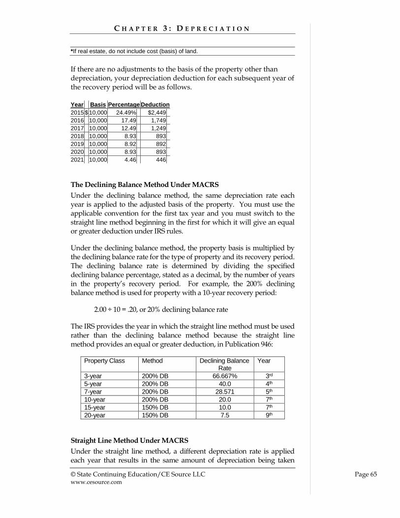
C H A P T E R 3 : D E P R E C I A T I O N
© State Continuing Education/CE Source LLC Page 65 www.cesource.com
*If real estate, do not include cost (basis) of land.
If there are no adjustments to the basis of the property other than depreciation, your depreciation deduction for each subsequent year of the recovery period will be as follows.
Year Basis Percentage Deduction
2015 $ 10,000 24.49% $2,449
2016 10,000 17.49 1,749
2017 10,000 12.49 1,249
2018 10,000 8.93 893
2019 10,000 8.92 892
2020 10,000 8.93 893
2021 10,000 4.46 446
The Declining Balance Method Under MACRS
Under the declining balance method, the same depreciation rate each year is applied to the adjusted basis of the property. You must use the applicable convention for the first tax year and you must switch to the straight line method beginning in the first for which it will give an equal or greater deduction under IRS rules.
Under the declining balance method, the property basis is multiplied by the declining balance rate for the type of property and its recovery period. The declining balance rate is determined by dividing the specified declining balance percentage, stated as a decimal, by the number of years in the property’s recovery period. For example, the 200% declining balance method is used for property with a 10-year recovery period:
2.00 ÷ 10 = .20, or 20% declining balance rate
The IRS provides the year in which the straight line method must be used rather than the declining balance method because the straight line method provides an equal or greater deduction, in Publication 946:
Property Class Method Declining Balance Rate
Year
3-year 200% DB 66.667% 3rd
5-year 200% DB 40.0 4th
7-year 200% DB 28.571 5th
10-year 200% DB 20.0 7th
15-year 150% DB 10.0 7th
20-year 150% DB 7.5 9th
Straight Line Method Under MACRS
Under the straight line method, a different depreciation rate is applied each year that results in the same amount of depreciation being taken

C H A P T E R 3 : D E P R E C I A T I O N
© State Continuing Education/CE Source LLC Page 66 www.cesource.com
each year. The straight line rate is determined by dividing the number 1 by the years remaining in the recovery period at the beginning of that year. If the number of years remaining in the period is less than 1, the depreciation rate for that tax year is 1.0 (1.00%).
MACRS Recovery Periods for Property Used in Rental Activities
Type of Property MACRS Recovery Period
General Depreciation System
Alternative Depreciation System
Computers and their peripheral equipment……….. 5 years 5 years
Office machinery, such as: Typewriters Calculators Copiers …………………………………….. Automobiles …………………………………………. Light trucks ………………………………………….. Appliances, such as Stoves Refrigerators ………………………………. Carpets ………………………………………………. Furniture used in rental property …………………...
5 years 5 years 5 years 5 years 5 years 5 years
6 years 5 years 5 years 9 years 9 years 9 years
Office furniture and equipment, such as: Desks Files ………………………………………... Any property that does not have a class life and that has not been designated by law as being in any other class ………………………………………
7 years 7 years
10 years 12 years
Roads ………………………………………………... Shrubbery …………………………………………… Fences ……………………………………………….
15 years 15 years 15 years
20 years 20 years 20 years
Residential rental property (buildings or structures) And structural components such as furnaces, waterpipes, venting, etc……….
27.5 years
40 years
Additions and improvements, such as a new roof… The same recovery period as that of the property to which the addition or improvements is made, determined as if the property were placed in service at the same time as the addition or improvement.
Depreciation and Appraisals Calculating depreciation is also an important part of some appraisal methods.

C H A P T E R 3 : D E P R E C I A T I O N
© State Continuing Education/CE Source LLC Page 67 www.cesource.com
Depreciation When depreciation is calculated for appraisal purposes, three categories of depreciation are considered and tabulated: physical depreciation, functional depreciation, and economic depreciation.
Physical Depreciation
Physical depreciation is deterioration due to wear and tear and the forces of nature. This type of depreciation can be caused by breakage, infestation by termites, dry rot, negligent care, moisture and elements.
Physical depreciation may be “curable” or “incurable.” Curable depreciation is depreciation that can be remedied by repairing or replacing the defect. Curable physical depreciation is calculated as the cost to cure the defect. Incurable physical depreciation is a condition that if repaired, would have costs that exceed the gain in value from the reparation.
Functional Obsolescence
Functional obsolescence is depreciation that occurs when a structure is unable to perform the function for which it is most used. Functional obsolescence includes things like poor heating, inefficient equipment, poor architecture or floor plans, inadequate room space, etc. The amount of depreciation is the cost to fix the condition, less the value it adds to the property.
Curable functional obsolescence exists when the condition can be categorized as a “normal deficiency,” “modernization,” or “superadequacy.”
Normal Deficiency
“Normal deficiency” is functional obsolescence that requires an addition to the building or other improvement. The depreciation amount is calculated by determining the amount of the addition, and subtracting the original cost.
Modernization
“Modernization” is a deficiency that is curable by modernizing or substituting an item or structure. The depreciation is calculated by determining the original cost of the items to be replaced, less existing wear and tear and salvage, plus the cost to remove old items and replace them with new ones.
Superadequacy
“Superadequacy” is functional obsolescence that occurs because an item provides more function than is adequate for the purpose of the item. The depreciation is calculated by determining the cost of removing and

C H A P T E R 3 : D E P R E C I A T I O N
© State Continuing Education/CE Source LLC Page 68 www.cesource.com
replacing the item, or the cost of altering it, so that the item is performing its proper, adequate function.
Economic Obsolescence
Economic obsolescence is also known as “external obsolescence.” Economic obsolescence exists because of an external cause, such as where the property is located, a change of zoning, a change in tax treatment, etc. The depreciation is calculated by capitalizing the income or rent loss caused by the economic or external factor, or by making a negative adjustment based on the value of comparable properties, where some of the comparable properties are affected by the same factors, and some are not.
Depreciation and Time
When calculating depreciation, there are three important time periods used – the effective age of the property, the remaining economic life of the property, and the total economic life of the property.
Effective Age
The effective age of subject property is the number of years of age based on the condition of the property. For example, all the homes in a subdivision were built within months of one another. The homes in average condition are assigned an effective age equal to the number of years since they were constructed. The homes in excellent condition are assigned effective ages less than the number of years since they were constructed. The homes in poor condition are assigned effective ages greater than the number of years since they were constructed.
Remaining Economic Life
The remaining economic life of a property is the estimated period of time in which improvements will add to the value of the property. Factors the appraiser takes into consideration to determine this figure include the current condition of the building, future zoning and similar factors that may add or detract to value, the general desirability of the type of property over time, the location of the property, the growth pattern and economic vitality of the area.
Total Economic Life
The total economic life of a property is the total of the effective age and the remaining economic life of a property. The effective life of a property is constrained by its highest and best use.
Economic Life Example 1
The home has an effective age of 7 years. It has a remaining economic life of 20 years. Its total economic life is effective age + economic life, or 7 years + 20 years = 27 years.

C H A P T E R 3 : D E P R E C I A T I O N
© State Continuing Education/CE Source LLC Page 69 www.cesource.com
Economic Life Example 2
The home has a total economic life of 40 years. It has an effective age of 12 years. What is its remaining economic life?
Total economic life – effective life = remaining economic life
40 years – 12 years = 28 years
Calculating Depreciation
For appraisal purposes, there are six methods of calculating depreciation. These are:
1. Capitalization of Income
2. Depreciation Tables
3. Economic Age-Life
4. Modified Economic Age-Life
5. Observed Condition (Breakdown)
6. Sales Comparison
Capitalization of Income
The capitalization of income method, which is used to value various types of income producing business properties, involves determining a capitalization rate derived from the reproduction cost of the structure. The capitalization rate is normally found by the following formula, when properties have a known value:
Net Income = Capitalization Rate or I = R Value of Property V
When the value is not known in a capitalization rate equation, the following formula is used:
Net Income = Value of Property or I = V Capitalization Rate R
When the net operating income is not known, such as when analyzing a prospective income producing property, the following formula is used:
Value of Property x Capitalization Rate = Net Operating Income
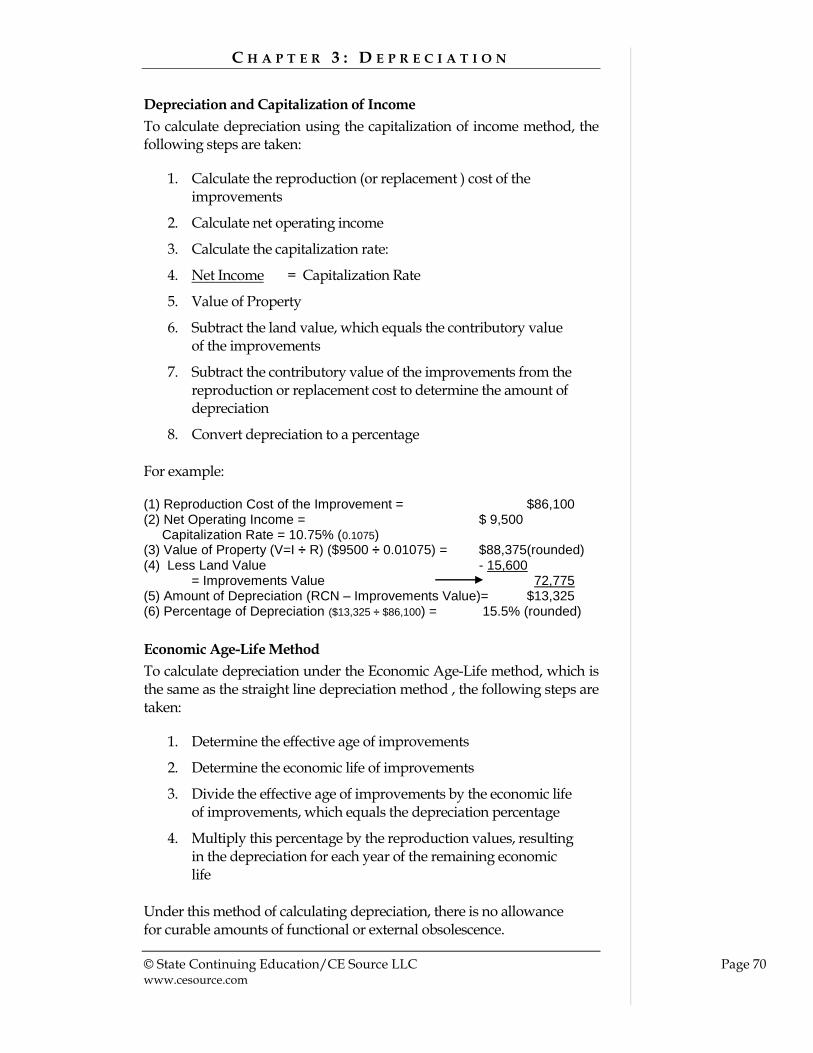
C H A P T E R 3 : D E P R E C I A T I O N
© State Continuing Education/CE Source LLC Page 70 www.cesource.com
Depreciation and Capitalization of Income
To calculate depreciation using the capitalization of income method, the following steps are taken:
1. Calculate the reproduction (or replacement ) cost of the improvements
2. Calculate net operating income
3. Calculate the capitalization rate:
4. Net Income = Capitalization Rate
5. Value of Property
6. Subtract the land value, which equals the contributory value of the improvements
7. Subtract the contributory value of the improvements from the reproduction or replacement cost to determine the amount of depreciation
8. Convert depreciation to a percentage
For example:
(1) Reproduction Cost of the Improvement = $86,100 (2) Net Operating Income = $ 9,500 Capitalization Rate = 10.75% (0.1075) (3) Value of Property (V=I ÷ R) ($9500 ÷ 0.01075) = $88,375(rounded) (4) Less Land Value - 15,600
= Improvements Value 72,775 (5) Amount of Depreciation (RCN – Improvements Value)= $13,325 (6) Percentage of Depreciation ($13,325 ÷ $86,100) = 15.5% (rounded)
Economic Age-Life Method
To calculate depreciation under the Economic Age-Life method, which is the same as the straight line depreciation method , the following steps are taken:
1. Determine the effective age of improvements
2. Determine the economic life of improvements
3. Divide the effective age of improvements by the economic life of improvements, which equals the depreciation percentage
4. Multiply this percentage by the reproduction values, resulting in the depreciation for each year of the remaining economic life
Under this method of calculating depreciation, there is no allowance for curable amounts of functional or external obsolescence.

C H A P T E R 3 : D E P R E C I A T I O N
© State Continuing Education/CE Source LLC Page 71 www.cesource.com
Example of Economic Age-Life Method
For example, the effective age of improvement is 5 years. The economic life of the improvement is 40 years. The reproduction value is $585,000. The depreciation amount is:
5 years = .125 .125 X $585,000 = $73,125 40 years
Modified Age-Life Method
The difference between the Economic Age-Life method and the Modified Age-Life method is that the depreciation amounts for curable physical deterioration and functional obsolescence are subtracted from the reproduction (or replacement) cost of the improvements under the Modified method. The remaining value is used to determine the amount of depreciation over the remaining economic life of the property.
Observed Condition Method
The observed condition method of calculating depreciation requires categorizing and listing each cause of depreciation and adding them together:
Physical Deterioration
Curable $
Incurable $
Functional Obsolescence
Curable $
Incurable $
External Obsolescence
Curable $
Incurable $
TOTAL $$

C H A P T E R 3 : D E P R E C I A T I O N
© State Continuing Education/CE Source LLC Page 72 www.cesource.com
For example:
Physical Deterioration
Curable $50,000
Incurable $ 00
Functional Obsolescence
Curable $12,000
Incurable $ 00
External Obsolescence
Curable $ 00
Incurable $ 00
TOTAL $62,000
Using Depreciation Tables
There are depreciation tables that can be used by appraisers to calculate deprecation. These tables provide schedules of typical value standards for determining depreciation. Tables are available that reflect regional conditions.
Sales Comparison Method of Depreciation
Under the sales comparison method of depreciation, the depreciation value in comparable properties is found and the depreciation percentage of the property value is determined. This percentage is applied to the subject property’s value to find its depreciation amount:
1. Find the sales price of the comparable property
2. Subtract the land value from the sales price to equal the depreciated value of the improvements
3. Divide the depreciated value of the improvements by the age of the improvements to find the depreciation rate per year
4. Multiply the depreciation rate per year by the subject property’s age in years to find the depreciation rate for the subject property
5. Multiply the subject’s depreciation rate by its reproduction cost to equal the depreciation for the subject property
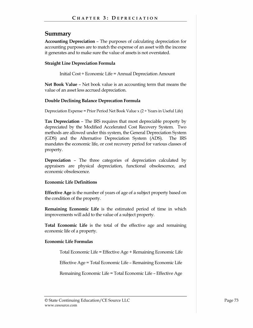
C H A P T E R 3 : D E P R E C I A T I O N
© State Continuing Education/CE Source LLC Page 73 www.cesource.com
Summary Accounting Depreciation – The purposes of calculating depreciation for accounting purposes are to match the expense of an asset with the income it generates and to make sure the value of assets is not overstated.
Straight Line Depreciation Formula
Initial Cost ÷ Economic Life = Annual Depreciation Amount
Net Book Value – Net book value is an accounting term that means the value of an asset less accrued depreciation.
Double Declining Balance Deprecation Formula
Depreciation Expense = Prior Period Net Book Value x (2 ÷ Years in Useful Life)
Tax Depreciation – The IRS requires that most depreciable property by depreciated by the Modified Accelerated Cost Recovery System. Two methods are allowed under this system, the General Depreciation System (GDS) and the Alternative Depreciation System (ADS). The IRS mandates the economic life, or cost recovery period for various classes of property.
Depreciation – The three categories of depreciation calculated by appraisers are physical depreciation, functional obsolescence, and economic obsolescence.
Economic Life Definitions
Effective Age is the number of years of age of a subject property based on the condition of the property.
Remaining Economic Life is the estimated period of time in which improvements will add to the value of a subject property.
Total Economic Life is the total of the effective age and remaining economic life of a property.
Economic Life Formulas
Total Economic Life = Effective Age + Remaining Economic Life
Effective Age = Total Economic Life – Remaining Economic Life
Remaining Economic Life = Total Economic Life – Effective Age
C H A P T E R 3 : D E P R E C I A T I O N
© State Continuing Education/CE Source LLC Page 74 www.cesource.com

© State Continuing Education/CE Source LLC Page 75 www.cesource.com
CHAPTER FOUR
RREEAALL EESSTTAATTEE TTAAXXEESS
There may be a variety of taxes paid on real estate. This chapter will discuss how to calculate real estate taxes.
Upon completion of this chapter, you will be able to:
Calculate taxes using mills
Calculate special assessments
Explain documentary stamp tax
Explain the Texas Homestead exemption
Tax Assessed Value Property taxes are calculated by determining the value according to the tax laws of the area in which the real estate is located. Tax assessors value the property using generally the same principles of valuation as the professional appraiser. However, tax values are limited by provisions in tax law. For example, the maximum amount of an annual increase in assessed value may be capped in the tax law. Or, a property may qualify as a “homestead” under the tax law, and the property’s value reduced due to the homestead exemption. For example, the state gives each property that qualifies as a homestead a $25,000 exemption, which is subtracted from the assessed value. Then, the tax rate is applied to this reduced, or taxable, value.
Texas Homestead Exemption
In Texas, a residence homestead exemption applies to a property’s assessed value. The definition of a residence homestead is “a structure (including a mobile home) or a separately secured and occupied portion of a structure (together with the land), not to exceed 20 acres, and improvements used in the residential occupancy of the structure if the structure and the land and improvements have identical ownership that:

C H A P T E R 4 : R E A L E S T A T E T A X E S
© State Continuing Education/CE Source LLC Page 76 www.cesource.com
A. is owned by one or more individuals, either directly or through a beneficial interest in a qualifying trust;
B. is designed or adapted for human residence;
C. is used as a residence; and
D. is occupied as his principal residence by an owner, or, for property owned through a beneficial interest in a qualifying trust, by a trustor of the trust who qualifies for the exemption.”
Effective January 1, 2016, the exemption amount for a residence homestead against assessed value is $25,000 for taxes assessed by a school district. An adult who is disabled or is 65 or older is entitled to an additional exemption of $10,000. Also, Texas law provide partial exemptions for property owned by disabled veterans and surviving spouses (not remarried) and children of deceased disabled veterans. Additional exemptions may apply to other taxing authorities’ assessed values.
Tax Rates For property tax purposes, the tax rate is stated in the form of “mills.” A mill is 1/1000th of a dollar, or $.001. There are 1000 mills in a dollar. A tax rate shown as $.015 is 15 mills per dollar.
The tax rate is 25 mills per dollar. Here are equivalent ways of stating this value:
25 mills per $1 of assessed value
$.025 mills per $1 of assessed value
$2.50 per $100 of assessed value
$25 per $1000 of assessed value
Calculating Property Taxes Typically, the taxing entity for property taxes is the county or the city. The taxing entity calculates the tax due by applying the appropriate tax rate to the assessed value.
The property’s assessed value is $100,000. The tax rate is $.020 mills per $1 of assessed value. The tax is $100,000 X $.020 = $2000.
More Than One Tax Rate
There may be different tax rates assessed on the same property by different taxing authorities. For example, the city may have a tax rate of 6

C H A P T E R 4 : R E A L E S T A T E T A X E S
© State Continuing Education/CE Source LLC Page 77 www.cesource.com
mills per $1000 on the property, and the county may have a tax rate of 16 mills per $1000 on the property. The property’s assessed value is $239,000. The total property taxes are:
City taxes = $.006 X $239,000 = $1434
County taxes = $.016 X $239,000 = $3824
Total taxes are $1434 + $3824 = $5258
Special Assessments
Assessments are taxes that are charged by a municipality or other taxing authority for special purposes, such as road improvements, sewers, a library, the firefighters and police, etc. These assessments may be charged on the full size of the property, on the frontage, or on the assessed value of the property for county property tax purposes. For example, if the assessment is for a road improvement, or city sewers, the assessment may be based on the frontage. If the sewer assessment is $7.5 per foot of frontage, and the property owner has 200 feet of frontage, this property owner must pay $1500:
$7.5 x 200 front feet = $1500
Documentary Stamp Tax A Documentary Stamp Tax is levied when a “stamp” or imprint is placed on documents, such as a deed, by the state. The tax is on the purchase price paid for the property and is payable by the seller. The tax is generally stated as a rate per $100 of the purchase price. For example, the documentary stamp tax is $.70 per $100. The purchase price is $279,000. The tax is: $279,000 X $.70 = $1953 $100
If dividing the purchase price by $100 to find the tax base results in a fractional portion, the fractional portion is rounded to the next whole number. For example:
1. The purchase price is $175,939
The tax base is $175,939 = $1759.39 = $1760 tax base $100
The tax is $1760 X $.70 = $1232
2. The purchase price is $137,229
The tax base is $137,229 = $1372.29 = $1373 tax base $100

C H A P T E R 4 : R E A L E S T A T E T A X E S
© State Continuing Education/CE Source LLC Page 78 www.cesource.com
The tax is $1373 X $.70 = $961.10
Texas does not have a documentary stamp tax.
Summary Taxes on real property are charged on the assessed value. There may be exemptions from value, such as a homestead residence exemption.
Mills – Tax rates are stated in “mills.” A mill is 1/1000th of a dollar.
Equivalents:
10 mills per $1 of assessed value
$0.010 mills per $1 of assessed value
$1.00 per $100 of assessed value
$10 per $1000 of assessed value
Formula for calculating taxes
Tax = Tax Rate X Assessed Value
Special Assessments = Tax Rate x Assessed Value
Or
Tax Rate x Property Size
Documentary Stamp Tax – This tax rate is stated as a rate per $100 of the purchase price of property.
Tax = (Purchase Price ÷ $100) X Tax Rate

© State Continuing Education/CE Source LLC Page 79 www.cesource.com
CHAPTER FIVE
CCLLOOSSIINNGG CCAALLCCUULLAATTIIOONNSS
Closing or settlement is the finalization of a real estate transaction. It involves many financial calculations. Costs that are calculated and settled at this time include:
Appraisal fees
Loan origination fees
Loan discount fees, if any
Loan underwriting fees
Credit report fees
Tax service fees
Documentation fees
Title insurance premiums
Recording fees
Settlement or closing fees
These costs are usually a flat fee or a percentage of the loan.
Other costs that are calculated at closing are more complicated to determine. For example, property taxes, mortgage interest and rental income may all need to be prorated between the buyer and seller. Calculating proration amounts was discussed in Chapter Two, and will be further discussed in this chapter.
Upon completion of this chapter, you will be able to:
Explain debits and credits as used in a closing statement
Prorate property taxes
Prorate mortgage interest
Prorate prepaid rent
Explain the use and format of the new Closing Disclosure
Calculate and record items in the closing process

C H A P T E R 5 : C L O S I N G C A L C U L A T I O N S
© State Continuing Education/CE Source LLC Page 80 www.cesource.com
Completing Closing Calculations The closing process includes all the financial data from the real estate transaction. Amounts owed by the buyer are debited to the buyer, and amounts due the buyer are credited to the buyer. Amounts owed by the seller are debited to the seller, and amounts due the seller are credited to the seller. Debits take money away from the party. Credits give money to the party.
Credits to the Buyer
The following items are normally credits to the buyer:
Earnest money, paid by the buyer
An assumed loan balance, if any
Prorations for items such as property taxes, prepaid rents and mortgage interest that the seller owes the buyer
New loan proceeds
Credits to the Seller
Credits to the seller generally include:
The sales price of the property
Items prepaid by the seller that the buyer owes the seller for, such as insurance or fuel on hand
Non-Balancing Entries
Items such as prorations are entered as a debit to one party and a credit to the other. Other items are entered only as a credit or debit to one party. Seller’s expenses are debits to the seller only. They are not credited to the buyer, but will be disbursed to others by the settlement agent. These include the broker’s commission, repairs, loan pay-off fees, and other fees the seller may have agreed to pay in the sales contract.
Items debited to the buyer only may include fees for inspections, the appraisal fee, mortgage insurance premiums, credit report fee, loan origination fee, recording fees to record the deed and the mortgage and homeowners insurance and flood insurance premiums.
Some expenses are agreed to be shared by the buyer and seller, and so a portion is debited to each. These expenses may include fees for title insurance, escrow, inspections, and legal fees.

C H A P T E R 5 : C L O S I N G C A L C U L A T I O N S
© State Continuing Education/CE Source LLC Page 81 www.cesource.com
Prorations Items such as property taxes, mortgage interest and rental income must be prorated during the closing process.
Property Taxes
The buyer becomes responsible for the payment of property taxes on the property from the day of closing forward. The seller is responsible for their payment up to the day of closing. Property taxes are usually due at the end of the period for which they are calculated, so are paid in “arrears.”
For example, property taxes are calculated for the period of November 1, 2007 through October 31, 2008, and are due by November 30, 2008. If closing takes place on March 31, 2008, the seller is responsible for the property tax amount attributable to the period November 1, 2007 to March 30, 2008.
The buyer is responsible for the taxes from March 31 – October 31, 2008, and from then on until the buyer sells the property.
Prorating Property Taxes Example
Here is an example of this type of calculation: Property taxes are charged from January 1 to December 31 by the county. They are due 15 days after the end of this period. The total property taxes are $2,050. The home is sold during this period and closes on August 31. The seller owes the taxes from January 1 to August 30. The buyer owes the taxes for this period from August 31 to December 31. To prorate this amount, calculate the number of days for which each party is responsible to pay the taxes and the daily rate for the tax, and multiply the number of days times the daily rate:
Daily property tax amount = $1898 ÷ 365 = $5.20
Seller’s Days Responsible for Tax =
January 31 days
February 28 days
March 31 days
April 30 days
May 31 days
June 30 days

C H A P T E R 5 : C L O S I N G C A L C U L A T I O N S
© State Continuing Education/CE Source LLC Page 82 www.cesource.com
July 31 days
August 30 days
Total Days 242 days
242 days X $5.20 = $1258.40 = Seller’s Amount
Buyer’s Days Responsible for Tax =
August 1 day
September 30 days
October 31 days
November 30 days
December 31 days
Total Days 123 days
123 Days X $5.20 = $639.60 = Buyer’s Amount
The seller’s amount of $1258.40 is credited to the buyer at closing, since the buyer will be paying the entire bill after the end of the year. It is debited to the seller, because the seller owes it to the buyer.
Sample Settlement Statement Excerpt
Prorations Buyer’s Transactions Seller’s Transactions
Debit Credit Debit Credit
Prepaid Tax $1258.40 $1258.40
Mortgage Interest
Mortgage interest is also generally paid at the end of the period for which it is charged, or in arrears. The period is usually a month. The seller is responsible for the interest and payment to the date of closing. The buyer’s mortgage starts on the date of closing. An example of prorating interest in an assumed mortgage was given in Chapter Two. Here is another example:
Prorating Mortgage Interest Example
The seller’s mortgage is being assumed by the buyer at closing. The amount of this mortgage is $42,506 through April 30, and the rate is 6.2%. Closing is scheduled for May 21. Calculate the prorated interest for May:

C H A P T E R 5 : C L O S I N G C A L C U L A T I O N S
© State Continuing Education/CE Source LLC Page 83 www.cesource.com
Step 1: Calculate the annual interest based on the current principal balance:
$42,506 X 6.2% = $2635.37
Step 2: Calculate the daily interest:
$2635.37 ÷ 365 = $7.220191781
Step 3: Calculate the seller’s interest due the buyer:
Seller owes May 1 – May 20 = 20 days X $7.220191781 = $144.40
This amount is entered as a debit to the seller on the closing statement, and a credit to the buyer:
Sample Settlement Statement Excerpt
Prorations Buyer’s Transactions Seller’s Transactions
Debit Credit Debit Credit
Mortgage Interest
$144.40 $144.40
Prepaid Rent
A property used as a rental may have prepaid rental amounts. For example, the seller of the property may have required the renter to pay the last month’s rent at the time of leasing the property. This amount is prepaid rent. Rent is usually charged at the beginning of each period on a month-to-month lease. This is also prepaid rent.
For example, rent for the home is $900 per month, payable at the beginning of the month. The home is sold with a closing date of June 15. The seller earns the monthly rent from June 1 to June 14. The buyer earns the monthly rent from June 15 to June 30.
Calculating the proration amount using daily interest based on the 30 days in June is done as follows:
$900 ÷ 30 days = $30 per day
Seller’s rental income = June 1 to June 14 = 14 days X $30 = $420
Buyer’s rental income = June 15 to June 30 = 16 days X $30 = $480
Because the seller has already collected the total $900 rent, the seller owes the buyer $480. On the closing statement, this amount would be shown as a credit to the buyer, and a debit to the seller:

C H A P T E R 5 : C L O S I N G C A L C U L A T I O N S
© State Continuing Education/CE Source LLC Page 84 www.cesource.com
Sample Settlement Statement Excerpt
Prorations Buyer’s Transactions Seller’s Transactions
Debit Credit Debit Credit
Prepaid Rent $480 $480
Disclosures and Sample Forms Effective October 3, 2015, the Consumer Financial Protection Bureau issued a new rule that consolidates the mortgage disclosures established by the Truth-in-Lending Act (TILA) and the Real Estate Settlement Procedures Act (RESPA) into a single rule.
The Uniform Settlement Statement, also known as the HUD-1 Settlement Statement and the final Truth-in-Lending Statement, were replaced by the Closing Disclosure. These changes apply to most consumer mortgage loans for 1-4 unit dwellings that are attached to real property. It does NOT apply to home-equity lines of credit, reverse mortgage loans, mortgage loans secured by a mobile home or by a dwelling not attached to real property. It also does not apply to creditors that write five or less mortgages a year. There will also be a partial exemption given to junior liens when they are associated with housing assistance loans for low to moderate income consumers.
A sample of this form follows:

C H A P T E R 5 : C L O S I N G C A L C U L A T I O N S
© State Continuing Education/CE Source LLC Page 85 www.cesource.com
Closing Disclosure Sample Page 1 (http://files.consumerfinance.gov/f/201311_cfpb_kbyo_closing-disclosure.pdf)

C H A P T E R 5 : C L O S I N G C A L C U L A T I O N S
© State Continuing Education/CE Source LLC Page 86 www.cesource.com
Closing Disclosure Sample Page 2 (http://files.consumerfinance.gov/f/201311_cfpb_kbyo_closing-disclosure.pdf)

C H A P T E R 5 : C L O S I N G C A L C U L A T I O N S
© State Continuing Education/CE Source LLC Page 87 www.cesource.com
Closing Disclosure Sample Page 3 (http://files.consumerfinance.gov/f/201311_cfpb_kbyo_closing-disclosure.pdf)
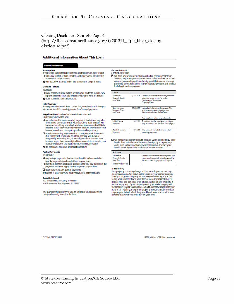
C H A P T E R 5 : C L O S I N G C A L C U L A T I O N S
© State Continuing Education/CE Source LLC Page 88 www.cesource.com
Closing Disclosure Sample Page 4 (http://files.consumerfinance.gov/f/201311_cfpb_kbyo_closing-disclosure.pdf)

C H A P T E R 5 : C L O S I N G C A L C U L A T I O N S
© State Continuing Education/CE Source LLC Page 89 www.cesource.com
Closing Disclosure Sample Page 5 (http://files.consumerfinance.gov/f/201311_cfpb_kbyo_closing-disclosure.pdf)
Other Settlement Statement Forms When a Closing Disclosure isn’t required, the closing statement format may vary, depending on the Settlement company. The statement format may include a four column section, similar to the example used in this
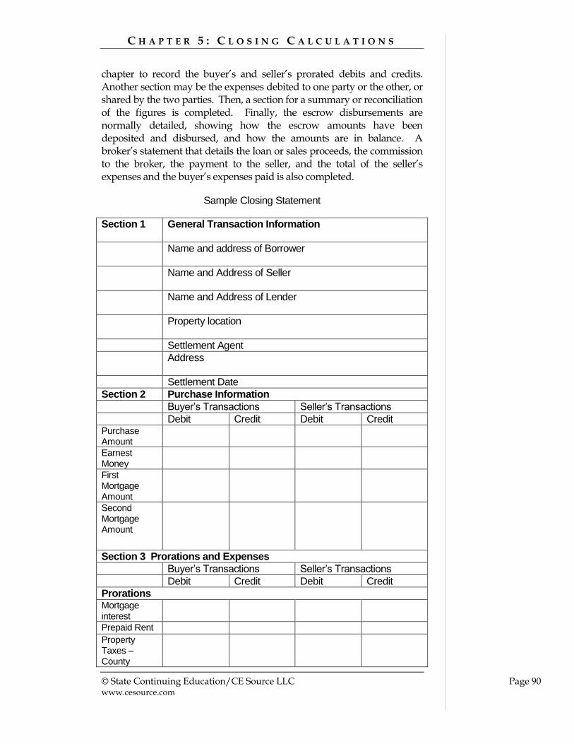
C H A P T E R 5 : C L O S I N G C A L C U L A T I O N S
© State Continuing Education/CE Source LLC Page 90 www.cesource.com
chapter to record the buyer’s and seller’s prorated debits and credits. Another section may be the expenses debited to one party or the other, or shared by the two parties. Then, a section for a summary or reconciliation of the figures is completed. Finally, the escrow disbursements are normally detailed, showing how the escrow amounts have been deposited and disbursed, and how the amounts are in balance. A broker’s statement that details the loan or sales proceeds, the commission to the broker, the payment to the seller, and the total of the seller’s expenses and the buyer’s expenses paid is also completed.
Sample Closing Statement
Section 1
General Transaction Information
Name and address of Borrower
Name and Address of Seller
Name and Address of Lender
Property location
Settlement Agent
Address
Settlement Date
Section 2 Purchase Information
Buyer’s Transactions Seller’s Transactions
Debit Credit Debit Credit Purchase Amount
Earnest Money
First Mortgage Amount
Second Mortgage Amount
Section 3 Prorations and Expenses
Buyer’s Transactions Seller’s Transactions
Debit Credit Debit Credit
Prorations Mortgage interest
Prepaid Rent Property Taxes – County

C H A P T E R 5 : C L O S I N G C A L C U L A T I O N S
© State Continuing Education/CE Source LLC Page 91 www.cesource.com
Property Taxes – City
Other
Expenses Broker’s Commission
Repairs Loan Pay-Off Fees
Inspections Appraisal Fees
Mortgage Insurance Premiums
Credit Report Fee
Loan Origination Fee
Recording Fees
Hazard Insurance
Flood Insurance
Title Insurance
Escrow Fees Legal Fees Other
Section 4 Total Debits and Credits
TOTALS
Balance Due to Seller
Balance Due From Buyer
Broker’s Statement
Receipts Disbursements
Earnest Money $$
Check from Buyer $$
Broker’s Commission $$
Check to Seller $$
Seller’s Expenses $$
Buyer’s Expenses $$
TOTALS $$$$ $$$$

C H A P T E R 5 : C L O S I N G C A L C U L A T I O N S
© State Continuing Education/CE Source LLC Page 92 www.cesource.com
Summary Debits and Credits – At closing, amounts owed by the seller are debited to the seller, and amounts due the seller are credited to the seller. Amounts owned by the buyer are debited to the buyer, and amounts due the buyer are credited to the seller. Debits take money away from a party. Credits give money to a party.
Prorations – Prorations are amounts debited and credited to the buyer and seller for items that the seller either owes to the buyer, or items the buyer owes the seller. These may include prepaid rents, property taxes and mortgage interest under an assumed mortgage.
Prorating Property Tax Formulas
Daily Property Tax Rate = Total Property Tax ÷ 365
Seller’s Debit/Buyer’s Credit for Property Taxes = # of Days in Tax Year Prior to Closing x Daily Property Tax Rate
Prorating Prepaid Rent Formulas
Daily Prepaid Rent Rate = Total Prepaid Rent ÷ # of Days in Month
Seller’s Debit/ Buyer’s Credit for Prepaid Rent = # of Days from Closing to end of Month X Daily Prepaid Rent Rate
Prorating Mortgage Interest Formulas
Annual Mortgage Interest = Current Loan Principal X Mortgage Rate
Monthly Mortgage Interest = Annual Mortgage Interest ÷ 12
Daily Mortgage Interest = Monthly Mortgage Interest ÷ # of days in Month of Closing
Seller’s Debit / Buyer’s Credit = # of Days from beginning of Month through the day before closing x Daily Mortgage Interest

© State Continuing Education/CE Source LLC Page 93 www.cesource.com
GGLLOOSSSSAARRYY
203(b): A FHA insurance program that provides mortgage insurance to protect lenders from default for loans used to finance the purchase of new or existing one- to four family housing, with a low down payment, flexible qualifying guidelines, limited fees, and a limit on maximum loan amounts.
203(k: A FHA insurance program that provides mortgage insurance to protect lenders from default for loans used to finance both the purchase of a house and the cost of its rehabilitation through a single mortgage loan.
Appraisal: A written statement that is independently and impartially prepared by a qualified appraiser that sets forth an opinion of defined value of a property as of a specific date, supported by the presentation and analysis of market information.
Appraisal Report: A written report, independently and impartially prepared, that sets forth an opinion of defined value of a property, as of a specific date, and supported by the presentation and analysis of market data Appraiser: A professional who uses his or her experience and knowledge to prepare the appraisal estimate.
Basis: A measure of an individual’s investment in property for tax and accounting purposes. Capitalization: Converting a series of anticipated future payments into present value. Capitalization transforms net operating income produced by a property into the property value. Capitalization Rate: A composite rate used for converting property income into property value. Conventional Loan: A loan that is made through the private market sector and is not guaranteed or insured by the U.S. government.
Curable Depreciation: Items of physical deterioration and functional obsolescence which are customarily repaired or replaced by a prudent property owner. Depreciation: Loss of value of property brought about by age, physical deterioration or functional or economic obsolescence. Down payment: The portion of a home's purchase price paid in cash.

G L O S S A R Y
© State Continuing Education/CE Source LLC Page 94 www.cesource.com
Economic Life: The period over which a property will yield a return on the investment. Economic Obsolescence: A loss in value due to external factors that adversely affect the value of the subject property. Effective Age: The number of years of age indicated by the condition of the structure. Eminent Domain: The power to take private property for public use by the state and municipalities. Fee Simple Estate: The greatest interest that one can have in real property. An estate that is unqualified, of indefinite duration, freely transferable and inheritable. Frontage: A term used to describe or identify that part of a parcel of land or an improvement on the land which faces a street, or a view, or amenity such as a lake. Functional Obsolescence : A loss of value due to adverse factors from within the structure which affect the utility of the structure, value and marketability. Highest And Best Use: The highest value that a property is capable of attaining at the time of appraisal considering the legally permitted use; financially feasible; maximum profitability of the land/or buildings over a given period; and physically possible. Improvement: Refers to additions to or betterments of real property that enhance its value and are designed to make the property more useful or valuable. Life Estate: A possessory, freehold estate in land held by a person only for the duration of his or her life or the life or lives of another. Metes And Bounds: A term used in describing the boundary lines of land, setting forth all the boundary lines together with their terminal points and angles. Mortgage: A lien on the property that secures the promise to repay a loan.
Mortgage Insurance: Insurance that protects lenders against some or most of the losses that can occur when a borrower defaults on a mortgage loan.

G L O S S A R Y
© State Continuing Education/CE Source LLC Page 95 www.cesource.com
Net Income: The money remaining after expenses are deducted from income; the profit. Private Mortgage Insurance (PMI): Privately issued insurance for qualified borrowers with down payments of less than 20% of a purchase price.
Replacement Cost: The cost to replace a structure with one having utility equivalent to that being appraised, but constructed with modern materials and according to current standards, design and layout. Reproduction Cost: The cost of replacing the subject improvement with one that is the exact replica, having the same quality of workmanship, design and layout, or cost to duplicate an asset. Township: In the survey of public lands of the United States, a territorial subdivision six miles long, six miles wide and containing 36 sections, each one mile square, located between two range lines and two township lines. Zoning: An act of city or county officials that specifies the type of use to which property may be put in specific areas.

© State Continuing Education/CE Source LLC Page 96 www.cesource.com
INDEX
A
Acres, 5, 6, 20
Amortization, 46, 47, 48, 49
Appraisal, 92
Appraisals, 65
Area, 2, 4, 6, 7, 8, 9
Assessments, 84, 85
Assumption, 86
C
Calculators, 26
Closing
Credits, 78, 81, 82, 83, 86, 89,
90
Debits, 81, 82, 83, 89
Commission, 27, 28, 29, 30, 86,
89, 90
Credit, 86
Cubic Measurement, 9, 10
D
Debt to Income Ratio, 43
Default, 41
Depreciation, 25, 53, 54, 56, 57,
59, 61, 63, 65, 67, 68, 69, 71,
92
Economic Obsolescence, 67, 93
Functional Obsolescence, 66,
70, 71, 93
Physical, 66
Straight Line, 54, 55, 56, 57
Down Payments, 39
E
Effective Age, 67, 93
F
Fannie Mae, 43
Fee Simple, 93
Foreclosure, 41
Freddie Mac, 43
Front Feet, 6
H
Homestead Exemption, 74
HUD-1 Settlement Statement, 78,
83, 84, 88
I
Interest, 23, 31, 32, 33, 35, 44, 45,
46, 47, 50, 51, 81, 82, 86
Annual, 33
Compound, 36, 37
Monthly, 33
Quarterly, 33
Simple, 32
Time, 31, 32, 67
L
Legal Descriptions, 12, 17
Blocks and Lots, 16
Metes-and-Bounds, 13
Plats, 17
U.S. Government Survey
System, 1, 17
Life Estate, 93
Loan Commitment Fees, 42
Loan Discount Points, 42
Loan Origination Fees, 42
Loan Payment to Income Ratio,
43
Loan Principal, 47
Loan-to-Value, 40, 41
M
Metric, 10
Modified Accelerated Cost
Recovery System, 59
Mortgage, 41
Mortgage Insurance, 41, 42, 84,
86, 90, 93, 94

I N D E X
© State Continuing Education/CE Source LLC Page 97 www.cesource.com
N
Net Book Value, 56, 57
Net Operation Income, 68, 69
P
Percentages, 24, 30
Perimeter, 2
PITI, 50
Prepaid Rent, 81, 82, 83, 89
Principal, 32, 33, 44, 47, 50, 51,
84
Property Taxes, 75, 80, 89
Prorating, 23, 33, 78, 80, 81
R
Rate of Return, 30, 31
Rectangles, 2
Remaining Economic Life, 67
S
Salvage, 54
Settlement Statements, 81, 82, 83,
88
Squares, 3
Straight Line Depreciation, 54,
55, 56, 57
T
Tax Assessed Value, 74
Title, 87
Total Economic Life, 67
Triangles, 7
U
U.S. Government Survey System
Sections, 18
V
Veterans Administration, 43
Volume, 9, 10