understanding r-process nucleosynthesis in the milky way
TRANSCRIPT

Understanding r-process Nucleosynthesis inthe Milky Way
Author:
Christopher HAYNES
Supervised by:
Dr. C. KOBAYASHI
Centre for Astrophysics Research
School of Physics, Astronomy and Mathematics
University of Hertfordshire
Submitted to the University of Hertfordshire in partial fulfilment of the requirements of
the degree of Doctor of Philosophy.
September 2019

Abstract
Elements heavier than Fe are formed by neutron capture processes when fusion becomes en-
ergetically unfavourable; the slow s-process and site are reasonably well understood, but the
rapid r-process site is still a highly debated topic. In this thesis I will discuss the current best
understanding of both the s-process and r-process, including potential sites. I also discuss the
modelling of galaxies using smoothed particle hydrodynamics simulations with the inclusion of
nucleosynthesis models to simulate the chemical evolution of galaxies. I then present the results
of such chemodynamical simulations including nucleosynthesis yields for neutron star mergers,
magneto-rotational supernovae, electron capture supernovae and neutrino driven winds. Using
the [Eu/(Fe,α)] - [Fe/H] relation I show the neutron star mergers are unlikely to be able to drive
r-process enrichment in the early universe but that magneto-rotational supernovae, or a combi-
nation of sources including them, may be able to. I then include a metallicity dependence in the
magneto-rotational supernova model, and show that a combined model with neutron star merg-
ers and electron-capture supernovae gives an excellent match to observations of [(Eu, Nd, Dy,
Er, Zr)/(Fe, α)]. Finally I discuss the effects of supernova feedback on chemical evolution. I
compare four models: a thermal model, a thermal model with a kinetic component, a stochastic
model and a mechanical model and show that the kinetic, stochastic and mechanical models can
suppress the star formation within isolated dwarf disc galaxies when using optimal parameters
and that this has little effect on the fraction of metals ejected from the galaxy.

Declaration
I declare that no part of this work is being submitted concurrently for another award of the
University or any other awarding body or institution. This thesis contains a substantial body of
work that has not previously been submitted successfully for an award of the University or any
other awarding body or institution.
The following parts of this submission have been published previously and/or undertaken as part
of a previous degree or research programme:
1. Chapter 4: This chapter has been accepted and published as Haynes & Kobayashi 2019 in
Monthly Notices of the Royal Astronomical Society, Volume 483, Issue 4, March 2019,Pages 5123 - 5134
2. Chapter 5: This chapter is a completed paper at the time of writing and due to be submitted
to Monthly Notices of the Royal Astronomical Society.
Except where indicated otherwise in the submission, the submission is my own work and has
not previously been submitted successfully for any award.
ii

Acknowledgements
First and foremost my thanks must be given to my supervisor Dr. Chiaki Kobayashi for all the
amazing help and advice given over the course of my PhD and for her work on the simulation
code I base all of the work in this thesis on. I would like to thank Sean Ryan in his capacity as
second supervisor, and for always being approachable and happy to answer my questions.
I thank the University of Hertfordshire for access to their high-performance computing facilities
and to Martin Hardcastle for his efforts maintaining the infrastructure without which none of
this work would be possible.
I thank Volker Springel for providing the GADGET-3 code which forms the basis for the hydro-
dynamics in the code.
I provide thanks to Amanda Karakas, Shinya Wanajo and Nobuya Nishimura for providing
nucleosynthesis yield data used in the code.
I thank my collegues for helpful discussions over the years and I thank my parents and my
girlfriend for their unwavering support.
This thesis was funded by the Science and Technology Facilities Council and I am grateful for
their financial support.
iii

Contents
Abstract i
Acknowledgements iii
Contents iv
List of Figures vii
List of Tables x
1 Introduction and Motivation 1
2 Theory and Background 42.1 Nucleosynthesis and Elements Lighter than Iron . . . . . . . . . . . . . . . . . 42.2 Neutron Capture . . . . . . . . . . . . . . . . . . . . . . . . . . . . . . . . . . 42.3 s-process . . . . . . . . . . . . . . . . . . . . . . . . . . . . . . . . . . . . . 72.4 r-process . . . . . . . . . . . . . . . . . . . . . . . . . . . . . . . . . . . . . . 10
2.4.1 Neutron Star Mergers . . . . . . . . . . . . . . . . . . . . . . . . . . . 132.4.2 Neutrino Driven Winds . . . . . . . . . . . . . . . . . . . . . . . . . . 142.4.3 Rapidly Rotating Magnetised Massive Stars . . . . . . . . . . . . . . . 152.4.4 Electron Capture Supernovae . . . . . . . . . . . . . . . . . . . . . . . 15
2.5 p, ν , νp and i processes . . . . . . . . . . . . . . . . . . . . . . . . . . . . . . 16
3 Code and Models 173.1 Smoothed Particle Hydrodynamics . . . . . . . . . . . . . . . . . . . . . . . . 17
3.1.1 Gravitation . . . . . . . . . . . . . . . . . . . . . . . . . . . . . . . . 173.1.2 Tree Method . . . . . . . . . . . . . . . . . . . . . . . . . . . . . . . 183.1.3 Hydrodynamics . . . . . . . . . . . . . . . . . . . . . . . . . . . . . . 193.1.4 Star Formation . . . . . . . . . . . . . . . . . . . . . . . . . . . . . . 20
3.2 Chemical Enrichment . . . . . . . . . . . . . . . . . . . . . . . . . . . . . . . 203.2.1 Type Ia Supernovae . . . . . . . . . . . . . . . . . . . . . . . . . . . . 223.2.2 Core Collapse Supernovae . . . . . . . . . . . . . . . . . . . . . . . . 223.2.3 Stellar Winds . . . . . . . . . . . . . . . . . . . . . . . . . . . . . . . 24
3.3 Neutron Capture Models . . . . . . . . . . . . . . . . . . . . . . . . . . . . . 243.3.1 AGB Stars . . . . . . . . . . . . . . . . . . . . . . . . . . . . . . . . 253.3.2 Neutron Star Mergers . . . . . . . . . . . . . . . . . . . . . . . . . . . 263.3.3 Magneto-rotational Supernovae . . . . . . . . . . . . . . . . . . . . . 27
iv

Contents v
3.3.4 Electron Capture Supernovae . . . . . . . . . . . . . . . . . . . . . . . 273.3.5 Neutrino-driven Winds . . . . . . . . . . . . . . . . . . . . . . . . . . 27
3.4 Feedback Models . . . . . . . . . . . . . . . . . . . . . . . . . . . . . . . . . 283.4.1 Thermal Feedback . . . . . . . . . . . . . . . . . . . . . . . . . . . . 283.4.2 Kinetic Feedback . . . . . . . . . . . . . . . . . . . . . . . . . . . . . 283.4.3 Stochastic Feedback . . . . . . . . . . . . . . . . . . . . . . . . . . . 293.4.4 Mechanical Feedback . . . . . . . . . . . . . . . . . . . . . . . . . . . 29
3.5 Observations . . . . . . . . . . . . . . . . . . . . . . . . . . . . . . . . . . . 303.5.1 The GALAH Survey . . . . . . . . . . . . . . . . . . . . . . . . . . . 303.5.2 Surveys of Metal-Poor Stars . . . . . . . . . . . . . . . . . . . . . . . 31
4 Simulations of r-process Chemical Enrichment 324.1 Introduction . . . . . . . . . . . . . . . . . . . . . . . . . . . . . . . . . . . . 324.2 Code and Yields . . . . . . . . . . . . . . . . . . . . . . . . . . . . . . . . . . 34
4.2.1 Hydrodynamical code . . . . . . . . . . . . . . . . . . . . . . . . . . 344.2.2 Chemical Enrichment . . . . . . . . . . . . . . . . . . . . . . . . . . . 36
4.3 Isolated Dwarf Disc Galaxies . . . . . . . . . . . . . . . . . . . . . . . . . . . 374.4 Milky Way Galaxies . . . . . . . . . . . . . . . . . . . . . . . . . . . . . . . 404.5 Conclusions . . . . . . . . . . . . . . . . . . . . . . . . . . . . . . . . . . . . 474.6 Appendix . . . . . . . . . . . . . . . . . . . . . . . . . . . . . . . . . . . . . 48
4.6.1 Convergence of Isolated Dwarf Galaxies . . . . . . . . . . . . . . . . . 484.6.2 [O/Fe] Bi-modality . . . . . . . . . . . . . . . . . . . . . . . . . . . . 494.6.3 Kernel-based mixing . . . . . . . . . . . . . . . . . . . . . . . . . . . 504.6.4 Initial Conditions . . . . . . . . . . . . . . . . . . . . . . . . . . . . . 51
5 Simulations with Z-dependent Rates of Magneto-rotational Supernovae 535.1 Introduction . . . . . . . . . . . . . . . . . . . . . . . . . . . . . . . . . . . . 535.2 Code and Yields . . . . . . . . . . . . . . . . . . . . . . . . . . . . . . . . . . 555.3 Milky Way Abundance Patterns . . . . . . . . . . . . . . . . . . . . . . . . . 56
5.3.1 r-process - Eu, Nd, Dy, Yb . . . . . . . . . . . . . . . . . . . . . . . . 585.3.2 s-process - Zr, Ba . . . . . . . . . . . . . . . . . . . . . . . . . . . . . 61
5.4 Discussion . . . . . . . . . . . . . . . . . . . . . . . . . . . . . . . . . . . . . 635.5 Conclusions . . . . . . . . . . . . . . . . . . . . . . . . . . . . . . . . . . . . 64
6 The Effects of Feedback Model on Chemical Enrichment 666.1 Introduction . . . . . . . . . . . . . . . . . . . . . . . . . . . . . . . . . . . . 666.2 Models and Parameters . . . . . . . . . . . . . . . . . . . . . . . . . . . . . . 67
6.2.1 Kinetic Feedback . . . . . . . . . . . . . . . . . . . . . . . . . . . . . 676.2.2 Stochastic Feedback . . . . . . . . . . . . . . . . . . . . . . . . . . . 686.2.3 Mechanical Feedback . . . . . . . . . . . . . . . . . . . . . . . . . . . 706.2.4 Selected Parameters . . . . . . . . . . . . . . . . . . . . . . . . . . . 71
6.3 Milky Way Galaxies . . . . . . . . . . . . . . . . . . . . . . . . . . . . . . . 736.4 Conclusions and Future Work . . . . . . . . . . . . . . . . . . . . . . . . . . . 77
7 Summary 797.0.1 Key Conclusions . . . . . . . . . . . . . . . . . . . . . . . . . . . . . 807.0.2 Future Work . . . . . . . . . . . . . . . . . . . . . . . . . . . . . . . 81

Contents vi
Bibliography 81

List of Figures
2.1 The chart of nuclides showing proton number against neutron number for allnuclei listed in the nuclear wallet cards from the National Nuclear Data Centre’sNuDat2.7. The colour indicates half life in seconds (doesn’t distinguish decaytype) between 10−15 and 1015, with black indicating a greater half life (i.e. stableor effectively stable except on the longest timescales), white indicating a lowerlifetime and grey indicating unavailable data. . . . . . . . . . . . . . . . . . . 5
2.2 A zoomed in section of Figure 2.1. Stable isotopes are shown in white withthe element and nucleon number shown. Below this is shown the abundancefraction not accounted for by the s-process according to Sneden et al. (2008). . 6
2.3 [Mg/Fe] (blue points) and [Eu/Fe] (red points) against [Fe/H] for low metallicitystars. Data drawn from Hansen et al. (2016, squares), Roederer et al. (2014,circles), Zhao et al. (2016, triangles). . . . . . . . . . . . . . . . . . . . . . . . 11
3.1 Metallicity dependent main sequence lifetime for stars. The duration of a timestepis used to determine the mass limits containing the stars within a star particleending their lives during that timestep. . . . . . . . . . . . . . . . . . . . . . . 21
3.2 Ejected mass of element, X, as a fraction of total ejecta mass normalised bysolar fraction from Type Ia SNe and AGB stars as a function of progenitor massfor six different metallicity stars. . . . . . . . . . . . . . . . . . . . . . . . . . 23
3.3 The same as Figure 3.2 but for Type II SNe. . . . . . . . . . . . . . . . . . . . 243.4 Mass fraction normalised by solar fraction as a function of element for NS merg-
ers, MRSNe and ECSNe. . . . . . . . . . . . . . . . . . . . . . . . . . . . . . 253.5 Mass fraction normalised by solar fraction as a function of element for the neu-
trino driven winds from stars with progenitor mass M = 13,15,18,20,25,30,40M. 253.6 Delay time distribution (DTD) for NS - NS mergers (red lines) and NS - BH
mergers (blue lines) for Z=0.002 (dashed lines) and Z=0.02 (solid lines). Showsthe cumulative number of mergers per solar mass as a function of time. . . . . . 26
4.1 The nucleosynthesis yields relative to iron that we use in our simulations. SNIIand AGB contribution for stars of 1 to 40 M (SNII1 - SNII40) are shown asdashed lines. The yields for neutrino driven winds from stars of 13 to 40 M areshown as dotted lines (NUW13 - NUW40). ECSNe, MRSNe and NS mergersare shown with the blue, green and red dashed lines respectively. Vertical dashedlines are shown at oxygen, iron and europium for ease of comparison. . . . . . 33
4.2 [Eu/Fe] plotted against [Fe/H] for the star particles in four simulations of anisolated dwarf disc galaxy: SNII + SNIa + AGB only control, NUW, NS mergersand MRSNe. The colour gradient shows the linear number of star particles perbin. . . . . . . . . . . . . . . . . . . . . . . . . . . . . . . . . . . . . . . . . 38
4.3 The same as Figure 4.2 but showing [Eu/O] plotted against [Fe/H]. . . . . . . 38
vii

List of Figures viii
4.4 Median [Eu/Fe] and [Eu/O] ratios as a function of [Fe/H] for star particles inour low resolution isolated dwarf disc galaxy simulations with NS mergers (leftpanels) and MRSNe (right panels). Red dotted and green dashed lines show thecontrol and ECSNe + NUW respectively. The blue, black and orange labelledlines show differing values of fNSM (0.1, 0.25 and 0.5) and fMRSN (0.001. 0.005,0.01) respectively. Horizontal dashed lines show [Eu/Fe] = 0.5 and [Eu/O] = 0. 39
4.5 Projected maps of stellar mass from a comoving 100kpc box around the centralgalactic disc (first 5 panels) using the control simulation at a variety of redshifts(listed on each individual panel). The colour bar shows the logarithmic projectedmass in M(1
3 kpc)−2. . . . . . . . . . . . . . . . . . . . . . . . . . . . . . . . 414.6 Star formation histories for the central 10 kpc (with height ± 2) of the galaxy
(bold lines) and solar neighbourhood (thin lines). We show the star formationhistory for the control simulation, NUW + ECSNe, NSM and MRSNe with thered solid, green dotted, blue dashed and black dashed-dotted lines respectively. 41
4.7 [Eu/Fe] plotted against [Fe/H] for the star particles in the solar neighbourhoodin our Milky Way simulations at z = 0. The panels in order show: control,ECSNe + NUW, NS mergers and MRSNe. We compare against four data sets:Hansen et al. (2016, red squares), Roederer et al. (2014, orange circles), Zhaoet al. (2016, green triangles) and Buder et al. (2018, HERMES-GALAH, cyancontours). The contours show 10, 50 and 100 stars per bin. The red dashed linesdenote 0 for both [Eu/Fe] and [Fe/H] which we expect to lie within our data.The colour bar shows the linear number of points per bin. . . . . . . . . . . . . 42
4.8 The same as Figure 4.7 but with [Eu/O] plotted against [Fe/H]. . . . . . . . . . 424.9 As Figure 4.7 but showing [Eu/Fe] and [Eu/O] plotted against [Fe/H] for the
combined NSM and MRSN simulation. . . . . . . . . . . . . . . . . . . . . . 434.10 [Eu/Fe] distribution of star particles in the solar neighbourhood of our Milky
Way simulations at z = 0, for selected [Fe/H] ranges and normalised by the totalnumber of points. Panels (a) and (b) show the distribution of points for −0.75/ [Fe/H] / 0 for [Eu/Fe] and [Eu/O] respectively. Panels (c) and (d) show thesame distributions for the range −1.5 / [Fe/H] / −0.75. The red, green, blue,and black lines show the control, ECSNe + NUW, NS mergers, and MRSNe,respectively. The orange lines show the combined model of NS mergers andMRSNe, and the cyan dashed line shows the HERMES-GALAH data in thesame [Fe/H] ranges. . . . . . . . . . . . . . . . . . . . . . . . . . . . . . . . . 43
4.11 The upper panel shows the mean [Eu/Fe] as a function of [Fe/H] for three dif-ferent resolutions: low resolution (10000 particles), medium resolution (40000)and high resolution (160000). The lower panel shows the corresponding stan-dard deviation. . . . . . . . . . . . . . . . . . . . . . . . . . . . . . . . . . . 49
4.12 The same as Figure 4.7 but with [O/Fe] plotted against [Fe/H]. . . . . . . . . . 504.13 The same as Figure 7c (upper panel) but compared to the simulation with kernel
smoothing (lower panel). . . . . . . . . . . . . . . . . . . . . . . . . . . . . . 51
5.1 Figure showing the [Eu/Fe] - [Fe/H] relation for the effective solar neighbour-hood stars. Panel a) shows our control simulation. Panels b) and c) show the NSmerger and MRSNe models respectively. Panel d) shows the combined modelof NS mergers, MRSNe and ECSNe. Observational data is taken from Hansenet al. (2016) (red squares), Roederer et al. (2014) (orange circles), Zhao et al.(2016) (green triangles) and the HERMES-GALAH data set from Buder et al.(2018) (blue contours). . . . . . . . . . . . . . . . . . . . . . . . . . . . . . . 57
5.2 As figure 5.1 but showing the [Eu/Mg] - [Fe/H] relation. . . . . . . . . . . . . 57

List of Figures ix
5.3 Median [Eu/Fe] (upper panel) and [Eu/Mg] lower panel for the NS merger,ZMRSN and combined models. The solid cyan line shows the median of allcombined data sets. . . . . . . . . . . . . . . . . . . . . . . . . . . . . . . . . 58
5.4 [Eu/Fe] and [Eu/Mg] distributions in the range –1.5 < [Fe/H] < –0.75 (upperpanels) and –0.75 < [Fe/H] < 0.5 (lower panels) for the control, NS merger,ZMRSN and combined models. For each range, the left hand panel shows the[Eu/Fe] distribution and the right hand panel shows [Eu/Mg]. The solid cyanline shows the distribution for the HERMES-GALAH data in the same ranges. 59
5.5 As figure 5.1 but showing the [Nd/Fe] - [Fe/H] relation. . . . . . . . . . . . . . 595.6 Abundance relation for [Dy/Fe] (upper panel) and [Yb/Fe] (lower panel) for –4
< [Fe/H] < –1. The orange data points are from Roederer et al. (2014), whichwas the only of our four data sets with measurements for Dy and Yb. The greenpoints show our simulated star particles. . . . . . . . . . . . . . . . . . . . . . 61
5.7 As figure 5.1 but showing the [Zr/Fe] - [Fe/H] relation. . . . . . . . . . . . . . 625.8 As figure 5.1 but showing the [Ba/Fe] - [Fe/H] relation. . . . . . . . . . . . . . 62
6.1 The SFR in isolated dwarf galaxies for the thermal model (solid black line) andthree kinetic parameters (dashed lines). . . . . . . . . . . . . . . . . . . . . . . 68
6.2 The SFR in isolated dwarf galaxies for the thermal model (solid black line) andfive stochastic parameters (dashed lines). . . . . . . . . . . . . . . . . . . . . . 69
6.3 The SFR in isolated dwarf galaxies for the thermal model (solid black line) andthree mechanical parameters (dot-dashed lines). . . . . . . . . . . . . . . . . . 70
6.4 Positions of gas particles at time t (given in Gyr) in a 10 kpc box for thermal,kinetic, stochastic and mechanical models (by row in descending order) for theselected parameters. Bins (0.05 kpc) show the projected metallicity of metal en-riched gas particles, provided log10(Z/Z)> –4. Black points show star particlepositions. . . . . . . . . . . . . . . . . . . . . . . . . . . . . . . . . . . . . . 72
6.5 Plots showing the effect of feedback model on galactic wind for the thermal,kinetic, stochastic and mechanical models with selected parameters. Ejectedparticles are those that move over a 500 kpc spherical boundary. Panel a) showsthe rate of ejected gas particles. Panel b) shows the metallicity of the newlyejected gas at each timestep normalised to solar metallicity. Panel c) shows therate of ejected gas normalised by the stellar mass contained within the ejectionradius. Panel d) shows the rate of ejected metals normalised by the total mass ofmetals. . . . . . . . . . . . . . . . . . . . . . . . . . . . . . . . . . . . . . . . 73
6.6 As Figure 6.5 but comparing stochastic feedback models with differing valuesof f . . . . . . . . . . . . . . . . . . . . . . . . . . . . . . . . . . . . . . . . . 74
6.7 Positions of gas particles at redshift z within a 50 kpc box. Bins show the pro-jected metallicity of gas particles with Z/Z > –4. . . . . . . . . . . . . . . . . 75
6.8 The SFR for the central 10 kpc disc with height ± 2 (dashed lines) and the solarneighbourhood (solid lines) for the thermal, stochastic and mechanical models. 76
6.9 As Figure 6.5 but for the thermal, stochastic and mechanical models for theMilky Way-type galaxies, with an ejection radius of 1 Gpc. . . . . . . . . . . . 77
6.10 Density-temperature phase space diagram for the central sphere of radius 1 Gpcfor the thermal, stochastic and mechanical models (T, S and M respectively). nHis the hydrogen number density and the colour denotes distance in Gpc from thecentre of the galactic disc. . . . . . . . . . . . . . . . . . . . . . . . . . . . . 78

List of Tables
4.1 The properties for the simulated galaxies at z = 0. All masses are given in termsof 109 M and SFR is given in M y−1. Values in the first half of the table aregiven for a central 10 kpc disc with height ± 2 kpc. Values in the second halfcorrespond to the particles within the effective solar neighbourhood as given. . 41
5.1 The properties for the simulated galaxies at z = 0. All masses are given in termsof 109 M and SFR is given in M y−1. Values in the first half of the table aregiven for a central 10 kpc disc with height ± 2 kpc. Values in the second halfcorrespond to the particles within the effective solar neighbourhood as given. . 56
6.1 Table showing the gas mass (Mgas), stellar mass (M∗), stellar fraction (f∗), gasmetallicity (logZgas/Z) and stellar metallicity ( logZ∗/Z) for the thermal, ki-netic, stochastic and mechanical feedback simulations. Masses are shown inunits of 106 M and metallicities are normalized to solar. . . . . . . . . . . . . 71
6.2 Properties for the simulated galaxies at z = 0 for the central 10 kpc disc withheight ± 2 kpc and the effective solar neighbourhood. All masses are given interms of 109 M and SFR is given in M y−1. . . . . . . . . . . . . . . . . . . 75
x

Chapter 1
Introduction and Motivation
The nucleosynthesis of chemical elements is key to our understanding of the universe as a whole.
For over 90 years efforts have been made to understand the abundances we observe in our solar
system, galaxy and the wider universe and to understand how these elements are created. The
mechanisms by which each element is synthesised can broadly be split up into several groups;
whilst some of these are well understood, others are still very much active areas of research.
Galactic archaeology is built on the premise of chemical recycling throughout the galaxy. Over
time the originally pristine gas is polluted with the metals forged in a host of different astrophys-
ical sites; the primary site for this is the process of stellar nucleosynthesis. At the end of their
lives these stars often eject large quantities of their matter in the surrounding gas through stellar
winds and violent supernovae and the gas becomes enriched with metals. Eventually this gas
can form stars itself, which build upon the metals formed previously and again recycle their ma-
terial into the surrounding gas. Galactic archaeology is the process of trying to understand the
conditions and processes that resulted in the metal content of the stars we observe; in essence,
to try and reverse engineer the enrichment process from the final stellar abundances.
Big bang nucleosynthesis accounts for the production of H, He and Li shortly after the forma-
tion of the universe. Proton-capture elements are formed by the fusion of light elements and
hydrogen nuclei, including C, N, O, F, Na, Mg and Al, and the α elements, C, O, Mg, Si, S and
Ca, are formed similarly by the capture of helium nuclei. Both of these processes take place in
the fusion reactions that power stars and synthesise the elements up to the iron peak elements
(Sc through to Zn). To fuse elements heavier than this is not energetically favourable; instead
they are formed largely through the process of neutron capture. Discussion of this began with
Burbidge et al. (1957) and Cameron (1957) which gave rise to the suggestion that almost all
heavy elements could be produced using two processes: slow neutron capture (s-process) and
rapid neutron capture (r-process). These processes both used the same mechanisms of neutron
capture and subsequent beta decay but differed in the relative timescales. The s-process had a
1
Chapter 1. Introduction 2
neutron capture timescale much longer than that of beta decay so would always decay prior to
absorbing another neutron. As a result it would operate very close to the valley of stable nu-
clides over a long time period. The r-process had a much faster neutron capture timescale and
was able to undergo multiple neutron captures before beta decay would occur. In doing so it
created unstable very neutron rich isotopes over a shorter time, operating far from the valley of
stability before decaying back to stable nuclides.
In the time since the terms were coined a number of other processes have arisen; the p-process
(Arnould and Goriely, 2003) which describes the capture of protons to form proton-rich stable
isotopes, the i-process (Cowan and Rose, 1977) which provides an intermediate to the s-process
and r-process and the ν-process (Woosley et al., 1990) which takes account of the effects of
extremely high neutrino flux on heavy elements. However, these processes contribute only a
small proportion of galactic heavy elements, with the majority still thought to be contributed by
the s-process and r-process.
Both the s-process and r-process require different physical conditions to operate. Relatively
recent works have shown that the steady neutron flux required for the s-process to operate can
occur in both the centre of rotating massive stars (Prantzos et al., 1990; Frischknecht et al.,
2016) and the He burning layers of low mass AGB stars (Smith and Lambert, 1990; Bisterzo
et al., 2011).
While the s-process sites are reasonably well understood the r-process sites remain a much
debated topic in the galactic archaeology community. Historically there have been four main
proposed sites: the neutron rich dynamic ejecta of neutron star (NS) mergers (Lattimer and
Schramm, 1974; Freiburghaus et al., 1999b), the accretion discs formed around the cores of
rapidly rotating, massive, highly magnetised stars (Cameron, 2003), the O-Ne-Mg cores of 8 -
10 M stars (the exact mass range depends on metallicity) electron capture supernovae (Wanajo
et al., 2011) and in the neutrino-driven winds of NS-forming supernovae (Wanajo et al., 2001).
Recent observations of the gravitational wave event GW170817 (Abbott et al., 2017b), thought
to be the result of a NS-NS merger, and the kilonova associated with the simultaneous astro-
nomical transient AT2017gfo (Valenti et al., 2017) have strongly suggested that NS mergers
must contribute in some way to the galactic r-process; analysis of the kilonova found evidence
of r-process production including lanthanides, e.g, (Tanaka et al. 2017).
Broadly speaking, galactic archaeology models attempt to simulate the chemical evolution of
a model galaxy by considering the theoretical nucleosynthesis yields. The simplest of these
models are galactic chemical evolution (GCE) models which combine the nucleosynthesis yields
with an assumed star formation history to provide an abundance trend evolving with time. At the
opposite end of the scale are full chemodynamical simulations which model the 3D movement
of stars and gas hydrodynamics in time from cosmological initial conditions. These also include
Chapter 1. Introduction 3
physical processes such as gas cooling, feedback from supernovae events and the distribution of
nucleosynthesis products into the evolving interstellar medium (ISM).
The introduction of supercomputers and parallel computing is responsible for the rise of chemo-
dynamical simulations as it has become possible to track the evolution of multiple elements over
time. The most common methods used to model the hydrodynamics are smoothed particle hy-
drodynamics (SPH, Lucy 1977, Gingold and Monaghan 1977), where gas, stars and dark matter
are represented by discrete particles and interactions are calculated between those particles after
accounting for the effect of other nearby particles, and grid methods, where space is divided into
a grid and the quantities of gas, stars and dark matter are measured by their mass within grid
spaces and interactions are calculated between these spaces (such as adaptive mesh refinement,
Berger 1989). Both particles and grid spaces can also be used to trace the mass of chemical
elements they contain, as this can impact physical processes (such as cooling). It is possible for
chemodynamical simulations to model formation of Milky Way-type galaxies from cosmolog-
ical initial conditions, including star formation and nucleosynthesis yields (e.g. Kobayashi and
Nakasato 2011). These are particularly useful in galactic archaeology as nucleosynthesis mod-
els can be tested by comparing the predicted chemical abundance trends, patterns and scatters
with the values observed in stars.
In this thesis I will present my research into nucleosynthesis using these chemodynamical sim-
ulations, with a particular focus on the r-process. The core question that I attempt to address is
the astrophysical site of the r-process. To this end, Chapter 2 will present a review of the the-
ory behind galactic nucleosynthesis, including s-process and r-process sites and operation. In
chapter 3 I discuss the nucleosynthesis code I use and the models implemented. In chapters 4, 5
and 6 I present three papers written during the course of my research. The first is a comparison
of r-process sites included in chemodynamical simulations, which finds that magneto-rotational
supernovae (MRSNe) are expected to play a key role in the r-process in the early universe).
The second is an expansion of the MRSNe model from the previous paper to include metallicity
dependence and presents a best fit model to the observed galactic elemental abundances. This
model shows an improved fit on the previous model and has the benefit of including NS mergers
(which are expected to contribute to the r-process based on observations). The last paper is a dis-
cussion and comparison of supernova feedback models and the effect on elemental abundances.
Finally, chapter 7 presents a summary of the thesis and discussed possible further work.

Chapter 2
Theory and Background
2.1 Nucleosynthesis and Elements Lighter than Iron
The question of how each element is produced is fundamental to the understanding of our Galaxy
and the universe as a whole. The very first elements to occur were the H, He and Li produced
in the Big Bang. Beyond that the majority of light elements (up to the Fe-peak) are formed in
the fusion process that powers stars. The Fe-peak elements sit at the peak of the nuclear binding
energy curve: lighter elements can fuse to release the energy that counteracts the gravity of
stars. Heavy elements are instead formed predominantly via neutron capture, first outlined in
Burbidge et al. (1957) and Cameron (1957). In this Chapter I outline the current understanding
of heavy element nucleosynthesis, beginning with the basics of neutron capture and moving
on to the production of the heaviest elements via neutron capture processes. This will be the
primary focus of the chapter, including discussion of the processes themselves and potential
astrophysical sites.
2.2 Neutron Capture
At its core the neutron capture process is very simple. Where the fusion of heavy elements
would require energy to take place, neutron capture only requires that a seed nucleus absorb a
neutron:
AZX+n⇒ A+1
Z X+ γ (2.1)
If the resulting isotope is beta unstable then a neutron can decay via β decay to form a proton:
4

Chapter 2. Theory 5
FIGURE 2.1: The chart of nuclides showing proton number against neutron number for allnuclei listed in the nuclear wallet cards from the National Nuclear Data Centre’s NuDat2.7.The colour indicates half life in seconds (doesn’t distinguish decay type) between 10−15 and1015, with black indicating a greater half life (i.e. stable or effectively stable except on the
longest timescales), white indicating a lower lifetime and grey indicating unavailable data.
A+1Z X⇒ A
Z+1Y+ e−+ν (2.2)
These two processes allow a seed nucleus to increase its proton number by absorbing neutrons
which subsequently decay to protons, increasing the atomic number and moving through the
periodic table. Figure 2.1 shows the chart of nuclides, a plot of proton number (Z) against
neutron number (N), colour-coded according to the half life of the nuclei with given Z and
N (colouring indicates half lives between 10−15 and 1015 seconds, black indicates a half life
above this range, white indicates a half life below this range and grey indicates an unknown half
life). In this diagram a nucleus absorbing a neutron will step to the right by one and a nucleus
undergoing β decay will move diagonally up and left by one. The s-process, characterised by a
neutron capture timescale much longer than that of β decay will operate close to the valley of
stability; a seed nucleus will absorb a neutron but will almost invariably undergo β decay prior
to absorbing another and therefore never moves far right from stability. The r-process requires a
much higher neutron flux, such that the timescale is significantly greater than the timescale for
β decay; a nucleus can absorb many neutrons and move far right from stability before decaying

Chapter 2. Theory 6
FIGURE 2.2: A zoomed in section of Figure 2.1. Stable isotopes are shown in white with theelement and nucleon number shown. Below this is shown the abundance fraction not accounted
for by the s-process according to Sneden et al. (2008).
multiple times back to stability. In this way the two processes form different elements. The
r-process will form elements along the neutron rich edge of stability. When the nucleus reaches
a stable isotope that does not undergo β decay that isotope can shield the nucleus configurations
diagonally up and left from being formed by decay from the neutron rich r-process path. These
elements are typically formed via the s-process instead. This can be seen easily in Figure 2.2.
It shows a zoomed in section of Figure 2.1 for 52 < Z < 62. Stable elements (half life > 1015
s) are listed with their nucleon number and r-process fraction displayed. The fraction number
in each box is derived from the works in Sneden et al. (2008) and the r-process contribution
is assumed to be all material not accounted for by the s-process. Note that the proton rich
isotopes 130Ba, 132Ba, 136Ce, 138Ce, 144Sm and 146Sm are formed via the p-process so have
no r-process fraction displayed. The shielding effect can be seen in the elements 134Ba and136Ba which are shielded from the r-process by 134Xe and 136Xe respectively. 128Xe, 130Xe and142Nd are similarly shielded. In this way some nuclides are r-process only as they are separated

Chapter 2. Theory 7
from the s-process path by unstable nuclides that will decay before enough neutron can be
absorbed and some nuclides are s-process only as they are shielded from the r-process path by
stable isotopes. Other nuclides are both s-process and r-process, although often dominated by
one process. Individual effects can have strong impacts on the s/r process split for particular
nuclides, the neutron magic numbers for example define the s-process peaks discussed in the
next section.
2.3 s-process
The s-process is substantially better understood than the r-process. A primary reason for this is
the wealth of experimental data available for the formation of s-process nuclides (see Kappeler
et al. 2011 for a review of experimental s-process) that allows for determination of the s-process
path using the experimental neutron capture cross sections. Comparisons have led to the idea
that the s-process is formed from two primary parts: a main process forming s-process nuclides
in the range A ' 90, and a weak process forming nuclides in the range A / 90.
The description for the s-process where β decay timescales are much longer than neutron capture
timescales yields a fixed s-process path, with only one direction the evolving seed nuclei can
travel. In reality, there can be several branching paths that arise due to increased neutron density
or decay rates giving conditions where the timescales are more similar (see below for 86Rb
branching for the 22Ne neutron source as an example).
Additionally, nuclide build ups can occur for magic numbers. The magic numbers are a set of
nuclides with a specified number of nucleons that lend themselves to stability. This is the result
of the nucleons being arranged into complete shells and results in stronger binding energy per
nucleon than would otherwise be expected. This is of particular interest to the s-process; the
neutron magic numbers 50, 82 and 126 result in a build up of nuclides that are more resistant
to neutron capture (i.e. they have smaller neutron capture cross sections). This build up can be
seen in Figure 2.2 for N = 82, which shows the second s-process peak (Ba, La, Ce, Pr, Nd). It
also results in Ba being a largely s-process element despite formation being possible by both the
s-process and r-process as the neutron magic 138Ba builds up. The neutron magic numbers 50
and 126 correspond to the first (Sr, Y, Zr) and third (Pb) s-process peaks respectively.
Observations of s-process element enhanced stars have helped to narrow down the s-process
sites, beginning with the observation of the radionuclide 99Tc, an s-process nuclide with a half
life of 2.1× 10⁵ years (Merrill, 1952). The observation of short lived isotopes suggests that
the s-process must operate within the stars where the isotopes are observed rather than occur a
result of enrichment by previous generations of stars. Observations have largely found s-process

Chapter 2. Theory 8
production occurs in low-mass Asymptotic Giant Branch (AGB) stars (Smith and Lambert 1986,
Sterling and Dinerstein 2008, van Aarle et al. 2013).
The site for the main s-process is during the thermal pulse phase of AGB stars. In order to
understand how these pulses occur and facilitate the s-process, it is important to briefly cover
the evolution of these stars prior to the AGB phase. The progenitors of AGB stars lie within the
mass range∼ 1 - 8 M (stars below this range are not massive enough for any significant burning
beyond H burning and stars above this range will end their lives as core collapse supernovae).
These stars spend the majority of their lives on the main sequence fusing H into He to generate
radiation pressure sufficient to balance gravity. As the H in the core becomes depleted the now
largely He core contracts, leaving behind a nuclear burning H layer. The contracting core causes
the outer layers of the envelope to expand and cool and the star begins to move onto the red giant
branch of the Hertzsprung-Russell diagram. The cooling of the outer layers increases convec-
tion, which eventually extends deep enough to begin mixing between the convective layers and
the region about the H burning zone. This results in what is known as the first dredge up where
the products of nuclear burning are able to move into the envelope. These dredge up events are
particularly important, as the outer layers of the envelope are diffuse and can easily be lost to
stellar winds. Eventually temperatures in the core of the star become sufficient for He burning.
When the He core becomes depleted, it once again contracts forming a C-O core and leaving
behind a He burning layer. This core is highly electron degenerate and as a result of the in-
creased density energy loss via neutrinos is significant. In stars with initial mass roughly > 4Ma second dredge up occurs as the He core contracts and the convective zone penetrates deeper
into the H burning layer. Regardless of the second dredge up event, the star now begins to travel
up the AGB branch. From inside out, the AGB star now consists of: a degenerate C-O core, a
He burning shell, a H burning shell and the convective envelope. In between the H burning shell
and He burning shell is a H deficient zone composed largely of He from the previous H burning
and polluted with C, O and Ne from previous dredge ups. This sets the stage for the thermal
pulses. He builds up in the H deficient zone between the two shells until the bottom of the zone
ignites. This results in a runaway thermonuclear event as the He burning progresses faster than
the zone can expand, increasing the temperature of the zone and releasing massive amounts of
energy. It also allows for the formation of a convective zone between the H and He burning
shells which effectively mixes the H deficient region. The increase in temperature also increases
the opacity which lowers the bottom of the outer convective envelope to below the H burning
shell. This then allows mixing of the H deficient region and the envelope, bringing products of
AGB nucleosynthesis (e.g. C, N and s-process elements) towards the surface of the star. This
mixing of the outer envelope and H deficient zone is known as a third dredge up. Eventually
the H deficient zone expands enough that the temperature decrease limits He burning to the He
burning shell. The process of He build up may begin again and the thermal pulse (and third

Chapter 2. Theory 9
dredge up event) can repeat. In this way the envelope may become more polluted over time with
nucleosynthesis products from the internal zones of the star.
In particular, the He burning produces large amounts of 12C via the triple alpha process:
α +α +α ⇒ 12C (2.3)
which can lead to the production of C stars (C/O > 1) over multiple third dredge up events. In
higher mass AGB stars (' 4M) this C is largely converted to N by the process of hot bottom
burning (HBB), where the bottom of the convective envelope overlaps the top of the H burning
region. This provides additional fuel to the H burning region, increasing the luminosity of high
mass AGB stars in addition to allowing proton capture on dredged up C to form N. The C
enriched stars are often found to contain s-process elements (including the isotope 99Tc, above,
suggesting Tc production in AGB stars that do not undergo HBB). In order for the s-process to
operate a source of free neutrons is required. AGB stars have two processes that can produce
neutrons. The first is the chain of alpha captures and positron emission converting 14N into25Mg:
14N+α ⇒ 18F+ γ (2.4)
18F⇒ 18O+β++ν (2.5)
18O+α ⇒ 22Ne+ γ (2.6)
22Ne+α ⇒ 25Mg+n (2.7)
This reaction was first noted in Cameron (1960). It has the advantage of the H deficient zone
being rich in 14N (via the CNO cycle) and He so it can produce a significant quantity of neutrons
during the thermal pulses and the s-process material can be transferred to the envelope during
the third dredge up events. It has a high ignition temperature (T ' 3× 10⁸K), so should only
operate in AGB stars with mass ' 3M (though these temperatures can be reached in the later
thermal pulses of lower mass AGB stars as noted in Karakas 2010). A second process is capable
of producing free neutrons at lower temperatures (T ' 3 = 9×10⁷K) by conversion of 13C into16O:

Chapter 2. Theory 10
13C+α ⇒ 16O+n (2.8)
The formation of 13C requires proton capture on 12C, i.e.:
12C+ p⇒ 13N+ γ (2.9)
13N⇒ 13C+β++ν (2.10)
The protons required for this process are pulled down from the envelope into the H deficient
region during the third dredge up events where the envelope can overlap the H shell and the 12C
enriched H deficient region below. This leads to the formation of the so called “13C pocket”
beneath the base of the H shell during the thermal pulses (Iben and Renzini 1982b,a). How-
ever, 1D calculations have been unable to self-consistently reproduce the downflow of protons
required to form the “13C pocket”; this naturally is one of the biggest uncertainties in the AGB
s-process. Instead these calculations have to “artificially” insert the protons. One of the methods
commonly used is to insert and partially mix the protons into the H deficient region during third
dredge up events (e.g. Lugaro et al. 2004, Karakas 2010).
The 22Ne and 13C neutron sources have different s-process yields for several reasons. Firstly,
the 22Ne s-process channel operates in the H deficient zone between the He and H burning shells
during thermal pulses, whereas the 13C s-process channel operates in the quiet He burning phase
in between the pulses. Operating during the pulse the 22Ne channel reaches much higher neutron
densities which can activate different branches of the s-process. One such example is the stable
isotope 87Rb (neutron magic) which can form by neutron capture from the unstable isotope86Rb if neutron capture occurs prior to β decay into 86Sr (Beer and Macklin, 1989; Karakas
et al., 2012). Additionally the interpulse timescale is substantially longer than the thermal pulse
timescale and as a result the 13C channel is able to form heavier s-process elements (Gallino
et al., 1998). This is consistent with the observations discussed above that suggest a main s-
process operating in the thermal pulses of low mass AGB stars.
2.4 r-process
The r-process is somewhat more difficult to model than the s-process for several reasons. The
conditions required for the r-process to operate (∼ 1024 neutrons cm−1, though this depends
on temperature) are more extreme and also appear to be both rare and short-lived processes.
Additionally, unlike the s-process, there is no direct observational evidence of the r-process

Chapter 2. Theory 11
FIGURE 2.3: [Mg/Fe] (blue points) and [Eu/Fe] (red points) against [Fe/H] for low metallicitystars. Data drawn from Hansen et al. (2016, squares), Roederer et al. (2014, circles), Zhao et al.
(2016, triangles).
operating. The information we do have must be inferred from observations of elements that
are almost exclusively r-process, such as Eu, and theoretical simulations. One such piece of
evidence is shown in Figure 2.3 which shows observational data for low metallicity stars taken
from Hansen et al. (2016, squares), Roederer et al. (2014, circles), Zhao et al. (2016, triangles).
The red points show the [Eu/Fe] – [Fe/H] relation and the blue points show the [Mg/Fe] –
[Fe/H] relation. Mg is an α element, primarily produced in massive stars leading to the flat
trend observed up until [Fe/H] ∼ –1, where Type Ia supernovae (SNe) increase Fe production
driving down [α/Fe] ratios. Conversely the [Eu/Fe] trend shows large scatter at low [Fe/H]. This
indicates that the r-process must operate in the early universe, while [Fe/H] is still low, and that
the events must be both reasonably rare but each individual event must produce large quantities
of Eu to reach [Eu/Fe] ∼ 1 at low [Fe/H].
Historically the study of r-process enriched stars began with the discovery of r-process enhanced
red giants (Sneden and Parthasarathy, 1983; Gilroy et al., 1988). Metal poor stars enriched by
r-process elements are of particular interest as they are less far removed from the r-process nucle-
osynthesis process. Modern observations have found both r-process patterns in good agreement,
relative to other r-process elements, with observed solar values (Sneden et al., 1994; Roederer,
2017; Hansen et al., 2018) and r-process patterns with heavier elements missing (Honda et al.
2006 showed a decreasing trend from Sr to Yb, Roederer et al. 2010 found high scatter in [La/Eu]
ratios amongst high [Eu/Fe] stars). This suggests that either multiple r-process sites exist (in the
same manner as there exists a weak s-process, a weak r-process has been suggested, in addition
to an intermediate process discussed later) or that the r-process yields have some dependence
Chapter 2. Theory 12
on the surrounding conditions. Observations of Reticulum II, a ultra-faint dwarf galaxy near the
Milky Way, found the stars to be very metal poor ([Fe/H] < –2) but containing stars strongly
enriched by r-process elements (Ji et al., 2016). Other abundances were similar to stars in other
ultra-faint dwarf galaxies, suggesting enrichment by a single r-process event.
Before considering potential r-process sites it is important to highlight the requirements for the
r-process to operate. Generally the behaviour of the elemental abundances in an astrophysical
plasma can be described by a nuclear reaction network, which describes the nuclear abundances
of each nuclide in terms of the reaction cross sections of all possible reactions across tempera-
tures and densities. Naturally this lends itself well to computation. In addition to Equation 2.1,
which describes the neutron capture on a nucleus, the inverse equation,
A+1Z X+ γ ⇒ A
ZX+n, (2.11)
is also important, describing the loss of a neutron via photodisintegration. If these two processes
rates are high enough then chemical equilibrium may be achieved where the rate of neutron
capture is equal to the rate of neutron loss. If this occurs across the whole table of nuclides
then nuclear statistical equilibrium (NSE) occurs and the quantities of each nuclide can be fixed.
In practice this is not often the case; low reaction rates mean that chemical equilibrium does
not occur. In these cases a quasi-equilibrium (QSE) occurs, where only sections of the chart of
nuclides are in equilibrium. One such example is the freezing out of charged particle reactions
which occurs when the density is too low for sufficient quantities of 8Be to be maintained. 8Be
is the intermediate step in the triple alpha process, with a short half-life (6.7×10⁻¹⁷ s):
8Be+α ⇒ 12C (2.12)
Under low densities the inverse of the above (the decay of 8Be) reaction dominates. The result
of this freezing out is a lower abundance of nuclei heavier compared to α particles than would
otherwise be expected and the corresponding excess of α particles. Additionally it results in
the decreased number of heavier nuclei being shifted to even heavier nuclei via α captures. As
a consequence the primary interactions a nucleus can undergo in this QSE state are neutron
capture, photodisintegration and β decay. With high enough neutron density the neutron cap-
ture cross section is high enough that the timescale for neutron capture is significantly shorter
than β decay and a large number of neutrons can be captured in a short space of time. As a
nucleus becomes more neutron rich the energy required to remove a neutron decreases as the
nucleus reaches the neutron drip line (so called because no energy is required to remove a neu-
tron and added neutrons “drip” out). At sufficiently high temperatures neutron captures may be
in equilibrium with photodisintegrations; this is the hot r-process. Alternatively a cold r-process

Chapter 2. Theory 13
may occur when temperatures are sufficiently low that photodisintegration does not occur at all
(Wanajo, 2007).
Following this period of rapid neutron captures the neutron rich isotopes enter a period of β
decay back to stability. This begins when the neutron to seed nuclei ratio drops to the point
where nuclei can become starved of neutrons, and the timescales for neutron capture become
long enough that β decay begins to dominate. Fission may also occur for large enough nuclei -
producing both heavy nuclei and neutrons. These additional neutron sources can fuel additional
neutron capture during the β decay period and can have an impact on the final abundance pattern.
The following sections will discuss potential astrophysical sites where the conditions required
could be found.
2.4.1 Neutron Star Mergers
Somewhat unsurprisingly neutron star (NS) mergers have long been a candidate for the r-process
site, since the confirmation that binary neutron star systems lose energy over time and will
eventually merge. The merger event is required to remove material from the gravitational fields
of the neutron stars so that it can enrich the surrounding ISM, with the r-process occurring
in the dynamic ejecta of the NS merger event (originally predicted in Lattimer and Schramm
1974). As the two neutron stars spiral in to merge, neutron-rich material is ejected from both
the contact point via shock heating, and in the equatorial plane via tidal forces. Both types
of ejecta have low Ye (the electron fraction of the material, with a lower value corresponding to
more neutrons) though this could be affected by neutrino transport from the merger (in particular
neutrino heating may increase the value of Ye, see i.e. Wanajo et al. 2014). The role that neutrino
heating plays depends on the fate of the central hyper-massive NS (HMNS) formed after the
merger, though it is largely accepted that such an object will collapse into a black hole, the
lifetime is still in question and may increase Ye if the lifetime is longer than the ejecta timescales
(Metzger and Fernandez, 2014).
Many works have attempted to determine the nucleosynthesis paths and yields of both double
neutron star (NS - NS) and neutron star - black hole (NS - BH) mergers. Simulations started
to include relativistic effects with Ruffert et al. (1996) and more recent works have been fully
relativistic (Shibata and Uryu, 2000) and included the effects of neutrino transport (e.g. Wanajo
et al. 2014). This has allowed for predictions to be made for the nucleosynthetic yields from both
NS - NS mergers and NS - BH mergers. These yields can be compared to the solar abundance
r-process pattern with results suggesting that NS mergers could reproduce the solar r-process
pattern (Korobkin et al., 2012), however large uncertainties still exist in how to properly treat
the effects of neutrino transport. Another large uncertainty exists in the rate of NS merger events,
which is a necessary component in attempting to model the evolution of r-process enrichment.

Chapter 2. Theory 14
This rate can be modelled in a number of ways, ranging from an empirical rate and delay time
to binary population synthesis (BPS) calculations which predict a distribution of merging delay
times. Further to this these rates and delay times can be included in simulations which them-
selves range in complexity from simple GCE models (e.g. Argast et al. 2004, Cescutti et al.
2015, Wehmeyer et al. 2015, Cote et al. 2018) to full hydrodynamical simulations (e.g. van de
Voort et al. 2015).
Although it should be noted that these introduce more uncertainties from the NS merger rate
models, most works have drawn broadly similar conclusions; NS mergers likely contribute sig-
nificantly to the galactic r-process however due to the timescales required for both the formation
of binary systems and the subsequent energy loss leading to the merger they are a poor match for
the high scatter r-process pattern at low [Fe/H]. In Chapter 4 I present my work using chemo-
dynamical simulations which draws similar conclusions and presents evidence for a combined
model of NS mergers and magneto-rotational supernovae (discussed later in this chapter, see
also Chapter 5).
The gravitational wave detection GW170817 (Abbott et al., 2017b) provided further support
for NS merger contributions to the r-process. It was accompanied by astronomical transient
AT2017gfo (Valenti et al., 2017). Simulations of the light curves in Tanaka et al. (2017) suggest
that this kilonova is best matched by an ejecta comprised of more than one component (including
a least one component with medium to high Ye) likely resulting from shock heated ejecta and
tidal ejecta, with the near-infrared component explained by the decay of reasonably lanthanide
rich ejecta.
2.4.2 Neutrino Driven Winds
Some CCSNe produce a neutron star from the core of the star, providing a potentially neutron
rich site for the r-process. In particular the neutron star was expected to undergo a short period
of intense neutrino emission driving an outflow of neutron rich matter (a neutrino driven wind)
into the infalling outer layers of the star. Simulations and models were used to try to predict the
r-process yields from these winds, however the initial Ye and properties of the ejected material
were found to be inconsistent. Although it was found that a good match with solar abundances
could be obtained (e.g. Freiburghaus et al. 1999a), the entropies required are likely to be too high
(Arcones et al., 2007). Additionally it is possible that the neutrino wind may drive up the value
of Ye hampering neutron capture. In addition to the fact that r-process sites need to be relatively
rare and provide strong enrichment to explain observed abundance ratios, this suggests that it is
unlikely that neutrino driven winds provide a strong r-process site, though there is potential for
a weak r-process to occur.

Chapter 2. Theory 15
2.4.3 Rapidly Rotating Magnetised Massive Stars
Magneto-rotational supernovae (MRSNe) are a hypothetical class of CCSNe involving highly
magnetised and rapidly rotating stars. The rotation provides the neutron rich site; after the core
has collapsed to form a neutron star an accretion disc will form, given fast enough rotation. This
accretion disc will have high density close to the neutron star resulting in a significant increase
in the rate of electron capture and the conversion of protons to neutrons, increasing the number
of neutron rich nuclei and, when these nuclei reach the neutron drip line, adding free neutrons
to the system (Cameron, 2001). As with neutrino winds models the neutrino flux is expected to
drive up the value of Ye in the disc, however given the short duration of the wind it is expected
that the electron capture process will dominate, allowing the r-process to operate. In addition
to the rotational requirement it is important that the star has a strong magnetic field. Combined
with the rotation, the magnetic field lines will drive jets at the poles of the neutron star. As the
field lines are embedded in the accretion disc this provides a mechanism to eject r-processed
material from the accretion disc.
MRSNe have increased in popularity recently due to a number of reasons. Firstly, the difficul-
ties mentioned above in fitting observed abundance ratios using only NS mergers suggest that
multiple main r-process sites are likely. Secondly the improvement in computational capabilities
has allowed 3D magneto-hydrodynamic (MHD) simulations at high resolutions. Winteler et al.
(2012) was one of the first 3D MHD studies of MRSNe and was able to successfully produce
r-process elements and eject them from the polar jets. Other works have also been success-
ful in producing r-process elements, however uncertainties remain, particularly with regards to
magnetic instabilities (Mosta et al. 2018 suggests that potential kink instabilities could signif-
icantly reduce r-process ejection). With this progress has come theoretical yields for MRSNe
events which can be included in chemical evolution models; in particular in Chapter 4 I present
simulations which support the role of MRSNe in the r-process enrichment of the Milky Way.
Additionally the number of stars that have the correct conditions for MRSNe to occur is not
constrained at all. Increasing metallicity reduces the rotation speed of star (due to angular mo-
mentum loss via stronger stellar winds) suggesting that the conditions are more likely to occur
in the early universe (this may actually better support observations, see chapter 5).
2.4.4 Electron Capture Supernovae
Electron capture supernovae (ECSNe) are a variant of CCSNe with a neutron source provided
by the unique conditions in O-Ne-Mg cores. These cores form in stars with a mass range of
roughly 8 - 10 M (the actual range has a metallicity dependence, see Doherty et al. 2015) and
will collapse due to electron capture by 20Ne and 24Mg reducing the electron pressure (Miyaji
et al. 1980). This collapse occurs prior to oxygen burning and the electron capture reduces Ye
Chapter 2. Theory 16
which could lead to r-processing in the ejecta. However Wanajo et al. (2011) found that ECSNe
are probably only able to produce a weak r-process.
2.5 p, ν , νp and i processes
Stable nuclides positioned on the proton rich side of the valley of nuclear stability are known
as p-nuclides (Arnould and Goriely, 2003). Unlike the s-process and r-process there are no ele-
ments formed primarily via the p-process; instead p-process elements represent a small fraction
(< 1%) of the isotopes for any given element (Anders and Grevesse, 1989). The p-process is
typically driven by photodisintegration in explosive astrophysical sites but could also be synthe-
sised due to neutron emission via neutrino excitation (the ν process, see Woosley et al., 1990).
The νp process (Frohlich et al., 2006) provides an alternative formation site for light p-nuclides
via proton capture in proton rich SNe ejecta driven by neutrino winds. Given the small contribu-
tion the p-nuclides make to elemental abundances I consider them negligible for the remainder
of this work.
The i-process was proposed as an intermediate process between the s-process and r-process
(Cowan and Rose, 1977) that operates by mixing protons from the H-rich layer into the He-
burning layer below. This activates the same 13C to 16O neutron production process described
above for AGB stars. However, the neutron density that results is potentially much higher than
that for the s-process due to larger quantities of H mixed into the He-burning shell over a shorter
timescale. The contribution to overall abundances is not expected to be significant so the effect
will not be included for the remainder of this work.

Chapter 3
Code and Models
3.1 Smoothed Particle Hydrodynamics
The code I use for the simulations in the following chapters is based on the code GADGET-3
which uses smoothed particle hydrodynamics (SPH, Lucy 1977, Gingold and Monaghan 1977)
to calculate the gas dynamics. SPH codes model material as particles for simplicity but smooth
these with a kernel that allows the particles to affect neighbour particles and behave more re-
alistically. Each particle represents a large mass of gas, stars or dark matter. More specifically
GADGET-3 is a TreeSPH code (Hernquist and Katz, 1989). This describes the two main pro-
cesses that govern particle interactions: the hierarchical tree method used to calculate gravi-
tational interactions and the SPH formulation for the fluid elements. A full description of the
previous version GADGET-2 can be found in Springel (2005) and the references therein. The
simulation code I use also includes
In this chapter I will briefly outline the code I used, including existing physical processes and
chemical enrichment models. I will then discuss the modifications I made, the inclusion of
r-process chemical enrichment and alternate supernova feedback models.
3.1.1 Gravitation
Gravitational forces are fundamental to galaxy evolution and therefore require accurate treat-
ment within galactic simulations. Fluid elements, stars and dark matter are all treated as particles
within GADGET, allowing for ease of computation by N-body physics. The particle dynamics
are given by the Hamiltonian,
H = ∑i
p2i
2mia2 +12 ∑
i j
mim jφ(xi− x j)
a, (3.1)
17

Chapter 3. Modelling 18
where pi, mi, xi give the momentum, mass and position vector of the ith particle, a is the cos-
mological scale factor (set to 1 for non-cosmological runs) and φ(xi− x j) gives the potential
between the ith and jth particles, given by the solution to
∇2φ(x) = 4πG
(− 1
L3 +∑n
δ (x−nL)), (3.2)
where G is the gravitational constant, L3 is the box volume for the periodic boundary conditions
and n is summed over all integers. The function δ describes the point mass smoothed by the
spline kernel
W =8
πh3
1−6( r
h)2 +6( r
h)3 for 0≤ r
h ≤12
2(1− rh)
3 for 12 < r
h ≤ 1
0 for rh > 1
(3.3)
which depends on the given smoothing length, h, and the distance, r (in this case the position
vector, x). This gravitational smoothing is required to prevent large angle scattering in short
range interactions (W = 0 for ranges where r is greater than the smoothing length).
The long range of gravitational forces necessitates a slight loss in accuracy in exchange for
efficiency; as each particle will influence every other particle, calculating the full system of
forces across all N particles and timesteps is computationally expensive (scaling as N2 due to
sum over i and j). To this end, long range gravitational forces are computed using the tree
model.
3.1.2 Tree Method
More accurately called hierarchical multipole expansion (Hernquist and Katz, 1989), the Tree
model was named due to the repeated division of space into progressively smaller nodes; in
GADGET-3 each node is divided into 8 smaller nodes (i.e. a cube with sides of length L becomes
8 cubes with sides of length L/2). Nodes are progressively subdivided until nodes with only a
single particle appear (called leaf nodes). When determining gravitational forces each node is
examined in turn to check if the error from using node approximation is small enough, starting
with the largest nodes; if it is found to be sufficiently small then no further progress for that node
is needed, if greater accuracy is needed then the next set of node subdivisions is considered. This
is done recursively until particles are accounted for. Typically this results in larger nodes being
used for more distant particles.

Chapter 3. Modelling 19
3.1.3 Hydrodynamics
SPH is a method of fluid modelling that describes the interaction between fluid particles that
have been smoothed out by kernel interpolation. As in Springel and Hernquist (2002), the
acceleration of a particle is given by
dvi
dt=−
N
∑j
m j
(fiPi
ρ2i
∇iWri−r j(hi)+f jPj
ρ2j
∇iWri−r j(h j)
), (3.4)
where P is the pressure, the smoothing kernel, Wri−r j , is as defined in the previous section
between the ith and jth particles with the smoothing length, hi, being adaptive such that the
smoothing radius encloses a specified number of “neighbour” particles (and therefore the sum
only need iterate over these neighbour particles). fi is given by
fi =
(1+
hi
3ρi
∂ρi
∂hi
). (3.5)
Densities are calculated by considering the contribution from the surrounding neighbour parti-
cles (the smoothed part of SPH),
ρi =N
∑j
m jWri−r j(hi). (3.6)
Additionally, the smoothing length is adaptive in that the value of hi varies such that the sphere
bounded by radius hi contains a constant mass:
4π
3h3
i ρi = Nngbmgas (3.7)
where Nngb is the number of SPH neighbour particles and mgas is the typical mass of the SPH
particles. Rather than thermal energy, an entropy function is used instead:
A =Pργ
, (3.8)
where γ = 53 . A viscous force is included using
dvi
dt=−
N
∑j
m jΠi j∇iW i j, (3.9)

Chapter 3. Modelling 20
where Πi j is a viscosity with a value to zero if the particles being considered are not approaching
each other and W i j is the average of Wri−r j(hi) and Wri−r j(h j). The viscosity adopted is the same
formulation as Springel (2005). This will generate entropy:
dAi
dt=
γ−1
2ργ−1i
N
∑j
m jvi jΠi j∇iW i j. (3.10)
3.1.4 Star Formation
In the context of SPH star formation is the conversion of gas particles into star particles. Star
particles do not represent single stars but rather a large mass (typically in the range 104 < M <
106). For star particles, these masses represent an association of stars which are modelled as a
simple stellar population (i.e. a group of stars with identical metallicity and age but a range of
masses, Kobayashi 2004). Care has to be taken so that this is performed in a realistic manner
as the cycle of chemical enrichment and subsequent star formation from enriched gas is funda-
mental to the composition of modern stars. Here, star formation is based on the conditions set
out in Katz (1992) which required a) convergent gas flow, b) rapid cooling and c) Jeans unstable
gas. Provided these conditions are met the star formation timescale is given by
tsf =1c
tdyn, (3.11)
where tdyn = (4πGρ)−0.5 is the dynamical timescale and c= 0.1 is a parameter set in accordance
with Kobayashi (2005); Kobayashi et al. (2011). A random number is generated and compared
to the probability that star formation will occur:
P = 1− e∆ttsf , (3.12)
where ∆t is the timestep. If this is satisfied, half the initial mass of the gas particle will be
converted into a star particle, a simple stellar population (i.e. a group of stars with the same
metallicity and birth time but a distribution of masses). The masses are distributed according to
the Kroupa initial mass function (IMF), Kroupa (2001).
3.2 Chemical Enrichment
At the end of their lives stars redistribute some of their elements into the surrounding gas in
stellar winds and SNe events. The chemical enrichment scheme used is based on Kobayashi

Chapter 3. Modelling 21
FIGURE 3.1: Metallicity dependent main sequence lifetime for stars. The duration of atimestep is used to determine the mass limits containing the stars within a star particle end-
ing their lives during that timestep.
(2004) with a number of changes which are noted below. The metallicity dependent main se-
quence lifetime is taken from Kodama and Arimoto (1997) and shown in Figure 3.1. For a given
timestep these lifetimes can be applied in reverse to determine the mass limits that contain the
stars that are going to die during a given timestep (under the approximation that stars end their
lives a short time after leaving the main sequence). Using the IMF these mass limits give the
total mass and distribution of stars ending their lives during the timestep.
Before the nucleosynthesis yields for the star particles are calculated, the ratio that each nearby
particle will receive is determined. The star particle finds the nearest Nngb neighbour particles
and uses this to determine the feedback radius that contains these particles. Nngb is typically
chosen as 64± 2 for Milky Way simulations and 36± 2 for isolated dwarf disc galaxies as values
too high or too low give inefficient feedback (see Kobayashi et al. 2007a) and Nngb for chemical
enrichment is chosen to match that used for SN feedback (see below). This radius becomes the
smoothing distance in the kernel (equation 3.3) which is used to weight the distributed quantities
(with closer particles receiving a greater proportion of the ejected material).
Once this is done yields are calculated and distributed according to the kernel weighting. Al-
though the different processes use different models, all use the concept of yield tables. These
are essentially three-dimensional tables that give the mass yield for a star with a given mass and
metallicity for each element. Naturally, the star mass and metallicites won’t line up exactly with
the values used in the yield tables so linear interpolation is used:

Chapter 3. Modelling 22
y− ya
yb− ya=
x− xa
xb− xa, (3.13)
where the quantities x and y represent the two related values (i.e. yield and stellar metallcity or
yield and stellar mass) which lie between the tabulated values xa and xb and ya and yb respec-
tively. The mass yields are interpolated for both mass and metallicity for each element tracked
and the masses are then distributed to the ISM using the kernel weighting described above. This
process repeats every timestep, integrating along the mass range for each star particle from high
mass (shortest lifetimes) to low mass (longest lifetimes).
3.2.1 Type Ia Supernovae
For Type Ia SNe the single degenerate scenario for progenitor systems is adopted where a white
dwarf (WD) in a binary star system accretes matter from the companion star, eventually taking
it over the Chandrasekhar mass and triggering a Type Ia SNe event. This is in opposition to
the double degenerate scenario, where two WDs merge. Type Ia play a fundamental role in the
chemical evolution of galaxies as they produce large amounts of Fe resulting in the characteristic
“knee” in [α/Fe] relations. The yields used for the single degenerate scenario for Type Ia SNe are
taken from Kobayashi and Nomoto (2009). Figure 3.2 shows the C, O, Mg, Fe and Eu fractions
of the total ejecta, normalised by solar fraction, as a function of progenitor mass for metallicities
Z = 0.05, 0.02, 0.008, 0.004, 0.001, and 0.0. The lifetime of the binary system is calculated based
on the lifetime of the companion star giving a delay time distribution (DTD) before the yields
are introduced into the ISM. These also take into account several important effects. Firstly,
the effect of metallicity dependent WD winds in removing material from the WD is included.
Strong winds can lead to both longer and shorter lifetimes for the binary system (depending on
the mass of the companion star; higher mass stars result in shorter lifetimes, lower mass stars
result in longer lifetimes). Additionally they take into account the models of both red giant and
main sequence companion stars where each efficiency is determined to match observations (e.g.
[O/Fe] – [Fe/H] relation).
3.2.2 Core Collapse Supernovae
CCSNe cover SNe events that are driven by gravitational collapse: Type II SNe Ib and Ic and
hypernovae (HNe, broad-line Ic). Type II SNe are the end result of stars in the mass range
8M < M < 40M. Figure 3.3 shows the C, O, Mg, Fe and Eu fractions of the total ejecta
for the same metallicities as in Figure 3.2. At the point of chemical enrichment the yields are
calculated by interpolating using the masses in the mass range and the metallicity of the star
particle. These yields show the standard single star nucleosynthesis yields, comprised of Type

Chapter 3. Modelling 23
FIGURE 3.2: Ejected mass of element, X, as a fraction of total ejecta mass normalised by solarfraction from Type Ia SNe and AGB stars as a function of progenitor mass for six different
metallicity stars.
II SNe (those in the mass range above roughly 10M) and AGB stars (those in the lower mass
range, see below). HNe are observed CCSNe with an explosion energy increased by a factor of
10. Yields for nucleosynthesis occurring in both of these events are taken from Kobayashi et al.
(2011) and given as a function of both stellar mass and metallicity for a range of values.
The fraction of CCSNe that are actually HNe is expected to be metallicity dependent and is
defined as fHNe = 0.01, 0.01, 0.23, 0.4, 0.5, and 0.5 for metallicities Z = 0.05, 0.02, 0.008, 0.004,
0.001, and 0.0 (Kobayashi and Nakasato, 2011). At the point of chemical enrichment, yields are
calculated by interpolating between the yields models for given mass and metallicity (and HNe
fraction) which are then distributed according to the kernel weighting described above.

Chapter 3. Modelling 24
FIGURE 3.3: The same as Figure 3.2 but for Type II SNe.
3.2.3 Stellar Winds
The envelopes of stars contain unprocessed metals from the gas the stars were formed from.
These are stored and then released at the end of the stars’ life.
3.3 Neutron Capture Models
In this section I describe the addition of the various neutron capture models I added into the
simulation code described above, their implementation and reasons for selection.

Chapter 3. Modelling 25
FIGURE 3.4: Mass fraction normalised by solar fraction as a function of element for NS merg-ers, MRSNe and ECSNe.
FIGURE 3.5: Mass fraction normalised by solar fraction as a function of element for the neu-trino driven winds from stars with progenitor mass M = 13,15,18,20,25,30,40M.
3.3.1 AGB Stars
I include yields for AGB stars based on the stellar nucleosynthesis calculations of Karakas and
Lugaro (2016). These include s-processing as a result of thermal pulses for stars in the mass
range 1M < M < 8M (though as noted in Chapter 2, these are not able to form the “13C
pocket” naturally and require the protons to be inserted artificially). As these yields are from a
single star with progenitor mass < 8M they are simply combined with the Type II SNe yield
tables (see Figures 3.2 and 3.3 for the mass fractions of C, O, Mg, Fe and Eu as a function
of progenitor mass and metallicity; the contribution from AGB stars is in the mass range M <
8M).

Chapter 3. Modelling 26
FIGURE 3.6: Delay time distribution (DTD) for NS - NS mergers (red lines) and NS - BHmergers (blue lines) for Z=0.002 (dashed lines) and Z=0.02 (solid lines). Shows the cumulative
number of mergers per solar mass as a function of time.
3.3.2 Neutron Star Mergers
The NS merger yields I use are from Wanajo et al. (2014) for both NS-NS mergers and NS-BH
mergers. Figure 3.4 shows mass fraction of the ejecta as a function of element for the NS mergers
(in addition to MRSNe and ECSNe discussed later). The merger rate of both NS-NS and NS-
BH systems is determined from the DTDs from simple stellar populations in Mennekens and
Vanbeveren (2014, model 2) for both Z = 0.02 and 0.002 by interpolating between given time
steps using the birth time of the star particle. Model 2 is selected as it gave the best match
to observations with assumed r-process yields. A DTD is calculated by converting the merger
rate as a function of time into a cumulative function. Figure 3.6 shows the cumulative DTD for
both NS-NS and NS-BH mergers. For each star particle, at each timestep after stellar birthtime
I integrate along these curves to determine the NS-NS and NS-BH rates. The rates of NS-
NS and NS-BH events are then added together to give two rates, one for both Z = 0.02 and
0.002. These rates are then interpolated using the metallicity of the star particle (extrapolation
is prevented by assuming the relevant upper or lower limit in the cases that Z is outside the
range 0.002 < Z < 0.02) to give a final rate. This rate is then combined with both the yields
and a parameter, fNSM = 0.5, representing the binary fraction, to give the total mass of metals
produced for a given timestep. These metals are then added to the star particle’s ejected metals
and distributed to the ISM as normal. Note that in this case I assume that the yields from both
NS-NS and NS-BH mergers are identical. Although this is not necessarily the case, no yields
for NS-BH mergers currently exist.

Chapter 3. Modelling 27
3.3.3 Magneto-rotational Supernovae
I use MRSNe yields from Nishimura et al. (2015, 25 M star, model B11β1.00). These are
shown in Figure 3.4. I use model B11β1.00 based on the rationale set out in Nishimura et al.
(2015); it is a prompt magnetic jet, which is found to produce r-process elements, and provided
the best match to solar r-process abundances in addtion to the r-process enhanced metal poor
star CS22892-052. As MRSNe require massive, rapidly rotating stars but the expected number
of stars is not observationally constrained I chose to use a free parameter, fMRSN, representing
the fraction of stars (with M > 25M) with appropriate conditions for MRSNe. This fraction
of the mass of stars with M > 25M within a star particle use the MRSNe yields, leaving the
corresponding fraction of 1 – fMRSN of the stars using the default yields. In addition to the choice
of fMRSN, this results in a second choice: which yields have a fraction replaced by MRSNe. I
decided to draw this fraction from the fraction of HNe stars rather than from the pool of typical
Type II SNe as HNe require similar initial conditions (namely high mass and rapid rotation).
Initially I chose fMRSN = 0.01 after a number of parameter tests as it gave solar [Eu/Fe] at [Fe/H]
= 0 and agrees reasonably well with estimates for the MRSNe rate (see Chapter 4). Initially this
rate was independent of the metallicity of the star particle. Given that increased metallicity
drives angular momentum loss via solar winds and that I found [Eu/Fe] to be flat rather than
showing a downward trend at [Fe/H] = 0, I also applied metallicity dependence based on the
fHNe dependence (see follow up paper in Chapter 5).
3.3.4 Electron Capture Supernovae
For ECSNe I adopted the yields from the 2D explosion model of Wanajo et al. (2013) for an
8.8M star. The yields are used to supplement Type II SNe in a mass range which is de-
pendent on Z (as in Doherty et al. 2015). The lower limits and upper limits are given by
(8.2, 8.25, 8.8, 9.5, 9.75) M and (8.4, 8.4, 9.0, 9.65 and 9.9) M respectively for log Z
= −4,−3,−2.4,−2.1,−1.7. Although the mass range is metallicity dependent, the yields I
use are not, and are listed in Figure 3.4. To implement this in the code I interpolate using
the metallicity for each individual star particle to calculate each particle’s ECSNe mass limits.
These limits are used to determine the total mass of stars undergoing ECSNe for each timestep.
The mass is multiplied by the ECSNe yields to give the total amount of metals produced which
are then added to the ejected metals for that timestep.
3.3.5 Neutrino-driven Winds
Although unlikely to contribute significantly to galactic r-process, I included neutrino-driven
winds for completeness. I use the yields from the semi-analytical wind models of Wanajo (2013)

Chapter 3. Modelling 28
for M = 13,15,18,20,25,30,40M. I show the yields in Figure 3.5. The additional yields due to
these winds are calculated by interpolating using the mass of the star particle and the additional
nucleosynthesis products are added onto the Type II SNe yields.
3.4 Feedback Models
In addition to enriching the ISM, dying stars distribute their energy into the surrounding gas.
This energy feedback is very important in the formation of galaxies, potentially heating gas and
preventing star formation. As with chemical enrichment, galactic simulation codes must adopt
a model to distribute this energy. Classically, this has been done by distributing the energy as
thermal energy into the surrounding gas particles, either to a fixed number of particles, in a
fixed radius, or using kernel smoothing. Alternatively, the energy can be input with a fraction
converted to kinetic energy, roughly simulating shocked gas. The method of feedback is im-
portant when discussing chemical enrichment as gas that is enriched by SNe events will also
be influenced by SNe feedback. In this section I describe the thermal and kinetic models al-
ready implemented in the simulation code and two additional models, one stochastic and one
mechanical, that I include based on recent works (see Chapter 6).
3.4.1 Thermal Feedback
Thermal feedback is the “default” supernovae feedback model of the code. It shares many
similarities with the chemical enrichment scheme; Nngb nearest neighbour particles are selected
to define a feedback radius which is passed to the smoothing kernel to weight the neighbour
particles. Nngb is usually chosen as 64 ± 2 for Milky Way type galaxies and 36 ± 2 for isolated
dwarf disc galaxies as this gives the most efficient feedback (see Kobayashi et al. 2007a). The
total energy emitted by the star particle at this timestep is then divided according to the weighting
described in section 3.1 and used to heat each gas particle individually. Typically using this
option I found that Milky Way simulations would develop a slightly too high SFR at late times,
resulting in a small number of super-solar metallicity stars.
3.4.2 Kinetic Feedback
In addition to thermal feedback, the simulation code contains a simple option to distribute the
energy partially as kinetic energy. A parameter, fk, is defined as the fraction of energy to be
distributed as kinetic energy (typically between 1 % and 10 %). For each SNe event the thermal
energy is reduced by this amount and converted to a kinetic kick with velocity,
Chapter 3. Modelling 29
v =√
2 fkESNWi/Mi, (3.14)
where ESNWi is the weighted fraction of the total SNe energy from the star particle received by
the ith gas particle and Mi is the mass of the ith gas particle receiving the energy. The kick’s
direction is directly away from the star particle.
3.4.3 Stochastic Feedback
In an attempt to allow thermal feedback to effectively supress star formation Dalla Vecchia and
Schaye (2012) implemented a stochastic feedback model. The basis of their model was the idea
that particles heated by classical thermal feedback were allowed to be radiatively cool prior to
star formation limiting how effective feedback could be in SFR suppression. Instead of heating
all neighbour particles, they randomly selected a smaller number of nearby particles by a larger
amount, resulting in lower SFRs. I include a model based on this concept. Like Dalla Vecchia
and Schaye (2012) I define an energy increase,
∆e = fESN
Nngb, (3.15)
where ESN is the total SNe energy from a star particle during the timestep, Nngb is the number
of neighbour particles and f is a constant with a minimum value of 1. This energy increase
represents the total amount of energy a single gas particle will receive from the SNe (regardless
of distance). In order to determine if a gas particle will receive energy, a random number, r, is
drawn and compared to the condition
r <ESNM∗
∆e ∑Nngbi Mi
, (3.16)
where M∗ is the mass of the star particle. If the condition is satisfied the gas particle receives an
energy increase of ∆e. Unlike Dalla Vecchia and Schaye (2012) my code has a variable ∆e based
on the SNe event, rather than a fixed value, due to the more complex SNe energy calculation
used in the simulation code.
3.4.4 Mechanical Feedback
Additionally, I implement a mechanical feedback model, similar to those used in both Hopkins
et al. (2014) and the mechanical feedback model of Smith et al. (2018). Mechanical feedback
takes into account the work done on the gas by the expansion of the shock wave from the SNe.

Chapter 3. Modelling 30
The Sedov-Taylor phase of the expansion is the time during which the shock wave is energy
conserving (i.e. energy lost due to cooling is low). This would modify the momentum the ith
particle receives:
∆P = ∆P0×
√1+
Mi
MejWi, (3.17)
where ∆P0 is the momentum initially input into the gas, Mi is the mass of the ith particle and
MejWi is mass received by the ith particle. This assumes that the Sedov-Taylor phase is resolved.
Determining this is difficult, so instead the calculated enhanced momentum above is compared
to the total momentum at the point where the shock wave exits the Sedov-Taylor phase,
∆P = ∆P0×3×1010(
ZZ
)−0.14 E16/17SN n−2/17
H√2MejESN1051
ergs cm s−1M, (3.18)
where ESN is the SNe energy for the timestep, nH is the hydrogen number density of the gas
and ZZ
has a minimum value of 0.01. This is based on the comparison of total momentum and
exit momentum used in Smith et al. (2018) and forms a limit for the maximum momentum that
can be input into the gas particle (i.e. the case that the Sedov-Taylor phase is unresolved) and
is used to modify the momentum instead if it is lower than what is calculated for the resolved
shock wave. Practically this involves calculating both forms of momentum in the code for each
star particle during each timestep and applying the lowest of the two modes.
3.5 Observations
Alongside theoretical models and simulations, observational data is crucial to the field of galac-
tic archaeology. Quantities in simulated galaxies and stars provide the most benefit when they
can be compared to the observed quantities and comparisons drawn. In this section I will pro-
vide a brief overview of the observational data I use in the following chapters and the limitations
that it has.
3.5.1 The GALAH Survey
The GALactic Archaeology with HERMES (GALAH) survey is a spectroscopic survey of the
Milky Way (Buder et al., 2018). Observations are made using the fibre-fed HERMES spectro-
graph on the Anglo-Australian Telescope. Fibre-fed spectrographs make use of moving fibre
optics to take the spectra of multiple stars from a field, swapping out fibres during observations

Chapter 3. Modelling 31
to minimise observing time. HERMES uses four spectral bands: 471.8 – 490.3 nm, 564.9 –
587.3, 648.1 nm – 673.9 nm and 759.0 – 789.0 nm, in order to gather abundances from many
nucleosynthetic processes. The spectra are converted to relative abundances, presented in the
form [X/Fe], by comparing spectral lines. Parameters such as surface temperature are also calcu-
lated (via temperature dependent spectral lines such as Hα and Hβ ). THe GALAH survey uses
a broad selection process for stars and doesn’t select targets based on metallicity. As a result the
abundances give a good measure of the distribution of abundances in the solar neighbourhood.
However, this is largely dominated by stars with –1 / [Fe/H] / 0 and brighter stars, obscuring
trends in both low metallicity and faint stars. This can be improved by using a more powerful
telescope to observe a greater number of faint stars, and using targetted surveys of metal-poor
stars, discussed in the next section.
3.5.2 Surveys of Metal-Poor Stars
Metal-poor stars play an important role in galactic archaeology; they contain the yields of fewer
nucleosynthesis events making it easier to disentangle the process or processes that enriched
them. I make use of three observational data sets to supplement the GALAH survey:
• 313 metal-poor stars from the work Roederer et al. (2014). Spectra were taken using the
Magellan Inamori Kyocera Echelle spectrograph on the Magellan Telescopes, the Robert
G. Tull Coude Spectrograph on the Harlan J. Smith Telescope and the High Resolution
Spectrograph on the Hobby-Eberly Telescope.
• 27 faint metal-poor stars from Hansen et al. (2016). Spectra taken using the X-Shooter
spectrograph on the VLT. This study aimed to determine abundances of carbon-enriched
metal-poor (CEMP) stars.
• 51 stars in the metallicity range -2.62 / [Fe/H] / 0.24 from Zhao et al. (2016). Spectra
taken using Hamilton Echelle Spectrograph on the Shane 3m telescope.
These metal-poor stellar abundances are critical in testing trends in abundance patterns at low
[Fe/H] which are poorly displayed in larger volume limited samples (the importance of these
trends is discussed further in Chapters 4 and 5). However, because of the selection criteria, the
relative amount of stars in particular [Fe/H] ranges is not accurate and can’t be compared with
theory.

Chapter 4
Simulations of r-process ChemicalEnrichment
This chapter has previously been accepted as a paper for publication in Monthly Notices of the
Royal Astronomical Society (Haynes and Kobayashi, 2019). The idea behind the paper was to
introduce nucleosynthesis yields for NS mergers and MRSNe (as these are the two most likely r-
process sites) into inhomogeneous chemodynamical simulations, compare these to observations
and try to constrain the r-process site. I also included yields for neutrino winds and ECSNe. The
paper is largely unchanged with the exception of section numbering and the expansion of the
bimodality and initial conditions in the appendicies.
4.1 Introduction
Elements heavier than iron are produced by neutron-capture processes. There are two processes,
slow and rapid (s-process and r-process), which differ in both site and nucleosynthesis yields
but share the same basic mechanism: seed nuclei absorb neutrons which subsequently decay
into protons via beta minus decay to increase the atomic number. For the s-process to occur
the timescale for neutron absorption must be much longer than the timescale for beta minus
decay. The steady neutron flux required for this is thought to result from He-burning, both in
the centres of massive stars (producing the weak s-process elements up to roughly A / 90, see
Prantzos et al. 1990, Frischknecht et al. 2016) and in the He-burning shells of low mass AGB
stars (comprising the main s-process elements at A ' 90, see Smith and Lambert 1990 and
Bisterzo et al. 2011).
In this paper we focus instead on the r-process, where a short neutron capture timescale allows
for multiple neutron capture events to occur prior to beta minus decay. This particular method of
32

Chapter 4. Paper 1 33
FIGURE 4.1: The nucleosynthesis yields relative to iron that we use in our simulations. SNIIand AGB contribution for stars of 1 to 40 M (SNII1 - SNII40) are shown as dashed lines. Theyields for neutrino driven winds from stars of 13 to 40 M are shown as dotted lines (NUW13- NUW40). ECSNe, MRSNe and NS mergers are shown with the blue, green and red dashedlines respectively. Vertical dashed lines are shown at oxygen, iron and europium for ease of
comparison.
nucleosynthesis is thought to be responsible for the assembly of the heaviest and most neutron-
rich elements. The r-process requires extremely high neutron densities to operate and despite
the limit this places on potential astrophysical sites the origin of the process remains a key unan-
swered question in galactic archaeology. Historically, there have been four theoretical sites: the
dynamic ejecta of neutron star (NS) mergers (e.g., Lattimer and Schramm, 1974; Freiburghaus
et al., 1999b), magneto-rotational supernovae (MRSNe, e.g., Cameron, 2003), Electron capture
supernovae (ECSNe, e.g., Wanajo et al., 2011), and neutrino driven winds (NUW, e.g., Wanajo
et al., 2001).
Because these events are intrinsically rare, it is necessary to consider inhomogeneous enrichment
in modelling of the evolution of r-process elements. In previous works, stochastic chemical evo-
lutions have been used (Cescutti et al. 2015, Wehmeyer et al. 2015, Ojima et al. 2017). The
disadvantage of these models is that the star formation history has to be assumed for predicting
the elemental abundances. In this paper, we use chemodynamical, hydrodynamical simulations,
including relevant baryon physical processes (such as star formation and supernova feedback),
to simulate the formation and evolution of Milky Way-type galaxies from cosmological initial
conditions. These processes can play an important role in helping to determine which, if any,
of these sites are dominant as they allow us to compare theoretical stars governed by these pro-
cesses with what we observe in the solar neighbourhood and then make further predictions.

Chapter 4. Paper 1 34
There have been several studies that have used hydrodynamical simulations to explore r-process
enrichment; however they exclusively focus on NS mergers as the primary r-process site (Shen
et al. 2015, van de Voort et al. 2015). NS mergers have long been a theoretical candidate, and
their existence was strongly supported by the recent gravitational wave detection GW170817
(Abbott et al., 2017b), which is associated with an astronomical transient AT2017gfo (Valenti
et al., 2017) and a short γ-ray burst GRB170817A (Abbott et al., 2017a). Analysis of the kilo-
nova suggests that it is powered by the decay of a range of r-process elements including lan-
thanides (Tanaka et al., 2017) lending credit to the notion that NS mergers are a primary site for
r-process production. However, it has been suggested that the timescale of NS mergers may not
be short enough to explain the observations of r-process elements in extremely metal-poor stars,
and thus nucleosynthesis at other sites (such as MRSNe) has also been studied (e.g., Argast
et al., 2004).
In this paper, we incorporate the most recent theoretical yields for various r-process sites into
our chemodynamical simulations in an attempt to constrain the dominant site. In Section 4.2, we
briefly summarize the code and yield tables we use. Section 4.3 shows our results for isolated
dwarf disc galaxies which we use to help determine parameters. In Section 4.4, we show our
results for a Milky Way-type galaxy, compare with observational data from the literature and
include relevant discussion. Finally, in Section 4.5 we present our conclusions.
4.2 Code and Yields
4.2.1 Hydrodynamical code
Our code is based on the smooth particle hydrodynamics (SPH) code GADGET-3 (see Springel
2005 for the previous version GADGET-2). The gravity for all particles is computed with tree
method gravitational N-body dynamics and the gas elements are modelled using the entropy-
conserving SPH formulation from Springel and Hernquist (2003). A grid method is employed
to govern the outermost dark matter particles that occur as a result of the initial conditions we
use. We also include the relevant physical baryonic processes from Kobayashi et al. (2007a),
which can be summarized as follows:
UVB Heating: Heating from UV background radiation is included to reproduce the observed
metallicity distribution function in the solar neighbourhood (Fig 14 of Kobayashi and Nakasato
2011).
Radiative Cooling: The radiative cooling we use includes a metallicity dependency in the cool-
ing functions calculated using the MAPPINGS III code from Sutherland and Dopita (1993).
[Fe/H] is used as the metallicity for the calculations, and the observed [α/Fe]-[Fe/H] relation
Chapter 4. Paper 1 35
in the solar neighbourhood is assumed. In addition, kernel weighted smoothing for cooling
(Wiersma et al. 2009) is included. The impact depends on the resolution of the simulations:
Kobayashi (private. comm.) found that it gives a better SFR for Milky Way simulations as in
this paper, but not for cosmological simulations as in Taylor and Kobayashi (2014).
Star Formation: We use the star formation conditions from Katz (1992), namely that there be
convergent gas flow, rapid cooling and the gas is Jeans unstable. Star formation rate is related
to the dynamical timescale by τsf =1c τdyn where we use a value of c = 0.1. The value is initially
taken from Kobayashi (2005) and shown in Kobayashi and Nakasato (2011) to better match
abundance ratios in the Milky Way.
Provided that a gas particle meets the above conditions, it will spawn a star particle of roughly
half the mass of the initial mass of the gas particle. Star particles are a collection of stars
rather than a single stellar object; we model this as a simple stellar population with a mass
distribution in the newly spawned particle following the Kroupa initial mass function (Kroupa,
2008) between 0.07 and 120 M.
Feedback: Supernovae (SNe) and stellar winds eject energy, mass and elements from the star
particles back into the surrounding gas particles. These quantities are distributed to the 64 ±2 nearest neighbour gas particles within a dynamic feedback radius and are weighted by the
smoothing kernel used for the SPH. In this paper we model the energy feedback as entirely
thermal, i.e., all energy from supernovae and stellar winds is distributed to the surrounding gas
particles as thermal energy weighted by the kernel. The modelling of feedback is debated and
we have tested kinetic feedback as in Dalla Vecchia and Schaye (2008) and a stochastic thermal
model as in Dalla Vecchia and Schaye (2012) with our chemical enrichment method. With our
code and resolution, we find that thermal feedback gives a better match with the elemental abun-
dance distribution of the Milky Way than the other feedback methods (Haynes & Kobayashi, in
prep.) and thus we elected to use our default feedback model in this paper.
It should be noted that no explicit sub-grid diffusion scheme for metals between gas particles
(Shen et al. 2010) is included in our model. This could change [Fe/H] but the effect on [X/Fe]
for elements produced from the same sources should be less pronounced. Kobayashi (private.
comm.) found that the simple diffusion equation gives too low scatter in [Fe/H] compared to
observations, although it depends on the resolution and the details of the feedback modelling.
The effect of additional mixing can be tested with kernel weighting (Crain et al., 2013) and we
find that this effect should be small (see Appendix C).

Chapter 4. Paper 1 36
4.2.2 Chemical Enrichment
The chemical enrichment included in our simulations is based on the model from Kobayashi
(2004). We detail this below with the modifications made to accommodate the additional pro-
cesses from r-process nucleosynthesis.
Core-Collapse (CC) SNe: CCSNe includes all SNe events driven by gravitational core collapse
(Type II and Ibc) SNe (SNII). We also include hypernovae (HNe), which correspond to broad-
line SNe Ibc. Both yields are taken from Kobayashi et al. (2011) and govern stars between
masses of 10 - 50 M; stars with M > 50M are assumed to collapse directly to a black hole and
not to return newly synthesized metals. The HNe occurrence fraction is metallicity dependent:
fHNe = 0.01, 0.01, 0.23, 0.4, 0.5, and 0.5 for Z = 0.05, 0.02, 0.008, 0.004, 0.001, and 0.0,
respectively, and linearly interpolated for values in between (Kobayashi and Nakasato, 2011).
Asymptotic Giant Branch (AGB) Stars: Stars with ∼ 1-8 M are also able to produce some
metals during the AGB phase, including the heavy s-process elements. This occurs as the He
shell surrounding the core pulses and allows a downflow of protons to form a 13C-rich “pocket”
which can drive neutron production via α absorption (and hence s-processing). We adopt the
latest nucleosynthesis yields of the AGB stars from Karakas and Lugaro (2016).
Stellar Winds (SW): All stars return their envelopes containing unprocessed metals to their sur-
roundings at the end of their lives. These metals are those that existed in the gas from which the
star was formed and have their own chemical composition.
Type Ia SNe (SNIa): We adopt the SNIa yields of the standard W7 model from Nomoto et al.
(1997). Our progenitor model is based on single-degenerate scenario with white dwarf winds
(Kobayashi and Nomoto, 2009), where the rate depends both on the lifetime of the secondary
stars and the metallicity of the progenitor systems, and gives good agreement with observed
[α/Fe] and [Mn/Fe] ratios. This model also gives a power-law lifetime distribution (Fig 2 of
Kobayashi and Nomoto 2009) at Z ≥ Z, very similar to the observed delay-time distribution
(Maoz et al., 2014).
NS Mergers: NS mergers provide a site for the r-process in the neutron rich dynamic ejecta
created as the binary system merges. We include yield tables for NS-NS mergers (both 1.3 M)
from Wanajo et al. (2014) and for NS-BH mergers. The NS-NS merger and NS-BH merger
delay time distributions (DTD) of simple stellar populations are taken from the binary population
synthesis calculations in Mennekens and Vanbeveren (2014) (model 2 for Z = 0.02 and 0.002).
The resulting yields are added to the metals released from each star particle at every time step.
We also introduce a free parameter, fNSM, representing the fraction of stars in binary systems in
our simulations. We choose an initial value of fNSM = 0.5, independent of metallicity.
Chapter 4. Paper 1 37
MRSNe: Rapidly rotating massive stars with strong magnetic fields may provide a potential
site for r-process nucleosynthesis at the inner boundary of the accretion disc formed around the
central collapsed object (Cameron, 2003). We use the yield tables presented in Nishimura et al.
(2015) for a 25 M star (B11β1.00 model). This event could be related to HNe events, which
also require rotation and magnetic fields; recent simulations of supernova explosions have not
succeeded in exploding very massive stars (M ' 25 M) (Janka, 2012). Therefore, we replace a
fraction of HNe events with MRSNe. The number of stars with suitable conditions for MRSNe
is poorly constrained so we introduce a free parameter, fMRSN, representing the fraction of
stars with the correct conditions. Our initial value is fMRSN = 0.01, independent of mass and
metallicity, as it gives solar values at [Fe/H]= 0 and reasonable agreement with observations.
ECSNe: We adopt yields from Wanajo et al. (2013) for a 8.8 M star and metallicity dependent
(logZ = −4,−3,−2.4,−2.1,−1.7) limits of the progenitor mass with the upper (8.4, 8.4, 9.0,
9.65, 9.9 M) and lower (8.2, 8.25, 8.8, 9.5, 9.75 M) bounds (Doherty et al., 2015). For
metallicities above or below the limits, we assume the rates derived from the upper and lower
limits, respectively. These yields are added directly onto the ejected material from each star
particle with the corresponding age.
NUW: Ejecta heated by neutrinos from proto-neutron stars can provide a site from r-process
enrichment. The yields are taken from Wanajo (2013) for stars between 13 and 40 M with a
conversion between the stellar masses (13, 15, 20, 40) M and the respective NS masses (1.4,
1.6, 1.8, 2.0) M based on Kobayashi, Karakas, Lugaro (in prep). These yields are added to the
SNII yields.
Figure 4.1 shows a comparison of the yields we use. From this we show that SNII and AGB
only contribute significantly to elements up to the iron peak elements, whilst heavier elements
are dominated by NS mergers and MRSNe. ECSNe produce a relatively large amount of low
mass heavy elements but drop off entirely after cadmium. NUW produce elements up to and
including uranium but in very low amounts compared to NS mergers and MRSNe.
4.3 Isolated Dwarf Disc Galaxies
In this section we present the results of our first simulations using isolated rotating gas clouds in
static dark matter potentials as a test for our code and to choose parameters. The combined mass
of the dark matter halo and gas is 1010 h−1 M with a 0.1 baryonic fraction and spin parameter,
λ = 0.1, divided into 160 000 gas particles (see Kobayashi et al. 2007b). As the simulation
begins and star formation and SNe begin to take place, the cloud radiatively cools and collapses
into a disc with a stellar mass of ∼ 107 M.

Chapter 4. Paper 1 38
FIGURE 4.2: [Eu/Fe] plotted against [Fe/H] for the star particles in four simulations of anisolated dwarf disc galaxy: SNII + SNIa + AGB only control, NUW, NS mergers and MRSNe.
The colour gradient shows the linear number of star particles per bin.
FIGURE 4.3: The same as Figure 4.2 but showing [Eu/O] plotted against [Fe/H].
We show four different simulations. The first is effectively a control simulation with chemical
enrichment just from SNII and SNIa plus the AGB yields. The remaining three simulations
include the same chemical enrichment as the control but also include one of the additional r-
process sites: ECSNe + NUW, MRSNe and NS mergers, respectively. We group the NUW and
ECSNe into one simulation because of their relatively low yields (see Figure 4.1). We ran many
low resolution (10000 particles) simulations, changing parameters, and found that fMRSN = 0.01
for MRSNe and fNSM = 0.5 for NS mergers gave a good match to the solar abundance ratios
(see Figure 4.4 below).
Figure 4.2 shows the [Eu/Fe] abundance ratios for the star particles in the isolated dwarf disc
galaxies resulting from these simulations. Panel (a) shows the SNII + SNIa + AGB simulation
(hereafter referred to as the control simulation), which depicts the base level of europium pro-
vided by the contribution from AGB stars, with no additional r-process included. As expected,
given the low [Eu/Fe] in from Figure 4.1, the NUW and ECSNe model shown in the panel

Chapter 4. Paper 1 39
FIGURE 4.4: Median [Eu/Fe] and [Eu/O] ratios as a function of [Fe/H] for star particles inour low resolution isolated dwarf disc galaxy simulations with NS mergers (left panels) andMRSNe (right panels). Red dotted and green dashed lines show the control and ECSNe +NUW respectively. The blue, black and orange labelled lines show differing values of fNSM(0.1, 0.25 and 0.5) and fMRSN (0.001. 0.005, 0.01) respectively. Horizontal dashed lines show
[Eu/Fe] = 0.5 and [Eu/O] = 0.
(b) provides only a small boost to [Eu/Fe] at [Fe/H] ∼ −2. Panels (c) and (d) show the NS
merger and MRSNe models, respectively. Both increase the level of [Eu/Fe] substantially and to
roughly the same level, with NS mergers having a much larger range in scatter between [Fe/H]
∼−2.5 and [Fe/H] ∼−1. For both models, we obtain [Eu/Fe] ∼ 0.5 at [Fe/H] ∼−2, which is
consistent with observations in nearby dwarf spheroidal galaxies (Tolstoy et al., 2009). We note
that across all models we are able to reproduce the scatter in [Eu/Fe] at low [Fe/H] that has been
observed. This is due to the sporadic production of iron at low [Fe/H] prior to SNIa occurring
so even relatively weak europium production can result in high [Eu/Fe].
In Figure 4.3 we plot [Eu/O] against [Fe/H]. We choose this particular combination as oxygen
is one of the α elements (O, Mg, Si, S, and Ca) and primarily produced in CCSNe. MRSNe
are a subset of CCSNe, so oxygen should be produced at the same time, while NS mergers are
independent of the occurrence of CCSNe. Additionally, by removing the Fe contribution from
SNIa, we can see the relative contribution to Eu from CCSNe and neutron capture processes
more directly. The panels have the same layout as Figure 4.2, and the panels (a) and (b) again
show only a very minor increase in [Eu/O] with the addition of NUW and ECSNe. Panels (c)
and (d) show a significant difference in [Eu/O] between the NS merger and MRSNe models. NS
mergers keep the large scatter at [Fe/H] ' −3 seen in Figure 4.2. However, with MRSNe the

Chapter 4. Paper 1 40
scatter is greatly reduced to form a narrow elongated peak for [Fe/H] ' −4. This is due to the
fact that under the MRSNe model the primary source of europium and the primary source of
α elements are both CCSNe and will therefore have similar timescales. In both models [Eu/O]
approaches ∼ 0 at [Fe/H] ∼ -1.
As mentioned earlier, in Figure 4.4 we summarize our parameter study result, showing the
median [Eu/Fe] and [Eu/O] ratios of star particles in low resolution (10000 particles) isolated
dwarf disc galaxies with different parameter choices. We note here that although these low
resolution simulations display slightly decreased [X/Fe] at high [Fe/H] due to lowered SFR (see
Appendix A), this is not of concern as our primary diagnostic is the [Eu/Fe] value at [Fe/H]
∼ 2. Our choices of fMRSN = 0.01 for MRSNe and fNSM = 0.5 roughly give [Eu/Fe] ∼ 0.5
and [Eu/O] ∼ 0, therefore we use these values in the following section. With [Eu/O] ratios,
we can remove the contribution from SNIa, which may be different in low-metallicity galaxies
(Kobayashi et al., 2015).
4.4 Milky Way Galaxies
In this section, we utilise cosmological zoom-in initial conditions for a Milky Way-type galaxy
from the Aquila comparison project (Scannapieco et al., 2012) with cosmological parameters as
follows: H0 = 100h = 73 km s−1 Mpc−1, Ω0 = 0.25, ΩΛ = 0.75, ΩB = 0.04. The initial mass
of each gas particle is 3.5×10⁶M and the gravitational softening length is 1 kpc h−1. We
choose these conditions because they give a galaxy with morphology, size and merger history
reasonably similar to the Milky Way (see the G3-CK model in Scannapieco et al. 2012). The
elemental abundance pattern, such as [α/Fe]-[Fe/H] and [Eu/Fe]-[Fe/H] relations, depends on
the accretion history of galaxies (Mackereth et al., 2018) which could potentially be a source
of systematic uncertainty. We should note, however, that our simulated galaxy displays the
observed [O/Fe] bi-modality (Haynes & Kobayashi, in prep, see Appendix B). With the same
initial conditions, we run the simulation set shown in the previous section: a control galaxy (SNII
+ SNIa + AGB) and adding ECSNe + NUW, NSM or MRSNe. We again assume parameters of
fMRSN = 0.01 and fNSM = 0.5 for MRSNe and NS mergers, respectively.
Unlike the isolated dwarf disc galaxies from Section 4.3, N-body dynamics is used to govern
dark matter behaviour to allow a central galaxy to form hierarchically in a series of mergers from
cosmological initial conditions. This is easily seen in Figure 4.5 which shows the edge-on views
of the evolution of the stellar mass in 100 kpc boxes (first five panels) and a 30 kpc box (final
panel) for the control simulation. The disc inclination is corrected to horizontal using the cross
product vectors of the angular momentum and position vectors for each star particle. Table
4.1 shows galactic properties in our simulations for the two regions: the central disc, defined
as a 10 kpc radius disc with a height of ±2 kpc, and the solar neighbourhood, defined as the

Chapter 4. Paper 1 41
FIGURE 4.5: Projected maps of stellar mass from a comoving 100kpc box around the centralgalactic disc (first 5 panels) using the control simulation at a variety of redshifts (listed on each
individual panel). The colour bar shows the logarithmic projected mass in M( 13 kpc)−2.
FIGURE 4.6: Star formation histories for the central 10 kpc (with height ± 2) of the galaxy(bold lines) and solar neighbourhood (thin lines). We show the star formation history for thecontrol simulation, NUW + ECSNe, NSM and MRSNe with the red solid, green dotted, blue
dashed and black dashed-dotted lines respectively.
10 kpc disc Solar NeighbourhoodSimulation Mgas M∗ f∗ SFR Effective SN Mgas M∗ f∗ SFR
109 M M y−1 kpc 109 M M y−1
Control 10.57 97.19 0.90 40.12 5.688 - 7.438 1.54 4.13 0.73 4.7808ECSN + NUW 11.64 100.32 0.90 44.35 5.883 - 7.693 2.91 5.64 0.66 11.64
NSM 10.60 96.02 0.90 43.03 6.500 - 8.500 2.23 3.55 0.61 8.44MRSN 11.31 100.84 0.90 63.63 6.812 - 8.908 1.75 4.91 0.74 7.72
TABLE 4.1: The properties for the simulated galaxies at z = 0. All masses are given in terms of109 M and SFR is given in M y−1. Values in the first half of the table are given for a central10 kpc disc with height ± 2 kpc. Values in the second half correspond to the particles within
the effective solar neighbourhood as given.

Chapter 4. Paper 1 42
FIGURE 4.7: [Eu/Fe] plotted against [Fe/H] for the star particles in the solar neighbourhood inour Milky Way simulations at z = 0. The panels in order show: control, ECSNe + NUW, NSmergers and MRSNe. We compare against four data sets: Hansen et al. (2016, red squares),Roederer et al. (2014, orange circles), Zhao et al. (2016, green triangles) and Buder et al. (2018,HERMES-GALAH, cyan contours). The contours show 10, 50 and 100 stars per bin. The reddashed lines denote 0 for both [Eu/Fe] and [Fe/H] which we expect to lie within our data. The
colour bar shows the linear number of points per bin.
FIGURE 4.8: The same as Figure 4.7 but with [Eu/O] plotted against [Fe/H].

Chapter 4. Paper 1 43
FIGURE 4.9: As Figure 4.7 but showing [Eu/Fe] and [Eu/O] plotted against [Fe/H] for thecombined NSM and MRSN simulation.
FIGURE 4.10: [Eu/Fe] distribution of star particles in the solar neighbourhood of our MilkyWay simulations at z = 0, for selected [Fe/H] ranges and normalised by the total number ofpoints. Panels (a) and (b) show the distribution of points for −0.75 / [Fe/H] / 0 for [Eu/Fe]and [Eu/O] respectively. Panels (c) and (d) show the same distributions for the range −1.5 /[Fe/H] / −0.75. The red, green, blue, and black lines show the control, ECSNe + NUW, NSmergers, and MRSNe, respectively. The orange lines show the combined model of NS mergersand MRSNe, and the cyan dashed line shows the HERMES-GALAH data in the same [Fe/H]
ranges.

Chapter 4. Paper 1 44
“hollow cylinder” with inner boundary at 6.5 kpc, outer boundary at 8.5 kpc and extending ±1 kpc above and below the plane of the disc. Due to the nature of hydrodynamical simulations,
the total stellar mass and morphology of the galaxy differs slightly between each simulation.
To account for this we instead define an effective solar neighbourhood by comparing the scale
widths of the simulated galaxies with the Milky Way scale width (using a figure of 2.1 ± 0.3),
and adjusting the inner and outer boundaries by using the ratio between values as a simple
multiplier. Finally, Figure 4.6 shows the star formation rates (SFRs) for the previously defined
central disc (dashed lines) and the solar neighbourhood (dotted lines) for each model. The star
formation rate for the galaxy is in reasonable agreement with that from the G3-CK model in
Scannapieco et al. (2012).
Figure 4.7 plots [Eu/Fe] abundances against [Fe/H] for each simulations effective solar neigh-
bourhood. In addition we plot four observational data sets comprising derived abundances from
Hansen et al. (2016), Roederer et al. (2014), Zhao et al. (2016) and the HERMES-GALAH data
set from Buder et al. (2018). Given the large number of observations in the HERMES-GALAH
data, we condense the data into contours showing 10, 50 and 100 data points per bin (0.038
width by 0.02 height) for legibility. This results in some outlying data points not being shown
towards the left hand side [Fe/H] ∼ −1 though has little effect on the high [Fe/H] edge of the
data set. We also note here that the density of observed points is unrelated to the density of
simulated points outside of the HERMES-GALAH data set, as the other sets are exclusively
surveying low metallicity stars.
Panel (a) shows the control simulation with the AGB contributions but no additional r-process
sites. The spread of [Eu/Fe] sits well below observational values; [Eu/Fe] is at ∼−1 for [Fe/H]
'−1.5. Panel (b) shows the addition of both NUW and ECSNe to the AGB model. As with the
isolated clouds (Section 4.3), the addition is insufficient to boost [Eu/Fe] to the observed levels
and the overall trend remains at [Eu/Fe] ∼−1. This is in line with what we would expect to see
from Figure 4.1: no Eu enrichment from ECSNe and only a small contribution from NUW.
Panels (c) and (d) show simulations using NS mergers and MRSNe, respectively. As with the
addition of the NUW and ECSNe models, we have included these yields in tandem with the
AGB model. Both NS mergers and MRSNe increase [Eu/Fe] to ∼ 0 at [Fe/H] = 0, though with
the caveat that both make use of a free parameter that allows the level to be adjusted reasonably
freely in our simulations.
At [Fe/H] / −1.5 the simulated level and scatter of [Eu/Fe] in the MRSNe model matches
the observational data much better than the NS mergers model. This is a result of delay times
before NS merger events can occur, as NS binaries need to both form and coalesce. MRSNe
events, on the other hand, are assumed to be a subset of 25 - 40 M HNe in our simulations
and able to start producing r-process elements almost immediately after the formation of stars.
Additionally, the NS merger model displays a large amount of scatter below the main trend of at

Chapter 4. Paper 1 45
[Fe/H] / 0. We already see a similar scatter at the same [Fe/H] range in the control simulation;
the scatter we see in NS mergers is likely produced by AGB stars. However, this same pattern
of scatter is not present in the MRSNe simulation. In this case it appears that the production of
Eu from NS mergers is too slow to raise [Eu/Fe] to observed levels at [Fe/H] <−1 and instead
slowly increases [Eu/Fe] between−2 / [Fe/H] / 0. However, MRSNe events are able to enrich
the ISM prior to AGB contributions so no such scatter is seen. Although MRSNe replicate the
trend in this region substantially better, it presents a flat trend above [Fe/H] ∼ −1 where the
observational data suggests a downward trend. NS mergers have a slight downward trend in this
region, though not as steep as the observed data.
Both the scatter and average [Eu/Fe] are important for constraining the r-process. SNIa produce
substantial amounts of Fe which contributes to the scatter in Figure 4.7, so we show the [Eu/O]
comparison in Figure 4.8 in order to remove the SNIa contribution. As with Figure 4.7 the
control and the ECSNe + NUW model and sit well below observations with the latter providing
only a small peak at [Eu/O] ∼ −1. The MRSNe model shows higher [Eu/O] at [Fe/H] / −1
and provides a better match to the observational data than the NS merger model in this region.
The large scatter at [Fe/H] / 0 in the NS merger model is still present as in Figure 4.7, again
suggesting a slow increase in [Eu/O] due to the contribution from NS mergers. Conversely, the
MRSNe overpredicts the level of [Eu/O] at [Fe/H] ∼−0.5, where the observational data might
suggest more scatter should exist in [Eu/O]. In the region of [Fe/H] '−0.5, both models predict
a reasonably flat overall trend, however neither matches the scatter particularly well; NS mergers
predict a large scatter below [Eu/O] ∼ 0 and MRSNe predicts a trend that is too narrow.
At [Fe/H] ' 0, panels (d) of Figures 4.7 and 4.8 show predicted [Eu/Fe] and [Eu/O] ratios that
increase from [Fe/H] ∼ 0. This upturn is the result of decreased O and Fe production as a
result of MRSNe totally replacing HNe contribution. As described in Section 4.2, we have a
metallicity dependent fraction of CCSNe that are HNe, with a constant fMRSN. At Z = Z, both
fractions have a value of 0.01, which gives much larger Eu relative to O and Fe (Figure 4.1).
Although there are no stars at [Fe/H] ' 0.5 in the observational data, [Eu/O] seems to increase
while [Eu/Fe] seems to decrease from [Fe/H] ∼ 0 to higher [Fe/H]. This may suggest some
metallicity dependence of fMRSN, similar to that which is applied for HNe in our model.
The observed data points in Figure 4.8 give us some insight into the timescales involved in
europium production in the two models. By comparing europium to an α element (in this case
oxygen, though all α elements provide similar results) we compare europium production with
an element produced primarily in SNII/HNe. The observed data shows a largely flat [Eu/O]
trend as a function of [Fe/H]. This suggests that europium is produced primarily at the same rate
(normalised to solar) as oxygen is. We assume that MRSNe events are a subset of CCSNe with
conditions (e.g., rotation and magnetic fields) sufficient to produce r-process elements. Given
that SNII and HNe are the primary production sites of α elements, if MRSNe are a primary site

Chapter 4. Paper 1 46
for the r-process then most europium production would also be accompanied by α elements,
leading to the observed flat [Eu/O] over a wide range of [Fe/H].
We also consider the possibility that the poor match between NS mergers and observational data
could be rectified by the inclusion of MRSNe. In order to examine this, we ran a simulation
that incorporated both NS mergers and MRSNe. We opted to use the same parameters for
NS mergers but halved the MRSNe efficiency to fMRSN = 0.005 in an effort to prevent the
overproduction of Eu at high [Fe/H]. The results of these simulations are shown in Figure 4.9.
The upper panel shows [Eu/Fe] for the combined processes and the lower panel shows [Eu/O].
The [Eu/Fe] fit with the data is slightly worse than our MRSNe model at [Fe/H] / −1.5 as
the smaller MRSNe contribution pulls down the overall values. The scatter seen below the
observed data in the NS merger models has disappeared completely in both [Eu/Fe] and [Eu/O].
The overall trend in [Eu/Fe] is very flat and below [Fe/H] ∼ 0 the model underpredicts [Eu/Fe]
resulting in the MRSNe model providing a better fit.
Figure 4.10 shows the [Eu/Fe] (panels a and c) and [Eu/O] (panels b and d) distributions for the
ranges −0.75 / [Fe/H] / 0 (panels a and b) and −1.5 / [Fe/H] / −0.75 (panels c and d). The
dotted lines show our four initial simulations shown in Figures 4.7 and 4.8, and the orange solid
lines are for the combined NS merger and MRSNe simulation in Figure 4.9. The cyan dashed
lines show the HERMES-GALAH observational data set. The control simulation (red) and the
combined ECSNe and NUW model (green) show low peaks at [Eu/Fe] ∼ −1 in the panels (a)
and (b) and diffuse scatter for [Eu/Fe] / −0.5 in the panels (c) and (d). They are both poor
matches for the HERMES-GALAH data. In the panel (a) NS mergers show a narrow peak with
[Eu/Fe] ∼ 0 as opposed to the broader peak at [Eu/Fe] ∼ 0.2 for the HERMES-GALAH data
and in the panel (b) they do not account for the observed high values of [Eu/O] ' 0.5. Although
NS mergers (blue) seem to give the best match in panel (c), they show a scatter in the range−0.5
/ [Eu/Fe] / −0.2 where the HERMES-GALAH data shows no stars in panels (c) and (d). The
MRSNe model (black) provides a better match in terms of peak position of [Eu/Fe] (panels a and
c), and shows no scatter in the −0.5 / [Eu/Fe] / −0.2 range in the panel (a). Additionally, the
MRSNe model gives fairly good fit in the panels (c) and (d). Finally, the combined NS merger
and MRSNe model (orange) provides a worse fit with the data than the MRSNe model in panels
(a) and (c). However, it does provide a better fit than MRSNe in panel (b).
It is of great interest whether our conclusions depend on our numerical resolution. Although we
have not explored the impact of varying resolution on [Eu/Fe] and [Eu/O], we do not think that
this changes our conclusions for the following reasons. van de Voort et al. (2015) found that
increasing the resolution of their simulations increased the scatter in the [r-process/Fe] ratios at
−2.5 ¡ [Fe/H] ¡ 0 and decreased the median value at [Fe/H] ¡−2. We predict that increasing our
resolution would make NS mergers less consistent with observations.

Chapter 4. Paper 1 47
In summary, the better [Eu/Fe] agreement is seen in the MRSNe model when compared to the
NS merger model at [Fe/H] /−1.5 in Figure 4.7. This suggests that at such low [Fe/H], MRSNe
are the dominant r-process site. Figure 4.10 provides further support for this by highlighting the
increased scatter in the NS merger model. This is in agreement with the galactic chemical
evolution models (GCE) with binaries from Mennekens and Vanbeveren (2014) which found
that NS mergers could contribute strongly to the galactic r-process but could not account for the
first ∼ 100 Myr. It is also supported by the GCE models of Cote et al. (2018) which suggest
that an extra r-process site could provide r-process enrichment in the early universe. Similarly
large scatter in NS mergers was found in van de Voort et al. (2015) while also providing high
[r-process/Fe] at low [Fe/H] which we do not find in our simulations. This difference is likely to
be caused by their adoption of an empirical r-process yield and a simple power-law DTD, which
gives higher rates than our chosen DTD (derived theoretically from binary population synthesis
calculations), especially at low metallicity. In our simulations the MRSN model gives much
better agreement with observations, but is not a perfect match. There is good agreement in both
[Eu/Fe] and [Eu/O] at [Fe/H] / 0, however above this limit it appears to slightly overpredict
the amount of Eu produced. The simple combination of these two channels as in Figure 8 did
not improve the matching with the observational data. Some metallicity dependence on the
rates and/or yields are necessary. The NS merger delay-time we use depends on the metallicity
of binary systems. The metallicity dependence on the progenitors of MRSNe has not been
investigated in the simulations of the explosions in MRSNe, and is found to be very important
in our chemodynamical simulations.
4.5 Conclusions
In this paper, we have presented the results of our chemodynamical simulations including the
following r-process chemical enrichment processes: ECSNe, NUW, NS mergers and MRSNe.
We present results from both dwarf disc galaxies formed from rotating gas clouds and more
complex cosmological zoom-in simulations that form Milky Way-type galaxies. We found that
not only [Eu/Fe] but also [Eu/O] ratios are important to constrain the r-process sites. We then
predict [Eu/Fe] and [Eu/O] trends as a function of [Fe/H] and compare them to observational
data. Our findings can be summarised as follows:
• Neither ECSNe or NUW are able to adequately explain the observed europium levels.
This is what we expect based on the yield tables (Fig. 4.1) and is shown in both our dwarf
disc galaxies cloud and Milky Way simulations.
• Both NS mergers and MRSNe are able to produce europium in sufficient quantities (i.e.
[Eu/Fe] ∼ 0 at [Fe/H] ∼ 0) when a reasonable parameter is chosen (binary fraction or
Chapter 4. Paper 1 48
MRSNe rate, respectively). Determining which, if either, is dominant requires comparing
the predicted trends with observed data.
• Early r-process enrichment is likely a result of MRSNe events. This is suggested by the
better match with observational data at low [Fe/H] and also physically motivated: NS
events have a delay as they require both the formation of a binary system and for that sys-
tem to spiral in before europium can be produced in the ejecta. This delay-time depends
on the binary population synthesis calculation we used, namely, gravitational kicks at NS
formation potentially forcing early mergers and nucleosynthesis. The inclusion of these
kicks will be studied in our future works.
• The [Eu/O] ratios can provide more stringent constraints on the r-process sites. As MRSNe
are a subset of CCSNe, α elements will be produced with a similar timescale to Eu, re-
sulting in a flatter trend of [Eu/O] ratios. This is not the case for NS mergers. The
observational data for [Eu/O] further suggests that MRSNe is the dominant mechanism at
[Fe/H] /−1.0.
• We present a combined model using both NS mergers and MRSNe for chemical enrich-
ment. Even though the contribution from MRSNe was half that used in the solely MRSNe
model it sufficient to remove the low [Eu/Fe] and [Eu/O] scatter seen in the NS merger
model. However, this combined model overall did not give better fit to observational
data than the MRSNe-only model. This suggests that the metallicity dependence of the
rates/yields of MRSNe and NS mergers are very important.
We should note that, as discussed in Section 4.4, [X/Fe]–[Fe/H] relations depend on the accre-
tion history of the Milky Way Galaxy. However, it would be difficult to obtain dramatically
different [Eu/(O,Fe)]–[Fe/H] relations whilst keeping the [O/Fe] distributions consistent with
observations; we find a similar distribution of [O/Fe] ratios in our simulated galaxy to those
observed (see Appendix B). We also note that our results depend, to some extent, on the numer-
ical resolutions (see Appendix A) and additional mixing (see Appendix C) in chemodynamical
simulations. However, neither of these effects alter our conclusion that NS mergers alone are
unable to reproduce the observed [Eu/(O,Fe)]–[Fe/H] relations.
4.6 Appendix
4.6.1 Convergence of Isolated Dwarf Galaxies
We show here the convergence of our simulations for our isolated dwarf disc galaxies. Figure
4.11 shows the mean [Eu/Fe] (upper panel) and standard deviation σ[Eu/Fe] (lower panel) for

Chapter 4. Paper 1 49
FIGURE 4.11: The upper panel shows the mean [Eu/Fe] as a function of [Fe/H] for threedifferent resolutions: low resolution (10000 particles), medium resolution (40000) and high
resolution (160000). The lower panel shows the corresponding standard deviation.
three resolutions: low, medium and high, corresponding to Ngas = 10000, 40000 and 160000
gas particles in the initial conditions respectively, with the high resolution being what we use
in Section 4.3. All three resolutions are very similar at [Fe/H] ∼ −2 and the medium and high
resolutions give a very good match at higher metallicity. In the low resolution run there are
no very metal rich stars because most of the gas particles have been ejected from the system
due to small particle numbers and strong feedback. We note that this effect is not seen in
larger galaxies (such as Milky Way type galaxies) due to the substantially greater number of
particles and weaker feedback. At [Fe/H] / −3 there is a difference in the mean [Eu/Fe] and
σ[Eu/Fe] depending on the resolution. This is likely caused by the small number of star particles
at low metallicity. We note that these resolution dependencies may be different for the Milky
Way simulations shown in Section 4.4 since they have a lower resolution and different initial
conditions.
4.6.2 [O/Fe] Bi-modality
The simultaneous agreement both with the observed [Eu/Fe] and [Eu/O] ratios means that we
also have good agreement with the observed [O/Fe] ratios. Figure 4.12 shows the [O/Fe]–[Fe/H]
relation for the models from Section 4.4. Our prediction is in excellent agreement with the recent
non-local thermal equilibrium (NLTE) abundance observations from Zhao et al. (2016) (green
triangles) and in very good agreement with the HERMES-GALAH survey (blue contours). The
[O/Fe] distribution is similar across all these models and they present a bi-modality at [Fe/H]
∼ −1 as in the chemodynamical simulation by Kobayashi and Nakasato (2011, Figure 10) and

Chapter 4. Paper 1 50
FIGURE 4.12: The same as Figure 4.7 but with [O/Fe] plotted against [Fe/H].
similar to the Ref-L100N1504 simulation galaxies from Mackereth et al. (2018). In particular,
Mackereth et al. (2018) suggests that the bi-modality observed in the Milky Way is the result of a
gas accretion event early in the galaxies history (and hence that the two trends in the bimodality
have different origins). The authors also found that the bi-modality seen in the Milky Way
was relatively rare (seen in approximately 5 percent of their galaxy samples). Given that we
were able to produce a bimodal [O/Fe] distribution in all of our simulations, this lends support
to the Scannapieco et al. (2012) initial conditions used in this paper as a good approximation
of the Milky Way. In future work it would be interesting to examine the spatial origin of the
stars in each part of our [O/Fe] distribution to determine if they result from a particular merger
event. The details including the macroscopic mixing discussed in Mackereth et al. (2018) will
be included in future work (Haynes & Kobayashi, in prep.).
4.6.3 Kernel-based mixing
Although we include no explicit sub-grid diffusion (Section 4.2), it is possible to examine an
approximation of the effects of diffusion by using the kernel weighting to average the metallici-
ties of nearby particles (Crain et al. 2013). Mackereth et al. (2018) found no difference for their
[α/Fe]–[Fe/H] relation with the addition of kernel smoothing. Figure 4.13 shows the [Eu/Fe]–
[Fe/H] relation in the NS merger simulation with kernel smoothing (smoothing length of 0.2
kpc, lower panel) and the unsmoothed simulation (upper panel, the same as Figure 7c). We see
no significant changes to the [Eu/Fe]–[Fe/H] relation after the kernel smoothing. We also find
that this kernel smoothing does not significantly alter the [O/Fe]–[Fe/H] relations, which is in

Chapter 4. Paper 1 51
FIGURE 4.13: The same as Figure 7c (upper panel) but compared to the simulation with kernelsmoothing (lower panel).
good agreement with observation, and maintains the bi-modality (see Appendix B). It should
be noted however that using an increased smoothing length (∼ 1 kpc) can decrease the num-
ber of low [Fe/H] stars substantially and the [O/Fe]–[Fe/H] relations become inconsistent with
observations.
4.6.4 Initial Conditions
The simulated galaxies in this paper are only able to be compared with Milky Way observational
data if the cosmological zoom-in initial conditions used (Scannapieco et al. 2012) form galaxies
similar to the Milky Way. The inital conditions are a zoomed in simulation of a halo from the
Aquarius Project, chosen due to being an isolated halo with mass similar to the Milky Way.
However, Scannapieco et al. (2012) found that simulations based on these conditions varied
significantly based on the adopted star formation and feedback models, so the question of the
validity of these initial conditions with our code still remains. The behaviour seen here is similar
to the model G3-CK in Scannapieco et al. (2012), which uses the same base code (the inclusion
of neutron capture processes and updated yields should not make huge differences to the galaxy
morphology). The simulated galaxy shows a reasonably similar size and morphology to the
Milky Way, with a similar stellar half mass radius, but a greater stellar mass. This holds true
with our simulated galaxies which are also overly massive compared to the Milky Way. This
is likely a result of inefficient supernova feedback allowing too efficient star formation (though

Chapter 4. Paper 1 52
there is also potential to alter this by changing the star formation efficiency parameter). Although
an improved feedback model is likely required, the initial conditions do result in a galaxy similar
enough to the Milky Way for comparison. The merger history of the initial conditions is also
supported by bi-modality discussion in Section 4.6.2.

Chapter 5
Simulations with Z-dependent Rates ofMagneto-rotational Supernovae
This chapter is the latest version of a paper currently being prepared for submission. It builds
on what I found in Haynes and Kobayashi (2019); namely that MRSNe likely play an important
role in r-process evolution, particularly at early times, and that a combined model of NS mergers
and MRSNe should best explain the observed distribution of [Eu/Fe]. To this end, I model the
MRSNe rate as metallicity dependent so that it better models the decreasing [Eu/Fe] trend at
high [Fe/H] and allows for the addition of NS mergers at the same time.
5.1 Introduction
The production of elements beyond iron is driven by the neutron-capture processes: the s-
process and r-process. The s-process requires a slow neutron absorption rate with a timescale
significantly longer than that of β decay whereas the r-process is the result of neutron absorption
rates that far outstrip the rate of β decay. This results in the different “paths” for s-process and
r-process production; as the s-process increases its atomic number along the most stable path,
the r-process forms heavy elements by decaying from extremely neutron rich isotopes. As a
result of this both the sites and elements produced differ between the two processes.
The primary sites for the s-process are likely in the He-burning shells of low mass AGB stars
(main s-process, A>90, see Smith and Lambert 1990 and Bisterzo et al. 2011) and in the cores
of massive stars (weak s-process, A/90, see Prantzos et al. 1990, Frischknecht et al. 2016).
The primary sites for the r-process are still a matter of active research. They require large
neutron fluxes; suggested sites are in the ejecta of neutron star - neutron star (NS-NS) and
neutron star - black hole (NS-BH) mergers (e.g., Lattimer and Schramm, 1974; Freiburghaus
53

Chapter 5. Paper 2 54
et al., 1999b), in the inner layers of rapidly rotating highly magnetised massive stars (magneto-
rotational supernovae, MRSNe, e.g., Cameron, 2003), in the O-Ne-Mg cores of electron capture
supernovae (ECSNe, e.g., Wanajo et al., 2011) and in neutrino driven winds of NS forming
core-collapse supernovae (NUW, e.g., Wanajo et al., 2001).
Previous works have looked at these sources for r-process production using a variety of methods;
neutron star mergers in particular have been studied using both stochastic chemical evolutions
(Cescutti et al. 2015, Wehmeyer et al. 2015, Ojima et al. 2017) and inhomogeneous hydrody-
namic simulations, Shen et al. (2015), van de Voort et al. (2015), Haynes and Kobayashi (2019),
hereafter HK19. Given the analysis of the kilonova (Tanaka et al., 2017) resulting from the grav-
itational wave detection GW170817 (Abbott et al., 2017b) it is highly likely that NS mergers
contribute in some way to the galactic r-process. However, NS mergers have been found to be
a poor match with observations at low [Fe/H] as the r-process enrichment starts too late due to
the delay for binary formation and coalescence (Mennekens and Vanbeveren, 2014; Wehmeyer
et al., 2015). Observations of low metallicity stars have found that the [r-process/Fe] displays
a large scatter compared to [α/Fe] at low [Fe/H] suggesting that an early r-process site must
be both rare and able to produce significant quantities of r-process material. In order to rectify
these problems we need to either modify the models of how NS mergers behave to allow for
enrichment at low [Fe/H] or look for this enrichment with alternative or additional r-process
sites.
Several solutions have been proposed to explain the NS merger discrepancy: low star formation
subhalos may evolve with lower metallicity resulting in a r-process enrichment from NS mergers
at lower effective [Fe/H] prior to galaxy assembly (Ojima et al., 2018); Beniamini et al. (2016)
suggests that kicks due to supernovae during NS formation, typically assumed to increase the
merging timescale of a binary system or otherwise disrupt the binary, may on occasion decrease
the time to merge allowing for earlier enrichment.
Alternative r-process sites that can operate at early times are invariably related to core collapse
supernovae (CCSNe) as the only site where the energies and neutron densities can be found.
Neutrino driven winds and ECSNe, while both classes of CCSNe both contribute weakly to the
r-process so are unable to provide a solution. MRSNe represent a potential solution with recent
3D magneto-hydrodynamics simulations suggesting that a full range of r-process elements can
be produced and ejected. Being a special case of CCSNe they can also contribute at early
times; in particular given that increasing metallicity drives angular momentum and mass loss
via solar winds thereby decreasing rotation, MRSNe may play an important role at low [Fe/H]
but contribute less with increasing metallicity.
In a previous paper, Haynes and Kobayashi (2019, hereafter HK19), we included the four above
processes in chemodynamical simulations and discussed their [Eu/Fe] production in Milky Way-
type galaxies. We found that NS-NS / NS-BH mergers and MRSNe were both able to reproduce

Chapter 5. Paper 2 55
[Eu/Fe] levels for high [Fe/H], but that MRSNe were better able to reproduce low [Fe/H] ob-
servations. NS mergers were found to be a poor match at low [Fe/H] as r-process enrichment
started too late due to the delay for binary formation and coalescence. This is in agreement with
chemical evolution models (e.g., Mennekens and Vanbeveren, 2014; Wehmeyer et al., 2015).
We also examined a combined model of NS merger and MRSNe; we found that MRSNe could
replicate the observed [Eu/Fe] at low [Fe/H] but would overpredict [Eu/Fe] at [Fe/H] > -1.
In this paper we expand upon HK19 by presenting a model for metallicity dependent MRSNe
implemented in a chemodynamical hydrodynamics framework including supernova feedback.
As we expect hypernovae (HNe) to decrease in frequency with increasing metallicity (Kobayashi
and Nakasato 2011) to match expected rates we propose that MRSNe should have some similar
metallicity dependence. We combine the yields from this model with those from NS mergers
and ECSNe and compare the results with observational data of metal poor stars and from the
HERMES-GALAH survey (Buder et al., 2018). In section 2 we discuss our code and models. In
section 3 we present the results of Milky Way-type galaxies with r-process chemical enrichment
and compare the abundance ratios for a variety of elements. We discuss these results in section
4 and briefly summarise in section 5.
5.2 Code and Yields
Our code is based on the smooth particle hydrodynamics (SPH) code GADGET-3 (see Springel
2005 for the previous version GADGET-2) with the inclusion of relevant baryon physics (e.g.
UBV heating, metallicity dependent radiative cooling, star formation and thermal supernova
feedback, see Kobayashi 2004, Kobayashi et al. 2007a). Chemical enrichment is accounted for
using calculated yields for type II (SNII) and HNe, type Ia (SNIa) SNe, AGB stars, NS mergers
and ECSNe (see HK19 and the references therein for a fuller description). Note that we do
not include an explicit sub-grid diffusion model for metals between gas particles. Although this
could have an effect on [X/Fe] we do not think the effects should be significant. We approximate
this effect by kernel weighting (Crain et al., 2013) in section 4.6.3.
We use the yield tables presented in Nishimura et al. (2015) for a 25 M star (B11β1.00 model)
for our MRSNe. The expected number of MRSNe is poorly constrained and in HK19 we found
that while MRSNe were a good alternative to explain [Eu/Fe] at low [Fe/H] it resulted in a poor
fit at high [Fe/H]. Given that we also expect NS mergers to contribute to some extent to the
galactic r-process we suggest that MRSNe have some form of metallicity dependence. Given
that increased metallicity drives mass loss (and hence angular momentum loss) via solar winds
it is more likely for low metallicity stars to meet the conditions required for MRSNe. This is
similar to what we expect from our HNe yields, so we assume the same metallicity dependence
by converting a fraction of the HNe fraction, fHNe, into MRSNe. We choose a value of 3%

Chapter 5. Paper 2 56
10 kpc disc Solar NeighbourhoodSimulation Mgas M∗ f∗ SFR Effective SN Mgas M∗ f∗ SFR
109 M M y−1 kpc 109 M M y−1
Control 10.57 97.19 0.90 40.12 5.688 - 7.438 1.54 4.13 0.73 4.78NSM(0.5) 10.78 97.20 0.90 43.03 6.500 - 8.500 2.23 3.55 0.61 7.70
MRSN(0.03) 10.61 102.18 0.91 37.62 5.454 - 7.132 2.05 5.94 0.74 7.07N + M + E 10.73 99.64 0.90 47.19 6.760 - 8.840 1.73 2.97 0.63 4.00
TABLE 5.1: The properties for the simulated galaxies at z = 0. All masses are given in terms of109 M and SFR is given in M y−1. Values in the first half of the table are given for a central10 kpc disc with height ± 2 kpc. Values in the second half correspond to the particles within
the effective solar neighbourhood as given.
across all metallicities based on Kobayashi (2019, in prep). This gives the MRSNe fraction,
fMRSN = 0.0003, 0.0003, 0.0069, 0.012, 0.015, and 0.015 for Z = 0.05, 0.02, 0.008, 0.004, 0.001,
and 0.0 respectively. As before we assume that the MRSNe fraction reduces the available HNe
fraction, so we reduce fHNe accordingly (to fHNe = 0.0097, 0.0097, 0.2231, 0.388, 0.485, and
0.485 for the above Z). These values are interpolated as Z lies in between the stated values but
is not extrapolated and instead adopts the appropriate upper or lower limit.
We use cosmological zoom-in initial conditions to form a galaxy with similar morphology and
size to the Milky Way. The conditions we choose for this are from the Aquila comparison project
(see Scannapieco et al., 2012) and have the cosmological parameters H0 = 100h = 73 km s−1
Mpc−1, Ω0 = 0.25, ΩΛ = 0.75, ΩB = 0.04.
5.3 Milky Way Abundance Patterns
In this section we present the abundance patterns for a number of elements, including europium,
neodymium, zirconium, barium for four simulation models. We run a control model that in-
cludes no additional r-process beyond what can be produced in CCSNe and low mass AGB
stars. We show two models that include a single additional r-process, NS mergers (with fNSM
= 0.5 as in HK19) and Z-dependent MRSNe (as described in section 2). Both of these process
are added in addition to type II SNe and AGB yields. Finally we show a model including NS
mergers, Z-dependent MRSNe (ZMRSN) and ECSNe (as well as type II SNe and AGB yields)
as our best fit to observed abundance patterns. As simulations do not produce galaxies identical
to the Milky Way, in order for us to compare these galaxies to observations we define an “ef-
fective solar neighbourhood” within them by scaling the solar neighbourhood range (a 6.5 - 8.5
kpc ring) to the size of the galaxy as in HK19. This region extends to a height of 1 kpc above
and below the plane of the disc. Basic galactic properties are listed in table 1 for a central 10
kpc radius (±2 kpc height) and for the calculated effective solar neighbourhood.

Chapter 5. Paper 2 57
FIGURE 5.1: Figure showing the [Eu/Fe] - [Fe/H] relation for the effective solar neighbourhoodstars. Panel a) shows our control simulation. Panels b) and c) show the NS merger and MRSNemodels respectively. Panel d) shows the combined model of NS mergers, MRSNe and ECSNe.Observational data is taken from Hansen et al. (2016) (red squares), Roederer et al. (2014)(orange circles), Zhao et al. (2016) (green triangles) and the HERMES-GALAH data set from
Buder et al. (2018) (blue contours).
FIGURE 5.2: As figure 5.1 but showing the [Eu/Mg] - [Fe/H] relation.

Chapter 5. Paper 2 58
FIGURE 5.3: Median [Eu/Fe] (upper panel) and [Eu/Mg] lower panel for the NS merger,ZMRSN and combined models. The solid cyan line shows the median of all combined data
sets.
The observational data we use comes from four different sources: Hansen et al. (2016) (red
squares), Roederer et al. (2014) (orange circles), Zhao et al. (2016) (green triangles) and the
HERMES-GALAH data set from Buder et al. (2018) (blue contours). The HERMES-GALAH
data is shown as contours so as to not obscure the data beneath. Contours are for 2, 25 and 100
points per 0.038 width, 0.02 height bin with spline interpolation of order 1 between the initial
points for ease of plotting.
5.3.1 r-process - Eu, Nd, Dy, Yb
Figure 5.1 shows the [Eu/Fe] - [Fe/H] relation for our four galaxy models. Panel a) shows the
control model. Panels b) and c) show the addition of NS mergers and ZMRSN respectively.
Panel d) shows the combined model with the inclusion of NS mergers, ZMRSN and ECSNe.
As we demonstrated in HK19, AGB stars and NS mergers are a poor fit for the galactic [Eu/Fe]
trend, particularly at [Fe/H] < –1, where the NS merger delay time for both formation and co-
alescence leads to lower [Eu/Fe]. The control model has [Eu/Fe] –1 and [Fe/H] = 0 and NS
merger model has a significant scatter in [Eu/Fe] in the range –2 < [Fe/H] < 0. ZMRSN provide
a better fit than the MRSNe model with a flat parameter at [Fe/H] < –1. The [Eu/Fe] pattern
sits below the observed values at [Fe/H] ∼ 0, this is to be expected as the fraction for ZMRSN
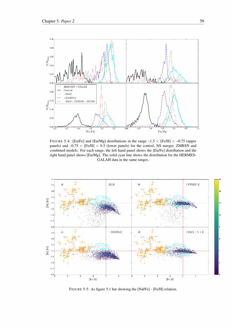
Chapter 5. Paper 2 59
FIGURE 5.4: [Eu/Fe] and [Eu/Mg] distributions in the range –1.5 < [Fe/H] < –0.75 (upperpanels) and –0.75 < [Fe/H] < 0.5 (lower panels) for the control, NS merger, ZMRSN andcombined models. For each range, the left hand panel shows the [Eu/Fe] distribution and theright hand panel shows [Eu/Mg]. The solid cyan line shows the distribution for the HERMES-
GALAH data in the same ranges.
FIGURE 5.5: As figure 5.1 but showing the [Nd/Fe] - [Fe/H] relation.

Chapter 5. Paper 2 60
drops to 0.0003 at high metallicity. This does allow for additional processes to be included how-
ever; by combining this model with NS mergers we have an excellent fit with observation for
[Fe/H] < –1 and a reasonable fit for –1 < [Fe/H] < 0.5. We are unable to replicate entirely the
slight downward trend observed at [Fe/H] > –1, though we do see a shallow downward trend
in the NS merger model. Observational data for the evolution of [Eu/α] typically shows a flat
trend with increasing [Fe/H]. This can be seen in Figure 5.2 which shows the [Eu/Mg] – [Fe/H]
relation. Comparisons to alpha elements rather than Fe provide insight into the formation sites.
Whereas [X/Fe] is driven at high [Fe/H] by large Fe production from Type Ia SNe, Mg is pri-
marily produced in CCSNe so [Eu/Mg] should be driven down by CCSNe. Clearly this is not
the case for the observed flat [Eu/Mg] trend (although it still displays high scatter at [Fe/H] <
–1.5, consistent with a strong, rare Eu production site), suggesting that the Mg production oc-
curs at similar rates as Eu production, relative to solar [Eu/Mg]. This matches with MRSNe as a
rare subset of HNe, explaining both the flatness and scatter at low metallicity. In Figure 5.2 our
ZMRSN model shows a relatively flat trend at [Fe/H] < –1 but underpredicts [Eu/Mg] at solar
[Fe/H]. This is improved by the inclusion of NS mergers and ECSNe which provide excellent
agreement with observations for –4 < [Fe/H] < 0.5. Figure 5.3 shows the median [Eu/Fe] and
[Eu/Mg] (upper and lower panels respectively) binned in 0.14 [Fe/H] intervals. The cyan obser-
vational data takes the median for each bin across all data sources (as such HERMES-GALAH
will dominate in the range [Fe/H] > –1.5 due to volume of data). The observed [Eu/Fe] and
[Eu/Mg] trends are closely matched by the combined ZMRSN, NS merger and ECSNe model
in both cases. The ZMRSN model alone arguably provides a better fit to the trend but offset
by ∼ –0.5, and could possibly be a good fit with increased fMRSN. However, as fMRSN depends
directly on [Fe/H] for the ZMRSN model, the evolution of the [Eu/Fe] trend is not so simple and
more constraints on the fraction of stars with appropriate rotation and magnetic fields is prob-
ably required. In Figure 5.4 we compare the [Eu/Fe] and [Eu/Mg] abundance distributions for
narrow [Fe/H] slices within the HERMES-GALAH range. The upper panels show the [Eu/Fe]
and [Eu/Mg] (left and right respectively) distributions in the range –1.5 < [Fe/H] < –0.75 and
the lower panels show the [Eu/Fe] and [Eu/Mg] distributions in the range –0.75 < [Fe/H] < 0.5.
In the range –1.5 < [Fe/H] < -0.75 both the [Eu/Fe] and [Eu/Mg] distributions match the obser-
vations best with the combined model. The [Eu/Mg] peak is positioned at slightly lower [Fe/H]
and is rather less spread out than observed, however this spread may be increased in reality by
metal mixing. Similarly, both [Eu/Fe] and [Eu/Mg] are good matches in the –0.75 < [Fe/H] <
0.5 range with the [Eu/Fe] peak showing slightly less scatter than expected.
Figure 5.5 shows the [Nd/Fe] – [Fe/H] relation, with panel layout as in Figure 5.1. Nd is ex-
pected to be produced in both s-process and r-process sites; this can be seen in panel a) which
shows a closer match to observations with the inclusion of AGB yields as the main s-process
site. The inclusion of NS mergers gives a good match to observational data at solar [Nd/Fe]
and [Fe/H], however a large scatter still exists at –2 < [Fe/H] < 0 as NS mergers are unable to

Chapter 5. Paper 2 61
FIGURE 5.6: Abundance relation for [Dy/Fe] (upper panel) and [Yb/Fe] (lower panel) for –4< [Fe/H] < –1. The orange data points are from Roederer et al. (2014), which was the only ofour four data sets with measurements for Dy and Yb. The green points show our simulated star
particles.
produce Nd quickly enough to raise [Nd/Fe]. The ZMRSN model matches the trend quite well
but [Nd/Fe] is consistently offset below observations by ∼ 0.5. The combined model provides
the best fit at [Fe/H] > –2. It also reproduces the large scatter at [Fe/H] < –2 for [Nd/Fe] > 0,
however it does not match the observed scatter as well at [Nd/Fe] < 0. Additionally in Figure
5.6 we show low metallicity end of the abundance patterns for both [Dy/Fe] and [Yb/Fe]. Dy
is an almost entirely r-process element and Yb can be formed by both the s-process and the
r-process, similar to Nd. The upper panel shows [Dy/Fe] for the combined model and the low
panel shows [Yb/Fe] both in range –4 < [Fe/H] < –1. Both show a good match in trend and
scatter with the observational data.
5.3.2 s-process - Zr, Ba
Zr is a light s-process element and so expected to be produced by both the main and weak s-
processes in AGB stars and in the He burning shells of massive stars, with a small contribution
from the r-process. We show the [Zr/Fe] - [Fe/H] relation in Figure 5.7. Compared to the heavier
elements Zr has a higher [Zr/Fe] values (∼ –0.25) at solar [Fe/H] in the control model due to
Zr production in AGB stars. As with the previous abundances we have examined this model
results in a high scatter in the range –2 < [Fe/H] < 0 which is inconsistent with observations.
The inclusion of NS mergers increases the values of [Zr/Fe] slightly to solar values at [Fe/H]
∼ 0 but does not remove the large scatter. Conversely, the inclusion of ZMRSN removes the

Chapter 5. Paper 2 62
FIGURE 5.7: As figure 5.1 but showing the [Zr/Fe] - [Fe/H] relation.
FIGURE 5.8: As figure 5.1 but showing the [Ba/Fe] - [Fe/H] relation.
Chapter 5. Paper 2 63
scatter but leaves [Zr/Fe] < 0, suggesting that the scatter is built up from relatively early AGB
enrichment. The combined model with both additions (also ECSNe which we expect to make
reasonable contributions up to the second s-process peak) matches observations very well for
[Fe/H] < 0, but overpredicts [Zr/Fe] at higher [Fe/H] where we should see a downward rather
than flat trend.
Finally in Figure 5.8 we show the [Ba/Fe] – [Fe/H] relation. As a heavy s-process element
we expect Ba to be produced largely by AGB stars. The control model shows [Ba/Fe] levels
of ∼ –0.25 at [Fe/H] = 0, slightly below observed levels. It also shows a large scatter below
[Ba/Fe] = –0.5 in the –2 < [Fe/H] < 0 range which is inconsistent with observations; neither
does it reproduce the observed trend at [Fe/H] < –2. Unsurprisingly, the addition of NS mergers
or ZMRSN does not change the simulated data significantly, either independently or together
with ECSNe. The addition of ZMRSN does have a small effect on the anomalous scatter at
–2 < [Fe/H] < 0; as ZMRSN are primarily operating at low [Fe/H] this suggests that altering
this feature requires changes at low [Fe/H]. Overall, our [Ba/Fe] abundance patterns are a poor
match with observations.
5.4 Discussion
In the previous section we showed two results which we discuss further here. We show that
our ZMRSN model is able to reproduce excellently abundance patterns for Eu, Nd, Dy and Yb
for [Fe/H] < 0. The fit is better when NS mergers are also included, contributing at higher
[Fe/H], but the overall fit with just NS mergers is poor. However, there is no direct observational
evidence for MRSNe, a fact which is compounded by the notion that they are less likely to occur
in present day galaxies with higher [Fe/H]. The question that therefore remains: is it possible
to reproduce the observed trends by modifying NS merger models? Part of this question hinges
on the uncertainty in the NS merger rate - better constraints on this will help to determine
if additional processes are required and how much they should contribute to the galactic r-
process. Nonetheless DTD models can be used to estimate NS merger rates and combined with
nucleosynthesis yields can constrain required rates to explain abundance patterns. A common
problem is the difficulty in explaining the decreasing [r-process/Fe] trend at high metallicity
using the expected t−1 DTD, which gives a trend much flatter than expected. Beniamini and
Piran (2019) showed that in one zone calculations, assuming no delay between formation and
merging of binary systems could reproduce this downward trend in [Eu/Fe], however it did not
appear to explain the scatter at [Fe/H] < –1. The minimum delay time adopted for the DTD
model seems to have a large impact on the [Eu/Fe] trend even at [Fe/H] > –1.5 (see Appendix
A of Cote et al. 2018), with shorter delay times resulting in greater [Eu/Fe] enrichment at low
[Fe/H]. The DTD we use (Mennekens and Vanbeveren, 2014) has a low minimum delay (∼

Chapter 5. Paper 2 64
10 Myr) and a further reduction is unlikely to reproduce the solar [Fe/H] downward trend or
increase [Eu/Fe] at [Fe/H] < –1. In order to reproduce the downward trend either a) a steeper
DTD must be adopted or b) strong Eu production must take place at low [Fe/H] with a stronger
downward trend than NS mergers across the same [Fe/H] range. Given that our choice for
fMRSN drops to almost zero for Z > 0.02 and gives a good match to observations across a range
of r-process elements for low Z stars it seems likely that a steeper DTD is required.
Additionally, we find that our SFR is too high at late times. This may contribute slightly to the
excess of metal produced however as noted in HK19 we find that our [α/Fe] - [Fe/H] relation is
a good match with observations and that the overly high SFR late at late times likely only results
in the formation of some very super-solar metallicity stars. Nonetheless, in a future work we
intend to examine the effect of using various SNe feedback models to supress SFR on chemical
enrichment.
In Figure 5.8 we showed the [Ba/Fe] – [Fe/H] relation. The observed increasing trend of [Ba/Fe]
from [Fe/H] ∼ –3 suggests that Ba production needs to start post Fe enrichment from early
CCSNe. AGB stars fit this model, but the increase is shifted to higher [Fe/H], so the AGB
contribution comes too late. Given the long lived nature of the low mass stars (M < 3 M)
required, it is difficult to shift the onset of Ba production to earlier times. One possible solution
is in the cores of massive stars which typically can only produce a weak s-process. However,
recently it has been suggested that mixing induced by sufficiently rapid rotation in these stars
can provide additional neutron sources, particularly at low metallicity, resulting in an increase
in s-process production and shift to heavier s-process elements (Chiappini et al., 2011; Cescutti
et al., 2015; Frischknecht et al., 2016). Inclusion of yields from these spin stars could provide
additional Ba at low [Fe/H] and could better reproduce observations.
5.5 Conclusions
In section 5.3 we presented the abundance relations for Eu, Nd, Dy, Yb, Zr and Ba for four
model galaxies including a number of r-process sites. In particular we present a combined
model of NS mergers, Z-dependent MRSNe and ECSNe as our best match to observational
data. In section 5.4 we provided some additional discussion. Figures 5.1, 5.5 and 5.6 showed
that [Eu/Fe], [Nd/Fe], [Dy/Fe] and [Yb/Fe] are an excellent match in both average abundance
and scatter in the –3 < [Fe/H] < –1 range. Between –1 < [Fe/H] < 0 the observational data
suggests a downward trend for [Eu/Fe] (HERMES-GALAH and Zhao et al. 2016) and to a lesser
extent [Nd/Fe]. The combined model shows a slightly flatter trend than this suggesting that our
model is overproducing europium in high [Fe/H] stars. We suggest that this could be remedied
by the choice of DTD for NS mergers, something which requires further study. We propose that
only a combined model of Z-dependent MRSNe and NS mergers is able to explain both the low

Chapter 5. Paper 2 65
[Fe/H], high scatter [r-process/Fe] trend and the decreasing trend at solar [Fe/H]. We also found
that the [Ba/Fe] increase occurred at too high [Fe/H]. We suggest that this points to the inclusion
of an additional s-process in rapidly rotating massive stars in the early universe.
Chapter 6
The Effects of Feedback Model onChemical Enrichment
In this chapter I will discuss the effects of feedback model choice on chemical enrichment. This
forms the basis for a third paper, although more work is needed before it is ready for submission.
6.1 Introduction
Supernova feedback is a crucial mechanism in the evolution of galaxies. The deaths of stars
release large quantities of metals and energy into their surroundings influencing the formation of
the next stars. In particular energy feedback from supernovae (SNe) is an important mechanism
in preventing excessive star formation by injecting heat and momentum into the surrounding
gas. Additionally SNe feedback can drive outflows of metal enriched gas into the intergalactic
medium (IGM).
Historically cosmological and numerical simulations have resulted in star formation rates (SFRs)
somewhat in excess of observations and have had difficulty in suppressing this. This difficulty
arises due to the fact that simulations often have mass resolutions in excess of thousands of solar
masses and as such are unable to resolve supernova remnants. The simple case of distributing
the energy from a SN event into the ISM as heat proves ineffective as the energy is free to be
radiated away with little effect on star formation.
Various models have tried to rectify this issue. Some models simply turn off cooling in the
affected gas particles for a short time (see Stinson et al. 2006, Teyssier et al. 2013) to maintain
the heating effect, thereby preventing star formation and driving thermal outflow. Dalla Vecchia
and Schaye (2012) used a stochastic approach where larger amounts of energy are assigned to
fewer gas particle (see Crain et al. 2015 for application in the EAGLE simulations). The stronger
66

Chapter 6. Paper 3 67
heating of particles allows SFR suppression prior to cooling occuring. Kinetic models (such as
Dalla Vecchia and Schaye 2008, Navarro and White 1993) assign a fraction of the SN energy
to be distributed as a velocity kick instead of as thermal energy in order to reduce gas density
required for star formation. It should be noted here that Kobayashi (2005) found that a similar
model of kinetic feedback gave metallicity gradients that too shallow to match observations as a
result of metal rich gases being driven from the core. Similar mechanical models distribute some
energy as momentum and additionally try to account for any unresolved Sedov-Taylor phase of
SNe expansion (Hopkins et al., 2014).
In this paper we examine the effect of four different feedback models: the standard thermal
model, a kinetic fraction model, a version of the stochastic model as in Dalla Vecchia and Schaye
(2012) and a version of the mechanical model as in Hopkins et al. (2014).
6.2 Models and Parameters
The code used is the same as in the previous works Kobayashi et al. (2007a) and chapters 4
and 5 and includes the same physical processes (radiative cooling, UVB heating, star formation,
etc.). The hydrodynamics is based on the SPH code GADGET-3 (see Springel 2005 for the
similar GADGET-2). The chemical enrichment for type Ia and type II SNe, HNe, SW and the
contribution from AGB stars is the same as in Haynes and Kobayashi (2019) (note yields from
the r-process sites, NS mergers, MRSNe, ECSNe and neutrino winds, are not included). In
order to examine the effect on galactic wind we compare four feedback models. The thermal
model is the default feedback method and the same as used in the works above. The kinetic,
stochastic and mechanical models all introduce free parameters which will be discussed below
in the context of isolated dwarf galaxies. These simulations are much faster than Milky Way
simulations so provide good testing environments for both code and parameters.
6.2.1 Kinetic Feedback
Kinetic feedback uses a parameter fk that represents the fraction of energy from a SNe event
that is distributed as kinetic energy. It therefore sits somewhere between 0 and 1, with 0 being
indistinguishable from the thermal model and 1 having zero thermal energy distributed. The
kinetic energy fraction is converted to a velocity which is applied as a kick to the gas particle
directly away from the SNe event. The conversion of thermal energy takes place after the energy
weighting due to the smoothing kernel is calculated. As one of the primary drivers of non
thermal feedback is to prevent excessive star formation, Figure 6.1 shows the SFR for three
different kinetic parameters: 0.01, 0.05 and 0.1 (dashed lines), in addition to the default thermal
model (solid black line). For fk = 0.01, the model closely matches the thermal model. Beyond

Chapter 6. Paper 3 68
FIGURE 6.1: The SFR in isolated dwarf galaxies for the thermal model (solid black line) andthree kinetic parameters (dashed lines).
that a clear trend is visible; increasing fk decreases SFR. Note that increasing it beyond ∼ 0.25
causes some problems with simulation runs not completing. This has been a recurring problem
with kinetic feedback when using high values for fk and may be related to gas particles becomes
spread over too large an area. Prior to this value it is possible for kinetic feedback to dismantle
the gas disc entirely. We found fk = 0.1 to be optimal for isolated dwarf galaxies.
6.2.2 Stochastic Feedback
The stochastic feedback model is based on the feedback model presented in Dalla Vecchia and
Schaye (2012). As in Dalla Vecchia and Schaye (2012) we define an energy increase, ∆e, which
is used to heat the neighbour particles around the SNe event. We choose
∆e = fESN
Nngb, (6.1)
where ESN is the SNe energy from the star particle during a given timestep and Nngb is the
number of feedback neighbour particles. At the point of feedback, a random number is generated
for each of the neighbour particles and compared to
r <ESNM∗
∆e ∑Nngbi Mi
, (6.2)

Chapter 6. Paper 3 69
FIGURE 6.2: The SFR in isolated dwarf galaxies for the thermal model (solid black line) andfive stochastic parameters (dashed lines).
where M∗ is the mass of the star particle. We note that our value of ∆e scales with the available
SNe energy for a given timestep. The parameter we introduce, f , is simply a scaling factor for
the approximate minimum energy for the probability function to hold,
∆e >ESN
Nngb, (6.3)
which gives a probability of 1 (i.e. each particle will receive an energy increase of ∆e). Substi-
tuting f = ESN / Nngb into the probability function gives the probability of any given particle
receiving an energy increase, which will scale as the reciprocal of f and give the expected num-
ber of particles that receive the energy
NFB =Nngb
f. (6.4)
Given the choice of Nngb = 36 ± 2, we choose values of f = 12, 18, 24, and 36. The results of
these simulations are shown in Figure 6.2 as dotted lines and again compared with thermal (solid
black line). Using f = 24 gave a SFR very similar to the thermal model. The lower parameter
choices (12 and 18) resulted in higher SFRs. Using f = 36 results in each SNe event heating
on average one gas particle and gave a suppressed SFR. We want to avoid using f > NNGB as it
resulted in an expectation value of less than 1 (although it is still possible that no particles are
heated even with lower values of f ) and additionally represents a greater increase in energy than
the SNe event can produce (although this is again possible for any given SNe event and choice

Chapter 6. Paper 3 70
FIGURE 6.3: The SFR in isolated dwarf galaxies for the thermal model (solid black line) andthree mechanical parameters (dot-dashed lines).
of f , if f > NNGB then any energy feedback that occurs will violate this). Additionally, feedback
to a single particle corresponds to the fiducial energy increase used in Dalla Vecchia and Schaye
(2012).
6.2.3 Mechanical Feedback
Mechanical feedback is based on the work in Hopkins et al. (2014) and Smith et al. (2018) and
attempts to take into account the work done by the SNe shock wave during the Sedov-Taylor
phase of expansion. Similar to the kinetic model a fraction of SNe energy, fk, is converted to a
momentum kick. As in Smith et al. (2018) the momentum is boosted by
∆P = ∆P0×
√1+
Mi
MejWi, (6.5)
where ∆P0 is the momentum initially input into the gas, Mi is the mass of the ith particle and
MejWi is mass received by the ith particle. This is limited by the total momentum at the point
where the shock wave exits the Sedov-Taylor phase,
∆P = ∆P0×3×1010(
ZZ
)−0.14 E16/17SN n−2/17
H√2MejESN1051
ergs cm s−1M, (6.6)
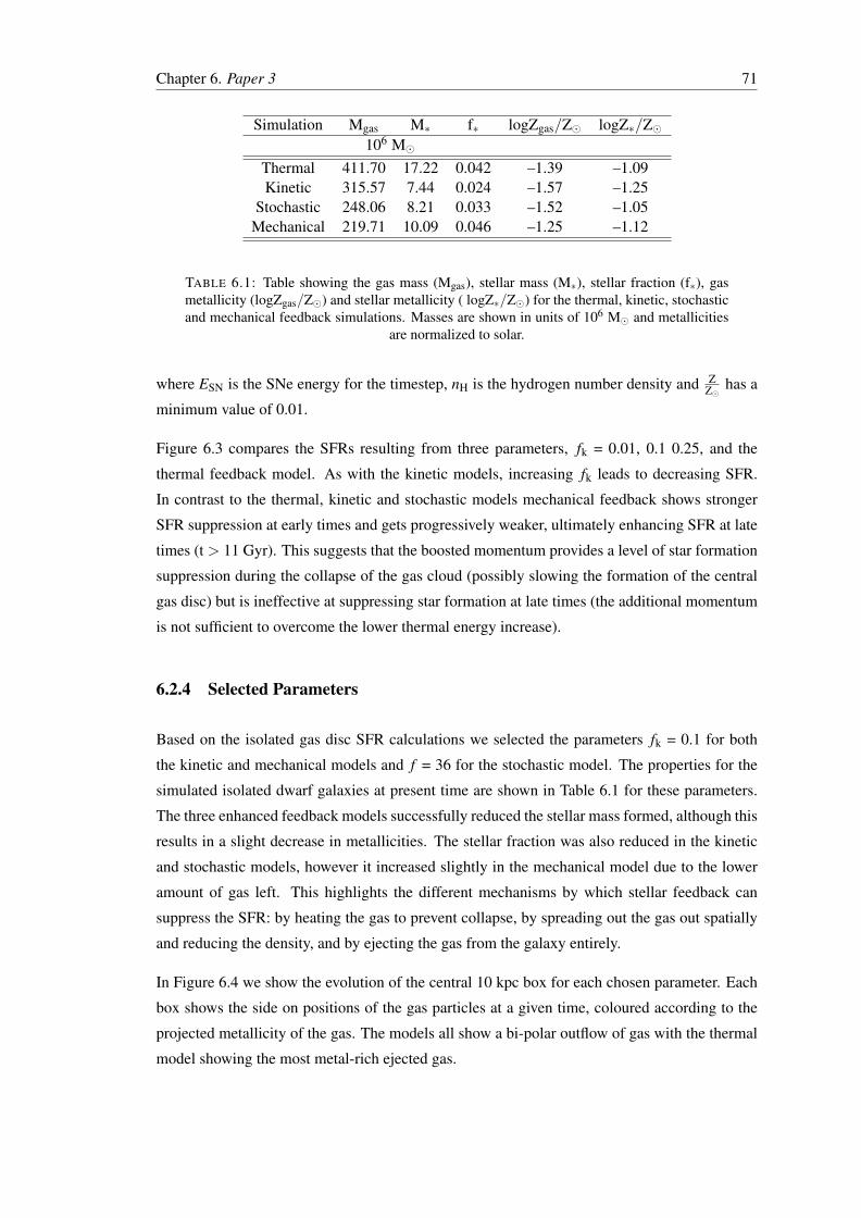
Chapter 6. Paper 3 71
Simulation Mgas M∗ f∗ logZgas/Z logZ∗/Z106 M
Thermal 411.70 17.22 0.042 –1.39 –1.09Kinetic 315.57 7.44 0.024 –1.57 –1.25
Stochastic 248.06 8.21 0.033 –1.52 –1.05Mechanical 219.71 10.09 0.046 –1.25 –1.12
TABLE 6.1: Table showing the gas mass (Mgas), stellar mass (M∗), stellar fraction (f∗), gasmetallicity (logZgas/Z) and stellar metallicity ( logZ∗/Z) for the thermal, kinetic, stochasticand mechanical feedback simulations. Masses are shown in units of 106 M and metallicities
are normalized to solar.
where ESN is the SNe energy for the timestep, nH is the hydrogen number density and ZZ
has a
minimum value of 0.01.
Figure 6.3 compares the SFRs resulting from three parameters, fk = 0.01, 0.1 0.25, and the
thermal feedback model. As with the kinetic models, increasing fk leads to decreasing SFR.
In contrast to the thermal, kinetic and stochastic models mechanical feedback shows stronger
SFR suppression at early times and gets progressively weaker, ultimately enhancing SFR at late
times (t > 11 Gyr). This suggests that the boosted momentum provides a level of star formation
suppression during the collapse of the gas cloud (possibly slowing the formation of the central
gas disc) but is ineffective at suppressing star formation at late times (the additional momentum
is not sufficient to overcome the lower thermal energy increase).
6.2.4 Selected Parameters
Based on the isolated gas disc SFR calculations we selected the parameters fk = 0.1 for both
the kinetic and mechanical models and f = 36 for the stochastic model. The properties for the
simulated isolated dwarf galaxies at present time are shown in Table 6.1 for these parameters.
The three enhanced feedback models successfully reduced the stellar mass formed, although this
results in a slight decrease in metallicities. The stellar fraction was also reduced in the kinetic
and stochastic models, however it increased slightly in the mechanical model due to the lower
amount of gas left. This highlights the different mechanisms by which stellar feedback can
suppress the SFR: by heating the gas to prevent collapse, by spreading out the gas out spatially
and reducing the density, and by ejecting the gas from the galaxy entirely.
In Figure 6.4 we show the evolution of the central 10 kpc box for each chosen parameter. Each
box shows the side on positions of the gas particles at a given time, coloured according to the
projected metallicity of the gas. The models all show a bi-polar outflow of gas with the thermal
model showing the most metal-rich ejected gas.
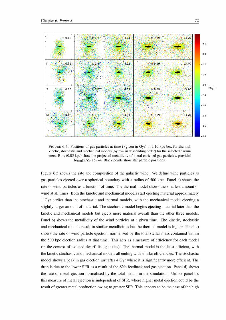
Chapter 6. Paper 3 72
FIGURE 6.4: Positions of gas particles at time t (given in Gyr) in a 10 kpc box for thermal,kinetic, stochastic and mechanical models (by row in descending order) for the selected param-eters. Bins (0.05 kpc) show the projected metallicity of metal enriched gas particles, provided
log10(Z/Z) > –4. Black points show star particle positions.
Figure 6.5 shows the rate and composition of the galactic wind. We define wind particles as
gas particles ejected over a spherical boundary with a radius of 500 kpc. Panel a) shows the
rate of wind particles as a function of time. The thermal model shows the smallest amount of
wind at all times. Both the kinetic and mechanical models start ejecting material approximately
1 Gyr earlier than the stochastic and thermal models, with the mechanical model ejecting a
slightly larger amount of material. The stochastic model begins ejecting material later than the
kinetic and mechanical models but ejects more material overall than the other three models.
Panel b) shows the metallicity of the wind particles at a given time. The kinetic, stochastic
and mechanical models result in similar metallicities but the thermal model is higher. Panel c)
shows the rate of wind particle ejection, normalised by the total stellar mass contained within
the 500 kpc ejection radius at that time. This acts as a measure of efficiency for each model
(in the context of isolated dwarf disc galaxies). The thermal model is the least efficient, with
the kinetic stochastic and mechanical models all ending with similar efficiencies. The stochastic
model shows a peak in gas ejection just after 4 Gyr where it is significantly more efficient. The
drop is due to the lower SFR as a result of the SNe feedback and gas ejection. Panel d) shows
the rate of metal ejection normalised by the total metals in the simulation. Unlike panel b),
this measure of metal ejection is independent of SFR, where higher metal ejection could be the
result of greater metal production owing to greater SFR. This appears to be the case of the high

Chapter 6. Paper 3 73
FIGURE 6.5: Plots showing the effect of feedback model on galactic wind for the thermal,kinetic, stochastic and mechanical models with selected parameters. Ejected particles are thosethat move over a 500 kpc spherical boundary. Panel a) shows the rate of ejected gas particles.Panel b) shows the metallicity of the newly ejected gas at each timestep normalised to solarmetallicity. Panel c) shows the rate of ejected gas normalised by the stellar mass containedwithin the ejection radius. Panel d) shows the rate of ejected metals normalised by the total
mass of metals.
metallicity of ejected gas seen in the thermal model; in this panel all models consistently eject a
similar fraction of the total metals, with the exception of the stochastic ejection peak at 4 Gyr.
Additionally in Figure 6.6 we show the same panels as in Figure 6.5 but for the parameter
tests for the stochastic model (using f = 12, 18, 24, and 36, along with the thermal model).
Interestingly we found that using f = 18 resulted in a reasonable match with the thermal model
in all four panels. Increasing f resulted in stronger wind (corresponding with decreased SFR),
greater ejection efficiency and a larger fraction of metals ejected. This suggests that it is possible
to have similar metal ejection as in the thermal model, though without the decreased SFR from
the f = 36 model.
6.3 Milky Way Galaxies
In this section we use the selected parameters from the isolated dwarf disc galaxies to simulate
Milky Way-type galaxies. We use initial conditions from Scannapieco et al. (2012) with cos-
mological parameters: H0 = 100h = 73 km s−1 Mpc−1, Ω0 = 0.25, ΩΛ = 0.75, ΩB = 0.04 with

Chapter 6. Paper 3 74
FIGURE 6.6: As Figure 6.5 but comparing stochastic feedback models with differing values off .
a gravitational softening length of 1 kpc h−1 and initial gas particle mass of 3.5×10⁶M. Two
problems occurred with these simulations. The first was partially computational; the chosen pa-
rameter for the kinetic model proved far too strong and would entirely dismantle the gas disc by
z=1. This in turn led to extremely long computational times, likely as a result of the unexpected
number of particles at large distances. Reducing the parameter, eventually down to fk, we found
that the feedback was still far too strong and the runtime far too time consuming. Additionally,
we found that the selected parameters for both the stochastic and mechanical models did not
suppress the SFR as they had done in the isolated dwarf disc galaxies. Unfortunately, this sug-
gests that the optimal parameters for isolated dwarf disc galaxies do not translate to the optimal
parameters for Milky Way-type galaxies. In order to determine these we would require a param-
eter study using Milky Way-type galaxies. Nonetheless, we present the simulations completed
thus far in this section, using the chosen parameters.
Table 6.2 shows the galactic properties for the simulated galaxies. We adopt the selected param-
eters from the previous section for the stochastic and mechanical models ( f = 36 and fk = 0.1
respectively). An effective solar neighbourhood is defined as in Chapter 4 and values are given
for both the central 10 kpc disc with height± 2 kpc and the solar neighbourhood. Unexpectedly,
the thermal model shows the lowest stellar mass and stellar fraction in both cases. This can also
be seen in Figure 6.8, where we show the SFRs for both the central disc (dashed lines) and the

Chapter 6. Paper 3 75
10 kpc disc Solar NeighbourhoodSimulation Mgas M∗ f∗ SFR Effective SN Mgas M∗ f∗ SFR
109 M M y−1 kpc 109 M M y−1
Thermal 10.54 97.17 0.90 40.12 5.571 - 7.285 1.60 4.00 0.71 4.30Stochastic 10.04 113.37 0.92 85.41 5.850 - 7.650 1.22 4.72 0.79 2.43
Mechanical 10.26 104.31 0.91 37.17 5.083 - 6.647 1.46 6.38 0.81 4.78
TABLE 6.2: Properties for the simulated galaxies at z= 0 for the central 10 kpc disc with height± 2 kpc and the effective solar neighbourhood. All masses are given in terms of 109 M and
SFR is given in M y−1.
FIGURE 6.7: Positions of gas particles at redshift z within a 50 kpc box. Bins show theprojected metallicity of gas particles with Z/Z > –4.
effective solar neighbourhood (solid lines). The stochastic and mechanical models both have
higher SFRs than the thermal model, rather than supressing them.
One possible explanation for this is that the parameters adopted from the simpler isolated gas
discs do not result in effective SFR rate suppression. Figure 6.2 shows that too low a choice
of f results in stronger star formation than the thermal model in the isolated discs, suggesting
that a higher parameter for the stochastic model may result in a lower SFR here. It is also worth
noting that for the stochastic model, the change in the number of neighbour particles between
the isolated gas discs and Milky Way-type simulations, from 36 to 64 respectively, should have
had an effect. As the optimal choice of parameter appears to be approximately f = NNGB this
also suggests that a high choice of f could reduce the SFR.
In Figure 6.9 we show the simulated galactic wind ejected over a radius of 1 Gpc. The panel

Chapter 6. Paper 3 76
FIGURE 6.8: The SFR for the central 10 kpc disc with height ± 2 (dashed lines) and the solarneighbourhood (solid lines) for the thermal, stochastic and mechanical models.
layout is the same as used in Figure 6.5. Both the choice of feedback model and model param-
eter had a large impact on the galactic wind from the isolated dwarf disc galaxies. In particular,
the ejection efficiency of the non-thermal models was significantly higher and resulted in greater
mass ejection, even with lower SFR. However, the three Milky Way models show very little dif-
ference in wind rate, ejection efficiency of the metallicity of the ejected material. The stochastic
model has a slightly higher ejection efficiency than the other two models. This leads to a sec-
ond possible explanation for the lack of SFR suppression: that the steeper gravitational well is
preventing efficient gas ejection, and it was this process that was reducing star formation rate
within the isolated discs rather than gas heating.
To further examine this, we show the density-temperature phase space diagram in Figure 6.10.
This shows the temperature and density relation for each gas particle with a central spherical
volume with radius 1 Gpc in addition to showing the average distance from the centre for each
bin. Each part of this figure shows a different region of the simulated galaxy. The central gas disc
is comprised of the high density gas region, log10nH ' –1. The large low density gas reserve –7
' log10nH ' –4 shows gas outside the main gas disc supplemented by heated gas ejected from
the centre. The gas particles at log10nH ∼ 0 with elevated temperature are those heated by SNe
feedback. The problem with the stochastic model can be seen clearly in this region; although gas
particles are being heated (to a larger degree than the thermal and mechanical models), many
of the particles left at lower temperatures and higher densities are more likely to form stars.
A lower value of f would result in more star particles being heated, which might prevent the
cooling. The mechanical model appears similar to the thermal model, with a slightly greater

Chapter 6. Paper 3 77
FIGURE 6.9: As Figure 6.5 but for the thermal, stochastic and mechanical models for the MilkyWay-type galaxies, with an ejection radius of 1 Gpc.
number of high density particles. This is likely to be due to the slightly decreased thermal
component.
6.4 Conclusions and Future Work
In this Chapter we have presented a comparison of four SNe feedback models: thermal, kinetic,
stochastic and mechanical. Implementing them into models of isolated dwarf disc galaxies, we
tested a number of parameters for them and we found that the kinetic ( fk = 0.1), stochastic ( f
= 36) and mechanical ( fk = 0.1) models decreased the SFR as intended. We additionally found
that they did not proportionally eject more or less metals than the thermal model, however the
metal content of galactic wind did vary naturally as a result of the lower SFR.
We then attempted to implement the feedback models into simulations of Milky Way-type galax-
ies and encountered several problems:
• Due to the increased mass, the kinetic feedback model becomes too efficient at ejecting
material and would completely dismantle the gas disc.
• The stochastic and mechanical models adopting the parameters from the isolated gas disc
models were showing an increased SFR, contrary to what was expected.

Chapter 6. Paper 3 78
FIGURE 6.10: Density-temperature phase space diagram for the central sphere of radius 1 Gpcfor the thermal, stochastic and mechanical models (T, S and M respectively). nH is the hydrogen
number density and the colour denotes distance in Gpc from the centre of the galactic disc.
One method to resolve these problems would be to determine parameters using Milky Way
simulations for the kinetic, stochastic and mechanical models. In particular the stochastic model
parameter affects both the energy a particle receives and how many particles are expected to
receive it. This would be very time consuming however.
Chapter 7
Summary
In this Chapter I will present a brief summary of the work contained in this thesis.
In Chapter 2 I presented the theory and background behind the nucleosynthesis processes that
could contribute to the creation of elements heavier than iron. Of these processes, the slow and
rapid neutron capture processes were best able to explain the chemical abundances we observe
today. I further examined some of the potential sites where the conditions for these processes
were able to occur:
• A strong s-process in the thermal pulses of low mass AGB stars via the 13C neutron source.
• A weak s-process in high mass AGB stars via the 22Ne neutron source.
• A strong r-process source in the dynamic and neutron-rich ejecta of merging neutron stars.
• A strong r-process source in the supernovae of highly magnetised and rapidly rotating
massive stars, ejected by polar jets.
• A weak r-process source in electron capture supernovae.
• A weak r-process source in the neutrino driven winds of supernovae.
I presented in Chapter 3 an overview of the chemodynamical code used in the simulations, in-
cluding the hydrodynamics, star formation process, chemical enrichment, supernova yields and
supernova feedback. I then discussed the implementation of the processes I examined in Chapter
2 into the code. Yields were adopted for AGB stars and included in the chemical enrichment.
For neutron star mergers, yields and a delay time distribution for formation and coalescence
of binary neutron stars were adopted and combined to simulate the dynamic ejecta. Magneto-
rotational supernova yields were adopted and used to replace a fraction of high mass supernovae
events with an adjustable parameter. Electron capture supernova yields were included with a
79

Chapter 7. Summary 80
metallicity dependent mass range and neutrino driven wind yields were added for stars with
M > 13M. I also present here the implementation of several alternative supernova feedback
models in addition to the thermal and kinetic models already available: a stochastic model de-
signed to heat a smaller number of particles by a fixed energy and a mechanical model designed
to take into account the work done during the Sedov Taylor phase of supernova expansion.
In Chapter 4 I presented my first paper, previously accepted and published in Monthly Notices of
the Royal Astronomical Society, largely unchanged. In it I presented chemodynamical simula-
tions comparing NS mergers, MRSNe, ECSNe and neutrino winds in the context of both isolated
dwarf disc galaxies and Milky Way-type galaxies. Using analysis of the [Eu/(Fe,α)] - [Fe/H]
relations I concluded that, although NS mergers likely contribute to the galactic r-process, they
are unable to explain early, low [Fe/H] r-process enrichment and that an additional r-process
site, such as MRSNe, would be required to match observations.
In Chapter 5 I presented my second paper, largely ready for submission, that further examined
the role of MRSNe as a the driver of early galactic r-process enrichment. In particular, I adopted
the Z-dependency of hypernovae and applied this to the MRSNe model on the basis that the
rotation condition for MRSNe would be hampered by angular momentum loss due to increased
metallicity. I compared this ZMRSNe model with NS merger models for Chapter 4 and pre-
sented a combined ECSNe, NS mergers and ZMRSNe model that was able to reproduce low
metallicity observations for Eu, Nd, Dy, Er and Zr very well and this provided an improvement
on my previous paper.
In Chapter 6 I presented final paper comparing the thermal and kinetic feedback models to the
stochastic and mechanical feedback models. I found that the models worked well in the param-
eter study using isolated dwarf disc galaxies, and were able to suppress SFR when compared to
the thermal model. Although it appears that the metallicity of the galactic wind was increase
in the thermal model, it appears that this is due to the higher SFR. The chosen parameters did
not translate well to the Milky Way-type galaxies, although feedback appears to be inefficient in
MW type galaxies. This will require further study of the parameters for MW type galaxies.
7.0.1 Key Conclusions
The primary conclusions drawn from this work are listed below:
• MRSNe are shown to play an important role in the early r-process (traced by europium,
dysprosium, neodymium and ytterbium) enrichment of Milky Way type galaxies. In the
case of europium enrichment, this holds for both [Eu/Fe] and [Eu/α].
• NS mergers alone are unable to account for r-process enrichment in the early Milky Way,
despite being able to produce stars with solar [Eu/Fe] abundances at solar [Fe/H].

Chapter 7. Summary 81
• MRSNe with an metallicity dependence adopted from studies of HNe and combined with
NS mergers are able to accurately reproduce r-process trends.
7.0.2 Future Work
Finally here I list future work I would like to undertake myself and other future work that would
be beneficial to galactic archaeology:
• Higher resolution runs of the combined NS merger and ZMRSNe model presented in
Chapter 5. The simulation code includes inital conditions at two higher resolutions, so
the primary limiting factor is the long run times required (a rough estimation of at least
six months for the lower of the higher resolutions). This would allow me to better discuss
any resolution dependence and provide a much larger sample of low [Fe/H] star particles
for comparison to observations.
• In Chapter 5 I found that the simulated [Ba/Fe] matched poorly with the observed trend,
particularly at low [Fe/H]. In order to address this I would like to run simulations com-
paring the effects of the new AGB yields on s-process production. Additionally, updated
yields from rapidly rotating stars may have increased s-process production (disucssed in
Chapter 5); I would like to modify the code to include these in a similar way to MRSNe
(including these in conjunction with MRSNe may prove challenging as both have similar
progenitor stars).
• I would like to compare the effects of NS merger DTDs and the effect the choice has on
[Eu/Fe] – [Fe/H]. In particular, I would be interested to see the effect DTD choice could
have on the slope gradient at solar [Fe/H]. It currently appears unlikely that DTD choice
could enable NS mergers to explain r-process abundance patterns alone, however a study
into DTD choice would still prove valuable.
• The Milky Way feedback parameter testing discussed in Chapter 6. The parameter se-
lection based on the isolated dwarf disc galaxies did not produce the same effects when
transferred to the Milky Way type galaxies; a study of these parameters using Milky Way
type galaxies may result in an improved feedback model. In particular I would interested
to see the effects on r-process nucleosynthesis.
Bibliography
Abbott, B.P., Abbott, R., Abbott, T.D., et al., 2017a. Gravitational Waves and Gamma-Rays
from a Binary Neutron Star Merger: GW170817 and GRB 170817A. ApJ, 848:L13.
Abbott, B.P., Abbott, R., Abbott, T.D., et al., 2017b. GW170817: Observation of Gravitational
Waves from a Binary Neutron Star Inspiral. Physical Review Letters, 119(16):161101.
Anders, E. and Grevesse, N., 1989. Abundances of the elements - Meteoritic and solar. Geochim-
ica et Cosmochimica Acta, 53:197.
Arcones, A., Janka, H.T., and Scheck, L., 2007. Nucleosynthesis-relevant conditions in
neutrino-driven supernova outflows. I. Spherically symmetric hydrodynamic simulations.
A&A, 467:1227.
Argast, D., Samland, M., Thielemann, F.K., et al., 2004. Neutron star mergers versus core-
collapse supernovae as dominant r-process sites in the early Galaxy. A&A, 416:997.
Arnould, M. and Goriely, S., 2003. The p-process of stellar nucleosynthesis: astrophysics and
nuclear physics status. Physics Reports, 384:1.
Beer, H. and Macklin, R.L., 1989. Measurement of the Rb-85 and Rb-87 capture cross sections
for s-process studies. ApJ, 339:962.
Beniamini, P., Hotokezaka, K., and Piran, T., 2016. Natal Kicks and Time Delays in Merging
Neutron Star Binaries: Implications for r-process Nucleosynthesis in Ultra-faint Dwarfs and
in the Milky Way. ApJ, 829:L13.
Beniamini, P. and Piran, T., 2019. The Gravitational waves merger time distribution of binary
neutron star systems. MNRAS, 487:4847.
Berger, M.J. Colella, P., 1989. Local adaptive mesh refinement for shock hydrodynamics. Jour-
nal of Computational Physics, 82:64.
Bisterzo, S., Gallino, R., Straniero, O., et al., 2011. The s-process in low-metallicity stars -
II. Interpretation of high-resolution spectroscopic observations with asymptotic giant branch
models. MNRAS, 418:284.
82

Bibliography 83
Buder, S., Asplund, M., Duong, L., et al., 2018. The GALAH Survey: Second Data Release.
MNRAS.
Burbidge, E.M., Burbidge, G.R., Fowler, W.A., et al., 1957. Synthesis of the Elements in Stars.
Reviews of Modern Physics, 29:547.
Cameron, A.G.W., 1957. NUCLEAR REACTIONS IN STARS AND NUCLEOGENESIS.
Astronomical Society of the Pacific, 69:201.
Cameron, A.G.W., 1960. New Neutron Sources of Possible Astrophysical Importance. aj,
65:485.
Cameron, A.G.W., 2001. Some Properties of r-Process Accretion Disks and Jets. ApJ, 562:456.
Cameron, A.G.W., 2003. Some Nucleosynthesis Effects Associated with r-Process Jets. ApJ,
587:327.
Cescutti, G., Romano, D., Matteucci, F., et al., 2015. The role of neutron star mergers in the
chemical evolution of the Galactic halo. A&A, 577:A139.
Chiappini, C., Frischknecht, U., Meynet, G., et al., 2011. Imprints of fast-rotating massive stars
in the Galactic Bulge. Nature, 472:454.
Cote, B., Eichler, M., Arcones, A., et al., 2018. Neutron Star Mergers Might not be the Only
Source of r-Process Elements in the Milky Way. ArXiv e-prints.
Cowan, J.J. and Rose, W.K., 1977. Production of C-14 and neutrons in red giants. Astrophysical
Journal, 212:149.
Crain, R.A., McCarthy, I.G., Schaye, J., et al., 2013. Enriching the hot circumgalactic medium.
MNRAS, 432:3005.
Crain, R.A., Schaye, J., Bower, R.G., et al., 2015. The EAGLE simulations of galaxy formation:
calibration of subgrid physics and model variations. MNRAS, 450:1937.
Dalla Vecchia, C. and Schaye, J., 2008. Simulating galactic outflows with kinetic supernova
feedback. MNRAS, 387:1431.
Dalla Vecchia, C. and Schaye, J., 2012. Simulating galactic outflows with thermal supernova
feedback. MNRAS, 426:140.
Doherty, C.L., Gil-Pons, P., Siess, L., et al., 2015. Super- and massive AGB stars - IV. Final
fates - initial-to-final mass relation. MNRAS, 446:2599.
Freiburghaus, C., Rembges, J.F., Rauscher, T., et al., 1999a. The Astrophysical r-Process:
A Comparison of Calculations following Adiabatic Expansion with Classical Calculations
Based on Neutron Densities and Temperatures. ApJ, 516:381.

Bibliography 84
Freiburghaus, C., Rosswog, S., and Thielemann, F.K., 1999b. R-Process in Neutron Star Merg-
ers. ApJ, 525:L121.
Frischknecht, U., Hirschi, R., Pignatari, M., et al., 2016. s-process production in rotating mas-
sive stars at solar and low metallicities. MNRAS, 456:1803.
Frohlich, C., Martınez-Pinedo, G., Liebendorfer, M., et al., 2006. Neutrino-Induced Nucleosyn-
thesis of A>64 Nuclei: The νp Process. Physical Review Letters, 96(14):142502.
Gallino, R., Arlandini, C., Busso, M., et al., 1998. Evolution and Nucleosynthesis in Low-Mass
Asymptotic Giant Branch Stars. II. Neutron Capture and the S-Process. ApJ, 497:388.
Gilroy, K.K., Sneden, C., Pilachowski, C.A., et al., 1988. Abundances of neutron capture ele-
ments in Population II stars. ApJ, 327:298.
Gingold, R.A. and Monaghan, J.J., 1977. Smoothed particle hydrodynamics - Theory and ap-
plication to non-spherical stars. MNRAS, 181:375.
Hansen, C.J., Nordstrom, B., Hansen, T.T., et al., 2016. Abundances of carbon-enhanced metal-
poor stars as constraints on their formation. A&A, 588:A37.
Hansen, T.T., Holmbeck, E.M., Beers, T.C., et al., 2018. The R-process Alliance: First Release
from the Southern Search for R-process-enhanced Stars in the Galactic Halo. ApJ, 858:92.
Haynes, C.J. and Kobayashi, C., 2019. Galactic simulations of r-process elemental abundances.
MNRAS, 483:5123.
Hernquist, L. and Katz, N., 1989. TREESPH - A unification of SPH with the hierarchical tree
method. ApJ, 70:419.
Honda, S., Aoki, W., Ishimaru, Y., et al., 2006. Neutron-Capture Elements in the Very Metal
Poor Star HD 122563. ApJ, 643:1180.
Hopkins, P.F., Keres, D., Onorbe, J., et al., 2014. Galaxies on FIRE (Feedback In Realistic
Environments): stellar feedback explains cosmologically inefficient star formation. MNRAS,
445:581.
Iben, Jr., I. and Renzini, A., 1982a. On the formation of carbon star characteristics and the
production of neutron-rich isotopes in asymptotic giant branch stars of small core mass. ApJ,
263:L23.
Iben, Jr., I. and Renzini, A., 1982b. The role of semiconvection in bringing carbon to the surface
of asymptotic giant branch stars of small core mass. ApJ, 259:L79.
Janka, H.T., 2012. Explosion Mechanisms of Core-Collapse Supernovae. Annual Review of
Nuclear and Particle Science, 62:407.

Bibliography 85
Ji, A.P., Frebel, A., Simon, J.D., et al., 2016. Complete Element Abundances of Nine Stars in
the r-process Galaxy Reticulum II. ApJ, 830:93.
Kappeler, F., Gallino, R., Bisterzo, S., et al., 2011. The s process: Nuclear physics, stellar
models, and observations. Reviews of Modern Physics, 83:157.
Karakas, A.I., 2010. Updated stellar yields from asymptotic giant branch models. MNRAS,
403:1413.
Karakas, A.I., Garcıa-Hernandez, D.A., and Lugaro, M., 2012. Heavy Element Nucleosynthesis
in the Brightest Galactic Asymptotic Giant Branch Stars. ApJ, 751:8.
Karakas, A.I. and Lugaro, M., 2016. Stellar Yields from Metal-rich Asymptotic Giant Branch
Models. ApJ, 825:26.
Katz, N., 1992. Dissipational galaxy formation. ii-effects of star formation. ApJ, 391:502.
Kobayashi, C., 2004. GRAPE-SPH chemodynamical simulation of elliptical galaxies - I. Evo-
lution of metallicity gradients. MNRAS, 347:740.
Kobayashi, C., 2005. GRAPE-SPH chemodynamical simulation of elliptical galaxies - II. Scal-
ing relations and the fundamental plane. MNRAS, 361:1216.
Kobayashi, C., Karakas, A.I., and Umeda, H., 2011. The evolution of isotope ratios in the Milky
Way Galaxy. MNRAS, 414:3231.
Kobayashi, C. and Nakasato, N., 2011. Chemodynamical Simulations of the Milky Way Galaxy.
ApJ, 729:16.
Kobayashi, C. and Nomoto, K., 2009. The Role of Type Ia Supernovae in Chemical Evolution.
I. Lifetime of Type Ia Supernovae and Metallicity Effect. ApJ, 707:1466.
Kobayashi, C., Nomoto, K., and Hachisu, I., 2015. Subclasses of Type Ia Supernovae as the
Origin of [α/Fe] Ratios in Dwarf Spheroidal Galaxies. ApJ, 804:L24.
Kobayashi, C., Springel, V., and White, S.D.M., 2007a. Simulations of Cosmic Chemical En-
richment. MNRAS, 376:1465.
Kobayashi, C., Springel, V., and White, S.D.M., 2007b. Simulations of Cosmic Chemical En-
richment. MNRAS, 376:1465.
Kodama, T. and Arimoto, N., 1997. Origin of the colour-magnitude relation of elliptical galax-
ies. A&A, 320:41.
Korobkin, O., Rosswog, S., Arcones, A., et al., 2012. On the astrophysical robustness of the
neutron star merger r-process. MNRAS, 426:1940.

Bibliography 86
Kroupa, P., 2001. On the variation of the initial mass function. MNRAS, 322:231.
Kroupa, P., 2008. The IMF of Simple and Composite Populations. In J.H. Knapen, T.J. Ma-
honey, and A. Vazdekis, editors, Pathways Through an Eclectic Universe, volume 390 of
Astronomical Society of the Pacific Conference Series, page 3.
Lattimer, J.M. and Schramm, D.N., 1974. Black-hole-neutron-star collisions. ApJ, 192:L145.
Lucy, L.B., 1977. A numerical approach to the testing of the fission hypothesis. AJ, 82:1013.
Lugaro, M., Ugalde, C., Karakas, A.I., et al., 2004. Reaction Rate Uncertainties and the Pro-
duction of 19F in Asymptotic Giant Branch Stars. ApJ, 615:934.
Mackereth, J.T., Crain, R.A., Schiavon, R.P., et al., 2018. The origin of diverse α-element
abundances in galaxy discs. MNRAS, 477:5072.
Maoz, D., Mannucci, F., and Nelemans, G., 2014. Observational Clues to the Progenitors of
Type Ia Supernovae. Annual Review of Astronomy and Astrophysics, 52:107.
Mennekens, N. and Vanbeveren, D., 2014. Massive double compact object mergers: gravita-
tional wave sources and r-process element production sites. A&A, 564:A134.
Merrill, P., 1952. Spectroscopic observations of stars of class Md. Astrophysics Journal, 116.
Metzger, B.D. and Fernandez, R., 2014. Red or blue? A potential kilonova imprint of the delay
until black hole formation following a neutron star merger. MNRAS, 441:3444.
Miyaji, S., Sugimoto, D., Nomoto, K., et al., 1980. Supernova explosion triggered by electron
capture and formation of a neutron star. International Cosmic Ray Conference, 2:13.
Mosta, P., Roberts, L.F., Halevi, G., et al., 2018. r-process Nucleosynthesis from Three-
dimensional Magnetorotational Core-collapse Supernovae. ApJ, 864:171.
Navarro, J.F. and White, S.D.M., 1993. Simulations of Dissipative Galaxy Formation in Hierar-
chically Clustering Universes - Part One - Tests of the Code. MNRAS, 265:271.
Nishimura, N., Takiwaki, T., and Thielemann, F.K., 2015. The r-process Nucleosynthesis in the
Various Jet-like Explosions of Magnetorotational Core-collapse Supernovae. ApJ, 810:109.
Nomoto, K., Iwamoto, K., Nakasato, N., et al., 1997. Nucleosynthesis in type Ia supernovae.
Nuclear Physics A, 621:467.
Ojima, T., Ishimaru, Y., Wanajo, S., et al., 2017. Stochastic Chemical Evolution of Sub-Halos
and the Origin of r-Process Elements. In S. Kubono, T. Kajino, S. Nishimura, T. Isobe,
S. Nagataki, T. Shima, and Y. Takeda, editors, 14th International Symposium on Nuclei in the
Cosmos (NIC2016), page 020208.

Bibliography 87
Ojima, T., Ishimaru, Y., Wanajo, S., et al., 2018. Stochastic Chemical Evolution of Galactic
Subhalos and the Origin of r-process Elements. ApJ, 865:87.
Prantzos, N., Hashimoto, M., and Nomoto, K., 1990. The s-process in massive stars - Yields as
a function of stellar mass and metallicity. A&A, 234:211.
Roederer, I.U., 2017. The Origin of the Heaviest Metals in Most Ultra-faint Dwarf Galaxies.
ApJ, 835:23.
Roederer, I.U., Cowan, J.J., Karakas, A.I., et al., 2010. The Ubiquity of the Rapid Neutron-
capture Process. ApJ, 724:975.
Roederer, I.U., Preston, G.W., Thompson, I.B., et al., 2014. A Search for Stars of Very Low
Metal Abundance. VI. Detailed Abundances of 313 Metal-poor Stars. aj, 147:136.
Ruffert, M., Janka, H.T., and Schaefer, G., 1996. Coalescing neutron stars - a step towards
physical models. I. Hydrodynamic evolution and gravitational-wave emission. A&A, 311:532.
Scannapieco, C., Wadepuhl, M., Parry, O.H., et al., 2012. The Aquila comparison project: the
effects of feedback and numerical methods on simulations of galaxy formation. MNRAS,
423:1726.
Shen, S., Cooke, R.J., Ramirez-Ruiz, E., et al., 2015. The History of R-Process Enrichment in
the Milky Way. ApJ, 807:115.
Shen, S., Wadsley, J., and Stinson, G., 2010. The enrichment of the intergalactic medium with
adiabatic feedback - I. Metal cooling and metal diffusion. MNRAS, 407:1581.
Shibata, M. and Uryu, K.o., 2000. Simulation of merging binary neutron stars in full general
relativity: Γ=2 case. Physical Review D, 61(6):064001.
Smith, M.C., Sijacki, D., and Shen, S., 2018. Supernova feedback in numerical simulations of
galaxy formation: separating physics from numerics. MNRAS, 478:302.
Smith, V.V. and Lambert, D.L., 1986. The chemical composition of red giants. II - Helium
burning and the s-process in the MS and S stars. ApJ, 311:843.
Smith, V.V. and Lambert, D.L., 1990. The chemical composition of red giants. III - Further
CNO isotopic and s-process abundances in thermally pulsing asymptotic giant branch stars.
ApJ, 72:387.
Sneden, C., Cowan, J.J., and Gallino, R., 2008. Neutron-Capture Elements in the Early Galaxy.
Annual Review of Astronomy and Astrophysics, 46:241.
Sneden, C. and Parthasarathy, M., 1983. The r- and s-process nuclei in the early history of the
galaxy - HD 122563. ApJ, 267:757.

Bibliography 88
Sneden, C., Preston, G.W., McWilliam, A., et al., 1994. Ultrametal-poor halo stars: The re-
markable spectrum of CS 22892-052. ApJ, 431:L27.
Springel, V., 2005. The cosmological simulation code GADGET-2. MNRAS, 364:1105.
Springel, V. and Hernquist, L., 2002. Cosmological smoothed particle hydrodynamics simula-
tions: the entropy equation. MNRAS, 333:649.
Springel, V. and Hernquist, L., 2003. Cosmological smoothed particle hydrodynamics simula-
tions: a hybrid multiphase model for star formation. MNRAS, 339:289.
Sterling, N.C. and Dinerstein, H.L., 2008. The Abundances of Light Neutron-Capture Elements
in Planetary Nebulae. II. s-Process Enrichments and Interpretation. ApJ, 174:158.
Stinson, G., Seth, A., Katz, N., et al., 2006. Star formation and feedback in smoothed particle
hydrodynamic simulations - I. Isolated galaxies. MNRAS, 373:1074.
Sutherland, R. and Dopita, M., 1993. Cooling functions for low-density astrophysical plasmas.
ApJ, 88:253 .
Tanaka, M., Utsumi, Y., Mazzali, P.A., et al., 2017. Kilonova from post-merger ejecta as an
optical and near-Infrared counterpart of GW170817. Publications of the Astronomical Society
of Japan, 69:102.
Taylor, P. and Kobayashi, C., 2014. Seeding black holes in cosmological simulations. MNRAS,
442:2751.
Teyssier, R., Pontzen, A., Dubois, Y., et al., 2013. Cusp-core transformations in dwarf galaxies:
observational predictions. MNRAS, 429:3068.
Tolstoy, E., Hill, V., and Tosi, M., 2009. Star-Formation Histories, Abundances, and Kinemat-
ics of Dwarf Galaxies in the Local Group. Annual Review of Astronomy and Astrophysics,
47:371.
Valenti, S., David, Sand, J., et al., 2017. The Discovery of the Electromagnetic Counterpart of
GW170817: Kilonova AT 2017gfo/DLT17ck. ApJ, 848:L24.
van Aarle, E., Van Winckel, H., De Smedt, K., et al., 2013. Detailed abundance study of four
s-process enriched post-AGB stars in the Large Magellanic Cloud. A&A, 554:A106.
van de Voort, F., Quataert, E., Hopkins, P.F., et al., 2015. Galactic r-process enrichment by
neutron star mergers in cosmological simulations of a Milky Way-mass galaxy. MNRAS,
447:140.
Wanajo, S., 2007. Cold r-Process in Neutrino-driven Winds. ApJ, 666:L77.

Bibliography 89
Wanajo, S., 2013. The r-process in Proto-neutron-star Wind Revisited. ApJ, 770:L22.
Wanajo, S., Janka, H.T., and Muller, B., 2011. Electron-capture Supernovae as The Origin of
Elements Beyond Iron. ApJ, 726:L15.
Wanajo, S., Janka, H.T., and Muller, B., 2013. Electron-capture Supernovae as Origin of 48Ca.
ApJ, 767:L26.
Wanajo, S., Kajino, T., Mathews, G.J., et al., 2001. The r-Process in Neutrino-driven Winds
from Nascent, “Compact” Neutron Stars of Core-Collapse Supernovae. ApJ, 554:578.
Wanajo, S., Sekiguchi, Y., Nishimura, N., et al., 2014. Production of All the r-process Nuclides
in the Dynamical Ejecta of Neutron Star Mergers. ApJ, 789:L39.
Wehmeyer, B., Pignatari, M., and Thielemann, F.K., 2015. Galactic evolution of rapid neutron
capture process abundances: the inhomogeneous approach. MNRAS, 452:1970.
Wiersma, R.P.C., Schaye, J., Theuns, T., et al., 2009. Chemical enrichment in cosmological,
smoothed particle hydrodynamics simulations. MNRAS, 399:574.
Winteler, C., Kappeli, R., Perego, A., et al., 2012. Magnetorotationally Driven Supernovae as
the Origin of Early Galaxy r-process Elements? ApJ, 750:L22.
Woosley, S.E., Hartmann, D.H., Hoffman, R.D., et al., 1990. The nu-process. Astrophysical
Journal, 356:272.
Zhao, G., Mashonkina, L., Yan, H.L., et al., 2016. Systematic Non-LTE Study of the -.6 ≤[Fe/H] ≤ 0.2 F and G Dwarfs in the Solar Neighborhood. II. Abundance Patterns from Li to
Eu. ApJ, 833:225.