Understanding Mortality Developments

History and future and an international view

Henk van Broekhoven

Starter

• Mortality and trend modelling is not just a mathematical and econometric exercise.

• History is a bad predictor of the future.– Expert judgement need to be added, particularly

from a medical/demographic view– What happened in the past should first of all be

understood

2

Content

1. Understanding the history2. Explaining the history3. Trends, how to model?4. New trend model5. International results6. Other risks7. Pandemics

3

UNDERSTANDING THE HISTORY

4

We should understand the history

1850 1856 1862 1868 1874 1880 1886 1892 1898 1904 1910 1916 1922 1928 1934 1940 1946 1952 1958 1964 1970 1976 1982 1988 1994 2000 200630

40

50

60

70

80

90

Life expectancy at age zero, Netherlands

Male Female

5

We should understand the history

1850 1856 1862 1868 1874 1880 1886 1892 1898 1904 1910 1916 1922 1928 1934 1940 1946 1952 1958 1964 1970 1976 1982 1988 1994 2000 200630

40

50

60

70

80

90

Life expectancy at age zero, Netherlands

Male Female

6

Spanish Flu in 1918

Hunger winter

end of WW2

(1)(2)

female smoking reduced the increase of life expectancy after 1990

E(0) Norway

7

18501856186218681874188018861892189819041910191619221928193419401946195219581964197019761982198819942000200630

40

50

60

70

80

90

Life expectancy age 0 Norway

MaleFemale

Norway vs Netherlands

8

1850 1856 1862 1868 1874 1880 1886 1892 1898 1904 1910 1916 1922 1928 1934 1940 1946 1952 1958 1964 1970 1976 1982 1988 1994 2000 200630

40

50

60

70

80

90

Comparison NL and Norway in life expectancy

Norway Male NL Male Norway Female NL Female

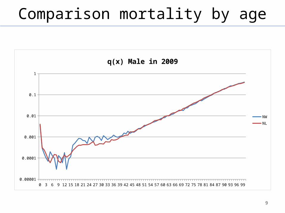
Comparison mortality by age

9

0 3 6 9 12 15 18 21 24 27 30 33 36 39 42 45 48 51 54 57 60 63 66 69 72 75 78 81 84 87 90 93 96 990.00001

0.0001

0.001

0.01

0.1

1

q(x) Male in 2009

NWNL

Comparison mortality by age

10

0 3 6 9 12 15 18 21 24 27 30 33 36 39 42 45 48 51 54 57 60 63 66 69 72 75 78 81 84 87 90 93 96 991

10

q(x) Female in 2009

NWNL

EXPLAINING THE HISTORY

11

Explaining the history

• (1) The “Hump”– In the early 50ts for the ages 45-75 for male the mortality

rates went up. This was caused by:• Smoking of cigarettes• Traffic accidents• Heart failure

– All these impacts are the result of behaviour• Smoking• Eating habits in combination with less healthy exercise habits• More driving in cars

– This flat period of development make the insurers not aware of the potential longevity risk in their portfolio

12

Explaining the history

• (1) The “Hump” (cont.)– During the seventies all three causes changed• Less smoking for male • Traffic get safer (in 1969 yearly more than 3000 traffic

deaths in NL, nowadays around 600)• Medical developments regarding heart attacks in

combination with a healthier way of living (healthier food, more exercise)

– … and the mortality rates went down again

13

Explaining the history

• (2) Trend change in 2001– The increase of the life expectancy suddenly went

up to more than 0.3 years per year (before that between 0.15 and 0.2), both for male and female

– Happened in almost the whole Western World– Reasons• Continuation of less smoking (particularly male)• Angioplasty as a treatment in case of an heart attack.

This increased the survival chance dramatically

14

Mortality development

• The development of life expectancy depends on:– Medical development

• And is it available?

– Behaviour• Drinking, smoking, eating habits,...

– Environment• Drinking water, one of the most important reasons of the increase of the life expectancy

in the developed countries• Pollution

– Water, air

• Climate– And so climate change

– New diseases– Resistance against medicines (antibiotics)

15

We can split development in 3 parts:

1850 1856 1862 1868 1874 1880 1886 1892 1898 1904 1910 1916 1922 1928 1934 1940 1946 1952 1958 1964 1970 1976 1982 1988 1994 2000 200630

40

50

60

70

80

90

Life expectancy at age zero, Netherlands

Male Female

2

16

1

3

We can split development in 3 parts

• (1) – No development of e(0)– High volatility• People less protected against extreme weather, flu

epidemics• Tuberculosis

– High mortality for young children• In 1850: e(0) male: 38.3; e(5) male: 50.8!

– Comparable with the underdeveloped countries

17

We can split development in 3 parts

• (2)– After the industrial revolution– Steep increase of life expectancy• Medical developments• Cleaner drinking water

– Seen as THE most important reason for improvement

• Environment – Better protection: heating in houses, toilets etc.

• Comparable with emerging countries

18

We can split development in 3 parts

• (3)– Typical for developed countries– Developments like the quality of drinking water are

reaching the limits– Change in life expectancy depends more of:

• Behaviour• Medical developments

– Both can have positive or negative effects.– Particularly behaviour can cause more independency

in development between male and female.

19

TRENDS, HOW TO MODEL?

20

How to model?

• In (1) and (2) it is rather easy to predict the future using the history

• In (3) this is very complex. History can hardly be use as dataset to predict the future.– More shocks (like in 2001) can be expected – Also a decrease of life expectancies is possible in the

coming 50 years:• Climate change • Resistance of antibiotics.• Behaviour (obesities)• …

21

How to model?

• In practice we see also a movement from (2) to (3) – for example in Central European Countries.

22

How old can a human become?

• The oldest confirmed human became 122 years and 164 days

• Jeanne Calment• Born: 25 February 1875• Secret?

• On all her food olive oil• Port wine diet• 1 kg of chocolate a week

23

How old can a human become?

• It cannot be proven that the max age is increasing

• Medical experts mention that a real life span exist per person, depending on the genetic passport, but will be limited to around 125-130 years.

• Mortality rates seem to be almost constant above age 105 at a level 0.5-0.6.

24

Conclusion (from my side)

• Pure mathematical models to predict the future mortality are less accurate

• Expert judgment is always needed for several decisions moments– Particularly input from the medical world is

needed• There is also a risk that the life expectancies

are getting lower than expected

25

Some models

• Based on cause of death:– Very complex, impossible without medical input• And many expert judgement decisions

– Information used not always reliable (>80)– Correlation between causes of death

– Models limited to 10 years projection

26

Some models

• By structure:– Separate models for • Very young children (under age 5)• Accident hump (age 18-25)• Aging (exponential model)• Age independent part

– Lots of parameters needed. This makes it hard to estimate and control

27

Some models

• Linear models like Lee Carter – Most likely too simple

• Short term – long term trend modelling– goal table approach– Good experience on the short term– Long term trend needs expert judgment

• Linear with adjustments for behaviour– CBS 2012: Average Western European mortality

adjusted for smoking behaviour 28

NEW STOCHASTIC TREND MODEL

29

New stochastic model

• Recently developed a new stochastic model for trend uncertainty

• This model is based on a multi-drift simulation, not the one-year volatility.

• Creates both one-year risk as multi-year risk measurements

30

New stochastic model

• Like in Lee Carter mortality development can be split in a drift plus a one year volatility.

• Other than in LC the volatility is not used to project future mortality, but the drift is analysed.

• To reduce the volatility a two-years average is taken– Volatility should be modelled as a separate sub-

risk (later more)31

New stochastic model

• The period we are analysing is first split into 16 years periods

• Each 16-year period is split into 2 8-year periods

• Each 8-year period is split into 2 4-year periods

• Each 4-year period is split into 2 2-year periods.

32

Example16 year drift

33

Example16 year drift

34

Example8 year drift

35

Example8 year drift

36

Then the same exercise for

How to use?

• Now we have many scenario’s • Before going into a simulation these scenario’s

are translated into the measurement we want: e.g. life expectancy or liabilities over a portfolio

• In this way dependencies are taken into account• The distributions are defined around the life

expectancies or liabilities– For the e(0) in this presentation I used Normal, with

some (negative) skewness

37

Results of the new model

38

195119551959196319671971197519791983198719911995199920032007201120152019202320272031203520392043204720512055205965

70

75

80

85

90

95

100

Male, history + futureDutch data

e(0)

First outcomes

20122014

20162018

20202022

20242026

20282030

20322034

20362038

20402042

20442046

20482050

20522054

20562058

206070

75

80

85

90

95

100

E(0) analyses met drift trend modelsimultie obv drifts 5000 simulatie scenarios

Based in Dutch data

95%BECBS95%90%99.50%Vaupel

39

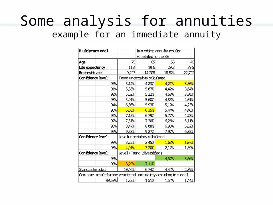
Some analysis for annuitiesexample for an immediate annuity

Age 75 65 55 45Life expectency 11,4 19,6 29,3 39,9

9,223 14,208 18,824 22,722

90% 5,14% 4,83% 4,21% 3,50%91% 5,38% 5,07% 4,42% 3,64%92% 5,62% 5,32% 4,63% 3,80%93% 5,91% 5,60% 4,85% 4,01%94% 6,30% 5,93% 5,10% 4,23%95% 6,68% 6,35% 5,44% 4,46%96% 7,15% 6,79% 5,77% 4,73%97% 7,81% 7,30% 6,26% 5,11%98% 8,47% 8,08% 6,95% 5,62%99% 9,53% 9,27% 7,97% 6,35%

90% 3,75% 2,45% 1,63% 1,07%95% 4,91% 3,20% 2,12% 1,39%

90% 4,52% 3,66%95% 8,29% 7,11%

10,46% 6,74% 4,44% 2,89%

99,50% 1,33% 1,51% 1,54% 1,44%Compare: result for one year trend uncertainty according to model

Multi year model Immediate annuity results:EC related to the BE

Best estimateConfidence level: Trend uncertainty calculated

Confidence level: Level uncertainty calculated

Confidence level: Level + Trend (diversified)

Standard model

INTERNATIONAL VIEW

41

International view

• Following the ideas countries that are in situation 3 should have comparable trend developments (save development level)

• Also following several studies the uncertainty should be comparable over the countries (I would like to add under the same circumstances) and can be used in case a lack of data exist in a country– Li Lee – CBS

42

Countries in (3)

43

Countries in (3)

44

Countries in (3)Model outcomes for male

45

2012 BE 2060 2060 incl. 95% unc.95% uncertaintyAUSTRIA 78.24 88.13 92.66 4.53BELGIUM 77.78 86.28 90.80 4.52DENMARK 77.82 87.17 92.34 5.17FRANCE 78.62 88.46 92.50 4.04ITALY 79.96 88.66 93.78 5.13NETHERLANDS 79.28 87.85 92.82 4.97NORWAY 79.36 87.77 92.77 5.00UK 78.99 89.39 93.19 3.80USA 76.84 85.91 89.95 4.04SWISS 80.57 89.27 92.80 3.53SWEDEN 79.97 87.24 90.53 3.29

Countries in (3)Model outcomes for male

46

Conclusions

• Indeed the uncertainty results of comparable countries are indeed close, but:– Larger countries have a somewhat lower

uncertainty (still some volatility left?)– Need to look at Sweden and Swiss

47

OTHER MORTALITY RISKS

48

Other risks

• Beside trend uncertainty mortality risk also contains:– Volatility– Level uncertainty– Calamity (extreme event)

49

Volatility

• Volatility because of “whole population issues” is based on a dependency in mortality because of for example– Appearance or non-appearance of Cold winters– Appearance or non-appearance of Hot summers– Seasonal flu epidemics– Severe accidents or natural disasters– Extreme events like a pandemic– … other ?

Volatility

• Also within the whole population mortality there will be a random effect, particularly because mortality rates are set by age/gender.– This part of the volatility is not part of the

mortality risk to be modelled• The random effect is measured in the insured

population involved.

Level uncertainty

• Level uncertainty should cover the statistical uncertainty in translating whole population mortality (or mortality based on some reference table) into mortality for the specific insured group.

52

EXTREME EVENTS, PANDEMICS

53

• For mortality extreme event modelling is generally based on a pandemic scenario.– E.g. in Solvency II the Spanish Flu is translated into

the modern times.• But…

How to model: extreme events

• But…• A pandemic risk is not a constant over time– Risk situation changes over time– This is measured in the WHO pandemic ratio– Solvency II• In general once in 40 years a pandemic• 1 in the 5 of them is worse enough to be a a “Solvency

II shock” • But this is measured in case WHO ratio is 1!

How to model: extreme events

• But the WHO 1 level was always higher than 1– In general 3.

• So what is the 1 in 200 scenario

• Perhaps better to talk about a scenario instead of 1 in 200.– Scenario can be the Spanish flu

How to model: extreme events

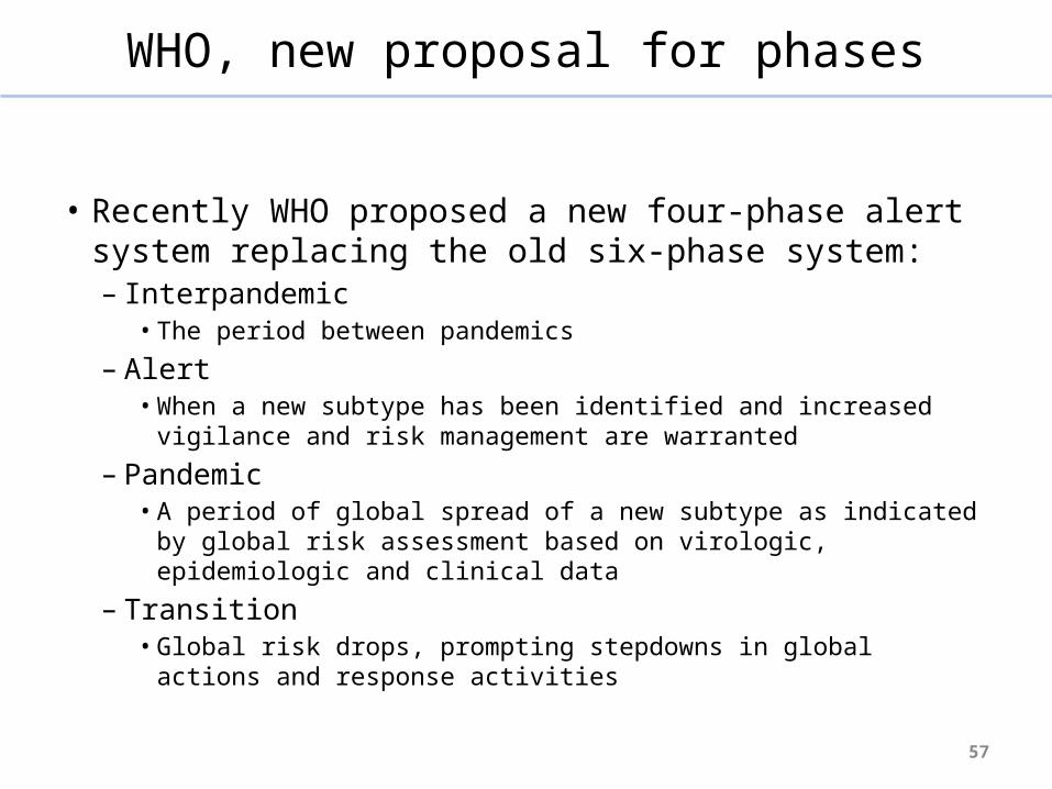
WHO, new proposal for phases

• Recently WHO proposed a new four-phase alert system replacing the old six-phase system:– Interpandemic

• The period between pandemics

– Alert• When a new subtype has been identified and increased vigilance and

risk management are warranted

– Pandemic• A period of global spread of a new subtype as indicated by global risk

assessment based on virologic, epidemiologic and clinical data

– Transition• Global risk drops, prompting stepdowns in global actions and response

activities

57

Conclusion

• Particularly for modelling extreme events we should look more at “conditional” modelling

58

59

Det er det ....

Takk