understanding index option returns - columbia university

Understanding Index Option Returns

Mark BroadieColumbia University

Mikhail ChernovLondon Business School and CEPR

Michael JohannesColumbia University

Previous research concludes that options are mispriced based on the high average returns,CAPM alphas, and Sharpe ratios of various put selling strategies. One criticism of theseconclusions is that these benchmarks are ill suited to handle the extreme statistical natureof option returns generated by nonlinear payoffs. We propose an alternative way to evaluatethe statistical significance of option returns by comparing historical statistics to thosegenerated by option pricing models. The most puzzling finding in the existing literature,the large returns to writing out-of-the-money puts, is not inconsistent (i.e., is statisticallyinsignificant) relative to the Black-Scholes model or the Heston stochastic volatility modeldue to the extreme sampling uncertainty associated with put returns. This sampling problemcan largely be alleviated by analyzing market-neutral portfolios such as straddles or delta-hedged returns. The returns on these portfolios can be explained by jump risk premiumsand estimation risk. (JEL C12, G13)

It is a common perception that index options are mispriced, in the sense thatcertain option returns are excessive relative to their risks.1 The primary evidencesupporting mispricing is the large magnitude of historical S&P 500 put option

We thank David Bates, Alessandro Beber, Oleg Bondarenko, Peter Bossaerts, Pierre Collin-Dufresne, KentDaniel, Joost Driessen, Bernard Dumas, Silverio Foresi, Vito Gala, Toby Moskowitz, Lasse Pedersen, MirelaPredescu, Todd Pulvino, Alex Reyfman, Alessandro Sbuelz, and Christian Schlag for helpful comments. Thispaper was presented at the Adam Smith Asset Pricing conference, the 2008 AFA meetings in New Orleans,the Amsterdam Business School, AQR Capital Management, College of Queen Mary, Columbia, the ESSFMmeetings in Gerzensee, the Fields Institute in Toronto, Goldman Sachs Asset Management, HEC-Lausanne, HEC-Montreal, Lugano, Manchester Business School, Minnesota, the NBER Summer Institute, Tilburg, UniversidadeNova de Lisboa, the 2nd Western Conference in Mathematical Finance, and the Yale School of Management.We thank Sam Cheung, Sudarshan Gururaj, and Pranay Jain for research assistance. We are grateful to theanonymous referee and to the editor, Matthew Spiegel, whose comments resulted in significant improvements inthe paper. Broadie acknowledges support by the National Science Foundation, grant no. DMS-0410234. Chernovacknowledges support by the BNP Paribas Hedge Funds Centre. Broadie and Chernov acknowledge support bythe JP Morgan Chase Academic Outreach program. Send correspondence to Mikhail Chernov, London BusinessSchool, Regent’s Park, London NW1 4SA, United Kingdom. E-mail: [email protected].

1 At this stage, a natural question is why to focus on returns and not option prices, Returns, as opposed to pricelevels, are typically analyzed because of their natural economic interpretation. Returns represent actual gains orlosses on purchased securities. In contrast, common option pricing exercises use pricing errors to summarizefit, which are neither easily interpreted nor can be realized. In addition, we have stronger intuition about return-based measures such as excess returns, CAPM alphas, or Sharpe ratios as compared to pricing errors. Coval andShumway (2001) provide additional motivation.

C© The Author 2009. Published by Oxford University Press on behalf of The Society for Financial Studies.All rights reserved. For Permissions, please e-mail: [email protected]:10.1093/rfs/hhp032

RFS Advance Access published May 4, 2009

The Review of Financial Studies

returns. For example, Bondarenko (2003) reports that average at-the-money(ATM) put returns are −40%, not per annum, but per month, and deep out-of-the-money (OTM) put returns are −95% per month. Average option returnsand CAPM alphas are statistically significant, with p-values close to zero, andSharpe ratios are larger than those of the underlying index.2

There are three obvious factors to consider when interpreting these results.Option returns are highly nonnormal and metrics assuming normality, suchas CAPM alphas or Sharpe ratios, are inappropriate.3 Additionally, averageput returns should be negative due to the leverage inherent in options and thepresence of priced risks. Finally, options have only traded for a short periodof time, and it is difficult to assess the statistical significance of option returnsdue to the short time spans and nonnormality of option returns. Together, thesefactors raise questions about the usual procedures of applying standard assetpricing metrics to analyze option returns.

In this paper, we use option pricing models as a benchmark to assess theevidence for index option mispricing and address the issues raised above.Option returns computed from formal option pricing models automaticallyreflect the leverage and kinked payoffs of options, anchor hypothesis testsat appropriate null values, provide a framework for assessing the impact ofrisk premiums, and provide a mechanism for assessing statistical uncertaintyvia finite-sample simulations. Ideally, an equilibrium model over economicfundamentals, such as consumption or dividends, would be used to assess theevidence for mispricing. However, as argued by Bates (2008) and Bondarenko(2003), such an explanation is extremely challenging inside the representativeagent framework. This is not a surprise, since these models have difficultiesexplaining not only the low-frequency features of stock returns (e.g., the equitypremium or excess volatility puzzles) but also high-frequency movements suchas price jumps, high-frequency volatility fluctuations, or the leverage effect.

We address a more modest, but still important, goal of understanding the pric-ing of options relative to the underlying index, as opposed to pricing options rel-ative to the underlying fundamental variables. To do this, we use affine-jump dif-fusion models of stock index returns. These models account for the key driversof equity returns and option prices such as diffusive price shocks, stochasticvolatility, and price jumps. The key step is one of calibration: we calibrate eachmodel to fit the observed behavior of equity index returns over the sample forwhich option returns are available. In particular, this approach implies that ourmodels replicate the historically observed equity premium and volatility.

2 The returns are economically significant, as investors endowed with a wide array of utility functions find largecertainty equivalent gains from selling put options (e.g., Driessen and Maenhout 2004b; Santa-Clara and Saretto2007).

3 The shortcomings of these metrics have been understood for a long time (see Glosten and Jagannathan 1994;Goetzmann et al. 2007; Grinblatt and Titman 1989; and Leland 1999, among others). However, their use is stillpervasive both in the industry and in academia.

2


Methodologically, we proceed using two main tools. First, we show thatexpected option returns (EORs) can be computed analytically, allowing us toexamine the quantitative impact of different factors and parameter values onoption returns. In particular, EORs anchor null hypothesis values when testingwhether average option returns are significantly different from those generatedby a given null model. Second, we simulate index sample paths to constructexact finite-sample distributions for the statistics analyzed. This procedureaccounts for both the small sample sizes (on the order of 200 months) andthe highly skewed and nonnormal nature of option return distributions. It alsoallows us to assess the statistical uncertainty of commonly used asset pricingbenchmarks and statistics, such as average returns, CAPM alphas, or Sharperatios.4

Empirically, we present a number of interesting findings. We first analyze putreturns, given their importance in the recent literature, and begin with the stan-dard Black and Scholes (1973) and Heston (1993) stochastic volatility models.Although these models are too simple to accurately describe option prices, theyprovide key insights for understanding and evaluating option returns. Our firstresult is that average returns, CAPM alphas, and Sharpe ratios for deep OTMput returns are statistically insignificant when compared to the Black-Scholesmodel. Thus, one of the most puzzling statistics in the literature, the largeaverage OTM put returns, is not inconsistent with the Black-Scholes model.Moreover, there is little evidence that put returns of any strike are inconsistentwith Heston’s (1993) stochastic volatility (SV) model, assuming no diffusivestochastic volatility risk premiums (i.e., the evolution of volatility under theobjective, P, and the risk-neutral, Q, measures are the same).

We interpret these findings not as evidence that the Black-Scholes or Hestonmodels are correct—we know they can be rejected on other grounds—but ratheras highlighting the statistical difficulties present when analyzing option returns.Short samples and complicated option return distributions imply that standardstatistics are so noisy that little can be concluded by analyzing option returns.It is well known that it is difficult to estimate the equity premium, and thisuncertainty is only magnified when estimating average put returns.

This implies that tests using put option returns are not very informative aboutoption mispricing, and we next turn to returns of alternative option portfoliostrategies such as ATM straddles, crash-neutral straddles, covered puts, putspreads, and delta-hedged puts. These portfolios are more informative becausethey either reduce the exposure to the underlying index (straddles and delta-hedged puts) or dampen the effect of rare events (crash-neutral straddles andput spreads).

Of all of these portfolios, straddles are quite useful since straddles do notrequire a model to determine the initial portfolio position (unlike delta-hedged

4 The results are similar using alternative measures, such as Leland’s alpha (Leland 1999) or the manipulationproof performance measure (Goetzmann et al. 2007).

3


puts) and the returns are approximately market neutral. Straddles are also moreinformative than individual puts, since average straddle returns are highly sig-nificant when compared to returns generated from the Black-Scholes modelor a baseline stochastic volatility model without a diffusive volatility risk pre-mium. The source of this significance is the well-known wedge between theATM-implied volatility and the subsequent realized volatility.5 As argued byPan (2002) and Broadie, Chernov, and Johannes (2007), it is unlikely that a dif-fusive stochastic volatility risk premium could generate this wedge because theoptions are short-dated, and a stochastic volatility risk premium would mainlyimpact longer-dated options.

We consider two mechanisms to generate wedges between realized and im-plied volatility in jump-diffusion models: jump risk premiums and estimationrisk. The jump risk explanation uses the jump risk corrections implied by anequilibrium model as a simple device for generating Q-measure jump parame-ters, given P-measure parameters. Consistent with our original intent, such anadjustment does not provide an equilibrium explanation, as we calibrate theunderlying index model to match the overall equity premium and volatility ofreturns. In the case of estimation risk, we assume that investors account for theuncertainty in spot volatility and parameters when pricing options.

Both of these explanations generate option returns that are broadly consistentwith those observed historically. For example, average put returns are matchedpointwise and the average returns of straddles, put spreads, crash-neutral strad-dles, and delta-hedged portfolios are all statistically insignificant.

These results indicate that, at least for our parameterizations, option returnsare not puzzling relative to the benchmark models. Option and stock returnsmay remain puzzling relative to consumption and dividends, but there is littleevidence for mispricing relative to the underlying stock index.

The rest of the paper is outlined as follows. Section 1 outlines our method-ological approach. Section 2 discusses our dataset and summarizes the evidencefor put mispricing. Section 3 illustrates the methodology based on the Black-Scholes and Heston models. Section 4 investigates strategies based on optionportfolios. Section 5 illustrates how a model with stochastic volatility and jumpsin prices generate realistic put and straddle returns. Conclusions are given inSection 6.

1. Our Approach

We analyze returns to a number of option strategies. In this section, we discusssome of the concerns that arise in analyzing option returns, and then discuss ourapproach. To frame the issues, we focus on put option returns, but the resultsand discussion apply more generally to portfolio strategies such as put spreads,straddles, or delta-hedged returns.

5 Over our sample, ATM-implied volatility averaged 17% and the realized volatility was 15%.

4


Hold-to-expiration put returns are defined as

r pt,T = (K − St+T )+

Pt,T (K , St )− 1, (1)

where x+ ≡ max(x, 0) and Pt,T (K , St ) is the time-t price of a put option writtenon St , struck at K , and expiring at time t + T . Hold-to-expiration returns aretypically analyzed both in academic studies and in practice for two reasons.First, option trading involves significant costs, and strategies that hold untilexpiration incur these costs only at initiation. For example, ATM (deep OTM)index option bid-ask spreads are currently on the order of 3–5% (10%) of theoption price. The second reason, discussed fully in Section 2, is that high-frequency option returns generate a number of theoretical and statistical issuesthat are avoided using monthly returns.

The goal of this literature is to assess whether or not option returns areexcessive, either in absolute terms or relative to their risks. Existing approachesrely on statistical models, as discussed in Appendix A. For example, it iscommon to compute average returns, CAPM alphas, or Sharpe ratios. Strategiesthat involve writing options generally deliver higher average returns than theunderlying asset, have economically and statistically large CAPM alphas, andhave higher Sharpe ratios than the market.

How should these results be interpreted? Options are effectively leveragedpositions in the underlying asset (which typically has a positive expected re-turn), so call (put) options have higher (lower) expected returns than the un-derlying. For example, expected put option returns are negative, which impliesthat standard t-tests of average option returns that test the null hypothesis thataverage returns are zero are improprely anchored. The precise magnitude ofexpected returns depends on a number of factors that include the specific model,the parameters, and factor risk premiums. In particular, EORs are very sensitiveto both the equity premium and volatility.

It is important to control for the option’s exposure to the underlying, which iscommonly done by computing betas using a CAPM-style specification. This ap-proach is motivated by the hedging arguments used to derive the Black-Scholesmodel. According to this model, the link between instantaneous derivativereturns and excess index returns is

df (St )

f (St )= rdt + St

f (St )

∂ f (St )

∂St

[dSt

St− (r − δ) dt

], (2)

where r is the risk-free rate, f (St ) the derivative price, and δ the divi-dend rate on the underlying asset. This implies that instantaneous changesin the derivative’s price are linear in the index returns, d St/St , and instanta-neous option returns are conditionally normally distributed. This instantaneous

5


CAPM is often used to motivate an approximate linear factor model for optionreturns

f (St+T ) − f (St )

f (St )= αt,T + βt,T

(St+T − St

St− rT

)+ εt,T .

These linear factor models are used to adjust for leverage, via βt,T , and asa pricing metric, via αt,T . In the latter case, αT �= 0 is often interpreted asevidence of either mispricing or risk premiums.

As shown empirically and theoretically in Appendix B, standard optionpricing models (including the Black-Scholes model) generate population valuesof αt,T that are different from zero.6 In the Black-Scholes model, this is dueto time discretization, but in more general jump-diffusion models, αt,T can benonzero for infinitesimal intervals due to the presence of jumps. This impliesthat it is inappropriate to interpret a nonzero αt,T as evidence of mispricing.Similarly, Sharpe ratios account for leverage by scaling average excess returnsby volatility, which provides an appropriate metric when returns are normallydistributed or if investors have mean-variance preferences. Sharpe ratios areproblematic in our setting because option returns are highly nonnormal, evenover short time intervals.

Our approach is different. We view these intuitive metrics (average returns,CAPM alphas, and Sharpe ratios) through the lens of formal option pric-ing models. The experiment we perform is straightforward: we compare theobserved values of these statistics in the data to those generated by optionpricing models such as Black-Scholes and extensions incorporating jumps orstochastic volatility. The use of formal models plays two roles: it provides anappropriate null value for anchoring hypothesis tests, and it provides a mech-anism for dealing with the severe statistical problems associated with optionreturns.

1.1 ModelsWe consider nested versions of a general model with mean-reverting stochasticvolatility and lognormally distributed Poisson-driven jumps in prices. Thismodel, proposed by Bates (1996) and Scott (1997) and referred to as the SVJmodel, is a common benchmark (see, e.g., Andersen, Benzoni, and Lund 2002;Bates 1996; Broadie, Chernov, and Johannes 2007; Chernov et al. 2003; Eraker2004; Eraker, Johannes, and Polson 2003; Pan 2002). As special cases of themodel, we consider the Black and Scholes (1973) model, the Merton (1976)jump-diffusion model, and the Heston (1993) stochastic volatility model.

6 Leland (1999) makes this point in the context of the Black-Scholes model.

6


The model assumes that the ex-dividend index level St and its spot varianceVt evolve under the physical (or real-world) P-measure according to

dSt = (r + μ − δ)St dt + St

√Vt dWs

t (P)

+ d

⎛⎝Nt (P)∑

j=1

Sτ j−[eZs

j (P) − 1]⎞⎠ − λPμPSt dt, (3)

dVt = κPv

(θPv − Vt

)dt + σv

√Vt dWv

t (P), (4)

where r is the risk-free rate, μ is the cum-dividend equity premium,δ is the dividend yield, W s

t and W vt are two correlated Brownian mo-

tions (E[W st W v

t ] = ρt), Nt (P) ∼ Poisson (λPt), Zsj (P) ∼ N (μP

z , (σPz )2), and

μP = exp (μPz + (σP

z )2/2) − 1. Black-Scholes is a special case with no jumps(λP = 0) and constant volatility (V0 = θP

v , σv = 0), Heston’s model is a spe-cial case with no jumps, and Merton’s model is a special case with constantvolatility. When volatility is constant, we use the notation

√Vt = σ.

Options are priced using the dynamics under the risk-neutral measure Q:

dSt = (r − δ)St dt + St

√Vt dWs

t (Q)

+ d

⎛⎝Nt (Q)∑

j=1

Sτ j−[eZs

j (Q) − 1]⎞⎠ − λQμQSt dt, (5)

dVt = κQv

(θQv − Vt

)dt + σv

√Vt dWv

t (Q), (6)

where Nt (Q) ∼ Poisson (λQt), Z j (Q) ∼ N (μQz , (σQ

z )2), Wt (Q) are Brownianmotions, and μQ is defined analogously to μP. The diffusive equity premiumis μc, and the total equity premium is μ = μc + λPμP − λQμQ. We generallyrefer to a nonzero μ as a diffusive risk premium. Differences between the risk-neutral and real-world jump and stochastic volatility parameters are referred toas jump or stochastic volatility risk premiums, respectively.

Both the parameters θv and κv can potentially change under the risk-neutralmeasure (Cheredito, Filipovic, and Kimmel 2007). We explore changes in θP

v

and constrain κQv = κP

v , because, as discussed below, average returns are notsensitive to empirically plausible changes in κP

v . Changes of measure for jumpprocesses are more flexible than those for diffusion processes. We assume thatthe jump size distribution is lognormal under Q with potentially different meansand variances. Below we discuss in detail two mechanisms, risk premiums andestimation risk, to calibrate the risk-neutral parameters.

1.2 Methodological frameworkMethodologically, we rely on two main tools: analytical formulas for expectedreturns and Monte Carlo simulation to assess statistical significance.

7


1.2.1 Analytical expected option returns. Expected put option returns aregiven by

EPt

(r p

t,T

) = EPt [(K − St+T )+]

Pt,T (St , K )− 1 = EP

t [(K − St+T )+]

EQt [e−rT (K − St+T )+]

− 1. (7)

From this expression, it is clear that any model that admits “analytical” optionprices, such as affine models, will allow EORs to be computed explicitly sinceboth the numerator and denominator are known analytically. Higher momentscan also be computed. Surprisingly, despite a large literature analyzing optionreturns, the fact that EORs can be easily computed has neither been noted norapplied.7

EORs do not depend on St . To see this, define the initial moneyness of theoption as κ = K/St . Option homogeneity implies that

EPt

(r p

t,T

) = EPt [(κ − Rt,T )+]

EQt [e−rT (κ − Rt,T )+]

− 1, (8)

where Rt,T = St+T /St is the gross index return.8 EORs depend only on themoneyness, maturity, interest rate, and distribution of index returns.9

This formula provides exact EORs for finite holding periods regardless of therisk factors of the underlying index dynamics and without using CAPM-styleapproximations. These analytical results are primarily useful as they allow usto assess the exact quantitative impact of risk premiums or parameter config-urations. Equation (7) implies that the gap between the P and Q probabilitymeasures determines EORs, and the magnitude of the returns is determined bythe relative shape and location of the two probability measures.10 In modelswithout jump or stochastic volatility risk premiums, the gap is determined bythe fact that the P and Q drifts differ by the equity risk premium. In modelswith priced stochastic volatility or jump risk, both the shape and location ofthe distribution can change, leading to more interesting patterns of expectedreturns across different moneyness categories.

7 This result is closely related to that of Rubinstein (1984), who derived it specifically for the Black-Scholes caseand analyzed the relationship between hold-to-expiration and shorter holding period expected returns.

8 Glosten and Jagannathan (1994) use option homogeneity to benchmark payoff from one dollar invested in amutual fund with unknown asset composition against a portfolio consisting of the index with a payoff of Rt,T

and an option with a payoff (Rt,T − κ)+. Subsequently, Glosten and Jagannathan use the Black-Scholes modelto value the benchmark portfolio.

9 When stochastic volatility is present in a model, the expected option returns can be computed analyticallyconditional on the current variance value: EP(r p

t,T |Vt ). The unconditional expected returns can be computedusing iterated expectations and the fact that

EP(r p

t,T

) =∫

EP(r p

t,T |Vt)

p (Vt ) dVt .

The integral can be estimated via Monte Carlo simulation or by standard deterministic integration routines.

10 For monthly holding periods, 1 ≤ exp (rT ) ≤ 1.008 for 0% ≤ r ≤ 10% and T = 1/12 years, so the discountfactor has a negligible impact on EORs.

8


1.2.2 Finite-sample distribution via Monte Carlo simulation. To assessstatistical significance, we use Monte Carlo simulation to compute the distribu-tion of various returns statistics, including average returns, CAPM alphas, andSharpe ratios. We are motivated by concerns that the use of limiting distribu-tions to approximate the finite-sample distribution is inaccurate in this setting.Our concerns arise due to the relatively short sample and extreme skewnessand nonnormality of option returns.

To compute the finite-sample distribution of various option return statistics,we simulate N = 215 months (the sample length in the data) of index levelsG = 25,000 times using standard simulation techniques. For each month andindex simulation trial, put returns for a fixed moneyness are

r p,(g)t,T =

(κ − R(g)

t,T

)+

PT (κ)− 1, (9)

where

PT (κ) � Pt,T (St , K )

St= e−rT EQ

t [(κ − Rt,T )+],

t = 1, . . . , N and g = 1, . . . , G. Average option returns for simulation g usingN months of data are

r p,(g)T = 1

N

∑N

t=1r p,(g)

t,T .

The set of G average returns forms the finite-sample distribution. Similarly, wecan construct finite-sample distributions for Sharpe ratios, CAPM alphas, andother statistics of interest for any option portfolio.

This parametric bootstrapping approach provides exact finite-sample infer-ence under the null hypothesis that a given model holds. It can be contrastedwith the nonparametric bootstrap, which creates artificial datasets by samplingwith replacement from the observed data. The nonparametric bootstrap, whichessentially reshuffles existing observations, has difficulties dealing with rareevents. In fact, if an event has not occurred in the observed sample, it will neverappear in the simulated finite-sample distribution. This is an important concernwhen dealing with put returns, which are sensitive to rare events.

1.3 Parameter estimationWe calibrate our models to fit the realized historical behavior of the underlyingindex returns over our observed sample. Thus, the P-measure parameters areestimated directly from historical index return data, and not consumption ordividend behavior. For parameters in the Black-Scholes model, this calibrationis straightforward, but in models with unobserved volatility or jumps, theestimation is more complicated, as it is not possible to estimate all of theparameters via simple sample statistics.

9


Table 1P-measure parameters √

θPv

√θPv

r μ λP μPz σP

z (SV) (SVJ) κPv σv ρ

4.50% 5.41% 0.91 −3.25% 6.00% 15.00% 13.51% 5.33 0.14 −0.52(0.34) (1.71) (0.99) (1.28) (0.84) (0.01) (0.04)

This table reports values of P-measure parameters that we use in our computational examples. Standard errorsfrom the SVJ estimation are reported in parentheses. Parameters are given in annual terms.

For all of the models that we consider, the interest rate and equity premiummatch those observed over our sample, r = 4.5% and μ = 5.4%. Since weanalyze futures returns and futures options, δ = r . In each model, we alsoconstrain the total volatility to match the observed monthly volatility of futuresreturns, which was 15%. In the most general model we consider, we do this byimposing that

√θPv + λP

((μP

z

)2 + (σP

z

)2) = 15%

and by modifying θPv appropriately. In the Black-Scholes model, we set the

constant volatility to be 15%.To obtain the values of the remaining parameters, we estimate the SVJ

model using daily S&P 500 index returns spanning the same time period asour options data, from 1987 to 2005. We use MCMC methods to simulate theposterior distribution of the parameters and state variables following Eraker,Johannes, and Polson (2003) and others. The parameter estimates (posteriormeans) and posterior standard deviations are reported in Table 1. The parameterestimates are in line with the values reported in previous studies (see Broadie,Chernov, and Johannes 2007 for a review).

Of particular interest for our analysis are the jump parameters. The estimatesimply that jumps are relatively infrequent, arriving at a rate of about λP = 0.91per year. The jumps are modestly sized with a mean of −3.25% and a standarddeviation of 6%. Given these values, a “two sigma” downward jump size willbe equal to −15.25%. Therefore, a crash-type move of −15% or less will occurwith a probability of λP·5%, or approximately once in twenty years.

As we discuss in greater detail below, estimating jump intensities and jumpsize distributions is extremely difficult. The estimates are highly dependent onthe observed data and on the specific model. For example, different estimateswould likely be obtained if we assumed that the jump intensity was dependenton volatility (as in Bates 2000 or Pan 2002) or if there were jumps in volatility.Again, our goal is not to exhaustively analyze every potential specification butrather to understand option returns in common specifications and for plausibleparameter values.

We discuss the calibration of Q-measure parameters later. At this stage,we only emphasize that we do not use options data to estimate any of the

10


parameters. Estimating Q-parameters from option prices for use in understand-ing observed option returns would introduce a circularity, as we would beexplaining option returns with information extracted from option prices.

2. Initial Evidence for Put Mispricing

We collect historical data on S&P 500 futures options from August 1987 toJune 2005, a total of 215 months. These options are American, but our statisticsare computed using the European values estimated through the procedure fromBroadie, Chernov, and Johannes (2007). This sample is considerably longerthan those previously analyzed and starts in August of 1987, when one-month“serial” options were introduced. Contracts expire on the third Friday of eachmonth, which implies there are 28 or 35 calendar days to maturity dependingon whether it was a four- or five-week month. We construct representative dailyoption prices using the approach in Broadie, Chernov, and Johannes (2007);details of this procedure are given in Appendix C.

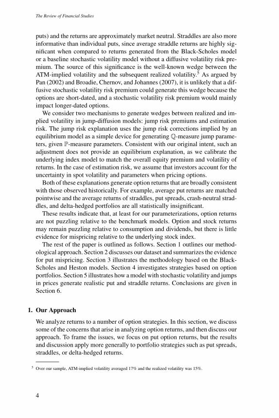
Using these prices, we compute option returns for fixed moneyness, measuredby strike divided by the underlying, ranging from 0.94 to 1.02 (in 2% incre-ments). This range covers the most actively traded options (85% of one-monthoption transactions occur in this range). We did not include deeper OTM or ITMstrikes because of missing values. Payoffs are computed using settlement valuesfor the S&P 500 futures contract. Figure 1 shows the time series for 6% OTMand ATM put returns, highlighting some of the issues present when evaluatingthe statistical significance of statistics generated by option returns. Put returnshave infrequent but very large values and many repeated values, since OTMexpirations generate returns of −100%. We also compute returns for a range ofportfolio strategies, including covered puts, put spreads (crash-neutral put port-folios), ATM and crash-neutral straddles, and delta-hedged puts. We first con-sider raw put returns, as this has been the primary focus in the existing literature.

As mentioned earlier, we use hold-to-maturity returns. The alternative wouldbe higher frequency returns, weekly or even daily. The intuition for consider-ing high-frequency returns comes from Black-Scholes dynamic hedging ar-guments, indicating that option returns become approximately normal overhigh frequencies. Appendix D describes the difficulties associated with high-frequency option returns. In summary, we argue that high-frequency returnsgenerate additional theoretical, data, and statistical problems. In particular,simulation evidence shows that moving from monthly to weekly returns exac-erbates the statistical issues because the distribution of average returns becomeseven more nonnormal and dispersed.

The first piece of evidence commonly cited supporting mispricing is thelarge magnitude of the returns. According to Table 2, average monthly returnsare −57% for 6% OTM strikes (i.e., K/S = 0.94) and −30% for ATM strikesand are statistically different from zero since the p-values are close to zero. Inparticular, to check that our results are consistent with previous findings, we

11


1988 1990 1992 1994 1996 1998 2000 2002 2004 2006

−100

200

500

800

1100

1400%

pe

r m

on

th

(a) 6% OTM put returns

1988 1990 1992 1994 1996 1998 2000 2002 2004 2006

−100

200

500

800

% p

er

mo

nth

(b) ATM put returns

Figure 1Time series of options returns.

Table 2Average put option returns

Moneyness 0.94 0.96 0.98 1.00 1.02

08/1987 to 06/2005 −56.8 −52.3 −44.7 −29.9 −19.0Standard error 14.2 12.3 10.6 8.8 7.1t-stat −3.9 −4.2 −4.2 −3.3 −2.6p-value, % 0.0 0.0 0.0 0.0 0.4Skew 5.5 4.5 3.6 2.5 1.8Kurt 34.2 25.1 16.7 10.5 7.1

Subsamples01/1988 to 06/2005 −65.2 −60.6 −51.5 −34.1 −21.601/1995 to 09/2000 −85.5 −71.6 −63.5 −50.5 −37.510/2000 to 02/2003 +67.2 +54.3 +44.5 +48.2 +40.408/1987 to 01/2000 −83.9 −63.2 −55.7 −39.5 −25.5

The first panel contains the full sample (215 monthly returns) results, with standard errors, t-statistics, p-values, and skewness and kurtosis statistics. The second panel analyzes subsamples. All relevant statistics are inpercentages per month.

compare our statistics to the one in the Bondarenko (2003) sample from 1987to 2000. The average returns are very close, but ours are slightly more negativefor every moneyness category except the deepest OTM category. Bondarenko(2003) uses closing prices and has some missing values. Our average returnsare slightly more negative than those reported for similar time periods bySanta-Clara and Saretto (2007).

12


Table 3Risk-corrected measures of average put option returns

Moneyness 0.94 0.96 0.98 1.00 1.02

CAPM α, % −48.3 −44.1 −36.8 −22.5 −12.5Std.err., % 11.6 9.3 7.1 4.8 2.9t-stat −4.1 −4.7 −5.1 −4.6 −4.2p-value, % 0.0 0.0 0.0 0.0 0.0

Sharpe ratio −0.27 −0.29 −0.29 −0.23 −0.18

The first panel provides CAPM α’s with standard errors and the second panel provides put option Sharpe ratios(as a reference, the monthly Sharpe ratio for the market over our time period was about 0.1). These quantitieswere computed based on the full sample of 215 monthly returns from August 1987 to June 2005. All relevantstatistics except for the Sharpe ratios are in percentages per month. Sharpe ratios are monthly. The p-values arecomputed under the (incorrect) null hypothesis that average option returns are equal to zero.

The bottom panel of Table 2 reports average returns over subsamples. Aver-age put returns are unstable over time. For example, put returns were extremelynegative during the late 1990s during the dot-com “bubble” but were positiveand large from late 2000 to early 2003. The subsample starting in January 1988provides the same insight: if the extremely large positive returns realized aroundthe crash of 1987 are excluded, returns are much lower. Doing so generates asample selection bias and clearly demonstrates a problem with tests using shortsample periods.11

Table 3 reports CAPM alphas and Sharpe ratios, which delever and/or risk-correct option returns to account for the underlying exposure. CAPM alphasare highly statistically significant, with p-values near zero. The Sharpe ratiosof put positions are larger than those on the underlying market. For example,the monthly Sharpe ratio for the market over our time period was about 0.1,and the put return Sharpe ratios are two to three times larger. Based largelyon this evidence and additional robustness checks, the literature concludes thatput returns are puzzling and options are likely mispriced. We briefly review therelated literature in Appendix A.

3. The Role of Statistical Uncertainty

This section highlights the difficulties of establishing mispricing based onhistorical put returns. To do this, we use the simplest option pricing models,the Black-Scholes and SV models. We show that expected returns are highlysensitive to the underlying equity premium and volatility and also document theextreme finite-sample problems associated with tests using returns of individualoptions. In particular, the biggest puzzle in the literature—the large deep OTMput returns—is not inconsistent with the Black-Scholes model.

11 In simulations of the Black-Scholes model, excluding the largest positive return lowers average put option returnsby about 15% for the 6% OTM strike. This outcome illustrates the potential sample selection issues and howsensitive option returns are to the rare but extremely large positive returns generated by events such as the crashof 1987.

13


Table 4Population expected returns in the Black-Scholes model

Moneyness

σ μ 0.94 0.96 0.98 1.00 1.02 1.04 1.06

4% −27.6 −22.5 −17.6 −13.3 −9.7 −6.9 −5.010% 6% −38.7 −32.2 −25.7 −19.7 −14.5 −10.5 −7.7

8% −48.3 −40.8 −33.1 −25.7 −19.2 −14.1 −10.4

4% −15.4 −13.0 −10.8 −8.8 −7.1 −5.6 −4.515% 6% −22.5 −19.2 −16.1 −13.2 −10.7 −8.6 −6.9

8% −29.1 −25.0 −21.1 −17.5 −14.3 −11.5 −9.3

4% −10.3 −8.9 −7.7 −6.5 −5.5 −4.6 −3.920% 6% −15.2 −13.3 −11.5 −9.9 −8.4 −7.1 −6.0

8% −20.0 −17.6 −15.3 −13.2 −11.2 −9.5 −8.1

The parameter μ is the cum-dividend equity premium and σ is the volatility. These parameters are reported onan annual basis; expected option returns are monthly percentages.

3.1 Black-ScholesIn this section, we analyze EORs in the Black-Scholes model and analyze thefinite-sample distribution of average option returns, CAPM alphas, and Sharperatios. Table 4 displays EORs computed by Equation (8). The cum-dividendequity premium ranges from 4% to 8% and volatility ranges from 10% to 20%.

The impact of μ is approximately linear and quantitatively large, as thedifference in EORs between high and low equity premiums is about 10% forATM strikes and larger for deep OTM strikes. Because of this, any historicalperiod that is “puzzling” because of high realized equity returns will generateeven more striking option returns. For example, the realized equity premiumfrom 1990 to 1999 was 9.4%, and the average volatility was only 13% over thesame period. If fully anticipated, these values would, according to Equation (8),generate 6% OTM and ATM EORs of about −40% and −23%, respectively,which are much lower than the EORs using the full sample equity premiumand volatility.

Option returns are sensitive to volatility. As volatility increases, expectedput option returns increase (i.e., become less negative). For example, for 6%OTM puts with μ = 6%, EORs change from −39% for σ = 10% to −15% forσ = 20%. Thus volatility has a quantitatively large impact that varies acrossstrikes. Unlike the approximately linear relationship between EORs and μ, therelationship between put EORs and volatility is concave. This concavity impliesthat fully anticipated time-variation in volatility results in more negative EORsthan that if volatility were constant at the average value.

EORs are extremely difficult to estimate. As a first illustration, the top panelin Figure 2 shows the finite-sample distribution for 6% OTM average putreturns constructed from 25,000 sample paths, each of length 215. The solidvertical line is the observed sample value. The upper panel shows the largevariability in average put return estimates: the (5%, 95%) confidence band is−65% to +28%. The figure also shows the marked skewness of the distributionof average monthly option returns, which is expected given the strong positive

14


−100 −50 0 50 100 1500

500

1000

1500

2000

Average monthly return (%)

−100 −50 0 50 100 1500

500

1000

1500

2000

Monthly CAPM alpha (%)

−0.5 −0.4 −0.3 −0.2 −0.1 0 0.10

5000

10000

Monthly Sharpe ratio

Figure 2Finite-sample distributionThis figure shows histograms of the finite-sample distribution of various statistics. The top panel provides thedistribution of average 6% OTM put returns, the middle panel 6% OTM put CAPM alphas, and the bottom panel6% OTM put Sharpe ratios. The distributions are computed using 25,000 artificial histories, 215 months each,simulated from the Black-Scholes model. The solid vertical line is the observed value from the data.

skewness of purchased put options. This also indicates that the distribution ofaverage put returns is not well approximated by a normal distribution, at leastin samples of this size.

Table 5 summarizes EORs and p-values corresponding to observed averagereturns for various strikes. Note first that put average returns increase withmoneyness, are negative, and therefore are less than the risk-free rate. Thesepatterns are consistent with the prediction derived in Coval and Shumway(2001) under general assumptions. However, because of the extreme noiseassociated with these statistics, it would be hard to use this monotonicity todiscern alternative explanations of options returns.

The p-values have increased dramatically relative to Table 2. For example,the p-values using standard t-statistics for the ATM options increase by roughlya factor of ten and by more than 10,000 for deep OTM put options. This dramaticincrease occurs for two reasons: our procedure (1) anchors the null hypothesisat values generated by the option pricing model and (2) accounts for the largesampling uncertainty in the distribution of average option returns.

Next, average 6% OTM option returns are not statistically different fromthose generated by the Black-Scholes model, with a p-value of just over 8%.Based only on the Black-Scholes model, we have our first striking conclusion:

15


Table 5Option returns, CAPM α’s, and Sharpe ratios

Moneyness 0.94 0.96 0.98 1.00

Average returns Data, % −56.8 −52.3 −44.7 −29.9BS EP,% −20.6 −17.6 −14.6 −12.0

p-value,% 8.1 1.7 0.4 2.2SV EP,% −25.8 −21.5 −17.5 −13.7

p-value,% 24.1 9.3 3.0 7.3

CAPM αs Data, % −48.3 −44.1 −36.8 −22.5BS EP,% −17.9 −15.3 −12.7 −10.4

p-value,% 12.6 2.7 0.3 1.2SV EP,% −23.6 −19.5 −15.8 −12.4

p-value,% 39.1 14.1 3.4 8.7

Sharpe ratios Data −0.27 −0.29 −0.29 −0.23BS EP −0.05 −0.07 −0.08 −0.09

p-value,% 4.9 1.9 1.2 4.0SV EP −0.04 −0.07 −0.09 −0.10

p-value,% 21.5 12.0 7.7 14.3

This table reports population expected option returns, CAPM α’s, and Sharpe ratios and finite-sample dis-tribution p-values for the Black-Scholes (BS) and stochastic volatility (SV) models. We assume that all riskpremiums (except for the equity premium) are equal to zero. The p-values are computed using the finite-sampledistributions of the respective statistics. The distributions were constructed from 25,000 simulated paths, eachwith 215 monthly observations.

deep OTM put returns are insignificant when compared to the Black-Scholesmodel. This is particularly interesting since the existing literature concludesthat deep OTM put options are the most anomalous or mispriced. We arriveat the exact opposite conclusion: there is no evidence that OTM put returnsare excessive. It is important to note that other strikes are still significant, withp-values below 5%.

Next, consider CAPM alphas, which are reported in the second panel ofTable 5. For every strike, the alphas are quite negative and their magnitudesare economically large, ranging from −18% for 6% OTM puts to −10% forATM puts. Although Black-Scholes is a single-factor model, the alphas arequite negative in population, which is expected, as discussed in Section 2. Thisshows the fundamental problem that arises when applying linear factor modelsto nonlinear option returns.

To see the issue more clearly, Figure 3 displays two simulated time seriesof monthly index and OTM option returns. The regression estimates in the top(bottom) panel correspond to α = 64% (α = −51%) per month and β = −58(β = −19). The main difference between the two simulations is a single largeobservation in the upper panel, which substantially shifts the constant andintercept estimates obtained by least squares. More formally, the middle panelof Figure 2 depicts the finite-sample distribution of CAPM alphas for 6%OTM puts, and the middle panel of Table 5 provides finite-sample p-valuesfor the observed alphas. For the deep OTM puts, observed CAPM alphas arenot statistically different from those generated by Black-Scholes. For the otherstrikes, the observed alphas are generally too low to be consistent with the

16


−10 −5 0 5 10 15

0

2000

4000

6000

CAPM regression: alpha=63.9% and beta=−58.2

Market return (%)

Optio

n r

etu

rn (

%)

−10 −5 0 5 10 15

0

2000

4000

6000

CAPM regression: alpha=−50.6% and beta=−19.2

Market return (%)

Optio

n r

etu

rn (

%)

Observed dataCAPM regression line

Observed dataCAPM regression line

Figure 3CAPM regressionsResults of CAPM regressions for 6% OTM put option returns. The CAPM regression coefficients are computedfrom two artificial histories, 215 months each, simulated from the Black-Scholes model.

Black-Scholes model, although again the p-values are much larger than thosebased on asymptotic theory.

Finally, consider Sharpe ratios. The bottom panel of Figure 2 illustrates theextremely skewed finite-sample distribution of Sharpe ratios for 6% OTM puts.The third panel of Table 5 reports population Sharpe ratios for put optionsof various strikes and finite-sample p-values. As a comparison, the monthlySharpe ratio of the underlying index over our sample period is 0.1. The Sharperatios are modestly statistically significant for every strike, with p-values be-tween 1% and 5%.

At this stage it is natural to wonder whether alternative metrics, such asthe ones proposed by Goetzmann et al. (2007) and Leland (1999), would helpin detecting option mispricing. Although not reported, the conclusions areessentially identical using alternative measures such as Leland’s alpha or theManipulation Proof Performance Metric of Goetzmann et al. (2007). Thesemeasures were intended for the different problem of detecting managerial skill,when managers can rebalance positions over time or trade options, assuming theunderlying assets, in particular options, are correctly priced. In our setting, thesemetrics generate similar conclusions, because they also have extremely high

17


finite-sample uncertainty. For example, Leland’s measure requires estimates ofaverage option returns and moments of nonlinear functions of the underlyingreturn, both of which are difficult to estimate. The fact that Leland’s alpha is veryclose to the CAPM alpha has been previously noted in Goetzmann et al. (2007).

3.2 Stochastic volatilityNext, consider the SV model. We assume the overall equity premium is thesame as in the previous section, 5.4%, but that θQ

v = θPv , which implies that

there is not a diffusive volatility premium. Table 5 provides population averagereturns, CAPM alphas, and Sharpe ratios for the SV model, as well as p-values.

First, expected put returns are lower in the SV model than in the Black-Scholes model. This is due to the fact that EORs are a concave function ofvolatility, which implies that fluctuations in volatility, even if fully anticipated,decrease expected put returns. Compared to the Black-Scholes model, expectedput returns are about 2% lower for ATM strikes and about 5% lower for the deepOTM strikes. While not extremely large, the lower EORs, combined with anincreased sampling uncertainty generated by changing volatility, significantlyincrease p-values. For deep OTM puts, the p-value is now almost 25%, indi-cating that roughly one in four simulated sample paths generates more negative6% OTM average put returns than those observed. For the other strikes, none ofthe average returns are significant at the 1% level, and most are not significantat the 5% level.

CAPM alphas for put returns are more negative in population for the SVmodel than the Black-Scholes model, consistent with the results for expectedreturns. The observed alphas are all insignificant, with the exception of the 0.98strike, which has a p-value of about 3%. The results for the Sharpe ratios areeven more striking, with none of the strikes statistically significantly differentfrom those generated by the SV model.

3.3 DiscussionThe results in the previous section generate a number of new findings andinsights regarding relative pricing tests using option returns. In terms of pop-ulation properties, EORs are quite negative in the Black-Scholes model, andeven more so in the stochastic volatility model. The leverage embedded inoptions magnifies the equity premium, and the concavity of EORs as a func-tion of volatility implies that randomly changing volatility decreases expectedput option returns. Single-factor CAPM-style regressions generate negativeCAPM alphas in population, with the SV model generating more negative re-turns than Black-Scholes. This result is a direct outcome of computing returnsof assets with nonlinear payoffs over noninfinitesimal horizons and regressingthese returns on index returns. Therefore, extreme care should be taken wheninterpreting negative alphas from factor model regressions using put returns.

In terms of sampling uncertainty, three results stand out. First, samplinguncertainty is substantial for put returns, so much so that the returns for many of

18


the strikes are statistically insignificant. This is especially true for the stochasticvolatility model where stochastic volatility increases the sampling uncertainty.Second, in terms of statistical efficiency, average returns are generally less noisythan CAPM alphas or Sharpe ratios. For example, comparing the p-values forthe average returns to those for CAPM alphas in the stochastic volatility model,the p-values for CAPM alphas are always larger. This is also generally truewhen comparing average returns to Sharpe ratios, with the exception of deepOTM strikes. This occurs because the sampling distribution of CAPM alphasis more dispersed, with OLS regressions being very sensitive to outliers. Third,across models and metrics, the most difficult statistics to explain are the 2%OTM put returns. This result is somewhat surprising, since slightly OTM strikeshave not been previously identified as particularly difficult to explain.

How do we interpret these results? The BS and SV models are clearly notperfect specifications, since they can be rejected in empirical tests using optionprices. However, these models do incorporate the major factors driving optionreturns and demonstrate that average raw put returns are so noisy that little canbe said about put option mispricing. If option returns are to be useful, moreinformative test portfolios must be used.

4. Portfolio-Based Evidence for Option Mispricing

This section explores whether returns on option portfolios are more informativeabout a potential option mispricing than individual option returns. We considera variety of portfolios including covered puts, which consist of a long putposition combined with a long position in the underlying index; ATM straddles,which consist of a long position in an ATM put and an ATM call; crash-neutralstraddles, which consist of a long position in an ATM straddle combined witha short position in one unit of 6% OTM put; put spreads (also known ascrash-neutral puts), which consist of a long position in an ATM put and a shortposition in a 6% OTM put; and delta-hedged puts, which consist of a long putposition combined with a position in delta units of the underlying index.12 Asobserved earlier, a large part of the variation in average put returns is driven bythe underlying index. All of the above-mentioned portfolios mitigate the impactof the level of the index or the tail behavior of the index (e.g., crash-neutralstraddles or put spreads).

In each case, we analyze the returns to the long side to be consistent withearlier results. In analyzing these positions, we ignore the impact of margin forthe short option positions that appear in the crash-neutral straddles and puts. Asshown by Santa-Clara and Saretto (2007), margin requirements are substantialfor short option positions. Table 6 evaluates expected returns for each of thesestrategies using the Black-Scholes and SV models. CAPM alphas and Sharpe

12 The discussion of some shortcomings of analyzing delta-hedged returns and the results for delta-hedged portfoliosare provided in Appendix E.

19


Table 6Sample average returns for put-based portfolios

ATMS CNS PSPStrategy data, % −15.7 −9.9 −21.2

BS EP, % 1.1 2.2 −11.1p-val, % 0.0 0.8 12.5

SV EP, % 1.4 2.2 −13.1p-val, % 0.0 0.9 17.1

The table reports sample average returns for various put-based portfolios based on 215 monthly returns. Pop-ulation expected returns and finite-sample p-values are computed from the Black-Scholes (BS) and stochasticvolatility (SV) models using 25,000 artificial histories, 215 observations each, simulated from the respectivemodels. We assume that volatility risk premiums are equal to zero. ATMS, CNS, and PSP refer to the statisticsassociated with at-the-money straddles, crash-neutral straddles, and put spreads, respectively.

ratios are not reported because they do not add new information, as discussed inthe previous section. The table does not include average returns on the coveredput positions, since the t-statistics are not significant.

Table 6 shows that the magnitude of the ATM straddle returns is quite large,more than 15% per month. The corresponding p-values, computed from thefinite-sample distribution as described in Section 1.2.2, are approximately zero.As expected, the returns on the portfolios are less noisy than for individualoption positions. Interestingly, put spreads have p-values between 10% and20% and are less significant than individual put returns, at least for near-the-money strikes.

ATM straddle returns are related to the wedge between expected volatil-ity under the Q measure and realized volatility under the P measure. In oursample, realized monthly volatility is approximately 15% (annualized) andATM-implied volatility 17%.13 What is interesting about this gap is that it hasnot vanished during the latter part of the sample. For example, during the lasttwo one-year periods, from July 2003 to July 2004 and from July 2004 toJuly 2005, the gap was 5.3% and 1.9%, respectively. This property suggeststhat the returns cannot be explained solely by factors that have dramaticallyincreased over time, such as overall liquidity. The next section investigates twoexplanations for this gap: estimation risk and jump risk premiums.

5. The Role of Risk Premiums

In this section, we focus our discussion on straddles and analyzing mechanismsthat can generate the gap between P and Q measures. The two mechanismsthat we consider are estimation risk and jump risk premiums, although wegenerically refer to the gap as risk premiums. Both mechanisms also includean equity premium discussed earlier. We also discuss one other potential expla-nation, diffusive stochastic volatility risk premiums (differences in the drifts ofthe volatility process under P and Q), but find this explanation implausible.

13 Bakshi and Madan (2006) link this gap to the skewness and kurtosis of the underlying returns via the representa-tive investor’s preferences. Chernov (2007) relates this gap to volatility and jump risk premiums.

20


5.1 Differences between P and Q

In a purely diffusive stochastic volatility model (i.e., without jumps in volatil-ity), a wedge between expected volatility under P and Q can arise from adiffusive volatility risk premium. The simplest version of this assumes thatθQv > θP

v and has been informally suggested as an explanation for the largestraddle returns by, e.g., Coval and Shumway (2001). We argue that this isunlikely to be the main, or even a significant, driver of the observed straddlereturns.

The difference between expected variance under Q- and P-measures in theSV model is given by

EQ[Vt,T ] − EP[Vt,T ] = (θQv − θP

v

) (1 + exp

(−κPv T

) − 1

κPv T

),

where EM[Vt,T ] denotes the expected average total variance under the measureM (Q or P) between time t and t + T , assuming continuous observations (see,e.g., Chernov 2007). Because volatility is highly persistent (i.e., κP

v is small)and T is small for one-month options, θQ

v needs to be much larger than θPv to

generate a large gap between Q and P that is required to obtain the straddlereturns consistent with observed data.14

Our computations show that√

θQv = 22% would generate statistically insign-

ficant straddle returns. However, such a large value of θQv implies that the term

structure of implied volatilities would be steeply upward sloping on average,which can be rejected based on observed implied volatility term structures—apoint discussed by Pan (2002) and Broadie, Chernov, and Johannes (2007). Thisimplies that a large diffusive stochastic volatility risk premium can be rejectedas the sole explanation for the short-dated straddle returns. Combined with theprevious results, this observation implies that the SV model is incapable ofexplaining short-dated straddle returns.

A more promising explanation relies on price jumps, and to explore this weconsider the Bates (1996) and Scott (1997) SVJ model in Equations (3) and (4).From a theoretical perspective, gaps in the P- and Q-measure jump parametersare promising because

EQ[Vt,T ] − EP[Vt,T ] = (θQv − θP

v

) (1 + e−κP

v T − 1

κPv T

)

+λQ( (

μQz

)2 + (σQ

z

)2 ) − λP( (

μPz

)2 + (σP

z

)2 ). (10)

In contrast to the SV model, differences between the P- and Q-measure jumpparameters have an impact on expected variance for all maturities and do

14 We constrain κPv = κQ

v . Some authors have found that κQv < κP

v , which implies that θQv would need to be even

larger to generate a noticeable impact on expected option returns.

21


not depend on slow rates of mean-reversion. The main issue is determiningreasonable parameter values for λQ,μQ

z , and σQz .

One way to obtain the risk-neutral parameter values is to estimate theseparameters from option data, as in Broadie, Chernov, and Johannes (2007).However, this approach is not useful for understanding whether options aremispriced. If option prices are used to calibrate λQ,μQ

z , and σQz , then the

exercise is circular, since one implicitly assumes that options are correctlypriced. We take a different approach and consider jump risk premiums andestimation risk as plausible explanations for differences between P- andQ-measure parameters.

5.2 Factor risk premiumsBates (1988) and Naik and Lee (1990) introduce extensions of the standard log-normal diffusion general equilibrium model incorporating jumps in dividends.These models provide a natural starting point for our analysis. In this applica-tion, a particular concern with these models is that, when calibrated to dividends,they lead to well-known equity premium and excess volatility puzzles.15

Because our empirical exercise seeks to understand the pricing of optionsgiven the observed historical behavior of returns, we use the functional formsof the risk correction for the jump parameters, ignoring the general equilibriumimplications for equity premium and volatility by fixing these quantities to beconsistent with our observed historical data on index returns, 5.4% and 15%,respectively. The risk corrections are given by

λQ = λP exp

(μP

z γ + 1

2γ2

(σP

z

)2)

, (11)

μQz = μP

z − γ(σP

z

)2, (12)

where γ is risk aversion, and the P-measure parameters are those estimated fromstock index returns (and not dividend or consumption data) and were discussedearlier. The volatility of jump sizes, σP

z , is the same across both probabilitymeasures.

We consider the benchmark case of γ = 10. This is certainly in the rangeof values considered to be reasonable in applications. From Equations (11)and (12), this value generates λQ/λP = 1.65 and μP

z − μQz = 3.6%. The cor-

responding Q-parameter values are given in Table 7. We do not consider astochastic volatility risk premium, θP

v < θQv , since most standard equilibrium

models do not incorporate randomly changing volatility.There are other theories that generate similar gaps between P and Q jump

parameters. Given the difficulties in estimating the jump parameters, Liu, Pan,

15 Benzoni, Collin-Dufresne, and Goldstein (2005) extend the Bansal and Yaron (2004) model to incorporate rarejumps in the latent dividend growth rates. They show that this model can generate a reasonable volatility smile,but they do not analyze the issues of straddle returns, or equivalently, the difference between implied and realizedvolatility. Their model does not incorporate stochastic volatility.

22


Table 7Q-measure parameters

λQ μQz σQ

z

√θ

Qv

Jump risk premiums 1.51 −6.85% σPz

√θPv

Estimation risk 1.25 −4.96% 6.99% 14.79%

The table displays Q-measure parameters for the two scenarios that we explore. In addition, in the estimationrisk scenario, we value options with the spot volatility

√Vt incremented by 1%.

and Wang (2005) consider a representative agent who is averse to the uncer-tainty over jump parameters. Although their base parameters differ, the P- andQ-measure gaps they generate for their base parameterization and the “high-uncertainty aversion” case are λQ/λP = 1.96 and μP

z − μQz = 3.9%, which are

similar in magnitude to those that we consider.16 We do not have a particularvested interest in the standard risk-aversion explanation vis-a-vis an uncertaintyaversion explanation. Our only goal is to use a reasonable characterization forthe difference between P- and Q-measure jump parameters.17

5.3 Estimation riskAnother explanation for observed option returns is estimation risk, capturing theidea that parameters and state variables are unobserved and cannot be perfectlyestimated from short historical datasets. One argument for why the estimationrisk appears in options is provided by Garleanu, Pedersen, and Poteshman(2005). They argue that jumps and discrete trading imply that market makerscannot perfectly hedge, and therefore estimation risk could play an importantrole and be priced.

In our context, estimation risk arises because it is difficult to estimate theparameters and spot volatility in our models. In particular, jump intensities,parameters of jump size distributions, long-run mean levels of volatility, andvolatility mean reversion parameters are all notoriously difficult to estimate.The uncertainty about drift parameters in the stochastic volatility process willhave a minor impact on short-dated option returns due to the high persis-tence of volatility.18 The uncertainty in jump parameters can have a significantimpact.19

It is also important to consider difficulties in estimating the unobservedspot volatility. Even with high-frequency data, there are dozens of different

16 Specifically, Liu, Pan, and Wang (2005) assume that γ = 3, the coefficient of uncertainty aversion φ = 20, andthe penalty coefficient β = 0.01. The P-measure parameters they use are λP = 1/3, μP

z = −1%, and σPz = 4%.

We thank Jun Pan for helpful discussions regarding the details of their calibrations.

17 An additional explanation for gaps between P and Q jump parameters is the argument in Garleanu, Pedersen,and Poteshman (2005). Although they do not provide a formal parametric model, they argue that marketincompleteness generated by jumps or the inability to trade continuously, combined with exogenous demandpressure, qualitatively implies gaps between realized volatility and implied volatility.

18 The argument is similar to the diffusive volatility premium argument in the previous section.

19 Eraker, Johannes, and Polson (2003) provide examples of the estimation uncertainty impact on the impliedvolatility smiles. Appendix F discusses the impact of uncertainty in a Bayesian context.

23


methods for estimating volatility, depending on the frequency of data assumedand whether or not jumps are present. One could argue that it is possible toestimate Vt from options, but this requires an accurate model and parameterestimates. Estimates of Vt differ dramatically across models. In practice, anyestimate of Vt is a noisy measure because of all these factors.

To capture the impact of estimation risk, without introducing a formal modelfor how investors calculate and price estimation risk, we consider the followingintuitive approach. We assume that the parameters that we report in Table 1represent the true data-generating process. However, investors priced optionstaking into account estimation risk by increasing/decreasing the Q-measureparameters by one standard deviation from the P-parameters reported in Table 1.Similarly, to reflect the difficulties in estimating the spot variance Vt , weincrease the spot volatility that investors use to value options by 1%. Thisadjustment is realistic since it implies bid-ask spreads of about 5% for ATMoptions and 10% for OTM options.20 The full set of assumed parameter valuesis reported in the second line of Table 7.

5.4 ResultsTable 8 reports the results for the jump risk premiums and estimation risk ex-planations, with the parameters given in Table 7.21 For both explanations, thep-values are insignificant. Therefore, option returns computed from a modelwith stochastic volatility and jumps that incorporates an equity premium andjump risk premiums and/or estimation risk appear to be consistent with the ob-served data. Both of these explanations increase risk-neutral volatility relativeto observed volatility and therefore are capable of replicating the observed data.In reality, both estimation risk and jump risk premiums are likely important, andtherefore an explanation combining aspects of both would be even more plausi-ble.22 Moreover, as shown by Santa-Clara and Saretto (2007), bid-ask spreadson index options and margin requirements are substantial, and incorporatingthese would significantly decrease (in absolute value) the observed option re-turns, making it even easier for models incorporating jump risk premiums orestimation risk to explain the observed patterns.

6. Conclusion

In this paper, we propose a new methodology to evaluate the significance ofindex option returns. To avoid the pitfalls of using average option returns,CAPM alphas, Sharpe ratios, and asymptotic distributions, we rely on standard

20 Here we compute a bid-ask spread as the difference between an option valued at the theoretical volatility valueand an option valued at the adjusted volatility value.

21 As discussed earlier, CAPM alphas and Sharpe ratios provide no additional information, even for straddles ordelta-hedged returns, and so they are not included.

22 We note that the challenge of providing a formal equilibrium explanation that fits consumption, dividends, stock,and option prices still remains.

24


Table 8Returns for at-the-money and crash-neutral straddles

ATMS CNSStrategy data, % −15.7 −9.9

Jump risk premiums EP, % −11.1 −4.6p-val, % 8.3 6.9

Estimation risk EP, % −11.0 −7.7p-val, % 12.4 17.5

The table reports sample average returns for at-the-money and crash-neutral strad-dles, denoted by ATMS and CNS, respectively. Population expected returns andfinite-sample p-values are computed from the SVJ model for two configurationsof Q-measure parameters. The p-values are computed using the finite-sampledistributions of the respective statistics. The distributions were constructed from25,000 simulated paths, each with 215 monthly observations.

option-pricing models to compute analytical expected options returns and toconstruct finite-sample distributions of average option returns using MonteCarlo simulation. When implementing these models, we constrain the equitypremium and volatility of stock returns to be equal to the values historicallyobserved, a reasonable assumption when trying to understand option returns(and not equity returns).

We present a number of interesting findings. First, we find that individualput option returns are not particularly informative about potential option mis-pricing. The finite-sample distributions are extremely dispersed, due to thedifficulty in estimating the equity premium and the highly skewed return dis-tributions generated by put options. In fact, we find that one of the biggestpuzzles in the literature, the very large (in absolute value) returns to deep OTMoptions, is, in fact, not inconsistent with the Black-Scholes or Heston stochasticvolatility models. Second, we find little added benefit from using CAPM alphasor Sharpe ratios as diagnostic tools because the results are similar to those fromaverage option returns.

Third, we provide evidence that option portfolios, especially straddles, arefar more informative because they are approximately neutral to movements inthe underlying. Unlike returns on individual option positions, straddle returnsare shown to be inconsistent with the Black-Scholes and SV models with norisk premiums beyond an equity premium. Finally, we find that option portfolioreturns are consistent with explanations such as estimation risk or jump riskpremiums that arise in the context of models with jumps in prices.

Our results are silent on the actual economic sources of the gaps between theP and Q measures. It is important to test potential explanations that incorporateinvestor heterogeneity, discrete trading, model misspecification, or learning.For example, Garleanu, Pedersen, and Poteshman (2005) provide a theoreticalmodel incorporating both investor heterogeneity and discrete trading. It wouldbe interesting to study formal parameterizations of this model to see if it canquantitatively explain the observed straddle returns. We leave these questionsfor future work.

25


Appendix A: Previous Research on Option Returns

Before discussing our approach and results, we provide a brief review of the existing literatureanalyzing index option returns.23 The market for index options developed in the mid- to late 1980s.The Black-Scholes implied volatility smile indicates that OTM put options are expensive relativeto the ATM puts, and the issue is to then determine if these put options are in fact mispriced.

Jackwerth (2000) documents that the risk-neutral distribution computed from S&P 500 indexput options exhibits a pronounced negative skew after the crash of 1987. Based on a single-factormodel, he shows that utility over wealth has convex portions, interpreted as evidence of optionmispricing. Investigating this further, Jackwerth (2000) analyzes monthly put trading strategiesfrom 1988 to 1995 and finds that put writing strategies deliver high returns, in both absolute andrisk-adjusted levels, with the most likely explanation being option mispricing.

In a related study, Aıt-Sahalia, Wang, and Yared (2001) report a discrepancy between the risk-neutral density of S&P 500 index returns implied by the cross-section of options versus the timeseries of the underlying asset returns. The authors exploit the discrepancy to set up “skewness” and“kurtosis” trade portfolios. Depending on the current relative values of the two implicit densities,the portfolios were long or short a mix of ATM and OTM options. The portfolios were rebalancedevery three months. Aıt-Sahalia, Wang, and Yared (2001) find that during the period from 1986 to1996, such strategies generated Sharpe ratios two to three times larger than those of the market.

Coval and Shumway (2001) analyze weekly option and straddle returns from 1986 to 1995.They find that put returns are too negative to be consistent with a single-factor model, andthat beta-neutral straddles still have significantly negative returns. Importantly, they concludenot that options are mispriced but rather that the evidence points toward additional priced riskfactors.

Bondarenko (2003) computes monthly returns for S&P 500 index futures options from August1987 to December 2000. Using a novel test based on equilibrium models, Bondarenko findssignificantly negative put returns that are inconsistent with single-factor equilibrium models. Histest results are robust to risk adjustments, peso problems, and the underlying equity premium. Heconcludes that puts are mispriced and that there is a “put pricing anomaly.” Bollen and Whaley(2003) analyze monthly S&P 500 option returns from June 1988 to December 2000 and reach asimilar conclusion. Using a unique dataset, they find that OTM put returns were abnormally largeover this period, even if delta hedged. Moreover, the pricing of index options is different thanindividual stock options, which were not overpriced. The results are robust to transaction costs.

Santa-Clara and Saretto (2007) analyze returns on a wide variety of S&P 500 index optionportfolios, including covered positions and straddles, in addition to naked option positions. Theyargue that the returns are implausibly large and statistically significant by any metric. Further, thesereturns may be difficult for small investors to achieve due to margin requirements and potentialmargin calls.

Most recently, Jones (2006) analyzes put returns, departing from the literature by consideringdaily option (as opposed to monthly) returns and a nonlinear multifactor model. Using data from1987 to September 2000, Jones finds that deep OTM put options have statistically significantalphas, relative to his factor model. Both in- and out-of-sample, simple put-selling strategiesdeliver attractive Sharpe ratios. He finds that the linear models perform as well as, or better than,nonlinear models. Bates (2008) reviews the evidence on stock index option pricing and concludesthat options do not price risks in a manner consistent with current option-pricing models.

Given the large returns to writing put options, Driessen and Maenhout (2004a) assess theeconomic implications for optimal portfolio allocation. Using closing prices on the S&P 500

23 Prior to the development of markets on index options, a number of articles analyzed option returns on individualsecurities. These articles include Merton, Scholes, and Gladstein (1978, 1982); Gastineau and Madansky (1979);and Bookstaber and Clarke (1984). The focus is largely on returns to various historical trading strategies assumingthat the Black-Scholes model is correct. Sheikh and Ronn (1994) document market microstructure patterns ofoption returns on individual securities.

26


futures index from 1987 to 2001, they estimate expected utility using realized returns. For a widerange of expected and nonexpected utility functions, investors optimally short put options, inconjunction with long equity positions. Since this result holds for various utility functions and risk-aversion parameters, their finding introduces a serious challenge to explanations of the put-pricingpuzzle based on heterogeneous expectations, since a wide range of investors find it optimal to sellputs.

Driessen and Maenhout (2004b) analyze the pricing of jump and volatility risk across multiplecountries. Using a linear factor model, they regress ATM straddle and OTM put returns on a numberof index- and index-option-based factors. They find that individual national markets have pricedjump and volatility risk but find little evidence of an international jump or volatility factor that ispriced across countries.

Appendix B: Expected Instantaneous Option Returns

In this appendix, we develop some intuition about the signs, magnitudes, and determi-nants of instantaneous EORs. First, we apply arguments similar to those used by Black andScholes to derive their option pricing model for the more general SVJ model. Then we discussthe single-factor Black-Scholes model and its extensions incorporating stochastic volatility andjumps.

B.1 Instantaneous expected excess option returnsThe pricing differential equation for a derivative price f (St , Vt ) in the SVJ model is

∂ f

∂t+ ∂ f

∂St

(r − δ − λQμQ

)St + ∂ f

∂Vtκ(θQv − Vt

) 1

2

∂2 f

∂S2t

Vt S2t + ∂2 f

∂St∂VtρσvVt St + 1

2

∂2 f

∂V 2t

σ2vVt

+ λQ EQt [ f (St e

Z , Vt ) − f (St , Vt )] = r f, (B1)

where Z is the jump size and the usual boundary conditions are determined by the type ofderivative (e.g., Bates 1996). We denote the change in the derivative’s prices at a jump time, τ j ,as

� fτ j = f(Sτ j −eZ j , Vt

) − f(Sτ j− , Vt

)

and Ft = ∑Ntj=1 � fτ j .

By Ito’s lemma, the dynamics of the derivative’s price under the measure P are given by

d f =[

∂ f

∂t+ 1

2

∂2 f

∂S2t

Vt S2t + ∂2 f

∂St∂VtρσvVt St + 1

2

∂2 f

∂V 2t

σ2vVt

]dt + ∂ f

∂Std Sc

t

+ ∂ f

∂VtdVt + d

⎛⎝ Nt∑

j=1

� fτ j

⎞⎠ , (B2)

where Sct is the continuous portion of the index process:

d Sct = (r + μ − δ)St dt + St

√Vt dW s

t − λPμPSt dt

= (r + μc − δ − λQμQ

)St dt + St

√Vt dW s

t . (B3)

27


Substituting the pricing PDE into the drift, we see that

d f =[− ∂ f

∂St

(r − δ − λQμQ

)St − ∂ f

∂Vtκ(θQv − Vt

) − λQ EQt [ f (St e

Z , Vt ) − f (St , Vt )] + r f

]dt

+ ∂ f

∂StdSc

t + ∂ f

∂VtdVt + dFt

= (r f − λQ EQ

t [ f (St eZ , Vt ) − f (St , Vt )]

)dt + ∂ f

∂St

[dSc

t − (r − δ − λQμQ

)St dt

]+ ∂ f

∂Vt

[dVt − κ

(θQv − Vt

)] + dFt . (B4)

From this expression, we can compute instantaneous EORs. Taking P-measure expectations,

1

dtEP

t [df] = rf + ∂ f

∂Stμc St + ∂ f

∂Vtκ(θPv − θQ

v

) + {λP EP

t [ f (St eZ , Vt ) − f (St , Vt )]

−λQ EQt [ f (St e

Z , Vt ) − f (St , Vt )]}. (B5)

Rearranging, instantaneous excess option returns are given by

1

dtEP

t

[df (St , Vt )

f (St , Vt )− rdt

]= ∂ log [ f (St , Vt )]

∂ log Stμc + 1

f (St , Vt )

∂ f (St , Vt )

∂Vtκ(θPv − θQ

v

)

+ λP EPt [ f (St eZ , Vt ) − f (St , Vt )] − λQ EQ

t [ f (St eZ , Vt ) − f (St , Vt )]

f (St , Vt ). (B6)

B.2 The Black-Scholes modelIn the Black and Scholes (1973) model, the link between instantaneous returns on a derivative,f (St ), and excess index returns is

df (St )

f (St )= rdt + St

f (St )

∂ f (St )

∂St

[dSt

St− (r − δ) dt

].

This expression displays two crucial features of the Black-Scholes model. First, instantaneouschanges in the derivative’s price are linear in the index returns, dSt /St . Second, instantaneousoption returns are conditionally normally distributed. This linearity and normality motivated Blackand Scholes to assert a “local” CAPM-style model:

1

dtEP

t

[d f (St )

f (St )− rdt

]= ∂ log [ f (St )]

∂ log (St )μ.

In the Black-Scholes model, this expression shows that EORs are determined by the equity premiumand the option’s elasticity, which, in turn, are functions primarily of moneyness and volatility.

This instantaneous CAPM is often used to motivate an approximate CAPM model for finiteholding period returns,

EPt

[f (St+T ) − f (St )

f (St )− rT

]≈ βt μT,

and the model is often tested via an approximate linear factor model for option returns:

f (St+T ) − f (St )

f (St )= αT + βt

(St+T − St

St− rT

)+ εt,T.

28


As reviewed above, a number of authors use this as a statistical model of returns and point tofindings that αT �= 0 as evidence of either mispricing or risk premiums.

This argument, however, has a serious potential problem since the CAPM does not hold overfinite time horizons. Option prices are convex functions of the underlying price, and therefore linearregressions of option returns and underlying returns are generically misspecified. This implies, forexample, that α could depend on the parameters (St , K , t, T, σ, μ) and is not zero in population.Since the results hold in continuous time, the degree of bias depends on the length of the holdingperiod. Since option returns are highly skewed, the errors εt,T are also highly skewed, bringing intoquestion the applicability of ordinary least squares. We show below that even the simple Black-Scholes model generates economically large alphas for put options. These results also bring intoquestion the practice of computing alphas for multifactor specifications such as the Fama-Frenchmodel.

B.3 Stochastic volatility and jumpsConsider next the case of the Heston mean-reverting SV model. As derived in Appendix B.1,instantaneous realized option returns are driven by both factors,

df (St , Vt )

f (St , Vt )= rdt + βs

t

[dSt

St− (r − δ)dt

]+ βv

t

[dVt − κP

v

(θQv − Vt

)], (B7)

and expected excess returns are given by

1

dtEP

t

[d f (St , Vt )

f (St , Vt )− rdt

]= βs

t μ + βvt κ

Pv

(θPv − θQ

v

), (B8)

where

βst = ∂ log [ f (St , Vt )]

∂ log Stand βv

t = ∂ log [ f (St , Vt )]

∂Vt.

Since βvt is positive for all options and priced volatility risk implies that θP

v < θQv , expected put

returns are more negative with priced volatility risk.Equations (B7) and (B8) highlight the shortcomings of standard CAPM regressions, even in

continuous time. Regressions of excess option returns on excess index returns will potentiallygenerate negative alphas for two reasons. First, if the volatility innovations are omitted, then α willbe negative to capture the effect of the volatility risk premium. Second, because dSt /St is highlycorrelated with dVt , CAPM regressions generate biased estimates of β and α due to omitted variablebias. As in the Black-Scholes case, discretizations will generate biased coefficient estimates.

Next, consider the impact of jumps in prices via the Merton (1976) model. Here, the linkbetween option and index returns is far more complicated:

df(St )

f (St )= rdt + ∂ log( f (St ))

∂ log(St )

[dSc

t

St− (

r − δ − λQμQ)dt

]+

[f (St−eZ ) − f (St−)

f (St−)

]

−λQEQ

t

[f(St eZ ) − f (St

)]f (St )

dt,

where d Sct denotes the continuous portion of the sample path increment and St = St−eZ . The first

line is similar to the expressions given earlier, with the caveat that excess index returns containonly the continuous portion of the increment. The second line captures the effect of discrete jumps.Expected returns are given by

1

dtEP

t

[df(St )

f (St )− rdt

]= βtμ

c + λP EPt [ f (St eZ ) − f (St )] − λQ EQ

t [ f (St eZ ) − f (St )]

f (St ).

29


Because option prices are convex functions of the underlying, f (St−eZ ) − f (St−) cannot belinear in the jump size, eZ , and thus even instantaneous option returns are not linear in indexreturns. This shows why linear factor models are fundamentally not applicable in models withjumps in prices. For contracts such as put options and standard forms of risk premiums (e.g.,μ

Qz < μP

z ), EPt [ f (St eZ )] < EQ

t [ f (St eZ )], which implies that expected put option returns arenegatively impacted by any jump size risk premiums. As in the case of stochastic volatility, asingle-factor CAPM regression, even in continuous time, is inappropriate. Moreover, negativealphas are fully consistent with jump risk premiums and are not indicative of mispricing.

Appendix C: Details of the Options Dataset

In this appendix, we provide a discussion of major steps taken to construct our options dataset.There are two primary choices to construct a dataset of option prices for multiple strikes: usingclosing prices or by sampling options over a window of time. Due to microstructure concernswith closing prices, we followed the latter approach. For each trading day, we select put and calltransactions that could be matched within one minute to a futures transaction, typically producinghundreds of matched options-futures transactions. With these matched pairs, we compute Black-Scholes implied volatilities using a binomial tree to account for the early exercise feature of futuresoptions. Broadie, Chernov, and Johannes (2007) show that this produces accurate early exerciseadjustments in models with stochastic volatility and jumps in prices.

To reduce the dimension of our dataset and to compute implied volatilities for specific strikes,we fit a piecewise quadratic function to the implied volatilities. This allows us to combine an entireday’s worth of information and compute implied volatilities for exact moneyness levels. Figure C1shows a representative day, and Broadie, Chernov, and Johannes (2007) discuss the accuracy of themethod. For each month, we select the day that is exactly one month to maturity (28 or 35 calendardays) and compute implied volatilities and option prices for fixed moneyness (in increments of0.02), measured by strike divided by the underlying.

Appendix D: High-Frequency Data Issues

First, it is important to note the advantage of using monthly returns: every month, an optionwith exactly one month to maturity exists. This is not the case for weekly returns. This impliesthat either a single weekly option is used every month (which severely reduces sample sizes), orweekly returns can be computed by holding a longer-dated option for one week (for example,hold a four-week maturity option for one week, a three-week option for one week, a two-weekoption for one week, and finally, a one-week maturity option until maturity). This strategy hasoften been utilized in the literature, but it presents an important theoretical complication in thiscontext since weekly return characteristics vary by maturity. A one-week return on a five-weekoption is theoretically different from a one-week return on a one-week option, generating an“apples and oranges” comparison problem for weekly returns that is not present in monthlyreturns.

Second, the option “roll” strategies described above also generate particularly acute data prob-lems for deep OTM options. The 6% OTM strike is a relatively actively traded strike for optionswith one month to maturity. For shorter maturity options, a 6% movement is much less likely, and,therefore, there is less trading and there are larger bid-ask spreads. In fact, for one-week options,it is often the case that there is virtually no trading in deep OTM strikes. This implies that weeklyoption returns will generate data availability problems and may also seriously vary in terms ofliquidity. For this reason, researchers who construct daily or weekly returns typically allow formoneyness and maturity windows. This strategy adds more data points but also introduces noisebecause time to maturity and moneyness vary from one period to another. By using monthly returns,we are able to largely mitigate these issues.

30


0.6 0.7 0.8 0.9 1 1.1 1.2 1.3 1.4 1.50.15

0.2

0.25

0.3

0.35

0.4

0.45

0.5

0.55

0.6

0.65

vol

moneyness

2001−03−21

30 58 86184275

Figure C1Implied volatility smilesThe figure shows representative implied volatility smiles that we construct. Circles represent the actual transac-tions. The solid line is the interpolated smile.

Third, as one considers weekly or daily trading, transaction costs start playing a much moreimportant role than in the monthly buy-and-hold case. The roll strategy is expected to generateinordinate transaction costs. For example, bid-ask spreads are currently on the order of 3% to 5%of the option price for ATM index options, and are often more than 10% for deep OTM strikes.Moreover, because of liquidity issues mentioned above, transaction costs tend to increase for OTMshort-maturity options. We avoid these costs by holding an option throughout the entire month.

Fourth, since our goal is to estimate averages, the insight of Merton (1980) implies that the totaltime span of data is the key for estimating means rather than the sampling frequency. On the onehand, this would suggest that there is little difference between weekly and monthly returns, at leastafter they are properly compounded (see Rubinstein 1984). On the other hand, intuition from thecontinuous-time dynamics of an option price (2) in the main text would suggest that the statisticalproperties of option returns would improve for higher frequencies.

We analyze this issue by comparing the finite-sample distribution of returns in the Black-Scholes and Merton models. We use Monte Carlo simulation to explore whether an increasingfrequency of option returns helps in reducing statistical uncertainty of average returns. Simulationanalysis is attractive for two reasons. First, we can construct finite-sample distributions of averagereturns and directly compare these distributions under various data sampling scenarios. Second,an idealized simulation setting allows us to abstract from real-life challenges such as transactioncosts and additional uncertainty generated by varying maturities and strikes, which are inevitableat frequencies higher than monthly. We can focus directly on the impact of higher frequency.

We simulate from the Black-Scholes and the Merton models many paths, each correspondingto 215 months of observations matching the actual sample. Along each path, we compute averageput returns according to two scenarios. First, we replicate the monthly frequency that we use in ourdataset. We compute average buy-and-hold returns on a one-month maturity put option. Second,we evaluate a weekly “roll” strategy. We purchase a one-month option and sell it one week later.Then, we take a new option that has one week less left to maturity and has the same moneyness

31


−2 −1 0 1 2 30

1000

2000

3000

4000

5000

(a) Black−Scholes, weekly

−2 −1 0 1 2 30

1000

2000

3000

4000

5000

(b) Black−Scholes, monthly

−2 −1 0 1 2 30

1000

2000

3000

4000

5000

(c) Merton, weekly

−2 −1 0 1 2 30

1000

2000

3000

4000

5000

(d) Merton, monthly

Figure D1Finite-sample distributionsThe figure displays finite-sample distribution of average option returns.

as the first one. As a result, we construct 860 (four times 215) weekly returns. We compute anaverage of these returns.

Figure D1 plots the finite-sample distributions of average 6% OTM put returns obtained basedon our simulation strategy. Consistent with Merton (1980), the statistical properties of averagereturns are the same for the Black-Scholes model as the frequency increases from monthly toweekly returns, indicating no statistical benefit from using high-frequency returns. Moreover, inthe case of the Merton model, higher frequency hurts rather than helps. The distribution of weeklyaverage option returns is more noisy and asymmetric than that of the monthly returns. Therefore,detecting potential option mispricing will be even more challenging at the weekly frequency. Theintuition for this result is that the presence of jumps in the underlying asset returns introduceskurtosis that is more pronounced over short time periods. Therefore, the impact of jumps will bepronounced at high frequencies and will gradually dissipate over longer horizons due to the centrallimit theorem.

Table D1 complements Figure D1 by providing statistics describing the finite-sample distri-butions of average put returns. In the Black-Scholes case, the standard deviation, skewness, andkurtosis do not change appreciably from one frequency to another. In contrast, the Merton modelimplies that weekly frequency leads to dramatic increases in standard deviation, skewness, andkurtosis of average returns.

Appendix E: Delta Hedging

In this appendix, we discuss delta-hedged returns and, more generally, returns on strategies withdata- or model-based portfolio weights. Delta hedging raises a number of issues that, in our view,

32


Table D1Finite-sample distributions of 6% OTM

BSw BSm Mw Mm

Average, % −25.9 −20.1 −14.3 −13.8Std Dev, % 30.2 29.2 55.9 36.3Skew 45.6 51.7 95.6 62.6Kurt 45.0 35.3 122.4 51.8

The table reports statistics describing finite-sample distribution of average 6% OTM put returnsthat are measured at different frequencies. BS and M refer to the Black-Scholes and Mertonmodels, respectively. The notations “w” and “m” refer to weekly and monthly frequency ofportfolio rebalancing, respectively.

make the interpretation of the delta-hedged returns difficult. The main issue is that hedge ratios, ordeltas, can be computed in multiple ways.

Here are three approaches to implementing an option delta-hedging strategy. The first usesa formal option pricing model, e.g., the SV model, to compute the required hedging portfolioweights. The second uses a data-based approach that computes the hedge ratios using the shape ofthe current implied volatility smile (see Bates 2005). The third, commonly used by practitioners,computes deltas from the Black-Scholes model and substitutes implied volatility for the constantvolatility parameter. We discuss each of the approaches in turn.

Model-based hedging requires the knowledge of the spot variance state variable, Vt , and themodel parameters. To compute delta-hedged returns using real data, we have to estimate Vt insample. To do this, we require a formal model, which leads to a joint hypothesis issue andintroduces estimation noise. Moreover, estimates of spot volatilities and delta-hedged returns arehighly sensitive to the model specification and, in particular, to the importance of jumps in prices.For example, Branger and Schlag (2008) show that delta-hedged errors are not zero if the incorrectmodel is used or if rebalancing is discrete.

As an alternative, Bates (2005) proposes an elegant model-free technique to establish delta-hedged weights. This approach circumvents the issues mentioned in the previous paragraph.However, the approach assumes that options are priced correctly in the market.24 This concern isparticularly relevant in the context of our paper, because we attempt to evaluate whether optionsare priced correctly.

The most practical approach is to use a Black-Scholes model delta evaluated at the option’simplied volatility. Because of the well-known smile effect in the data, the 6% OTM delta in theBlack-Scholes model will be evaluated at an implied volatility that is different from the one usedfor the ATM delta. This is inconsistent with the Black-Scholes model, which assumes a singlevolatility that is constant across strikes and over time. However, the deltas computed in this mannerare similar to the deltas obtained from more elaborate models and estimation procedures.

Finally, delta hedging requires rebalancing, which increases transaction costs and data require-ments.25 Thus, while less attractive from the theoretical perspective, the more practical staticdelta-hedging strategy should be evaluated. According to this strategy, a delta-hedged position isformed a month prior to an option’s maturity and is not changed through the duration of the optioncontract.

Because static Black-Scholes-based delta-hedging is reasonable and practical, we use it tocompute the results reported in Table E1. Thus a consistent delta-hedging strategy is used for

24 Bates (2005) notes: “While the proposed methodology may be able to infer the deltas . . . perceived by the market,that does not mean the market is correct. If options are mispriced, it is probable that the implicit deltas . . . arealso erroneous.”

25 Bollen and Whaley (2004) is the only paper that considers rebalancing. Because of data demands, they take ashortcut and use the volatility at the time the option position was opened and hold this constant until expiration.

33


Table E1Sample average returns for put-based portfolios

Delta-hedged puts

Moneyness 0.94 0.96 0.98 1.00

Data, % −1.3 −1.2 −1.0 −0.6BS EP, % 0.0 0.1 0.0 0.0

p-val, % 0.0 0.0 0.0 0.0

SV EP, % −0.3 −0.1 −0.0 0.1p-val, % 0.3 0.0 0.0 0.0

SVJ (jump risk premiums) EP, % −1.3 −1.0 −0.7 −0.4p-val, % 57.0 35.2 10.9 7.7

SVJ (estimation risk) EP, % −0.9 −0.7 −0.6 −0.4p-val, % 30.8 18.2 7.6 10.6

The table reports sample average returns for various put-based portfolios based on 215 monthlyreturns. Population expected returns and finite-sample p-values are computed from the Black-Scholes (BS), stochastic volatility (SV), and stochastic volatility with jumps (SVJ) models using25,000 artificial histories, 215 observations each, simulated from the respective models. The SVJresults are reported for two configurations of Q-measure parameters. We assume that volatility riskpremiums are equal to zero.

generating the results with historical data and the model-based results using the Black-Scholes,SV, and SVJ models.

As compared to straddle returns in Table 6 of the main text, the magnitude of the delta-hedgedreturns are much lower, on the order of 1% per month. The corresponding p-values from the Black-Scholes and SV models, computed from the finite-sample distribution as described in Section 1.2.2of the main text, are approximately zero. In this regard, delta-hedged returns are similar to straddles.The returns on these portfolios are less noisy than for individual option positions and, therefore,are more informative about the potential mispricing. Similarly to straddles, delta-hedged returnsare insignificant in the context of the SVJ model.

Appendix E: A Bayesian Perspective on Parameter Uncertainty

One way to see the impact of parameter uncertainty is to consider a standard Bayesian settingfor learning about the parameters of the jump distribution, assuming jump times and sizes areobserved.26 First, consider uncertainty over the jump mean parameter. Suppose that jump sizes aregiven by Z j = μz + σzε j , where μz ∼ N (μ0, σ

20). Then the predictive distribution of Zk+1 upon

observing k previous jumps is given by

p(Zk+1

∣∣{Z j }kj=1

) ∼ N(μk , σ

2k

),

where

μk = wkμ0 + (1 − wk ) Zk , Zk = k−1k∑

j=1

Zk

σ2k =

(k

σ2z

+ 1

σ20

)−1

+ σ2z , wk = σ2

z

/k

σ2z

/k + σ2

0

.

26 Benzoni, Collin-Dufresne, and Goldstein (2006) consider uncertainty over the mean parameters with normalpriors. Johannes, Polson, and Stroud (2005) consider sequential learning about jump and stochastic volatilityparameters in the jump-diffusion setting using historical S&P 500 index returns.

34


In addition to revising one’s beliefs about the location, we also see that σ2k > σ2

z , implying thatestimation risk and learning generates excess volatility. Quantitatively, its impact will be determinedby prior beliefs and how many jumps have been observed. In practice, one would expect even moreexcess volatility, since jump sizes are not perfectly observed.

The impact of uncertainty on σz can be even greater. Assuming that μz is known, a standard con-jugate inverse-gamma prior on the jump variance, σ2

z ∼ IG, implies that the predictive distributionof the jump sizes is t-distributed:

p(Zk+1 − μz |{Z j }k

j=1

) ∼ tν,

where the degrees of freedom parameter ν depends on the prior parameters and sample size (Zellner1971, Section 3.2.4). To determine prices, expectations of the form E(exp(Zk+1)|Fk ) will haveto be computed. However, if the jump sizes have a t-distribution, this expectation may not existbecause the moment generating function of a t-random variable does not exist. Thus, parameteruncertainty can have a substantial impact on the conditional distribution of St , as the two examplesdemonstrate.

ReferencesAndersen, T., L. Benzoni, and J. Lund. 2002. Towards an Empirical Foundation for Continuous-Time EquityReturn Models. Journal of Finance 57:1239–84.

Aıt-Sahalia, Y., Y. Wang, and F. Yared. 2001. Do Option Markets Correctly Price the Probabilities of Movementof the Underlying Asset? Journal of Econometrics 102:67–110.

Bakshi, G., and D. Madan. 2006. A Theory of Volatility Spreads. Management Science 52:1945–56.

Bates, D. 1988. Pricing Options under Jump-Diffusion Processes. Working Paper, University of Pennsylvania.

Bates, D. 1996. Jumps and Stochastic Volatility: Exchange Rate Processes Implicit in Deutsche Mark Options.Review of Financial Studies 9:69–107.

Bates, D. 2000. Post-’87 Crash Fears in S&P 500 Futures Options. Journal of Econometrics 94:181–238.

Bates, D. 2005. Hedging the Smirk. Finance Research Letters 2:195–200.

Bates, D. 2008. The Market for Crash Risk. Journal of Economic Dynamics and Control 32:2291–321.

Bansal, R., and A. Yaron. 2004. Risks for the Long Run: A Potential Resolution of Asset Pricing Puzzles. Journalof Finance 59:1481–509.

Benzoni, L., P. Collin-Dufresne, and R. Goldstein. 2005. Can Standard Preferences Explain the Prices of Out-of-the-Money S&P 500 Put Options? Working Paper, University of Minnesota.

Black, F., and M. Scholes. 1973. The Pricing of Options and Corporate Liabilities. Journal of Political Economy81:637–59.

Bondarenko, O. 2003. Why Are Put Options So Expensive? Working Paper, University of Illinois, Chicago.

Bollen, N., and R. Whaley. 2004. Does Net Buying Pressure Affect the Shape of Implied Volatility Functions?Journal of Finance 59:711–53.

Bookstaber, R., and R. Clarke. 1984. Option Portfolio Strategies: Measurement and Evaluation. Journal ofBusiness 57:469–92.

Branger, N., and C. Schlag. 2008. Can Tests Based on Option Hedging Errors Correctly Identify Volatility RiskPremia? Journal of Financial and Quantitative Analysis 43:1055–90.

Broadie, M., M. Chernov, and M. Johannes. 2007. Model Specification and Risk Premia: Evidence from FuturesOptions. Journal of Finance 62:1453–90.

35


Cheredito, P., D. Filipovic, and R. Kimmel. 2007. Market Price of Risk Specifications for Affine Models: Theoryand Evidence. Journal of Financial Economics 83:123–70.

Chernov, M. 2007. On the Role of Risk Premia in Volatility Forecasting. Journal of Business and EconomicStatistics 25:411–26.

Chernov, M., A. R. Gallant, E. Ghysels, and G. Tauchen. 2003. Alternative Models for Stock Price Dynamics.Journal of Econometrics 116:225–57.

Coval, J., and T. Shumway. 2001. Expected Option Returns. Journal of Finance 56:983–1009.

Driessen, J., and P. Maenhout. 2004b. The World Price of Jump and Volatility Risk. Working Paper, INSEADand University of Amsterdam.

Driessen, J., and P. Maenhout. 2004a. A Portfolio Perspective on Option Pricing Anomalies. Review of Financeforthcoming.

Eraker, B. 2004. Do Equity Prices and Volatility Jump? Reconciling Evidence from Spot and Option Prices.Journal of Finance 59:1367–403.

Eraker, B., M. Johannes, and N. Polson. 2003. The Impact of Jumps in Equity Index Volatility and Returns.Journal of Finance 58:1269–300.

Garleanu, N., L. Pedersen, and A. Poteshman. Forthcoming. Demand-Based Option Pricing. Review of FinancialStudies.

Gastineau, G., and A. Madansky. 1979. Why Simulations Are an Unreliable Test of Option Strategies. FinancialAnalysts Journal 35:61–76.

Glosten, L., and R. Jagannathan. 1994. A Contingent Claim Approach to Performance Evaluation. Journal ofEmpirical Finance 1:133–60.

Goetzmann, W., J. Ingersoll, M. Spiegel, and I. Welch. 2007. Portfolio Performance Manipulation andManipulation-Proof Performance Measures. Review of Financial Studies 20:1503–46.

Grinblatt, M., and S. Titman. 1989. Portfolio Performance Evaluation: Old Issues and New Insights. Review ofFinancial Studies 2:393–421.

Heston, S. 1993. A Closed-Form Solution for Options with Stochastic Volatility with Applications to Bond andCurrency Options. Review of Financial Studies 6:327–43.

Jackwerth, J. 2000. Recovering Risk Aversion from Option Prices and Realized Returns. Review of FinancialStudies 13:433–51.

Johannes, M., N. Polson, and J. Stroud. 2005. Sequential Parameter Estimation in Stochastic Volatility Modelswith Jumps. Working Paper, Columbia Graduate School of Business.

Jones, C. 2006. A Nonlinear Factor Analysis of S&P 500 Index Option Returns. Journal of Finance 41:2325–63.

Leland, H. E. 1999. Beyond Mean-Variance: Performance Measurement in a Nonsymmetrical World. FinancialAnalysts Journal Jan/Feb:27–36.

Liu, J., J. Pan, and T. Wang. 2005. An Equilibrium Model of Rare-Event Premia. Review of Financial Studies18:131–64.

Merton, R. 1976. Option Pricing When the Underlying Stock Returns Are Discontinuous. Journal of FinancialEconomics 3:124–44.

Merton, R. C., M. S. Scholes, and M. L. Gladstein. 1978. The Returns and Risk of Alternative Call OptionPortfolio Investment Strategies. Journal of Business 51:183–242.

Merton, R. 1980. On Estimating the Expected Return on the Market: An Exploratory Investigation. Journal ofFinancial Economics 8:323–61.

36


Merton, R. C., M. S. Scholes, and M. L. Gladstein. 1982. The Returns and Risks of Alternative Put-OptionPortfolio Investment Strategies. Journal of Business 55:1–55.

Naik, V., and M. Lee. 1990. General Equilibrium Pricing of Options on the Market Portfolio with DiscontinuousReturns. Review of Financial Studies 3:493–521.

Pan, J. 2002. The Jump-Risk Premia Implicit in Options: Evidence from an Integrated Time-Series Study. Journalof Financial Economics 63:3–50.

Rubinstein, M. 1984. A Simple Formula for the Expected Rate of Return of an Option over a Finite HoldingPeriod. Journal of Finance 39:1503–9.

Santa-Clara, P., and A. Saretto. Forthcoming. Option Strategies: Good Deals and Margin Calls. Journal ofFinancial Markets.

Scott, L. O. 1997. Pricing Stock Options in a Jump-Diffusion Model with Stochastic Volatility and Interest Rates:Applications of Fourier Inversion Methods. Mathematical Finance 7:413–26.

Sheikh, A. M., and E. I. Ronn. 1994. A Characterization of the Daily and Intraday Behaviour of Returns onOptions. Journal of Finance 49:557–79.

Zellner, A. 1971. An Introduction to Bayesian Inference in Econometrics. John Wiley.

37

understanding index option returns - columbia university

Documents