understanding and comparing factor-based forecastssn2294/pub/ijcb05.pdf · understanding and...

Understanding and Comparing

Factor-Based Forecasts∗

Jean Boivina and Serena Ngb

aColumbia University and NBERbUniversity of Michigan

Forecasting using “diffusion indices” has received a gooddeal of attention in recent years. The idea is to use the commonfactors estimated from a large panel of data to help forecastthe series of interest. This paper assesses the extent to whichthe forecasts are influenced by (i) how the factors are esti-mated and/or (ii) how the forecasts are formulated. We findthat for simple data-generating processes and when the dy-namic structure of the data is known, no one method standsout to be systematically good or bad. All five methods consid-ered have rather similar properties, though some methods arebetter in long-horizon forecasts, especially when the numberof time series observations is small. However, when the dy-namic structure is unknown and for more complex dynamicsand error structures such as the ones encountered in practice,one method stands out to have smaller forecast errors. Thismethod forecasts the series of interest directly, rather thanthe common and idiosyncratic components separately, and itleaves the dynamics of the factors unspecified. By imposingfewer constraints, and having to estimate a smaller number ofauxiliary parameters, the method appears to be less vulnera-ble to misspecification, leading to improved forecasts.

JEL Codes: E37, E47, C3, C53.

∗We thank Domenico Giannone, Mario Forni, Marco Lippi, and LucreziaReichlin for useful comments and for sharing their computer codes for theone-sided estimation of the generalized dynamic factor model. We also thankJames Stock and Mark Watson for many helpful discussions. The authorsacknowledge financial support from the National Science Foundation undergrant SES-0214104 (Boivin) and SES-0136923 (Ng). Correspondence: Boivin:Columbia Business School, 821 Uris Hall, 3022 Broadway, New York, NY 10027;e-mail: [email protected]; www.columbia.edu/˜jb903. Ng: Department ofEconomics, University of Michigan, 317 Lorch Hall, Ann Arbor, MI 48109;e-mail: [email protected].

117

118 International Journal of Central Banking December 2005

Many economic decisions, whether made by policymakers, firms, in-vestors, or consumers, are often based on the forecasts of relevantmacroeconomic variables. The accuracy of these forecasts can thushave important repercussions. In theory, the optimal forecast of avariable under quadratic loss is its expectation conditional on in-formation available. In practice, the relevant information set mightbe very large. For instance, central banks are known to monitorhundreds of macroeconomic indicators, each potentially carryinguseful additional information. Forecasting using “diffusion indices”has provided a formal way to systematically handle this informa-tion. The idea is to use factors estimated from a large panel ofdata to help forecast the series of interest, so that informationin a large number of variables can be used while keeping the di-mension of the forecasting model small. Stock and Watson (2004b)provide a survey of the factor approach and alternative methodsthat exploit information in a large number of predictors in fore-casting.

Various authors have provided convincing evidence in support ofthe diffusion index forecast methodology. Stock and Watson (2002b),Stock and Watson (1999), Stock, Watson, and Marcellino (2003),Forni et al. (2001), and Forni and Reichlin (2001), among others, allfind that diffusion index forecasts have smaller mean-squared errorsthan forecasts based upon simple autoregressions and more elabo-rate structural models. Diffusion index forecasts are considered notjust by academic economists. Various institutions, including the Fed-eral Reserve of Chicago, the U.S. Treasury, the European CentralBank, the European Commission, and the Center for Economic Pol-icy Research (CEPR) are all investigating the potential of the factorforecasts.1

Although using factors estimated from large panels for forecast-ing has generally been viewed as a sound idea, diffusion index fore-casts can be implemented in a variety of ways. The two leading meth-ods in the literature are the “dynamic” method of Forni et al. (2005)(hereafter FHLR), and the “static” method of Stock and Watson(2002a) (hereafter SW). For example, the CEPR coincident indica-tor of the euro-business cycle (EUROCOIN) is based on FHLR, while

1See Grenouilleau (2004) and references therein.

Vol. 1 No. 3 Understanding Factor-Based Forecasts 119

the Federal Reserve Bank of Chicago’s Activity Index (CFNAI) aswell as the model of Kitchen and Monaco (2003) at the U.S. Trea-sury are based on SW, and all these forecasts exploit the factors tosummarize information from a large panel of data. It is generallythought that the methods differ primarily because of the methodol-ogy used to estimate the factors, though whether this is the mainreason why the forecasts differ remains to be confirmed. Monte Carloexperiments designed to shed light on the finite sample properties ofthe procedures tend to be counterfactually simple, and thus have notbeen too useful in guiding practitioners as to whether and when onemethod works better than the other. There is thus a good deal ofconfusion as to which is the best implementation of diffusion indexforecasts, and why.

To make some progress toward a better understanding of this is-sue, we take as a starting point that there are two steps to diffusionindex forecasting. Step E estimates the factors from a large panelof data, and step F uses the factor estimates to forecast the seriesof interest. Two researchers can arrive at different forecasts becausethe factors are estimated differently and/or the forecasting equa-tions are specified differently. Accordingly, we seek to understand thesensitivity of steps E and F to (i) the dynamics of the factors and(ii) the specification of the forecasting equation.

We evaluate the out-of-sample forecast errors of five methodsthat incorporate factors into the forecasts. We use simple and cali-brated experiments to assess the sensitivity of the forecast errors in avariety of data-generating processes. We then apply the methods toreal data and find that their performance is more in line with simula-tions that assume complex error structures. Simple data-generatingprocesses appear not to give a good guide to the properties of thedifferent methods in practice. Our main finding is that the choice ofstep E holding step F fixed does not generate significant discrepan-cies in forecast errors. However, how step E is used in conjunctionwith step F can be important both in simulations and in applica-tions. Not imposing the factor structure on step F tends to givemore robust forecasts when the data-generating process is unknown.This suggests unconstrained modeling of the series to be forecasted,instead of careful modeling of the components underlying the series.The diffusion index forecasting methodology proposed by Stock andWatson apparently has these properties.


1. Preliminaries

The precise environment we consider is the following. We have Ttime series observations for N cross-section units, which we denoteby xit (i = 1, . . . , N , t = 1, . . . T ). We are interested in xiT +h, theh-step-ahead out-of-sample forecast of a series in the panel. As amatter of notation, we let X be the T × N matrix of observations;xt • is a row vector denoting all N observations at time t, while x• i

is a column vector denoting all T observations for unit i.We consider two factor representations of the data. The static

factor model is

xit = λi1F1t . . . + λirFrt + eit = λ′iFt + eit, (1)

where Ft is a vector of r common factors, λi is the corresponding vec-tor of loadings for unit i, and eit is an idiosyncratic error. We assume1N

∑Ni=1 λiλ

′i

p−→ΣΛ as N → ∞, and 1T

∑Tt=1 FtF

′t

p−→ΣF as T → ∞,where ΣF and ΣΛ are r × r positive definite matrices. As we cannotseparately identify the factors and loadings, ΣΛ is normalized to anidentity matrix of dimension r. The model is said to have r static fac-tors because the N dimensional population covariance matrix of xit

has r nonzero eigenvalues that diverge with N . Weak cross-sectioncorrelation in eit is allowed so long as 1

N

∑Ni=1

∑Nj=1 |E(eitejt)| is

bounded. The factor model is thus an “approximate factor model”in the sense of Chamberlain and Rothschild (1983). Dynamics areentertained by allowing both the factors and the errors to be seriallycorrelated. If (

Ir − A(L)L)Ft = ut, (2)(

1 − ρi(L)L)eit = vit i = 1, . . . N, (3)

where A(L) = A1+A2L+. . . , and ρi(L) = ρi1+ρi2L+. . . , we assumethat the characteristic roots of |I − A(z)z| = 0 and 1 − ρi(z)z = 0are inside the unit circle. Furthermore, Ft and eis are assumed to bemutually uncorrelated at all t and s.

The static factor model is to be distinguished from a dynamicfactor model

xit = bi1(L)f1t + bi2(L)f2t + . . . + biq(L)fqt + eit = b′i(L)ft + eit, (4)


where ft = (f1t, . . . , fqt)′ is a q-vector of dynamic factors witha(L)ft = ut, ut being a vector of q orthonormal white noise pro-cesses. We suppose that bij(L) is of order s, for every j = 1, . . . q.Note that some coefficients in bij(L) can be zero, since s is the maxi-mum lag order (over all i and j) of bij(L). The data generated under(4) are said to have q dynamic factors since the N dimensional spec-tral density matrix of xit has rank q. Hereafter, we will refer to

χit = xit − eit

as the common component. Under the static model, χit = λ′iFt, and

under the dynamic model, χit = b′i(L)ft.Clearly, if we let Ft = (f ′

t , f′t−1, . . . f

′t−s)

′, the dynamic factors alsohave a static representation with λ′

iFt = bi(L)′ft. A model with qdynamic factors thus has r = q(s+1) static factors. We can likewiserepresent data generated by (1) using a dynamic model upon spec-ifying both q and s. For example, if xit = λi1Ft + λi2Ft−1 + eit, thecorresponding dynamic model is defined by ft = Ft, q = 1, and s = 1.An important distinction between the static and the dynamic modelis that r, the total number of static factors, completely characterizesthe static model. With the dynamic model, separate specificationsof q and s are required. Yet given r, we cannot separately identify qand s without additional assumptions.

Because the dynamic model always has a static representation, itis useful to use the latter to discuss some general issues. Predictabil-ity of xit requires that Ft and/or eit are serially correlated. To un-derstand the difference between diffusion index and autoregressiveforecasts, consider h = 1, and assume λi = 0. We have

xiT +1|T = ρi(L)xiT + λ′i(FT +1|T − ρi(L)FT ). (5)

Equation (5) makes it apparent that an autoregressive forecast is aspecial case of a diffusion index forecast that imposes the restric-tion that FT +1|T − ρi(L)FT is unpredictable. The factors shouldcontribute to forecast error reduction if the restriction is false. Thisoccurs when the factors and eit have different dynamics.

The result that an autoregressive forecast is a special case of adiffusion index forecast implies that the factors can be used to im-prove forecasts without adopting the factor model as the forecastingmodel. This observation is important and it is worth considering the


case of one factor. Suppose Ft = αFt−1 + ut and eit = ρieit−1 + vit.We have

xit = λi(αFt−1 + ut) + (ρieit−1 + vit)= ρixit−1 + λiut + vit + λi(α − ρi)Ft−1. (6)

When the factors and the parameters are known, the diffusion indexforecast is xiT +1|T = ρixiT + λi(α− ρi)FT . When α = ρi and λi = 0,the factor forecast will have smaller errors than an AR(1) forecast.To achieve this forecast error reduction, separate forecasts of thecommon and idiosyncratic components are not necessary. One onlyneeds to augment an autoregression with the factors. Note, however,that the effectiveness of diffusion index forecasts depends on ρi, λi,and the dynamics of the factors, αi. It is thus series specific.

If the parameters, the factors, and the loadings (and thus thecomponents) were observed, the following three forecasts

xiT +h|T = λ′iFT +h|T + eiT +h|T (7)

= χiT +h|T + eiT +h|T (8)

= ρi(L)xiT +h−1|T + (1 − ρi(L)L)λ′iFT +h|T (9)

are mathematically equivalent. In other words, forecasting the com-ponents separately should be the same as forecasting the sum plusone of the two components separately. But when the parameters andthe factors are unknown and have to be estimated, the equivalenceof (7), (8), and (9) breaks down. The sampling error of the estimatesmight dominate the information gain in the factors. An autoregres-sive forecast might well have a smaller mean-squared forecast error infinite samples. We will now consider the feasible variants of (7)–(9).

2. Step E: Estimation

In classical factor analysis, eit is serially uncorrelated and iid acrossi. Under the assumption that N is fixed and T is large, the maxi-mum likelihood estimator yields

√T consistent estimates of the load-

ings. As shown in Anderson and Rubin (1956), the estimator relieson convergence of the N × N sample to the population covariancematrix of x. Brillinger (1981) showed that the sample spectral den-sity matrices can also be used to consistently estimate the dynamic


factors. From an empirical perspective, the fixed N assumption isunappealing because the number of time series available for eco-nomic analysis is by no means small. Connor and Korajzcyk (1986)showed that the method of “asymptotic principal components” canbe used to consistently estimate the factors when N is large. Stockand Watson (2002a) and Bai and Ng (2002) formalized the condi-tions under which the factor space can be consistently estimatedby the static estimator when N and T are both large, with no re-striction in the relation between N and T . Bai (2003) further showedthat the convergence rate of the estimated factors is

√N . Forni et al.

(2000) showed that the method of dynamic principal componentsprovides pointwise consistent estimates of the common componentwhen N, T → ∞. Conditions for achieving convergence to the dy-namic space spanned by the common shocks was further developedin Forni et al. (2004).

Static [S]. Let V be the eigenvectors corresponding to the r

largest eigenvalues of the N × N matrix ΓX (0) = 1T

∑Tt=1 xt •x′

t •.The static principal components estimator yields

F = XV Λ = V χ = F Λ′ = XV V ′.

Given χ, e = X − χ.Dynamic [D]. (i) Construct the sample autocovariances

ΓX (k) = 1T

∑Tt=k+1 x′

t •xt−k •, k = 1, . . . M . (ii) For each frequencyωh = 2πh

2H , h = −H, . . . H, compute the eigenvalues of ΣX (ωh) =12π

∑Mk=−M wkΓX (k) exp(−iωhk), wk = 1 − |k|

M+1 ; (iii) let Dq(ωh) bea diagonal matrix with the q largest eigenvalues of ΣX (ωh) on the di-agonal, and let Uq(ωh) be the corresponding matrix of eigenvectors.Inverse Fourier transform Σχ(ωh) = Uq(ωh)Dq(ωh)Uq(ωh)′ to obtainΓχ(k) = 2π

2H+1

∑Hh=−H Σχ(ωh) exp(iωhk); (iv) repeat step (iii) using

the q + 1 to N ordered eigenvalues values to obtain Γe(k); (v) letZ be the r generalized eigenvectors (with eigenvalues in descendingorder) of Γχ(0) with respect to Γe(0) under the normalization thatZj Γe(0)Z ′

i = 1 if i = j and zero otherwise.2 The estimated dynamicfactors are:

F = XZ.

2In practice, FHLR only used the diagonal elements of Γe (0) in this step.


The in-sample estimate of the common component is obtained froman artificial projection of (the unobserved) χit on Ft:

χ = XZ(Z ′ΓX (0)Z

)−1Z ′Γχ(0).

Given χ, e = x − χ can be defined residually.While the static and dynamic estimators can consistently esti-

mate the static and dynamic factor space respectively, there are no-table differences in terms of implementation. First, the static methodrequires only the specification of r. The dynamic method requiresinput of four parameters q, M , H, and s (or r since r = q(s + 1)).Second, the dynamic estimates are obtained from an eigenvalue de-composition of the spectrum smoothed over different frequencies,while the static estimates are obtained from the sample covariancematrix. Evidently, F obtains as a special case of F with M = 0.Third, the dynamic approach performs a generalized eigenvalue de-composition, while the static approach performs a simple eigenvaluedecomposition of the covariance matrix. The former effectively scalesthe data by the standard deviation of the idiosyncratic components,while the latter works with data standardized to have unit variances.The generalized principal components produce linear combinationsof xit that have the smallest ratio of the variance of the idiosyncraticto common component. Whether this normalization is more efficientfor forecasting is an open question.

A drawback of the static estimator is that it does not take intoaccount the dynamics among the factors, if they exist. For example,the model xit = Ft +Ft−1 +eit is viewed as having two static factors,even though there is only one common source of variation. Such“shifted” relation between Ft and xit is dealt with by the dynamicestimator via evaluation of the peridogram at different frequencies.On the other hand, if such shifted relation between Ft and xit is notpresent in the data, unnecessary estimation of the spectral densitymatrices could induce efficiency loss. Therefore, neither estimatornecessarily dominates the other. Which is more desirable ultimatelydepends on the data on hand.

3. Step F: Forecasting

The object of interest is the h-step-ahead forecast xiT +h|T . Itfollows from (7)–(9) that to form a feasible forecast, we need


FT +h|T , eiT +h|T , and/or χiT +h|T . Different possibilities for forecast-ing these components arise because when the parameters are notobserved, χiT +h|T = λ′

i1FT +h|T = λ

′iFT +h|T . Furthermore, an h-step-

ahead forecast can be obtained as a sequence of one-step-ahead fore-casts, or directly from a long-horizon forecasting equation.

Sequential One-Step Forecasts [S]. Obtain ρi(L) from a re-gression of eit on pS

e of its lags. Then, starting with eiT +1|T , form asequence of one-step-ahead forecasts to yield

eiT +h|T = ρi(L)eiT +h−1|T . (10)

Direct h-step Forecasts [D]. Let ϕi(L) be the coefficients froma projection of eit+h on eit and pD

e of its lags. Then

eiT +h|T = ϕi(L)eiT . (11)

As an example, if eit is an AR(1) with ρi(L) = ρi, then eiT +h|T =ρh

i eiT . The sequential forecast is (ρi)heiT , while the direct forecastis ρh

i eiT .Analogously, two forecasts of FT +h are available:

FT +h|T = A(L)FT +h−1|T

FT +h|T = A(L)FT ,

where A(L) and A(L) are polynomials of order pDF and pS

F , respec-tively. Marcellino, Stock, and Watson (2004) find in univariate andbivariate models that the sequential approach typically outperformsthe direct approach, if the lag length is appropriately chosen. Thepresent context is somewhat different as it involves Ft, which hasestimation errors.

It should be made clear that when there is more than one factor,vector-autoregressive forecasts of the factors should be considered,not univariate autoregressive forecasts. The reason is that we canonly estimate the space spanned by the factors. The dynamics of anestimated factor need not coincide with the dynamics of any under-lying factor. Thus, the information set is the history of all estimatedfactors.

Unrestricted Forecasts [U]. Consider the forecast

xiT +h|T = βi(L)′FT + ϕi(L)xT , (12)


where βi(L) and ϕi(L) obtained when xit+h is regressed on pF lagsof Ft and px lags of xit. We refer to this as an unrestricted forecastbecause β′

i(L) is not constrained to equal (1 − ρi(L)L)λ′i, and no

restriction is placed between the coefficients on the pF lags of Ft andthe px lags of xit.

Nonparametric Forecasts [N]. A forecast of χiT +h can be ob-tained by artificially projecting each χit+h on Ft and then replacingthe population matrices by sample estimates. This yields

χT +h|T = xT •Z(Z ′ΓX (0)Z

)−1Z ′Γχ(h). (13)

Notice that parametric estimation of time series models for χit isnot necessary, nor are explicit estimates of Ft. One only needs Z andΓχ(k), which are provided by step E. For this reason, we refer tothese as nonparametric forecasts (denoted with a tilde). In contrast,the other three methods are based on parametric regression modelswith estimates of Ft as regressors.

4. Five Diffusion Forecasts Compared

Let XY be a diffusion forecast that uses method X in step E andY in step F. Given the two alternatives ([S]tatic or [D]ynamic) forstep E and the four alternatives ([S]equential, [D]irect, [U]nrestricted,[N]onparametric) for step F, we have the following:

SU: xiT +h|T = β′i(L)FT + γi(L)xiT

DU: xiT +h|T = β′i(L)FT + γi(L)xiT

SS: xiT +h|T = λ′iA(L)FT +h−1|T + ρi(L)eiT +h−1|T

SD: xiT +h|T = λ′iA(L)FT + ϕi(L)eiT

DN: xiT +h|T = χiT +h|T + ϕi(L)eiT .

We have not considered the sequential forecasts

xiT +h|T = θi(L)χiT +h−1|T + ρi(L)eit+h−1|T

or the direct forecast

xiT +h|T = Θi(L)χiT + ϕi(L)eiT ,


even though we could have obtained θi(L) and Θi(L) from least-squares regression of χit on its lags. As explained above, there is lessinformation in the history of χit than the history of the r estimatedfactors separately. Simulations confirm that forecasts using lags ofχit are inferior to forecasts using lags of Ft.

The five methods above all “plug” forecasts of eiT +h, FT +h, orχiT +h into (7)–(9), and in this sense are all diffusion index forecasts.They differ in the implementation of step E and/or step F. For ex-ample, SS and SD should yield identical forecasts if A(L)FT +h−1 =A(L)FT . If Ft is a scalar AR(1), this holds if A = Ah. Whereas theparameters of SU and DU are estimated directly from the forecastingequation, the other three are two-step procedures that forecast thefactors and the components separately. The factor structure is thusmaintained in step F of SS, SD, and DN.

To get a sense of what it means to impose the factor structureon step F, consider the SD. A regression of Ft on Ft−h yields β =(F ′

−hF−h)−1F ′−hF and thus FT +h|T = βFT . The SD forecast, being

λ′iFT +h|T = λ

′iβFT , is

xiT +h|T = Vi •(V ′ΓX (0)V )−1V ′ΓX (h)V V ′x′T •.

The SU (see below) imposes V ′ΓX (h)V to be an identity matrix.By not imposing this constraint, the SD allows the estimated factorloadings to enter the forecast.

It has often been thought that the difference between SW andFHLR is how the factors are estimated. If step E was the only dif-ference, a comparison of SY with DY would have been appropriate,where Y ∈ (S, D, N, U). But in fact, what is implemented by Stockand Watson is SU, while FHLR adopt DN. The important differ-ence is that FHLR exploit the factor structure in both steps E andF, while Stock and Watson do not impose the factor structure instep F.

The contrast between the two methods can be made more trans-parent if we let eit be iid so xiT +h|T = χiT +h|T . The Stock andWatson forecast (which in our notation is SU) begins with β =(F ′

−hF−h)−1F ′−hx•i, or more precisely

β = (V ′ΓX (0)V )−1V ′X ′hx•i = (V ′ΓX (0)V )−1V ′[ΓX (h)]• i.


The forecast is xiT +h|T = β′FT . With F ′T = xT •V , we have

xiT +h|T =[ΓX (h)

]i •

V(V ′ΓX (0)V

)−1V ′x′

T •,

where V are the eigenvectors of ΓX (0). On the other hand, theFHLR forecast (which in our notation is DN), can be shown tobe

xiT +h|T =[Γχ(h)

]i •

Z(Z ′ΓX (0)Z

)−1Z ′x′

T •,

where Z are the generalized eigenvectors associated with Γχ(0).Clearly, the difference is not just V versus Z. The SU fore-

cast involves the matrix [ΓX (h)]• i while the DN forecast involvesthe matrix [Γχ(h)]• i. Essentially, the SU treats FT like any otherconditioning variable, without insisting that xiT +h|T = λ′

iFT +h|T .The DN makes full use of the factor structure to forecast χiT +h

explicitly.If a forecast of χiT +h is the objective, the SU method cannot

be expected to perform well because xiT +h is χiT +h measured witherror. But the objective is to forecast xiT +h, not χiT +h. The SUcan be effective as it produces a forecast of xiT +h|T directly. TheDN, on the other hand, forecasts the estimated components of xiT +h

separately. Thus, precise estimation of the factor space plays a moreimportant role under DN than SU.

A fundamental distinction between SU and DN is thus whetherthe factor structure is imposed on step F. The question is relevantonly because the true parameters are unobserved, and to the extentthat the parameters and factor space can be consistently estimated,both methods should yield forecasts that converge to the true con-ditional mean. Stock and Watson (2002a) showed that the SU willconsistently forecast the conditional mean when N, T → ∞ with norestriction on the relation between N and T . The DN also providesa consistent forecast, but appears to require that N/T → 0. Fur-thermore, as is well known, forecasting the components even whenthey are observed will generally yield results that are different fromforecasting the series directly. Thus, even if step E was held fixed,the SU and DN can be expected to yield different forecasts in finitesamples.


5. Simulations

We consider two Monte Carlo experiments. In the first, we specify thedynamics of Ft to better understand the sensitivity of the forecastmethods to the true factor processes. The second experiment takesthe dynamics of Ft as given by the data to shift focus to the idiosyn-cratic errors. Specifically, the error structure is fully calibrated tothe data. To our knowledge, this is the first assessment of diffusionindex forecasts in a calibrated environment.

5.1 Static Versus Dynamic Factors

For i = 1, . . . N , t = 1, . . . T , j = 1, 2, ujt ∼ N(0, 1), and λij ∼N(0, 1), we consider:

DGP (1). 2 Static Factors, r = q = 2, α1 = .8, α2 = .4

xit = λi1F1t + λi2F2t + eit

Fjt = αjFjt−1 + ujt.

DGP (2). 2 Dynamic Factors, s = 3, q = 2, α1 = .8, α2 = .4

xit =s∑

k=0

λi1kf1t−k +s∑

k=0

λi2kf2t−k + eit

fjt = αjfjt−1 + ujt.

DGP (3). 1 Static + 1 Dynamic Factors, s = 3, q = 2, α1 = .8,α2 = .7

xit = λi1F1t +s∑

k=0

λi2kf2t−k + eit

F1t = α1F1t−1 + u1t

f2t = α2f2t−1 + u2t

DGP (4). 2 Static Factors, r = q = 2, α1 = .8, α2 = .5, θ1 = .5


F1t = α1F1t−1 + u1t + θ1u1t−1

F2t = α2F2t−1 + u2t.


DGP (5). 2 Static Factors, r = q = 2, α1 = .8, α2 = .5, θ1 = −.5


F1t = α1F1t−1 + u1t + θ1u1t−1

F2t = α2F2t−1 + u2t.

DGP (6). 2 Dynamic Factors, s = 3, q = 2, α2 = .8

xit =s∑

k=0

λi1kf1t−k +s∑

k=0

λi2kf2t−k + eit,

f1t = u1t

f2t = α2f2t−1 + u2t.

DGP (7). 2 Dynamic Factors, s = 3, q = 2

xit =s∑

k=0

λi1kf1t−k +s∑

k=0

λi2kf2t−k + eit

fjt = ujt.

Throughout, N is fixed at 147, the number of variables in theempirical application we consider below. For all i,

eit = κvit vit ∼ N(0, σ2

vi

),

with κ chosen so that on average, the common component explainsa fraction ϑ of the variance of xit. That is,

κ =1 − ϑ

ϑ

(1N

∑Ni=1 var(λ′

iFt)1N

∑Ni=1 var(eit)

).

We use ϑ = 0.5, so that on average, 50 percent of the variation inxit is explained by the common component. Following Forni et al.(2005), σ2

vi ∼ U(.1, 1.1). This means that even though ϑ is .5 onaverage, there is a good deal of variation in the size of the commoncomponent. Moreover, the variable to be forecasted is the first se-ries in the panel. For this series, i.e., i = 1, var(λ′

1Ft)/var(x1t) =0.75.

The DGPs are designed to evaluate the sensitivity of the methodsto the dynamics of the factor processes. Static and dynamic factors


are considered, as are mixtures of these. Recall that r = q(s + 1).Thus, the DGPs encompass factor models with r as small as two,as in DGP 1, and as large as eight, as in DGP 7. It should be re-marked that Stock and Watson’s simulations are generally basedupon DGP 1, while FHLR emphasize on DGP 7, which is a specialcase of DGP 2 with iid dynamic factors.

We use the AR(1) forecasts as benchmarks. Our criterion isthe mean-squared error of out-of-sample forecasts. Kapetanios andMarcellino (2002) found that the static estimates provide better in-sample fit of the components, while the dynamic method is less ableto distinguish the common and the idiosyncratic components. Forniet al. (2005) also reported huge discrepancies between in- and out-of-sample performance. It should be made clear that our objective hereis not precise estimation of the components, but precise forecasts ofa series that is the sum of two components. Any finding in favor ofone method to be reported below should be interpreted with thisobjective in mind.3

We will refer to the ratio of the MSE for a given method to theMSE of an AR(1) as RMSE (relative mean-squared error). An entryless than one indicates that the diffusion index forecast is superior tothe naıve AR(1) forecast. We report results for h = 1, 2, 4, 6, 8, and12. Hereafter, we will refer to h = 1, 2, 4 as short-horizon forecasts,and h = 6, 8, 12 as long-horizon forecasts. In the simulations, weassume that r, s, q, and the lag order of the factors are known, expectfor the ARMA factors, which will be discussed below. For estimationof the dynamic factors, we use the programs provided by FHLR. Still,we have to determine M and H. We use M = H = 20 throughout.4

We simulate data for T = 300 and consider the forecasts with T =100, and then with T = 300. These correspond roughly to the numberof observations for the sample 1950:1–1969:12 and 1950:1–1996:12.These are the beginning and end dates of the forecasting exercise inStock and Watson. Given that N = 147, these two parameterizations

3The results for DU and DN here differ from the working version of this paper.The earlier results were based on demeaned instead of standardized data. TheDU and DN tend to be larger than the ones reported here.

4The computer program distributed by FHLR seems to impose M = H , arestriction that is not necessary on theoretical grounds. Forni et al. (2005) set

M =√

T , but this rule is not used systematically in all papers implementingDN. Forni et al. (2000) use M =

√T/4, EUROCOIN is based on M = 18, and

Kapetanios and Marcellino (2002) use M = 3. In the empirical application below,we check the robustness of the results to alternative choices of M and H .


also shed some light on how the forecasts behave when N exceedsT , and vice versa.

Tables 1a and 1b report results for T = 100 and 300, respec-tively.5 With respect to static versus dynamic factor estimates, SUand DU are similar, showing that the estimator per se is not a choiceof first-order importance. With respect to sequential versus directforecasts, SS tends to yield smaller errors than SD, especially whenT = 100, but the differences are smaller when T = 300. This sug-gests that the choice of the forecasting equation can be especiallyimportant when the sample size is small.

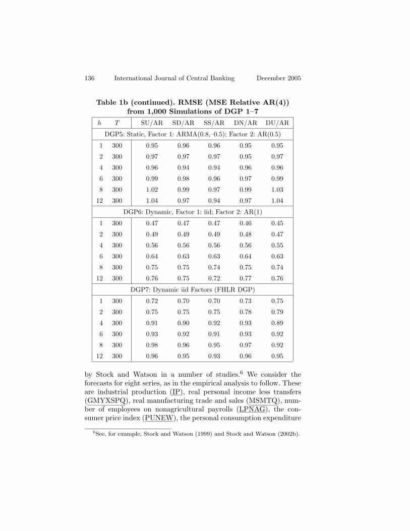
Other results are noteworthy. First, the RMSEs are all belowunity except for DGPs 4 and 5, which are ARMA factors with amoving average component. For these two DGPs, the DN is signifi-cantly better than the other four methods, especially when T = 100.Even with T = 300, the DN continues to be the better methodfor these DGPs. One reason could be because the true lag order ofthe first factor is infinity. In the simulations, we use an AR(3) ap-proximation. As the autoregressive coefficients corresponding to anARMA(.8, –.5) die off slowly, the AR(3) approximation is likely in-adequate. It appears that dynamic misspecification can hamper theproperties of the factor forecasts.

Second, while the differences across methods are small at T =300, they are much larger at T = 100, where the DN and SS areclearly better at long-horizon forecasts. The advantage of the DN atlong horizons is most evident under DGPs 2 and 7, which, inciden-tally, are the DGPs often considered by FHLR. However, the gain issmaller when we mix dynamic with static factors, as in DGP 3. Eventhough DN has smaller errors at long horizons than SU at T = 100,observe also that SS often has smaller errors than DN. This meansthe dynamic factor estimates need not always outperform the staticestimates in forecasting. Attributing differences in forecast errors tothe choice estimator would be misguided.

Taken together, this set of simulation results suggests that thechoice of estimator per se does not seem to make a difference offirst-order importance to the forecast errors. What seems importantis how one combines steps E and F, especially when the time spanof the data is not too long.

5In results not reported, we find that the higher α is, the lower the RMSE,though the relative rankings of the methods do not change.


Table 1a. RMSE (MSE Relative AR(4))from 1,000 Simulations of DGP 1–7

Horizon T Forecasting Methods

h T SU/AR SD/AR SS/AR DN/AR DU/AR

DGP1: Static AR(1) Factors

1 100 0.87 0.86 0.86 0.87 0.86

2 100 0.85 0.85 0.83 0.85 0.85

4 100 0.92 0.89 0.87 0.91 0.92

6 100 0.96 0.94 0.87 0.94 0.96

8 100 0.94 0.91 0.87 0.91 0.94

12 100 0.98 0.92 0.87 0.91 0.98

DGP2: Dynamic AR(1) with α = 0.8

1 100 0.54 0.53 0.53 0.55 0.52

2 100 0.54 0.51 0.51 0.53 0.53

4 100 0.59 0.56 0.55 0.59 0.58

6 100 0.63 0.61 0.59 0.65 0.63

8 100 0.76 0.72 0.67 0.73 0.75

12 100 0.96 0.90 0.84 0.81 0.94

DGP3: Factor 1: Static AR(1); Factor 2: Dynamic AR(1)

1 100 0.62 0.61 0.61 0.64 0.62

2 100 0.53 0.53 0.52 0.57 0.55

4 100 0.55 0.54 0.53 0.62 0.56

6 100 0.73 0.69 0.65 0.72 0.73

8 100 0.84 0.80 0.75 0.81 0.84

12 100 0.87 0.83 0.78 0.82 0.88

DGP4: Static, Factor 1: ARMA(0.8,0.5); Factor 2: AR(0.5)

1 100 0.86 0.79 0.79 0.82 0.85

2 100 0.91 0.79 0.79 0.79 0.90

4 100 0.97 0.86 0.81 0.88 0.96

6 100 1.16 0.98 0.92 0.93 1.15

8 100 1.18 0.97 0.92 0.91 1.17

12 100 1.10 0.96 0.85 0.90 1.10


Table 1a (continued). RMSE (MSE Relative AR(4))from 1,000 Simulations of DGP 1–7

Horizon T Forecasting Methods


DGP5: Static, Factor 1: ARMA(0.8,–0.5); Factor 2: AR(0.5)

1 100 1.12 1.01 1.01 1.00 1.12

2 100 1.08 0.97 0.97 0.98 1.07

4 100 1.09 0.98 0.98 0.98 1.09

6 100 1.19 1.06 1.00 0.99 1.19

8 100 1.14 1.04 0.99 1.00 1.14

12 100 1.24 1.09 1.00 0.96 1.23

DGP6: Dynamic, Factor 1: iid; Factor 2: AR(1)

1 100 0.51 0.50 0.50 0.51 0.51

2 100 0.54 0.52 0.51 0.54 0.52

4 100 0.61 0.59 0.56 0.60 0.60

6 100 0.77 0.73 0.69 0.73 0.76

8 100 0.85 0.81 0.74 0.77 0.84

12 100 0.94 0.87 0.81 0.84 0.95

DGP7: Dynamic iid Factors (FHLR DGP)

1 100 0.70 0.67 0.67 0.68 0.69

2 100 0.86 0.82 0.84 0.82 0.85

4 100 0.99 0.96 0.94 0.95 0.99

6 100 0.96 0.94 0.92 0.91 0.95

8 100 1.04 1.02 0.95 0.98 1.03

12 100 1.04 0.99 0.94 0.94 1.01

5.2 A Calibrated Monte Carlo

The simulations in the previous subsection assume that the id-iosyncratic errors are serially and cross-sectionally uncorrelated tofocus on the factor processes. We now consider a Monte Carlo thatreplicates the error structure of the macroeconomic data set with147 series from 1959:1 to 1998:12. The same data have been used


Table 1b. RMSE (MSE Relative AR(4)) from1,000 Simulations of DGP 1–7


DGP1: Static AR(1) Factors

1 300 0.87 0.87 0.87 0.86 0.87

2 300 0.82 0.81 0.81 0.82 0.82

4 300 0.84 0.82 0.81 0.83 0.84

6 300 0.92 0.92 0.90 0.92 0.92

8 300 0.97 0.97 0.95 0.97 0.96

12 300 0.97 0.97 0.94 0.96 0.97

DGP2: Dynamic AR(1) Factors

1 300 0.52 0.52 0.52 0.52 0.51

2 300 0.46 0.45 0.45 0.45 0.44

4 300 0.61 0.60 0.59 0.59 0.59

6 300 0.70 0.69 0.68 0.67 0.68

8 300 0.72 0.71 0.70 0.71 0.72

12 300 0.81 0.81 0.78 0.79 0.80

DGP3: Factor 1: Static AR(1); Factor 2: Dynamic AR(1)

1 300 0.57 0.56 0.56 0.57 0.56

2 300 0.54 0.53 0.53 0.52 0.52

4 300 0.55 0.54 0.54 0.56 0.55

6 300 0.68 0.67 0.68 0.70 0.70

8 300 0.75 0.74 0.74 0.75 0.75

12 300 0.84 0.84 0.82 0.85 0.86

DGP4: Static, Factor 1: ARMA(0.8,0.5); Factor 2: AR(0.5)

1 300 0.83 0.78 0.78 0.78 0.82

2 300 0.79 0.77 0.77 0.80 0.78

4 300 0.85 0.82 0.82 0.86 0.84

6 300 0.92 0.89 0.86 0.88 0.91

8 300 0.96 0.93 0.91 0.94 0.96

12 300 0.96 0.94 0.92 0.96 0.96


Table 1b (continued). RMSE (MSE Relative AR(4))from 1,000 Simulations of DGP 1–7


DGP5: Static, Factor 1: ARMA(0.8,–0.5); Factor 2: AR(0.5)

1 300 0.95 0.96 0.96 0.95 0.95

2 300 0.97 0.97 0.97 0.95 0.97

4 300 0.96 0.94 0.94 0.96 0.96

6 300 0.99 0.98 0.96 0.97 0.99

8 300 1.02 0.99 0.97 0.99 1.03

12 300 1.04 0.97 0.94 0.97 1.04

DGP6: Dynamic, Factor 1: iid; Factor 2: AR(1)

1 300 0.47 0.47 0.47 0.46 0.45

2 300 0.49 0.49 0.49 0.48 0.47

4 300 0.56 0.56 0.56 0.56 0.55

6 300 0.64 0.63 0.63 0.64 0.63

8 300 0.75 0.75 0.74 0.75 0.74

12 300 0.76 0.75 0.72 0.77 0.76

DGP7: Dynamic iid Factors (FHLR DGP)

1 300 0.72 0.70 0.70 0.73 0.75

2 300 0.75 0.75 0.75 0.78 0.79

4 300 0.91 0.90 0.92 0.93 0.89

6 300 0.93 0.92 0.91 0.93 0.92

8 300 0.98 0.96 0.95 0.97 0.92

12 300 0.96 0.95 0.93 0.96 0.95

by Stock and Watson in a number of studies.6 We consider theforecasts for eight series, as in the empirical analysis to follow. Theseare industrial production (IP), real personal income less transfers(GMYXSPQ), real manufacturing trade and sales (MSMTQ), num-ber of employees on nonagricultural payrolls (LPNAG), the con-sumer price index (PUNEW), the personal consumption expenditure

6See, for example, Stock and Watson (1999) and Stock and Watson (2002b).


deflator (GMDC), the CPI less food and energy (PUXX), and theproducer price index for finished goods (PWFSA).

The calibration exercise aims to preserve the relative importanceof the common and the idiosyncratic errors, the serial and cross-section correlation in the idiosyncratic errors, as well as potentialparameter instability in the data. In the empirical analysis to follow,the first forecast is based on estimation over a sample with 133 obser-vations (corresponding to 1959:3 to 1970:1), while the last estimationsample has 445 observations (corresponding to 1997:1). Recalibrat-ing the model parameters and performing a Monte Carlo at each Twould be extremely time consuming. Instead, starting with T = 133,T is extended every twelve months, a new model is recalibrated, andnew T + h forecasts are obtained. This exercise still takes two weeksto execute.

The calibration consists of estimating r static factors by themethod of principal components at every T , where r is determined asdiscussed below. The estimated common component, χit = λ

′iFt, t =

1, . . . T is then treated as fixed. Data are simulated by adding to χit

new draws of the idiosyncratic errors. More precisely, least-squaresregression of the AR(1) model eit = ρieit−1 + vit yields ρi,T andvit, i = 1, . . . N , noting that if the t-statistic for ρi,T is less than 2in absolute value, we set ρi,T to zero. Resampling v•,t with replace-ment yields a new set of residuals—say, v•,t—which, along with ρi,T ,yields a T by N matrix of idiosyncratic errors that preserve thecross-correlation structure.7 That is to say, if τ ij,T = 1

T

∑Tt=1 vitvjt

is the cross-section covariance over a sample of size T , the simulatederrors vit and vjt will have the same covariance on average. Allowingthe serial and cross-section covariance structure to change over timepermits us to evaluate the forecasts when the data are not covariancestationary. This might be of empirical relevance as macroeconomicdata are known to exhibit substantial parameter instability.

The appendix provides summary statistics on the common andidiosyncratic components, computed at twenty-six values of T atwhich the model is calibrated. The mean of the nonzero ρi,T indicates

7An alternative procedure is to first estimate Ωv = 1T

∑Tt=1 vt v

′t , and then

multiple random draws of N(0,1) errors into the choleski decomposition of Ω. By

construction, the rank of Ωv is N minus the number of factors. The procedurewould require dropping six series from the simulations, since we estimated sixfactors.


that many of the eit are serially correlated, while the mean of τ ij,T in-dicates that some vit pairs are quite strongly cross-correlated. Whileρi,T appears quite stable over time, τ ij,T seems to have fallen overtime on average. The number of series that are serial and cross-correlated has also fallen over the sample. It would be difficult touse simple, parametric models to capture such heterogeneity andparameter instability. The present calibrated Monte Carlo aims toshed light on the factor forecasts in a realistic setting.

The number of factors, the dynamic structure of the factors, andthe dynamic structure of the idiosyncratic errors are now treated asunknown parameters. The BIC is used to jointly determine px, pF ,and r in SU, based on the static principal components. The r usedin SU is also used for SD and SS. The BIC is then used to determineqx, qF , and r in DU, which is based on the generalized principalcomponents. The r used for DU is also used for DN with q fixed to2. The BIC is also used to determine pD

e and pSe , the lag order of the

idiosyncratic errors in SS and SD, as well as pSF and pD

F , the lag orderof the VAR in the factors in SS and SD. Note that these parametersare repeatedly reoptimized because the model is recalibrated eachtime the sample is extended. We fix throughout q to 2, M = H = 20when constructing Γχ(0) and Γe(0). The benchmark forecast is basedon an AR(4).

The results in tables 2a and 2b are averaged over forecasts madeat the twenty-six values of T . On average, the estimation consists of289 observations. Our eight series can be classified into two groups—four nominal and four real. For the four series reported in table 2a,we see that the SU and DU now have significantly smaller RMSEsthan the other methods at long horizons. In fact, the DN loses theedge in long-horizon forecasts that it enjoyed in the simple MonteCarlo experiments. In this calibrated setting, the two unconstrainedforecasts of the real variables tend to outperform the three forecaststhat are based on models with more structure.

For the four series considered in table 2b, a notable result is thatthe factor forecasts yield more modest improvements over the ARforecasts. Only in long-horizon SU and DU forecasts for PUNEWand GMDC did we witness an RMSE below .80. At long horizons,the SD can produce forecasts that are much inferior to the AR. Ofall the methods considered, the SU and DU appear to make largergains over the AR forecasts at every horizon.


Table 2a. RMSE for Calibrated DGP from300 Simulations, Real Variables

Horizon Variable Forecasting Methods

SU/AR SD/AR SS/AR DN/AR DU/AR

1 IP 0.87 0.80 0.80 0.88 0.84

GMYXSPQ 0.75 0.79 0.79 0.84 0.74

MSMTQ 0.83 0.87 0.87 0.87 0.83

LPNAG 0.79 0.71 0.71 0.84 0.79

2 IP 0.73 0.70 0.69 0.81 0.72

GMYXSPQ 0.72 0.76 0.76 0.83 0.70

MSMTQ 0.77 0.80 0.80 0.83 0.75

LPNAG 0.83 0.70 0.69 0.86 0.83

4 IP 0.64 0.58 0.64 0.86 0.67

GMYXSPQ 0.69 0.75 0.75 0.90 0.69

MSMTQ 0.69 0.74 0.75 0.85 0.70

LPNAG 0.67 0.63 0.65 0.74 0.69

6 IP 0.56 0.58 0.59 0.80 0.62

GMYXSPQ 0.63 0.71 0.73 0.83 0.60

MSMTQ 0.64 0.70 0.73 0.81 0.64

LPNAG 0.57 0.69 0.65 0.69 0.59

8 IP 0.63 0.68 0.69 0.81 0.68

GMYXSPQ 0.67 0.76 0.80 0.82 0.60

MSMTQ 0.64 0.70 0.77 0.81 0.64

LPNAG 0.64 0.81 0.71 0.69 0.62

12 IP 0.65 0.77 0.75 0.80 0.68

GMYXSPQ 0.64 0.77 0.85 0.81 0.61

MSMTQ 0.63 0.71 0.79 0.81 0.66

LPNAG 0.61 0.88 0.76 0.73 0.61


Table 2b. RMSE for Calibrated DGP from300 Simulations, Nominal Variables



1 PUNEW 0.91 0.93 0.93 0.93 0.91

GMDC 0.88 0.90 0.90 0.90 0.89

PUXX 0.97 0.98 0.98 0.97 0.97

PWFSA 0.94 0.95 0.95 0.95 0.95

2 PUNEW 0.91 0.92 0.92 0.95 0.92

GMDC 0.87 0.93 0.93 0.92 0.89

PUXX 0.96 0.97 0.97 0.97 0.97

PWFSA 0.94 0.95 0.95 0.96 0.94

4 PUNEW 0.84 0.88 0.88 0.92 0.86

GMDC 0.78 0.94 0.94 0.88 0.80

PUXX 0.95 0.97 0.97 0.96 0.96

PWFSA 0.91 0.93 0.93 0.94 0.92

6 PUNEW 0.83 0.89 0.88 0.91 0.85

GMDC 0.76 0.97 0.96 0.85 0.78

PUXX 0.94 0.99 0.98 0.96 0.96

PWFSA 0.91 0.94 0.94 0.94 0.92

8 PUNEW 0.86 0.93 0.91 0.92 0.88

GMDC 0.77 1.03 0.99 0.85 0.80

PUXX 0.95 1.03 1.01 0.95 0.96

PWFSA 0.94 0.97 0.96 0.95 0.94

12 PUNEW 0.87 1.04 0.96 0.92 0.90

GMDC 0.76 1.13 1.04 0.83 0.83

PUXX 0.94 1.10 1.04 0.95 0.97

PWFSA 0.94 1.02 0.97 0.95 0.95


Comparing DN with DU in tables 2a and 2b, the DU generallyhas significantly smaller errors than the DN. Comparing SU with SDand SS, the SU tends to be the better of the three. These differencesunderscore the point that step F can generate important differencesin forecast errors. As noted earlier, even when the factors and theidiosyncratic errors are observed, how much forecast improvementthe factors can provide depends on λi and the difference betweenthe dynamics of the factors and the errors. While no one methodsystematically outperforms the others for the real series at shorthorizons (i.e., h = 1, 2, 4), the SU always has the smallest errorfor forecasting the nominal series, and the SU and DU are best forforecasting the real series at longer horizons.

An overview of the results in tables 1 and 2 is as follows. Forsimple data-generating processes such as those in table 1, the SUor DU cannot be supported as the best method. However, once weconsider more complex error structures such as the ones encounteredin the data, the two unrestricted forecasts become noticeably betterthan all other methods. Unlike the SS and SD, the SU and DU donot specify the dynamics of Ft. As well, many auxiliary parametersneed to be chosen in order to estimate the dynamic factors. Simpleimplementation and leaving the forecasting equation with the flexi-bility to adapt to the complex properties data may explain why theunconstrained forecasts perform much better when the errors areheterogeneous in many dimensions. It remains to consider whetherthe various forecasting methods perform in the data as they do insimulations.

6. Application to Eight Series

Results for various diffusion index forecasts are available in the lit-erature. As is clear from the discussion above, there are many waysto construct forecasts using the factor estimates. FHLR reported re-sults for static forecasts, but they implemented what would havebeen SN in our notation, not the SU that Stock and Watson used.On the other hand, Stock and Watson evaluated the DU forecasts,8

but these are not the same as the DN that FHLR proposed. As well,the results are reported for different forecast horizons, and using

8See for example, Stock and Watson (2004a) and Forni et al. (2005).


different criteria. Here, we provide an objective comparison of thevarious methods, making clear the role of steps E and F.

We apply the five methods to eight series: IP, GMYXSPQ,MSMTQ, LPNAG, PUNEW, GMDC, PUXX, and PWFSA. Thegoal is to forecast the growth rates of the real variables and infla-tion rates h periods hence. For xit, we consider a balanced panel ofN=147 monthly series available from 1959:1 to 1998:12. FollowingStock and Watson (2002b), the data are standardized and trans-formed to achieve stationarity where necessary before the factorsare estimated. The logarithms of the four real variables are assumedto be I(1), while the logarithms of the four prices are assumed tobe I(2).

The forecasting exercise begins with data from 1959:3–1970:1. Anh-period-ahead forecast is formed by using values of the regressorsat 1970:1 to give yh

1970:1+h. The sample is updated by one month,the factors and the forecasting equation are both reestimated, andan h-month forecast for 1971:2 is formed. The final forecast is madefor 1998:12 in 1998:12–h. Recursive AR(p) forecasts are likewise con-structed. Several auxiliary parameters must again be chosen. As inthe calibrated Monte Carlo, we determine qx, r, and qF jointly usingthe BIC. Given this r, we then use the BIC to determine pD

F , pSF , pD

e ,pS

e . For the dynamic factors, we again set M to 20 and fix q to 2.Table 3 reports the MSE relative to the optimal AR(p) model,

where p is also chosen by the BIC. Overall, the improvements ofthe factor forecasts over the autoregressive forecasts for the infla-tion series (table 3b) are modest.9 However, the SU and DU arenoticeably better than the three methods that maintain a factorstructure in the forecasting equation. Interestingly, the SU did notdo as well in forecasting GMYXSPQ and MSMTQ in the calibratedsimulations, and they also do not perform favorably in the empiricalexercise.

For the real series (table 3a), all methods are quite similar ath = 1. However, there are nontrivial differences at other horizons.The RMSEs are all below unity at all forecast horizons, and theygenerally fall with h. Observe that (i) SS and SU tend to outperformSD, (ii) DU outperforms DN in twenty-three of twenty-four cases,

9Results in Inoue and Kilian (2003) suggest that for data with a weak factorstructure, factor forecasts might be less effective.


Table 3a. RMSE for Real Variables, 1970:1998



1 IP 0.83 0.86 0.86 0.85 0.82

GMYXSPQ 0.81 0.84 0.84 0.90 0.87

MSMTQ 0.87 0.88 0.88 0.90 0.88

LPNAG 0.83 0.97 0.97 0.89 0.85

2 IP 0.73 0.79 0.77 0.80 0.73

GMYXSPQ 0.77 0.78 0.76 0.82 0.75

MSMTQ 0.83 0.84 0.84 0.87 0.82

LPNAG 0.74 0.88 0.86 0.79 0.78

4 IP 0.66 0.70 0.67 0.73 0.78

GMYXSPQ 0.76 0.71 0.69 0.77 0.67

MSMTQ 0.76 0.75 0.74 0.83 0.75

LPNAG 0.64 0.87 0.82 0.71 0.66

6 IP 0.55 0.67 0.63 0.74 0.64

GMYXSPQ 0.69 0.72 0.69 0.75 0.65

MSMTQ 0.76 0.74 0.73 0.83 0.72

LPNAG 0.60 0.74 0.71 0.69 0.59

8 IP 0.56 0.71 0.64 0.75 0.58

GMYXSPQ 0.74 0.73 0.70 0.75 0.66

MSMTQ 0.80 0.78 0.76 0.86 0.75

LPNAG 0.59 0.73 0.68 0.70 0.60

12 IP 0.49 0.60 0.53 0.71 0.55

GMYXSPQ 0.70 0.74 0.72 0.76 0.63

MSMTQ 0.80 0.75 0.74 0.88 0.78

LPNAG 0.49 0.60 0.57 0.64 0.54

and (iii) all of the twenty-four best forecasts are generated by SUor DU, which do not impose a factor or a dynamic structure onthe forecasts. Looking across series and forecast horizon, SU has the


Table 3b. RMSE for Nominal Variables, 1970:1998



1 PUNEW 0.96 0.99 0.99 1.00 0.97

GMDC 0.95 0.99 0.99 0.99 0.95

PUXX 0.93 1.00 1.00 1.00 0.93

PWFSA 0.94 0.98 0.98 0.98 0.94

2 PUNEW 0.86 0.89 0.89 0.91 0.85

GMDC 0.93 0.96 0.96 0.95 0.91

PUXX 0.85 0.98 0.98 0.93 0.84

PWFSA 0.91 0.97 0.97 0.98 0.91

4 PUNEW 0.68 0.77 0.77 0.84 0.66

GMDC 0.84 0.92 0.92 0.91 0.85

PUXX 0.80 0.98 0.98 0.92 0.80

PWFSA 0.80 0.87 0.87 0.86 0.84

6 PUNEW 0.65 1.42 1.42 0.95 0.65

GMDC 0.83 0.96 0.95 0.96 0.87

PUXX 0.79 0.98 0.98 0.93 0.81

PWFSA 0.75 0.90 0.90 0.85 0.77

8 PUNEW 0.65 1.71 1.67 1.01 0.67

GMDC 0.82 1.31 1.30 0.98 0.90

PUXX 0.81 0.97 0.97 0.99 0.81

PWFSA 0.75 0.96 0.95 0.87 0.76

12 PUNEW 0.55 1.53 1.51 0.89 0.62

GMDC 0.73 1.29 1.27 0.94 0.82

PUXX 0.77 0.99 0.98 0.94 0.78

PWFSA 0.71 0.92 0.90 0.83 0.71

smallest error in thirteen cases. The DU is best in eleven cases. Theseresults are broadly similar to our calibrated Monte Carlo.

Result (i) is consistent with Marcellino, Stock, and Watson (2004)that sequential forecasts tend to outperform direct forecasts. Re-sults (i) and (ii) reinforce the point that step F can yield important


differences in the forecasting errors. Result (iii) points to the ro-bustness of the unconstrained forecasts. The choice of static versusdynamic factor estimates is less important. This is at odds withthe perception that a fully specified dynamic factor model (the DN)should yield better forecasts. We offer several explanations. The firstis simply that the static factor model is a better characterization ofthe data. The dynamic estimates would then unnecessarily smooththe spectrum over different frequencies and suffer efficiency loss. Sec-ond, the DN has only been shown to be more efficient in counter-factually simple examples. Whether the dynamic estimator remainsefficient when, for example, s > 0 for only a subset of the factors isunclear. Furthermore, it should be kept in mind the object of inter-est is forecast of a series, not precise estimation of the factors or thecommon component per se. That the Stock-Watson unconstrainedmethod produces better forecasts does not mean it will produce amore precise estimate of the common component.

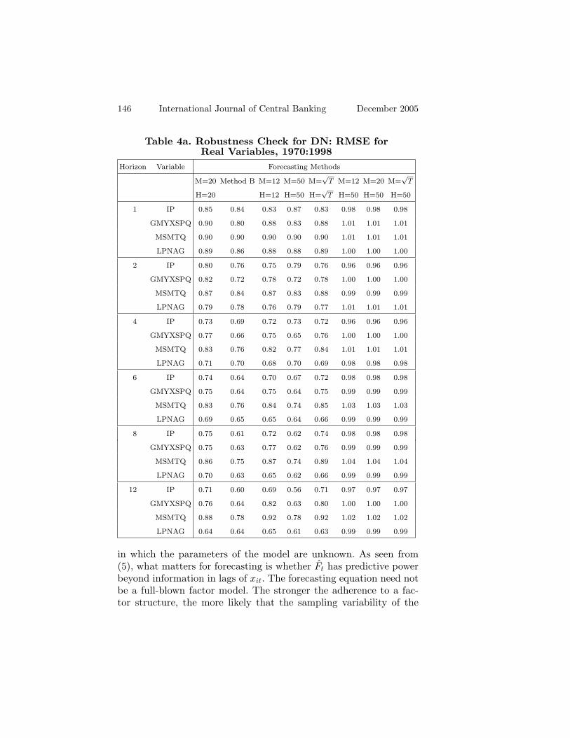
Third, our results might reflect the fact that we have not tunedthe parameters to maximize the efficiency of the dynamic estimator.To get a sense of this issue, table 4 reports additional results for theDN. Instead of selecting s as described above, we first compute theout-of-sample forecasts for every configuration of the parameters forthe full sample of 456 observations. The optimal s is the one thatminimizes the time-averaged MSE. This method, which we refer to asmethod B in table 4, thus fixes s over the entire sample period.10 Theresults in table 4 suggest that method B produces better forecastsfor the real series, but not the nominal series. We next consider thesensitivity of the DN to the choice of M and H. In addition to thebase case of M = H = 20, table 4 also provides results for M = H =12, 50 and

√T , as well as alternative values of M holding H fixed

at 50. The RMSEs are generally smaller with H = M = 50. Overall,table 4 suggests that the dynamic factor forecasts can indeed beimproved with better choices of the auxiliary parameters. However,it is far less clear that the improvements will be large enough to beatthe SU or the DU, at least for the series considered.

Taking the empirical and simulation results together, we findthat the SU and DU perform better in practice and in simulations

10This method was considered in the working paper version of Forni et al.(2005). Note that in contrast to other methods, this is not, strictly speaking, anout-of-sample exercise since the auxiliary parameters are selected on the basis ofthe out-of-sample performance.


Table 4a. Robustness Check for DN: RMSE forReal Variables, 1970:1998


M=20 Method B M=12 M=50 M=√

T M=12 M=20 M=√

T

H=20 H=12 H=50 H=√

T H=50 H=50 H=50

1 IP 0.85 0.84 0.83 0.87 0.83 0.98 0.98 0.98

GMYXSPQ 0.90 0.80 0.88 0.83 0.88 1.01 1.01 1.01

MSMTQ 0.90 0.90 0.90 0.90 0.90 1.01 1.01 1.01

LPNAG 0.89 0.86 0.88 0.88 0.89 1.00 1.00 1.00

2 IP 0.80 0.76 0.75 0.79 0.76 0.96 0.96 0.96

GMYXSPQ 0.82 0.72 0.78 0.72 0.78 1.00 1.00 1.00

MSMTQ 0.87 0.84 0.87 0.83 0.88 0.99 0.99 0.99

LPNAG 0.79 0.78 0.76 0.79 0.77 1.01 1.01 1.01

4 IP 0.73 0.69 0.72 0.73 0.72 0.96 0.96 0.96

GMYXSPQ 0.77 0.66 0.75 0.65 0.76 1.00 1.00 1.00

MSMTQ 0.83 0.76 0.82 0.77 0.84 1.01 1.01 1.01

LPNAG 0.71 0.70 0.68 0.70 0.69 0.98 0.98 0.98

6 IP 0.74 0.64 0.70 0.67 0.72 0.98 0.98 0.98

GMYXSPQ 0.75 0.64 0.75 0.64 0.75 0.99 0.99 0.99

MSMTQ 0.83 0.76 0.84 0.74 0.85 1.03 1.03 1.03

LPNAG 0.69 0.65 0.65 0.64 0.66 0.99 0.99 0.99

8 IP 0.75 0.61 0.72 0.62 0.74 0.98 0.98 0.98

GMYXSPQ 0.75 0.63 0.77 0.62 0.76 0.99 0.99 0.99

MSMTQ 0.86 0.75 0.87 0.74 0.89 1.04 1.04 1.04

LPNAG 0.70 0.63 0.65 0.62 0.66 0.99 0.99 0.99

12 IP 0.71 0.60 0.69 0.56 0.71 0.97 0.97 0.97

GMYXSPQ 0.76 0.64 0.82 0.63 0.80 1.00 1.00 1.00

MSMTQ 0.88 0.78 0.92 0.78 0.92 1.02 1.02 1.02

LPNAG 0.64 0.64 0.65 0.61 0.63 0.99 0.99 0.99

in which the parameters of the model are unknown. As seen from(5), what matters for forecasting is whether Ft has predictive powerbeyond information in lags of xit. The forecasting equation need notbe a full-blown factor model. The stronger the adherence to a fac-tor structure, the more likely that the sampling variability of the


Table 4b. Robustness Check for DN: RMSE forNominal Variables, 1970:1998


M=20 Method B M=12 M=50 M=√

T M=12 M=20 M=√

T

H=20 H=12 H=50 H=√

T H=50 H=50 H=50

1 PUNEW 1.00 0.96 1.00 1.01 1.00 1.00 1.00 0.97

GMDC 0.99 1.00 0.99 0.99 0.99 0.99 0.99 0.95

PUXX 1.00 0.96 1.00 1.00 1.00 1.00 1.00 0.93

PWFSA 0.98 0.98 0.98 0.98 0.98 0.98 0.98 0.94

2 PUNEW 0.91 0.93 0.91 0.91 0.90 0.98 0.98 0.85

GMDC 0.95 0.99 0.96 0.96 0.96 0.98 0.98 0.91

PUXX 0.93 0.95 0.92 0.94 0.91 1.02 1.02 0.82

PWFSA 0.98 0.97 0.97 0.97 0.97 0.98 0.98 0.93

4 PUNEW 0.84 0.91 0.82 0.83 0.83 0.98 0.98 0.69

GMDC 0.91 0.97 0.92 0.90 0.92 0.99 0.99 0.83

PUXX 0.92 0.96 0.90 0.93 0.89 1.11 1.11 0.77

PWFSA 0.86 0.94 0.85 0.87 0.86 0.92 0.92 0.84

6 PUNEW 0.95 0.88 0.95 0.87 0.94 0.99 0.99 0.68

GMDC 0.96 0.96 0.94 0.90 0.95 0.98 0.98 0.85

PUXX 0.93 0.94 0.97 0.95 0.95 1.16 1.16 0.81

PWFSA 0.85 0.95 0.84 0.85 0.84 0.92 0.92 0.79

8 PUNEW 1.01 0.85 0.99 0.97 0.97 0.99 0.99 0.72

GMDC 0.98 0.96 0.91 0.92 0.94 1.00 1.00 0.88

PUXX 0.99 0.92 0.95 0.96 0.97 1.15 1.15 0.81

PWFSA 0.87 0.98 0.85 0.88 0.85 0.95 0.95 0.80

12 PUNEW 0.89 0.79 0.82 0.90 0.83 0.97 0.97 0.63

GMDC 0.94 0.92 0.87 0.89 0.86 1.00 1.00 0.80

PUXX 0.94 0.93 0.94 0.94 0.94 1.11 1.11 0.76

PWFSA 0.83 0.91 0.80 0.83 0.79 0.95 0.95 0.79

factor estimates will enter the forecasts. When the parameters of thedata-generating process are also unknown and/or are unstable, mis-specification of the dynamics can magnify the sampling variability ofthe factor estimates. The favorable properties of the unconstrained


forecasts are likely due to the minimal factor structure imposed onthe forecasting equation and the simplicity in its implementation.

Finally, given that the SU and DU have rather similar finite sam-ple properties, a comment on SU versus DU is in order. Of the two,the SU is much easier to implement. The SU only requires the user todetermine r, px, and pF by applying the BIC to the forecasting equa-tion. Estimation of the dynamic factors necessitates choosing variousparameters for which we have no guide. It should also be mentionedthat in practice and following FHLR, the dynamic factors are con-structed as the generalized principal components of Σx − diag(Γe(0)),not Γχ(0) = Σx − Γe(0) as theory suggests. A symmetric treatmentwould have the static factors estimated as the generalized principalcomponents of Σx −diag(Ω). Boivin and Ng (2004) suggest that thiscould further improve the SU. Such a method is not implementedbecause Ω is not a diagonal matrix in an approximate factor model.While the methods work in practice, more work is required at thetheoretical level to justify its use.

7. Conclusion

In this paper, we seek to better understand how factors estimatedfrom a large panel of data can be used in forecasting exercises. Inprinciple, how the factors are estimated and how the forecasts areformed can both affect the mean-squared forecast error. We find thatfor simple error structure, differences across methods exist, especiallywhen T is small, but the differences are not so strong as to immedi-ately favor a particular method. When more complicated but realisticerror structures are considered, the unconstrained method proposedby Stock and Watson works systematically better. The method alsobehaves noticeably better in the empirical analysis. This methodsimply augments estimates of the factors to an autoregressive fore-casting equation. We attribute its performance to not imposing atight factor structure and having to choose a small number of aux-iliary parameters. This leaves the forecasting equation with moreflexibility to adapt to the data. The fully specified dynamic factorforecasts have the potential for improvements, but more needs to belearned about how to adapt the auxiliary parameters to the data onhand. Finally, the static factors are easier to construct than dynamicfactors, and are favored on practical grounds.


Appendix. Descriptive Statistics of the Idiosyncratic Termin the Calibrated DGP

Sample Size |ρi , T | maxj |τ i j | 1N

∑j|τ i j | %|τ i j | > 0.2 R2

i

1−N ∗/N Mean Std Mean Std Mean Std Mean Std

133 0.21 0.43 0.19 0.71 0.22 0.12 0.03 0.15 0.36 0.28

145 0.23 0.42 0.18 0.71 0.22 0.12 0.04 0.16 0.36 0.27

157 0.18 0.41 0.19 0.71 0.22 0.11 0.03 0.14 0.41 0.27

169 0.16 0.39 0.18 0.69 0.23 0.11 0.03 0.15 0.46 0.28

181 0.21 0.39 0.19 0.66 0.23 0.11 0.03 0.13 0.55 0.26

193 0.15 0.39 0.20 0.67 0.23 0.11 0.03 0.12 0.52 0.27

205 0.15 0.39 0.20 0.67 0.23 0.11 0.03 0.12 0.52 0.27

217 0.13 0.39 0.21 0.67 0.23 0.10 0.03 0.11 0.52 0.27

229 0.17 0.40 0.21 0.67 0.23 0.10 0.03 0.11 0.52 0.27

241 0.17 0.39 0.21 0.67 0.23 0.11 0.03 0.13 0.53 0.26

253 0.18 0.38 0.19 0.67 0.23 0.11 0.03 0.12 0.53 0.26

265 0.20 0.38 0.20 0.64 0.23 0.10 0.03 0.11 0.60 0.26

277 0.17 0.37 0.20 0.63 0.23 0.10 0.03 0.10 0.60 0.26

289 0.17 0.38 0.20 0.63 0.23 0.10 0.02 0.10 0.60 0.26

301 0.14 0.38 0.20 0.63 0.23 0.10 0.02 0.10 0.60 0.26

313 0.12 0.37 0.20 0.63 0.22 0.10 0.02 0.10 0.60 0.26

325 0.14 0.38 0.20 0.63 0.22 0.10 0.02 0.10 0.59 0.26

337 0.12 0.38 0.21 0.63 0.22 0.09 0.02 0.10 0.59 0.26

349 0.16 0.38 0.21 0.60 0.22 0.09 0.02 0.10 0.64 0.24

361 0.15 0.39 0.21 0.61 0.22 0.09 0.02 0.10 0.64 0.24

373 0.12 0.38 0.21 0.63 0.22 0.09 0.02 0.10 0.59 0.26

385 0.16 0.38 0.21 0.61 0.22 0.09 0.03 0.10 0.64 0.24

397 0.15 0.38 0.20 0.59 0.22 0.09 0.02 0.09 0.66 0.24

409 0.14 0.38 0.20 0.59 0.22 0.09 0.02 0.09 0.66 0.24

421 0.15 0.39 0.20 0.59 0.22 0.09 0.02 0.09 0.65 0.24

433 0.14 0.39 0.20 0.59 0.22 0.09 0.02 0.08 0.65 0.24

445 0.14 0.39 0.21 0.59 0.22 0.09 0.02 0.08 0.65 0.24

Mean 0.16 0.39 0.20 0.64 0.23 0.10 0.03 0.11 0.56 0.26

Std 0.02 0.01 0.01 0.04 0.00 0.01 0.00 0.02 0.09 0.01

Note: The mean and standard deviation reported in the columns are overtaken over i.

N ∗ is the number of ρi that are statistically different from zero at the two-tailed 5 percent

level.


References

Anderson, Theodore W., and H. Rubin. 1956. “Statistical Infer-ence in Factor Analysis.” In Proceedings of the Third BerkeleySymposium on Mathematical Statistics and Probability, Vol. V,ed. J. Neyman, 114–50. Berkeley: University of California Press.

Bai, Jushan. 2003. “Inferential Theory for Factor Models of LargeDimensions.” Econometrica 71 (1): 135–72.

Bai, Jushan, and Serena Ng. 2002. “Determining the Number of Fac-tors in Approximate Factor Models.” Econometrica 70 (1): 191–221.

Boivin, Jean, and Serena Ng. 2004. “Are More Data Always Betterfor Factor Analysis?” Forthcoming in Journal of Econometrics.

Brillinger, David R. 1981. Time Series: Data Analysis and Theory.San Francisco: Wiley.

Chamberlain, Gary, and Michael Rothschild. 1983. “Arbitrage, Fac-tor Structure and Mean-Variance Analysis on Large Asset Mar-kets.” Econometrica 51:1305–24.

Connor, Gregory, and Robert A. Korajzcyk. 1986. “PerformanceMeasurement with the Arbitrage Pricing Theory: A New Frame-work for Analysis.” Journal of Financial Economics 15 (3):373–94.

Forni, Mario, Marc Hallin, Marco Lippi, and Lucrezia Reichlin.2000. “The Generalized Dynamic Factor Model: Identificationand Estimation.” Review of Economics and Statistics 82 (4):540–54.

———. 2001. “Coincident and Leading Indicators for the EuroArea.” Economic Journal 111 (471): C82–5.

———. 2004. “The Generalized Factor Model: Consistency andRates.” Journal of Econometrics 119 (2): 231–55.

———. 2005. “The Generalized Dynamic Factor Model: One-SidedEstimation and Forecasting.” Journal of the American StatisticalAssociation 100 (471): 830–40.

Forni, Mario, and Lucrezia Reichlin. 2001. “Federal Policies and Lo-cal Economies: Europe and the US.” European Economic Review45 (1): 109–34.

Grenouilleau, Daniel. 2004. “A Sorted Leading Indicators Dynamic(SLID) Factor Model for Short-Run Euro-Area DGP Forecast-ing.” European Commission Economic Papers 219.


Inoue, Atsushi, and Lutz Kilian. 2003. “Bagging Time Series Mod-els.” Unpublished Manuscript, North Carolina University.

Kapetanios, George, and Massimiliano Marcellino. 2002. “A Com-parison of Estimation Methods for Dynamic Factor Models ofLarge Dimensions.” Draft, Bocconi University.

Kitchen, John, and Ralph M. Monaco. 2003. “Real-Time Forecastingin Practice: The U.S. Treasury Staff’s Real-Time GDP ForecastSystem.” Business Economics (October): 10–19.

Marcellino, Massimiliano, James Stock, and Mark Watson. 2004. “AComparison of Direct and Iterated AR Methods for ForecastingMacroeconomic Time Series h-steps Ahead.” Mimeo, PrincetonUniversity.

Stock, James H., and Mark W. Watson. 1999. “Forecasting Infla-tion.” Journal of Monetary Economics 44 (2): 293–335.

———. 2002a. “Forecasting Using Principal Components from aLarge Number of Predictors.” Journal of the American Statis-tical Association 97 (460): 1167–79.

———. 2002b. “Macroeconomic Forecasting Using Diffusion In-dexes.” Journal of Business and Economic Statistics 20 (2):147–62.

———. 2004a. “An Empirical Comparison of Methods for Forecast-ing Using Many Predictors.” Mimeo, Princeton University.

———. 2004b. “Forecasting with Many Predictors.” In The Hand-book of Economic Forecasting, ed. G. Elliott. Elsevier Science.

Stock, James H., Mark W. Watson, and Massimiliano Marcellino.2003. “Macroeconomic Forecasting in the Euro Area: CountrySpecific versus Area-Wide Information.” European Economic Re-view 47 (1): 1–18.

understanding and comparing factor-based forecastssn2294/pub/ijcb05.pdf · understanding and...

Documents