UNDERGRADUATE STUDENTS’ ATTITUDES TOWARD STATISTICS

IN AN INTRODUCTORY STATISTICS CLASS

by

KRISTI LYNN CLARK

(Under the Direction of Jennifer J. Kaplan)

ABSTRACT

Students’ attitudes influence their performance, beliefs, and behavior in classes,

especially in terms of motivation and achievement. It is, therefore, important that we monitor and

attempt to improve the attitudes of statistics students toward statistics in the classroom. Four

instruments designed to assess attitudes toward statistics have reasonable reliability and validity

evidence: Statistics Attitude Survey, Attitude toward Statistics, and the two versions of the

Survey of Attitudes toward Statistics. These instruments are compared and then UGA students’

responses to the SATS-28 Pre and their achievement in STAT 2000 are examined. Our research

goal is to see whether the students’ pre-course SATS-28 scores are associated with the students’

achievement. We consider the relationship between the SATS-28 Pre score and the total test

points. Additionally, we analyze qualitative data that indicate why students have positive or

negative attitudes toward statistics. We conclude with suggestions for improving attitudes among

STAT 2000 students.

INDEX WORDS: Statistics Education; Attitudes Toward Statistics; Introductory Statistics;

Validity; Reliability

UNDERGRADUATE STUDENTS’ ATTITUDES TOWARD STATISTICS

IN AN INTRODUCTORY STATISTICS CLASS

by

KRISTI LYNN CLARK

B.S., Clayton State University, 2010

A Thesis Submitted to the Graduate Faculty of The University of Georgia in Partial Fulfillment

of the Requirements for the Degree

MASTER OF SCIENCE

ATHENS, GEORGIA

2013

© 2013

Kristi Lynn Clark

All Rights Reserved

UNDERGRADUATE STUDENTS’ ATTITUDES TOWARD STATISTICS

IN AN INTRODUCTORY STATISTICS CLASS

by

KRISTI LYNN CLARK

Major Professor: Jennifer J. Kaplan

Committee: Jaxk Reeves

Kim Gilbert

Electronic Version Approved:

Maureen Grasso

Dean of the Graduate School

The University of Georgia

December 2013

iv

ACKNOWLEDGEMENTS

First I would like to thank God for His blessings; I cannot do anything with His help. I

would also like to express my thanks to my parents and brother for all their encouragement and

support. I would like to express my appreciation to Dr. Kaplan for all her time and assistance. I

would like to thank Dr. Reeves and Dr. Gilbert for taking to time to serve on my committee as

well as the members of my thesis group: Elizabeth Amick, Greg Jansen, Kyle Jennings, Alex

Lyford, Adam Molnar, and Allison Moore for their time and help. I would also like to thank Mr.

Morse and Dr. Love-Myers for all their help throughout my thesis.

v

TABLE OF CONTENTS

Page

ACKNOWLEDGEMENTS ........................................................................................................... iv

LIST OF TABLES ........................................................................................................................ vii

LIST OF FIGURES ..................................................................................................................... viii

CHAPTER

1 INTRODUCTION .........................................................................................................1

2 LITERATURE REVIEW ..............................................................................................3

2.1 Defining Affective Constructs and Attitudes ....................................................3

2.2 Relationship between Attitudes and Learning ...................................................3

2.3 Evaluating Measurement Scales ........................................................................6

2.4 Measuring Attitudes Toward Statistics ............................................................11

2.5 Previous Findings with Respect to Attitudes and Student Learning ...............19

3 DATA COLLECTION AND METHODS .................................................................29

3.1 Setting .............................................................................................................29

3.2 Subjects ............................................................................................................31

3.3 Instruments .......................................................................................................31

3.4 Analysis............................................................................................................32

4 RESULTS ....................................................................................................................36

4.1 Comparison of the Three Sub-groups of Students ..........................................36

4.2 Comparison between UGA STAT 2000 and the Population ...........................38

vi

4.3 Modeling the Relationships between Attitude, Effort, and Achievement .......44

4.4 Summer 2013 Data ..........................................................................................52

5 CONCLUSION ............................................................................................................55

REFERENCES ..............................................................................................................................60

APPENDICES

A R-Code .........................................................................................................................64

A.1 To compare the sub-groups using T-tests for Fall 2012 and Summer 2013

Data .......................................................................................................................64

A.2 To create the histograms, scatterplots, and boxplots for students with

complete data .........................................................................................................64

A.3 Model Selection without the observation with missing Age observation .......65

A.4 Model Selection with all observations with complete data ............................67

A.5 Cronbach’s Alpha ...........................................................................................68

vii

LIST OF TABLES

Page

Table 3.1: Conversion of Variable: Course Grade to New Variable: Course GPA .......................33

Table 3.2: Description of Variables used in the Analysis ..............................................................35

Table 4.1: Summary Statistics for UGA STAT 2000 students ......................................................36

Table 4.2: T-test summaries ...........................................................................................................37

Table 4.3: Summary Statistics for SATS Pre for UGA students who complete the course ..........41

Table 4.4: Z-test summaries for students who complete the course ..............................................42

Table 4.5: Summary Statistics for SATS Pre for UGA students who did not complete the

course .................................................................................................................................43

Table 4.6: Z-test summaries for UGA students who did not complete the course ........................43

Table 4.7: Correlations for UGA STAT 2000 students with complete data ..................................47

Table 4.8: Regression Model .........................................................................................................50

Table 4.9: Themes to Students’ Attitudes ......................................................................................53

Table 4.10: Two-Way Table for Attitude and Perceived Usefulness ............................................54

viii

LIST OF FIGURES

Page

Figure 4.1: Histograms of SATS sub-scores for STAT 2000 students with complete data ..........40

Figure 4.2: Histogram of Test Total on UGA STAT 2000 students with complete data ..............45

Figure 4.3: Histograms of Homework Completed and Labs Completed on UGA STAT 2000

students with completed data .............................................................................................46

Figure 4.4: Scatterplots of SATS sub-scores for STAT 2000 students with complete data ..........47

Figure 4.5: Boxplots of STAT 2000 course data with moderate to high correlations for students

with complete data .............................................................................................................49

Figure 4.6: The Residual Plot of the model ...................................................................................51

1

CHAPTER 1

INTRODUCTION

Students’ attitudes have an influence on their performance in a class and how they will

develop statistical skills and ability to apply their knowledge outside the class (Gal, Ginsburg,

and Schau, 1997). A student’s attitudes “influence and are influenced by” his/her beliefs (Gal,

Ginsburg, and Schau, 1997, pg. 41). Attitudes also affect the student’s behavior, especially in

terms of motivation and achievement (Dweck, 2002). Since most undergraduate students are

required to take only one statistics course to graduate, student’s attitudes toward statistics are

considered very important. After the course, the students with negative attitudes will probably

never use statistics again in their personal or professional lives (Ramirez, Schau & Emmioglu,

2012).

At the University of Georgia, the STAT 2000 course satisfies the General Education Core

Curriculum requirement for quantitative reasoning and is required for many majors on campus.

Many students who may have no prior or future experience with statistics take STAT 2000 every

semester. Given the results of the research on the importance of attitudes, which will be

discussed in more detail in Chapter 2, it is important that we monitor the attitudes of our STAT

2000 students toward statistics in the classroom and attempt to improve their attitudes.

In order to do this, we must have a measure of student attitudes toward statistics. We will

consider the four most widely used instruments designed to measure students’ attitudes toward

statistics: Statistics Attitude Survey (SAS), Attitude Toward Statistics Scale (ATS), and the two

versions of the Survey of Attitudes Toward Statistics (SATS-28 and SATS-36). We will describe

2

how and why instruments were created and the constructs they are designed to measure. We will

also look at the validity and reliability claims of each survey and discuss why we chose to use the

SATS-28 as the basis for this work. We will also provide a brief description of previous findings

about student attitudes toward statistics.

The original research, presented in Chapters 3-5, is based on student responses to the

SATS-28 given at the beginning of the semester as well as student achievement in STAT 2000,

measured by number of assignments completed and points earned during the semester. Our

research goal is to see whether the students’ pre-course SATS-28 scores are associated with the

students’ achievement. In this thesis, we will look to see if there is a relationship between

the SATS-28 Pre score and the total test points earned in class. In addition, analysis of qualitative

data which describe why students have positive or negative attitudes will be presented. The work

concludes with suggestions for the UGA Statistics Department’s STAT 2000 Coordinator that

will help improve the attitudes toward statistics of the students enrolled in the STAT 2000

course.

3

CHAPTER 2

LITERATURE REVIEW

2.1 Defining Affective Constructs and Attitudes

The term affective is defined as “relating to, arising from, or influencing feelings or

emotions” (Merriam-Webster.com, 2013). Affective constructs include the sub-classes of

attitudes, emotions, dispositions, and motivations. Within each of these sub-classes, there exist

more narrow constructs, for example, anxiety, curiosity, desire to learn, effort, expectations,

interest, participation, perceived value, persistence, self-efficacy, and many more (Pearl,

Garfield, delMas, Groth, Kaplan, McGowan, and Lee, 2012). Attitude is described as being

relatively stable, including strong feelings that have developed over time through repeated

emotional responses that can be positive or negative (Gal, Ginsburg, and Schau, 1997). The

work presented in this paper focuses on student attitudes as they relate to statistics and the

learning of statistics.

2.2 Relationship between Attitudes and Learning

A student’s attitudes “influence and are influenced by” his/her beliefs (Gal, Ginsburg,

and Schau, 1997, pg. 41). According to Gal, Ginsburg and Schau (1997) students’ attitudes

toward and beliefs about statistics can either help or hurt their learning of statistics. The authors

also claim that attitudes influence how students will develop statistical skills and abilities to

apply their knowledge outside the classroom. Three specific ways in which attitudes toward

4

statistics may manifest in and out of the classroom are in considerations of process, outcome, and

access (Gal, Ginsburg, and Schau, 1997).

Process considerations are the role that attitudes play in influencing the learning process.

For example, if an instructor desires to have a problem-solving environment in the classroom,

s/he should build a supportive atmosphere where the students feel safe to explore, speculate,

hypothesize, and experiment with different statistical tools and methods. Students should also

feel comfortable with temporary confusion and the uncertainty inherent in statistical situations,

and should believe in their own ability to navigate through the decisions and problems in order to

finish any project. In order to help the students develop the mind-sets necessary for this type of

classroom to function well, teachers must assess and monitor their students’ attitudes (Gal,

Ginsburg, and Schau, 1997).

Outcome considerations are the role that attitudes have in influencing the students’

statistical behavior after their class. For example, students should emerge from their statistics

classes with willingness and interest to use statistics in their professional and/or personal lives

(Gal, Ginsburg, and Schau, 1997). Access considerations are the role that attitudes play in

influencing the students’ desire to continue to learning statistics. After student has taken the

required first statistics class, a positive student attitude in this dimension would be demonstrated

by the student enrolling in a second course in statistics, while a negative attitude by choosing not

to take another course (Gal, Ginsburg, and Schau, 1997).

A person’s behavior is affected by his/her beliefs, especially in terms of motivation and

achievement (Dweck, 2002). A motivated person is eager or prompted toward an end. Students

can be motivated to complete their homework out of interest or desire for their parents’ or

teacher’s approval (Ryan and Deci, 2000). The student’s belief about his/her intelligence affects

5

his/her motivation. There are two theories of intelligence that a student may believe: intelligence

is a fixed trait that cannot be developed or intelligence is a malleable trait that can be improved.

When students believe their intelligence is fixed, they want to appear smart, and as if they

already know the material. Among other behaviors, such students will not ask for help. These

students with a belief in fixed intelligence will chose to miss valuable learning opportunities in

order to continue looking smart and not risk making errors. To these students, failure and

outward signs of effort devoted to learning signifies low intelligence. After encountering

difficulty in a subject, such students will expend less effort because they believe that working

hard is useless and a sign of being unintelligent. They actually chose failure over effort in order

to preserve their belief of ability. If they fail a subject by not trying hard, they are still able to

say that they could have done well if they had wanted to. Students with fixed intelligence belief

will risk their future so that they won’t feel or look bad in the present (Dweck, 2002).

On the other hand, when students believe that their intelligence is malleable, they are

willing to learn new things, even if they risk failure. Their goal is to master the subject over time,

not to outdo other students. To them, mistakes happen to everybody and simply show what

needs to be done to improve. Mistakes encourage them to spend more effort on the task, or to

change their strategy for learning. Effort to them does not mean they are stupid, but rather that

they are getting the chance to improve their ability to the fullest (Dweck, 2002).

Dweck studied how different types of praise affect the different views of intelligence held

by students. She found that when students were given intelligence-praise, they were more likely

to develop a fixed view of their intelligence than were students given effort-praise (2002). In

addition, she has reported that students’ theories of intelligence are able to be changed, even for

undergraduate students (Dweck, 2002). Since the students’ theories of intelligence can be

6

changed, it would benefit statistics teaching and learning if research could suggest a way to help

students move from the mind-set of ‘I cannot do statistics’ to ‘I can do statistics if I am willing to

try hard’.

Furthermore, by applying other disciplines’ theories and findings to statistics education, it

has been suggested that students who have negative attitudes when leaving their statistics courses

will probably never use it again. This provides more evidence that it is extremely important that

introductory statistics teachers try to influence their students’ attitudes, since the majority of the

students are required to take only one course (Schau and Emmioglu, 2012).

2.3 Evaluating Measurement Scales

In order to monitor the level of students’ attitudes toward statistics and to determine

whether students leaving a class have more positive attitudes, we must have a way to measure

such attitudes (Pearl, et al., 2012). As with any assessment or measurement instrument, a test of

attitudes must be a valid and reliable measure of the construct. In other words, the test user must

be able to justify the inferences drawn by the test score by having a rational reason for using the

test score for the intended purpose and for selecting a particular test (Crocker and Algina, 1986).

Reliability and validity are two prerequisites for the justification. In this section, we provide an

overview of reliability and validity from a measurement perspective. These ideas are used to

evaluate the available instruments to measure students’ attitudes toward statistics.

2.3.1 Reliability

Reliability is the consistency of test scores across replications of a testing procedure.

There are two types of errors of measurement, which can reduce the reliability of the test scores:

7

systematic and random. Systematic errors will constantly affect the examinee’s score because of

a characteristic that has nothing to do with the construct being measured. A systematic error will

be repeated every time the examinee is given the tests using the same instruments. An example

of systematic error would be a student who always marks ‘neutral’ instead of choosing to either

agree or disagree with a statement. Random errors of measurement affect the examinee’s test

score by chance. They will not be repeated exactly on future tests. Random errors can have a

positive or negative effect on the examinee’s score. One example of a random error is guessing,

because in different administrations of the same test, a student may choose different answers.

Systematic and random errors of measurement are both concerns for score interpretation,

affecting the usefulness of the test scores. Random errors can also affect the consistency of the

test scores (Crocker and Algina, 1986).

There are two types of reliability: internal and external. Internal reliability/consistency is

the degree of consistency among item response on a single survey measuring the same dimension

(Nolan, Beran, and Hecker, 2012). While there are several procedures to calculate internal

reliability, in this paper we will discuss only Cronbach’s alpha, also known as coefficient alpha.

Cronbach’s alpha is calculated using the formula: , where k = the number of

items, = the variance of the item i, and = the total test variance (Crocker and Algina, 1986).

Cronbach’s alpha, α, can be between 0 and 1. The more internally consistent the test is, the

closer α is to 1. External reliability/stability is the consistency of the scores between times of

administration (test-retest reliability) and/or raters (inter-rater reliability) (Nolan, Beran, &

Hecker, 2012).

8

2.3.2 Validity

The reliability of a measurement is not enough to justify validity of the scores, but the

measurement cannot be valid without being reliable (Nolan, Beran, & Hecker, 2012). “Validity

is an overall evaluative judgment of the degree to which empirical evidence and theoretical

rationales support the adequacy and appropriateness of interpretations and actions on the basis of

test scores or other modes of assessment” (Messick, 1995, pg.741). In order for the meaning or

interpretation of the test and/or its implications for action to be useful, the test must be valid.

Validity evidence should be collected constantly to ensure that the instruments continue to keep

up with the setting and contexts (Messick, 1995). Validation is an “evaluative summary of both

the evidence for actual – as well as potential – consequences of score interpretation and use”

(Messick, 1995, pg. 742).

There are three major types of validity evidence: content, criterion-related, and construct.

Content validation is the study of the relationship between the test items and the performance

domain or construct of special interest (Crocker and Algina, 1986). When the test user wants to

collect evidence to support an inference from the test score of an examinee to a larger domain of

interest, he/she will use content validation. Content validation takes place after the initial

development of the test. Minimally, four steps must be completed for content validation: (1)

defining the domain of interest, (2) selecting a group of experts to examine and judge the test

items in terms of performance in the domain, (3) having a structured framework to match the test

items to the domain, and (4) gathering and summarizing the data from step 3. Issues to consider

within content validity are whether the objectives represent the domain, whether it is meaningful

for examinees of different ethnic or cultural backgrounds, and whether the content validation is

relevant to the judgment of the item performance data (Crocker and Algina, 1986).

9

“Criterion-related validation is the study of the relationship between test scores and a

practical performance criterion” (Crocker and Algina, 1986, pg. 238). When the test user wants

to collect evidence to support an inference from the test score of an examinee to a performance

criterion that cannot be directly measured for a real and practical behavior variable, he/she uses

criterion-related validation. The steps for criterion-related validation are to identify and measure

a suitable criterion behavior, to identify a sample of examinees that is appropriate and

representative of future examinees, to administer the test to examinees and record each score, to

obtain each examinee’s performance measurement on criterion when criterion data is available,

and, finally, to determine the test scores and criterion performance relationship strength. The two

types of criterion-related validation are predictive validity and concurrent validity. Predictive

validity measures how the test score will predict future criterion measurement. Concurrent

validity measures how the test score relates to the current criterion measurement. Difficulties that

occur with criterion-related validation are criterion identification and contamination, inadequate

sample sizes, variance limitations, and a predictor or criterion measurement’s lack of reliability.

The validity coefficient is the correlation coefficient between the test score and criterion score.

The validity coefficient is typically used to assess the results of the criterion-related validation

(Crocker and Algina, 1986).

Construct validation is the study of the relationship between test scores and a behavior

domain (Crocker and Algina, 1986). When the test user wants to collect evidence to support an

inference from the test score of an examinee to performance groups under a psychological

construct, he/she will use construct validation. The first step for determining construct validation

is to create hypotheses about how the examinees “who differ on the construct are expected to

differ on demographic characteristics, performance criteria, or measures of other construct whose

10

relationship to performance criteria has already been validated” (Crocker and Algina, 1986, pg.

230). Next, choose or create an instrument that measures the items that represent evident

behaviors of the construct. The third step is to gather empirical data to be able to test

hypothesized relationships. Then, determine whether the data are consistent with the hypotheses,

and consider and attempt to eliminate rival theories and/or alternative explanations that can

explain the observed findings. Construct validation is a gamble, because if the validation study

cannot confirm the hypotheses, the test developer cannot determine whether the critical flaw is in

theoretical construct, the test that measures the construct, or both (Crocker and Algina, 1986).

Since construct validation is applicable for the majority of test types and intended test

score uses, the distinction between the three major types of validation is somewhat artificial

(Crocker and Algina, 1986). Messick unified the concept of validation by combining the

considerations of three major types of validation into a construct framework. He noted that there

are six aspects of construct validation: content, consequential, external, generalizability,

structural, and substantive (Messick, 1995). The definition of content validity was not changed

from the definition above. Consequential validity refers to the score interpretation’s value and

implications and the actual and potential consequences of test use (Messick, 1995). External

validity is a measure of how the survey performs compared to external measures of the same or a

related construct. For external validity, we will look at three correlations patterns: convergent,

discriminant, and predictive (Nolan, Beran, & Hecker, 2012). Convergent validity coefficients

are the correlations between the test scores and other similar measurements of the same

construct. There should be a strong relationship between these two measurements. Discriminant

validity coefficients are the correlations for different constructs for the same test or the

correlations for different constructs with different measurements. Ideally, the discriminant

11

validity coefficients will display a weak relationship and will be lower than the convergent

validity coefficients or the Cronbach’s alpha (Crocker and Algina, 1986). Predictive validity

measures whether there is a reasonably strong relationship between the survey and criterion

variables, such as grades, for example (Nolan, Beran, & Hecker, 2012). Generalizability validity

considers the score traits, quality, and interpretations that are generalized to and across

population groups, settings, and tasks (Messick, 1995). Structural validity examines whether the

survey’s scales, components, and items are reflected by the intended dimensionality of the

construct interpretation (Nolan, Beran, & Hecker, 2012). A substantive validity refers to the

strength of the theoretical basis for interpreting survey scores (Nolan, Beran, & Hecker, 2012).

Demonstrating evidence for all six aspects of construct validation is not required, as long as one

has a good argument and evidence to justify the interpretation and usage of the instrument

(Messick, 1995). Due to lack of evidence, generalizability validity and consequential validity

will not be examined for any of the instruments examined in this thesis.

2.4 Measuring Attitudes Toward Statistics

While recent surveys of the literature (Nolan, Beran, & Hecker, 2012; Ramirez, Schau &

Emmioglu, 2012) report 22 instruments designed to assess attitudes toward statistics, only four

of the instruments have been shown to have reasonable reliability and validity evidence, under

the assumptions of classical test theory (Pearl, et al., 2012). The four instruments, the Statistics

Attitude Survey (SAS), the Attitude Toward Statistics Scale (ATS), and two versions of the

Survey of Attitudes Toward Statistics (SATS-28 and SATS-36), are described in this section.

12

2.4.1 Statistics Attitude Survey (SAS)

Statistics Attitude Survey (SAS) was created by Roberts and Bilderback (1980) in order

to improve the prediction of students’ achievement in statistics classes using an affective scale

(Gal and Ginsburg, 1994). The authors claim SAS has one global attitude component, measured

by 33 questions that cover the supposed usefulness of statistics, personal ability to solve

statistical problems, beliefs about statistics, and affective reactions to statistics. Each question

has a Likert-type scale with five possible responses ranging from strongly agree to strongly

disagree (Ramirez, Schau & Emmioglu, 2012). The wording of the questions varies between

positive or negative, with 16 negative items. More positive attitudes toward statistics are

signified by higher scores (Cashin and Elmore, 2005). Robert and Bilderbeck in 1980 reported

Cronbach’s alpha of α=0.94 for SAS (Cashin and Elmore, 2005), indicating that the SAS has a

high degree of reliability. The SAS was developed without input from students and teachers

(Ramirez, Schau & Emmioglu, 2012), but the main argument against using SAS is that many of

the items assess students’ knowledge about statistics, not their attitudes (Gal and Ginsburg,

1994).

Nolan, Beran, and Hecker (2012), examined the validity and reliability claims of SAS.

They looked at four aspects of validation: content, external, structural, and substantive for SAS.

Content validation for SAS states that the items are appraised as a single dimension, and that it is

based on Dutton’s mathematics content domain and on the perceptions of students of their

competence and statistics’ usefulness. External validation was demonstrated for three parts:

convergent, discriminant, and predictive. Convergent validity was verified by high positive

correlations with both of the ATS components and the total ATS score and moderate positive

correlations with the SATS-28 components. Discriminant validity showed weak and non-

13

significant relationships between the SAS scores and students’ attitude toward calculators.

Predictive validity was investigated using correlations between SAS scores and academic

performance: the highest was 0.54. There was no record of substantive validation. Structural

validation was shown by Principal Components Factor Analysis with ATS components (these

components are discussed more fully in the next section). The reported range for Cronbach’s

alpha associated with SAS is from 0.92 to 0.95 for the pre-course, post-course, and single

administration for all the studies that Nolan, Beran, and Hecker (2012) examined in their paper.

The measures of content validation for the SAS seem acceptable, but there is no evidence

of substantive validation for the SAS. It does have good external validation with convergent,

discriminant, and predictive validity. Nolan, Beran, and Hecker (2012) stated one of the many

studies they examined could not confirm the one factor of SAS for structural validation. Even

though the SAS has the highest Cronbach’s alpha range than the other three instruments, SAS is

not the strongest of the available attitude measurements.

2.4.2 Attitudes Toward Statistics (ATS)

Wise developed Attitudes Toward Statistics Scale (ATS) in 1985 (Ramirez, Schau &

Emmioglu, 2012). ATS has 29 questions that cover two components: Field (20 questions) and

Course (9 questions). Field measures students’ attitudes toward statistics in their field of study.

Course measures students’ attitudes toward their current statistics course. Like the SAS, each

question on the ATS has a Likert-type scale with five possible responses, ranging from strongly

disagree to strongly agree. The wording of the questions varies between positive or negative.

ATS also was developed without input from students and is not based on theory (Ramirez, Schau

& Emmioglu, 2012).

14

Wise (1985) provided reliability and validity evidence for the ATS. Wise started with 40

questions, but after testing the questions for content validity, he retained 29. There were 92

students in his study. The Cronbach’s alpha was 0.92 for Field and 0.90 for Course. Test-retest

reliability coefficients were 0.82 for Field and 0.91 for Course. Wise allowed two weeks

between testing. He also analyzed factorial validity that showed that the two rotated factors were

identifiable as corresponding to Field and Course. The presence of two common factors

accounted for 49% of the total variance. Lastly, he examined the criterion-related validity by

considering the relationship between the ATS score and the student’s course grade. The student’s

grade had a significant relationship with Course, but not Field. Wise claimed that this shows

each of his components, Field and Course, were measuring different types of attitudes (Wise,

1985).

Nolan, Beran, and Hecker (2012) examined the validity and reliability evidence for ATS.

Content validation for ATS was done by having the items for Field and Course approved by five

statistics instructors. Again, external validation was shown in three parts: convergent,

discriminant, and predictive. For the convergent validity evidence, both of the ATS components

and the total ATS score had high positive correlations with SAS. ATS Course and SATS-28

Value are moderately positive correlated, as are ATS Course and SATS-28 Difficulty. ATS

Course and SATS-28 Affect are highly correlated, as well as ATS Course and SATS-28

Cognitive Competence. ATS Field was highly correlated with SATS-28 Value. There was no

discriminant validity evidence for the ATS. Predictive validity shows weak correlations between

ATS and academic performance: the highest was 0.47 for post test. There was no record of

substantive validation for ATS. Structural validation was shown in three ways: Principal-axis

Factor Analysis with SATS-28 items, Principal Components Factor Analysis with ATS

15

components, and principal factor solution. The reported Cronbach’s alpha range is 0.83 to 0.96

for Field, 0.77 to 0.92 for Course, and 0.89 to 0.94 for Total ATS score for all the studies that

Nolan, Beran, and Hecker (2012) examined in their paper. The reliability evidence for the ATS is

based on the Cronbach’s alpha and test-retest reliability coefficients. Content validation was

tested using teachers. It provided no evidence of substantive validation. The structural validation

has supported the evidence that ATS is a two factor model. External validation had good

convergent evidence with the SAS and SATS and predictive evidence, but there was no

discriminant evidence. Thus, ATS is not the strongest of the available attitude measurements.

2.4.3 Survey of Attitudes Toward Statistics (SATS)

Survey of Attitudes Toward Statistics (SATS) was created by Candace Schau in 1992.

The original survey, SATS-28, has 28 questions that cover four attitude components: affect,

cognitive competence, value, and difficulty. In 1995, the SATS-28 was revised to include two

more attitude components: interest and effort. This version of SATS is called SATS-36. Each

edition of SATS has a pre-course and post-course version. The main difference between the pre-

course and post-course versions is in the grammatical tense used in the statements. SATS-28 and

SATS-36 also contains three additional global attitude questions in the pre-course and post-

course version, and the SATS-36 post-course version has an additional global attitude question

on global effort.

The components measured by the SATS are defined as follows (Schau, 2003): the affect

component (6 questions) assesses the students’ feelings regarding statistics. The cognitive

competence component (6 questions) evaluates students’ attitude concerning their intellectual

knowledge and skills when applied to statistics. The value component (9 questions) assesses the

16

students’ belief that statistics can be useful, relevant, and worthy in their personal and

professional life. The difficulty component (7 questions) evaluates the students’ attitudes about

the difficulty of statistics. The interest component (4 questions) determines the students’ interest

in statistics. The effort component (4 questions) measures the amount of work the student is

willing to do to learn statistics.

Each question has a Likert-type scale with seven possible responses that range from 1:

strongly disagree to 7: strongly agree with a midpoint 4: neither disagree nor agree. Students are

advised to chose 4 if they have no opinion about the given statement. For Difficulty, the higher

scores indicate that the students believe that statistics will be easy, while lower scores indicate

that the students believe statistics will be hard. The wording of the questions varies between

positive or negative. The scores are determined by reversing the number for the negatively

worded questions, then adding the responses in each component, and finally dividing by the

number of questions in each component (Schau, 2003).

Ramirez, Schau and Emmioglu (2012) stated that there was an eight step quantitative and

qualitative development process used to create both versions of SATS. To create the SATS,

Schau first inspected the previous statistical surveys and obtained a written description of

introductory statistics students’ attitudes. Then she used a group of instructors and students to

sort words and phrases describing students’ statistics attitudes into components. SATS went

through pilot testing, and afterwards, a revision of items. The validation of the four-component

internal structure of SATS-28 had been confirmed by using Confirmatory Factor Analysis. Based

on the SATS-28’s relationships or lack of relationship with other measures’ scores, the validation

of component scores was confirmed. Schau added two additional attitude components to create

17

SATS-36. Using Confirmatory Factor Analysis, the validation of the six-component internal

structure of SATS-36 was verified.

Schau, Dauphinee, & Del Vecchio (1995) stated that concurrent validity of SATS-28 is

supported by significant correlations with ATS. SATS-28 was validated for Content and

construct validity through item analysis. There was confirmation of the dimensionality of SATS

using Confirmatory Factor Analysis. The researchers reported the Cronbach’s alpha range for

each component: Affect: 0.81 to 0.85, Cognitive Competence: 0.77 to 0.83, Value: 0.80 to 0.85,

and Difficulty: 0.64 to 0.77 from several different studies (Schau, Dauphinee, & Del Vecchio,

1995). Nolan, Beran, and Hecker (2012) examined the validity and reliability claims of SATS-

28. Content validation for SATS-28 states that the items were developed with input from

undergraduate and graduate students and instructors. Substantive validation evidence shows that

SATS-28 is similar to expectancy value, social cognition, and goal theories of learning. Evidence

for structural validation was shown using parceled Confirmatory Factor Analysis, which verified

that SATS-28 measures four dimensions. Nevertheless, parallel exploratory factor analysis with

SATS-28 and Principal-axis Factor Analysis with ATS items shows two dimensions by

combining Affect, Cognitive Competence and Difficulty into one component. Only the four-factor

model had an acceptable goodness-of-fit chi-square result when compared to the one-, two-, and

three-factor models using parceled Confirmatory Factor Analysis. External validation was

showed in three parts: convergent, discriminant, and predictive. For the convergent validity

evidence, SATS-28 components had moderate positive correlations with SAS. SATS-28 Value &

ATS Course and SATS-28 Difficulty & ATS Course are moderately positive correlated. SATS-

28 Affect & ATS Course, SATS-28 Cognitive Competence & ATS Course, SATS-28 Value &

ATS Field were all highly correlated. The discriminant validity evidence for the SATS-28 shows

18

moderate relationships between SATS-28 Affect and Cognitive Competence and attitudes toward

mathematics. Predictive validity shows weak correlations between SATS-28 and academic

performance, but using structural equation modeling and regression showed that between 2% and

21% of the variance in students’ achievement were accounted by SATS-28. For the pre-course,

post-course, and single administration, the Cronbach’s alpha reported ranges for SATS

components were Affect: 0.74 to 0.89, Cognitive Competence: 0.71 to 0.86, Value: 0.63 to 0.90

and Difficulty: 0.51 to 0.76 for all the studies that Nolan, Beran, and Hecker (2012) examined in

their paper.

Nolan, Beran, and Hecker (2012) also considered the validity and reliability claims of

SATS-36. Content validation was the development of two additional components. For external

validity evidence, there is no convergent and discriminant validation evidence for SATS-36. The

predictive validity shows weak correlations between SATS-36 and academic performance, but

using structural equation modeling showed that 10% of the variance in students’ achievement

was accounted for by SATS-36. Substantive validation shows that the two additional

components, Interest and Effort, increased with the expectancy-value theory of learning.

Structural validation evidence was shown using two different types of Confirmatory Factor

Analysis: parceled and unparceled. The analyses confirmed that SATS-36 measures six

dimensions. One study using unparceled Confirmatory Factor Analysis indicted there could be a

four-factor model that combined Affect, Cognitive Competence and Difficulty into one

component. The reported Cronbach’s alpha range for the pre-course, post-course, and single

administration for Interest was 0.80 to 0.88 and for Effort was 0.71 to 0.85 for all the studies that

Nolan, Beran, and Hecker (2012) examined in their paper.

19

SATS-28 was the only instrument that had evidence for content, external, substantive,

and structural validity: all four types of validation. SATS-28 has been most thoroughly

developed when compared to SAS and ATS for content and substantive validation. The revision

of SATS-28 to SATS-36 would seem to increase both the content and substantive validity, but

neither the initial development nor validation has been published to establish this assertion.

SATS-28 and SATS-36 have inconsistent evidence for structural validation. Different types of

factor analyses state that SATS-28 could be either a two- or four-factor model; the SATS-36

could be a four-factor model or six-factor model by combining Affect, Cognitive Competence,

and Difficulty in one component. This is possibly due to the high correlation between the

components, although there has been additional evidence confirming the dimensions of the

SATS. External validation had good convergent and predictive evidence. There was weak

discriminant evidence with good correlation with attitude toward mathematics, which might

show that SATS-28 is measuring a different construct. SATS-36 had good predictive validity

evidence for external, but no evidence for convergent and discriminant (Nolan, Beran, and

Hecker, 2012). SATS-28 and SATS-36 had mostly good Cronbach’s alphas with Difficulty

having the lowest. Based on the evidence, SATS-28 seems to be strongest of the available

measures of attitude. SATS-36 might be, once the initial development or validation has been

published to prove this conclusion.

2.5 Previous Findings with Respect to Attitudes and Student Learning

Schau and Emmioglu (2012) used the SATS-36 to examine the attitudes toward statistics

of introductory statistics students. They were interested in the students’ attitudes at the

beginning and end of the course, as well as why the students’ attitudes changed during the

20

semester. Schau and Emmioglu obtained their data from United States institutions ranging small

private and public four-year colleges to large research universities that award advanced degrees.

They selected students from introductory statistics service courses that were taught in statistics

and mathematics departments. In their results, the researchers reported that for three of the

components, Affect, Cognitive Competence, and Difficulty, the means showed only slight

improvement from pre-course to post-course, with differences of less than 0.15 on a scale from 1

to 7:. The mean decrease for the components of Value, Interest, and Effort from pre-course to

post-course were -0.32, -0.50, and -0.48 respectively. The students, on average, had a neutral

attitude on the difficulty component of the SATS for the pre-course and post-course surveys.

Since the students’ attitude on the effort component was very high from the pre-course, it was

acceptable to the researchers that the effort component had decreased at the post-course because

students may have realized that they overestimated the amount of effort they would spend on

statistics. However, Schau and Emmioglu (2012) did not discover the improvements they hoped

to see in the other four components. Instead they found no change for Affect and Cognitive

Competence and decreases for Interest and Value.

Griffith, Adams, Gu, Hart, and Nichols-Whitehead (2012) used a mixed methods

approach to determine whether the major of the students had a relationship with the students’

attitudes. The participants were enrolled in an undergraduate statistics course. The participants’

majors were business, criminal justice, and psychology. Griffith, Adams, Gu, Hart, and Nichols-

Whitehead designed their own survey with two questions. One question asked whether their

attitude toward statistics was positive or negative. The students did not have the option to state

that their attitudes were neutral. They were forced to choose either positive or negative. The

second question asked for the reason for their attitudes. The researchers used a chi-square test

21

which detected a relationship between attitude toward statistics and major. Then they used a

Bonferroni correction to study the difference between majors. The evidence suggested that

business majors had more positive attitudes than criminal justice and psychology majors. The

difference between business and criminal justice was significant although the difference between

the business and psychology students was not significant.

Vanhoof, Sotos, Onghena, Verschaffel, Van Dooren, & Van den Noortgate (2006) did a

study using ATS to investigate students’ attitudes toward statistics and the relationship between

those attitudes and short-term and long-term statistics exam results. The participants are Flemish

students who took an introductory undergraduate statistics course and were enrolled in the

Department of Educational Sciences. The researchers administered a Dutch translation of ATS

scale in the beginning of the first and second year statistics courses. The researchers recorded the

students’ statistics exam results and dissertation grades to use as measures of statistics

performance. The statistics exam results are from the statistics course the students must take

during their first three years. During the fourth and fifth years the students do not take a specific

course, but the dissertation includes methodology and statistics. For the first year and second

year statistics courses, there is a statistically significant positive correlation between the ATS

Course and the exam results. Only for the first year statistics course is the difference between the

correlations of Course versus Field statistically significant for the second administration. For the

third year statistics exam results and the fifth year dissertation, the researchers found no

statistically significant correlation with the ATS score. They also found no statistically

significant correlation between the short-term and long-term general exams results and the ATS.

Cashin and Elmore (2005) did a study on the construct validity of SATS-28 scores and

their relationship with ATS and SAS scores. The study was done at a large Midwestern

22

university using students enrolled in two statistics classes. One of the classes was an upper-level

undergraduate course that had both undergraduate and graduate students. The other class had

only graduate students. The students voluntarily took three attitude surveys, SATS-28, ATS, and

SAS, during the first two weeks of the semester and again in the last two weeks. Students also

completed a biographical information sheet at the beginning of the semester. The course grades

were obtained and standardized to have a mean of 500 and standard deviation of 100. This study

found no evidence of a difference in attitudes toward statistics or statistics course achievement

with respect to gender. SATS-28 Value and ATS Field component score had the highest

correlation values. SATS-28 Affect and Cognitive Competence component scores had the highest

correlation values with SAS total score and ATS Course component scores. SATS-28 Difficulty

had positive correlation with all the components of SAS and ATS, but the correlation was lower

than the other components of SATS-28. This seems to indicate that SATS-28 Difficulty

component measures an attitude trait that was not measured by the SAS or ATS. Cashin and

Elmore (2005) also used a factor analysis on the SATS-28, SAS, and ATS items. The factor

analyses indicate that SATS-28 might have only two dimensions, contradicting the SATS-28

developers, who claim the test has four dimensions. It was expected that SATS-28 Value and

ATS Field would be equivalent because both measure the attitude about the value of statistics.

Similarly, SATS-28 Affect and Cognitive Competence and ATS Course would be matched

because all three components measure the attitude toward performance in the class. SATS-28

Difficulty was believed to be different from ATS components and the other SATS components

because it was designed to measure a new construct. Cashin and Elmore (2005), however, did

not find this to be the case.

23

Ramirez, Schau, and Emmioglu (2012) developed a Model of Students’ Attitudes Toward

Statistics (SATS-M), which includes three main constructs that influence course outcomes in

statistics. The three constructs are: students’ characteristics (age, gender, demographic

characteristics), previous achievement related experiences (previous statistics and mathematics

courses and grade point average), and students’ attitudes (measured by the SATS-36). Ramirez,

Schau, and Emmioglu (2012) assume that students’ attitudes include all six components of

SATS-36. The resulting model shows that at the beginning of a course only the student

characteristics influence student attitudes. The course outcome, however, is influenced by both

student characteristics and attitudes. After the students complete the course, the course outcome

also influences the next related course, along with student characteristics and attitude.

This model was developed using Eccles’ Expectancy Value Theory (EVT) as the

framework. Eccles’ EVT assumes that students’ beliefs about their ability to do a task and about

the value of the task are associated. Also, these beliefs should predict the students’ achievement-

related outcomes. These related outcomes in statistics are enrollment and completion of statistics

classes, the desire to work hard to learn and accomplish, and the desire to use statistics in life.

Eccles and his colleagues believe that value, which they called Subjective Task Value, is a super-

construct that cannot be measured, but its sub-components can be measured. These sub-

components include Interest, Affect, Value, and Effort form SATS. Eccles’ (2012) EVT also

include the constructs of Difficulty and Cognitive Competence. Three other theories that support

SATS-M are Self-determination Theory (measures Affect, Interest, Value, and Cognitive

Competence), Self-efficacy Theory (measures Cognitive Competence), and Achievement Goal

Theory (measures Value and Effort).

24

Schau (2003b) reports seven results about students’ attitudes when data are collected with

SATS-28. Students’ attitudes were more negative when asked orally, rather than in SATS written

form. Also, students believe that their attitudes could be attributed to their previous achievement

and instructors. On average, a student’s SATS score reflects positive attitudes in Cognitive

Competence and Value, a neutral attitude in Affect, and a negative attitude in Difficulty. There

was a large difference between each component’s mean scores. Mean attitudes vary with the

different course section at the beginning and end of semester. For the students who completed

both pre-course and post-course, there was difference of 0.90 for Affect, 0.69 for Cognitive

Competence, 0.73 for Value, and 0.65 for Difficulty, all on a scale from 1 to 7, between the

lowest and highest section means. By controlling for gender as well as ethnic groups (Whites and

Hispanics), it was found that there were similar mean pre-course attitudes component scores. For

the post-course, males and Whites have slightly better attitudes than females and Hispanics on

some components. Each component’s mean scores decreased from the beginning of class to the

end. Only the mean score of one component, Value, decreased more than 0.2 points; it decreased

by 0.4 points on a scale from 1 to 7. Finally, the student’s attitudes and achievement were

positively related.

Schau (2008) raises six common categories of errors that have been made in the

conducting of SATS research

1. Design and Measurement Issues: includes researchers revising or dropping items

and/or components, giving the SATS once, but stating an attitude change, using small

sample sizes, and not being able to match up pre-course and post-course scores.

25

2. Participant Issues: includes omitting the number and the percentage of participating

students and/or investigating only the matching pre-course and post-course responses

and omitting the students who only took one test (pre-course or post-course).

3. Scoring Issues: includes ignoring score distributions, not inspecting the quality of the

attitude component score by examining the internal consistency, miscalculating the

mean score of the component by including missing scores as ‘zero’, and calculating a

mean total SATS score because this allows components with more questions to have

more influence in the students’ scores.

4. Analysis Issues: includes the researcher grouping dissimilar students, such as

combining undergraduate and graduate students, and using gain scores when a linear

model using pre-course score as a predictor would be more appropriate because of the

shared variance between pre-course scores and gain scores.

5. Results Issues: includes the researchers not reporting the central tendency and

variability, or failing to highlight the statistical significance.

6. Context Reporting Issues: includes the researcher not reporting the course and

instructor characteristics, institution type, instructional methods, and student

demographics.

Emmioglu and Capa-Aydin (2012) did a meta-analysis of studies that used the SATS-28.

They searched for articles about attitudes toward statistics. They only kept 17 articles in their

study because these articles included participants that were post-secondary education students,

reported the Pearson correlation coefficient between attitudes and achievements, used SATS-28,

and reported at least one of the four SATS-28 components and the post-course attitudes. The

majority of these studies reported a positive relationship between achievement and each of the

26

SATS attitude components. The correlation between achievement and Affect, as well as the

correlation between achievement and Cognitive Competence, was higher than achievement with

Value or Difficulty. Emmioglu and Capa-Aydin observed that region influenced the relationship

between achievement and attitudes.

Josh Beamer (2013), using similar methodology to Schau and Emmioglu (2012),

analyzed individual student scores, instead of section mean. He compared and contrasted the

students’ attitudes with two types of curriculum across five institutions. The first curriculum was

the traditional approach that focuses on individual concepts and statistical inference at the end of

course. The second curriculum was the Randomization-Based curriculum that focuses on

statistics inference, technology, and working thorough all introductory statistics material instead

of one concept at a time during the whole semester. Before comparing the different curricula, he

compared the results for students using both curricula with the national data. For the combined

groups, there was a positive difference between pre- and post-test for Affect, Cognitive

Competence, and Difficulty. Value, Interest, and Effort had a negative difference. Effort had the

highest difference with -0.71. He then created six models to predict the difference between the

pre-course and post-course scores for each component. Curriculum was included in the models

as a predictor, along with gender, confidence, study time, teaching curriculum, and current GPA.

For the categorical variable associated with curriculum, Randomization-Based curriculum that

was taught multiple times, was the reference group. The other two levels of this variable were

Traditional curriculum and Randomization-Based curriculum taught for the first or second time.

While the significance of the variables was different for each model, gender and current GPA

were never significant. Confidence was a significant predictor in the Affect and Cognitive

Competence models. Study time was significant at α=0.1 for the Affect, Value, Difficulty,

27

Interest, and Effort models. Traditional curriculum was a significant negative predictor at α=0.1

for the Affect, Cognitive Competence, Difficulty and Effort models. The indicator variable for

Randomization Based curriculum taught the first or second time was a significant negative

predictor at α=0.1 for the Value model. Randomization Based curriculum taught the first or

second time was a significant positive predictor at α=0.1 for the Interest and Effort models. This

study concludes that more positive attitudes seem to be influenced by Randomization-Based

curriculum taught multiple times compared to the Traditional Curriculum or Randomization-

Based curriculum taught the first or second time.

The examination of the previous work on students’ attitudes toward statistics presented in

this chapter has guided the research presented in the subsequent chapters. Some researchers have

looked at the difference between pre-course and post-course scores of SATS. Researchers have

also looked at the relationship between attitude several variables: the students’ major, the

students’ gender, the students’ achievement (short-term mostly), and different types of

curriculum. This previous research provides additional evidence for the construct validity for

SAS, ATS, and SATS-28. Candace Schau’s articles helped provide understanding about what is

commonly done in the analysis of SATS data and directions for how to avoid the majority of the

common errors associated with SATS. Another article showed how SATS was supported by

Eccles’ Expectancy Value Theory (EVT). The idea for the research presented here was found in

Candace Schau’s article (2003b). She stated each student’s letter grade was the only achievement

variable available for her sample. Since the course data on the STAT 2000 students at UGA is

available to us, our research is able to consider total test points and Course GPA to see if there is

a relationship between achievement and the SATS score. In addition, qualitative data were

28

collected using the method of Griffith, et al. (2012) to gain insight into the reasons STAT 2000

students may have positive or negative attitudes toward statistics.

29

CHAPTER 3

DATA COLLECTION AND METHODS

3.1 Setting

STAT 2000 is the Introductory Statistics class at the University of Georgia (UGA). It is a

4 hour credit class with 3 hours of lecture and 1 hour of lab each week. The general content areas

covered in STAT 2000 are the collection of data, descriptive statistics, probability, and inference.

The topics of STAT 2000 include “sampling methods, experiments, numerical and graphical

descriptive methods, correlation and regression, contingency tables, probability concepts and

distributions, confidence intervals, and hypothesis testing for means and proportions” (University

of Georgia, 2013). The goals for STAT 2000 are for the students to learn how “to evaluate

statistical information” and “to analyze data using appropriate statistical methods” (Morse,

personal communication).

During the fall and spring semesters, UGA offers seven lecture sections of STAT 2000,

each with approximately 250 students. During these semesters, approximately 1300 students take

one of the seven lecture classes and one of approximately 50 labs offered. Enrollment in the labs

is restricted to 30 students. These sessions take place in a computer lab and are taught by

teaching assistants (TA) who are students in the Department of Statistics. For the summer

semester, UGA offers three STAT 2000 sections, in which a total of approximately 200 students

are enrolled. The course is overseen by the STAT 2000 Coordinator, who standardizes the course

and material. Each student completes the same tests, homework assignments, and labs regardless

of his/her instructor or STAT 2000 TA. The STAT 2000 students take four required tests, as

30

well an optional fifth test. All students are given the same tests and homework questions with

some randomization of the numbers within the question and in the order of question presentation

in order to make cheating more difficult. Tests and homework assignments consist of both

multiple-choice questions and fill in the blank questions. In the scheduled labs, the students will

complete ten lab exercises and four required tests on WebAssign, an online testing software. The

optional fifth test is given during the final exam period. The homework is also completed

through WebAssign, but it can be completed at any location with internet access. The teaching

assistants also facilitate open labs for the students to come in with questions about the material

and homework (Morse, personal communication; Jansen, 2012).

There are 20 homework assignments throughout the semester, each of which is worth 100

points. There are 3 submissions for each homework assignment. That is, if students have

incorrect answers on their first submission, they have two chances to correct and resubmit the

assignment before the deadline. Since there are no exceptions for the deadline for submitting

homework assignments, only 1700 out of 2000 points are required to receive full marks for the

semester homework score. Similarly, there are 10 lab exercises worth 100 points each. Only 800

out of 1000 points counts toward final grade, allowing the student to miss two classes if

necessary without hurting their grade. The four required tests are worth 100 points each. As

mentioned above, there is an optional fifth test, which can help or hurt the student’s grade. If a

student chooses to take the fifth test, the semester grade will be calculated using the grade of Test

5 and the three highest of the other four tests. If a student has a lower score on the fifth test than

on any of the other four tests, the fifth test score is not dropped. The purpose of the fifth test is to

help students who missed a test due to sickness or emergencies not for extra credit or to boost

poor performance (Morse, personal communication).

31

3.2 Subjects

At the University of Georgia, the STAT 2000 class satisfies the General Education Core

Curriculum requirement for quantitative reasoning and is required for many majors on campus.

Many students who take STAT 2000 are undergraduate students who have no prior or planned

future statistics classes.

3.3 Instruments

As we stated in Chapter 2, SATS-28 has the most evidence for validity and reliability.

We could find more previous work using it than other instruments with which to compare our

results. In the fall semester of 2012, UGA STAT 2000 students were given the SATS-28 Pre at

the beginning of the semester. It was attached to the first homework assignment on WebAssign.

The students were given one week to complete it. The students were told that there were no

wrong answers and every answer would be marked as correct.

In the summer semester of 2013, a follow-up study was done. Early in the semester, UGA

STAT 2000 students were given the survey on eLC, an online learning management system,

asking about their major, attitudes toward statistics, and whether they believe that the knowledge

of statistics will be useful for their future careers. The first question on the survey asked the

students’ major. For the second question, the students were asked whether their attitudes were

mostly positive or mostly negative. The third question asked the students to elaborate why they

chose their responses to the second question. The fourth and fifth questions asked if the students

believe that statistics will be useful in their future careers and why. The students volunteered to

take the survey, and it was anonymous. Mr. Morse, the STAT 2000 coordinator, told students

32

about the survey and reminded them several times to take it. The students were allowed to take

the survey only during the first half of the semester.

3.4 Analysis

The SATS data collected were the User ID (student’s name was stripped), the responses

to each SATS question, as well as some demographic questions. We also collected course data

on the students’ tests points, course grade, total homework points, total lab points, the grade for

each homework and lab. First, we cleaned up the SATS data in Excel by adding 1 to each

response. The reason was that WebAssign assigns the first response as 0, the second response as

1, and etc. The possible responses for seven choices could be 0 through 6. However, all other

publications using the SATS use 1 through 7 as possible responses to the statements given in the

SATS. The next step to compute each of the SATS-28 components, was to reverse the negatively

worded responses (Affect: 2, 11, 14, 21, Cognitive Competence: 3, 9, 20, 27, Value: 5, 10, 12, 16,

19, 25, Difficulty: 6, 18, 22, 26, 28) by using the linear equation y=8 – x, which allows 1 to

become 7, 2 to become 6, etc. Then, we summed the item response in each component and

divided by the number of items in each component.

To create a measure of student achievement for both the fall and summer data, we used

the sum of the four best test scores. To calculate this value, we first cleaned the test data by

inserting a zero for each missed required test, since the Excel file displayed it as blank. We

determined the total test points as specified in the syllabus by adding all the test scores together.

If the student took the fifth test, we subtracted the lowest score for the first four tests from the

test total, so that we had only four tests included in the test total. We used the information on the

homework and labs to determine the number of labs and the number of homework assignments

33

the students had completed/submitted. We decided to use the number of labs and homework

completed as a measure of effort rather than using the total points for homework and labs as a

measure of achievement. We did this because students had multiple attempts to complete each

homework assignment as well as the opportunity to attend an open lab and receive help on the

homework assignment. While we had the Course Grade for each student, it was difficult to read

the grades using the +/- system into traditional analysis software. Instead we used the grading

system at the University of Georgia to develop a new variable: Course GPA. We converted the

course grade into the corresponding Course GPA according to Table 3.1 below. We continued to

use Course GPA instead of Course Grade for future analyses.

Table 3.1 Conversion of Variable: Course Grade to New Variable: Course GPA.

Course

Grade

Course

GPA

Course

Grade

Course

GPA

Course

Grade

Course

GPA

Course

Grade

Course

GPA

B+ 3.3 C+ 2.3 D 1.0

A 4.0 B 3.0 C 2.0 F 0.0

A- 3.7 B- 2.7 C- 1.7 W 0.0

The demographic questions asked students their gender and age, year of college, the

number of previous math and statistics classes taken in high school and college, and whether the

class was required for their degree. For each of these questions, students selected a category from

a list of possible responses. As we discussed above, WebAssign assigns the first response as 0,

the second response as 1, and etc. The categories for Age were 17 or under = 0, 18-22 = 1,

23-28=2, 29-34=3, 35+=4. Similar, the student’s gender was coded as Male = 0 and Female=1.

The student’s year of college was coded where Freshman= 0, Sophomore= 1, Junior = 2, Senior=

3, and Other =4. We also asked if the class was required for the student: Yes= 0 and No =1. The

students were asked the number of mathematics and/or statistics classes taken in high school,

with options for 0, 1, 2, 3, or 4 +. We had a similar question about classes taken in college. These

34

two variables, the number of mathematics and/or statistics classes taken in high school and

college, were considered quantitative.

For each subject in the data set, there was the potential to have information on 79

variables: the answers for each of the 28 SATS questions, Affect score, Cognitive Competence

score, Value score, Difficulty score, Gender, Year of College, Required, Age, Previous Math and

Statistics classes in High School, Previous Math and Statistics classes in College, Course GPA,

Test Total, Labs Completed, Homework Completed, Test 1 Grade, Test 2 Grade, Test 3 Grade,

Test 4 Grade, Test 5 Grade, Lab Total, Homework Total, each grade for the ten labs, and each

grade for the twenty homework. Since some of the variables were combined to create another

variable (for example: Affect score, Cognitive Competence score, Value score, and Difficulty

score were created by combining the responses to the applicable SATS questions), we used 14

variables in the analysis: Affect score, Cognitive Competence score, Value score, Difficulty score,

Gender, Year of College, Required, Age, Previous Math and Statistics classes in High School,

Previous Math and Statistics classes in College, Course GPA, Test Total, Labs Completed,

Homework Completed.

After receiving the course data, we used the User ID to combine both Excel spread

sheets. As expected, we did not have both SATS and course data for all the students. Some

students choose not to answer SATS, while others dropped the course, so we do not have any

course data for them. We had three sub-groups of students: students who completed both the

SATS and the course, students who completed the SATS but did not complete the course, and

students who completed the course, but did not complete the SATS.

To begin the analysis, we compared these three sub-groups to uncover any differences

between the three groups of students. We created one variable, SATS, to indicate whether the

35

student had taken the SATS or not (yes=1, no=0). We also created one variable, Course, to

indicate whether the student had completed the course or not (yes=1, no=0). We used those

results to inform the scope of our conclusions. In Chapter 4, we compare the UGA SATS results

to those reported by the SATS authors using a nationwide sample of students. We also assessed

relationships between the aspects of the SATS and the effort and achievement outcome variables,

using only the data from the students who completed both the SATS and the STAT 2000 course.

Table 3.2: Description of Variables used in the Analysis Variable Name Information How it was

calculated/coded

Scale Treated as

Affect SATS

sub-scale

Mean of 6 questions Continuous on

the interval 1 to 7

Quantitative

Cognitive Competence SATS

sub-scale

Mean of 6 questions Continuous on

the interval 1 to 7

Quantitative

Value SATS

sub-scale

Mean of 9 questions Continuous on

the interval 1 to 7

Quantitative

Difficulty SATS

sub-scale

Mean of 7 questions Continuous on

the interval 1 to 7

Quantitative

Gender Demographic Male = 0 & Female=1 Dichotomous Categorical

Year of College Demographic Freshman= 0,

Sophomore=1,

Junior =2, Senior=3,

Other =4

Ordinal Categorical

Required Demographic Yes= 0 and No =1 Dichotomous Categorical

Age Demographic 17 or under = 0,

18-22 = 1, 23-28=2,

29-34=3, 35+=4

Ordinal Categorical

Previous Math & Statistics

classes in High School

Demographic 0, 1, 2, 3, or 4 + Ordinal Quantitative

Previous Math & Statistics

classes in College

Demographic 0, 1, 2, 3, or 4 + Ordinal Quantitative

Test Total Achievement The sum of the tests as

described

Continuous Quantitative

Labs Completed Effort The number of labs

with a grade

Ordinal Quantitative

Homework Completed Effort The number of

homework assignments

with a grade

Ordinal Quantitative

Course GPA Achievement Converted using the

course grade

Ordinal Quantitative

SATS Completed Yes=1 and No=0 Dichotomous Categorical

Course Completed Yes=1 and No=0 Dichotomous Categorical

36

CHAPTER 4

RESULTS

4.1 Comparison of the Three Sub-groups of Students

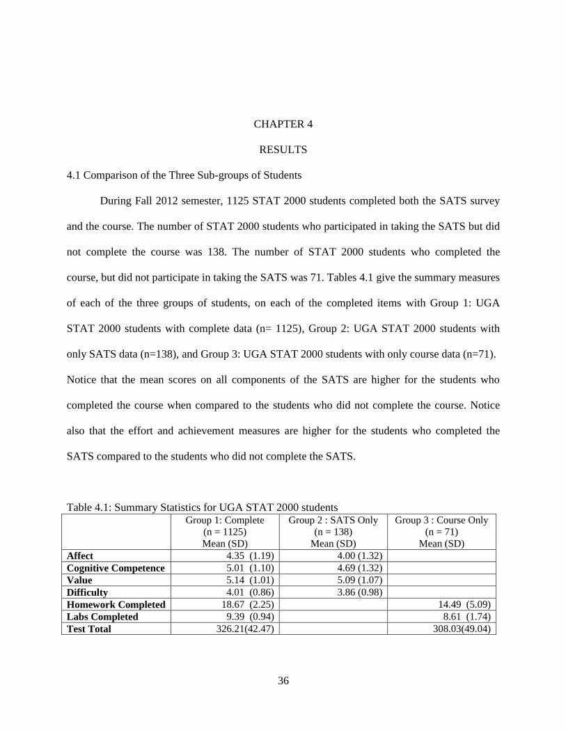
During Fall 2012 semester, 1125 STAT 2000 students completed both the SATS survey

and the course. The number of STAT 2000 students who participated in taking the SATS but did

not complete the course was 138. The number of STAT 2000 students who completed the

course, but did not participate in taking the SATS was 71. Tables 4.1 give the summary measures

of each of the three groups of students, on each of the completed items with Group 1: UGA

STAT 2000 students with complete data (n= 1125), Group 2: UGA STAT 2000 students with

only SATS data (n=138), and Group 3: UGA STAT 2000 students with only course data (n=71).

Notice that the mean scores on all components of the SATS are higher for the students who

completed the course when compared to the students who did not complete the course. Notice

also that the effort and achievement measures are higher for the students who completed the

SATS compared to the students who did not complete the SATS.

Table 4.1: Summary Statistics for UGA STAT 2000 students

Group 1: Complete

(n = 1125)

Mean (SD)

Group 2 : SATS Only

(n = 138)

Mean (SD)

Group 3 : Course Only

(n = 71)

Mean (SD)

Affect 4.35 (1.19) 4.00 (1.32)

Cognitive Competence 5.01 (1.10) 4.69 (1.32)

Value 5.14 (1.01) 5.09 (1.07)

Difficulty 4.01 (0.86) 3.86 (0.98)

Homework Completed 18.67 (2.25) 14.49 (5.09)

Labs Completed 9.39 (0.94) 8.61 (1.74)

Test Total 326.21(42.47) 308.03(49.04)

37

We tested these differences for significance using the Welch Two-Sample t-tests

assuming unequal variance. The research hypothesis was whether the mean on each SATS

component for students who complete STAT 2000 is the same as the mean for students who do

not complete the course. We chose to use α=0.05. For this study, there was a significant

difference between the groups for Affect and Cognitive Competence, when comparing the

students who completed the course to those who did not as we can see from Table 4.2. Also for

this study, there was no significant difference between the groups for Value and Difficulty.

Moreover, all of the differences were positive, showing that the students who complete the

course tend to have more positive attitudes than those who do not complete the course. This will

be discussed further in the next chapter, but for the purposes of the subsequent analyses, of the

SATS data, we have kept these two groups of students separate.

Table 4.2: T-test summaries

Variable Tested Group t –score Degree of

Freedom (df) p-value

Affect by Course 3.023 165.87 0.003**

Cognitive Competence by Course 2.731 161.31 0.007**

Value by Course 0.474 167.89 0.636

Difficulty by Course 1.746 163.93 0.083

Homework Completed by SATS 6.873 71.74 1.919e-09***

Labs Completed by SATS 3.778 72.59 0.0003**

Test Total by SATS 3.053 76.78 0.003**

*significant at =0.05, ** significant at =0.01, ***significant at =0.0001.

Another research hypothesis was whether the mean score for Test Total, Labs Completed,

and Homework Completed for students who complete both SATS and the course is similar to the

mean for students who do not complete SATS. When comparing the students who completed the

course and the SATS to those who completed the course but not the SATS, there was a

significant difference between the two groups on both measures of effort, homework

assignments and labs completed, and on the achievement value of test scores. Again all of the

38

differences are positive, indicating that those students who do not complete the SATS tend to

exhibit less effort and lower achievement than those who do complete the SATS. When

considering the results of the analysis modeling the relationship between the SATS components

and effort and achievement, we must be mindful that we may not be able to generalize the results

to all STAT 2000 students. Rather our conclusions may not be applicable to students at the lower

end of the achievement distribution. .

4.2 Comparison between UGA STAT 2000 and the population

We first looked at the descriptive statistics related to the SATS components. We then

compared the SATS scores of the UGA STAT 2000 students who completed the course to the

nationally reported SATS scores. We also compared the SATS scores of the UGA STAT 2000

students who did not complete the course to the nationally reported SATS scores.

4.2.1 Descriptive statistics of the UGA SATS results

To start our comparison of the UGA STAT 2000 students to the nationally reported

results, we first considered the descriptive statistics related to the SATS components. As we

stated above, a total of 1125 students completed both the SATS and the course. The summary

statistics were given above in Table 4.1. The distribution of SATS is shown below in Figure 4.1.

The distribution of Affect is unimodal and symmetric as shown by Figure 4.1. The affect

component assesses the students’ feelings regarding statistics. With a mean of 4.3, we see that

STAT 2000 students’ feelings toward statistics are slightly positive in the aggregate, with many

students scoring on either side, positive or negative. The distribution of Cognitive Competence is

unimodal and approximately symmetric. The majority of the students seem to have positive

39

attitudes concerning the cognitive competence component, which evaluates students’ attitude

concerning their intellectual knowledge and skills when applied to statistics. With a mean of 5.0,

the aggregate attitude for this component is slightly positive. The distribution of Value is

unimodal and approximately symmetric. Many students seem to believe that statistics can be

useful, relevant, and worthy in their personal and professional life and in fact, the mean score on

this component was the highest of the four components at 5.1. The distribution of Difficulty is

unimodal and nearly perfectly symmetric. Not only is the mean for this component the lowest of

the four at 4.0, but the standard deviation is the lowest as well, at 0.85 indicating, as can be seen

in the histogram, that the students as a group are more likely to have a belief that statistics will be

slightly hard.

40

Histogram of Affect

Affect

Fre

quency

1 2 3 4 5 6 7

050

100

150

Histogram of Cognitive Competence

Cognitive Competence

Fre

quency

1 2 3 4 5 6 7

050

100

150

Histogram of Value

Value

Fre

quency

1 2 3 4 5 6 7

050

100

150

200

Histogram of Difficulty

Difficulty

Fre

quency

1 2 3 4 5 6 7

050

100

200

300

Figure 4.1: Histograms of SATS sub-scores for STAT 2000 students with complete data

4.2.2 Comparison between UGA STAT 2000 and the population

Schau and Emmioglu (2012) reported the national summary statistics for SATS (see

Table 4.3 below). The data were collected from several colleges ranging from small private and

public four-year colleges to large research universities in the United States, so we considered

these data as the baseline and used the summary statistics about this group as representative of a

population. The data included the students who completed both the pre-course and the post-

41

course for her study so we assume that all the students completed the associated statistics course

and compare with the STAT 2000 students who completed the course.

We use the summary statistics for students who completed both the SATS and the course

(Table 4.3). For Affect, Cognitive Competence, and Value, UGA STAT 2000 students have

positive attitudes toward statistics. For Difficulty, the students are neutral. Our Cronbach’s alphas

for each component are high compared to what Schau reports. This was probably caused by the

similarity of the students because our data only includes University of Georgia students, all of

whom were preparing to take the same course, about which they may have heard from other

students. Comparing our data to the population, we can see that for Affect, Cognitive

Competence, Value, and Difficulty, students have more positive attitudes compared to the

population.

Table 4.3: Summary Statistics for SATS Pre for UGA students who complete the course

Sample

Size

Mean Standard

Deviation

Cronbach’s

Alpha

Population

Affect 2209 4.16 1.12 0.81

Cognitive Competence 2192 4.94 1.04 0.84

Value 2186 5.04 0.99 0.87

Difficulty 2204 3.75 0.81 0.76

UGA

Affect 1125 4.35 1.19 0.85

Cognitive Competence 1125 5.01 1.10 0.87

Value 1125 5.14 1.01 0.88

Difficulty 1125 4.01 0.86 0.78

We performed one-sample z-tests to determine if there was a significant difference

between the population scores and UGA STAT 2000 scores for each of the components. Another

research hypothesis was whether UGA STAT 2000 students’ mean score for each component on

the SATS is the same as the corresponding mean score for the population. Our alternative

42

hypothesis was two-sided. That is, that the component’s mean score for UGA STAT 2000

students is not equal to the component’s mean score for the population.

We found the test statistic for each component by using the following formula:

where corresponds to the component’s mean of the STAT 2000 students, μ corresponds to the

population mean for the component, is the population standard deviation for the component,

and n is the sample size for the UGA STAT 2000 students.

Table 4.4: Z-test summaries for students who complete the course

Variable Tested test statistics p-value

Affect 5.71 <0.002**

Cognitive Competence 2.27 0.0232*

Value 3.22 0.0006**

Difficulty 10.78 <0.002**

*significant at =0.05, ** significant at =0.01, ***significant at =0.0001.

We chose to use α=0.05. There was significant difference between the STAT 2000

students and the national population for all four components. Moreover, all differences were

positive, indicating that UGA students who complete STAT 2000 have better attitudes toward

statistics at the beginning of the semester when compared to similar students nationwide.

We wanted to compare the students who did not complete the course (Table 4.5) to the

population since we already concluded the two sub-groups were different and our students who

completed the course have better attitudes than the population. For Cognitive Competence and

Value, UGA students have positive attitudes. For Affect, the students are neutral. For Difficulty,

students believe that it will be hard. Comparing these students to the population, for Affect and

Cognitive Competence, students have less positive attitudes compared to the population; and for

43

Value and Difficulty, students have more positive attitudes compared to the population. Again,

our Cronbach’s alphas for each component are higher than those that Schau reports.

Table 4.5: Summary Statistics for SATS Pre for UGA students who did not complete the course

Sample

Size

Mean Standard

Deviation

Cronbach’s

Alpha

Population

Affect 2209 4.16 1.12 0.81

Cognitive Competence 2192 4.94 1.04 0.84

Value 2186 5.04 0.99 0.87

Difficulty 2204 3.75 0.81 0.76

UGA students

who dropped

Affect 138 4.01 1.34 0.86

Cognitive Competence 138 4.70 1.33 0.89

Value 138 5.10 1.08 0.88

Difficulty 138 3.87 1.00 0.83

We performed one-sample z-tests to determine if there was a significant difference

between the population scores and UGA STAT 2000 scores for each of the components for the

students who do not complete the course. Another research hypothesis was whether the mean

score for each component on the SATS for UGA STAT 2000 students who do not complete the

course is the same as the corresponding mean score for the population. Our alternative

hypothesis was two-sided. That is that the component’s mean score for UGA STAT 2000

students who do not complete the course is not equal to the component’s mean score for the

population.

Table 4.6: Z-test summaries for UGA students who did not complete the course

Variable Tested test statistic p-value

Affect 1.58 0.114

Cognitive Competence 2.73 0.064

Value 0.65 0.516

Difficulty 1.72 0.086

*significant at =0.05, ** significant at =0.01, ***significant at =0.0001.

44

We chose to use α=0.05. For the students who do not complete the course, there was no

evidence that suggested the mean score for UGA STAT 2000 students for Affect, Cognitive

Competence, Value, and Difficulty is different from the mean score of the population. As we

observed earlier, UGA STAT 2000 students who did not complete the course have similar

attitudes toward statistics than the overall population for Affect, Cognitive Competence, Value,

and Difficulty. We would have liked to compare our students who did not complete the course to

the population of students who only took the pre-course, but Schau did not report these values in

her paper.

Overall, UGA STAT 2000 students who complete the course have more positive attitudes

toward statistics than the population for Affect, Cognitive Competence, Value, and Difficulty

when measured at the beginning of the semester. UGA STAT 2000 students who do not

complete the course have similar attitudes toward statistics at the beginning of the semester when

compared the overall population of introductory statistics students.

4.3 Modeling the Relationships between Attitude, Effort, and Achievement

Our main research goal is to see whether the students’ pre-course SATS-28 scores and

the students’ effort are associated with the students’ achievement. We first looked at the

correlations between certain variables to make sure that none of the correlations are extremely

high, causing multicollinearity (Kutner, Nachtsheim, Neter, and Li, 2005). Next we fit the model

to predict test total using SATS components scores, the number of homework and Labs

Completed, and several demographic factors. We used a General Linear model to start since

some of the factors, such as gender and year in school, are categorical.

45

4.3.1 Descriptive statistics of the UGA Course results

Before we fit a model to our data, we first consider the descriptive statistics related to the

Test Total, Labs Completed, and Homework Completed. As we stated above, a total of 1125

students completed both the SATS and the course. The summary statistics were given above in

Table 4.1.The distribution of Test Total is unimodal and skewed to the left as shown by Figure

4.2. While most of the STAT 2000 students did fairly well on the tests with a mean of 326.21

points, several students did not, which accounts for the large standard deviation of 42.47 points.

Histogram of Total Test Points

Total Test Points

Fre

quency

200 250 300 350 400

050

100

150

200

250

Figure 4.2: Histogram of Test Total on UGA STAT 2000 students with complete data

Both the distribution of the Labs Completed and the distribution of the Homework

Completed are unimodal and severely skewed to the left as shown by Figure 4.3. It seems that

most of the students attend the majority of the lab sessions even though their lab grade only

counted 800 out of 1000 points with a mean of 9.3911 sessions attended and standard deviation

of 0.9356. This could be accounted for by several explanations: students received a lower grade

than they wanted on one lab and wanted to earn a 100 on the lab grade, students wanted to learn

46

the material, or students forgot the grade scale. Most of students submitted the majority of the

homework assignments with mean of 18.67 assignments submitted and standard deviation of

2.25.

Labs Completed

Labs Completed

Fre

quency

2 4 6 8 10

0100

200

300

400

500

600

Homework Completed

Homework Completed

Fre

quency

5 10 15 20

0100

200

300

400

500

600

Figure 4.3: Histograms of Homework Completed and Labs Completed on UGA STAT 2000

students with complete data

4.3.2 Correlation Between Variables

We wanted to see if there was a strong linear relationship between any two of our

variables. We examined the pairwise correlations between the variables to make sure that none

of the correlations were extremely high, causing multicollinearity (Kutner, Nachtsheim, Neter,

and Li, 2005). Figure 4.4 and Table 4.7 below show that Affect and Cognitive Competence are

very strongly linear and correlated. The correlations and linear relationships for Affect and

Difficulty, as well as Cognitive Competence and Difficulty, are strong. Affect and Value, in

addition to Cognitive Competence and Value, are moderately correlated and have a moderate

linear relationship. Value and Difficulty are weakly correlated and a weak linear relationship.

47

1 3 5 7

12

34

56

7

Affect

Cognitiv

e C

om

pete

nce

1 3 5 71

23

45

67

Affect

Valu

e

1 3 5 7

12

34

56

7

Affect

Difficulty

1 3 5 7

12

34

56

7

Cognitive Competence

Valu

e

1 3 5 7

12

34

56

7

Cognitive Competence

Difficulty

1 3 5 7

12

34

56

7

Value

Difficulty

Figure 4.4: Scatterplots of SATS sub-scores for STAT 2000 students with complete data

Table 4.7: Correlations for UGA STAT 2000 students with complete data

Affect Cognitive

Competence

Value Difficulty Test

Total

Course

GPA

Lab

Completed

Homework

Completed

Affect 1.000 0.827 0.444 0.642 0.281 0.255 0.006 -0.036

Cognitive

Competence 0.827 1.000 0.426 0.654 0.281 0.251 -0.018 -0.042

Value 0.444 0.426 1.000 0.212 0.182 0.160 0.026 -0.026

Difficulty 0.642 0.654 0.212 1.000 0.228 0.209 -0.026 -0.036

Test Total 0.281 0.281 0.182 0.228 1.000 0.963 0.196 0.281

Course

GPA 0.255 0.251 0.160 0.209 0.963 1.000 0.270 0.434

Labs

Completed 0.006 -0.018 0.026 -0.026 0.196 0.270 1.000 0.430

Homework

Completed -0.036 -0.042 -0.026 -0.036 0.281 0.434 0.430 1.000

48

Similarly, Table 7 shows that Course GPA and Test Total are extremely strongly positive

correlated. Course GPA and Homework Completed plus Labs Completed and Homework

Completed are moderately correlated. The students’ Test Total tends to increase as Course GPA

increased as shown in Figure 4. In addition the variability in Test Total tends to decrease as

Course GPA increases, but there are some high outliers, students who earned unusually high Test

Total when compared to other students with the same Course GPA. From the middle boxplot

graph in Figure 4.5, we see that the number of Homework Completed by the students tends to

increase as Course GPA increases. There are some low outliers for students who have unusually

low Homework Completed when compared to other students with the same Course GPA, but the

variability in Homework Completed generally tends to decrease as Course GPA increases. Also

for the most part, the number of HW Completed increases as the number of Labs Completed

increases. While the variability in Homework Completed tends to decrease as Labs Completed

increases, there are several low outliers: students who have unusually low number of Homework

Completed when compared to other students with the same number of Labs Completed. Note

that only 12 students completed 9 or fewer homework assignments and only 6 students

completed 5 or fewer labs without much overlap between these groups. These students will be

discussed again in section 4.3.4.

49

0 1 1.7 2 2.3 2.7 3 3.3 3.7 4

200

250

300

350

400

Course GPA

TestT

ota

l

0 1 1.7 2 2.3 2.7 3 3.3 3.7 4

510

15

20

Course GPA

HW

Com

ple

ted

1 2 3 4 5 6 7 8 9 10

510

15

20

Labs Completed

HW

Com

ple

ted

Figure 4.5: Boxplots of STAT 2000 course data with moderate to high correlations for students

with complete data

Since Course GPA and Test Total are extremely strongly positive correlated (r = 0.963),

we should not use them together in General Linear model. The other variables seem to be safe to

use in the model.

4.3.3 Fitting an General Linear Model

Our research goal was to see whether the students’ pre-course SATS-28 scores are

associated with student achievement. Since we included quantitative and categorical variables

into the model, we used a General Linear model to predict Test Total as our achievement. We

used several quantitative variables: Affect, Cognitive Competence, Value, Difficulty, Labs

Completed, Homework Completed, Previous mathematics and/or statistics classes in High

School, and Previous mathematics and/or statistics classes in College as explanatory variables. In

addition, we considered the categorical variables: Gender, Age, Required, and Year of college as

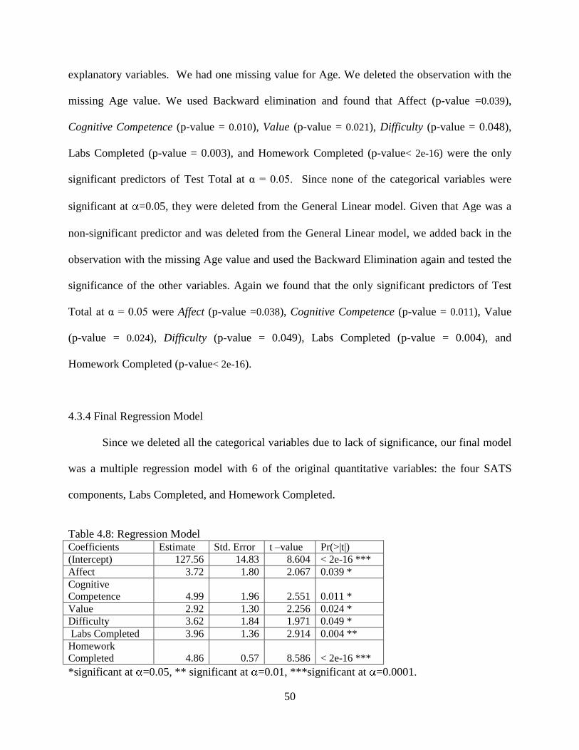
50

explanatory variables. We had one missing value for Age. We deleted the observation with the

missing Age value. We used Backward elimination and found that Affect (p-value =0.039),

Cognitive Competence (p-value = 0.010), Value (p-value = 0.021), Difficulty (p-value = 0.048),

Labs Completed (p-value = 0.003), and Homework Completed (p-value< 2e-16) were the only

significant predictors of Test Total at α = 0.05. Since none of the categorical variables were

significant at =0.05, they were deleted from the General Linear model. Given that Age was a

non-significant predictor and was deleted from the General Linear model, we added back in the

observation with the missing Age value and used the Backward Elimination again and tested the

significance of the other variables. Again we found that the only significant predictors of Test

Total at α = 0.05 were Affect (p-value =0.038), Cognitive Competence (p-value = 0.011), Value

(p-value = 0.024), Difficulty (p-value = 0.049), Labs Completed (p-value = 0.004), and

Homework Completed (p-value< 2e-16).

4.3.4 Final Regression Model

Since we deleted all the categorical variables due to lack of significance, our final model

was a multiple regression model with 6 of the original quantitative variables: the four SATS

components, Labs Completed, and Homework Completed.

Table 4.8: Regression Model Coefficients Estimate Std. Error t –value Pr(>|t|)

(Intercept) 127.56 14.83 8.604 < 2e-16 ***

Affect 3.72 1.80 2.067 0.039 *

Cognitive

Competence 4.99 1.96 2.551 0.011 *

Value 2.92 1.30 2.256 0.024 *

Difficulty 3.62 1.84 1.971 0.049 *

Labs Completed 3.96 1.36 2.914 0.004 **

Homework

Completed 4.86 0.57 8.586 < 2e-16 ***

*significant at =0.05, ** significant at =0.01, ***significant at =0.0001.

51

The model is Test Total = 127.56 + 3.72 Affect + 4.99 Cognitive Competence + 2.92

Value + 3.62 Difficulty + 3.96 Labs Completed + 4.86 Homework Completed. We looked at the

residual plot (Figure 4.6) to be sure the multiple regression model is appropriate for the data and

to examine whether the errors terms have constant variance. The residual plot shows the model

may not be appropriate for students at the lower end of the achievement distribution. The model

overestimated the students with lower test total by assuming the high number of homework

completed and labs completed indicated high test total. Similarly the model underestimated some

students with high test total by assuming the lower number of homework completed and labs

completed indicated lower test total. This lack of fit may also be related to the small number of

students who completed fewer than 9 homework assignments or fewer than 5 labs.

240 260 280 300 320 340 360

-150

-100

-50

050

100

The Residual Plot

Predicted Score

Resid

uals

Figure 4.6: The Residual Plot of the model.

The model has a root mean square error (RMSE) of 38.46, which, for a particular

observation, estimates the typical size of the errors between the actual Test Total and the

52

predicted Test Total (Reeves, personal communication). This error is so large when compared to

the range of possible scores that it is clear that the model has little predictive power. The model’s

R-squared is 0.1846, which means that only 18.46% of the variation is explained by the factors

in the model. Since the R-squared is so low, we seem to be missing some factors that account for

the total test scores other than the components of SATS, the number of homework and labs

completed. The factors could possibly be the students’ study habits and their post-course scores.

While the model does not explain much of the variability in total test scores, it is interesting to

note that the factors that are most strongly predictive of test scores are the measures of effort,

followed by the attitudes toward cognitive competence, value of statistics, affect, and the

difficulty of statistics.

4.4 Summer 2013 Data

There were 135 students who completed the course during the summer and 31 of those

students took the survey at the beginning of the course. We had one additional survey with not

answered cells as responses and we assume the student dropped the course and eLC erased her

responses. In any case, this student could not be included in the analysis. Since the survey was

anonymous, we cannot connect the students’ Test Total to their responses to the survey. Since

we do know which students took the survey, we tested the difference of the Test Total between

the students who took the survey and the students who did not take the survey for significance.

Our research hypothesis was whether the Test Total mean of students who complete the survey is

the same as the Test Total mean of students who do not complete the survey. We used the

Welch Two-Sample t-test on Test Total. The mean for the students who completed the survey is

332.53. The mean for the students who did not complete the survey is 329.35. The t-statistic is

53

0.2817 with degrees of freedom of 41.25. The p-value is 0.780, so we consider the students who

completed the survey as representative of the population of summer students.

Of the thirty-one students who answered the survey, 21 students indicated that their

attitudes were mostly positive and 9 students chose that their attitudes were mostly negative. One

student decided to mark both mostly positive and mostly negative. The overall themes to the

mostly positive responses were that statistics was practical in the real world (n = 9, 29.0%), that

the student liked the course (n = 5, 16.1%), statistics was important to majors (n = 4, 12.9%), to

future career (n = 4, 12.9%), and that the student enjoys math (n = 4, 12.9%). The overall themes

to the mostly negative responses were that the student was retaking the course (n = 4, 12.9%),

found it frustrating or challenging (n = 4, 12.9%), was not good at math (n = 3, 9.7%), did not

like math (n = 1, 3.2%), was not good at statistics (n = 1, 3.2%), had bad experiences in high

school (n = 1, 3.2%), or had to pass this time to graduate (n = 1, 3.2%). Three students were

indifferent toward statistics (n = 3, 9.7%). Students could be included into multiple themes for

both positive and negative. For this reason, the percent is out of 31 students and the sum of the

percents is over 100.

Table 4.9: Themes to Students’ Attitudes

Themes Number of

Students

Percent of

Students

Mostly

Positive

Statistics was practical in the real world 9 29.0

Student liked the course 5 16.1

Statistics was important to majors 4 12.9

Statistics was important to future career 4 12.9

Student enjoys math 4 12.9

Mostly

Negative

The student was retaking the course 4 12.9

Student found statistics frustrating or challenging. 4 12.9

Student was not good at math. 3 9.7

Student did not like math 1 3.2

Student was not good at statistics. 1 3.2

Student had bad experiences in high school. 1 3.2

Student had to pass this time to graduate. 1 3.2

Neutral Student was indifferent toward statistics. 3 9.7

54

The most common theme to mostly positive attitudes was the students believe that

statistics is practical to know in the real world. Two of the most common themes to mostly

negative attitudes was the students were retaking the course and the students found statistics

frustrating or challenging.

When the students were asked whether the knowledge of statistics will be useful in their

future career, 23 students answered yes, 6 students answered no, and 2 students answered yes

and no. The students who answered yes and no were either unsure or needed it for a prerequisite.

Table 4.10: Two-Way Table for Attitude and Perceived Usefulness. Perceived Usefulness

Yes No Yes/No Total

Attitude

Mostly Positive 17 3 1 21

Mostly Negative 5 3 1 9

Mostly Positive/Mostly Negative 1 0 0 1

Total 23 6 2 31

Most of the students believe that statistics will be useful sometime in the future, whether

their attitude was mostly positive or mostly negative. Students who perceived statistics as useful

were more likely to have a mostly positive attitude toward statistics. The students, who chose no

or yes/no, were equally spread along the mostly positive and mostly negative attitudes. There

seems to be a relationship between perception of usefulness and positive attitudes toward

statistics. No inferential procedure was done to test the significance of the relationship as the

sample size was too small for any meaningful procedure to be run. Nevertheless, we think this

information will provide some direction for improving the attitudes of the STAT 2000 students,

which will be discussed in the next chapter.

55

CHAPTER 5

CONCLUSION

The students who completed the course had better attitudes than those who did not finish

the course. There was a significant difference between the students who completed the course

and those who did not for the Affect and Cognitive Competence components, which measures the

students’ feelings regarding statistics and their attitude concerning their intellectual knowledge

and skills applied to statistics, respectively. There was not a significant difference between the

students who completed the course and those who did not complete the course for Value and

Difficulty , which measures the students’ belief that statistics can be useful, relevant, and worthy

in their personal and professional life, and the students’ attitudes about the difficulty of statistics,

respectively. I would recommend that attitudes, especially for Affect and Cognitive Competence

should be addressed at the beginning of the semester in order to attempt to reduce the student

drop rate in the class for students with low attitudes. Our students who completed the course had

better attitudes than reported nationally. Our students who did not complete the course had

similar attitudes than reported nationally. The effort (homework completed and Labs Completed)

and achievement (test total) measurements are higher for the students who completed the SATS

when compared to the students who did not complete the SATS.

There was a relationship between attitudes, effort, and achievement. It is interesting to

note in our model that the factors that are most strongly predictive of test scores are the measures

of effort, followed by each of the SATS components. Our model may not be appropriate to

students at the lower end of the achievement distribution. Some of the negative attitudes may be

56

due to students’ dislike toward math and frustration that statistics is causing them. Some of the

positive attitudes may be due to the students’ enjoyment of the class or math, statistics’

importance to the real world, as well to the students’ major and future career. The majority of the

students stated that they believe statistics will be useful to them in the future.

Attitudes toward statistics influence the students’ beliefs, behavior, motivation, and their

learning skills. Their attitudes also influence how the students will apply their knowledge of

statistics in their personal and professional lives. We know that the negative attitudes (from

summer data) can be a result of a bad prior experience, so we can use these findings to make

suggestions on improving students’ attitudes in the classroom. These suggestions are made with

the caveat that since I have not been a STAT 2000 student at UGA or a STAT 2000 TA, some of

these suggestions may already be in place.

1. Give a question each week from a context with which the students can relate in order to

get students interested in statistics (Wroughton and Kerby, 2013). This would hopefully

increase the students’ interest in statistics by showing them how statistics can be applied

to their lives. Show real life examples using statistics. Explain the students how they

might use statistics in their careers.

2. Try to reassure the students that introductory statistics is not a math class. Since high

school algebra is a prerequisite to the class, tell the students what math skills are needed

to understand the material (Schau, 2003b). Since two themes for students’ mostly

negative attitudes were that the student did not like math or was not good at math,

knowing what to expect in terms of math calculations might be reassuring the students

with a fear of math.

57

3. Be positive, sympathetic, and encouraging to your students, both inside and outside the

classroom (Schau, 2003b). If the teacher or TA acts as though s/he does not enjoy

statistics or teaching or care about the students, the students will pick up on these

attitudes and probably imitate them.

4. Measure the students’ attitudes at the beginning and end of the course to see if the

students’ attitudes have changed (Schau, 2003b). Use one of the statistics attitude surveys

that I mentioned in the literature review (SAS, ATS, SATS-28, and SATS-36) to measure

the students’ attitudes. Since our students already have positive attitudes, do not to be too

upset if there was not any change. First, little change is reported in the literature about the

use of both pre- and post-SATS, particularly after the first week of class. Second, UGA

students’ attitudes toward statistics are reasonable, so you are already doing a good job.

5. Explain that everyone makes mistakes, but trying is more important than being correct.

Admit when you make mistakes in class and use those mistakes to teach the students

(Schau, 2003b). If you make a mistake, probably most of your students will make the

same mistake on their homework or test. By admitting your mistakes, the students will

learn from your mistake instead of theirs on an important test. Also explain to the

students that they would prefer to make these mistakes on the homework instead of the

exams, which brings me to my next points.

6. Have students attempt the homework by themselves without help the first time. From

personal experience, everything looks easier when some else does it first. Since the

students have three attempts, they can attempt all the problems by themselves on the first

attempt. For the second and third attempt, they can go to Open Lab and have a

TA explains the concepts they do not understand.

58

7. Allow students to create their own “cheat sheet” on exams. Creating these cheat sheets

will help the students study and learn, and having the cheat sheet will calm the students

(Schau, 2003b). It will be easier for the students to understand and find formulas if they

are allowed to write them out. Students also have to study to find the important facts to

include on the cheat sheet.

8. While you cannot give attitude surveys to the students after each topic is introduced, you

could give a survey at the end of the class asking the students what topics they liked or

disliked. Another option could be to examine the homework to see what section of

homework the students are more likely to skip. If most of the students have similar topics

that they like or dislike or find difficult, if possible, the teacher might want to spend more

time on that topic next semester. For the current semester, have a review session to

clarify the students’ questions on the topic.

9. For the tests, there should be some questions that are not multiple choice and the students

could possibly received some partial credit.

There were some limitations of this study. We did not give a SATS post-course to

students so we could not see whether there was a change in the student’s attitudes toward

statistics. The R-squared of the model was low, which indicates that we seem to be missing

some factors that account for the total test scores other than the components of SATS, the

number of homework and labs completed. Since the pre-course was given before any of the tests,

the post-course might do a better job of predicting the total test scores. The factors could

possibly be the students’ study habits and their post-course scores. By student’s study habits, we

mean the amount of time the student devoted to learning statistics outside of class and labs,

whether the student tries to do his/her homework without help the first time, and how many

59

times before the student attended the open labs. These study habits obviously should have a big

role in the student’s grades. Another limitation to our study was that 71 students who did not

participate in the SATS survey. I would have liked to know why they chose not to participate

(for example was the survey too long). We only have course data on students who completed the

course. For the students who dropped the course, I would have liked to see whether their attitude

was related to the first or second test scores.

60

REFERENCES

Affective. (n.d.). Merriam-Webster.com. Retrieved September 5, 2013, from

http://www.merriam-webster.com/dictionary/affective

Beamer, J., (2013). Examining Introductory Students’ Attitudes in a Randomization-Based

Curriculum (Unpublished Senior Project). California Polytechnic State University, San

Luis Obispo.

Cashin, S. E., & Elmore, P. B. (2005). The Survey of Attitudes Toward Statistics scale: A

construct validity study. Educational and Psychological Measurement, 65(3), 509–524.

Crocker, L. M. and Algina, J. (1986). Introduction to classical and modern test theory. Holt,

Rinehart, and Winston, New York.

Emmioğlu, E. & Capa-Aydin, Y. (2012). Attitudes and achievement in Statistics: A meta-

analysis study. Statistics Education Research Journal, 11(2), 95-102 [Online:

http://www.stat.auckland.ac.nz/~iase/serj/SERJ11(2)_Emmioglu.pdf]

Dweck, C. (2002). Messages that Motivate: How Praise Molds Students’ Beliefs, Motivation,

and Performance (in Surprising Ways). In J. Aronson (Eds.), Improving Academic

Achievement: Impact of Psychological Factors on Education (pp. 37–60). Elsevier

Science (USA).

Gal, I., & Ginsburg, L. (1994). The role of beliefs and attitudes in learning statistics: Towards an

assessment framework. Journal of Statistics Education, 2(2), 1–15.

[Online: http://www.amstat.org/publications/jse/v2n2/gal.html ]

61

Gal, I., Ginsburg, L., & Schau, C. (1997). Monitoring Attitudes and Beliefs in Statistics

Education. In I. Gal & J. B. Garfield (Eds.), The Assessment Challenge in Statistical

Education (pp. 37–51). IOS Press.

Griffith, J.D., Adams, L.T., Gu, L.L., Hart, C.L., & Nichols-Whitehead, P (2012). Students’

Attitudes Towards Statistics Across the Disciplines: A Mixed-Methods Approach.

Statistics Education Reseach Journal, 11(2), 45-56. [Online:

http://www.stat.auckland.ac.nz/serj]

Jansen, Greg (2013). Improving Validity and Reliability in STAT 2000 Assessments

(Unpublished Master’s Thesis). University of Georgia, Athens, GA. [Online:

https://getd.libs.uga.edu/pdfs/jansen_gregory_g_201305_ms.pdf ]

Kutner, M., Nachtsheim, C., Neter, J., & Li, W. (2005). Applied Linear Statistical Models (5th

Edition). New York: McGraw-Hill Irwin

Messick, S. (1995). Validity of psychological assessment: Validation of inferences from persons’

responses and performances as scientific inquiry into score meaning. American

Psychologist, 50(9), 741–749.

Nolan, M.M., Beran, T., & Hecker, K.G. (2012). Surveys assessing students’ attitudes towards

statistics: A systematic review of validity and reliability. Statistics Education Research

Journal, 11(2), 103-123 [Online:

http://www.stat.auckland.ac.nz/~iase/serj/SERJ11(2)_Nolan.pdf]

Pearl, D.K., Garfield, J.B., delMas, R., Groth, R.E., Kaplan, J.J., McGowan, H., and Lee,

H.S. (2012). Connecting Research to Practice in a Culture of Assessment for Introductory

College-level Statistics.

[Online: http:// www.causeweb.org/research/guidelines/ResearchReport_Dec_2012.pdf]

62

Ramirez, C., Schau, C, & Emmioğlu, E.. (2012). The importance of attitudes in Statistics

Education. Statistics Education Research Journal, 11(2), 57-71 [Online:

http://www.stat.auckland.ac.nz/~iase/serj/SERJ11(2)_Ramirez.pdf]

Roberts, D.M., & Bilderback, E.W. (1980). Reliability and validity of a statistics attitude survey.

Educational and Psychological Measurement, 40, 235-238.

Ryan, R.M., & Deci, E.L. (2000). Intrinsic and Extrinsic Motivations: Classic Definitions and

New Directions. Contemporary Educational Psychology, 25, 54-67.

Schau, C., Stevens, J., Dauphinee, T., & Del Vecchio, A. (1995). The development and

validation of the Survey of Attitudes Toward Statistics. Educational & Psychological

Measurement, 55 (5),868-876.

Schau, C. and Emmioglu, E. (2012). Do Introductory Statistics Courses in the United

States Improve Students’ Attitudes? Statistics Education Research Journal, 11(2), 86-94.

[Online: http://www.stat.auckland.ac.nz/serj]

Schau, C. (1992). Survey of Attitudes Toward Statistics (SATS-28).

[Online: http://evaluationandstatistics.com]

Schau, C. (2003a). Survey of Attitudes Toward Statistics (SATS-36).

[Online:http://evaluationandstatistics.com]

Schau, C. (2003b). Students' attitudes: The "other" important outcome in statistics education.

Joint Statistical Meetings, San Francisco, CA. Online:

http://evaluationandstatistics.com/JSM2003.pdf.

Schau, C. (2008). Common issues in SATS© research. Joint Statistical Meetings, Denver, CO.

Online: http://evaluationandstatistics.com/JSM2008.pdf.

63

University of Georgia (2013). Bulletin - Courses Home. Retrieved Sept 8, 2013.

http://bulletin.uga.edu/CoursesHome.aspx.

Vanhoof, S., Sotos, A. E. C., Onghena, P., Verschaffel, L., Van Dooren, W., & Van den

Noortgate,W. (2006). Attitudes toward statistics and their relationship with short- and

long-term exam results. Journal of Statistics Education, 14(3). [Online:

http://www.amstat.org/publications/jse/v14n3/vanhoof.html]

Wise, S. L. (1985). The development and validation of a scale measuring attitudes toward

statistics. Educational and Psychological Measurement, 45(2), 401–405.

Wroughton, J. & Kerby, A., (2013) Does Making Connections Improve Student Attitudes?

Contribution Presentation at the Joint Statistical Meetings of the American Statistical

Association: Montreal, CA.

64

APPENDIX A

R-Code

A.1 To compare the sub-groups using T-tests for Fall 2012 and Summer 2013 Data

a <- read.csv(file="EditedMasterCopy3.csv",header=TRUE)

t.test(a$HWAttempt ~a$SATS)

t.test(a$LabAttempt ~a$SATS)

t.test(a$TestTotal~a$SATS)

t.test(a$Affect~a$Enrollment)

t.test(a$CC~a$Enrollment)

t.test(a$Value~a$Enrollment)

t.test(a$Difficulty~a$Enrollment)

b <- read.csv(file="SU13CourseGrades.csv",header=TRUE)

t.test(b$TotalTest ~b$Attitudes.Toward.Statistics)

A.2 To create the histograms, scatterplots, and boxplots for students with complete data

c <- read.csv(file="SATSCourse.csv",header=TRUE)

# histograms for SATS components, Test Total, Labs Completed, and Homework Completed

hist(c$Affect,xlab="Affect",main="Histogram of Affect")

hist(c$CC,xlab="Cognitive Competence",main="Histogram of Cognitive Competence")

hist(c$Value,xlab="Value",main="Histogram of Value")

hist(c$Difficulty,xlab="Difficulty",main="Histogram of Difficulty")

hist(c$TestTotal,xlab=" Total Test Points",main="Histogram of Total Test Points")

65

hist(c$HWCompleted,xlab="Homework Completed",main="Homework Completed")

hist(c$LabCompleted,xlab="Labs Completed",main="Labs Completed")

round (cor(cbind(c$Affect, c$CC, c$Value, c$Difficulty, c$TestTotal, c$GPA, c$LabCompleted,

c$HWCompleted)),3)

# scatterplots for continuous variables

par(mfrow=c(3,2))

plot(c$Affect, c$CC,xlab="Affect",ylab="Cognitive Competence")

plot(c$Affect, c$Value,xlab="Affect",ylab="Value")

plot(c$Affect, c$Difficulty,xlab="Affect",ylab="Difficulty ")

plot(c$CC, c$Value,xlab=" Cognitive Competence ",ylab="Value")

plot(c$CC, c$Difficulty,xlab=" Cognitive Competence ",ylab="Difficulty")

plot(c$Value, c$Difficulty,xlab=" Value ",ylab="Difficulty")

#boxplots for ordinal data

par(mfrow=c(1,3))

boxplot(c$TestTotal ~c$GPA,xlab="Course GPA ",ylab=" TestTotal ")

boxplot(c$HWCompleted ~c$GPA, xlab="Course GPA ",ylab=" HW Completed ")

boxplot(c$HWCompleted~ c$LabCompleted,xlab=" Labs Completed ",ylab=" HW Completed ")

A.3 Model Selection without the observation with missing Age observation

d <- read.csv(file="SATSCourseAge.csv",header=TRUE)

test<-lm(d$TestTotal~d$Affect + d$CC+ d$Value+d$Difficulty+ factor( d$Gender)

+factor(d$CollegeYear) +factor(d$Required) +factor(d$Age)+ d$HS +d$College +

d$LabCompleted +d$HWCompleted)

66

summary(test)

#delete Gender with p-value of 0.862.

test1<-lm(d$TestTotal~d$Affect + d$CC+ d$Value+d$Difficulty+ factor(d$CollegeYear)

+factor(d$Required) +factor(d$Age)+ d$HS +d$College + d$LabCompleted +d$HWCompleted)

summary(test1)

#delete Age with p-values of 0.706, 0.460, 0.298, & 0.872

test2<-lm(d$TestTotal~d$Affect + d$CC+ d$Value+d$Difficulty+ factor(d$CollegeYear)

+factor(d$Required) + d$HS +d$College + d$LabCompleted +d$HWCompleted)

summary(test2)

# delete College with p-values of 0.689

test3<-lm(d$TestTotal~d$Affect + d$CC+ d$Value+d$Difficulty+ factor(d$CollegeYear)

+factor(d$Required) + d$HS + d$LabCompleted +d$HWCompleted)

summary(test3)

#delete Required with p-value of 0.596

test4<-lm(d$TestTotal~d$Affect + d$CC+ d$Value+d$Difficulty+ factor(d$CollegeYear) +

d$HS + d$LabCompleted +d$HWCompleted)

summary(test4)

#delete HS with p-values of 0.080

test5<-lm(d$TestTotal~d$Affect + d$CC+ d$Value+d$Difficulty+ factor(d$CollegeYear) +

d$LabCompleted +d$HWCompleted)

summary(test5)

#delete CollegeYear with p-values of 0.864, 0.424, 0.079, & 0.483

67

test6<-lm(d$TestTotal~d$Affect + d$CC+ d$Value+ d$Difficulty+ d$LabCompleted

+d$HWCompleted)

summary(test6)

A.4 Model Selection with all observations with complete data

#Since Age was not a significant predictor variable, we went back to the dataset with all the

observations.

e <- read.csv(file="SATSCourse.csv",header=TRUE)

test<-lm(e$TestTotal~e$Affect + e$CC+ e$Value+e$Difficulty+ factor( e$Gender)

+factor(e$CollegeYear) +factor(e$Required) + e$HS + e$College + e$LabCompleted

+e$HWCompleted)

summary(test)

#delete Gender with p-value of 0.843.

test1<-lm(e$TestTotal~e$Affect + e$CC+ e$Value+e$Difficulty+ factor(e$CollegeYear)

+factor(e$Required) + e$HS + e$College + e$LabCompleted +e$HWCompleted)

summary(test1)

# delete College with p-value of 0.693

test2<-lm(e$TestTotal~e$Affect + e$CC+ e$Value+e$Difficulty+ factor(e$CollegeYear)

+factor(e$Required) + e$HS + e$LabCompleted +e$HWCompleted)

summary(test2)

#delete Required with p-value of 0.663

test3<-lm(e$TestTotal~e$Affect + e$CC+ e$Value+e$Difficulty+ factor(e$CollegeYear) +e$HS

+ e$LabCompleted +e$HWCompleted)

68

summary(test3)

#delete HS with p-value of 0.07505

test4<-lm(e$TestTotal~e$Affect + e$CC+ e$Value +e$Difficulty +factor(e$CollegeYear) + e$

LabCompleted +e$HWCompleted)

summary(test4)

#delete College Year with p-values of 0.863, 0.423, 0.061, & 0.484

test5<-lm(e$TestTotal~e$Affect + e$CC+ e$Value +e$Difficulty + e$LabCompleted

+e$HWCompleted)

summary(test5)

result=cbind(e$UserID,e$TestTotal,e$Affect,e$CC,e$Value,e$Difficulty,e$LabCompleted,e$H

WCompleted,test5$fit,test5$res)

round(result,3)

#residual plot

plot(test5$fit,test5$res,xlab="Predicted Score", ylab="Residuals", main="The Residual Plot")

abline(h=0,col="red")

A.5 Cronbach’s Alpha

# Cronbach’s Alpha for student who completed the course

install.packages("CTT")

library(CTT)

sc<- read.csv(file="SATSC.csv",header=TRUE)

Affect<-cbind(sc$X1,sc$X2,sc$X11,sc$X14,sc$X15,sc$X21)

CC<-cbind(sc$X3,sc$X9,sc$X20, sc$X23,sc$X24,sc$X27)

69

Value<-cbind(sc$X5,sc$X7,sc$X8, sc$X10,sc$X12,sc$X13, sc$X16,sc$X19,sc$X25)

Difficulty<-cbind(sc$X4,sc$X6,sc$X17, sc$X18,sc$X22,sc$X26, sc$X28)

#reliability coefficient

options(digits=5)

reliability(Affect, itemal=TRUE)

reliability(CC, itemal=TRUE)

reliability(Value, itemal=TRUE)

reliability(Difficulty, itemal=TRUE)

# Cronbach’s Alpha for student who did not complete the course

snc <- read.csv(file="SATSNC.csv",header=TRUE)

Affect<-cbind(snc$X1,snc$X2,snc$X11,snc$X14,snc$X15,snc$X21)

CC<-cbind(snc$X3,snc$X9,snc$X20, snc$X23,snc$X24,snc$X27)

Value<-cbind(snc$X5,snc$X7,snc$X8, snc$X10,snc$X12,snc$X13,

snc$X16,snc$X19,snc$X25)

Difficulty<-cbind(snc$X4,snc$X6,snc$X17, snc$X18,snc$X22,snc$X26, snc$X28)

reliability(Affect, itemal=TRUE)

reliability(CC, itemal=TRUE)

reliability(Value, itemal=TRUE)

reliability(Difficulty, itemal=TRUE)