undergraduate education and the gender wage gap: an ... · pdf fileduke university durham, ......

Undergraduate Education and the Gender Wage Gap: An Analysis of the Effects of College Experience and

Gender on Income

Kelsey Siman*

Professor Kent Kimbrough, Thesis Instructor

Professor Arnaud Maurel, Thesis Advisor

Duke University Durham, North Carolina

2014

*Kelsey Siman graduated in May 2014 with High Distinction in Economics and minors in Mathematics and Spanish. Following graduation, Kelsey will be working as an Investment Banking Analyst at Jefferies, LLC in New York, NY. Kelsey can be reached at [email protected].

Siman

2

Acknowledgements

I would like to thank my advisor, Professor Arnaud Maurel, for his invaluable advice and assistance in writing this thesis. I would also like to thank Professor Kent Kimbrough for

his support and constructive revisions. Finally, I would like to thank my fellow classmates in Economics 495S and 496S for their insightful comments and enthusiasm.

All of these people made writing this thesis a wonderful experience.

Siman

3

Abstract

Labor and education economists have long been interested in the link between undergraduate education and earnings. In addition, studies have addressed the

connections between gender and college major and GPA, as well as between gender and income. This paper brings all of these together in order to show that college major choice

does have a significant effect on earnings, and that this effect differs with gender and across majors. The results show that controlling for college major, ability measures,

graduation year, and GPA can help to explain a majority of the gender pay gap. Finally, the thesis then utilizes the Oaxaca-Blinder Decomposition to break down the price and

composition effect of undergraduate education on the gender pay gap.

JEL Classification: A22, J16 Keywords: College, Gender, Income

Siman

4

I. Introduction

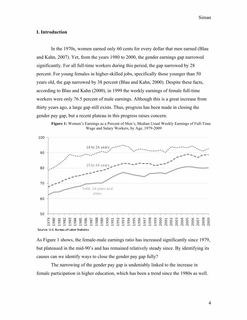
In the 1970s, women earned only 60 cents for every dollar that men earned (Blau

and Kahn, 2007). Yet, from the years 1980 to 2000, the gender earnings gap narrowed

significantly. For all full-time workers during this period, the gap narrowed by 28

percent. For young females in higher-skilled jobs, specifically those younger than 50

years old, the gap narrowed by 38 percent (Blau and Kahn, 2000). Despite these facts,

according to Blau and Kahn (2000), in 1999 the weekly earnings of female full-time

workers were only 76.5 percent of male earnings. Although this is a great increase from

thirty years ago, a large gap still exists. Thus, progress has been made in closing the

gender pay gap, but a recent plateau in this progress raises concern. Figure 1: Women’s Earnings as a Percent of Men’s, Median Usual Weekly Earnings of Full-Time

Wage and Salary Workers, by Age, 1979-2009

As Figure 1 shows, the female-male earnings ratio has increased significantly since 1979,

but plateaued in the mid-90’s and has remained relatively steady since. By identifying its

causes can we identify ways to close the gender pay gap fully?

The narrowing of the gender pay gap is undeniably linked to the increase in

female participation in higher education, which has been a trend since the 1980s as well.

Siman

5

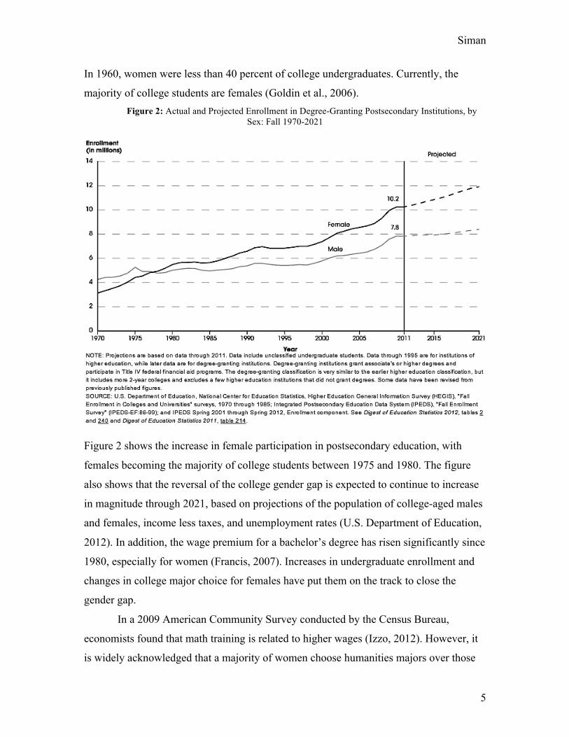
In 1960, women were less than 40 percent of college undergraduates. Currently, the

majority of college students are females (Goldin et al., 2006). Figure 2: Actual and Projected Enrollment in Degree-Granting Postsecondary Institutions, by

Sex: Fall 1970-2021

Figure 2 shows the increase in female participation in postsecondary education, with

females becoming the majority of college students between 1975 and 1980. The figure

also shows that the reversal of the college gender gap is expected to continue to increase

in magnitude through 2021, based on projections of the population of college-aged males

and females, income less taxes, and unemployment rates (U.S. Department of Education,

2012). In addition, the wage premium for a bachelor’s degree has risen significantly since

1980, especially for women (Francis, 2007). Increases in undergraduate enrollment and

changes in college major choice for females have put them on the track to close the

gender gap.

In a 2009 American Community Survey conducted by the Census Bureau,

economists found that math training is related to higher wages (Izzo, 2012). However, it

is widely acknowledged that a majority of women choose humanities majors over those

Siman

6

in math and science. Yet, that majority has been growing smaller since the 1980s. In fact,

females made up about 45 percent of the undergraduate business degrees in 1984-5 and

50 percent by 2001-2, a sharp rise from only 9.1 percent in 1970-1. In addition, since

1970 there have also been increases in the female percentage of bachelor’s degrees in the

life sciences, physical sciences, and engineering disciplines (Francis, 2007). Other than

undergraduate major, another factor that may have a connection to higher earnings is

one’s college GPA, and women have made major strides in that area as well.

In fact, women at undergraduate institutions now outperform men in the

classroom. Studies in Florida and Texas have found that men enroll in fewer credits and

receive lower grades than women during their first semester of college. This persists

until graduation, with male students earning fewer degrees and graduating with lower

GPAs (Conger and Long, 2010). Conger and Long (2010) found that, for example, across

11 public universities in Florida, males graduated with an average of 6.6 fewer credits

than females. In addition, the men had an average GPA 0.2 points lower than the female

average. Both of these results were statistically significant (Conger and Long, 2010).

Despite all of the strides women have made since the 1950’s, especially in the

area of higher education, the gender gap still continues to exist. According to data from

the 1985 Survey of Recent College Graduates, among all those surveyed with a

Bachelor’s Degree, the female contingent earned 18 percent less than the males

(Weinberger, 1998). Thus, in this paper, I delve into the connection between college

experience and wages further by investigating specific features of the undergraduate

academic experience, including major selection and GPA, and the effect they have on

female earnings. Yes, the wage gap has narrowed, but are females with strong grades at a

better advantage? Or does a woman have to pursue traditionally “male-dominated” areas

of study to bridge the wage gap? I explore if the rise of females in business, science, and

math fields is directly linked to an increase in wages for females in their post-graduate

careers. Do females in math, science and engineering majors benefit just as much as

males from choosing a more traditionally rigorous area of study? I investigate whether

the higher performance of women in college actually correlates to an increase in earnings

post graduation, especially in comparison to their male peers who have followed a similar

academic track. I compare the analyses of the earnings in the last year, job type, college

Siman

7

major, and grade point average of the men and women to each other, in order to

determine whether or not a similar academic experience translates into comparable

compensation after graduation. In addition, I compare the females against each other, in

order to reveal whether it is enrollment in what is perceived to be a “difficult” major or a

better academic performance that really makes a difference in future compensation for

women. Finally, I break down the gender pay gap into price and composition effects

based on the theory of the Oaxaca-Blinder Decomposition and various undergraduate

education indicators. The main goal of this investigation is to draw conclusions regarding

whether a female’s choice of major, in addition to strong performance in the classroom,

really does pay off, literally, as much as it does for their male peers.

The paper is organized as follows. Section II reviews the existing literature related

to the link between undergraduate education and the gender pay gap, as well as the

economic theory on the Oaxaca-Blinder Decomposition. Section III describes the

National Longitudinal Survey of Youth, 1997, the dataset used for this analysis. Sections

IV and V present the empirical results, which show the great significance of college

major on the decomposition of the gender pay gap. More specifically, the sections

illustrate that controlling for college major, graduation year, ability, GPA, job industry,

and other demographic indicators can explain a majority of the gender pay gap. Section

VI contains the conclusions I have drawn from these results.

II. Literature Review and Decomposition Framework

The issue of wage differentials in the United States is one that has been studied

widely in economics, whether it be differences based on gender, race, or other factors.

Many researchers have found that by breaking down wage differentials among different

groups using various methodologies, some differences in wages can be explained, while

portions of the differences still remain enigmatic. Huffman and Cohen (2004) found that,

even when employed in like occupations, African American workers in the United States

are paid less than similar white workers. Johnson and Lambrinos (1985) concluded that

there are significant wage differentials between American handicapped workers and non-

handicapped workers, and that these differences are even more pronounced between

males and females. More specifically related to my paper, Blau and Kahn (2004)

Siman

8

investigated the relation between the convergence of the gender pay gap in the 1980’s

and the plateau of the 1990s. They found that there was a “greater negative effect of glass

ceiling barriers on women’s relative wages in the 1990s,” which could possibly reflect

discrimination (Blau and Kahn, 2004). It has been established in economic literature that

wage differences between men and women in the United States exist. This paper will

show whether or not wage differentials between men and women in the same industry are

still significant when broken down by college major and GPA.

Many existing works of economic literature have examined issues related to

female undergraduate choices and employment after graduation, but have not explored

exactly the same themes as my analysis. Goldin, Katz, and Kuziemko (2006) investigate

trends in female enrollment in undergraduate education with data sets from 1957, 1972,

and 1992. They emphasize factors in these changes that differed by gender or were varied

in their consequences. One of these factors is “expectation of future labor force

participation” (Goldin et al., 2006). The authors examine results of the National

Longitudinal Survey of Young Women to address this factor. The survey asked women to

identify whether they expected to be “at work” or “at home, with a family” at age thirty-

five (Goldin et al., 2006). In 1968, between thirty and thirty-five percent chose “at work,”

but by 1979 the number had risen to eighty percent. Delving into this further, the survey

also showed that there existed a fourteen percent difference in college attendance and

completion rates between women who, while in high school, stated they expected to be in

the labor force at age thirty-five and those who did not (Goldin et al., 2006). This reveals

that the reversal of the gap does have to do with female expectations about working after

graduation, and isn’t solely related to changes in social norms or the desire to continue

one’s studies. I do not explore the work expectations of females who have attended

college, but rather the reality of female career choices, including their preparation for

these careers while pursuing their undergraduate degrees. Like Goldin et al., I also use

the National Longitudinal Survey data in my research, and thus, for females, I expect to

see a strong link between undergraduate academic choices and performance and

employment after college in my results. The results are consistent with this view.

Another paper that explores aspects of female undergraduate education is

“Determinants of College Major Choice: Identification Using an Information

Siman

9

Experiment” by Matthew Wiswall and Basit Zafar of the Federal Reserve Bank of New

York (2011). This paper includes an investigation into gender differences in major

choice. Specifically, the authors examine the differences between male and female

students’ perception of average earnings within different fields. Wiswall and Zafar found

that beliefs about future relative major choices are positively and strongly associated with

beliefs about future self-earnings. However, this factor was a substantially smaller

determinant in women than in men. The authors found that, to women, ability in the field

was a much more important factor in choosing their major. This raises the question of

whether the women who choose math, science and other business-related majors have

higher abilities in these fields than their male counterparts. In addition, the paper

examined the difference between male and female perception of earnings after majoring

in different fields. An interesting result was that both males and females overestimated

female full-time earnings after majoring in Economics and business fields by about thirty

percent (Wiswall and Zafar, 2011). This finding suggests that perhaps women in these

fields do not earn as much as their male peers. I will not be investigating the reasons why

women and men choose different majors or their perceptions of future earnings; instead, I

will show the connection between their major choices and actual earnings. My research

will determine whether Wiswall and Zafar’s findings about female earnings are true

across datasets, or whether females who major in Economics and business fields choose

jobs in different industries than males, thus explaining the difference between perceptions

of earnings and reality. My thesis will also show if the difference has any link to

academic performance while in college.

Zafar (2013) also investigated the factors which lead males and females to choose

their college majors in even more depth. Results of a study of sophomores at

Northwestern University showed that the most important determinants of major choice

were enjoying classwork, enjoying work at future jobs, and parental approval. A very

interesting result of Zafar’s study is that non-monetary reasons account for 75 percent of

choice behavior for females, but only account for 45 percent of choice behavior for

males. These preferences extend into the workplace (Zafar, 2013). My dataset will not be

limited to graduates of prestigious colleges such as Northwestern University, but I will be

able to observe differences in major choice between females and males who have

Siman

10

demonstrated similar abilities in standardized tests. In addition, Zafar’s research makes it

apparent that accounting for job industry selection will be important to my investigation

of the link between college academic experience and earnings.

The paper “Why are Men Falling Behind? Gender Gaps in College Performance

and Persistence,” mentioned during the Introduction, by Dylan Conger and Mark C. Long

(2010) is also useful to examine. The authors study the disparity between male and

female college performance. They find that women on average earn more credits, higher

grades, and are more likely to graduate. However, the investigation also reveals that

much of this difference can be explained by chosen area of study; females tend to choose

“easier” majors than males (Conger and Long, 2010). Thus, the paper suggests that

college major choice is a more important determinant of future earnings than GPA. Like

Conger and Long, I will be comparing the GPAs of males and females, however, I focus

on math, science, and business fields, and link the GPAs to future earnings. By

examining both the subject’s major choice and GPA’s effect on earnings, my research

will reveal whether the females who do not choose “easy” humanities tracks do make as

much as men with similar educational backgrounds.

Hamermesh and Donald (2004) also address the link between college experience

and income. Their paper provides a detailed examination of undergraduate major, course

selection, grades in these courses, and subsequent earnings twenty years post-graduation.

Hamermesh and Donald found that the highest-earning majors (Honors and “hard”

business majors) averaged almost three times that of the lowest (Education), and that the

fraction of women in the highest-earning majors was lower than in the lowest-earning

majors. Another interesting result of the study was that the adjusted female wage gap for

single women compared to single men is only eight percent, while the adjusted gap

between married women and married men is twenty-five percent. The authors also noted

that within a major (results for both males and females combined), going from a B to A

average GPA raised annual earnings by about seven percent (Donald and Hamermesh,

2004). My research will be similar in investigating the effects of major choice and GPA

on earnings, however, I am more specifically looking at the differences in these effects

between males and females. It is important to use my research to extend the results of this

Siman

11

study further to note whether the highest-earning females pursued more difficult areas of

study and/or earned higher grades.

Another source that is relevant to my investigation is the paper “Gender

Differences in Executive Compensation and Job Mobility” by George-Levi Gayle, Limor

Golan, and Robert A. Miller. This paper is especially interesting because it focuses on

women who have reached executive level positions. The authors examine compensation

data with background characteristics, including education. The results showed that,

conditional on survival as an executive, women have a higher probability of becoming

CEO. However, average career compensation was lower for female executives than for

male executives (Gayle et al., 2012). My research shows whether or not females who

have chosen a rigorous area of study and remain in the work force as long as their male

counterparts receive the same return in in income.

In 2010, Lin published the paper “Gender Wage Gaps by College Major in

Taiwan: Empirical Evidence from the 1997-2003 Manpower Utilization Survey.” This

paper contains a very similar purpose to my investigation, but uses data from Taiwan

rather than the United States. When observing overall gender gaps by college major, the

results showed that Agriculture, Literature, and other similar majors had smaller gender

pay gaps, while Medicine and Business showed the largest gaps. In addition, the gender

pay gaps were statistically significant in the majors of Education, Engineering, Law,

Business, and Medicine. However, Lin found that controlling for college major with

dummy variables increases the proportion of the price effect (also known as the

characteristic effect) in the Oaxaca-Blinder Decomposition, meaning that individual

characteristics became more important to wages than whether the individual was a male

or female. He also discovered that when investigating the gender pay gap by occupation

industry, wage differences were “statistically negligible” in all majors except for

medicine (Lin, 2010). Still, some differences did exist between male and female pay after

majoring in certain fields. Education, Law, Business, and Engineering demonstrated a

gender pay gap that slightly favored males, while Literature, Education, and, surprisingly,

Science majors demonstrated a pay gap that actually favored females. Thus, it will be

important in my research to also break down the gender pay gap by job industry and type,

as well as major. I use the methodology of this paper, which applied a pooled Neumark

Siman

12

estimator to the Oaxaca-Blinder Decomposition, to help guide me through my research.

However, Lin’s paper focuses on the gender gap within a major, while mine also

addresses the gap across majors.

Previous economists, including Lin, have studied the effects of multiple variables

on wages by applying the Neumark estimator to implement the Oaxaca-Blinder

Decomposition. The Oaxaca-Blinder Decomposition attempts to decompose outcomes (in

this case, earnings) into price and decomposition effects. Using this theory, one is able to

break down the “price effect” and the “composition effect” on average wages. The

Neumark estimator was introduced by David Neumark (1988) as a method to build a

wage structure that is nondiscriminatory, but that is based on the discriminatory tastes of

employers. Neumark assumed that the utility function for discriminatory tastes of

employers within a certain type of labor (skilled, unskilled) is homogenous of degree zero

with respect to labor inputs from each of the genders. With this assumption in mind, he

found that the nondiscriminatory wage structure is the coefficient vector of the wage

regression equation over the pooled sample, and, thus, can be represented as a weighted

average. Hence, weighted-average earnings can be used to derive the Oaxaca-Blinder

Decomposition (Neumark, 1988). The average wage for a gender is the weighted average

of the wages the gender earns in each occupation. The weights are the share of workers of

a given gender within each occupation. Roughly speaking, in a general application of the

Oaxaca-Blinder Decomposition, the price effect has to do with wage differentials across

genders for certain occupations, and the composition effect is related to differences in

occupational choice between males and females. In my paper, I separate the differences

in mean wages between males and females into those attributed to individual

characteristics (the “price effect”) and the component associated with the differences in

the characteristics themselves (the “composition effect”). To be more specific, the price

effect I am investigating is: given a specific major or GPA, what are the differences in

wages between males and females. The composition effect would be something along the

lines of: females in general tend to have lower wages because they tend to choose

humanities majors over math, science, and business fields. My results quantify both the

composition and price effect.

Siman

13

Utilizing the background information found in the aforementioned sources, plus

the results of further research, I investigate the undergraduate college experience for

women and its connections to the narrowing of the gender pay gap. Unlike much of the

current literature, I do not focus on solely female choices and results in undergraduate

academics, but instead connecting these to their lives after graduation. Similar research

on the link between academic decisions while in college and earnings has been done, but

it does not specifically address this link’s effect on the gender pay gap, or the research

does not use data from the United States. I do not examine how the gap has changed over

time, rather, I paint a picture of the gap relative to the college experience as it exists

today.

III. Data

The dataset I have chosen to accomplish my goals part of a broad U.S.

government initiative known as the National Longitudinal Surveys. The National

Longitudinal Surveys are a set of surveys conducted by the Bureau of Labor Statistics.

These surveys have gathered data on the labor market activities and special life events

(marriage, childbirth, etc.) of multiple groups of men and women in the United States.

The surveys have been conducted for over four decades, beginning with the National

Longitudinal Surveys of Young Men and Older Men in 1966 (Bureau of Labor Statistics,

2011). The survey that I use in my research is the National Longitudinal Survey of Youth

1997.

The National Longitudinal Survey of Youth 1997, or NLSY97, surveyed a

nationally representative sample of approximately 9,000 people in the United States who

were between the ages of 12 and 16 on December 31, 1996. The first round of the survey

was conducted in 1997, in which the young people and their parents participated in hour-

long individual interviews. This round also included a questionnaire revealing each

youth’s demographic information as well as family background and history. The youths

continue to be interviewed annually about educational and labor market experience, as

well as other personal relationship and life events (Bureau of Labor Statistics, 2011). The

NLSY97 data contains numerous variables which are essential to my research.

Siman

14

The NLSY97 measured detailed information on both the subjects’ educational and

employment experience. Employment data includes occupation, industry, hours, overtime

hours, previous year’s income from wages or salary, benefits available at employer, and

general job satisfaction. Some of the educational variables measured are type of college

attended (2-year, 4-year, public, or private), cost of attendance at the college, type and

amount of educational loans and financial aid, type of degree received, field of study in

each term, and grade point average in each term. Other variables that could be interesting

to observe are current marital status, number, sex, and ages of children, and fertility

expectations. And, of course, all surveyed do have to disclose their gender (Bureau of

Labor Statistics, 2011). Thus, the NLSY97 does include all the variables that I need to

conduct my research. However, the dataset does not specify exactly which undergraduate

institution the subjects attended, thus, I was unable to control for the academic rigor of

the college. Yet, the dataset does contain some proxies for ability measures, such as

Armed Forces Qualification Test results. All in all, the NLSY97 is a very detailed dataset

and is more than sufficient to complete my investigation.

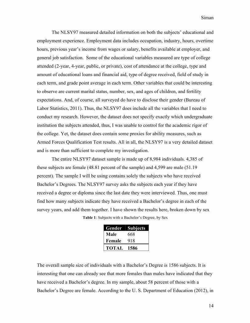
The entire NLSY97 dataset sample is made up of 8,984 individuals. 4,385 of

these subjects are female (48.81 percent of the sample) and 4,599 are male (51.19

percent). The sample I will be using contains solely the subjects who have received

Bachelor’s Degrees. The NLSY97 survey asks the subjects each year if they have

received a degree or diploma since the last date they were interviewed. Thus, one must

find how many subjects indicate they have received a Bachelor’s degree in each of the

survey years, and add them together. I have shown the results here, broken down by sex Table 1: Subjects with a Bachelor’s Degree, by Sex

The overall sample size of individuals with a Bachelor’s Degree is 1586 subjects. It is

interesting that one can already see that more females than males have indicated that they

have received a Bachelor’s degree. In my sample, about 58 percent of those with a

Bachelor’s Degree are female. According to the U. S. Department of Education (2012), in

Gender Subjects Male 668 Female 918 TOTAL 1586

Siman

15

2009-10, females earned approximately 57 percent of Bachelor’s Degrees. Thus, my

sample is consistent with national trends. Yet, looking at the specific Stata results, the

data does show that many subjects stopped being interviewed during each round,

especially during the later years. Thus, there may be some sample selection bias here.

Next, the sample was broken down further by college major. The NLSY97 asks

subjects enrolled in college whether they are majoring in 1 of 37 different areas. Those

which I include in my investigation as business, science, or math fields are: Biological

Sciences, Business Management, Computer/Information Science, Economics,

Engineering, Mathematics, and Physical Sciences. The NLSY97 data does not have a

specific indicator for the major that the subjects receive their Bachelor’s Degree in.

Rather, each year, the survey asks each subject to indicate their major during each term

since they were last interviewed. Thus, I created my own variable by specifying each

individual’s major indicator in the year in which they received their Bachelor’s Degree,

matching using the subject’s identification number. The results are shown in the

following table, separated by sex. Table 2: College Major upon Graduation, by Sex

Major Males Females Percent of STEMB Total

Biological Sciences 27 44 11.04 Business Management 165 171 52.26 Computer Science 55 12 10.42 Economics 36 16 8.09 Engineering 59 21 12.44 Mathematics 12 8 3.11 Physical Sciences 8 9 2.64 TOTAL 362 281

The overall sample size for subjects in Math, Science, and Business related

majors is 643 subjects, 362 male and 281 female. Thus, one can already see that,

although more females in the sample received Bachelor’s Degrees than males, less

majored in these areas. Only 43.7 percent of STEMB majors are female. Also, overall,

the STEMB majors make up approximately 41 percent of the sample. Interestingly, there

are more females in the sample who majored in the Biological Sciences and Business

Siman

16

Management than males. However, much fewer women majored in

Computer/Information Sciences, Economics, and Engineering.

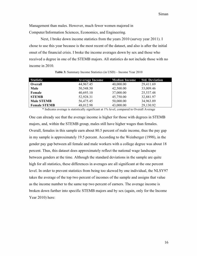
Next, I broke down income statistics from the years 2010 (survey year 2011). I

chose to use this year because is the most recent of the dataset, and also is after the initial

onset of the financial crisis. I broke the income averages down by sex and those who

received a degree in one of the STEMB majors. All statistics do not include those with no

income in 2010. Table 3: Summary Income Statistics (in USD) – Income Year 2010

Statistic Average Income Median Income Std. Deviation Overall 44,967.45 40,000.00 29,411.69 Male 50,548.50 42,500.00 33,009.46 Female 40,693.10 37,000.00 25,537.48 STEMB 52,928.31 45,750.00 32,881.97 Male STEMB 56,475.45 50,000.00 34,963.89 Female STEMB 48,012.98 43,000.00 29,130.92

* Indicates average is statistically significant at 1% level, compared to Overall Average

One can already see that the average income is higher for those with degrees in STEMB

majors, and, within the STEMB group, males still have higher wages than females.

Overall, females in this sample earn about 80.5 percent of male income, thus the pay gap

in my sample is approximately 19.5 percent. According to the Weinberger (1998), in the

gender pay gap between all female and male workers with a college degree was about 18

percent. Thus, this dataset does approximately reflect the national wage landscape

between genders at the time. Although the standard deviations in the sample are quite

high for all statistics, these differences in averages are all significant at the one percent

level. In order to prevent statistics from being too skewed by one individual, the NLSY97

takes the average of the top two percent of incomes of the sample and assigns that value

as the income number to the same top two percent of earners. The average income is

broken down further into specific STEMB majors and by sex (again, only for the Income

Year 2010) here:

Siman

17

Table 4: Average Income by STEMB Major and Sex – Income Year 2010

Major Overall Average

Male Average

Female Average

Biological Sciences 45,869.32 45,383.18 46,183.88 Business Management 49,625.62 54,018.56 44,884.03

Computer Science 57,145.84 55,330.84 66,901.50 Economics 54,356.44 62,296.63 35,300.00

Engineering 69,881.14 70,606.90 67,894.84 Mathematics 48,441.29 43,590.91 57,333.67

Physical Sciences 46,616.88 44,142.86 48,541.11

Examining these numbers shows an interesting trend, the female average is higher than

the male average income in about half of these STEMB majors. Thus, it is necessary to

break down these results even further to determine where the root of the pay gap lies.

IV. Empirical Specification: Preliminary Results

In “Gender Wage Gaps by College Major in Taiwan: Empirical Evidence from

the 1997-2003 Manpower Utilization Survey,” Lin applied methodology that I emulate

with my investigation, using the pooled Neumark estimator to implement the Oaxaca-

Blinder Decomposition. He begins by considering a standard log-wage model:

𝑦! = ∝!+ 𝑥! 𝜃! + 𝛽!!𝑑!" + 𝜋!

!𝑞!" + 𝜀! ;!

!!!

!

!!!

𝑖 = 1, . . . ,𝐹; 𝑗 = 1, . . . , 𝐽; 𝑘 = 1, . . . ,𝐾; (1)

𝑦! = ∝!+ 𝑥! 𝜃! + 𝛽!!𝑑!" + 𝜋!!𝑞!" + 𝜀! ;!

!!!

!

!!!

𝑖 = 1, . . . ,𝑀; 𝑗 = 1, . . . , 𝐽; 𝑘 = 1, . . . ,𝐾; (2)

where equations (1) and (2) represent the log-wage regressions, respectively, for F female

and M male workers. In the equation, yi is the log of the hourly wage, xi is a vector of

continuous characteristic regressors, and dij is a dummy variable equal to one if the ith

worker’s field of study is the jth major, and zero otherwise. The qik captures other sets of

dummy variables (Lin, 2010). The next step is to average the fitted values in equations

Siman

18

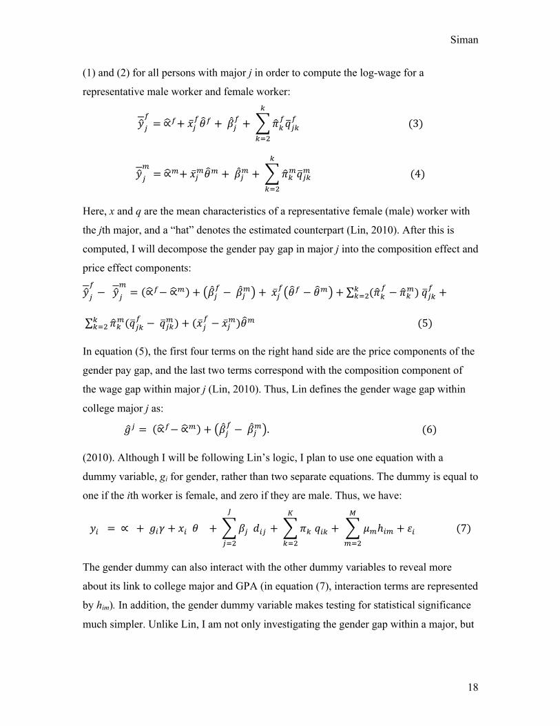
(1) and (2) for all persons with major j in order to compute the log-wage for a

representative male worker and female worker:

𝑦!!= ∝!+ 𝑥!

!𝜃! + 𝛽!! + 𝜋!

!𝑞!"!

!

!!!

(3)

𝑦!!= ∝!+ 𝑥!!𝜃! + 𝛽!! + 𝜋!!𝑞!"!

!

!!!

(4)

Here, x and q are the mean characteristics of a representative female (male) worker with

the jth major, and a “hat” denotes the estimated counterpart (Lin, 2010). After this is

computed, I will decompose the gender pay gap in major j into the composition effect and

price effect components:

𝑦!!− 𝑦!

!= ∝!− ∝! + 𝛽!

! − 𝛽!! + 𝑥!! 𝜃! − 𝜃! + (𝜋!

! − 𝜋!!) 𝑞!"!!

!!! +

𝜋!!(𝑞!"!!

!!! − 𝑞!"!)+ (𝑥!! − 𝑥!!)𝜃! (5)

In equation (5), the first four terms on the right hand side are the price components of the

gender pay gap, and the last two terms correspond with the composition component of

the wage gap within major j (Lin, 2010). Thus, Lin defines the gender wage gap within

college major j as:

𝑔! = ∝!− ∝! + 𝛽!! − 𝛽!! . (6)

(2010). Although I will be following Lin’s logic, I plan to use one equation with a

dummy variable, gi for gender, rather than two separate equations. The dummy is equal to

one if the ith worker is female, and zero if they are male. Thus, we have:

𝑦! = ∝ + 𝑔!𝛾 + 𝑥! 𝜃 + 𝛽! 𝑑!" + 𝜋! 𝑞!" + 𝜇!ℎ!"

!

!!!

+ 𝜀!

!

!!!

!

!!!

(7)

The gender dummy can also interact with the other dummy variables to reveal more

about its link to college major and GPA (in equation (7), interaction terms are represented

by him). In addition, the gender dummy variable makes testing for statistical significance

much simpler. Unlike Lin, I am not only investigating the gender gap within a major, but

Siman

19

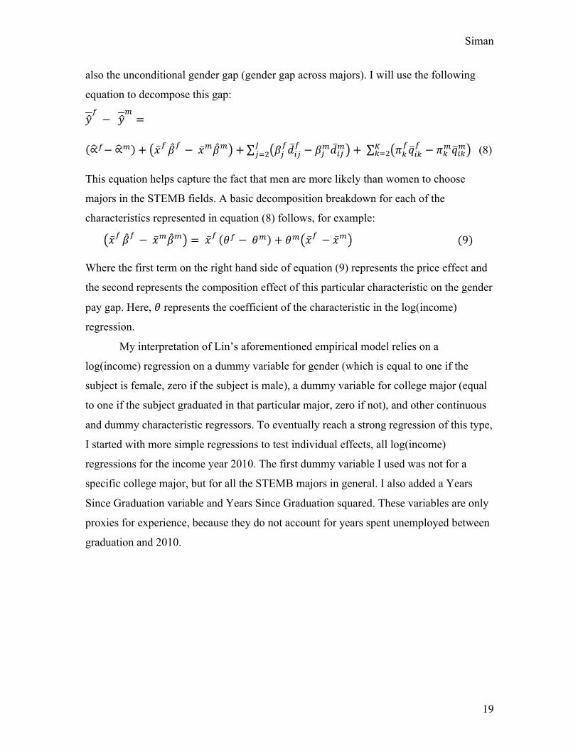
also the unconditional gender gap (gender gap across majors). I will use the following

equation to decompose this gap:

𝑦!− 𝑦

!=

∝!− ∝! + 𝑥!𝛽! − 𝑥!𝛽! + 𝛽!!𝑑!"

! − 𝛽!!𝑑!"!!!!! + 𝜋!

!𝑞!"! − 𝜋!!𝑞!"!!

!!! (8)

This equation helps capture the fact that men are more likely than women to choose

majors in the STEMB fields. A basic decomposition breakdown for each of the

characteristics represented in equation (8) follows, for example:

𝑥!𝛽! − 𝑥!𝛽! = 𝑥! 𝜃! − 𝜃! + 𝜃! 𝑥! − 𝑥! (9)

Where the first term on the right hand side of equation (9) represents the price effect and

the second represents the composition effect of this particular characteristic on the gender

pay gap. Here, 𝜃 represents the coefficient of the characteristic in the log(income)

regression.

My interpretation of Lin’s aforementioned empirical model relies on a

log(income) regression on a dummy variable for gender (which is equal to one if the

subject is female, zero if the subject is male), a dummy variable for college major (equal

to one if the subject graduated in that particular major, zero if not), and other continuous

and dummy characteristic regressors. To eventually reach a strong regression of this type,

I started with more simple regressions to test individual effects, all log(income)

regressions for the income year 2010. The first dummy variable I used was not for a

specific college major, but for all the STEMB majors in general. I also added a Years

Since Graduation variable and Years Since Graduation squared. These variables are only

proxies for experience, because they do not account for years spent unemployed between

graduation and 2010.

Siman

20

Table 5: Log(Income) Regression on Gender, STEMB, Years since Graduation, Years since Grad Squared

Variables Coefficients (Robust Std. Errors) P-value

Regression Constant R-squared

Gender -0.182 0.000*** 9.951 0.1014 (0.0427)

STEMB Major 0.280 0.000*** - - (0.0430)

Years Since 0.116 0.005*** - - Graduation (0.0410)

Years Since -0.003 0.410 - - Graduation Squared (0.0038)

*;**;*** represent statistically significant at the 10%, 5%, 1% levels respectively

Gender here is a statistically significant variable, showing that between two people with

degrees in a STEMB major who graduated in the same year, but of the opposite sex, the

female still earns over 18 percent less than the male. Additionally, having a degree in a

STEMB major increases earnings by approximately 28 percent, a very large, and

statistically significant, number. This regression also shows that for two people of the

same gender with degrees in a STEMB major, an additional year of work experience adds

over 11 percent to income.

To include more controls for ability in order to isolate the true effect of gender on

income, I added the AFQT variable to my analysis. The AFQT (Armed Forces

Qualification Test) is a measure of intellectual ability, in both verbal reasoning and math,

which is scored in the range of 0 to 100. Controlling for AFQT also helps to control for

selection unobservables because it captures some of the ability bias. The variable

included in the following regression indicates the percentile that the subject’s AFQT

score placed them in.

Siman

21

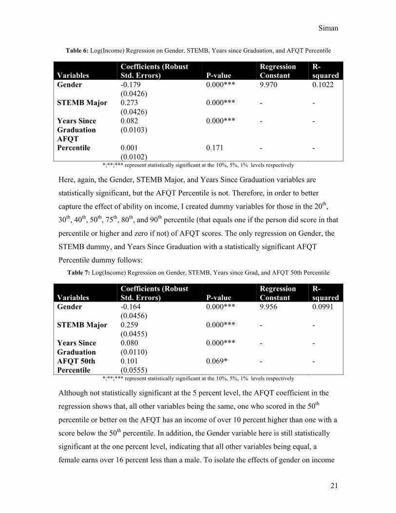
Table 6: Log(Income) Regression on Gender, STEMB, Years since Graduation, and AFQT Percentile


Regression Constant

R-squared

Gender -0.179 0.000*** 9.970 0.1022 (0.0426)

STEMB Major 0.273 0.000*** - - (0.0426)


AFQT Percentile 0.001 0.171 - - (0.0102)


Here, again, the Gender, STEMB Major, and Years Since Graduation variables are

statistically significant, but the AFQT Percentile is not. Therefore, in order to better

capture the effect of ability on income, I created dummy variables for those in the 20th,

30th, 40th, 50th, 75th, 80th, and 90th percentile (that equals one if the person did score in that

percentile or higher and zero if not) of AFQT scores. The only regression on Gender, the

STEMB dummy, and Years Since Graduation with a statistically significant AFQT

Percentile dummy follows: Table 7: Log(Income) Regression on Gender, STEMB, Years since Grad, and AFQT 50th Percentile


Regression Constant

R-squared

Gender -0.164 0.000*** 9.956 0.0991 (0.0456)

STEMB Major 0.259 0.000*** - - (0.0455)


AFQT 50th 0.101 0.069* - - Percentile (0.0555)


Although not statistically significant at the 5 percent level, the AFQT coefficient in the

regression shows that, all other variables being the same, one who scored in the 50th

percentile or better on the AFQT has an income of over 10 percent higher than one with a

score below the 50th percentile. In addition, the Gender variable here is still statistically

significant at the one percent level, indicating that all other variables being equal, a

female earns over 16 percent less than a male. To isolate the effects of gender on income

Siman

22

within specific college majors, I next grouped some of the majors together in order to

create larger sample sizes, and then performed regressions similar to the regression in

Table 7. The major groups are Business/Economics, Hard Sciences/Math, Computer

Science, and Engineering. For each one, I regressed log (income) on Gender, the major

group dummy (equal to one if the subject has a degree in that group, zero if not), Years

since Graduation, and each of the AFQT Percentile dummies. The regressions that follow

are those with statistically significant AFQT dummies of the highest percentile for each

major group. Table 8: Log(Income) Reg on Gender, Business/Econ Major, Years since Grad, AFQT 80th Percentile


Regression Constant

R-squared

Gender -0.202 0.000*** 10.072 0.0828

(0.0455)

Business/Econ 0.167 0.001*** - - Major (0.0491)


AFQT 80th 0.094 0.050** - - Percentile (0.0478)


This regression shows that for a female Business or Economics major who graduated in

the same year as a male, both with AFQT scores in the 80th percentile, the female earns

over 20 percent less than the male counterpart, a very big difference for two people of

very similar credentials and ability. Table 9: Log(Income) Reg on Gender, Engineering Major, Years since Grad, AFQT 50th Percentile


Regression Constant

R-squared

Gender -0.196 0.000*** 10.048 0.0895 (0.0455)

Engineering 0.404 0.000*** - - Major (0.0876)




Siman

23

The results for Engineering majors are less descriptive, because the AFQT 50th percentile

variable was the highest percentile for which results were statistically significant, but still

indicate that a female engineer who graduated in the same year as a male engineer, both

with AFQT scores in the top 50 percent, earns almost twenty percent less. Table 10: Log(Income) Reg on Gender, CompSci Major, Years since Grad, AFQT 80th Percentile


Regression Constant

R-squared

Gender -0.205 0.000*** 10.102 0.0777 (0.0464)

Computer 0.212 0.032** - - Science Major (0.0987)




This regression reveals very similar results, regarding gender, to the Business/Economics

regression (Table 8). For a female Computer Science major who graduated in the same

year as a male, both with AFQT scores in the 80th percentile, the female earns over 20

percent less than the male counterpart, again, a large disparity for two people of similar

educational and ability backgrounds. Table 11: Log(Income) Reg on Gender, Science/Math Major, Years since Grad, AFQT 80th Percentile


Regression Constant

R-squared

Gender -0.242 0.000*** 10.133 0.0763 (0.0428)

Hard Sciences/ 0.030 0.692 - - Math Major (0.0754)




Interestingly, here the Hard Sciences/Math group major dummy is not statistically

significant. The Gender variable is though, and shows that for female majors in this

group, all else being equal (graduation year, AFQT score above or below the 80th

percentile), incomes tend to be about 24 percent lower. Together, all of the

Siman

24

aforementioned regressions show that the effect of Gender on income is both large in

magnitude, and statistically significant, ranging from about negative 16 to 20 percent.

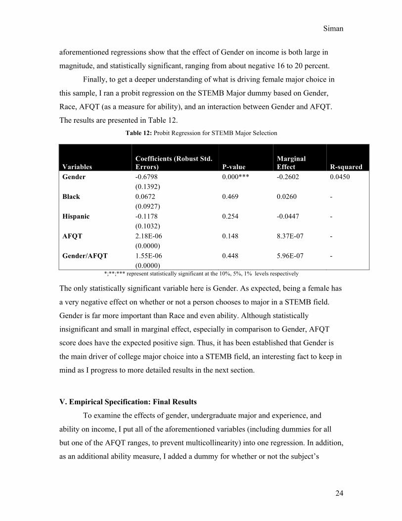
Finally, to get a deeper understanding of what is driving female major choice in

this sample, I ran a probit regression on the STEMB Major dummy based on Gender,

Race, AFQT (as a measure for ability), and an interaction between Gender and AFQT.

The results are presented in Table 12. Table 12: Probit Regression for STEMB Major Selection


Marginal Effect R-squared

Gender -0.6798 0.000*** -0.2602 0.0450 (0.1392)

Black 0.0672 0.469 0.0260 - (0.0927)

Hispanic -0.1178 0.254 -0.0447 - (0.1032)

AFQT 2.18E-06 0.148 8.37E-07 - (0.0000)

Gender/AFQT 1.55E-06 0.448 5.96E-07 - (0.0000)


The only statistically significant variable here is Gender. As expected, being a female has

a very negative effect on whether or not a person chooses to major in a STEMB field.

Gender is far more important than Race and even ability. Although statistically

insignificant and small in marginal effect, especially in comparison to Gender, AFQT

score does have the expected positive sign. Thus, it has been established that Gender is

the main driver of college major choice into a STEMB field, an interesting fact to keep in

mind as I progress to more detailed results in the next section.

V. Empirical Specification: Final Results

To examine the effects of gender, undergraduate major and experience, and

ability on income, I put all of the aforementioned variables (including dummies for all

but one of the AFQT ranges, to prevent multicollinearity) into one regression. In addition,

as an additional ability measure, I added a dummy for whether or not the subject’s

Siman

25

cumulative college GPA was a 3.0 or above (equal to one if so, zero if not) and an

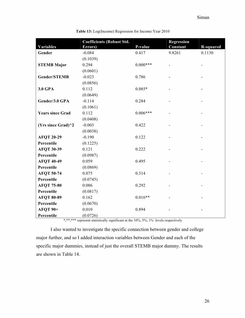
interaction term between Gender and this dummy. The results are shown in Table 13.

In this regression, the STEMB major coefficient is statistically significant and of

very high magnitude, STEMB majors make almost 30 percent more than non-STEMB

majors. The 3.0 GPA coefficient is also statistically significant at the 10 percent level and

indicates that having a GPA of 3.0 or higher raises income by over 11 percent. The Years

Since Graduation variable is also statistically significant and of the expected sign.

The interaction terms, although not statistically significant, have interesting point

estimates. The Gender and STEMB major interaction has a very small magnitude, which

suggests that both females and males have the same return for majoring in a STEMB

field. On the other hand, the Gender and 3.0 GPA dummy interaction has a higher

magnitude than the GPA dummy itself and is in the opposite direction. This indicates that

females receive no return from earning a high GPA, whereas males see a jump in their

income.

Most importantly, note that the Gender coefficient is now statistically

insignificant, and has decreased in magnitude to show that females earn only 8 percent

less than males. This result suggests that, when majoring in a STEMB field, GPA, Years

since Graduation, and AFQT ability measures are controlled for, only about 8 percent of

the gender pay gap remains unexplained.

Siman

26

Table 13: Log(Income) Regression for Income Year 2010



Gender -0.084 0.417 9.8261 0.1130 (0.1039)

STEMB Major 0.294 0.000*** - - (0.0601)

Gender/STEMB -0.023 0.786 - - (0.0856)

3.0 GPA 0.112 0.085* - - (0.0649)

Gender/3.0 GPA -0.114 0.284 - - (0.1061)

Years since Grad 0.112 0.006*** - - (0.0408)

(Yrs since Grad)^2 -0.003 0.422 - - (0.0038)

AFQT 20-29 -0.190 0.122 - - Percentile (0.1225)

AFQT 30-39 0.121 0.222 - - Percentile (0.0987)

AFQT 40-49 0.059 0.495 - - Percentile (0.0869)

AFQT 50-74 0.075 0.314 - - Percentile (0.0745)

AFQT 75-80 0.086 0.292 - - Percentile (0.0817)

AFQT 80-89 0.162 0.016** - - Percentile (0.0670)

AFQT 90+ 0.010 0.894 - - Percentile (0.0726)


I also wanted to investigate the specific connection between gender and college

major further, and so I added interaction variables between Gender and each of the

specific major dummies, instead of just the overall STEMB major dummy. The results

are shown in Table 14.

Siman

27



Regression Constant

R-squared

Gender -0.097 0.346 9.832 0.1220 (0.1039)

Business/Econ 0.268 0.000*** - - (0.0687)

Gender/Business -0.048 0.622 - - (0.0974)

Engineering 0.447 0.000*** - - (0.1179)

Gender/Engineering 0.252 0.121 - - (0.1623)

Hard Sciences 0.085 0.397 - - (0.1009)

Gender/Hard Sciences 0.086 0.567 - - (0.1509)

Computer Science 0.250 0.025** - - (0.1109)

Gender/CompSci 0.401 0.057* - - (0.2102)

3.0 GPA 0.114 0.077* - - (0.0643)

Gender/3.0 GPA -0.109 0.299 - - (0.1051)

Years since Grad 0.116 0.005*** - - (0.0409)

(Yrs since Grad)^2 -0.003 0.370 - - (0.0038)

AFQT 20-29 -0.190 0.124 - - Percentile (0.1232)

AFQT 30-39 0.118 0.238 - - Percentile (0.1002)

AFQT 40-49 0.053 0.543 - - Percentile (0.0871)

AFQT 50-74 0.077 0.305 - - Percentile (0.0748)

AFQT 75-80 0.082 0.315 - - Percentile (0.0817)

AFQT 80-89 0.160 0.018** - - Percentile (0.0681)

AFQT 90+ -0.002 0.981 - - Percentile (0.0729)


Siman

28

In this regression, all of the STEMB major coefficients are statistically significant, except

for the hard sciences and math coefficient. All of the majors have the expected sign and

magnitude, with Engineers having the highest return on their choice of major, increasing

wages by almost 45 percent. The 3.0 GPA dummy variable is statistically significant at

the 10 percent level, with having a GPA of 3.0 or higher increasing wages by about 11

percent. The Years since Graduation and Years since Graduation squared variables have

the expected signs, and the statistically significant Years since Graduation variable

indicates that each year out of college, a proxy for each year of experience, adds almost

12 percent to one’s wages. The AFQT variables are not statistically significant except for

the 80th to 89th percentile. Finally, note that with the addition of all of the interaction

coefficients, the gender variable is no longer statistically significant. However, it still has

a negative sign and a magnitude of 0.097, suggesting that about 10 percent of the gender

pay gap remains unexplained.

Examining the interaction coefficients offers more insight into the connection

between the gender pay gap and college experience. The only interaction coefficient that

is statistically significant at the 10 percent level or better is the Gender and Computer

Science major interaction. Still, it is interesting to note that the only college major and

gender interaction that is negative is for the Business and Economics majors. Thus, the

results suggest that for the STEMB majors, with the exception of the business group,

females actually have a higher proportionate return for choosing this major than males.

However, taking into account the negative Gender dummy coefficient of -0.097, the

return is not as high as the interaction coefficients suggest.

The last interaction variable to note is the Gender and 3.0 GPA dummy

interaction variable. Although it is not statistically significant, it is negative and of almost

the exact opposite magnitude as the 3.0 GPA dummy alone. This suggests, especially

when taken into account with the negative coefficient of the Gender dummy, that, all else

being equal, females do not see the same return of a GPA above 3.0 in their future

income that their male classmates do.

A key takeaway from the regression results in Table 14 is that once experience,

AFQT, GPA, and college major has been controlled for, the Gender coefficient changes

dramatically from that in the earlier regressions. Firstly, it becomes statistically

Siman

29

insignificant. Secondly, compared to the earlier results, the gender effect falls by about a

half to a third, as measured by the point estimates. This suggests that controlling for these

factors renders Gender unimportant.

Now that the effects of gender, experience, and ability on income have been

isolated by major and examined, I put together all of these variables, along with other

important demographic and industry indicators, into one log(income) regression. The first

new addition is a dummy for whether or not the subject has a child (equal to one if they

have one or more children, zero if they have not). Another dummy variable included is

one for marital status, one if the subject is married or lives with a significant other, zero if

not. I also added individual dummies for the Black and Hispanic race indicators. There is

some ambiguity in the possible indications of race available in the NLSY97 survey (the

only options are Black, Hispanic, Mixed Race (Non-Black/Non-Hispanic), or Non-

Black/Non-Hispanic), which leaves some racial groups without a clear classification.

Thus, isolating the Black and Hispanic options will make the results more clear and easy

to interpret. I also felt that it was important to isolate the effects of job industry on

income. The industries I have isolated are the Finance/Insurance industry, Education,

Manufacturing, and Retail industries. I wanted to delve into the issue of gender further by

adding some family life interaction variables as well. Therefore, I created interaction

terms (with the values multiplied together as the interaction) for the Gender and Child

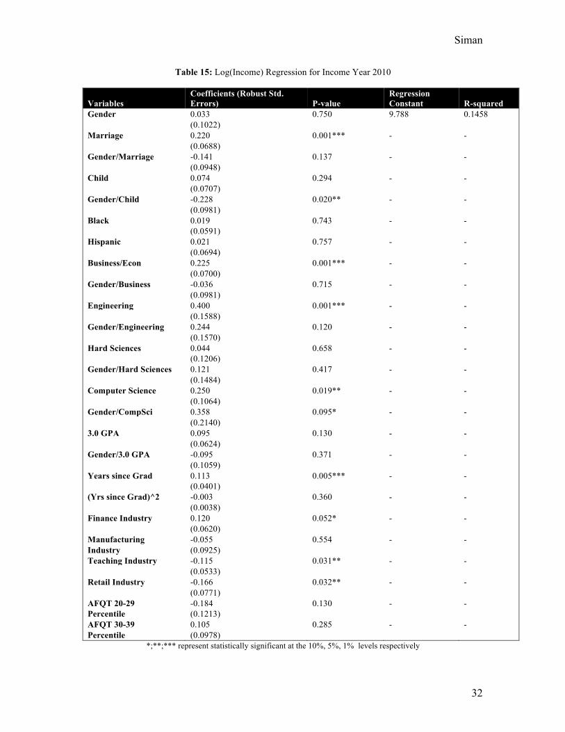
dummies and the Gender and Marital Status dummies. The results of this regression are

in Table 15.

Interestingly, the child and race dummies are not statistically significant, and have

very small coefficients. The small coefficients of the race dummies can potentially be

explained by the fact all subjects do have a bachelor’s degree, and the child dummy could

be a result of including an interaction between Child and Gender. A male with a child is

likely to work to earn more money to support that child, while a female may leave the

workforce, and these effects could be offsetting each other. The coefficient for the

Gender and Child interaction term in the regression shows that having a child has a

highly negative impact on earnings for females. About 32 percent of females in my

sample have children, so this interaction term is not picking up the effects of the gender

variable. The large magnitude of the Gender and Child interaction is consistent with the

Siman

30

findings of Waldfogel (1998), who determined that the wage gap between females with

children and males without was almost 27 percent in 1994. On the other hand, the marital

status dummy is statistically significant, but the interaction term is not. The magnitude of

the marital status dummy is very large, suggesting that, all else being equal, a married

man earns 20 percent more than an unmarried man. Although the interaction term isn’t

significant, it’s negative sign indicates that this effect is offset quite a bit if the subject is

a woman. This is consistent with the findings of Donald and Hamermesh (2004), who

found that the wage gap between a single man and woman is significantly less than that

between a married man and a married woman. Nonetheless, all of these variables show

that family choices, rather than discrimination against women, have a very large impact

on income.

The major group coefficients are similar to those in the earlier results presented in

Table 14. All of the STEMB major dummies have positive coefficients, with

Engineering, unsurprisingly, with the highest magnitude. All but the Hard Sciences group

are statistically significant at the 5 percent level or better. Engineering majors earn about

40 percent more than non-Engineers, all else being equal. Although they are not

statistically significant, examining the magnitudes of the major interaction terms reveal

that in Engineering, the Hard Sciences, and Computer Science, females actually get more

of a proportionate return for choosing those majors than males. On the other hand, in

Business and Economics, females earn less than their male classmates. Lastly, the Gender

and 3.0 GPA dummy interaction variable is interesting. Even though neither the GPA

dummy nor the interaction are statistically significant, they are of equal and opposite

magnitude, which suggests that a female receives little to no return from maintaining a

GPA of above a 3.0, whereas a male receives income of almost ten percent more. My

results are consistent with those of Conger and Long (2010), who found that college

major choice has a much more significant impact on earnings than GPA. In my study, a

GPA of above 3.0 only raises one’s earnings by about 10 percent, whereas a major in

Business/Economics, Engineering, or Computer Science increases wages by over 20

percent.

In addition, unsurprisingly, teachers, all else being equal, tend to make over 11

percent less than other subjects, while those in the financial industry make about 12

Siman

31

percent more. Subjects in the manufacturing industry have slightly lower wages, but this

difference is not statistically significant. Lastly, those who work in Retail, all else being

equal, earn almost 17 percent less than other subjects, and this result is statistically

significant at the 5 percent level.

For proxies for experience and ability, the Years since Graduation variable is

statistically significant, with each additional year of experience increasing wages by

about 11 percent, and both it and the Years since Graduation squared variable have the

expected signs. The only statistically significant ability measure is the AFQT 80th – 89th

percentile dummy, where there is about a 15 percent jump in income. The AFQT 20th-

29th percentile dummy has the expected negative sign for its coefficient.

It is important to note that the Gender coefficient, although statistically

insignificant and of small magnitude, is now positive. This indicates that the gender pay

gap can be explained by various demographic indicators, college major choice, job

industry, and certain ability measures. These results are consistent with Lin’s (2010)

findings in Taiwan, which show that when controlling for job industry and other

indicators, the gender pay gap becomes statistically negligible.

Thus, my results show that once educational choice, industry choice, and family

considerations are accounted for, very little determination of income seems to be left to

gender alone, in either a statistical sense or in an empirical sense. The initial 16 to 20

percent range from the first regressions is reduced to just over 3 percent, and is not

statistically significant.

Siman

32




Gender 0.033 0.750 9.788 0.1458 (0.1022)

Marriage 0.220 0.001*** - - (0.0688)

Gender/Marriage -0.141 0.137 - - (0.0948)

Child 0.074 0.294 - - (0.0707)

Gender/Child -0.228 0.020** - - (0.0981)

Black 0.019 0.743 - - (0.0591)

Hispanic 0.021 0.757 - - (0.0694)

Business/Econ 0.225 0.001*** - - (0.0700)

Gender/Business -0.036 0.715 - - (0.0981)

Engineering 0.400 0.001*** - - (0.1588)

Gender/Engineering 0.244 0.120 - - (0.1570)

Hard Sciences 0.044 0.658 - - (0.1206)

Gender/Hard Sciences 0.121 0.417 - - (0.1484)

Computer Science 0.250 0.019** - - (0.1064)

Gender/CompSci 0.358 0.095* - - (0.2140)

3.0 GPA 0.095 0.130 - - (0.0624)

Gender/3.0 GPA -0.095 0.371 - - (0.1059)

Years since Grad 0.113 0.005*** - - (0.0401)

(Yrs since Grad)^2 -0.003 0.360 - - (0.0038)

Finance Industry 0.120 0.052* - - (0.0620)

Manufacturing -0.055 0.554 - - Industry (0.0925)

Teaching Industry -0.115 0.031** - - (0.0533)

Retail Industry -0.166 0.032** - - (0.0771)

AFQT 20-29 -0.184 0.130 - - Percentile (0.1213)

AFQT 30-39 0.105 0.285 - - Percentile (0.0978)


Siman

33

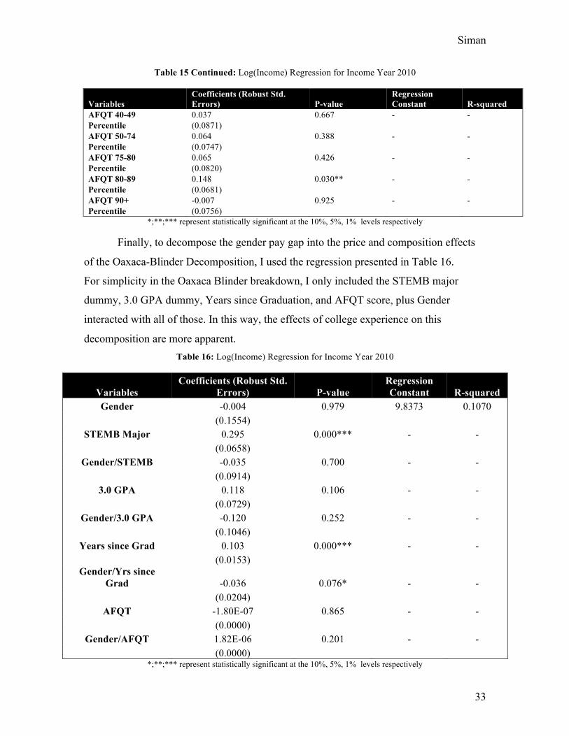
Table 15 Continued: Log(Income) Regression for Income Year 2010



AFQT 40-49 0.037 0.667 - - Percentile (0.0871)

AFQT 50-74 0.064 0.388 - - Percentile (0.0747)

AFQT 75-80 0.065 0.426 - - Percentile (0.0820)

AFQT 80-89 0.148 0.030** - - Percentile (0.0681)

AFQT 90+ -0.007 0.925 - - Percentile (0.0756)


Finally, to decompose the gender pay gap into the price and composition effects

of the Oaxaca-Blinder Decomposition, I used the regression presented in Table 16.

For simplicity in the Oaxaca Blinder breakdown, I only included the STEMB major

dummy, 3.0 GPA dummy, Years since Graduation, and AFQT score, plus Gender

interacted with all of those. In this way, the effects of college experience on this

decomposition are more apparent. Table 16: Log(Income) Regression for Income Year 2010

Variables Coefficients (Robust Std.

Errors) P-value Regression Constant R-squared

Gender -0.004 0.979 9.8373 0.1070

(0.1554)

STEMB Major 0.295 0.000*** - -

(0.0658)

Gender/STEMB -0.035 0.700 - -

(0.0914)

3.0 GPA 0.118 0.106 - -

(0.0729)

Gender/3.0 GPA -0.120 0.252 - -

(0.1046)

Years since Grad 0.103 0.000*** - -

(0.0153)

Gender/Yrs since Grad -0.036 0.076* - -

(0.0204)

AFQT -1.80E-07 0.865 - -

(0.0000)

Gender/AFQT 1.82E-06 0.201 - -

(0.0000)


Siman

34

The regression shows that a STEMB Major and Years since Graduation seem to be the

most significant factors in determining income, and thus will most likely be the main

drivers in differences in the price and composition effects. Using the methodology

outlined at the beginning of this section and the regression coefficients above, I obtained

the following results. The difference in log of income between males and female earners

in 2010 is approximately 0.231, with males having higher income, as expected. This

difference is statistically significant at the 1 percent level. The price effect is 0.176. This

indicates that if women had the same characteristics as men, the pay gap would be about

17.6 percent. The composition effect is 0.055, suggesting that if one applied the male

coefficients to female characteristics, or female “skills,” the gender gap would only be

5.5 percent. Thus, when breaking down female wages into price and composition effects

based on college experience, the larger magnitude of the price effect indicates that the

gender pay gap is mainly driven by the fact that the return of certain academic choices in

college is different for females than for males. Breaking down the price and composition

effects further, the STEMB major variable accounts for nearly all of the composition

portion of the gap. It contributes 0.062 to this effect, while AFQT adds another 0.007,

and Years since Graduation subtracts 0.014. The effect of GPA is negligible. Thus, if

females were to choose STEMB majors in the same proportion as males, the composition

effect of the decomposition would almost be entirely eliminated. This shows that the fact

that females are less likely to major in a STEMB field is the main difference that

contributes to the composition portion of the gap, which as a whole accounts for

approximately 23.8 percent of the gender pay gap. Therefore, the choice of a STEMB

major, as it is the main contributor to the composition effect, can be estimated to account

for nearly one quarter of the gender pay gap.

On the other hand, about 76.2 percent of the gender pay gap is attributed to the

price effect. In other words, this portion of the gap exists because female “skills” are

priced differently. Yet, the coefficient for choice of a STEMB major does not contribute

significantly to this gap. It only adds about 0.010 to the price effect. The main driver of

this effect is the “price” of the Years since Graduation variable, which adds 0.191 to the

price effect. The 3.0 GPA dummy also adds 0.098 to the effect (the AFQT subtracts from

the effect, getting us to the 0.176 number). In other words, the value of a STEMB major

Siman

35

is relatively equal for males and females, which is consistent with the results earlier in

this section. On the other hand, the “price” of each additional year since graduation is not

nearly as high for females as it is for males. In addition, the return of a 3.0 or better GPA

for females is also lower than it is for males, again consistent with my earlier findings.

Further investigation is needed to determine the reasons for these differences in “price”

of GPA and Years since Graduation, which is beyond the scope of this paper.

VI. Conclusion

One of the most important factors in determining future income is college

experience. By investigating the link between college major choice, GPA, and future

income, I have found that college major selection is an important component of the

gender pay gap. When controlling for ability measures and years of experience in the

working world, my results indicate that majoring in a field in Business, Economics,

Computer Science, or Engineering is a statistically significant indicator of a higher future

income, for both females and males. Women who major in these fields receive

significantly higher wages than women who do not, even if the women who majored in

the humanities had higher GPAs. The Females who choose STEMB majors do not

receive a statistically significant lower return than males. In fact, my results indicate that,

in all STEMB fields except Business and Economics, females actually may receive a

higher return from majoring in these fields than males, especially in the Computer

Science field. Thus, if more females were to choose majors in the STEMB disciplines,

perhaps we could come closer to closing the gender pay gap.

My results do not show a particularly strong link between college GPA and future

income. A cumulative GPA of 3.0 or higher suggests higher income of about 10 percent,

but the results are not statistically significant enough to conclusively confirm this fact.

Yet, the results do suggest that females do not receive as high a return in future income

from maintaining a high GPA (specifically, above a 3.0). More investigation is needed to

make a strong conclusion on this point.

Furthermore, isolating certain demographic indicators, ability measures, job

industry selection and college major choice can help to nearly fully explain the gender

pay gap. In Table 15, when controls were added for various family indicators, such as

Siman

36

marital status and birth of children, race, and also for job industry, the gender dummy

variable no longer exhibited a negative coefficient and is statistically negligible.

Lastly, breaking down the gender pay gap into the price and composition effects

of the Oaxaca-Blinder Decomposition based on various college experience indicators

reveals that about three quarters of the gap can be attributed to the price effect. That is,

most of the gender pay gap is a result of the fact that female skills are not “priced” as

high as male skills. However, a degree in a STEMB major has about the same value for

females as for males. GPA, on the other hand, is “priced” much higher for males than it is

for females. The composition effect does still account for one quarter of the gender pay

gap, and nearly all of this effect is attributed to the STEMB major characteristic. Thus, if

females and males did choose STEMB majors in the same proportion, the gender pay gap

would be significantly smaller.

Although the gender pay gap in the United States has many different causes, not

all related to undergraduate education, my study into its links to college experience has

revealed many interesting results. It is apparent that the composition of males and

females in different college majors has a significant impact on the gap. Thus, to reiterate,

if more females begin to choose STEMB majors in college, we will take large strides in

closing the gender pay gap.

Siman

37

References

Becker, Gary S., William H. J. Hubbard, and Kevin M. Murphy. 2010. Explaining the worldwide boom in higher education of women. Journal of Human Capital 4, no. 3:203-241.

Blau, Francine D. and Lawrence M. Kahn. 2000. Gender differences in pay. The Journal

of Economic Perspectives 14, no. 4:75-99. Blau, Francine D. and Lawrence M. Kahn. 2004. The US gender pay gap in the 1990s:

Slowing convergence. NBER Working Papers, no. 10853. Blau, Francine D. and Lawrence M. Kahn. 2007. The Gender Pay Gap. Economist’s

Voice 4, no. 4: Article 5. Chen, M. Keith, and Judith A. Chevalier. 2012. Are women overinvesting in education?

Evidence from the medical profession. Journal of Human Capital 6, no. 2:124-149.

Conger, Dylan, and Mark C. Long. 2010. Why are men falling behind? Explanations for

the gender gap in college. Annals of the American Academy of Political and Social Science 627, no. 1:184-214.

Covert, Bryce. 2013. We’ve moved backward in closing the gender wage gap. Forbes

Magazine. Donald, Stephen G., and Daniel S. Hamermesh. 2004. The effect of college curriculum

on earnings: Accounting for non-ignorable non-response bias. NBER Working Papers, no. 10809.

Francis, David. 2007. Why do women outnumber men in college? The NBER Digest. Gayle, George-Levi, Limor Golan, and Robert A. Miller. 2012. Gender differences in

executive compensation and job mobility. Journal of Labor Economics 30, no. 4:829-872.

Goldin, Claudia, Lawrence F. Katz, and Ilyana Kuziemko. 2006. The homecoming of

American college women: The reversal of the college gender gap. NBER Working Papers, no. 12139.

Huffman, Matt L. and Philip N. Cohen. 2004. Racial wage inequality: Job segregation

and devaluation across U.S. labor markets. American Journal of Sociology 109, no. 4:902-936.

Izzo, Phil. 2012. Which college majors pay best? The Wall Street Journal.

Siman

38

Johnson, William G. and James Lambrinos. 1985. Wage discrimination against handicapped men and women. Journal of Human Resources 20, no. 2:264-277.

Lin, Eric S. 2010. Gender wage gaps by college major in Taiwan: Empirical evidence

from the 1997-2003 Manpower Utilization Survey. Economics of Education Review 29, no. 1:156-164.

National Longitudinal Survey of Youth 1997 (1997-2011). Bureau of Labor Statistics.

Retrieved from http://www.bls.gov/nls/nlsy97.htm. Neumark, David. 1988. Employers’ Discriminatory Behavior and the Estimation of Wage

Discrimination. Journal of Human Resources 23, no. 3:279-295. U. S. Bureau of Labor Statistics. 2011. Highlights of Women’s Earnings in 2010. Report

1031. U. S. Department of Education. 2012. Fast Facts: Degrees Conferred by Sex and Race.

The Condition of Education 2012. Waldfogel, Jane. 1998. Understanding the “Family Gap” in Pay for Women with

Children. Journal of Economic Perspectives 12, no. 1:137-156. Weinberger, Catherine. 1998. Race and Gender Wage Gaps in the Market for Recent

College Graduates. Industrial Relations 37, no. 1: 67-84. Wiswall, Matthew, and Basit Zafar. 2011. Determinants of college major choice:

Identification using an information experiment. Federal Reserve Bank of New York Staff Reports, no. 500.

Zafar, Basit. 2013. College major choice and the gender gap. Journal of Human

Resources 48, no. 3:545-595.

undergraduate education and the gender wage gap: an ... · pdf fileduke university durham, ......

Documents