uncertainty, timevarying fear, and asset prices
TRANSCRIPT

THE JOURNAL OF FINANCE • VOL. LXVIII, NO. 5 • OCTOBER 2013
Uncertainty, Time-Varying Fear, and Asset Prices
ITAMAR DRECHSLER∗
ABSTRACT
I construct an equilibrium model that captures salient properties of index optionprices, equity returns, variance, and the risk-free rate. A representative investormakes consumption and portfolio choice decisions that are robust to his uncertaintyabout the true economic model. He pays a large premium for index options becausethey hedge important model misspecification concerns, particularly concerning jumpshocks to cash flow growth and volatility. A calibration shows that empirically con-sistent fundamentals and reasonable model uncertainty explain option prices andthe variance premium. Time variation in uncertainty generates variance premiumfluctuations, helping explain their power to predict stock returns.
KNIGHTIAN UNCERTAINTY—AMBIGUITY ABOUT the true model governingfundamentals—can be an important factor influencing investors’ consumptionand portfolio choice decisions. Incorporating it into asset pricing models cantherefore shed light on sources of asset return premiums and time variation inprices. In this paper, I construct an equilibrium model with a representativeinvestor who has model uncertainty that varies in intensity over time.1 A cali-bration of this model is shown to capture a broad set of features of equity andequity index option prices. In particular, the model generates two prominentfeatures of index options that represent a challenge to equilibrium models:(i) the large premium embedded in their prices, called the variance premium,and (ii) the shape of their implied volatility surface, especially the “volatilityskew.” This is the name given to the pattern in the implied volatilities of short-maturity puts, which are high for out-of-the-money (otm) puts and decreasesharply as put moneyness increases. At the same time, the model matchesthe salient properties of equity returns and the risk-free rate, the dynamics of
∗Itamar Drechsler is at Stern School of Business, New York University. I my grateful to mycommittee, Amir Yaron (Chair), Rob Stambaugh, and Stavros Panageas. I also thank Andy Abel,Ravi Bansal (discussant), Joao Gomes, Lars Hansen, Philipp Illeditsch, Jakub Jurek, RichardKihlstrom, Feifei Li (discussant), Jun Liu, Nick Roussanov, Freda Song, Nick Souleles, LukeTaylor, Jessica Wachter, Paul Zurek, and seminar participants at Wharton, Chicago Booth Schoolof Business, Columbia GSB, Princeton, NYU Stern, the University of Rochester, the 2009 WesternFinance Association meeting (San Diego), the 2009 Stanford Institute for Theoretical Economics(SITE) workshop, and the 2010 American Finance Association meeting (Atlanta) for helpful com-ments. I thank Nim Drechsler and contacts at Citigroup and CSFB for options data. I am alsoindebted to the Editor, Cam Harvey, and to an anonymous referee for numerous comments thatsignificantly improved the paper.
1 I use the terms Knightian uncertainty, model uncertainty, and ambiguity interchangeably.
DOI: 10.1111/jofi.12068
1843

1844 The Journal of Finance R©
conditional equity variance, and the moments of cash flows (consumption anddividends). The model is the first, to my knowledge, to successfully capture thisbroad set of features. It does this with a modest risk aversion of five, and as Iexplain below, a quantitatively reasonable level of model uncertainty.
Prior studies find that equity index option prices incorporate a considerablepremium.2 A good measure of this is the difference between option-impliedexpectations of return variance (which correspond to the VIX) and statistical(i.e., true) expectations of return variance (see Section II for details). The option-implied expectation is equivalent to the price of a variance swap, a contract thatpays the buyer the realized variance over the term of the contract. Buying theswap provides the buyer with protection against high realized variance. Thus,the difference between the swap price and the true expectation of variance isthe (variance) premium investors pay for this hedge. As I document below, atthe one-month horizon the variance premium is large. Furthermore, its timeseries has predictive power for stock returns over horizons of a few months. Asecond prominent feature of index option prices is the shape of their impliedvolatility surface. Going back to at least Rubinstein (1994), academic studieshave been concerned with understanding the sources of the volatility skew,which implies that otm put options are expensive relative to the benchmarkBlack–Scholes–Merton model (see, for example, Bates (2003)).
In this paper, I show that a desire by the representative investor to hedgehis model uncertainty concerns naturally leads to a price premium in indexoptions, and that the magnitude of the premium is sensitive to his level ofmodel uncertainty. In the model, the representative investor has in mind abenchmark/reference model that represents his best estimate of the dynamicsof economic fundamentals. However, due to model uncertainty, he is worriedthat this reference model is incorrect in some ways. Moreover, he wants hisconsumption and portfolio choice decisions to be robust to this possibility. Hetherefore considers the possibility that the true model actually lies in a set ofalternative models.3 To ensure that his model uncertainty concerns are rea-sonable, he considers alternative models that are statistically difficult to dif-ferentiate from the reference model and hence difficult to reject empirically.To make decisions that are robust across the set of alternative models, theinvestor optimally evaluates his decisions under whichever alternative modelrepresents the “worst case.” This worst-case alternative model is determinedby perturbing (i.e., changing) the reference model in whichever ways are mostdamaging to the investor’s utility, while remaining difficult to rule out based onhistorical data. The worst-case perturbations represent the potential modelingerrors that most worry the investor.
2 See, for example, Coval and Shumway (2001), Pan (2002), Bakshi and Kapadia (2003), Eraker(2004), and Carr and Wu (2009). Singleton (2006) contains a review of option pricing studies.
3 My framework builds on the literature on robust control, pioneered by Hansen and Sargent.See, for example, Anderson, Hansen, and Sargent (2003), Hansen et al. (2006), and Hansen andSargent (2008). The preferences are in the class of recursive multiple priors utility of Epstein andSchneider (2003).

Uncertainty, Time-Varying Fear, and Asset Prices 1845
Since the investor evaluates his decisions under the worst-case model, hisconcerns about model errors have an important impact on asset prices. Forexample, one of the investor’s concerns is that his reference model overstatesthe mean of the persistent component in cash flow growth rates. Consequently,he decreases the price he is willing to pay for equity, which increases the ex-pected equity return. In the calibrated model, the investor optimally allocatesthe biggest fraction of his uncertainty to concerns about the reference model’sspecification of jump shocks. Jump shocks are infrequent but relatively largeshocks to the expected growth and growth volatility processes. The investoris concerned that the reference model underestimates their frequency or mag-nitude, which means they are amplified under the worst-case model. This in-creases the price the investor is willing to pay for variance swaps and helpsgenerate a large variance premium and steep implied volatility skew. Statedanother way, the investor knows that, if these model uncertainty concerns ma-terialize, the resulting realized variance will be high. As index options willhave a high payoff if this occurs, they provide a hedge to these model uncer-tainty concerns and the investor is therefore willing to pay a large premium forthem. A further implication is that the size of the variance premium will varyto reflect fluctuations in the investor’s level of uncertainty. This, in turn, willendow it with power to predict equity returns.
The framework constructed in this paper involves model uncertainty over aricher set of economic dynamics than have been possible in previous applica-tions of robust control or ambiguity aversion. Specifically, the calibrated modelincorporates uncertainty over a reference model whose dynamics include (i)a persistent component in expected cash flow growth, (ii) stochastic volatility,and (iii) jumps in the expected growth and growth volatility processes.4 Thisrich set of dynamics is required for the model to be flexible enough to confronta large set of features of equity and options prices, and to allow model un-certainty to operate through multiple channels. The framework also extendsprevious models in allowing for time-variation in the representative investor’slevel of model uncertainty and by separating risk aversion and intertemporalelasticity of substitution (IES). Both of these features are important for thecalibrated model to match the data. Despite this increased complexity, I pro-vide analytical expressions for equity prices and the variance premium, whichshow the impact of uncertainty concerns on these quantities. Having analyticalexpressions also allows for precise calculation of option prices and the impliedvolatility surface.
The calibration of the model matches a broad set of features of cash flowsand asset prices. These include “traditional” targets of equilibrium asset pric-ing models—the high equity premium, low risk-free rate, and excess volatil-ity of equity returns relative to fundamentals. At the same time, the model
4 Tractability is an issue when solving for equilibrium prices in models with uncertainty. Manyfinancial applications focus on either log utility, which aids tractability, or i.i.d or single statevariable environments. Some examples are Kleshchelski and Vincent (2007), Ulrich (2013), Brevik(2008), Trojani and Sbuelz (2008), Maenhout (2004), and Uppal and Wang (2003).

1846 The Journal of Finance R©
generates the aforementioned features of index option prices, which are notcaptured by leading equilibrium asset pricing models.5 The calibrated modelgenerates a variance premium that is large and positive, as in the data, and haspredictive power for one- and three-month excess stock returns that is empir-ically consistent. Furthermore, the calibration matches the implied volatilitysurface, with an implied volatility skew that is very steep for one-month optionsand decays steadily as the horizon increases. Finally, the model also matchesthe dynamic properties of conditional equity variance, such as its persistenceand volatility, and the higher moments of equity returns.
The calibration achieves its fit to the data using a level of model uncertaintyunder which the worst-case model is difficult to reject empirically; roughlyspeaking, it implies that one cannot reject at the 10% level the null hypothesisthat the worst-case model generates the data. It is therefore reasonable forthe investor to be concerned about this model. At the same time, the levelof relative risk aversion used in the model is only five, which is much belowthe risk aversion levels used in most macro-finance asset pricing models.6 If,however, uncertainty is turned off, then a much higher risk aversion of 13 isrequired to match the equity premium under the calibration, yet the variancepremium generated in that case is too small.
The paper is organized as follows. Section I relates the paper to the litera-ture. Section II discusses the data and empirical evidence. Section III presentsthe model. Section IV solves for the representative agent’s equilibrium valuefunction and worst-case model. Section V solves for equilibrium asset prices.Section VI calibrates the model and assesses its fit to the data. Section VII con-cludes. The Appendix contains technical material, while the Internet Appendixcontains additional analysis and remaining technical details.7
I. Research Setting
This paper is part of a new literature that bridges the gap between re-search on equilibrium models of asset prices and studies of reduced-form op-tion pricing models. The findings of the reduced-form studies are informativefor equilibrium models, whose traditional set of targets—the equity premiumand risk-free rate—are too limited to provide a full picture of the sources ofrisk and uncertainty impacting prices. In particular, a number of studies (e.g.,Pan (2002), Eraker (2004), and Broadie, Chernov, and Johannes (2007)) find
5 Du (2010) shows that the habit models of Campbell and Cochrane (1999) and Menzly, Santos,and Veronesi (2004) are inconsistent with the implied volatility skew of index options, while Backus,Chernov, and Martin (2011) and Du (2010) show that this is also the case for the rare disastersmodel of Barrow (2006). Below I document that the long-run risk models of Bansal and Yaron(2004) and Bansal, Kiku, and Yaron (2007) produce a variance premium that is much too smallrelative to the data.
6 Barillas, Hansen, and Sargent (2009) highlight the result that, with model uncertainty, adesire for robustness allows for a reduction in the risk aversion coefficient.
7 The Internet Appendix may be found in the online version of this article.

Uncertainty, Time-Varying Fear, and Asset Prices 1847
that jumps are important for describing the time series of equity returns andvolatility, and that jump risk is significantly priced in options. The equilibriummodel in this paper incorporates these features and is consistent with thesefindings. Recent studies also focus on the variance premium as an importantobject of interest, as it is in this paper. Broadie, Chernov, and Johannes (2009)argue that looking at the wedge between implied and realized volatility (es-sentially the variance premium) is the most informative way to analyze thepremium in option prices. Todorov (2010) emphasizes the importance of jumpsin explaining the dynamics and pricing of the variance premium, while Boller-slev, Gibson, and Zhou (2011) and Bollerslev, Tauchen, and Zhou (2009) findthat their variance premium measures have significant predictive power forstock returns at horizons of a few months.
There are a few examples of equilibrium models that do target features of op-tion prices. These include Benzoni, Collin-Dufresne, and Goldstein (2011), Du(2010), Eraker and Shaliastovich (2008), Liu, Pan, and Wang (2005; hereafterLPW), and Shaliastovich (2011). LPW is discussed below, while a discussion ofthese other papers and additional potential approaches is left to the InternetAppendix. None of these other models, however, considers the full set of equity,option, and variance features addressed by this paper, and in particular, noneanalyzes the variance premium.
LPW are the first to use model uncertainty to explain option prices in equi-librium. In their model, investors’ uncertainty about rare events explains theskew in index option implied volatilities. In contrast to this paper, the model inLPW has i.i.d. dynamics and equates the volatility of consumption and returns.As a result, it cannot capture the “excess volatility” of returns, the dynamics ofconditional variance, or return predictability by the variance premium. LPW’scalibration is limited to the equity premium and volatility skew. They do notconsider the variance premium or other moments of equity returns, the risk-free rate, or cash flows. In addition, jumps in LPW represent “rare disasters,”that is, rare and very large jumps in the aggregate endowment, while in thispaper jumps occur on average every one to two years and are moderate by com-parison. In LPW, jumps enter into the level of cash flows, while the jumps hereare in the expected growth rate of cash flows, so the level of cash flows evolvessmoothly.8 Finally, LPW do not quantify the amount of uncertainty impliedby their calibration, while this quantity is an important part of this paper’scalibration.
This paper is also related to Anderson, Ghysels, and Juergens (2009), whoconstruct measures of the economy-wide level of (Knightian) uncertainty usingsurvey forecasts and find that these measures predict stock returns in both thetime series and the cross section. This paper also creates a proxy for economy-wide model uncertainty based on survey forecasts and shows that it closelytracks fluctuations in the variance premium.
8 Benzoni, Collin-Dufresne, and Goldstein (2011) is the first paper to model jumps in the expectedgrowth process.

1848 The Journal of Finance R©
Methodologically, this paper contributes to the literature applying modeluncertainty to financial applications. Maenhout (2004) solves for the equitypremium in an economy with a robust investor that has recursive utility. Heexogenously modifies the canonical robust control model to induce wealth inde-pendence and analytical tractability. This exogenous modification is also usedin Uppal and Wang (2003) and LPW. In contrast, wealth-independence arisesendogenously in the framework of this paper.
This paper is also related to Drechsler and Yaron (2011), who build an ex-tended long-run risks (Bansal and Yaron (2004)) model with jump shocks thatcaptures the size and predictive power of the variance premium. They do notconsider model uncertainty, a central driver of asset prices in this paper, anddo not examine the option-implied volatility surface or the connection betweenoption prices and measures of model uncertainty. While in this paper time-variation in the perceived risk of jumps also drives fluctuations in the variancepremium, it now arises from the combination of reference-model jump risks andfluctuations in model uncertainty fears. Moreover, since model uncertainty en-dogenously amplifies concerns about jump shocks, less is needed in terms ofphysical jumps, and the model is able to capture the equity premium and op-tion prices with a significantly lower risk aversion of five. Finally, the model inthis paper generates stochastic return volatility from two channels, stochasticcash flow volatility and stochastic uncertainty. This makes the variance pre-mium imperfectly correlated with conditional volatility and a better predictorof equity returns than overall variance.
Finally, a number of papers prominently feature uncertainty in an assetpricing context, though under the Bayesian approach. Pastor (2000), Pastorand Stambaugh (2000), and Avramov (2004) use a Bayesian approach to assetallocation. Avramov (2002) and Pastor and Stambaugh (2011) assess returnpredictability, Brennan and Xia (2001) model how learning about predictabil-ity impacts asset allocation, and Veronesi (2000) shows that Bayesian filteringon the part of investors can induce interesting dynamics in asset prices. Thesepapers analyze different problems from the one studied here, and none of themconstructs an equilibrium model of prices based on preferences and fundamen-tals, assuming instead an exogenous process for returns and/or the pricingkernel.
II. Data
The variance (risk) premium is defined as the difference between the riskneutral and physical (i.e., true/statistical) expectations of total stock marketreturn variance for a given horizon. I focus on a one-month variance pre-mium. Hence, the one-month variance premium at time t, denoted vpt, equalsEQ
t [∫ t+1
t (d ln Rm,s)2] – Et[∫ t+1
t (d ln Rm,s)2], where ln Rm,s is the (log) return on themarket and Q denotes the risk-neutral probability measure.
Demeterfi et al. (1999) and Britten-Jones and Neuberger (2000) show that,when the underlying asset price is continuous, the risk-neutral expectation of

Uncertainty, Time-Varying Fear, and Asset Prices 1849
variance for an asset is given by the value of a portfolio of European calls on thatasset. This follows by demonstrating a trading strategy that uses a portfolio ofoptions to replicate a variance swap on the asset. In other words, the strategy’spayoff is the asset’s realized variance. The risk-neutral expectation of thispayoff then follows from the cost of the strategy, which is the cost of the optionportfolio. Jiang and Tian (2005) and Carr and Wu (2009) extend this result tothe case in which the asset follows a jump-diffusion. Note that this approachis “model-free” since it does not depend on any particular option pricing model.The Chicago Board Options Exchange (CBOE) uses this model-free methodto calculate the VIX index as the risk-neutral expectation of variance for theS&P 500 over the subsequent 30 days. I obtain closing values of the VIX fromthe CBOE and use it as my measure of risk-neutral expected variance. Moreprecisely, since the VIX index is reported in annualized “vol” terms, I square itto put it in “variance” space and divide by 12 to get a monthly quantity. I referto the resulting series as squared VIX. For each month, I use the value of theVIX on the last day.
To measure vpt one also needs a conditional forecast of total return variationunder the physical measure. Measures of the realized variance of the marketfor a given month can be obtained by summing up the squared five-minutelog returns on the S&P 500 futures and on the S&P 500 index over the wholemonth.9 I obtain the high frequency data used to construct these realized vari-ance measures from TICKDATA. To get a conditional forecast series, I use theone-step-ahead forecasts from a simple time-series model. I project the futuresrealized variance on the value of the squared VIX at the end of the previousmonth and on a lagged realized variance measure. The one-step-ahead forecastseries from this regression serves as the proxy for the conditional expectationof total return variance under the physical measure. The difference betweenthe risk neutral expectation, given by the squared VIX, and the contemporane-ous conditional forecast gives the time series of one-month variance premiumestimates. The intuition that the variance premium is a premium paid for in-surance (against high realized variance) implies that it should be nonnegativemonth-by-month. That is, the physical expectation of variance should be lessthan the risk-neutral one. For 239 out of 240 months, this is not a problem sincein 238 months the variance premium estimate is positive, while one month hasa tiny negative value and can be considered zero. I impose the theoretical re-striction on the remaining month by truncating the variance forecast proxyat the value of the squared VIX, implicitly truncating the variance premiumestimate to zero. The impact of this truncation on the results, which is small,
9 Estimating realized variance for highly liquid assets via the summation of high-frequencysquared returns has become the standard method in practical applications (see, for example,Andersen et al. (2001), Andersen, Bollerslev, and Diebold (2007), and Bollerslev, Gibson, andZhou (2011)). A five-minute sampling frequency provides a good balance between the improvedestimation precision afforded by a finer sampling of the data and the greater measurement noiseintroduced into such increasingly finer sampling due to bid-ask spreads, price discreteness, andother microstructure issues (see, for example, Hansen and Lunde (2006)).
1850 The Journal of Finance R©
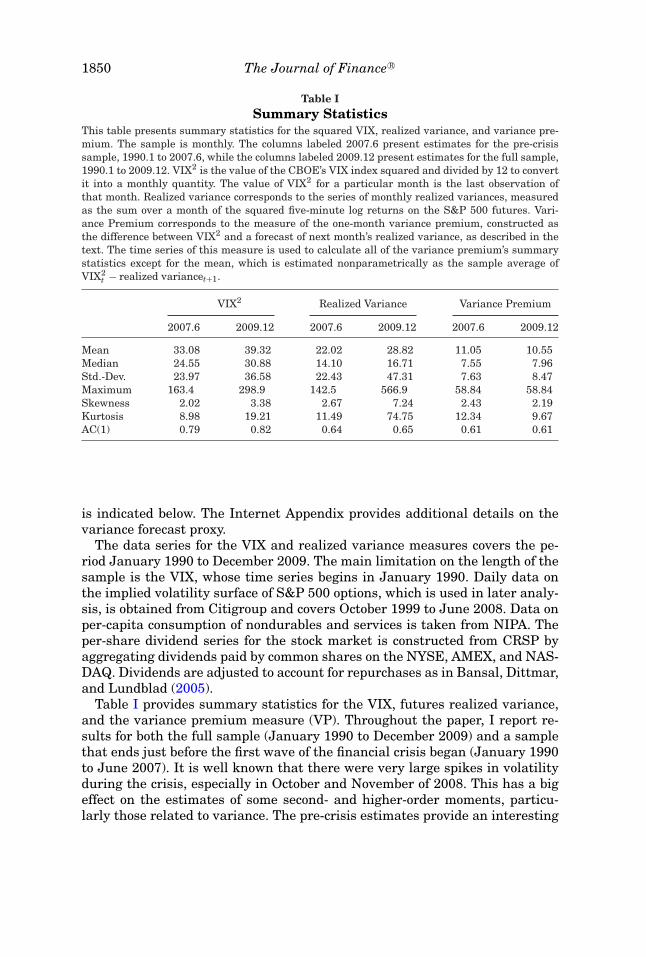
Table ISummary Statistics
This table presents summary statistics for the squared VIX, realized variance, and variance pre-mium. The sample is monthly. The columns labeled 2007.6 present estimates for the pre-crisissample, 1990.1 to 2007.6, while the columns labeled 2009.12 present estimates for the full sample,1990.1 to 2009.12. VIX2 is the value of the CBOE’s VIX index squared and divided by 12 to convertit into a monthly quantity. The value of VIX2 for a particular month is the last observation ofthat month. Realized variance corresponds to the series of monthly realized variances, measuredas the sum over a month of the squared five-minute log returns on the S&P 500 futures. Vari-ance Premium corresponds to the measure of the one-month variance premium, constructed asthe difference between VIX2 and a forecast of next month’s realized variance, as described in thetext. The time series of this measure is used to calculate all of the variance premium’s summarystatistics except for the mean, which is estimated nonparametrically as the sample average ofVIX2
t − realized variancet+1.
VIX2 Realized Variance Variance Premium
2007.6 2009.12 2007.6 2009.12 2007.6 2009.12
Mean 33.08 39.32 22.02 28.82 11.05 10.55Median 24.55 30.88 14.10 16.71 7.55 7.96Std.-Dev. 23.97 36.58 22.43 47.31 7.63 8.47Maximum 163.4 298.9 142.5 566.9 58.84 58.84Skewness 2.02 3.38 2.67 7.24 2.43 2.19Kurtosis 8.98 19.21 11.49 74.75 12.34 9.67AC(1) 0.79 0.82 0.64 0.65 0.61 0.61
is indicated below. The Internet Appendix provides additional details on thevariance forecast proxy.
The data series for the VIX and realized variance measures covers the pe-riod January 1990 to December 2009. The main limitation on the length of thesample is the VIX, whose time series begins in January 1990. Daily data onthe implied volatility surface of S&P 500 options, which is used in later analy-sis, is obtained from Citigroup and covers October 1999 to June 2008. Data onper-capita consumption of nondurables and services is taken from NIPA. Theper-share dividend series for the stock market is constructed from CRSP byaggregating dividends paid by common shares on the NYSE, AMEX, and NAS-DAQ. Dividends are adjusted to account for repurchases as in Bansal, Dittmar,and Lundblad (2005).
Table I provides summary statistics for the VIX, futures realized variance,and the variance premium measure (VP). Throughout the paper, I report re-sults for both the full sample (January 1990 to December 2009) and a samplethat ends just before the first wave of the financial crisis began (January 1990to June 2007). It is well known that there were very large spikes in volatilityduring the crisis, especially in October and November of 2008. This has a bigeffect on the estimates of some second- and higher-order moments, particu-larly those related to variance. The pre-crisis estimates provide an interesting

Uncertainty, Time-Varying Fear, and Asset Prices 1851
comparison across samples and allow one to assess the data when the influenceof the outlier months is excluded.10
The table shows that the mean of the variance premium is sizable in compar-ison with those of the squared VIX and realized variance. Between a quarterand a third of the risk-neutral expectation of variance is a premium. More pre-cisely, it represents an insurance premium, since the price of the variance swapis greater than its average payoff. As the table shows, the variance premium isalso quite volatile. Note further that all three variance-related series displaysignificant deviations from normality. The mean to median ratio is large, theskewness is positive and greater than zero, and the kurtosis is clearly muchlarger than three. Across the two samples the variance premium statistics aresimilar, though in the full sample the mean is a bit lower, the standard devia-tion a bit higher, and the kurtosis a bit lower but still very high.11 There arebigger changes across the samples in the statistics of the other two series. Inparticular, the standard deviations and higher moments all increase dramati-cally, due to the tremendous spike in volatility in the fall of 2008 and the firstquarter of 2009.12
Table II shows return predictability regressions. There are two sets ofcolumns with regression estimates. The first set shows OLS estimates andthe second provides estimates from robust regressions, which downweight theinfluence of outliers on the estimates, providing a check that they do not drivethe results. The robust regression R2s reported are calculated as the ratio ofthe variance of the regression forecast to the variance of the dependent vari-able, which corresponds to the usual R2 calculation in the case of OLS. Thefirst two regressions are one-month-ahead forecasts using the variance pre-mium as a univariate regressor, while the third forecasts one quarter ahead.The quarterly return series is overlapping. The last two specifications add theprice–earnings ratio, a commonly used variable for predicting returns. As aunivariate regressor, the variance premium can account for about 1.5% to 4.9%of the monthly excess return variation. The multivariate regressions lead to afurther increase in the R2. In conjunction with the price–earnings ratio, thein-sample R2 can increase to over 10%. Note that in all cases the variancepremium enters with a significant positive coefficient, which will be shown to
10 The starting point of the crisis is often marked by the June 2007 collapse of two Bear Stearnshedge funds and the August 2007 “quant crisis.” However, the results are similar if the pre-crisissample is extended until August 2008.
11 The truncation of the negative VP month only has a noticeable impact on the kurtosis andskewness of the full-sample VP. Without truncation, the kurtosis of VP rises to 10 and the skewnessis 1.60.
12 I also estimate moments for VP for the sample 1986 to 2009 and find that they are broadlysimilar to those for the post-1990 sample, with an estimated mean and standard deviation of thevariance premium of 9.44 and 12.77, respectively. I obtain a proxy for VIX for the pre-1990 sampleby using VXO (the “old” VIX), which is available from 1986. I regress VIX on VXO and a constantwithin the 1990 to 2009 sample and use the estimated relationship to obtain fitted values forVIX for the pre-1990 sample. For October 1987, I also replace the high-frequency futures realizedvariance with daily realized variance because of the well-documented breakdown in futures tradingthat occurred during the stock market crash.

1852 The Journal of Finance R©
Table IIReturn Predictability by the Variance Premium
This table presents return predictability regressions. The sample is monthly. The top panel presentsthe estimates for the pre-crisis sample, 1990.1 to 2007.6, while the bottom panel shows the esti-mates for the full sample, 1990.1 to 2009.12. Reported t-statistics for OLS are Newey–West (HAC)corrected. VP is the variance premium. P/E is the price–earnings ratio for the S&P 500. The de-pendent variable is the log excess return (annualized and in percent) on the S&P 500 index overthe following one and three months, as indicated. The three-month returns series is overlapping.Robust Reg. denotes estimates from robust regressions using a bisquare weighting function. Thereported robust regression pseudo-R2s are calculated as the ratio of the variance of the regressionforecast to the variance of the dependent variable, which corresponds to the usual R2 calculationin the case of OLS.
Regressors OLS Robust Reg.
X1 X2 β1 β2 R2(%) β1 β2 R2(%)
Pre-Crisis Sample (1990.1 to 2007.6)
rt+1 V Pt 0.74 1.44 1.08 3.05(t-stat) (2.18) (2.71)
rt+1 V Pt−1 1.32 4.48 1.22 3.88(t-stat) (3.96) (3.04)
rt+3 V Pt 0.87 6.15 0.88 6.29(t-stat) (3.53) (4.26)
rt+1 V Pt log (P/E)t 1.31 −47.43 8.08 1.69 −48.85 10.22(t-stat) (2.89) (−3.07) (4.14) (−4.28)
rt+1 V Pt−1 log (P/E)t 2.06 −56.67 13.64 1.95 −56.34 12.82(t-stat) (4.73) (−3.51) (4.71) (−4.86)
Full Sample (1990.1 to 2009.12)
rt+1 V Pt 0.80 1.72 1.40 5.24(t-stat) (2.25) (3.99)
rt+1 V Pt−1 1.38 5.10 1.46 5.68(t-stat) (3.97) (4.11)
rt+3 V Pt 0.99 6.93 1.11 8.62(t-stat) (3.98) (5.72)
rt+1 V Pt log (P/E)t 1.37 −25.03 4.69 1.86 −23.74 7.30(t-stat) (3.70) (−1.49) (4.67) (−2.86)
rt+1 V Pt−1 log (P/E)t 2.17 −33.65 10.34 2.06 −30.79 9.20(t-stat) (5.32) (−2.20) (5.09) (−3.63)
be consistent with the theory in this paper. In addition, the robust regressionestimates agree in both magnitude and sign with the OLS estimates. Compar-ing across the two samples, the coefficient estimates and predictive R2s do notchange greatly.13
13 If the VP series is not truncated at zero (which affects only the full sample) then the predictivepower is actually a bit greater. I also split the full sample into equal-length subperiods, January1990 to December 1999, and January 2000 to December 2009, and estimate the predictability re-gressions within the subsamples. The OLS estimates for the coefficient on the variance premium in

Uncertainty, Time-Varying Fear, and Asset Prices 1853
Table IIIReturn Predictability by the Variance Premium: Rolling RegressionsThis table presents return predictability regressions based on a VP series constructed from varianceforecasts taken from rolling regressions. The sample is monthly. The columns labeled 2007.6present estimates for the pre-crisis sample 1990.1 to 2007, while the columns labeled 2009.12 arefor the full sample, 1990.1 to 2009.12. The first 24 data points (months) are used to initialize therolling regression for the variance forecast, so the effective sample for return prediction begins in1992.1. Reported t-statistics are Newey–West (HAC) corrected. P/E is the price–earnings ratio forthe S&P 500. The dependent variable is the log excess return (annualized and in percent) on theS&P 500 index over the following one and three months, as indicated. The three-month returnsseries is overlapping.
Regressors OLS (2007.6) OLS (2009.12)
X1 X2 β1 β2 R2(%) β1 β2 R2(%)
rt+1 V Pt 0.71 2.21 0.73 1.86(t-stat) (2.94) (2.39)
rt+1 V Pt−1 1.00 4.35 1.28 5.69(t-stat) (3.85) (4.16)
rt+3 V Pt 0.70 6.79 0.92 7.63(t-stat) (3.38) (3.98)
rt+1 V Pt log (P/E)t 1.43 −60.91 12.61 1.08 −21.21 4.29(t-stat) (5.84) (−4.77) (3.98) (−1.27)
rt+1 V Pt−1 log (P/E)t 1.91 −70.94 17.86 1.79 −29.00 10.10(t-stat) (4.79) (−4.89) (4.45) (−1.69)
As an additional robustness check, I construct the VP series using one-step-ahead variance forecasts from regressions estimated on a rolling basis usingonly past data, rather than the whole sample. The first 24 months are used toinitialize the rolling regression estimates, so this VP series begins in January1992. Table III repeats the return predictability regressions using this VP se-ries. A comparison with Table II shows that the results are largely unchanged.
A. An Empirical Proxy for the Level of Model Uncertainty
Figure 1 graphs an empirical proxy for the economy-wide level of model un-certainty. I measure the level of model uncertainty by the dispersion in theset of forecasts of next quarter’s real GDP growth, from the Philadelphia Fed’sSurvey of Professional Forecasters (SPF). The dispersion is calculated simplyas the standard deviation in the growth forecasts, which are reported near thebeginning of every quarter. I take the dispersion as a proxy for the size of thealternative set of reasonable models that the representative investor considersat each point in time. This measure maps nicely to the way time-varying un-certainty is formally modeled below. Moreover, information asymmetry shouldnot be an important issue for forecasting an aggregate quantity such as GDP,since the relevant information is widely reported and discussed in the public
the one-month-ahead regressions are 1.07 for the earlier subperiod and 0.75 for the later subperiod.The difference of 0.32 is not statistically significant, with a t-statistic of 0.49.

1854 The Journal of Finance R©
1
2
3
4
5
6
7
.004
.006
.008
.010
.012
.014
.016
19911990 1992 1993 1994 1995 1996 1997 1998 1999 2000 2001 2002 2003 2004 2005 2006 2007 2008 2009
VP^0.5Forecast Dispersion
vp^0
.5D
ispersion
Figure 1. Forecast dispersion and variance premium. The figure plots the standard devia-tion in forecasts of next quarter’s real GDP growth from the Survey of Professional Forecasters(SPF) versus the square root of VP at the end of the previous quarter. The sample is 1990Q1 to2009Q4. The correlation of the two series is 0.54 with a robust standard error of 0.14.
domain. It is therefore natural to interpret different forecasts as the productof different economic models. The forecast dispersion captures the size of thecross section of model forecasts that the representative investor considers (i.e.,the alternative set).
The figure plots the quarterly dispersion measure along with the squareroot of VP at the end of the previous quarter. Taking the square root putsboth measures in standard deviation terms. The comovement between the twoseries is striking. Their correlation is 0.54, with a standard error of 0.14. Thetwo series tend to spike around the same time, particularly in 1990 to 91,1994, 2001 to 2002, and the recent crisis. Note that the dispersion measurebegins to rise from a low level in the third quarter of 2007, when the first signsof the economic crisis emerge. One exception to their strong comovement isthe financial crisis of 1998, which caused a sharp spike in the options marketwithout a corresponding strong increase in forecast dispersion. Perhaps thisis due to the short-lived nature of this episode, which appeared to be largelyinternational in nature and not directly related to domestic economic events.Overall, the figure provides support for a link between time-variation in modeluncertainty and the premium in index option prices, a relationship predictedby the model developed below.14
III. Model Framework
The setting for the model is an infinite-horizon, continuous-time exchangeeconomy with a representative investor who has utility over consumptionstreams. This investor has in mind a benchmark or reference model of
14 Ben-David, Graham, and Harvey (2010) ask CFOs for the 10th and 90th percentiles of theirpredictive distribution for next year’s S&P 500 return. The average 10th percentiles series, whichis informative about CFOs’ concerns of reasonable worst-case return outcomes, has a correlationof −0.63 and −0.76 with the dispersion series and its one-period lead, respectively, over the sampleperiod 2000Q2 to 2010Q1. The relationship between these two series, which are drawn fromdifferent sources, is evidence that the uncertainty fluctuations measured by the dispersion seriesare not idiosyncratic to professional forecasters, but reflect economy-wide variation.

Uncertainty, Time-Varying Fear, and Asset Prices 1855
the economy that represents his best estimate of the economy’s dynamics.However, the investor does not fully trust that his model is correct, causinghim to worry that the true model lies in a set of alternative models that aredifficult for him to reject empirically. These alternative models are “close” tothe reference model because they are difficult to distinguish from it statisti-cally. The investor guards against model uncertainty by making consumptionand portfolio choice decisions that are robust across the set of alternative mod-els. This is equivalent to evaluating future prospects under whichever is theworst-case model in the alternative set. I now formalize this setup in detail.
A. The Reference Model
Let Yt ∈ Rn denote the vector of state variables. It follows a continuous-time
affine jump-diffusion:15
dYt = μ(Yt)dt + �(Yt)dZt + ξt · dNt, (1)
where Zt is a Brownian motion in Rn, �(Yt) is a matrix, and μ(Yt), ξt, and
Nt are vectors. The term ξt · dNt denotes component-wise multiplication of thejump sizes in the random vector ξt and the increments in the vector of Poisson(counting) processes Nt. The Poisson arrivals are conditionally independentand arrive with a time-varying intensity given by the vector lt ∈ R
n. The jumpsizes in ξt are assumed to be i.i.d. Let ψ(u) denote the vector that stacks themoment-generating functions of the jump sizes; its kth component is ψk(uk) =E[exp(ukξk)], which completely characterizes the distribution of the jump sizeξk. For convenience, let log consumption and dividends, ln Ct and ln Dt, be inYt, and let δc and δd be vectors that select them from Yt, that is, ln Ct = δ′
cYtand ln Dt = δ′
dYt. Although ln Ct is in Yt, I maintain the standard assumptionthat the dynamics of Yt do not depend on ln Ct, so that equilibrium quantitiesare homogeneous in the level of consumption.
The drift, diffusion, and jump intensity functions have an affine structure.The drift is given by
μ(Yt) = μ + KYt,
where μ ∈ Rn and K ∈ R
n×n. The diffusion covariance matrix �(Yt)�(Yt)′ isassumed to have a block-diagonal structure, where each block is affine. Thisstructure is necessitated by the model uncertainty setup, as explained below.Towards that end, let Yt = (Y ′
1,t, Y ′2,t)
′ be a partition of the state vector. Thispartition determines which subset of the dYt dynamics the investor is uncertainabout. The diffusion covariance matrix takes the block-diagonal form
�(Yt)�(Yt)′ =[
�1,t�′1,t 0
0 �2,t�′2,t
],
15 The notation used here for the jump-diffusion specification is similar to that in Duffie, Pan,and Singleton (2000) and Eraker and Shaliastovich (2008).

1856 The Journal of Finance R©
where the upper block corresponds to Y1,t and the lower block to Y2,t. Thequantity �1,t�
′1,t can take the general affine form: �1,t�
′1,t = h + �i HiYt,i. Let
qt denote a particular state variable in Yt. This variable will appear repeatedlythroughout the model and has the important role of governing variation in theinvestor’s level of uncertainty. I assume that
�2,t�′2,t = Hqq2
t .
Finally, I let the jump intensity vector take the form lt = l1q2t , where l1 is a
vector in Rn.16
The partition of Yt describes which subset of the dynamics dYt the investoris uncertain about. I make the investor uncertain about only the dynamicsof dY2,t, which contains the dynamics of the variables the investor feels aredifficult to detect or estimate.17 Thus, the specification above makes qt drivethe volatility of shocks about which there is uncertainty. This specification ismotivated by considerations of both tractability and empirical plausibility, asdiscussed below.
B. Alternative Models
I now describe the set of alternative models contemplated by the investor.The idea is to first consider the most general set of alternative dynamics possi-ble, and then restrict the alternatives to a subset that are statistically close tothe reference model. A model is defined by its probability measure. Let P bethe probability measure associated with the reference model (1). An alternativemodel of dYt is defined by a probability measure P(η), where ηt is a process forthe likelihood ratio (Radon-Nikodym derivative) of P(η) with respect to P. Theinvestor considers alternative models of the form
dYt = [μ(Yt) + �(Yt)ht]dt + �(Yt)dZηt + ξ
ηt · dNη
t . (2)
In addition, denote the moment-generating function under P(η) by ψη(u). Equa-tion (2) looks somewhat like (1), but there are a number of changes. Thesechanges are referred to as perturbations to the reference model, and the result-ing model is called the perturbed model. The process Zη
t is a Brownian motion,but now under the probability measure P(η). The drift of dYt is now perturbedby the new term �(Yt)ht, which depends on the vector ht ∈ R
n. Since there ismodel uncertainty only over the dynamics of dY2,t, I impose ht = [0, h′
2,t]′, where
the zero and h2,t vectors have the dimensions of Y1,t and Y2,t, respectively. Theblock-diagonal structure of the diffusion covariance matrix then implies thatonly the drift of Y2,t is perturbed. The vector process h2,t is left completely free,which means the perturbations to the drift of dY2,t are unrestricted. If ht = 0,we are back to the reference model.
16 It is also possible to partition the jump intensity vector and let the intensity for one partitionhave the general affine form. Since this generality is not needed in what follows, I omit it to reducenotational complexity.
17 We can, of course, have Y2,t = Yt.

Uncertainty, Time-Varying Fear, and Asset Prices 1857
The other set of perturbations change the jump intensity and jump sizedistribution under P(η). This is indicated by the explicit dependence on ηt inthe jump term ξ
ηt · dNη
t and in ψη(u). Unlike the drift perturbation, the potentialjump perturbations are not completely unrestricted, but they do encompass awide range of alternatives. Consider first the jump intensity. Under P(η) it isgiven by
lηt = exp(a)lt,
where a is a scalar parameter that amplifies or diminishes the jump intensity.For the jump sizes, I consider two specific jump size distributions, which arethe ones used in the model calibration: (i) normally distributed jumps: ξ j ∼N (μ, σ 2), and (ii) gamma distributed jumps: ξ j ∼ (k, θ ), where k and θ are thegamma shape and scale parameters, respectively. Under P(η), the jump sizedistributions change so that
ξη
j ∼ N (μ + �μ, σ 2sσ ), ξη
j ∼
(k,
θ
1 − θb
).
For the normal distribution, the mean is shifted by an amount �μ, while thevariance is scaled by sσ . For the gamma distribution, the scale parameter is in-creased or decreased depending on the sign of b. Changing the scale parameterchanges both the mean and the variance of the gamma distribution. Note that,when �μ = b = a = 0 and sσ = 1, we are back to the jump distributions of thereference model.
Each alternative dynamics given by an instance of (2) corresponds to a specificprocess ηt. Knowing this likelihood ratio process is useful since, as shown in thenext section, it gives an elegant way to restrict the set of alternative models tothe set that are statistically difficult to distinguish from the reference model. ByGirsanov’s theorem for Ito-Levy processes, ηt = ηdZ
t ηJt , where ηdZ
t changes theprobabilities for Zt and ηJ
t changes the probabilities for the jumps. The processfor ηdZ
t is defined by the SDE dηdZt
ηdZt
= hTt dZt and ηdZ
0 = 1. By Girsanov’s theorem,Zη
t = Zt − ∫htdt is then a Brownian motion under P(η), which accounts for the
source of the drift perturbation. The construction of ηJ and further details arein the Internet Appendix.
In summary, the alternative dynamics the investor contemplates are deter-mined by the sets of ht, a, �μ, sσ , and b that he considers at time t.18 Moreover,the process ηt can be used to restrict consideration to the subset of these dy-namics that are difficult to distinguish from the reference dynamics.
18 In other words, these sets determine the investor’s multiple priors over one-step-ahead proba-bilities. The investor’s behavior falls within the multiple priors framework axiomatized by Epsteinand Schneider (2003). As Epstein and Schneider (2003) show, when beliefs are built up as the prod-uct of one-step-ahead probabilities, the investor’s decision-making is guaranteed to be dynamicallyconsistent.

1858 The Journal of Finance R©
C. The Size of the Alternative Set
A commonly used measure of the statistical “distance” between a model anda reference model is its relative entropy. Relative entropy is directly relatedto statistical detection and is defined in terms of the process ηt. I restrictthe investor’s set of alternative models to those that are statistically closeby putting an upper bound on the growth rate of alternative models’ relativeentropy.19
The growth in entropy of P(η) relative to P between time t and t + �t is de-fined as H(t, t + �t) = Eη
t [ln η(t + �t)] − ln η(t). Thus, R(ηt)def= lim�t→0
H(t,t+�t)�t
gives the instantaneous growth rate of relative entropy at time t. It is instructiveto look at this quantity for the diffusion perturbation. A standard calculation(see Appendix A, shows that R(ηdZ
t ) = 12 h′
tht. This simple expression says thatthe relative entropy growth rate at time t is just half the norm of the ht vector.Hence, for ht = 0 (the reference model), the rate is zero. As ht increases so doesR(ηdZ
t ), highlighting the tight link between relative entropy and the distancebetween P(η) and P. Moreover, this indicates that the set of alternative modelscan be restricted by placing an upper bound on the permissible relative entropygrowth rates of these models.
Since ηt = ηdZt ηJ
t , R(ηt) is just the sum of R(ηdZt ) and R(ηJ
t ). Moreover, R(ηJt )
is just the sum of the relative entropies for the individual jump perturbations.Appendix A derives the relative entropies for the normal and gamma jumpperturbations and gives an expression for the total relative entropy growth rate,R(ηt). As Appendix A shows, R(ηt) is expressed in terms of (ht, a, �u, sσ , b).
To exploit the link between entropy and statistical proximity I define the setof alternative models considered by the investor to be all the alternative mod-els for which R(ηt) is less than a given upper bound. Intuitively, if the relativeentropy growth rate of a model is below the bound, then distinguishing it fromthe reference model is reasonably difficult and there is a reasonable concernthat this alternative model (and not the reference model) is the true data gen-erating process. The bound on entropy therefore determines the level of modeluncertainty. A large bound represents high uncertainty, since alternatives thatare statistically further from the reference model will fall below the bound. Inthat case, the investor has little confidence in the reference model. At the otherextreme, a bound of zero on R(ηt) means the alternative set is empty and theinvestor has full confidence in the reference model.
To model time-varying uncertainty, the bound on R(ηt) is allowed to vary overtime based on the value of q2
t , the variable controlling variation in the level ofuncertainty. Hence, the alternative set of models considered at time t is definedby {
ηt : R(ηt) ≤ ϕq2t
}, (3)
19 The use of entropy and the link to statistical detection is due to Hansen and Sargent (seeHansen and Sargent (2008)). The approach used here for time-varying uncertainty is used inTrojani and Sbuelz (2008) in a pure diffusion setting.

Uncertainty, Time-Varying Fear, and Asset Prices 1859
where ϕ > 0 is a constant. Since q2t > 0, the bound is always positive. Without
loss of generality, I normalize the process for q2t so that E[q2
t ] = 1. Then the un-conditional mean of the bound is simply equal to ϕ, while variation in the boundis due to q2
t . The constant ϕ is part of the investor’s preferences. If ϕ = 0 thenthe investor has full confidence in the reference model, while increasing thevalue of ϕ expands the alternative set to include models that are statisticallyfurther away from the reference model. While ϕ determines the investor’s av-erage level of uncertainty, q2
t controls variation in uncertainty over time. Whenq2
t increases, the investor is more uncertain and worries also about dynamicsthat are further away from that of the reference model.
The investor is worried about alternative models because he is concernedthat one of them generates the data while he has mistakenly concluded thatit comes from the reference model. This is called making a model detectionerror. If the statistical distance between an alternative model and the referencemodel is large, it is easy to distinguish between them using the data andthe probability of detection error is small. As the distance from the referencemodel decreases, the probability of detection error increases. In calibrating themodel, the value of ϕ is set to give a specific probability of detection error forthe worst-case alternative model. The idea is that if the probability of makinga model detection error is reasonably high for the worst-case model, then itis sufficiently difficult to distinguish it from the reference model to warrantconcern that it may actually be the true model. Further details are give inSection V and in the Internet Appendix.
D. Utility Specification
In addition to incorporating model uncertainty, I want to allow for separationof the representative investor’s IES and risk aversion, since these representdistinct properties of preferences. To that end, I assume that, conditional ona particular probability belief (i.e., model), the investor’s preferences over con-sumption streams are determined by the recursive preferences of Epstein andZin (1989), specified in continuous time as in Duffie and Epstein (1992). Hence,let Jt denote the representative investor’s value function and let f (cs, Js) be thenormalized aggregator of consumption and continuation value in each period.The investor’s utility is then given by
J = max{cs}
minP(η)
Eη
0
[∫ ∞
0f (cs, Js)ds
],
where Eη denotes expectation taken under the probability measure P(η). Theminimization is taken over the set of probabilities given by the reference andalternative models. The investor expresses his model uncertainty and desire forrobustness by evaluating his future prospects under the worst-case (i.e., min-imizing) model within his set of alternatives, given his consumption choices.As usual, market clearing implies that the representative investor consumesthe aggregate consumption, so that c∗
s = Cs. Epstein and Schneider (2003)

1860 The Journal of Finance R©
show that rectangularity of beliefs implies that Jt solves the Hamilton–Jacobi–Bellman (HJB) equation:
0 = minP(ηt)
f (Cs, Js) + Eηt [dJ] (4)
s.t. R(ηt) ≤ ϕq2t .
The solution to this equation gives both Jt and the worst-case model, η∗t .
Under the Duffie–Epstein–Zin parameterization of recursive preferences, fis given by
f (C, J) = δγ
ρJ
[Cρ
γρ
γ Jρ
γ
− 1
], (5)
where δ is the rate of time preference, γ is 1 − RRA (i.e., one minus the investor’srelative risk aversion), and ρ = 1 − 1
ψ, where ψ is the IES. In the special case
where γ = ρ (i.e., relative risk aversion equals 1/ψ), the aggregator reduces tothe additive power utility function.
IV. Solution
To solve for Jt and the worst-case model, one can proceed as follows. Ex-pand the expectation in (4) using Ito’s lemma and evaluate the η-expectationusing the alternative dynamics from equation (2). Rewrite (4) as a Lagrangianwith Lagrange multiplier λt on the time-t (relative entropy growth) con-straint. Take first-order conditions with respect to the perturbation param-eters (ht, a,�u, sσ , b, . . .) and λt. Then conjecture a guess for Jt and verify thatit solves the system of first-order conditions and the HJB equation. The solutionfor J is now discussed. Further details, including the first-order conditions, areleft to Appendix B and Appendix C.
A. Equilibrium Value Function
From (5) it follows that Jt is homogeneous of degree γ in the level of con-sumption Ct. For notational convenience in what follows, let Yt = [ln Ct, Y ′
t ]′.
The value function can then be written as
J(Yt) = exp(γ g(Yt))Cγ
t
γ= exp(γ g(Yt) + γ ln Ct)
γ, (6)
where g(Yt), a function of Yt, must be determined. Appendix B substitutesthis expression for Jt into (4) and derives the resulting expression. In general,that equation does not have an exact analytical solution. However, I find ananalytical approximation to the solution using a log-linear approximation to theconsumption-wealth ratio around its (endogenous) unconditional mean. Thisapproximation has been used successfully in the portfolio choice literature (see

Uncertainty, Time-Varying Fear, and Asset Prices 1861
Campbell et al. (2004)). The approximation is exact for ψ = 1 (and any value ofγ ) and remains accurate for a wide range of values around one.20 It is providedby the following proposition.
PROPOSITION 1: The solution to (5) for ψ = 1, or for ψ = 1 when the log-linearapproximation is applied, is given by (6) and
g(Yt) = A0 + A′Yt, (7)
where the scalar A0, the vector A, and the worst-case model perturbations aredetermined by the solution to a system of equations given in Appendix C.
Note that the vector A = [1, A′]′ gives the sensitivities of the value function tothe state variables Yt (the 1 corresponds to Ct). Hence, the sign and magnitudeof A(i) (the ith component) determines whether the value function increases ordecreases in the value of the state variable Y (i), and how strongly. As Propo-sition 1 indicates, the solution to the system of equations that gives the valuefunction also gives the solution for the worst-case model.
B. Worst-Case Model
The worst-case model perturbations satisfy the first-order conditions for theminimization in (4). Their general form is illustrated by the first-order conditionfor the worst-case �μ perturbation:
∂ Eηt [dJ]
∂�μ︸ ︷︷ ︸marginal utility impact
+ λt∂ R
(η
Jxt
)∂�μ︸ ︷︷ ︸
marginal entropy cost
= 0.
The two terms in this equation capture the two opposing forces that determinethe value of the perturbation. The left term captures the marginal harm tothe investor’s utility that results from increasing the perturbation, while theright term captures the associated increase in the detectability of the perturbedmodel. The worst-case model therefore assigns the largest perturbations to theparts of the reference model’s dynamics that (I) most damage utility while (II)remaining difficult to detect statistically. Equations (6) and (7) show that (I)depends on the vector A of state-variable sensitivities. For instance, if �μ is
20 The difference between the exact and approximate expressions for the consumption-wealthratio represents the error the investor makes in his optimal consumption-to-wealth choice. I eval-uate the percentage consumption error induced by the approximation on a grid of values for thestate variables, centered around their mean. I do this for the parameters used in the calibration(Section VI). I find that the errors are uniformly very small. For values of the state variables thatare within one unconditional standard deviation of their mean, the errors are less than 0.05%.Even when all three persistent state variables are simultaneously three unconditional standarddeviations from their mean, the percentage error is no greater than 0.60%. I also simulate theerror in log consumption growth and find that the standard deviation of this error has an averageacross simulations of 0.034%, a very small value in comparison with the consumption moments.

1862 The Journal of Finance R©
the perturbation to the mean of the jump in Y2,t(i), and A2(i) > 0, then underthe worst-case model �μ < 0, as this lowers the investor’s utility.
The characteristics of the worst-case solution are nicely illustrated by thedrift perturbation, for which an explicit solution is available. Let A = [A′
1, A′2]′
correspond to the partition Y = [Y ′1, Y ′
2]′ and recall that the drift perturbationis given by �tht, where ht = [0, h′
2,t]′. Appendix C shows that, under the worst-
case model,
�2,th2,t = −1λ
Hq A2q2t , (8)
where λ is a constant that is part of the equilibrium solution for the λt process.The expression shows how the drift perturbations depend on the values of thecomponents of A2. As pointed out above, the sign of a perturbation is oppositeto that of the corresponding A2 loading. When A2(i) > 0, and the investor’sutility is increasing in Y2,t(i), the worst-case perturbation decreases the driftin dY2,t(i). In addition, the size of the perturbation in dY2,t(i) is proportional tothe magnitude of A2(i), reflecting the sensitivity of the investor’s utility tothe state variable Y2,t(i). As the level of uncertainty fluctuates over time, soshould the overall magnitude of the perturbations. This is captured by theirdependence on q2
t . Finally, the value of λ controls the average size of the pertur-bations. This value depends inversely on ϕ, which controls the level of modeluncertainty. Increasing ϕ increases uncertainty and decreases λ, resulting inlarger perturbations, while decreasing ϕ increases λ and shrinks the perturba-tions.
V. Asset Pricing
Since the representative investor makes decisions using the worst-casemodel, expected returns are determined by his Euler equation under the worst-case expectation. However, we are interested in expected returns under thereference model, since it is the best estimate of the data generating processbased on historical data. To get reference-measure expected returns, one needsto adjust for the difference in expectations between the worst-case and refer-ence probabilities. This difference represents an uncertainty premium that theinvestor is willing to pay to hedge himself against model uncertainty concerns.
A. Pricing Kernel
Since the standard Euler equation holds under the worst-case measure, thepricing kernel under that measure is the “usual” one, corresponding in this caseto the Epstein and Zin (1989) pricing kernel. The expression for the log pric-ing kernel is then given by d ln Mt = −θδdt − θ
ψd ln Ct − (1 − θ )d ln Rc,t, where
θ = γ
ρand dRc,t
Rc,t= dPc,t+Ctdt
Pc,tis the instantaneous return on the aggregate con-
sumption claim (aggregate wealth). As usual, when θ = 1, this reduces to the(log) kernel under CRRA expected utility. The Internet Appendix shows that the

Uncertainty, Time-Varying Fear, and Asset Prices 1863
consumption-wealth ratio (Ct/Pc,t) equals δ exp(−ρg(Y )), where g(Yt) is givenby Proposition 1. Using Ito’s lemma, one can then solve for d ln Rc,t in terms ofdYt. Substituting this and d ln Ct into d ln Mt gives the following expression forthe pricing kernel under the worst-case measure:
d ln Mt = −[θδ + (1 − θ )δ exp(−ρ A0 − ρ A′Yt)]dt − �′dYt, (9)
where � = ( θψ
δc + (1 − θ )[ρ A+ (1 − ρ)δc]). � is this kernel’s vector of risk pricesfor the economy’s shocks. In general, δ′
c� = 1 − γ , that is, the price of riskfor the immediate consumption shock is the investor’s RRA. When θ = 1, thekernel reduces to that of power utility, and � = (1 − γ )δc, so all risk prices asidefrom that of the consumption shock’s are zero. Note that, as (9) is the pricingkernel under the worst-case measure, it does not contain explicit uncertaintyterms, but these will show up below due to an adjustment from the worst-caseto the reference-model probabilities.21
A.1. The Risk-Free Rate
As the risk-free return is known with certainty at time t, it is identical underthe worst-case and benchmark probabilities and no measure adjustment isnecessary. Hence, it is given by Eη
t [−dMtMt
], which implies
r f ,t = θδ + (1 − θ )δ exp(−ρ A0 − ρ A′Yt) + �T (μ(Yt) + �tht)
− 12
�T �t�Tt � − lηt
′(ψη(−�) − 1). (10)
The explicit impact of model uncertainty on the risk-free rate is through thedrift perturbation term �tht and the changes in the jump intensity lηt and themoment-generating function ψη(−�). These perturbations decrease expectedconsumption growth and increase the precautionary savings motive by increas-ing expected future variance and the immediate probability and variance of ajump shock. Both effects lead to a lower equilibrium risk-free rate. Moreover,when q2
t rises and increases uncertainty, the perturbations are amplified andthe impact on the risk-free rate increases.
B. Equity
A share of the stock market is modeled as a claim to the per-share div-idend stream Dt. Let vm,t denote the log price–dividend ratio of the mar-ket and let Rm,t denote the cumulative return through time t on a strat-egy that holds the market portfolio and fully reinvests all proceeds. Thend ln Rm,t is the instantaneous log market return. To solve for vm,t, I use the
21 Two points worth making are: (1) the pricing kernel under the reference measure is given byd ln Mt + d ln ηt, which explicitly accounts for the probability adjustment in the expression for thekernel, and (2) though the uncertainty terms do not show up explicitly in (9), uncertainty has animportant impact in determining the vectors A and λ in (9).

1864 The Journal of Finance R©
Campbell and Shiller (1988) log-linearization of the instantaneous log re-turn, adapted to continuous time as in Eraker and Shaliastovich (2008):d ln Rm,t = κ0,mdt + κ1,mdvm,t − (1 − κ1,m)vm,tdt + d ln Dt, where κ0,m and κ1,m arethe log-linearization constants. I conjecture that vm,t takes the following func-tional form:
vm,t = A0,m + A′mYt. (11)
Substituting for dvm,t gives the log market return in terms of dYt:
d ln Rm,t = κ0,mdt − (1 − κ1,m)(A0,m + A′mYt)dt + B′
rdYt, (12)
where Br = (κ1,mAm + δd) is the vector of loadings on the shocks to the statevector. The return must satisfy the Euler equation under the worst-case mea-sure. As the Internet Appendix shows, this implies a system of equations whosesolution are the values of A0,m and Am, verifying the conjectured vm,t.
Combining equation (12) with equation (1) or (2) provides the equity returndynamics under the reference and worst-case models, respectively. Since Ytis an affine jump-diffusion process under either model, as well as under therisk-neutral probability measure (as shown in the Internet Appendix), so is the(log-linearized) market return. Hence, in its reduced-form representation themodel’s market return is similar to the models used by widely cited (reduced-form) option pricing studies, such as Duffie, Pan, and Singleton (2000) andBroadie, Chernov, and Johannes (2007). The closest counterpart in Duffie, Pan,and Singleton (2000) is the SVJJ model, which Broadie, Chernov, and Johannes(2007) also use (they call it the SVCJ model). Both SVJJ and the model herefeature a persistent square-root stochastic volatility process whose innovationsare negatively correlated with returns. Both models also contain jumps inreturns and volatility that occur simultaneously. Like the SVJJ model, thecalibrated version of this paper’s model (see Section VI) also features gamma-distributed volatility jumps.
The models also have important differences. The jump intensity here, lt, istime-varying, while in SVJJ it is constant. In the SVJJ model, return jumpsare normal conditional on the jump in volatility. In contrast, equation (12)shows that, owing to cross-equation restrictions, a jump in a component of Yt(such as qt) induces a proportional jump in the log return, and therefore bothjumps have the same distribution (a gamma in the calibration). Moreover, thecalibrated model contains a jump in equity returns that is not simultaneouswith a jump in volatility, since it is induced by a jump in the rate of cash flowgrowth. Finally, it is important to keep in mind that the equilibrium modelin this paper imposes tight cross-equation restrictions on the reduced-formparameters, whereas in reduced-form models they can be independently andfreely chosen.

Uncertainty, Time-Varying Fear, and Asset Prices 1865
C. The Equity Premium
Having solved for Am, one can solve for the equity premium. The Euler equa-tion under the worst-case measure implies Eη
t[d(Mt Rm,t)
] = 0 (equivalently,Mt Rm,t is an η-martingale). Applying Ito’s lemma with jumps and substitutingin r f ,t = −Eη
t [−dMtMt
] gives an expression for 1dt Eη
t [ dRm,tRm,t
] − r f ,t, the equity pre-mium under the worst-case probabilities. The equity premium that one wouldobserve under the reference-model probabilities is then obtained by adding theadjustment Et[dRm,t/Rm,t] − Eη
t [dRm,t/Rm,t]. The resulting expression for theequity premium is
1dt
Et
[dRm,t
Rm,t
]− r f ,t = B′
r�t�Tt � − B′
r�tht + lt ′(ψ(Br) − 1)
− (lηt · ψη(−�))′(
ψη(−� + Br)ψη(−�)
− 1)
, (13)
where division in the last term is componentwise. The first term on the rightside is (negative) the continuous covariance of the market return and the pric-ing kernel. If there are no jumps or model uncertainty, this term is the entireequity premium. The next term is due to the drift perturbation. It increasesthe equity premium when the components of Br and �tht have opposite signs,which is normally the case. This is because, if the investor dislikes a statevariable, the corresponding perturbation component is positive and the mar-ket return typically responds negatively to an increase in that variable (i.e.,Br(i) < 0).22 The second line of (13) can be viewed as the jump return premium.Uncertainty increases this term through its impact on the jump intensity lηt andthe moment-generating function ψη (as indicated by their dependence on η). Itamplifies the investor’s assessment of the frequency lηt of jumps and changestheir distribution (via ψη) by increasing the likelihood of bigger, more negativejumps. Both effects increase the jump risk premia. When q2
t rises and increasesuncertainty, the perturbations become larger and the return premium emanat-ing from the diffusion and jump-related uncertainty terms increases. Finally,since uncertainty impacts the equilibrium values of Br and �, it also has animportant indirect influence on (13).
D. The Variance Premium
Let ∗ ∈ {P, η, Q} indicate the physical/reference (P), worst-case (η), orrisk-neutral (Q) probability measures. The ∗-expectation of integrated re-turn variance from time t to t + 1 is E∗
t [∫ t+1
t (d ln Rm,s)2], or equivalently∫ t+1t E∗
t (d ln Rm,s)2, and the variance premium is the difference in this quan-tity between ∗ = Q and ∗ = P. I explain here how uncertainty is involved ingenerating a variance premium, leaving complete analytical expressions to the
22 This relationship holds when ψ > 1 (which is used in the calibration), but can be reversedwhen ψ < 1.

1866 The Journal of Finance R©
Internet Appendix. Consider the integrand above for the first instant, that is,for s = t. By equation (12) it is given by
E∗t (d ln Rm,t)2 = B′
r�t�′t Br + B2
r′ [
E∗(ξ2t
) · l∗t],
where l∗t = l∗1 q2t is the jump intensity under the measure ∗ (recall that lP
1 = l1,lη1 = exp(a)lt, while lQ
1 is derived in the Internet Appendix). Note that the jumpcomponent of variance depends on the probability measure, but the diffusioncomponent does not. Due to his model uncertainty, the investor is worried aboutunderestimating the frequency and magnitude of jumps, which are thereforeamplified under the worst-case model. This implies that
Eηt (d ln Rm,t)2 − EP
t (d ln Rm,t)2 = B2r′[
Eη(ξ2
t
) · lη1 − EP(ξ2
t
) · lP1
]q2
t > 0. (14)
Reflecting the concerns about jumps, the expected variance over t to t + dt ishigher under the worst-case model. Note also that the size of the differenceacross the two models is a multiple of q2
t , so it covaries with the level of uncer-tainty.
The risk-neutral probabilities, which are determined by (9) under the worst-case measure, tilts the probabilities of the worst-case measure towards statesin which marginal utility is high, in particular, states with large negative jumprealizations. This augments the gap in expectations from (14) and gives
EQt (d ln Rm,t)2 − EP
t (d ln Rm,t)2 = B2r′[
EQ (ξ2
t
) · lQ1 − EP (
ξ2t
) · lP1
]q2
t > 0. (15)
To compare the integrated expected variance across the different probabili-ties, one still needs to consider how the quantity E∗
t (d ln Rm,u)2 evolves as uincreases. In fact, this quantity will drift higher under η relative to P. A reasonfor this is the drift perturbation (8), which increases the drift of state variablesthat decrease the investor’s utility, including the variables that drive volatil-ity. Combined with (14), this gives
∫ t+1t Eη
t (d ln Rm,s)2 − ∫ t+1t EP
t (d ln Rm,s)2 > 0.Since the size of the drift perturbation (equation (8)) covaries with q2
t , so doesthe difference in integrated expected variance. The risk-neutral measure fur-ther augments the difference in drifts and therefore vpt = ∫ t+1
t EQt (d ln Rm,s)2 −∫ t+1
t Eηt (d ln Rm,s)2 > 0.
Two further points should be noted. First, vpt is a good filter for q2t and the
level of uncertainty. The reason is that differencing the variance expectationsfilters out variance due to shocks that have little or no impact on utility and aretherefore unaffected by the worst-case model. This leaves the parts that areamplified by uncertainty, making vpt a good filter for the level of uncertainty.Second, since the level of uncertainty is a factor driving variation in the equitypremium, vpt will predict excess equity returns with a positive predictive coeffi-cient. Moreover, its “filtered” nature implies that it should be a better predictorof excess returns than expectations of overall variance.

Uncertainty, Time-Varying Fear, and Asset Prices 1867
VI. Calibration
I now parameterize and calibrate a version of the model framework withuncertainty to quantitatively match a broad set of moments of cash flows,returns, and option prices. The results illustrate quantitatively the impact ofmodel uncertainty concerns on asset prices.
A. Reference Model Specification
The reference model is an extension of the long-run risks model in Bansaland Yaron (2004) (BY) and Bansal, Kiku, and Yaron (2007). The dynamics ofthis model fit the cash flow data well and also provide multiple channels onwhich model uncertainty can act. As in BY, there is a small but persistentcomponent in consumption and dividend growth, denoted by xt. The cash flowprocesses are given by
d ln Ct =(
μc + xt − 12
�2cσ
2t
)dt + σt�cdZc,t
d ln Dt =(
μd + φxt − 12
�2dσ
2t
)dt + σt�ddZd,t.
The parameter φ represents the sensitivity of dividend growth to xt and isgreater than one, reflecting the greater volatility of dividends relative to con-sumption. I assume there is no ambiguity about the structure of these immedi-ate cash flow growth rates and let Y1,t = (ln Ct, ln Dt)′. The conditional varianceof the consumption and dividend growth streams is driven by the stochasticprocess σ 2
t , which I assume follows an autoregressive process. I also let q2t follow
an autoregressive process. I assume there is uncertainty about the dynamicsof the three persistent state variables and therefore let Y2,t = (σ 2
t , xt, q2t ).
In summary, the state vector Yt and transition matrix K are given by
Yt =
⎛⎜⎜⎜⎜⎝
ln Ctln Dt
σ 2t
xt
q2t
⎞⎟⎟⎟⎟⎠, K =
⎛⎜⎜⎜⎜⎜⎜⎜⎝
0 0 −12
�2c 1 0
0 0 −12
�2d φ 0
0 0 ρσ 0 00 0 0 ρx 00 0 0 0 ρq
⎞⎟⎟⎟⎟⎟⎟⎟⎠
,
I fix the value of the drift vector μ by setting E(d ln Ct) = μc, E(d ln Dt) = μd,E(xt) = 0, E(σ 2
t ) = 1 and E(q2t ) = 1, which is without loss of generality. Finally,
the diffusion covariance matrix and jumps specification are
�(Yt)�(Yt)′ =[
Hσ σ 2t 0
0 Hqq2t
], lt = l1q2
t , ξx ∼ N(0, σ 2
x
), ξq ∼
(νq,
μq
νq
),
where Hσ = diag(�2c , �2
d) and Hq = diag(�2σ , �2
x, �2q). Hence, the diffusions are
uncorrelated. Note that there are jumps in both xt and q2t , denoted ξt and ξq,

1868 The Journal of Finance R©
respectively. The mean jump intensity is given by l1 = (0, 0, 0, l1,x, l1,q)′ and thejump size distributions are shown above. The jumps in xt have a zero-meannormal distribution, while the jump sizes in q2
t have a gamma distribution.Specifying a gamma jump size guarantees that q2
t remains positive. The pa-rameter νq controls the “shape” of the gamma distribution, while μq controlsits “scale.” This parameterization implies that E[ξq] = μq. For νq = 1, the valueused in the calibration, the gamma distribution reduces to an exponentialdistribution.
There are several motivations for the choice of two volatility processes and thepartition of Yt. One reason is to separate variation in pure cash flow volatilityfrom time-varying model uncertainty. In most structural models, the majorityof return volatility comes from cash flow volatility, as is also the case here.However, it need not be the case that uncertainty move in lock-step with cashflow and return volatility, and creating separate volatility processes allows themodel to capture this potential separation. For the partitioning of Yt, it is rea-sonable that model uncertainty should be much less important for immediatecash flows than for the dynamics of the persistent variables. The immediatecash flow growth rates are comparatively easy to measure and have low persis-tence, in contrast to the state variable dynamics, which are hard to estimateand potentially quite persistent. Note though, that uncertainty about the dy-namics of dY2 directly affects future expectations of dY1, so there definitely isuncertainty about future cash flow growth rate dynamics.
B. Parameter Values
I calibrate the model using the following guidelines. I aim to find param-eter values for the model specification such that (i) the reference model’stime-averaged consumption and dividend growth statistics are consistent withsalient features of the consumption and dividend data; (ii) the model gener-ates unconditional moments of asset prices, such as the equity premium andthe risk-free rate, that match those in the data; and (iii) the model matchesmoments of market return volatility, the VIX, and the variance premium,as well as the projections of excess stock returns on the variance premium.Finally, the calibration also compares the model-generated implied volatilitycurves for 1-, 3-, and 12-month maturities with their empirical counterparts.Table IV reports the parameter values for the calibration, normalized to amonthly interval, that is, �t = 1 is one month.
The cash flow parameters are similar to those in the long-run risk mod-els of Bansal and Yaron (2004) and Bansal, Kiku, and Yaron (2007), thoughthe expected growth component xt is somewhat less persistent.23 As Table IVshows, the volatility and uncertainty processes, σ 2
t and q2t , are also persistent,
though significantly less than the volatility process in BY. Turning to the jump
23 In comparing the parameter values to those of a discrete-time model, it is important toremember that ρx in this model’s continuous-time formulation maps to exp(ρx) in a discrete-timesetup.

Uncertainty, Time-Varying Fear, and Asset Prices 1869
Table IVCalibration: Model Parameters
This table presents the parameters for the reference model used in the model calibration (seeSection VI.A). The calibration results are presented in Tables V and VI. Parameter values arenormalized for a monthly interval, that is, �t = 1 is one month.
Preferences δ RRA ψ ϕ
− ln 0.999 5 2.0 0.0048
Consumption E[�c] �c0.0016 0.0066
Persistent mean component ρx �x l1(x) σx−0.025 0.042 × �c 1.0/12 2.25 × �x
Dividends E[�d] φ �d0.0016 3 6.0 × �c
Cash-flow variance ρσ �σ
−0.1 0.30
Uncertainty ρq �q l1(q) μq νq−0.2238 0.25 0.75/12 1.5 1
parameters, jumps in xt have a standard deviation that is 2.25 times the av-erage volatility of the xt diffusion, and occur at an average rate of one jumpper year. In contrast to the rare-disasters literature, these jumps are infre-quent but not rare, and are (potentially) large compared to the diffusion butnot “disastrous.” Jumps in q2
t occur at an average rate of 0.75 jumps per yearwith a mean jump size of 1.5. These jumps generate spikes in the level of un-certainty, which is important for capturing the large variance premium andoptions prices. The parameter values are chosen to quantitatively match thehigh skewness and kurtosis in the dynamics of conditional variance. They alsohelp capture the negative skewness and excess kurtosis of equity returns. Thefrequency used for these jumps is consistent with findings from studies on thetime-series properties of returns and option prices (see, for example, the reviewin Singleton (2006)).
Table IV also shows the preference parameters. The relative risk aversionof the representative investor is set to five. This is right in the middle of therange considered plausible by Mehra and Prescott (1985) and is far lower thanthe levels of risk aversion needed to match the equity premium in habits orlong-run risk models. The value of the IES is set to two, which correspondsto the value used in Bansal, Kiku, and Yaron (2007). An IES above one helpsdampen the volatility of the risk-free rate. There is a long-standing debate inthe literature about the value of the IES (see Beeler and Campbell (2012) andBansal, Kiku, and Yaron (2012)).
To set ϕ, which controls the level of model uncertainty, I follow Anderson,Hansen, and Sargent (2003) and calculate the detection-error probability forthe resulting worst-case model. This is the probability that an investor wouldincorrectly reject the worst-case model in favor of the reference model using a

1870 The Journal of Finance R©
likelihood ratio test. If the detection-error probability is reasonably high, thenit is difficult to reject the worst-case model and the investor has reason to beconcerned that it may in fact be the true model. Two essentially indistinguish-able models will have a 50% detection error probability as they are equallylikely to fit a given data sample. Anderson, Hansen, and Sargent (2003) arguethat 10% is a reasonable bound for the detection-error probability of the worst-case model, in line with the conventional 10% Type-1 error probabilities usedin statistics. Given ηt for the worst-case model, the detection-error probabilitycan be calculated precisely as explained in the Internet Appendix.24 Besidesϕ (and ηt), the detection-error probability also depends on the length of datahistory the investor can use for inference. This history is limited by both theavailability of data records and also by any structural breaks that may haveoccurred within the sample. The ϕ used in the calibration corresponds to about11% detection-error probability for the post-war sample. The same ϕ impliesdetection-error probabilities of 47.5%, 26.0%, and 16.4% for sample lengthsof 1, 20, and 40 years, respectively. Note that the decay in the probability isslow, highlighting the difficulty in distinguishing the worst-case and referencemodels and the investor’s enduring concern about using the correct model.
C. Results
Tables V and VI provide the empirical moments and the corresponding statis-tics for the calibrated model. To assess the model fit to the data, I provide model-based finite sample statistics. Specifically, I present the model-based 5%, 50%,and 95% percentiles for the statistics of interest generated from 10,000 simula-tions, each based on the same sample length as its data counterpart. The timeincrement used in the simulations is one month. For all data, I report momentsfor both the pre-crisis sample, which ends in June 2007, and the full sample,which ends in December 2009. For the consumption and dividend dynamics, Iuse the longest sample available, which starts in 1930. Hence, the full-samplesimulations are based on 960 monthly observations that are time-averaged toan annual sample of length 80, as in the data. I provide similar statistics for thethe mean and volatility of the market return, risk-free rate, and price–dividendratio. For the variance premium-related statistics the data are monthly andavailable starting in 1990. Thus, the model’s variance premium-related statis-tics are based on the last 240 monthly observations in each of the 10,000simulations. The model is calibrated to match the simulation medians with thepre-crisis estimates rather than the full sample’s. For the cash flow and equityreturn moments, this choice makes no practical difference, as indicated below.Where it does make a difference is for some second and higher moments of
24 For simple i.i.d. environments, there is an analytical formula while for the calibrated modelthis calculation requires solving a set of ODEs for the characteristic function of ηt and thencalculating a Fourier inversion numerically. To my knowledge, this is the first paper that reportsexact detection error probabilities for a jump-diffusion setting. Maenhout (2006) is the first todescribe how this can be done using the Fourier method.

Uncertainty, Time-Varying Fear, and Asset Prices 1871
the variance dynamics. These moments, calculated from the post-1990 sample,were impacted greatly by the huge spikes in volatility that occurred during thecrisis, particularly in October and November of 2008. To avoid matching thesimulation medians to these crisis-sensitive moments of the shorter sample,I calibrate the model to the pre-crisis sample. Nevertheless, it is importantto note that the calibrated model does allow for such outlying spikes. This isreflected in the calibration’s finite-sample percentiles and is discussed below.Reporting both the pre-crisis and full-sample data estimates provides a fullerpicture of both the data and the model fit and also allows for an interestingcomparison of the finite-sample properties of the model with those implied bythe data.
It is important to note that the dynamics being simulated are those of thereference model. These are the right dynamics to use for reporting simula-tion moments under the view that the calibration’s reference model is theone used by investors and that it provides a good fit to the historical data. Italso disciplines the choice of simulated dynamics, with asset prices reflectingthe impact of model uncertainty. Under this view, the data point estimatesshould be within the 5% to 95% percentile intervals generated by the modelsimulations. For completeness, I also provide Newey–West heteroskedastic-ity and autocorrelation consistent (HAC) robust standard errors for the datastatistics.
C.1. Cash Flows and Equity Returns
The top panel in Table V shows that the reference model captures well severalkey moments of annualized consumption and dividend growth. The data-basedmean and volatility of consumption and dividends growth are close to themedian estimates from the model and fall within the 90% confidence interval.Moreover, the distribution of model moments is very reasonable, even in thepresence of jumps. The autocorrelations in the cash flow processes are alsoclose to their model counterparts. Hence, the calibrated reference model doesa good job matching the cash flow data and is a quite reasonable specificationfor investors to use as their reference model. Comparing the pre-crisis and full-sample estimates shows that they do not differ much and that the model fit isvery good for both.
The bottom panel of Table V presents the model implications for equity re-turns. It shows annual data on the market return, risk free rate, and price–dividend ratio. The model does a good job capturing the large equity premiumand volatility of excess returns. This is the case even though the representa-tive investor’s relative risk aversion is only five. At the same time, the modelmatches the high volatility of the market return. The table further shows thatthe model’s risk-free rate has a low mean and volatility, similar to the data,though the model’s mean is a bit high and the volatility a bit low.25 The rows
25 A related issue is the debate over the value of the IES, which has been estimated in theliterature by regressing consumption growth on the lagged risk-free rate. Estimating this regres-
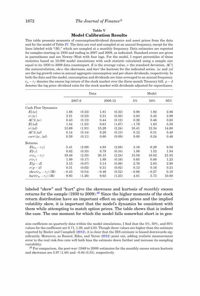
1872 The Journal of Finance R©
Table VModel Calibration Results
This table presents moments of consumption/dividend dynamics and asset prices from the dataand for the model of Table IV. The data are real and sampled at an annual frequency, except for thelines labeled with “(M),” which are sampled at a monthly frequency. Data estimates are reportedfor samples starting in 1930 and ending in 2007 and 2009, as indicated. Standard errors are givenin parentheses and are Newey–West with four lags. For the model, I report percentiles of thesestatistics based on 10,000 model simulations with each statistic calculated using a sample sizeequal to its 1930 to 2009 data counterpart. E is the average value, σ the standard deviation, AC1the autocorrelation, skew the skewness, and kurt the kurtosis for the indicated series. �c and �dare the log growth rates in annual aggregate consumption and per-share dividends, respectively. Inboth the data and the model, consumption and dividends are time-averaged to an annual frequency.rm − r f denotes the excess log return of the stock market over the three-month Treasury bill. p − ddenotes the log price–dividend ratio for the stock market with dividends adjusted for repurchases.
Data Model
2007.6 2009.12 5% 50% 95%
Cash Flow DynamicsE[�c] 1.88 (0.32) 1.81 (0.32) 0.98 1.92 2.86σ (�c) 2.21 (0.52) 2.21 (0.50) 2.03 2.45 2.99AC1(�c) 0.43 (0.12) 0.44 (0.12) 0.26 0.46 0.63E[�d] 1.54 (1.53) 0.61 (1.67) −1.79 1.83 5.50σ (�d) 13.69 (1.91) 15.29 (2.24) 10.41 12.34 14.60AC1(�d) 0.14 (0.14) 0.20 (0.13) 0.12 0.31 0.48corr(�c, �d) 0.59 (0.11) 0.60 (0.09) 0.00 0.24 0.46
ReturnsE[rm − r f ] 5.41 (2.09) 4.93 (2.08) 3.16 6.29 9.50E[r f ] 0.82 (0.35) 0.79 (0.34) 1.08 1.52 1.94σ (rm − r f ) 19.48 (2.35) 20.15 (2.24) 15.58 18.02 21.03σ (r f ) 1.89 (0.17) 1.89 (0.16) 0.65 0.88 1.23E[p − d] 3.15 (0.07) 3.14 (0.06) 2.76 2.83 2.90σ (p − d) 0.31 (0.02) 0.31 (0.02) 0.13 0.16 0.21skew(rm − r f ) (M) −0.43 (0.54) −0.46 (0.52) −0.86 −0.27 0.10kurt(rm − r f ) (M) 9.93 (1.26) 9.63 (1.23) 4.01 5.73 10.80
labeled “skew” and “kurt” give the skewness and kurtosis of monthly excessreturns for the sample (1930 to 2009).26 Since the higher moments of the stockreturn distribution have an important effect on option prices and the impliedvolatility skew, it is important that the model’s dynamics be consistent withthem while attempting to match option prices. The table shows that is indeedthe case. The one moment for which the model falls somewhat short is in gen-
sion coefficient on quarterly data within the model simulations, I find that the 5%, 50%, and 95%values for the coefficient are 0.71, 1.39, and 2.03. Though these values are higher than the estimatereported by Beeler and Campbell (2012), it is clear that the IES estimate is biased downwards sig-nificantly. Moreover, as Bansal, Kiku, and Yaron (2012) point out, adding realistic measurementerror to the real risk-free rate will both bias the estimate down further and increase its samplingvariability.
26 For comparison, the post-war (1949 to 2009) estimates for the monthly excess return kurtosisand skewness are 5.97 (1.48) and –0.84 (0.33), respectively.

Uncertainty, Time-Varying Fear, and Asset Prices 1873
Table VIVariance Premium
This table presents moments from the data and for the model of Table IV for conditional varianceand the variance premium (top panel) and regressions of excess stock market returns on thevariance premium (bottom panel). The data estimates are reported for the pre-crisis sample,1990.1 to 2007.6, and the full sample, 1990.1 to 2009.12, as indicated, and correspond to a monthlyfrequency. For the model, I report percentiles of these statistics based on 10,000 simulations, witheach statistic calculated using a sample size equal to its full-sample data counterpart. Standarderrors are given in parentheses and are Newey–West with four lags. VP is the variance premium,varP
t (rm) is the physical (i.e., true) forecast of return variance, and varQt (rm) is the risk-neutral
expectation of variance, which is given by VIX2. β(i) and R2(i) denote the slope coefficient and R2
for predictive regressions of excess stock market returns over horizons of i = 1, 3, and 6 monthson the lagged variance premium. For the regressions, excess returns are expressed as annualizedpercentages.
Data Model
2007.6 2009.12 5% 50% 95%
Variance PremiumE[VP] 11.05 (1.07) 10.55 (2.62) 5.75 8.17 13.01σ (VP) 7.63 (1.09) 8.47 (1.09) 3.40 7.53 16.31skew(VP) 2.43 (0.60) 2.19 (0.38) 1.54 2.69 4.31kurt(V P) 12.34 (3.52) 9.67 (2.09) 5.67 11.83 26.33AC1(varP
t (rm)) 0.82 (0.04) 0.81 (0.05) 0.76 0.85 0.92AC1(varQ
t (rm)) 0.79 (0.05) 0.82 (0.05) 0.75 0.84 0.92σ (varP
t (rm)) 17.41 (2.21) 31.00 (8.36) 8.83 14.97 29.80σ (varQ
t (rm)) 23.97 (3.15) 36.58 (8.07) 11.36 21.69 45.26skew(varQ
t (rm)) 2.02 (0.49) 3.38 (0.51) 0.88 2.19 3.75kurt(varQ
t (rm)) 8.98 (2.26) 19.21 (5.07) 3.96 9.18 21.23
Predictabilityβ(1) 0.74 (0.34) 0.80 (0.36) −0.09 1.10 2.65R2(1) 1.44 (1.48) 1.72 (1.64) 0.03 1.74 7.32β(3) 0.87 (0.25) 0.99 (0.25) −0.14 0.94 2.22R2(3) 6.15 (4.50) 6.93 (4.53) 0.06 3.91 16.93β(6) 0.51 (0.22) 0.76 (0.23) −0.22 0.75 1.78R2(6) 4.47 (4.77) 7.28 (5.33) 0.07 5.31 24.53
erating a large enough volatility for the price–dividend ratio. Comparing againthe pre-crisis and full-sample estimates, the table shows there is not muchdifference.
C.2. Variance Dynamics and Premium
Table VI provides statistics for integrated variance and the variance pre-mium, all at the monthly horizon. I focus first on a comparison of the modelwith the pre-crisis estimates and then discuss the full-sample moments. Notefirst that the model successfully generates a large average variance premium(E[V P]), comparable to that in the data. Hence, as in the data, index optionsin the model embed a high insurance premium. It is important to note that this

1874 The Journal of Finance R©
large premium is by no means implied by the fact that the model matches theequity premium or the level of return volatility. To illustrate this, I solve forthe variance premium implied by the calibrated model in Bansal, Kiku, andYaron (2007), a leading asset pricing model that successfully matches the eq-uity premium and high equity return volatility. I find that it is approximately0.35, which is far smaller than both the data and the values generated by themodel of this paper.
Table VI also shows that the model captures the high volatility of the con-ditional variance premium. This reflects the impact of time-variation in un-certainty concerns, as discussed in Section V. The table further shows thatthe model matches the high skewness and kurtosis of the variance premium,producing large values that are in line with the data. This is a result of spikesin the variance premium that arise due to jumps up in q2
t and the level ofuncertainty.
There is a tension between generating a large variance premium and re-maining consistent with the dynamics of conditional variance, which createsa challenge for models that confront both aspects of the data. The rest of thetop panel in Table VI demonstrates that the model respects the properties ofthe two conditional variance series, varP
t (rm) and varQt (rm) (i.e., VIX2). It shows
that the empirical autocorrelation estimates for these series are close to themedians of the simulated series, and easily within the 90% confidence inter-vals. Conditional variance is persistent, but not extremely so. The next twolines in the table show that the model is in line with the high volatility in theconditional variances themselves and matches the relatively higher volatilityin σ (varQ
t (rm)) compared to σ (varPt (rm)). The final two lines of the table show
that the squared VIX time series displays pronounced nonnormality, with alarge positive skewness and kurtosis. The model matches these features well.
Section II highlights the predictive ability of the variance premium for excessequity returns in the data. In the model, the variance premium is a good filterfor detecting fluctuations in the level of uncertainty. Since increases in uncer-tainty cause equity prices to fall and the expected return to rise, the variancepremium predicts excess equity returns within the model. The bottom panel ofTable VI shows that the model also captures this predictability quantitatively.It presents the projection coefficients in the data and in the model for predic-tive regressions of log excess returns on the variance premium for horizonsof one, three, and six months. As the table shows, the projection coefficientshave the right sign and the median values are roughly in line with the dataestimates. As in the data, the model-based R2s are quite large for these shorthorizons. The model median R2 for the one-month-ahead projection is roughly1.75% and the 90% finite sample distribution of R2 clearly includes the 1.44%R2 from the data. For the three- and six-month-ahead projections, the medianR2 increases to approximately 3.9% and 5.3% inside the model, which, thoughhigh, is similar to the 6.2% and 4.5% values in the data. Finally, in the modelthe variance premium is superior to the conditional variance as a predictorof equity returns, as first documented empirically by Bollerslev, Tauchen, andZhou (2009). This is due to the fact that, while both σ 2
t and q2t drive variation

Uncertainty, Time-Varying Fear, and Asset Prices 1875
in the conditional variance, variation in the equity risk premium comes mostlyfrom fluctuations in q2
t , which the variance premium captures cleanly.
C.3. Pre-Crisis and Full Samples
Comparing the pre-crisis and full-sample estimates, there is a striking in-crease in the volatility and higher moments of the conditional variance series.A large portion of this increase is due to October and November of 2008. Ex-cluding those two months, the estimates for σ (varP
t (rm)) and σ (varQt (rm)) are
22.6 and 29.5, respectively, while the skewness and kurtosis of varQt (rm) are
2.22 and 9.25, respectively. The changes in the other statistics in Table VIare less dramatic. The mean variance premium decreases from about 11 to10.5 and the volatility of the variance premium increases from 7.6 to around8.1. The very large realized variance in October and November of 2008 gener-ated a big positive payoff to the variance swap replication strategy discussedin Section II, reducing the estimate of the average premium paid by investorsfor this strategy. This reduction in the mean of VP was attenuated by the largevariance premium that prevailed in the following months, when uncertaintywas very high.
Note that the potential for a large change in the conditional variance mo-ments across the two samples is consistent with the calibration’s simulationpercentiles. The percentiles indicate that, for the given sample length, theseparticular moments have a wide sampling distribution under the model dueto the potential for large jump shocks. Notice that the full-sample estimatesfor the volatility and higher moments of the conditional variances are nearthe 95% of their model-based distributions. This is consistent with the crisis’svolatility dynamics representing a relative outlier for this sample length. Italso highlights the ability of the model to capture the possibility of this largechange in moments across the samples, providing evidence in favor of the modeldynamics. In contrast, the changes in the estimates are not consistent with therobust (HAC) standard errors for the pre-crisis sample, as most of the observedchanges in the estimates are by more than four standard errors. Compared tothe simulation percentiles, the robust standard errors are generally consistentfor the cash flow and return moments, but greatly underestimate the width ofthe sampling distributions for the variance dynamics. This observation is itselfalso consistent with the model, as shown in Table VII, which reports HAC stan-dard errors for the moment estimates computed within the model simulations.The table shows that HAC standard errors for the variance moments computedwithin the model are consistent with their empirical counterparts and tend tounderestimate the sampling distribution.
C.4. Option Prices and the Volatility Surface
Figure 2 displays plots comparing the empirical and model-based im-plied volatility curves for 1, 3, and 12-month maturities. These provide an

1876 The Journal of Finance R©
Table VIICalibration Results: Simulated HAC Standard Errors
This table presents the median HAC standard error corresponding to the given set of Monte Carlo(model-based) moments from Table VI. The sample of HAC standard errors is calculated from thesame samples used to generate the model-based statistics in Table VI. As with the data-basedstandard errors, which are given in the column labeled “Data,” the model-based HAC standarderrors are calculated using the Newey–West variance–covariance estimator with four lags. Symbolsare defined in Table VI.
Data Model2007.6 50%
VarianceE[VP] 1.07 0.94σ (VP) 1.09 1.40skew(VP) 0.60 1.60kurt(VP) 3.52 7.59σ (varP
t (rm)) 2.25 2.15σ (varQ
t (rm)) 3.14 3.54skew(varQ
t (rm)) 0.49 1.29kurt(varQ
t (rm)) 2.26 5.56
assessment of the model’s ability to fit the cross-sectional patterns in impliedvolatilities.27 To produce the model-based curves, I determine option prices forthe calibrated model and solve for their Black–Scholes implied volatilities. Asin the data, the options I price within the model are written on the equity priceindex excluding dividend payments (as opposed to a total return price index,which would include dividends). Option prices are calculated by first solvinga system of ODEs for the characteristic function of the state vector under theQ-measure, as in Duffie, Pan, and Singleton (2000). I next use this to computethe characteristic function of the price index and calculate and invert the optiontransform based on the method of Carr and Madan (1999). The plots presentthe model and empirical implied volatilities for strikes ranging in moneyness(Strike/Spot Price) from 0.75 to 1.25. This represents a very wide range ofstrikes for short-maturity options. The empirical implied volatilities are theaverage daily implied volatilities for options on the S&P 500 index traded inthe over-the-counter market. The data are obtained from Citigroup and coverOctober 1999 to June 2008.28 For the calculation of the model-based optionprices, the state vector Yt is set equal to its unconditional mean.
27 Note that fitting the implied volatility surface does not, by itself, imply that a model capturesthe variance premium. A model may violate aspects of the statistical (i.e., P-measure) distributionof returns while fitting the implied volatility surface. Matching the variance premium is a chal-lenging test for equilibrium models because it requires directly capturing the difference betweenthe P- and Q-measure distributions, that is, the “premium.”
28 The range of strikes available in the over-the-counter market for index options is often muchbroader than for exchange-traded options. See Foresi and Wu (2005) for more details on the over-the-counter market.

Uncertainty, Time-Varying Fear, and Asset Prices 1877
0.8
0.9
11.
11.
2
15202530354045
1-M
onth
Impl
ied
Vol
atili
ties
K/P
t (m
oney
ness
)
Implied Vol, %
data
mod
el
0.8
0.9
11.
11.
2
15202530354045
3-M
onth
Impl
ied
Vol
atili
ties
K/P
tImplied Vol, %
data
mod
el
0.8
0.9
11.
11.
2
15202530354045
1-Y
ear
Impl
ied
Vol
atili
ties
K/P
t (m
oney
ness
)
Implied Vol, %
data
mod
el
Fig
ure
2.O
ne-
,3-
,an
d12
-mon
thim
pli
edvo
lati
liti
es:
Mod
elan
dd
ata.
Th
efi
gure
plot
sco
mpa
riso
ns
ofem
piri
cal
and
mod
el-b
ased
impl
ied
vola
tili
ties
for
1-,3
-,an
d12
-mon
thm
atu
riti
es(l
eft,
cen
ter,
and
righ
tpl
ots,
resp
ecti
vely
)for
the
mod
elof
Tabl
eIV
.Str
ikes
are
expr
esse
din
mon
eyn
ess
(Str
ike
Pri
ce/S
pot
Pri
ce).
Th
eem
piri
calc
urv
esar
em
ean
sof
dail
yim
plie
dvo
lati
liti
esfo
rS
&P
500
inde
xop
tion
sfo
rth
epe
riod
1999
.10
to20
08.6
.Th
em
odel
-bas
edcu
rves
are
calc
ula
ted
for
opti
onpr
ices
obta
ined
wh
enth
em
odel
’sst
ate
vect
oris
set
equ
alto
its
un
con
diti
onal
mea
n.

1878 The Journal of Finance R©
The plots in Figure 2 show that the model does a good job matching boththe overall shape and the level of the implied volatility curves. In particular,it captures the skew, the steep slope in implied volatilities for otm puts. Modeluncertainty is instrumental in capturing this by increasing fears about the like-lihood and magnitude of adverse jump shocks, which result in negative returnsand generate a Q-measure return density with a heavy left tail. The impliedvolatility skew exists at all three maturities, but is particularly pronouncedfor the one-month maturity. The model captures the skew well at each of thethree maturities, and does a very nice job replicating the decay in the skewas the horizon increases. As can be seen by comparing across the plots, themodel further matches the shallow positive slope in the at-the-money impliedvols, whereby the 12-month at-the-money vol is the highest and the 1-monthvol the lowest. This is also clear from Figure IA.1 in the Internet Appendix,which displays separate plots of the empirical and model-based curves, furtherhighlighting the similarities in their appearance.
In addition to doing a good job matching the very steep slope in the one-monthimplied volatility curve at low moneyness strikes, the model also replicates thesmirk, the slight increase in implied volatility at high moneyness strikes. How-ever, it is apparent that the model-based curve does not dip as low as the empir-ical one. The same thing is true for the 3- and 12-month plots—the model fit isvery good for low moneyness strikes but not as good for high-moneyness strikes.
The Internet Appendix presents the results of a further exercise that use thedata on one-month implied volatilities. It displays the time series for q2
t andσ 2
t extracted by fitting the calibrated model each month to a set of one-monthimplied volatilities at different levels of moneyness. As reported there, thesample moments of the extracted time series are consistent with the momentsimplied by the model calibration.
D. The Impact of Uncertainty
As Section IV.B explains, the directions and magnitudes of the worst-casemodel perturbations depend on the equilibrium Acoefficients, which encode thesensitivity of the value function to perturbations. Under the worst-case model,cash flow growth is lower, the drift and persistence in volatility is increased,and the jump intensities and magnitudes are amplified. The overall impactof uncertainty on equilibrium asset prices depends on the combined interactedeffects of the worst-case perturbations. The comparative statics exercises belowevaluate this impact.
Table VIII conducts a two-part comparative statistics exercise on the cali-brated model by shutting off uncertainty with respect to parts of the model’sdynamics. The first panel, labeled Model 1-A, is for a model that shuts off un-certainty regarding only the jump shocks in the model, leaving on uncertaintyregarding the diffusive parts of the dynamics. Thus, the jumps are not per-turbed under the worst-case model. The second panel, Model 1-B, turns off allmodel uncertainty, so the investor has full confidence in the reference model.The table shows only the asset price data, since the cash flow dynamics beingsimulated are those of the reference model and therefore unaffected.
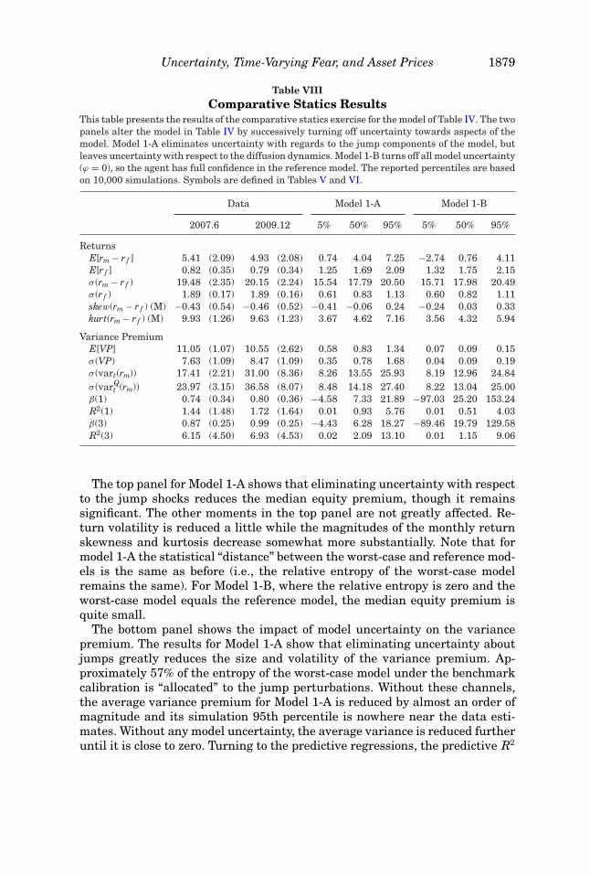
Uncertainty, Time-Varying Fear, and Asset Prices 1879
Table VIIIComparative Statics Results
This table presents the results of the comparative statics exercise for the model of Table IV. The twopanels alter the model in Table IV by successively turning off uncertainty towards aspects of themodel. Model 1-A eliminates uncertainty with regards to the jump components of the model, butleaves uncertainty with respect to the diffusion dynamics. Model 1-B turns off all model uncertainty(ϕ = 0), so the agent has full confidence in the reference model. The reported percentiles are basedon 10,000 simulations. Symbols are defined in Tables V and VI.
Data Model 1-A Model 1-B
2007.6 2009.12 5% 50% 95% 5% 50% 95%
ReturnsE[rm − r f ] 5.41 (2.09) 4.93 (2.08) 0.74 4.04 7.25 −2.74 0.76 4.11E[r f ] 0.82 (0.35) 0.79 (0.34) 1.25 1.69 2.09 1.32 1.75 2.15σ (rm − r f ) 19.48 (2.35) 20.15 (2.24) 15.54 17.79 20.50 15.71 17.98 20.49σ (r f ) 1.89 (0.17) 1.89 (0.16) 0.61 0.83 1.13 0.60 0.82 1.11skew(rm − r f ) (M) −0.43 (0.54) −0.46 (0.52) −0.41 −0.06 0.24 −0.24 0.03 0.33kurt(rm − r f ) (M) 9.93 (1.26) 9.63 (1.23) 3.67 4.62 7.16 3.56 4.32 5.94
Variance PremiumE[VP] 11.05 (1.07) 10.55 (2.62) 0.58 0.83 1.34 0.07 0.09 0.15σ (VP) 7.63 (1.09) 8.47 (1.09) 0.35 0.78 1.68 0.04 0.09 0.19σ (vart(rm)) 17.41 (2.21) 31.00 (8.36) 8.26 13.55 25.93 8.19 12.96 24.84σ (varQ
t (rm)) 23.97 (3.15) 36.58 (8.07) 8.48 14.18 27.40 8.22 13.04 25.00β(1) 0.74 (0.34) 0.80 (0.36) −4.58 7.33 21.89 −97.03 25.20 153.24R2(1) 1.44 (1.48) 1.72 (1.64) 0.01 0.93 5.76 0.01 0.51 4.03β(3) 0.87 (0.25) 0.99 (0.25) −4.43 6.28 18.27 −89.46 19.79 129.58R2(3) 6.15 (4.50) 6.93 (4.53) 0.02 2.09 13.10 0.01 1.15 9.06
The top panel for Model 1-A shows that eliminating uncertainty with respectto the jump shocks reduces the median equity premium, though it remainssignificant. The other moments in the top panel are not greatly affected. Re-turn volatility is reduced a little while the magnitudes of the monthly returnskewness and kurtosis decrease somewhat more substantially. Note that formodel 1-A the statistical “distance” between the worst-case and reference mod-els is the same as before (i.e., the relative entropy of the worst-case modelremains the same). For Model 1-B, where the relative entropy is zero and theworst-case model equals the reference model, the median equity premium isquite small.
The bottom panel shows the impact of model uncertainty on the variancepremium. The results for Model 1-A show that eliminating uncertainty aboutjumps greatly reduces the size and volatility of the variance premium. Ap-proximately 57% of the entropy of the worst-case model under the benchmarkcalibration is “allocated” to the jump perturbations. Without these channels,the average variance premium for Model 1-A is reduced by almost an order ofmagnitude and its simulation 95th percentile is nowhere near the data esti-mates. Without any model uncertainty, the average variance is reduced furtheruntil it is close to zero. Turning to the predictive regressions, the predictive R2

1880 The Journal of Finance R©
of the variance premium is reduced successively in the two models. When thejump intensity is not directly amplified under the worst-case model, as underModel 1-A, the jumps’ importance decreases along with the predictive powerof the variance premium. For Model 1-B, where there is no model uncertainty,the influence of q2
t on the equity risk premium is very small and so is itspredictive power. This is apparent in the diminished median R2s shown in thetable. Finally, as the variance premium becomes very small, the predictive re-gression coefficients become unstable. If the variance premium was this smallempirically, it would likely be obscured by estimation noise.
The results from the table are augmented by Figure 3, and also the InternetAppendix, which plot the implied volatility curves for Model 1-B. The figuresshow that the model-generated implied volatility curves are very flat and thatthe model does not capture the steep skew in implied volatility. This is partic-ularly apparent at the 1-month maturity, but is clearly also true for 3 and 12months.
As an additional exercise, I shut off all model uncertainty (as for Model 1-B)and raise risk aversion to the point where the equity premium matches thatof the benchmark calibration. The risk aversion required for this is 13.3. Forsuch a configuration the mean variance premium across simulations has a me-dian value of 4.23, and the median standard deviation of the variance premiumis 4.00. These numbers are only about half of their benchmark counterparts.Thus, in this case a high risk aversion alone is insufficient for jointly capturingthe variance and equity premiums. Moreover, a risk aversion of 13.3 alreadyexceeds the value 10, often considered the upper end of the reasonable rangefor risk aversion, and is substantially higher than the risk aversion of 5 used inthe benchmark calibration. Hence, for the benchmark calibration, model uncer-tainty, especially with regards to the jump shocks, is an important componentfor reconciling asset prices with fundamentals and a reasonable level of riskaversion.
Finally, Table IX looks at further comparative statics of the benchmark cal-ibration, obtained by changing ϕ and hence the detection-error probability ofthe worst-case model. The table shows the results for five values of ϕ, in in-creasing order, with the middle column (III) setting ϕ equal to its benchmarkcalibration value. Recall that increasing ϕ raises the level of model uncer-tainty, increasing the distance between the worst-case and reference modelsand hence decreasing the probability of detection error. For each ϕ the top rowsof the table show the detection-error probability of the worst-case model fordata samples of length 240, 480, and 720 months. The bottom panels reportasset pricing moments. Comparing across columns, the general patterns areclear. The equity premium increases and the risk-free rate decreases, as greateruncertainty makes the investor more concerned about lower cash flow growthrates and increased diffusive volatility and jump shocks. The joint impact ofthis uncertainty on variance expectations is shown by the variance premium,which increases sharply in the table. As the table shows, there is also a cor-responding, but smaller, increase in the volatility of conditional variance. Thisresults because, when the overall level of uncertainty is higher, variation in
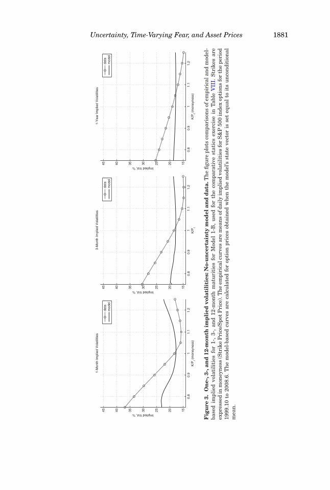
Uncertainty, Time-Varying Fear, and Asset Prices 1881
0.8
0.9
11.
11.
2
15202530354045
1-M
onth
Impl
ied
Vol
atili
ties
K/P
t (m
oney
ness
)
Implied Vol, %
data
mod
el
0.8
0.9
11.
11.
2
15202530354045
3-M
onth
Impl
ied
Vol
atili
ties
K/P
tImplied Vol, %
data
mod
el
0.8
0.9
11.
11.
2
15202530354045
1-Y
ear
Impl
ied
Vol
atili
ties
K/P
t (m
oney
ness
)
Implied Vol, %
data
mod
el
Fig
ure
3.O
ne-
,3-,
and
12-m
onth
imp
lied
vola
tili
ties
:No-
un
cert
ain
tym
odel
and
dat
a.T
he
figu
repl
ots
com
pari
son
sof
empi
rica
lan
dm
odel
-ba
sed
impl
ied
vola
tili
ties
for
1-,
3-,
and
12-m
onth
mat
uri
ties
for
Mod
el1-
B,
use
dfo
rth
eco
mpa
rati
vest
atic
sex
erci
sein
Tabl
eV
III.
Str
ikes
are
expr
esse
din
mon
eyn
ess
(Str
ike
Pri
ce/S
pot
Pri
ce).
Th
eem
piri
calc
urv
esar
em
ean
sof
dail
yim
plie
dvo
lati
liti
esfo
rS
&P
500
inde
xop
tion
sfo
rth
epe
riod
1999
.10
to20
08.6
.T
he
mod
el-b
ased
curv
esar
eca
lcu
late
dfo
rop
tion
pric
esob
tain
edw
hen
the
mod
el’s
stat
eve
ctor
isse
teq
ual
toit
su
nco
ndi
tion
alm
ean
.

1882 The Journal of Finance R©
Table IXChanging the Detection Error Probability
This table presents a comparison of the results for different levels of detection error probabilityfor the model of Table IV. The detection error probability is changed by varying the parameter ϕ
and is reported in the first three rows for samples of length T = 240, 480, and 720 months. Thereported values for the moments are the medians from 10,000 simulations of the model. The valuesof ϕ corresponding to columns I to V are 0.0024, 0.0038, 0.0048, 0.0053, and 0.0058, respectively.Symbols are defined in Tables V and VI.
I II III IV VStatistic (50%) (50%) (50%) (50%) (50%)
Sample Size / D.E. Prob.T = 240 months 0.323 0.282 0.261 0.252 0.246T = 480 months 0.244 0.192 0.164 0.152 0.142T = 720 months 0.194 0.137 0.109 0.097 0.088
E[rm − r f ] 3.90 5.18 6.29 7.16 8.51E[r f ] 1.69 1.62 1.52 1.45 1.33skew(rm − r f ) (M) −0.06 −0.16 −0.27 −0.36 −0.56kurt(rm − r f ) (M) 4.62 5.08 5.73 6.21 7.50E[V P] 1.85 4.29 8.17 11.92 19.37σ (V P) 1.75 4.04 7.53 11.10 18.31σ (vart(rm)) 13.41 14.07 14.97 15.83 17.15σ (varQ
t (rm)) 14.77 17.46 21.69 25.99 34.42R2(1) 0.98 1.40 1.74 2.04 2.72R2(3) 2.23 3.08 3.91 4.63 6.27
the drivers of uncertainty also induce a stronger reaction in equity prices. Thevolatility of uncertainty shocks is then a more important driver of conditionalvariance and increases its overall volatility. When the uncertainty level issubject to jump shocks, as is the case here, then this also leads to a fatter tailin returns. This is apparent in the table, where, for higher levels of uncertainty,there is a more negative return skewness and greater kurtosis. In addition, thegreater impact of uncertainty variation on equity prices leads to greater pre-dictability of equity returns by the variance premium, as evidenced in the lasttwo lines of the table.
VII. Conclusion
This paper builds an equilibrium model where the representative investor isconcerned about a rich set of alternative models of the economy. The investor’sattempt to hedge his model uncertainty optimally focuses his concerns on as-pects of his model for which an error would be harmful to his utility while alsobeing difficult to detect in the data. I solve for the investor’s worst-case modeland for equilibrium asset prices. I show that model uncertainty concerns help tocapture the large premium contained in the prices of equity index options, andthat variation in this option premium reflects variation in the level of model

Uncertainty, Time-Varying Fear, and Asset Prices 1883
uncertainty. This implies that the option premium should predict excess stockreturns, consistent with the empirical results I present.
I present a calibrated specification of this model and show that with a statis-tically reasonable level of model uncertainty it is able to jointly capture salientmoments of cash flows, equity returns, the risk-free rate, variance dynamics,and the large equity index option premium. Moreover, the model generates arealistic implied volatility surface. I demonstrate that model uncertainty hasa large impact on the model’s asset prices, especially the variance premium,which is impacted strongly by uncertainty concerns about the frequency andmagnitude of jump shocks.
Introspection suggests that Knightian uncertainty is an important factor indecision making. Hence, model uncertainty can be an important channel inmacroeconomic and financial models. There has also been a lot of discussionsuggesting that Knightian uncertainty, the “unknown unknowns,” was an influ-ential factor in the recent economic crises. The plots of the model uncertaintyproxy and estimated option premium presented in this paper are consistentwith this notion and closely track the timeline of the crises. It therefore seemsfruitful for future research to expand on the work here and in related studiesto improve our understanding of the role of model uncertainty in macrofinancemodels.
Initial submission: April 27, 2010; Final version received: April 25, 2013Editor: Campbell Harvey
Appendix A: Derivation of Relative Entropy Growth
As discussed in the main text, the relative entropy growth rate is defined as
R(ηt) = dds |s=0
Eηt [ln ηt+s].
Since ηt = ηdZt ηJ
t , we can compute the relative entropy growth rate of the dif-fusion and jump parts separately and then add them. Furthermore, we candetermine R(ηJ
t ) by adding the relative entropy growth rates of the componentjumps.
To determine R(ηdZt ), write ln ηdZ
t in terms of Zηt rather than Zt (see Internet
Appendix Section III. We then have that ln ηdZt+s = 1
2
∫ t+st hT
u hudu + ∫ t+st hT
u dZηu.
Since the second term is a martingale under P(η), its time-t expectation is zero.It is thus clear that
R(ηdZ
t
) = 12
hTt ht.
Now consider R(ηJit ), where ηJi is the term in ηt that changes the probability
law for the gamma-distributed jumps (from Internet Appendix Section III). Tofind R(ηJi
t ), recall two facts: (1) lηt = exp(a)lt and (2) Eηt [ξi] = kθ
1−θb . Using these

1884 The Journal of Finance R©
facts, a straightforward calculation shows that
R(η
Jit
) = exp(a)lt
(a + b
kθ
1 − θb+ k ln(1 − θb) − 1
)+ lt.
Finally, consider R(ηJkt ), where ηJk is the term in ηt that changes the
probability law for the normally distributed jumps (from Internet AppendixSection III). Straightforward calculations and algebraic simplification showthat
R(η
Jkt
) = exp(a)lt
(a + 1
2�μ2
σ 2 + 12
sσ − 12
ln sσ − 32
)+ lt.
Appendix B: HJB Equation Derivation
Substituting (6) into the aggregator (5) gives
f (Ct, Jt) = δ exp(γ g(Yt) + γ ln Ct)
[exp(−ρg(Yt)) − 1
ρ
].
Using Ito’s lemma, we have that
Et[dJc] = JTY μ(Yt)dt + 1
2tr[JY Y �(YT )�(Yt)T ]dt,
where the superscript “c” denotes the continuous (diffusive) part of the dy-namics and tr denotes the trace operator. For notational convenience, letG(Yt) = g(Yt) + ln Ct, so that we can write J(Yt) = exp(γ G(Yt))/γ . Further-more, let GY (Yt) and GY Y (Yt) denote the gradient and Hessian matrix ofG(Yt). Then JY = exp(γ G(Yt))GY (Yt) and JY Y = exp(γ G(Yt))
[γ GY GT
Y + GY Y].
The Hamilton-Jacobi-Bellman (HJB) equation (4) can then be rewritten as
0 = minP(ηt)
δ
ρexp(γ G(Yt))[exp(−ρg(Yt)) − 1] + exp(γ G(Yt))GT
Y μ(Yt)
+ exp(γ G(Yt))GTY2
�2,th2,t + 12
exp(γ G(Yt))tr[γ GT
Y �t�Tt GY + GY Y �t�
Tt
]+ 1
γEη
t [exp(γ G(Yt− + ξt · dNt)) − exp(γ G(Yt−))]
s.t. R(ηt) ≤ ϕq2t , (B1)
where the arguments of the derivatives have been omitted to reduce clutter.Note that the term �2,th2,t is due to the drift perturbation under P(η) and thatGY2 just denotes the derivative of G(Y ) with respect to Y2,t.

Uncertainty, Time-Varying Fear, and Asset Prices 1885
Appendix C: Proof of Proposition 1
The first step is to substitute the conjecture g(Yt) = A0 + A′Yt into theexpanded HJB equation (B1) derived in Appendix B. To facilitate this, let Adenote the vector obtained by augmenting A with a component equal to one, sothat δ′
c A = 1. Then we can concisely write G(Yt) = A0 + A′Yt. Moreover, we seethat GY = A and GY Y = 0. In addition, let A = [A1, A2]′ be partitioned in thesame way as Y = [Y1, Y2]′. Then we can write GY2 = A2. We can substitute infor the diffusion terms in (B1). For the jump terms, we have
1γ
Eηt [exp(γ G(Yt− + ξt · dNt)) − exp(γ G(Yt−))]
= exp(γ G(Yt))γ
Eηt [exp(γ A′(ξt · dNt)) − 1]
= exp(γ G(Yt))γ
lηt′(ψη(γ A) − 1),
where, as before, ψη(γ A) denotes the stacked vector of P(η)-measure moment-generating functions evaluated componentwise at the vector γ A. I write outthe functional form of these moment-generating functions for the two types ofjumps considered, normal jumps and gamma jumps. Let ξi and ξk be the gammaand normally distributed jumps, respectively. As shown in Internet AppendixSection III under P(η) we have ξi ∼ (k, θ
1−θb) and ξk ∼ N (μ + �μ, σ 2sσ ). There-
fore, ψη
i (γ Ai) = (1 − θγ Ai1−θb)−k and ψ
η
k (γ Ak) = exp(γ Ak(μ + �μ) + 12γ 2 A2
kσ2sσ ).
Substituting the derived expressions into (B1) and factoring out the termexp(γ G(Yt)) gives
0 = minP(ηt)
exp(γ G(Yt)) ×{
δ
ρ[exp(−ρg(Yt)) − 1] + A
′μ(Yt) + A2
′�2,th2,t (C1)
+ 12
γ A′�t�
Tt A+ 1
γlηt
′(ψη(γ A) − 1)}
s.t. R(ηt) ≤ ϕq2t .
We can now proceed with the minimization. Let λt be the Lagrange multiplieron the constraint R(ηt) ≤ ϕq2
t . The functional form of R(ηt) in terms of the worst-case parameters is given by the sum of the expressions in Appendix A. Thefirst-order conditions for the minimization are taken with respect to the theworst-case model parameters (h2,t, a,�u, sσ , b). They are:
FOC(h2,t) : exp(γ G(Yt))�′2,t A2 + λth2,t = 0
FOC(�μ) : exp(γ G(Yt))1γ
lηt,k∂
∂�μψη(γ Ak) + λt
∂
∂�μR(ηJk
t ) = 0
FOC(sσ ) : exp(γ G(Yt))1γ
lηt,k∂
∂sσ
ψη(γ Ak) + λt∂
∂sσ
R(ηJkt ) = 0

1886 The Journal of Finance R©
FOC(b) : exp(γ G(Yt))1γ
lηt,i∂
∂bψη(γ Ai) + λt
∂
∂bR(ηJi
t ) = 0
FOC(a) : exp(γ G(Yt))1γ
exp(a)lt ′(ψη(γ A) − 1) + λt∂
∂aR(ηt) = 0.
Moreover, the entropy constraint binds, which adds the equation R(ηt) = ϕq2t .
For a given value of the vector A, these equations fix the values of the worst-caseparameters. To solve the system, I conjecture that λt = λ exp(γ G(Yt)), whereλ > 0 is a constant that defines the part of the Lagrange multiplier that isstate-independent. By substituting this conjecture into the above system, I candivide through by exp(γ G(Yt)) in each of the equations and cancel the state-dependent terms exp(γ G(Yt)) and λt, leaving the constant λ.
Solving the first equation, we obtain h2,t = − 1λ�′
2,t A2. This implies that theperturbation in the model drift is �2,th2,t = − 1
λHq A2q2
t and the contribution ofht to R(ηt) is 1
2 h′tht = 1
21λ2 A′
2 Hq A2q2t . Thus, the drift perturbation is proportional
to q2t and the perturbation’s cost in terms of entropy is also proportional to
q2t . This expression for the drift’s entropy cost can now be substituted into the
entropy constraint and we can eliminate the first-order condition for h2,t fromthe above system.
The remaining issue for solving this system is the dependence of a number ofterms on the level of q2
t . As just shown, the term 12 h′
tht in the entropy constraintis proportional to q2
t . Furthermore, the jump intensity lt, which is proportionalto q2
t , appears in the other first-order conditions. It appears both explicitly onthe left side of each equation and implicitly in the partial derivatives of R(the expression for R is in Appendix A). This means that all of the remainingequations are in fact proportional to q2
t and so q2t can be canceled out from all of
them. The resulting equation system is now completely state-independent andhas as its solution the constant vector of worst-case parameters (a,�u, sσ , b)and λ.
The remaining step is to find the equations determining the value of thevector A and in the process verify the conjectured solution for g(Yt). Towardthat end, I approximate the term exp(−ρg(Yt)) in (C1) via a log-linearization.As the Internet Appendix shows, exp(−ρg(Yt)) is just 1
δtimes the equilibrium
consumption-wealth ratio. I follow Campbell et al. (2004) and log-linearize itaround the unconditional mean of the equilibrium log consumption-wealth ra-tio as follows: exp(−ρg(Yt)) ≈ κ0 + κ1ρg(Yt), where κ1 = − exp(−ρE[g(Yt)]) andκ0 = −κ1(1 + ρE[g(Yt)]) = −κ1(1 − ln(−κ1)). Note that the values of κ0 and κ1are endogenous to the equilibrium solution of the model. As Campbell et al.(2004) point out, this property of the approximation is important in obtain-ing accuracy over a range of values for ψ and γ . Furthermore, L’Hospital’srule gives that limρ→0
exp(−ρg(Yt))−1ρ
= −g(Yt) = limρ→0κ0+κ1ρg(Yt)−1
ρ, so the ap-
proximation to the PDE becomes exact as ρ → 0 (ψ → 1). Substituting in thisapproximation and the functional form of g(Yt), the first term in (C1) becomesδ( κ0−1
ρ+ κ1 A0) + δκ1 A′Yt.
Uncertainty, Time-Varying Fear, and Asset Prices 1887
Given the worst-case model parameters, (C1) must hold for all values ofYt. The solution to this equation determines the values of A and A0 and ver-ifies the conjectured solution for g(Yt). As Yt is (n − 1)-dimensional, the sys-tem of equations is n-dimensional, one equation for each of the (n − 1) ele-ments in Yt and one for the constant terms. Expanding out (C1) (and using thelog-linearization), we get the following system:
0 = δ
ρ(κ0 + κ1ρ A0 − 1) + AT μ
0 = Y Tt Aδκ1 + Y T
t KT A− 1λ
(AT
2 Hq A2)q2
t + 12
γ AT �t�Tt A
+ 1γ
lη1′(ψη(γ A) − 1)q2
t . (C2)
Combining these equations with the first-order conditions above and theequations defining κ0 and κ1 gives the system of equations that defines theequilibrium solution. The solution can be found numerically and verifiesthe conjectured functional form for the value function.
REFERENCES
Andersen, Torben G., Tim Bollerslev, and Francis X. Diebold, 2007, Roughing it 4p: Includingjump components in the measurement, modeling, and forecasting of return volatility, Reviewof Economics and Statistics 89, 701–720.
Andersen, Torben G., Tim Bollerslev, Francis X. Diebold, and Heiko Ebens, 2001, The distributionof stock return volatility, Journal of Financial Economics 61, 43–76.
Anderson, Evan W., Eric Ghysels, and Jennifer L. Juergens, 2009, The impact of risk and uncer-tainty on expected returns, Journal of Financial Economics 94, 233–363.
Anderson, Evan W., Lars P. Hansen, and Thomas J. Sargent, 2003, A quartet of semigroups formodel specification, robustness, prices of risk, and model detection, Journal of the EuropeanEconomic Association 1, 68–123.
Avramov, Doron, 2002, Stock return predictability and model uncertainty, Journal of FinancialEconomics 64, 423–458.
Avramov, Doron, 2004 Stock return predictability and asset pricing models, Review of FinancialStudies 17, 699–738.
Backus, David, Mikhail Chernov, and Ian Martin, 2011, Disasters implied by equity index options,Journal of Finance 66, 1969–2012.
Bakshi, Gurdip, and Nikunj Kapadia, 2003, Delta-hedged gains and the negative volatility riskpremium, Review of Financial Studies 16, 527–566.
Bansal, Ravi, Robert F. Dittmar, and Christian Lundblad, 2005, Consumption, dividends, and thecross-section of equity returns, Journal of Finance 60, 1639–1672.
Bansal, Ravi, Dana Kiku, and Amir Yaron, 2007, Risks for the long run: Estimation and inference,Working paper, The Wharton School, University of Pennsylvania.
Bansal, Ravi, Dana Kiku, and Amir Yaron, 2012, An empirical evaluation of the long-run risksmodel for asset prices, Critical Finance Review 1, 183–221.
Bansal, Ravi, and Amir Yaron, 2004, Risks for the long run: A potential resolution of asset pricingpuzzles, Journal of Finance 59, 1481–1509.
Barillas, Francisco, Lars Hansen, and Thomas Sargent, 2009, Doubts or variability? Journal ofEconomic Theory 144, 2388–2418.

1888 The Journal of Finance R©
Barro, Robert J., 2006, Rare disasters and asset markets in the twentieth century, QuarterlyJournal of Economics 121, 823–867.
Bates, David S., 2003, Empirical option pricing: A retrospection, Journal of Econometrics 116,387–404.
Beeler, Jason, and John Y. Campbell, 2012, The long-run risks model and aggregate asset prices:An empirical assessment, Critical Finance Review 1, 141–182.
Ben-David, Itzhak, John R. Graham, and Campbell R. Harvey, 2010, Managerial miscalibration,Working paper, The Ohio State University and Duke University.
Benzoni, Luca, Pierre Collin-Dufresne, and Robert S. Goldstein, 2011, Explaining asset pricingpuzzles associated with the 1987 market crash, Journal of Financial Economics 101, 552–573.
Bollerslev, Tim, Michael Gibson, and Hao Zhou, 2011, Dynamic estimation of volatility risk premiaand investor risk aversion from option-implied and realized volatilities, Journal of Economet-rics 160, 102–118.
Bollerslev, Tim, George Tauchen, and Hao Zhou, 2009, Expected stock returns and variance riskpremia, Review of Financial Studies 22, 4463–4492.
Brennan, Michael J., and Yihong Xia, 2001, Stock price volatility and equity premium, Journal ofMonetary Economics 47, 249–283.
Brevik, Frode, 2008, State uncertainty aversion and the term structure of interest rates, Workingpaper, VU Amsterdam.
Britten-Jones, Mark, and Anthony Neuberger, 2000, Option prices, implied price processes, andstochastic volatility, Journal of Finance 55, 839–866.
Broadie, Mark, Mikhail Chernov, and Michael Johannes, 2007, Model specification and risk pre-miums: Evidence from futures options, Journal of Finance 62, 1453–1490.
Campbell, John Y., George Chacko, Jorge Rodriguez, and Luis M. Viceira, 2004, Strategic assetallocation in a continuous-time VAR model, Journal of Economic Dynamics and Control 28,2195–2214.
Campbell, John Y., and John H. Cochrane, 1999, By force of habit: A consumption-based explana-tion of aggregate stock market behavior, Journal of Political Economy 107, 205–255.
Campbell, John Y., and Robert Shiller, 1988, Stock prices, earnings, and expected dividends,Journal of Finance 43, 661–676.
Carr, Peter, and Dilip Madan, 1999, Option valuation using the fast Fourier transform, Journalof Computation Finance 2, 61–73.
Carr, Peter, and Liuren Wu, 2009, Variance risk premiums, Review of Financial Studies 22, 1311–1341.
Coval, Joshua D., and Tyler Shumway, 2001, Expected option returns, Journal of Finance 56,983–1010.
Demeterfi, Kresimir, Emanuel Derman, Michael Kamal, and Joseph Zou, 1999, A guide to volatilityand variance swaps, Journal of Derivatives 6, 9–32.
Drechsler, Itamar, and Amir Yaron, 2011, What’s vol got to do with it, Review of Financial Studies24, 1–45.
Du, Du, 2010, General equilibrium pricing of options with habit formation and event risks, Journalof Financial Economics 99, 400–426.
Duffie, Darrell, and Larry G. Epstein, 1992, Stochastic differential utility, Econometrica 60, 353–394.
Duffie, Darrell, Jun Pan, and Kenneth J. Singleton, 2000, Transform analysis and asset pricingfor affine jump-diffusions, Econometrica 68, 1343–1376.
Epstein, Larry G., and Martin Schneider, 2003, Recursive multiple-priors, Journal of EconomicTheory 113, 1–31.
Epstein, Larry G., and Stanley E. Zin, 1989, Substitution, risk aversion, and the intertemporalbehavior of consumption and asset returns: A theoretical framework, Econometrica 57, 937–969.
Eraker, Bjorn, 2004, Do equity prices and volatility jump? Reconciling evidence from spot andoption prices, Journal of Finance 56, 1367–1403.
Eraker, Bjorn, and Ivan Shaliastovich, 2008, An equilibrium guide to designing affine pricingmodels, Mathematical Finance 18, 519–543.

Uncertainty, Time-Varying Fear, and Asset Prices 1889
Foresi, Silverio, and Liuren Wu, 2005, Crash-o-phobia: A domestic fear or worldwide concern?,Journal of Derivatives 13, 8–21.
Hansen, Lars, and Thomas Sargent, 2010, Fragile beliefs and the price of model uncertainty,Quantitative Economics 1, 129–162.
Hansen, Lars P., and Thomas J. Sargent, 2008, Robustness (Princeton University Press, Princeton,NJ).
Hansen, Lars P., Thomas J. Sargent, Gauhar A. Turmuhambetova, and Noah Williams, 2006,Robust control and model misspecification, Journal of Economic Theory 128, 45–90.
Hansen, Peter R., and Asger Lunde, 2006, Realized variance and market microstructure noise,Journal of Business and Economics Statistics 24, 127–161.
Jiang, George, and Yisong Tian, 2005, Model-free implied volatility and its information content,Review of Financial Studies 18, 1305–1342.
Kleshchelski, Isaac, and Nicolas Vincent, 2007, Robust equilibrium yield curves, Working paper,Northwestern.
Liu, Jun, Jun Pan, and Tan Wang, 2005, An equilibrium model of rare-event premia and itsimplication for option smirks, Review of Financial Studies 18, 131–164.
Maenhout, Pascal J., 2004, Robust portfolio rules and asset pricing, Review of Financial Studies17, 951–983.
Maenhout, Pascal J., 2006, Robust portfolio rules and detection error probabilities for a mean-reverting risk premium, Journal of Economic Theory 128, 136–163.
Mehra, Rajnish, and Edward C. Prescott, 1985, The equity premium: A puzzle, Journal of MonetaryEconomics 15, 145–161.
Menzly, Lior, Tano Santos, and Pietro Veronesi, 2004, Understanding predictability, Journal ofPolitical Economy 112, 1–47.
Pan, Jun, 2002, The jump-risk premia implicit in options: Evidence from an integrated time- seriesstudy, Journal of Financial Economics 63, 3–50.
Pastor, Lubos, 2000, Portfolio selection and asset pricing models, Journal of Finance 55, 179–223.Pastor, Lubos, and Robert Stambaugh, 2000, Comparing asset pricing models: An investment
perspective, Journal of Financial Economics 56, 335–381.Pastor, Lubos, and Robert Stambaugh, 2011, Are stocks really less volatile in the long run?, Journal
of Finance 67, 431–478.Rubinstein, Mark, 1994, Implied binomial trees, Journal of Finance 69, 771–818.Shaliastovich, Ivan, 2011, Learning, confidence, and option prices, Working paper, Wharton School,
University of Pennsylvania.Singleton, Kenneth, 2006, Empirical Dynamic Asset Pricing (Princeton University Press, Prince-
ton, NJ).Todorov, Viktor, 2010, Variance risk premium dynamics: The role of jumps, Review of Financial
Studies 23, 345–383.Trojani, Fabio, and Alessandro Sbuelz, 2008, Asset prices with locally-constrained-entropy recur-
sive multiple priors utility, Journal of Economic Dynamics and Control 32, 3695–3717.Ulrich, Maxim, 2013, Inflation ambiguity and the term structure of U.S. Government bonds,
Journal of Monetary Economics 60, 295–309.Uppal, Raman, and Tan Wang, 2003, Model misspecification and underdiversification, Journal of
Finance 58, 2465–2486.Veronesi, Pietro, 2000, How does information quality affect stock returns? Journal of Finance 55,
807–837.