Master of Science thesis in meteorology

UNCERTAINTY IN FOREST-ATMOSPHERE EXCHANGE OF ENERGY AND CARBON DIOXIDE BASED ON

TWO VERTICALLY DISPLACED EDDY COVARIANCE SET-UPS

Lauri Heiskanen

18.5.2017

Supervisors: Prof. Timo Vesala, Dos. Ivan Mammarella, Dos. Üllar Rannik,

Dr. Pasi Kolari, Dr. Olli Peltola

Examiners: Prof. Timo Vesala, Dos. Ivan Mammarella

UNIVERSITY OF HELSINKI DEPARTMENT OF PHYSICS

POB 64 (Gustaf Hällströmin katu 2)

00014 University of Helsinki

HELSINGIN YLIOPISTO – HELSINGFORS UNIVERSITET – UNIVERSITY OF HELSINKI Tiedekunta/Osasto – Fakultet/Sektion – Faculty/Section

Matemaattis-luonnontieteellinen tiedekunta Laitos – Institution – Department

Fysiikan laitos Tekijä – Författare – Author

Lauri Heiskanen Työn nimi – Arbetets titel – Title

Pyörrekovarianssimenetelmällä mitattujen mäntymetsän ja ilmakehän välisen hiilidioksidi- sekä

energiavoiden epävarmuustekijät Oppiaine – Läroämne – Subject

Meteorologia Työn laji – Arbetets art – Level

Pro gradu -tutkielma Aika – Datum – Month and year 18.5.2017

Sivumäärä – Sidoantal – Number of pages 50

Tiivistelmä – Referat – Abstract

Tässä Pro gradu -tutkielmassa tutkitaan pyörrekovarianssimenetelmällä mitattujen suomalaisen

mäntymetsän ja ilmakehän välisen hiilidioksidin, vesihöyryn sekä havaittavan lämmön voita, ja

pyritään selvittämään mittauksiin liittyvien virhelähteiden suuruudet. Voihin liittyvien virheiden

suuruutta analysoidaan vertailemalla saman mittaustornin kahdelta eri korkeudelta saatuja

mittaustuloksia. Analyysissa pyritään identifioimaan mikäli tuloksissa havaittavat eroavaisuudet

aiheutuvat mikrometeorologisista ja biologisista muuttujista vai turbulenttisten virtausten

kaoottisuudesta johtuvista mittausvirheistä. Pyörrekovarianssimenetelmän virhelähteet ovat osana

aktiivista tieteellistä keskustelua, jossa pyritään parantamaan meteorologisia mittausmenetelmiä.

Tutkimus tehtiin käyttämällä meteorologista aineistoa sekä vuoaineistoa, joka on kerätty Hyytiälän

SMEAR II -metsäntutkimusasemalla vuonna 2015. Mittaukset tehtiin 23,3 m sekä 33,0 m korkeudella

maanpinnasta. Vuoaineistoa tarkastellaan aina päivittäisestä vaihtelusta koko vuoden kestävään

kumulatiiviseen analyysiin. Aineistolle tehdään myös sekä meteorologisiin muuttujiin että

kasvillisuusjakaumaan perustuva tarkastelu.

Tutkimuksessa havaittiin mittauskorkeuksien välisen kumulatiivisten hiilidioksidivoiden eron

suuruudeksi 49 gC m−2 vuodessa (17 % erotus). Kokonaishaihdunnan kumulatiivisen eron arvioidaan

olevan 105 mm vuodessa (29 % erotus). Havaittavan lämmön voissa ei ilmennyt merkittävää eroa

mittauskorkeuksien välillä.

Hiilidioksidivuossa tai havaittavan lämmön vuossa ei havaita merkittävää eroa, joka aiheutuisi

käytettävistä mittauskorkeuksista. Kuitenkin latentin lämmön vuossa ero on havaittavissa, sillä 33,0 m

mittaustulokset ovat jatkuvasti pienempiä kuin 23,3 m vastaavat tulokset.

Avainsanat – Nyckelord – Keywords

Pyörrekovarianssi, pohjoinen havumetsä, hiilidioksidivuo, latentin lämmön vuo, havaittavan lämmön

vuo, footprint analyysi Säilytyspaikka – Förvaringställe – Where deposited

Kumpulan tiedekirjasto Muita tietoja – Övriga uppgifter – Additional information

HELSINGIN YLIOPISTO – HELSINGFORS UNIVERSITET – UNIVERSITY OF HELSINKI Tiedekunta/Osasto – Fakultet/Sektion – Faculty/Section

Faculty of Science Laitos – Institution – Department

Department of Physics Tekijä – Författare – Author

Lauri Heiskanen Työn nimi – Arbetets titel – Title

Uncertainty in forest-atmosphere exchange of energy and carbon dioxide based on two vertically

displaced eddy covariance set-ups Oppiaine – Läroämne – Subject

Meteorology Työn laji – Arbetets art – Level

Master’s thesis Aika – Datum – Month and year 18.5.2017

Sivumäärä – Sidoantal – Number of pages

50 Tiivistelmä – Referat – Abstract

This thesis is a study of the uncertainties related to the eddy covariance measurement technique on a

forest ecosystem that is located in Hyytiälä, Southern Finland. The aim of this study is to analyze

carbon dioxide and energy fluxes measured at two vertically displaced eddy covariance set-ups. In

particular, to determine if the observed deviations between the set-ups could be linked with

micrometeorological or biological variations or if they are resulted just by the stochastic nature of

turbulence. The magnitude of uncertainties linked to eddy covariance technique are still under

discussion and this thesis attempts to shed a light on these questions.

The analysis is done to half hourly mean flux and meteorological data that was measured at the

Hyytiälä SMEAR II –site in 2015 at the heights of 23.3 m and 33.0 m. Monthly, diurnal and

cumulative variations of the fluxes are analyzed. A footprint model is used to analyze the flux

correlation with the underlying vegetation. The flux dependence on atmospheric stability is also

determined.

The analysis shows that the annual cumulative difference of net ecosystem exchange (CO2 exchange)

between the two measurement heights is estimated to be 49 gC m−2year−1 (17 % difference). The

annual cumulative evapotranspiration difference is estimated to be 105 mm (29 % difference). There

are no significant differences between the sensible heat fluxes.

The difference between the measurement heights does not seem to influence significantly the flux

estimations made with the eddy covariance method. However, the measurement results for latent heat

flux acquired from the 33.0 m set-up are continuously smaller than those of the 23.3 m set-up.

Avainsanat – Nyckelord – Keywords

Eddy covariance, boreal forest, carbon dioxide flux, latent heat flux, sensible heat flux, flux footprint Säilytyspaikka – Förvaringställe – Where deposited

Kumpula Science Library Muita tietoja – Övriga uppgifter – Additional information

CONTENTS

1 INTRODUCTION 1

2 THEORY 3

2.1 Atmospheric boundary layer 3

2.1.1 Atmospheric turbulence 5

2.1.2 Diurnal cycle 6

2.2 Vertical turbulent transport in the surface layer 7

2.2.1 Reynolds decomposition 7

2.2.2 Surface fluxes 8

2.3 Eddy covariance method 9

2.3.1 Friction velocity and stability parameter 11

2.4 Footprint 12

2.5 Flux partitioning 13

3 MATERIALS AND METHODS 13

3.1 Site info 13

3.2 Measurement set-up 14

3.3 Data post processing 16

3.3.1 Friction velocity filtering 16

3.3.2 Gap filling 17

4 RESULTS 18

4.1 Monthly variation 19

4.2 Diurnal variation 27

4.3 Differences due to wind direction 32

4.4 Differences due to atmospheric stability 33

4.5 Footprint analysis 39

4.6 Cumulative ecosystem exchange 43

5 CONCLUSIONS 46

REFERENCES

1 INTRODUCTION

Reliable data collection of the micrometeorological and biological processes is

crucial in mitigating the effects of the climate change. Accurate measurement records

of the carbon sources and sinks in different ecosystems aids us to understand the

repercussions of the human-induced greenhouse gas emissions. The improvements in

micrometeorological measurement technology in the last decades has enabled us to

have continuous measurements from the rapid fluctuations to interannual variability

of the meteorological variables (Baldocchi, 2003). The eddy covariance (EC) method

is able to meet the needed requirements of reliable data collection and is utilized in

many meteorological measurements.

The eddy covariance technique is widely used and approved measurement method

that gives valuable estimates of the ecosystem-atmosphere exchange of greenhouse

gasses and energy fluxes (Aubinet et al. 2012). The EC technique is able to measure

the ecosystem-atmosphere fluxes from the turbulent motion of air. However, the

level of uncertainty of the measurement results is still under discussion and studied.

While utilizing the EC method, some assumptions and simplifications must be made,

which may cause uncertainties to the results.

If the underlying theoretical assumptions of the EC method are not fully met at the

measurement site, the EC method itself creates some systematical uncertainty to the

results. To tackle this problem, the requirements are always taken into serious

consideration during the measurement site assembly. The ecosystem should be

homogeneous, which includes flat topography and uniform roughness elements

(Aubinet et al. 2012). However, many sites, like the measurement station analyzed in

this thesis, do not have complete homogeneity in all directions. For instance, forests

and their canopies are not completely homogeneous surfaces neither in terms of gas

exchange nor topography. Other uncertainties related to the theoretical assumptions

are thought to be caused by inaccurate nighttime flux measurements as the emissions

escape through other transport routes closer to the ground, while never reaching the

measurement height (Aubinet et al., 2000).

Random errors in flux estimations emerge from the stochastic nature of turbulence,

sampling limitations and the post-processing methods. Then there are the errors

caused by the uncertainties due to the instrument system, which are easier to fix as

2

the measurement technology advances. The stochastic nature of turbulence can cause

large random errors while using EC methods. This phenomenon is most visible when

the time scales are short, for example in the half-hourly records in 𝐶𝑂2 exchange, as

the natural variability of turbulent flux is 10 – 20 % (Wesely and Hart, 1985). Even

though the random errors may be large in the individual integrated half hour values,

they do diminish to ±5 % in the long term when considering annual values (Goulden

et al. 1996).

The carbon balance between the atmosphere and the ecosystem is determined by the

carbon dioxide (and methane) surface fluxes. This balance is called net ecosystem

exchange (NEE) and for boreal forests the annual NEE values have an approximate

magnitude from−150 𝑔𝐶 𝑚−2𝑦𝑒𝑎𝑟−1 to −300 𝑔𝐶 𝑚−2𝑦𝑒𝑎𝑟−1 , depending on the

ecosystem (Aubinet et al. 2000). Richardson et al. (2006) estimated that annual

uncertainty of NEE caused by random errors in measurements is

±20 𝑔𝐶 𝑚−2𝑦𝑒𝑎𝑟−1 , and Moffat et al. (2007) estimated that the accumulated

random error caused by gap filling is about the same magnitude. The total

uncertainty of long term EC measurements for NEE are estimated to be about

50 𝑔𝐶 𝑚−2𝑦𝑒𝑎𝑟−1 for measurements at nearly ideal sites (Baldocchi, 2003). The

scale of these random errors indicate that the EC method gives passable estimates of

the interannual variability in NEE, which are more precise than estimates done by

upscaling chamber measurements.

The aim of this thesis is to compare micrometeorological data from two

measurement points, both of them with similar characteristics as they represent the

same ecosystem, and to find out if the differences are linked to meteorological or

biological processes. The Station for Measuring Forest Ecosystem-Atmosphere

Relations (SMEAR II) field measurement station is located in Hyytiälä, Southern

Finland, where the eddy covariance (EC) measurements of ecosystem exchange are

made at two different heights above a Scots pine forest. The measurement set-ups are

on the same measurement tower at the heights of 23.3 m and 33.0 m. The dominant

tree height is 18 m at the time of making these measurements in 2015.

The main interest is in determining carbon dioxide (𝐶𝑂2), latent heat (LE), and

sensible heat (SH) fluxes of the ecosystem, and based on these measurements to

further determine how well the two measurement set-ups describe the underlying

3

ecosystem. The footprint is the surface area that the flux is considered to represent,

which is dependent on the atmospheric stability, the measurement height and the

roughness of the surface elements. During unstable (stable) conditions most of the

flux originates from the part of the ecosystem that is closer (further away) to the

measurement set-up. As a result of the set-ups being located at two different heights,

the upper one covers a slightly greater area further away from the tower. This

dissimilarity raises the question of whether both of the set-ups still represent the

Scots pine forest during all atmospheric stability conditions. Therefore, a footprint

model is used to determine if the flux differences could arise from the vegetation

distribution, as the pine forest changes to spruce forest in the south.

Assumptions about ecosystem homogeneity cannot be done without knowing the

possible impacts of surface and/or weather characteristics. The two measurement set-

ups have differing footprint source areas, and thus any heterogeneities in the surface

cover may affect the flux measurement results. These heterogeneities might cause

directional variations in flux measurements affecting e.g. annual carbon budget

estimates. The wind sector analysis reveals if there is any dependence between wind

patterns and acquired flux data. The footprint source area distribution is therefore

connected to the site-specific weather and wind patterns, but as the footprint analysis

in this study is done only in one specific direction the wind patterns can be ignored in

the footprint analysis.

Hyytiälä’s SMEAR II measurement station is currently in the process of applying for

an ICOS-label and one of the aims of this study is to clarify some aspects of the 33.0

m measurement set-up regarding the Integrated Carbon Observation System (ICOS).

ICOS is a European Research Infrastructure for quantifying and understanding

greenhouse gas balance.

2 THEORY

2.1 Atmospheric boundary layer

Earth’s atmosphere is in constant motion. The energy behind this motion is received

from the sun’s radiation, and as the radiation is not evenly spread across the planet it

creates air flows that seek to level out the difference in energy. Energy gradients

4

create high and low pressure systems in the atmosphere that, in turn with the

Coriolis-effect, cause geostrophic winds. These phenomena are mainly observed in

the troposphere, which is the lowest of the main atmospheric layers, reaching heights

from over 9000 meters at the poles to 17 kilometers at the equator.

The atmosphere near the surface of the earth is divided into different layers

depending on which forces dominate the flow of air. These forces are tendency,

advection, pressure gradient force, the Coriolis force, the turbulent stress and the

molecular stress. In the free atmosphere, the surface has no effect on the flow

characteristics, causing the lower limit of this layer to be 1000 meters or more above

the ground. The lack of surface friction allows the flow to be in near-geostrophic

balance. The layer close to the ground under the free atmosphere is the atmospheric

boundary layer (ABL) in which surface friction has significant effect on the flow.

The height of ABL varies usually from few hundred meters to over 1000 meters,

depending on the atmospheric stability. In the atmospheric boundary layer turbulence

is the primary phenomenon that vertically transfers energy, momentum and matter.

The atmospheric boundary layer is often divided into two regions after Sutton’s

model (1953): Ekman layer and inertial surface layer.

The inertial surface layer is a region that extends less than 100 meters above ground.

The vertical shearing stress is approximately constant in this layer, and the flow is

not affected by the earth’s rotation. The wind structure is therefore determined

primarily by surface friction and the vertical temperature gradient, which creates a

well-mixed turbulent layer. The vertical turbulent fluxes are assumed to be constant

with height in the inertial surface layer, which is essential for the ecosystem

exchange measurements.

In addition to the two aforementioned layers, there is a turbulent sublayer beneath

them, called the roughness sublayer, reaching a height that is about three times the

roughness element height. The roughness sublayer is important especially when

measurements are made in or just above the canopy – this is because the canopy

affects air flow over and in it. In addition, water vapor and carbon dioxide flux

sources and sinks, among other features, are greatly affected by the biology and

vertical distribution of the foliage.

5

Directly on the surface there is a laminar boundary layer about a few millimeters

thick, where matter and energy are exchanged by molecular movement from higher

concentrations to lower ones.

2.1.1 Atmospheric turbulence

The main phenomenon that causes turbulence is the effect of surface friction on the

mean wind, where the air flow slows down unevenly due to the roughness of the

surface. This causes wind shears to develop, which form turbulent eddies. On an

occasion where air flow is deflected by an obstacle, turbulent wakes form adjacent

and behind the obstacle. Another source of turbulent motion is in the heating of

ground that is caused by the sun’s radiative forcing. As the sun’s shortwave radiation

warms up the ground, the ground conducts and radiates the heat to the air molecules

just above it, thus warming the air. This creates a vertical density difference as the

warmer air close to the ground expands. This can be derived from the ideal gas law,

which air obeys quite well despite being a mixture of several gases;

𝑝 = 𝑅𝜌𝑇 (2.1)

where 𝑝 is pressure, 𝑅 is ideal gas constant, 𝜌 is density and 𝑇 is temperature.

The air parcel close to the ground is less dense than the air above it after heating up,

thus rising upwards to a level where the air parcel’s physical properties are in

equilibrium with the surrounding atmosphere. The rising air causes turbulent eddies

to form, and with the wind shear induced eddies they create a well-mixed layer of air

close to the ground, as the system tries to reach thermodynamical and chemical

equilibrium. This turbulent movement of air transports energy, momentum and

chemical compounds vertically. The turbulent vortices behave randomly in all three

dimensions.

In stable (unstable) atmosphere the ABL height is lower (higher) and there is less

(more) turbulence. Atmospheric stability is a measure of how much available energy

there is in the system that can be released as work. In a stable atmosphere, there is

negligible surface heating and vertical motion is reduced. Instances when surface

heating is absent are typically during nights and especially during winter nights. In a

6

neutral boundary layer air parcels that are displaced up or down adiabatically

maintain exactly the same density as the surrounding air.

2.1.2 Diurnal cycle

The atmospheric boundary layer has a distinct diurnal cycle as the amount of

insolation varies between daytime and nighttime (Fig 2.1). As the sun rises, a

convective layer forms near the ground by the mechanism described previously (Sect.

2.1.1). This convective layer grows simultaneously with the increase of solar

radiation until it hits a peak height of typically 1 km to 2 km by midafternoon. When

the sun sets and the air cools close to the ground, the boundary layer collapses as the

energy input that maintained turbulence withers away. The rapid cooling of air near

to the ground caused by radiative heat loss creates inversion layers as the potential

temperature drops. In an inversion layer the air closer to the surface is denser than air

above it. The height of inversion grows during the evening until it reaches a height of

100 m to 200 m by midnight. This switches the system from an unstable state to a

stable state.

Fig. 2.1 Diurnal ABL. 𝑧𝑖 is the daytime maximum height of boundary layer, and ℎ is

the nighttime height of the boundary layer. The time indicated is Local Standard

Time (LST). (Kaimal et al. 1994)

7

2.2 Vertical turbulent transport in the surface layer

2.2.1 Reynolds decomposition

Due to the chaotic nature of turbulent motion, measuring the turbulent flow is done

with the help of statistical analysis. The flow is separated into mean flow and a

fluctuating part of the flow (Fig. 2.2). This is done in all three perpendicular

directions; 𝑥, 𝑦, 𝑧 . The method is called Reynolds decomposition after Osborne

Reynolds who proposed it in 1895.

In Reynolds decomposition time-series of a variable is decomposed into a time-mean

part and a fluctuating part.

𝜁 = 𝜁̅ + 𝜁′ (2.2)

where

𝜁̅ =1

𝑇∫ 𝜁(𝑡)𝑑𝑡𝑡+𝑇

𝑡 (2.3)

where 𝑇 is the length of the time period and 𝑡 is a moment in time.

Reynolds postulates determine the averaging rules for the turbulent fluctuations 𝜁′.

𝐼 𝜁′̅ = 0 (2.4)

𝐼𝐼 𝜁𝜉̅̅̅ = 𝜁�̅�̅ + 𝜁′𝜉′̅̅ ̅̅̅ (2.5)

𝐼𝐼𝐼 𝜁�̅�̅̅ ̅ = 𝜁�̅�̅ (2.6)

𝐼𝑉 𝑎𝜁̅̅ ̅ = 𝑎𝜁 ̅ (2.7)

𝑉 𝜁 + 𝜉̅̅ ̅̅ ̅̅ ̅ = 𝜁̅ + 𝜉̅ (2.8)

where 𝜉 is another variable and 𝑎 is constant.

Fig. 2.2 Schematic presentation of Reynolds decomposition of the value 𝜁 (Foken

2008).

8

2.2.2 Surface fluxes

The main goal when measuring fluxes is to determine the surface exchange of a

substance and/or energy. The typical situation that creates vertical fluxes of a

substance is when there is a vertical concentration gradient of the substance (e.g. 𝐶𝑂2

or 𝐻2𝑂) with a constant horizontal air flow and vertical mixing of air. This means

that the mean vertical wind speed remains zero, but the vertical fluctuations allow the

transport of substances from higher concentration levels to lower ones. When the

concentration is higher in upward flow than in downward flow, an upward eddy flux

emerges.

The flux measurement technique utilizes the assumption that matter and energy are

conserved in the system and that the only exchange of matter and energy occurs in a

vertical direction between the surface and atmosphere.

The conservation equation of a scalar is:

𝜌𝑑𝜕𝜒𝑠

𝜕𝑡+ 𝜌𝑑𝑢

𝜕𝜒𝑠

𝜕𝑥+ 𝜌𝑑𝑣

𝜕𝜒𝑠

𝜕𝑦+ 𝜌𝑑𝑤

𝜕𝜒𝑠

𝜕𝑧= 𝑆𝑠 + 𝐷 (2.9)

where 𝜒𝑠 is the mixing ratio of one atmospheric component, 𝜌𝑑 is the dry air density,

𝑢, 𝑣 and 𝑤 are the wind velocity components, respectively, in the direction of the

mean wind 𝑥, the lateral wind 𝑦 and the vertical wind 𝑧. 𝑆𝑠 is the source/sink term

and 𝐷 is molecular diffusion term. By applying the Reynolds decomposition (Sect.

2.2.1), integrating along the vertical 𝑧-axis and assuming there is no horizontal eddy

flux divergence, equation 2.9 can be written as:

∫ 𝑆𝑠𝑑𝑧ℎ𝑚

0= 𝜌𝑑̅̅ ̅𝑤′𝜒′𝑠̅̅ ̅̅ ̅̅ ̅ + ∫ 𝜌𝑑̅̅ ̅

𝜕𝜒𝑠̅̅ ̅

𝜕𝑡𝑑𝑧

ℎ𝑚

0+ ∫ 𝜌𝑑𝑢̅̅ ̅̅ ̅

𝜕𝜒𝑠̅̅ ̅

𝜕𝑥𝑑𝑧

ℎ𝑚

0+ ∫ 𝜌𝑑𝑤̅̅ ̅̅ ̅̅

𝜕𝜒𝑠̅̅ ̅

𝜕𝑧𝑑𝑧

ℎ𝑚

0 (2.10)

I II III IV V

Term I represents the scalar source/sink term which corresponds to the net ecosystem

exchange (NEE) when the scalar is 𝐶𝑂2, and to ecosystem evapotranspiration (E)

when the scalar is water vapor. Term II represents the vertical turbulent flux at height

ℎ𝑚. The eddy covariance method is the most commonly used method to estimate the

term II. The other terms (III-V) are reduced to naught, when the atmospheric

stationarity and horizontal homogeneity are met, which means that the vertical

turbulent flux measured at ℎ𝑚 is equivalent to the source/sink term. However, in

9

forest systems, these conditions are not always met, which causes us to utilize the

terms III-V.

Term III represents the storage of the scalar below the measurement height. The

storage of 𝐶𝑂2 is typically small during the day and on windy nights, as the turbulent

motion is mixing the air effectively. On the other hand, during nighttime the mixing

conditions can often be poor, which causes substances to accumulate in the surface

layer under the measurement height. For example, the nighttime ecosystem

respiration of 𝐶𝑂2 causes a notable storage term that must be taken into

consideration when estimating the 𝐶𝑂2 flux. If the substances that were stored under

the canopy are not present in the morning, but have been flushed further away from

the set-up, the measured flux might be underestimated. Therefore, the storage term is

crucial while estimating the real flux.

Terms IV and V represent the fluxes by horizontal and vertical advection. If the

terrain is not homogeneous but heterogeneous and sloping, an estimation of the term

IV is needed. However, horizontal gradients of a scalar are difficult to measure

accurately, and therefore measurement sites are allocated to a surface that is as

homogeneous as possible. Horizontal gradients of a scalar can be seen for example

over sloping terrain, where the nighttime ecosystem respiration of 𝐶𝑂2 flows

downhill, while being heavier than air. The vertical advection is typically negligible

over low vegetation, but this is not always the case over tall vegetation. Lee (1998)

showed that the vertical advection over tall forest canopies is not negligible and

could even be more important than turbulent transport during stable nights. With a

typical eddy covariance measurement set-up that has limited horizontal resolution,

estimating of advection terms is nearly impossible. The last term V is cancelled out

as the vertical velocity component (𝑤) and therefore also the vertical advection term

is forced to be zero in the equations by a z-coordinate rotation.

2.3 Eddy covariance method

Vertical turbulent fluxes within the atmospheric boundary layer are nowadays

usually measured with the eddy covariance measurement method. The eddy

covariance method works well when the underlaying surface is assumed to be

homogeneous. Homogeneous surface is considered to be flat, horizontal and uniform

10

when it comes to its roughness elements. The sinks and sources of the measured

gasses should also have a homogeneous distribution. The flux measurements should

not be affected by the measurement height if the measurements are done at all times

inside the ABL, even during the stable nighttime conditions when the height of the

ABL is reduced. The roughness elements (e.g. vegetation) should have a

homogeneous distribution so that the flow can be considered similar from all wind

directions. These definitions allow us to make calculations of vertical 2-dimensional

fluxes with the eddy covariance method.

The eddy covariance flux measurements are based on determining the correlation

between changes in vertical wind velocity and deviations in a scalar quantity such as

mixing ratio of a trace gas or temperature. The measurements must be done in a high

enough frequency to capture the variability due to the atmospheric turbulence, which

is typically ≤10 Hz depending on the measurement height.

The fluxes measured with the EC technique are momentum flux (𝜏, 𝑘𝑔 𝑚−1 𝑠−1),

carbon dioxide flux (𝐹𝐶𝑂2, 𝜇𝑚𝑜𝑙 𝑚−2 𝑠−1 ), sensible heat flux (𝑆𝐻, 𝑊𝑚−2 ) and

latent heat flux (𝐿𝐸, 𝑊𝑚−2). Other than for momentum flux, upward fluxes are

defined as positive.

𝜏 = −𝜌𝑑𝑤′𝑢′̅̅ ̅̅ ̅̅ (2.11)

𝐹𝐶𝑂2=

𝜌𝑑

𝑀𝑎𝑤′𝜒′𝐶𝑂2̅̅ ̅̅ ̅̅ ̅̅ ̅̅ (2.12)

𝐿𝐸 = 𝜌𝑑𝐿𝑣𝑀𝑤

𝑀𝑎𝑤′𝜒′𝐻2𝑂̅̅ ̅̅ ̅̅ ̅̅ ̅̅ (2.13)

𝑆𝐻 = 𝜌𝑑𝑐𝑝𝑤′𝑇′̅̅ ̅̅ ̅̅ (2.14)

where 𝜌𝑑 is the dry air density, 𝑀𝑎 and 𝑀𝑤 are the molar masses of dry air and water,

𝐿𝑣 is the latent heat of vaporization for water. 𝑢′ and 𝑤′ are the turbulent values of

horizontal and vertical wind speeds, respectively. 𝜒′𝐶𝑂2 and 𝜒′𝐻2𝑂 are the turbulent

values of dry mole fractions of 𝐶𝑂2 and 𝐻2𝑂 . 𝑇′ is the turbulent value of air

temperature.

The net ecosystem exchange is determined to be the measured carbon flux (𝐹𝐶𝑂2)

with the change in storage term during the majority of the time period. However,

when the atmospheric conditions are not suitable for EC measurements, i.e. during

11

low turbulence conditions, the friction velocity (𝑢∗) filtering (see Sect. 3.3.1) creates

gaps to the data. In the case of missing data, NEE is calculated from modelled gross

primary productivity and total ecosystem exchange (see Eq. 2.20). Heat fluxes are

calculated as presented in Eq. 2.13 and 2.14 Friction velocity is calculated from the

connection to the momentum flux (see Eq. 2.16) using the turbulent wind speed

fluctuations and the stability parameter is calculated by using the Obukhov length

(see Eq. 2.18)

2.3.1 Friction velocity and stability parameter

The downward flux of momentum (𝜏) is composed of vectors 𝜏𝑥 and 𝜏𝑦 in their

respective directions, but because the flow is assumed to be horizontally

homogeneous, the mean wind speed can be assumed to vary only in the vertical

direction. This allows us to align the x direction with the wind direction, and as a

result 𝜏𝑥 = 𝜏0 and 𝜏𝑦 = 0. The wind stress 𝜏0 on the ground can now be expressed as

𝜏𝑜 = 𝜌𝑢∗2 (2.15)

where 𝑢∗ is the friction velocity.

Friction velocity can also be determined from its relation with the momentum flux in

its covariance form:

𝑢∗2 = |𝑢′𝑤′̅̅ ̅̅ ̅̅ | (2.16)

A. M. Obukhov derived a stability parameter in 1946 to tackle the problem of non-

neutral conditions, while working on the Monin-Obukhov similarity theory. The

often used stability parameter for the surface layer is:

𝜁 =𝑧−𝑑

𝐿 (2.17)

where 𝐿 is the Obukhov length, 𝑧 is the height above ground and 𝑑 is the zero-plane

displacement height. The variable 𝑑 is dependent on the canopy characteristics, e.g.

for forests 𝑑 is usually 2 3⁄ or 3 4⁄ of the canopy height.

The Obukhov length is proportional to the height above ground at which production

and loss of turbulence are equal during stable atmospheric conditions. It can be

estimated by

12

𝐿 = −𝑢∗3

𝑘𝑔

𝑇

𝐻

𝜌𝑐𝑝

(2.18)

where 𝑔 is acceleration due to the gravity, 𝑘 is the von Karman constant, which is

empirically defined as ~ 0.4, and 𝐻 is the sensible heat flux. When 𝐿 < 0 the surface

layer is statically unstable, and when 𝐿 > 0 the surface layer is statically stable. The

surface layer is closer to neutral conditions when the absolute magnitude of Obukhov

length is large (or absolute value of 1 𝐿⁄ is small).

2.4 Footprint

Eddy covariance method gives us a good estimation of the surface-atmosphere

exchanges, but the corresponding surface area for the fluxes is dependent on

atmospheric stability. The footprint models are used to pinpoint this specific area.

The footprint depends on measurement height, surface roughness and atmospheric

stability. The flux footprint defines an area influencing the flux measured at a

specific measurement location. Footprint is not a discrete area, but an influence

function the orientation of which varies depending on wind direction. During stable

(unstable) conditions the source/sink area is larger (smaller) due to the differences in

turbulent transport. The vertical transport time/distance of particles is shorter during

unstable conditions, placing the footprint peak closer to the measurement set-up.

Fetch is the outreach of a homogeneous area that the measurement station is

surrounded by. The fetch area should be larger than the footprint area during the

most stable conditions. However, not all sites are homogeneous enough in all

directions from the measurement tower to meet these criteria. If there are surface

inhomogeneities inside the footprint, it is important to know their position and the

magnitude of impact on the measured signal.

Functions describing the relationship between the spatial distribution of surface

sources/sinks and a signal are called the footprint function. The fundamental

definition of the footprint function 𝜙 is given by the integral equation of diffusion

(Wilson and Swaters 1991).

𝜂 = ∫ 𝜙(�⃗�, �⃗�′)𝑄(�⃗�′)

ℝ𝑑�⃗�′ (2.19)

13

where 𝜂 is the vertical eddy flux being measured at location �⃗� (which is a vector) and

𝑄(�⃗�′) is the source emission rate/sink strength in the surface-vegetation volume ℝ. 𝜙

is the flux footprint function.

Mathematically, the surface area of influence on the entire flux goes to infinity and

therefore the source area must be restricted to some percentage level of the footprint.

Usually these percentage levels are 50 %, 75 % and, as in this study 90 %.

2.5 Flux partitioning

The net ecosystem exchange of 𝐶𝑂2 (NEE) results from two larger fluxes that have

opposite signs. Gross primary productivity (GPP) represents the ecosystem uptake of

𝐶𝑂2 due to photosynthesis and the release of 𝐶𝑂2 is called total ecosystem respiration

(TER).

𝑁𝐸𝐸 = −𝐺𝑃𝑃 + 𝑇𝐸𝑅 (2.20)

Fluxes from atmosphere to biosphere are defined as negative following the usual

meteorological convention.

The partitioning of observed NEE into two variables GPP and TER is done to get a

grip on the processes causing the carbon flux. This partitioning can be done based on

the notion that GPP is virtually zero during nighttime, therefore allowing the

estimation of TER straight from the NEE values. However during daytime the

partitioning is done using models, and therefore the estimation process is not as

straightforward (Aubinet et. al. 2012). This creates uncertainties to the GPP and TER

estimations, as the daytime respiration is extrapolated from the nighttime

measurements for example with temperature or light response functions.

3 MATERIALS AND METHODS

3.1 Site info

The measurement site at the SMEAR II station is located in Hyytiälä, Southern

Finland (61°51´N, 24°17´E, 160 – 180 m a.s.l.), and the two measurement set-ups are

on a tall tower at heights of 23.3 m and 33.0 m above ground level and roughly 5 m

14

and 15 m above the forest canopy. The tower is located at the highest spot in the area

(181 m a.s.l.). In 1962 the area was regenerated by clear-cutting and sowing Scots

pine seeds. The ecosystem that the SMEAR II station is surrounded by is a typical

boreal forest, which is dominantly Scots pine with some spruce and birch patches

further away from the measurement tower (Fig 3.1). A notable spruce forest patch is

located some 180 meters south of the tower. There are also some small clear-cuts

done by the forestry department. The forest is growing on mineral soils that are

mainly podzols, but peat soil can also be found in small depressions.

Fig. 3.1 Vegetation map. The cross indicates the tower location. 1a., 1b., 2. and 5. are

pine-dominated coniferous stands, 1a. and 1b. form the primary research stand. 3. is

spruce-dominated coniferous stands. 4. and 7. are mixed pine and spruce stands and

8. is clear-cut done in 2008.

3.2 Measurement set-up

The eddy covariance measurement technique utilizes high frequency fluctuations in

vertical wind velocity and deviations in a scalar quantity. To achieve reliable

estimations of surface fluxes a sonic anemometer is used to measure the wind

velocity and a gas analyzer to measure the variations in the scalar quantity.

15

The basic principle of sonic anemometry-thermometry is to measure the difference in

a transit time for an ultrasound pulse between sensors. The three sensor pairs are

arranged so that they capture the movement of air in all 𝑥, 𝑦, 𝑧 directions. The transit

time is dependent on the speed of sound in air and wind velocity. Speed of sound is a

function of air density, which is determined by the air temperature and the mixing

ratio of water vapor.

The second instrument needed to determine 𝐶𝑂2 and water vapor fluxes is a fast-

response gas analyzer. The set-ups use closed-path nondispersive infrared (IR)

absorption analyzers (commonly referred to as infrared gas analyzer – IRGA), which

measure turbulent fluctuations in 𝐶𝑂2 and 𝐻2𝑂 molar concentrations at ≤10 Hz.

There are open-path analyzers as well, but they are not used in this study. The

measurement system has a broadband IR light source, band-pass filters to select

according wavelength at which 𝐶𝑂2 and 𝐻2𝑂 molecules are absorbed, and a detector.

The internal sample cell of a closed-path analyzer is flushed by sampled air, and the

reduced intensity of observed light correlates with the molar concentrations of the

analyzed gas. A reference signal is used to determine the accurate variations of the

detector signal. In the closed-path analyzer, the reference signal is measured using a

second cell, which uses a small flow of air with known (in this case zero) 𝐶𝑂2 and

𝐻2𝑂 molar concentration.

The anemometers that were used in this study are both from Gill Instruments Ltd.

(Lymington, Hampshire, England). For the 23.3 m measurement set-up the ultrasonic

anemometer model is Solent Research 1012 R2, and for the 33.0 m set-up a Gill HS-

50 ultrasonic anemometer measures wind speeds. The sonic anemometers also

measure air temperature.

Both measurement set-ups use gas analyzers provided by Li-Cor Inc. (Lincoln, NE,

USA), the model for 23.3 m set-up is LI-6262 and for 33.0 m set-up LI-7200. These

closed-path infrared gas analyzers measure 𝐶𝑂2 and 𝐻2𝑂 concentrations at high

frequencies. The 33.0 m gas analyzer uses a sampling frequency of 10 Hz. For the

23.3 m set-up the signals are digitized and recorded at 21 Hz, but the logging

software reduces the sampling frequency to half of that with averaging. Therefore the

raw data used to calculate fluxes have a sampling frequency of 21

2Hz ≈ 10 Hz.

16

The sample line lengths for the 23.3 m and 33.0 m gas analyzers are 7 m and 0.77 m,

respectively. The inside diameters of the sample lines are 4 mm for 23.3 m and 5.3

mm for 33.0 m. Both sample lines are heated with a power of about 5 𝑊𝑚−1 to

prevent any condensation of water vapor inside the tubes. The flow rate inside the

23.3 m sample line is 6.1 𝐿 𝑚𝑖𝑛−1 and inside the 33.0 m sample line 10 𝐿 𝑚𝑖𝑛−1.

These trace gas flux instruments are typical of those used in most EC flux systems

that measure ecosystem exchange of heat, 𝐶𝑂2 and 𝐻2𝑂. The micrometeorological

fluxes of 𝐶𝑂2, LE and SH are calculated as 30 min average covariances between the

scalars and vertical wind speed using the widely approved flux calculations (Eq. 2.12

– 2.14).

3.3 Data post-processing

The data has to be post processed before it can be analyzed to meet the desired

quality criteria. Detrending of the raw data is done with block-averaging. The raw

data is despiked using a method that calculates the difference between subsequent

data points. Spectral corrections to 𝐶𝑂2 and 𝐻2𝑂 fluxes include both low and high

frequency signal attenuation. The spectral corrections are performed using a site

specific model cospectrum (Mammarella et al., 2009). 𝑢∗ filtering and gap filling are

applied to the data that was used in this study. After the corrections and

implementing standard quality criteria the data is ready to be analyzed.

3.3.1 Friction velocity filtering

Filtering methods are applied when the atmospheric conditions are not favorable to

eddy covariance measurements. These conditions are met as the turbulence decreases

to a level where it is no longer guaranteed that enough of the trace gases are reaching

the measurement set-up. During these advection conditions, it is probable that the

measurements are underestimating the flux exchange of the ecosystem. The

advection problem is most notable when the surface has a slope or other

heterogeneities to the characteristics. One way to overcome the advection problem is

to apply friction velocity (𝑢∗) filtering.

17

The friction velocity range is where the EC flux measurements are considered

reliable is determined by the nighttime NEE dependence on 𝑢∗ . The lower 𝑢∗

filtering threshold value is where the NEE flux values reach a plateau-average. The

threshold value for 𝑢∗ filtering should be as small as possible so that the filtering

does not remove copious amounts of data and large enough so that it does not induce

a systematic bias into the cumulative values. The 𝑢∗ threshold varies typically

between 0.1 – 0.5 m/s depending on the site-specific characteristics. The

characteristics that have an effect on the 𝑢∗ threshold are the possible heterogeneities

in topography, surface roughness and source distribution. The 𝑢∗ filtering is done to

the data studied here with a value of 0.3 m/s.

During stable atmospheric conditions the 𝐶𝑂2 that is stored in the canopy air space

may be removed by advection, but if it remains at the site, the gas concentration will

be captured by the EC system as the turbulence kicks in (Papale et al. 2006). A

storage term is used to take into account the advection problem when the 𝐶𝑂2 is

flushed away. The 𝐶𝑂2 fluxes discussed in this study are corrected for storage below

the measurement height.

3.3.2 Gap filling

The eddy covariance technique collects data continuously with high temporal

resolution. In an ideal set-up there will not be any long gaps in the measurements, but

usually there are unavoidable data gaps either related to the measurement set-up or

the post-processing methods. These post-processing induced gaps are caused by

quality filtering, as some of the measurements are discarded due to non-ideal

conditions for the EC method.

Usually the measurement related gaps occur during power breaks, which is

particularly common if the measurement set-up is powered with solar panels. Gaps

can also be caused by instrument malfunction or regular maintenance work

performed at the site. While the gaps related to physical setbacks to measurements

may last even for days, data gaps caused by post processing are usually much shorter,

but more frequent.

18

Gap filling is needed when calculating aggregate values, as the daily averages and

annual budgets require a full set of data covering the whole timespan. If the data gaps

were perfectly randomly distributed, the gap filling could be done simply by taking

average of all available data. However, data gaps caused by power failure occur

mainly during winter and nighttime due to the use of solar panels, and in post

processing 𝑢∗ filtering removes mainly nighttime data. The data gaps should be filled

with data that is representative of the missing period’s vegetation status and

meteorological conditions. This is true in particular when the ecosystem and its

carbon balance is prone to seasonal changes, as with the boreal forest studied here.

4 RESULTS

This study uses eddy covariance data and other standard meteorological data

collected at the SMEAR II station during the year 2015 at the heights of 23.3 m and

33.0 m. The data was post-processed and ready to be analyzed. The analyzed

meteorological data is averaged to 30 min means from the raw 10 Hz measurement

data. Monthly, diurnal and cumulative variations of the fluxes are analyzed. A

footprint model is used to analyze the flux correlation with the underlying vegetation.

The flux dependence on atmospheric stability and wind direction is also determined.

The meteorological variables that are analyzed in this study are shown in Table 4.1.

Table 4.1 The meteorological variables analyzed in this study

Symbol Unit Variable

flux

NEE Net Ecosystem Exchange

GPP Gross Primary Productivity

TER Total Ecosystem Respiration

Heat flux

LE Latent heat flux

SH Sensible heat flux

Shear stress

Friction velocity

Stability

Obukhov length

𝜇𝑚𝑜𝑙 𝑚−2𝑠−1

𝜇𝑚𝑜𝑙 𝑚−2𝑠−1

𝜇𝑚𝑜𝑙 𝑚−2𝑠−1

𝑊 𝑚−2

𝑊 𝑚−2

𝑚 𝑠−1

1 𝐿 𝑚−1

19

4.1 Monthly variation

The data is split between daytime and nighttime for monthly values by the definition

that during day the solar angle is > 0° and during night it is < −3°. This leaves a

small part of the data unused, but it is done to make sure that no photosynthesis is

observed in the nighttime data. The monthly mean values are calculated from the half

hourly post processed data (Sect. 3.2). The difference between the two measurement

set-ups for every month is calculated from those mean values.

The monthly mean NEE values (Fig. 4.1) vary from 0.5 𝜇𝑚𝑜𝑙 𝑚−2𝑠−1 during winter

to −6 𝜇𝑚𝑜𝑙 𝑚−2𝑠−1 during summer, with the largest carbon uptake values in

August. This pattern follows the general ecosystem activity of a boreal forest. The

absolute difference of monthly NEE between the two measurement heights is less

than 0.6 𝜇𝑚𝑜𝑙 𝑚−2𝑠−1, which means that the relative difference does not exceed 20

% during summer. The mean daytime NEE values at 23.3 m are slightly smaller

during wintertime and slightly larger during rest of the year. But if we think about

NEE in absolute values, the 33.0 m values are slightly larger during the whole year.

The 33.0 m observations show that winter respiration (positive NEE) is larger than

the 23.3 m respiration, and the results are similar with uptake (negative NEE) during

the growing season.

Mean daytime GPP values (Fig. 4.2) for 33.0 m are larger virtually for the entire year

2015. Note that NEE partitioning uses –GPP (Sect. 2.6). The monthly mean GPP

values between 0.5 − 14 𝜇𝑚𝑜𝑙 𝑚−2𝑠−1 . The absolute difference in the monthly

mean values is largest during growing season in summer, but the difference remains

percentage-wise almost constant during the whole year. The absolute difference

varies between 0 − 2 𝜇𝑚𝑜𝑙 𝑚−2𝑠−1, and the relative difference hovers around 20 %.

Mean nighttime TER values (Fig. 4.3) for 33.0 m are larger for the whole year. TER

behaves similarly to the GPP, meaning that the largest absolute difference can be

seen during summer and early autumn. The monthly mean values of TER are

smaller, 0.5 − 7 𝜇𝑚𝑜𝑙 𝑚−2𝑠−1 , than those of GPP, indicating that the forest

ecosystem acts as a carbon sink. The absolute difference of TER 23.3 m and 33.0 m

varies between 0 − 1.5 𝜇𝑚𝑜𝑙 𝑚−2𝑠−1, and the relative difference hovers aroud 20

%.

20

Fig. 4.1 Monthly mean daytime NEE in 2015 measured at 23.3 m and 33.0 m heights

(a). Difference in monthly mean daytime NEE values between the measurement set-

ups (b).

21

Fig. 4.2 Monthly mean daytime gross primary productivity in 2015 at 23.3 m and

33.0 m. Note that the flux partitioning (Eq. 2.22) uses -GPP.

Fig. 4.3 Monthly mean nighttime total ecosystem respiration in 2015 at 23.3 m and

33.0 m.

22

The daytime monthly mean LE values (Fig. 4.4) are larger during summertime, as is

expected, since larger amounts of insolation causes more evaporation. LE at 23.3 m

remains larger during the whole year, with values ranging from 10 𝑊𝑚−2 to

95 𝑊𝑚−2 . Meanwhile LE at 33.0 m measures lower values of −5 𝑊𝑚−2 to

90 𝑊𝑚−2. The negative values during November and December are quite peculiar,

as it would indicate condensation of water, which rarely occurs during cold and dry

conditions. The absolute and relative differences in LE is most substantial during

winter, reaching up to 15 𝑊𝑚−2 / 80 %. The difference during summer is only

~3 𝑊𝑚−2/ 5 %. The 23.3 m measurements follow the commonly observed pattern

of LE in a boreal ecosystem.

Monthly mean nighttime LE for 23.3 m and 33.0 m (Fig. 4.5) showcase the problems

with the 33.0 m negative values. The 23.3 m measurements oscillate between −2 −

10 𝑊𝑚−2. The 33.0 m measured nighttime values of LE stay below the 23.3 m ones

throughout the whole year, being mostly negative 2 − (−13) 𝑊𝑚−2. The absolute

difference between the measurement set-ups displays 33.0 m mean values that are

4 − 15 𝑊𝑚−2 smaller than the corresponding values of 23.3 m. The annual pattern

of nighttime LE is similar in both data sets, but the 33.0 m values stay consistently

below the 23.3 m ones, with the greatest difference in November and December.

The daytime mean SH fluxes for every month in 2015 is presented in Fig. 4.6 The

SH flux reacts directly to the amount of insolation, and therefore the monthly values

are also dependent on the amount of cloud cover. This effect can be seen in June and

July, where the SH values drop compared to typical values. Surface temperatures in

June and July 2015 were 1.5 – 2.0 °C colder than the 30 year averages (Finnish

Meteorological Institute).

Both measurement set-ups record an early SH peak in May at 80 𝑊𝑚−2, while the

lowest values are acquired during December, −30 𝑊𝑚−2 and −20 𝑊𝑚−2 for 23.3

m and 33.0 m respectively. Negative values show that the amount of outgoing

radiation is larger than the amount of insolation. The difference between the set-ups

is negligible during summer and remains quite small (< 15 𝑊𝑚−2) during the rest of

the year.

23

Fig. 4.4 Monthly mean daytime LE flux in 2015 measured at 23.3 m and 33.0 m (a).

Monthly mean daytime LE difference between the heights (b).

24

Fig. 4.5 Monthly mean nighttime LE flux in 2015 measured at 23.3 m and 33.0 m

(a). Monthly mean nighttime LE difference between the heights (b).

25

Fig. 4.6 Monthly mean daytime SH fluxes for 23.3 m and 33.0 m (a) and the

difference between the monthly values (b).

26

Monthly mean friction velocity values for 23.3 m and 33.0 m measurement set-ups

are similar, both during daytime and nighttime. No real difference related to the

seasonal changes can be seen in the figures 4.7 – 4.8. This means that the

measurement set-ups are operating in similar meteorological conditions as expected.

The friction velocity filtering done with the value 𝑢∗ < 0.3 𝑚 𝑠−1 filters out data

mostly from July and August nights, but also from other time periods, as the values

in Fig. 4.8 are monthly means.

Fig. 4.7 Monthly mean daytime friction velocities in 2015.

27

Fig. 4.8 Monthly mean nighttime friction velocities in 2015.

4.2 Diurnal variation

The diurnal variation of NEE, LE and SH flux and friction velocity reveals the usual

characteristics of the variables, with both the annual and diurnal cycle of a boreal

forest. The diurnal variation is divided into monthly sets in the figures and the hourly

values are means of those corresponding to the specific month and time of day.

The diurnal variation of NEE (Fig. 4.9) displays the common characteristics of a

boreal forest, with the changes between wintertime and growing season. Negative

NEE values represent ecosystem uptake of carbon, and maximum negative values are

observed during the midday, as there is a straightforward connection between the

amount of insolation and photosynthesis. The maximum uptake is

−15 𝜇𝑚𝑜𝑙 𝑚−2𝑠−1 during July and the maximum respiration is 7 𝜇𝑚𝑜𝑙 𝑚−2𝑠−1 also

in July, indicating the highest ecosystem activity. In wintertime NEE values remain

slightly positive, as photosynthesis no longer occurs in the ecosystem; this is

especially true for deciduous forests, but also relevant for evergreens.

28

The absolute values for NEE, both uptake and respiration, are greater at 33.0 m than

at 23.3 m. The difference is about 0.5 − 1 𝜇𝑚𝑜𝑙 𝑚−2𝑠−1 (10 %) depending on the

specific month, which is acceptable for the eddy covariance method. The difference

is greatest during the time photosynthesis is occuring (March-September).

Fig. 4.9 Monthly diurnal NEE exchange measured at 23.3 m and 33.0 m and diurnal

difference between the NEE measurements. The error bars present 1 standard

deviation for an average period of 1 hour.

The LE values (Fig. 4.10) remain close to zero during winter, which is expected as

the temperatures and absolute humidity are low. However the negative values of 33.0

m set-up in November and December are unexpected. The 33.0 m values are lower

than the ones from the 23.3 m set-up throughout the year, with the difference

29

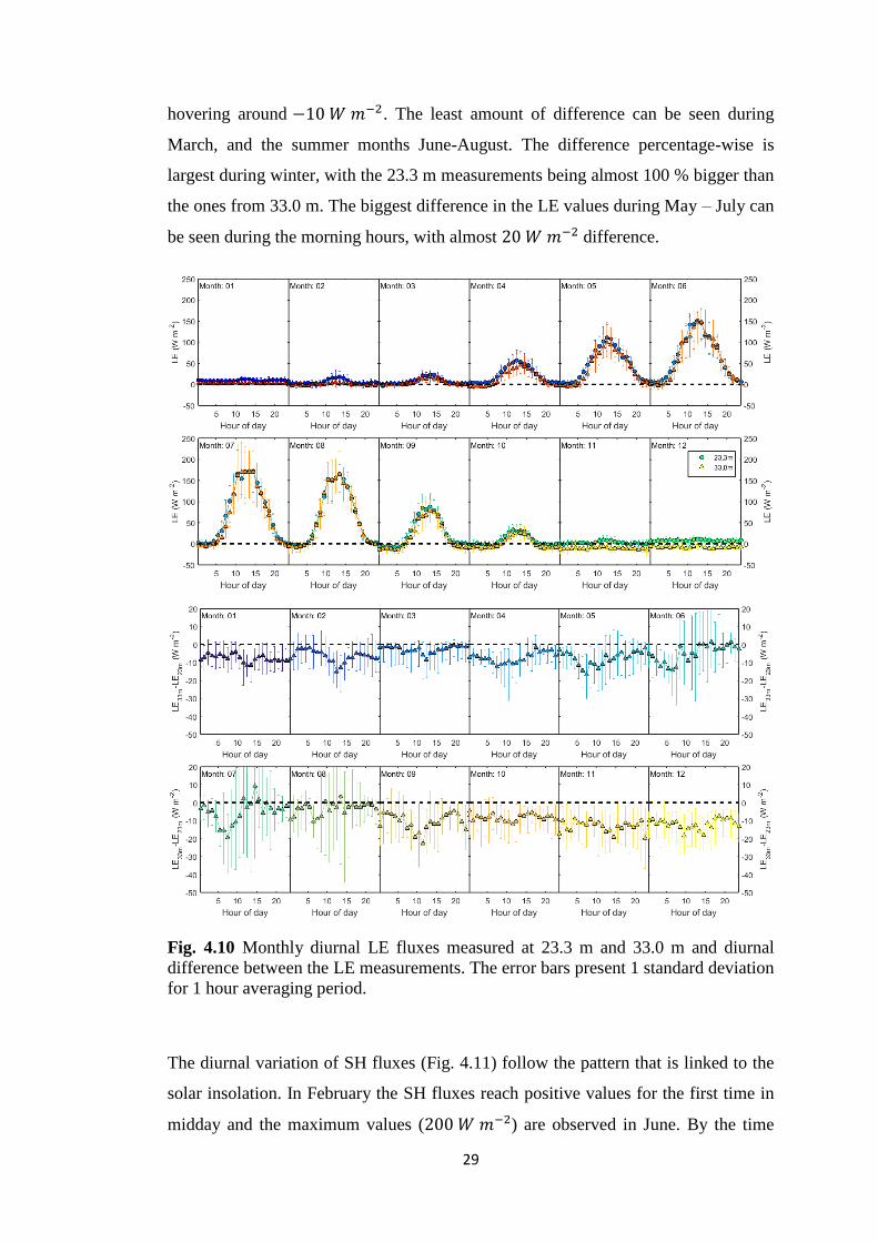
hovering around −10 𝑊 𝑚−2. The least amount of difference can be seen during

March, and the summer months June-August. The difference percentage-wise is

largest during winter, with the 23.3 m measurements being almost 100 % bigger than

the ones from 33.0 m. The biggest difference in the LE values during May – July can

be seen during the morning hours, with almost 20 𝑊 𝑚−2 difference.

Fig. 4.10 Monthly diurnal LE fluxes measured at 23.3 m and 33.0 m and diurnal

difference between the LE measurements. The error bars present 1 standard deviation

for 1 hour averaging period.

The diurnal variation of SH fluxes (Fig. 4.11) follow the pattern that is linked to the

solar insolation. In February the SH fluxes reach positive values for the first time in

midday and the maximum values (200 𝑊 𝑚−2) are observed in June. By the time

30

winter is coming, the sensible heat fluxes have already been decreasing and,

eventually in November, they remain negative during the whole day. The nighttime

values remain almost constant through the year (−20 𝑊 𝑚−2), as they are mainly

dependent on the difference between air and surface temperatures, and also on leaf

area and snow cover. The difference between the measurement set-ups is negligible,

remaining under 20 𝑊 𝑚−2 throughout the year. The difference fluctuates between

positive and negative values, which indicates that there are no consistent differences

between the measurement set-ups.

Fig. 4.11 Monthly diurnal SH fluxes measured at 23.3 m and 33.0 m and diurnal

difference between the SH measurements. The error bars present 1 standard

deviation for 1 hour averaging period.

31

Fig. 4.12 Monthly diurnal friction velocities measured at 23.3 m and 33.0 m and

diurnal difference between the 𝑢∗ measurements. The error bars present 1 standard

deviation for 1 hour averaging period.

The diurnal variation of friction velocities (Fig. 4.12) is largest during the summer,

as there is more variability in turbulence conditions. The friction velocities do not

vary significantly between daytime and nighttime during the winter, but a distinct

diurnal variation can be seen in March-October. In the diurnal cycle the friction

velocity has a minimum during the night and reaches a maximum in midday. The

values measured at 23.3 m are generally speaking slightly greater than those of 33.0

m set-up. However, the difference is quite small, 0.02 𝑚 𝑠−1 ~5 %, proving that

both measurement set-ups operate in similar flow conditions.

32

4.3 Differences due to wind direction

Differences in flux measurements can be caused by the heterogeneities in the

underlying surface. The effect of some topographical or vegetation dependent

differences can be examined through wind direction based observations. Slight

variation of vertical flow between the multiple wind directions is natural due to

weather patterns.

Disturbed wind direction caused by the position of the measurement instruments on

the side of the measurement tower can be seen between 130° and 220° (Fig. 4.13).

However, the distortion does not seem to affect the flux values, as seen with NEE in

Fig. 4.14. Similar results with LE and SH fluxes were obtained with no real

correlation between them and the wind direction (not shown).

Fig. 4.13 Friction velocity difference in all wind directions over the whole year with

bin averages.

33

Fig. 4.14 NEE difference in all wind directions over the whole year with bin

averages.

4.4 Differences due to atmospheric stability

The stability conditions affect the measurements by implying the amount of mixing

occurring in the lower atmosphere. As the measurements are acquired on two

different elevation levels above the ground, the effect of turbulence might vary

between them. Stability does also affect the footprint characteristics, which is

discussed in Sect. 4.5.

The net ecosystem exchange difference between the two measurement set-ups related

to the various stability conditions is shown in figure 4.15. For stable conditions NEE

values at 33.0 m are larger than those of 23.3 m. For unstable conditions NEE values

at 23.3 m are less negative than the measurements acquired at 33.0 m. If we assume

that most stable (unstable) conditions happen during nighttime (daytime), we can

derive that absolute values of 33.0 m NEE are larger on the majority of stability

conditions.

The mean differences seen in figure 4.15 hover around 1 𝜇𝑚𝑜𝑙 𝑚−2𝑠−1, while the

monthly NEE means varies from the winter values of 0.5 𝜇𝑚𝑜𝑙 𝑚−2𝑠−1 to

34

midsummer values of −6 𝜇𝑚𝑜𝑙 𝑚−2𝑠−1 (Fig. 4.1). The difference is the smallest

during the more neutral conditions, although the variation throughout the stability

spectrum is quite constant.

The latent heat values for the 23.3 m set-up are larger than those of the 33.0 m set-up

during all stability conditions, which can be seen from figure 4.16. The difference

between the set-ups is close to zero during the most stable and most unstable

conditions, but grows towards the more neutral atmospheric conditions. The

maximum averaged difference is about 10 𝑊 𝑚−2 on both instances.

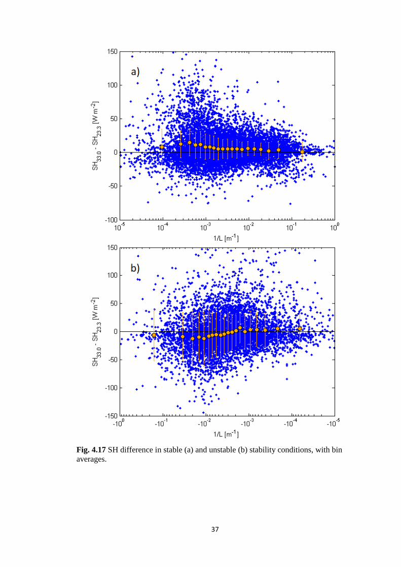
The sensible heat flux difference shown in Fig. 4.17 reveals that both of the

measurement set-ups are recording quite similar values during all stability

conditions. The SH fluxes are observed to be larger for the 33.0 m set-up during

stable conditions and for the 23.3 m set-up during unstable conditions. The

difference in both cases is about 10 𝑊 𝑚−2 and the amount of scatter increases

towards the more neutral conditions.

35

Fig. 4.15 NEE difference in both stable (a) and unstable (b) stability conditions, with

bin averages.

36

Fig. 4.16 LE difference in all stable (a) and unstable (b) stability conditions, with bin

averages.

37

Fig. 4.17 SH difference in stable (a) and unstable (b) stability conditions, with bin

averages.

38

4.5 Footprint analysis

The objective of this analysis is to determine if any differences between the two

measurement set-ups is caused by the meteorological or biological phenomena. The

footprint analysis tackles both aspects when the vegetation distribution is taken into

account. The SMEAR II research station consists mostly of Scots pine (see Sect. 3.1),

but a noticeable patch of spruce trees is located south (135° – 210°) of the

measurement tower. The closest edge of the spruce patch is located at a distance of

180 m from the measurement tower. The footprint is dependent on the measurement

height; the footprint covers larger area when the measurement point is higher. This

notion means that the 33.0 m measurement set-up should get more of its flux signal

from further away than the 23.3 m measurement set-up, and therefore the amount of

difference in flux behavior due to the tree type change at the distance of 180 m can

be observed through the footprint analysis.

In the analysis 21 stability scenarios is picked from the stability distribution to

represent the common stability conditions observed at the site. The distribution of

stability scenarios is shown in Fig. 4.18. Majority of the unstable scenarios fit

between values −10−1.5 < 1 𝐿⁄ < −10−3 , while most of the stable scenarios lie

between 10−3.5 < 1 𝐿⁄ < 10−2. The distribution is limited to consider only the south

direction at which the spruce patch is located. The data also only includes values that

are observed during daytime solar angle of > 10° and nighttime solar angle of < -3°

to avoid intermediate conditions. Üllar Rannik implemented a Lagrangian stochastic

model on these 10 unstable and 11 stable conditions to simulate the footprint

scenarios. The footprint modelling used an approach presented by Rannik et al.

(2003) that was applied to ABL and took into consideration the turbulent dispersion

within the canopy. The footprint scenarios are analyzed at the 90 % cumulative

contribution level and at the distance of 180 m.

39

Fig. 4.18 The amount of unstable (a) and stable (b) half hour runs recorded at 23.3 m,

the 33.0 m set-up has a similar distribution.

In Fig. 4.19 the footprint difference is clearly visible between the two measurement

heights. The unstable values form a tighter spread with higher cumulative footprint

values, while the stable cumulative footprint values grow slower with the distance.

This behavior is fully expected, as discussed in Sect. 2.4. The distance from the

measurement tower is normalized with the tree height 18 m in the Fig. 4.19. The 21

different stability scenarios are representing the distribution of meteorological

conditions observed at the measurement site. The unstable scenarios were modelled

with the source height being 3

4 of the canopy height, while the stable scenarios had

source height set on the ground level.

40

Fig. 4.19 Cumulative flux footprints for 23.3 m (a) and 33.0 m (b). The distance

from the measurement tower and the stability parameter (Obukhov length 𝐿) are

normalized with the canopy height (𝐻 = 18𝑚). Negative 𝐿 𝐻 values correspond to

unstable scenarios and positive 𝐿 𝐻 values to stable scenarios. The distance at which

the pine forest changes into spruce forest in the south is indicated in the figures

(𝑥 𝐻⁄ =180𝑚

18𝑚= 10).

41

In table 4.2 the Fig. 4.19 is further analyzed, with the notion that friction velocity

filtering (Sect. 3.3.1) is done with 𝑢∗ < 0.3 𝑚 𝑠−1, thus excluding some of the most

stable scenarios. The contribution difference varies from 0.3 p.p. to 27.2 p.p. for the

most unstable and fairly stable scenarios, respectively. For slightly stable conditions

the difference of contribution to 90 % cumulative footprint between the two

measurement heights is around 25 p.p. At 90 % cumulative footprint level, during

unstable and neutral conditions, the 23.3 m set-up acquires 80 % or more of its flux

from the pine forest in the south direction, while the 33.0 m set-up acquires only 56 %

or more of its flux from the studied pine forest sector.

Table 4.2 The effect of stability variation to the contribution of pine forest to 90 %

cumulative footprint in south, where the vegetation changes into spruce forest at a

distance of 180 m from the measurement tower. Four of the most stable scenarios are

filtered out of the data in post-processing.

Obukhov

length

1/L [1/m]

Cumulative

footprint

percentage at

180 m distance

[%] 23.3 m

Contribution

of pine forest

to 90 %

cumulative

footprint [%]

23.3 m

Cumulative

footprint

percentage at

180 m distance

[%] 33.0 m

Contribution

of pine forest

to 90 %

cumulative

footprint [%]

33.0 m

Contribution

difference

23.3 m -

33.0 m [p.p.]

Unstable

93.9 100.0 89.75 99.7 0.3

92.2 100.0 87.75 97.5 2.5

88.8 98.7 83.25 92.5 6.2

86.25 95.8 79 87.8 8.1

80.75 89.7 69.75 77.5 12.2

77.5 86.1 63.5 70.6 15.6

74.3 82.6 56 62.2 20.3

73.4 81.6 53.5 59.4 22.1

72.5 80.6 52 57.8 22.8

72 80.0 50.5 56.1 23.9

Stable

56 62.2 32.5 36.1 26.1

55 61.1 31.5 35.0 26.1

52.5 58.3 28.75 31.9 26.4

51 56.7 26.75 29.7 26.9

48 53.3 23.5 26.1 27.2

40 44.4 15.5 17.2 27.2

35 38.9 11 12.2 26.7

26.5 29.4 5 5.6 23.9

22.5 25.0 3 3.3 21.7

17.25 19.2 1 1.1 18.1

13.5 15.0 0.2 0.2 14.8

42

Fig. 4.20 Estimation of the contribution of pine forest to the 90% footprint for

unstable (a) and stable (b) scenarios. Scenarios that are beyond (more stable) the 𝑢∗

filtering, are not used in the flux analysis (see Sect. 3.3.1).

Fig. 4.20 visualizes the contribution of pine forest to 90 % footprint during most of

the atmospheric stability conditions observed at the SMEAR II site. The difference

between the two measurement heights seems to be largest during slightly stable

43

conditions (|1 𝐿⁄ | < 10−3 𝑚−1), and the smallest during most unstable conditions.

The measurement set-ups at 23.3 m and 33.0 m at SMEAR II site are designed to

represent the Scots pine forest, and from Fig. 4.20 the level of representativeness

during various stability conditions can be distinguished. Note that the Scots pine

forest extends further away (a few kilometers) in most of the directions, and that the

footprint analysis considers only the change to spruce forest in the south direction.

4.6 Cumulative ecosystem exchange

The cumulative ecosystem exchange reveal the characteristics of the underlying

ecosystem by for example showing how big of a carbon source or sink it annually is.

It is also a useful way of determining how large the difference between multiple

measurement set-ups is annually.

The cumulative net ecosystem exchange of 23.3 m and 33.0 m set-ups have similar

behavior through the year 2015 (Fig. 4.21). Both of them depict the cumulative

ecosystem respiration during January-March and October-December, when there is

not enough insolation to allow photosynthesis in the boreal vegetation. However a

difference in the amount of respiration can be observed from the figure 4.21 and

based on figure 4.22 it is evident that the 33.0 m measurement set-up is gathering

higher respiration values than the 23.3 m set-up. During the growing season no real

difference in the cumulative NEE values can be observed. The annual cumulative

NEE in units grams of carbon per square meter at the 23.3 m set-up is −294 𝑔𝐶 𝑚−2

and at the 33.0 m set-up −245 𝑔𝐶 𝑚−2, proving that the Scots pine forest acts as a

carbon sink. The cumulative difference between the measurement set-ups is

49 𝑔𝐶 𝑚−2, which is at a satisfying accuracy level ~ 20 % (Baldocchi, 2003). The

result demonstrates that the two measurement set-ups are portraying the same

ecosystem with similar micrometeorological characteristics.

44

Fig. 4.21 Cumulative NEE on the 23.3 m and the 33.0 m set-ups over the year 2015.

Fig. 4.22 Cumulative NEE difference over the year 2015.

45

The ecosystem respiration and uptake were both larger in the 33.0 m measurements

(Fig. 4.2 – 4.3), but they cancel out each other’s effect on NEE during summer,

leaving a small difference between the set-ups. However, in the wintertime, when

there is only ecosystem respiration, the larger values of 33.0 m compared to the ones

from 23.3 m show up in the cumulative NEE.

The annual cumulative LE values are shown in Fig. 4.23 for the 23.3 m measurement

set up and 33.0 m measurement set-up. The results show that the 33.0 m set-up is

collecting lower LE values continuously throughout the year. The annual cumulative

LE for the 23.3 m set-up is 362 𝑚𝑚 and for the 33.0 m set-up 257 𝑚𝑚, while the

difference being 105 𝑚𝑚, meaning that the cumulative value at the 33.0 m is 29 %

smaller.

From figure 4.24 it can be seen that the cumulative difference between the

measurement set-ups grows almost constantly through the whole year, with hardly

any moments where the 33.0 m values are larger than those of 23.3 m.

Fig. 4.23 Cumulative LE on the 23.3 m and the 33.0 m set-ups during the year 2015.

46

Fig. 4.24 Cumulative LE difference during the year 2015.

5. CONCLUSIONS

The aim of this study was to determine the level of uncertainty in forest–atmosphere

exchange while using eddy covariance measurement technique, and to further

determine if the observed deviations could be linked with micrometeorological or

flux footprint related variations or if they were resulted by the uncertainties linked to

the measurement system.

The two measurement set-ups seem to operate in similar micrometeorological setting,

as the differences in friction velocities and wind patterns are small. The proximity of

the canopy top does not have an effect on the lower measurement set-up, even

though it is located only ~ 5 m above the canopy. There are no noticeable differences

in sensible heat measurements between the two heights and they both showcase the

1.5 – 2.0 °C colder average temperatures of June and July (Finnish Meteorological

Institute).

The ecosystem is observed to be a carbon sink as expected, because the pine trees are

still growing. The annual cumulative net ecosystem exchange (NEE) are estimated to

47

be −294 𝑔𝐶 𝑚−2𝑦𝑒𝑎𝑟−1 at the 23.3 m measurement height and

−245 𝑔𝐶 𝑚−2𝑦𝑒𝑎𝑟−1 at the 33.0 m measurement height, respectively. A long-term

ecosystem carbon balance study (Ilvesniemi et al., 2009) conducted at the same

SMEAR II location (23.3 m set-up), showed an average annual NEE of

−206 𝑔𝐶 𝑚−2𝑦𝑒𝑎𝑟−1 during 1995-2008.

The annual cumulative difference of NEE between the two measurement heights is

estimated to be 49 𝑔𝐶 𝑚−2𝑦𝑒𝑎𝑟−1 (~ 17 % difference), which is in the same ballpark

with the total uncertainty of long term EC measurements (±50 𝑔𝐶 𝑚−2𝑦𝑒𝑎𝑟−1) for

measurements at nearly ideal sites (Baldocchi, 2003). A recent study (Rannik et al.,

2006) was conducted in the same measurement station, and showed an estimation of

annual cumulative NEE difference of 80 𝑔𝐶 𝑚−2𝑦𝑒𝑎𝑟−1 between two EC systems

located at the same height (23 m) but with a horizontal separation of 30 m.

The difference in NEE between the two measurement heights can be seen for

example in the monthly diurnal values, where larger ecosystem respiration values are

measured at the 33.0 m set-up during the winter months (November – February). A

model is used to determine the total ecosystem respiration (TER), which has a

greater effect on the NEE percentage-wise more during the winter time.

However, the LE fluxes measured at the two set-ups do not have as strong correlation

with each other as the 𝐶𝑂2 fluxes do. The values of 33.0 m set-up are smaller

throughout the year in all atmospheric conditions, while comparing to the 23.3 m

values. This creates a constant difference to the flux comparison between the

measurement set-ups.

The annual cumulative values of evapotranspiration are 362 mm for the 23.3 m set-

up and 257 mm for the 33.0 m set-up. The annual cumulative evapotranspiration

difference of 105 mm (29 % difference) is much bigger than what is seen with NEE.

The LE measured at 33.0 m behaved peculiarly during November and December

with negative values as if there had been condensation of water vapor at the site.

Even if the cumulative difference might be considered acceptable, the problem is that

the difference does not seem to arise from any specific micrometeorological

phenomena, but could be a measurement system related complication.

The negative LE values that were observed at the 33.0 m measurement set-up may

suggest that condensation of water is occurring at the measurement site. This is

48

unusual especially during winter when the temperatures are below freezing and the

absolute humidity is low. The negative LE values are usually caused by the lack of

sample line heating, enabling condensation inside the sampling tube. When the

unexpected negative LE values were seen while analyzing the measurement data in

autumn of 2016, the heating of the 33.0 m set-up sample line was checked. The

sample line had proper heating then, but from that information no real closure can be

made about the sample line being heated throughout the year 2015.

Another origin for the lower than usual LE values can be dirty interior walls of the

sampling tube, which is affecting the flow through the tube. This dirtiness leads to a

greater attenuation of high frequency fluctuations in water vapor concentrations,

which can be seen in the underestimation of LE (Gholz 2002). However, the

sampling tubes are cleaned regularly and the sampling tube length is only 0.77 m on

the 33.0 m measurement set-up, while it is 7 m on the 23.3 m set-up. The possible

flux attenuation caused by dirty sampling tube would be much greater in the longer

tube, but the results suggest the opposite.

The footprint analysis shows that in south direction (130° – 200°), where the

vegetation changes from pine to spruce, during all atmospheric conditions the 23.3 m

set-ups source area is more often inside the pine forest than with the 33.0 m set-up.

At 90 % cumulative footprint level, during unstable and neutral conditions, the 23.3

m set-up acquires just 80 % of its flux from the pine forest in the south direction,

while the 33.0 m set-up acquires just 56 % of its flux from the same pine forest

sector. However, this difference in vegetation does not seem to affect the annual

carbon budget or the heat fluxes. Neither were there any real correlation found

between wind direction and the 𝐶𝑂2 or energy fluxes.

The measurement height does not seem to influence significantly the flux estimations

made with the eddy covariance method, when the measurement set-ups are located at

the heights of 23.3 m and 33.0 m over the SMEAR II field measurement station.

Exception being the LE flux, but it is not clear how large part of the seen differences

in the results is caused by the measurement height or the measurement system.

49

REFERENCES

Aubinet M et al., 2000. Estimates of the annual net carbon and water exchange of

European forests: the EUROFLUX methodology. Adv. Ecol. Res. 30:113-175.

Aubinet M, Vesala T, Papale D, Eds., 2012. Eddy covariance, a practical guide to

measurement and data analysis. Springer Atmospheric Sciences.

Baldocchi D 2003. Assessing the eddy covariance technique for evaluating carbon

dioxide exchange rates of ecosystems: past, present and future. Glob. Chang. Biol.

9:479-492.

Foken T, 2006. 50 years of the Monin-Obukhov similarity theory. Boundary-Layer

Meteorology 119:431–447.

Foken T, 2008. Micrometeorology. Berlin: Springer.

Gholz H, Clark K, 2002. Energy exchange across a chronosequence of slash pine

forest in Florida. Agr. Forest Meteorol. 112:87-102.

Goulden M et al. 1996. Measurements of carbon sequestration by long-term eddy

covariance: methods and a critical evaluation of accuracy. Glob. Change. Biol.

2:169-182.

Ilvesniemi H et al., 2009. Long-term measurements of the carbon balance of a

boreal Scots pine dominated forest ecosystem. Boreal Environment Research

14:731–753.

Kaimal J, Finnigan J, 1994. Atmospheric boundary layer flows: their structure and

measurement. Oxford: Oxford University Press.

Kolari P et al. 2009. 𝐶𝑂2 exchange and component 𝐶𝑂2 fluxes of a boreal Scots

pine forest. Boreal Environment Research 14:761-783.

Lee X 1998. On micrometeorological observations of surface-air exchange over tall

vegetation. Agr. Forest Meteorol. 91:39-49.

Lofgren B, Zhu Y, 2000. Surface energy fluxes on the Great Lakes based on

satellite-observed surface temperatures 1992 to 1995. J. Great Lakes Res. 26(3):305-

314.

50

Mammarella I et al., 2009. Relative humidity effect on the high frequency

attenuation of water vapour flux measured by a closed path eddy covariance system.

Journal of Atmospheric and Oceanic Technology 26:1856-1866.

Mammarella I et al. 2016. Quantifying the uncertainty of eddy covariance fluxes

due to the use of different software packages and combinations of processing steps in

two contrasting ecosystems. Atmos. Meas. Tech. 9:4915-4933.

Mölder M et al. 2000. Water vapor, 𝐶𝑂2, and temperature profiles in and above a

forest – accuracy assessment of an unattended measurement system. J. Atmos.

Oceanic Technol. 17:417-425.

Oren R et al. 2006. Estimating the uncertainty in annual net ecosystem carbon

exchange: spatial variation in turbulent fluxes and sampling errors in eddy-

covariance measurements. Glob. Chang. Biol. 12:883-896.

Papale D et al. 2006. Towards a standardized processing of net ecosystem exchange

measured with eddy covariance technique: algorithms and uncertainty estimation.

Biogeosciences 3:571-583.

Rannik Ü et al., 2003. Turbulence statistics inside and over forest: influence on

footprint prediction. Bound Layer Meteorol 109:163–189.

Rannik Ü et al. 2004. Estimation of forest-atmosphere 𝐶𝑂2 exchange by eddy

covariance and profile techniques. Agr. Forest Meteorol. 126:141-155.

Rannik Ü et al., 2006. Uncertainties in measurement and modelling of net

ecosystem exchange of a forest. Agr. Forest Meteorol. 138:244-257.

Schmid H et al. 2003. Ecosystem-atmosphere exchange of carbon dioxide over a

mixed hardwood forest in Northern Lower Michigan. J. Geophys. Res. Atmos.

108(D14): Art. No. 4417.

Wesely M, Hart R, 1985. Variability of short term eddy correlation estimates of

mass exchange. In: Hutchinson B, Hicks B (eds) The forest-atmosphere interaction.

D. Reidel, Dordrecht, pp 591-612.

Wilson J, Swaters G, 1991. The source area influencing a measurement in the

planetary boundary-layer – the footprint and the distribution of contact distance.

Bound Layer Meteorol 55:25-46.