uncertainty analysis on … analysis on photogrammetry-derived national shoreline by fang yao b.s....
TRANSCRIPT

UNCERTAINTY ANALYSIS ON PHOTOGRAMMETRY-
DERIVED NATIONAL SHORELINE
BY
FANG YAO
B.S. in Remote Sensing Science and Technology, Wuhan University, 2005
M.S. in Photogrammetry and Remote Sensing, Wuhan University, 2009
THESIS
Submitted to the University of New Hampshire
In Partial Fulfillment of
the Requirements for the Degree of
Master of Science
in
Earth Science
Ocean Mapping
May, 2014

This thesis has been examined and approved.
_______________________________________________
Thesis Director, Dr. Christopher Parrish
Affiliate Professor, UNH
_______________________________________________
Dr. Brian Calder
Associate Director, Center for Coastal and Ocean Mapping
Research Associate Professor, UNH
_______________________________________________
Dr. Shachak Pe’eri
Research Associate Professor, UNH
_______________________________________________
Dr. Yuri Rzhanov
Research Professor, UNH
____________________________________
Date

iii
ACKNOWLEDEGEMENTS
I would like to thank all those people who made this thesis possible.
My first debt of sincere gratitude must go to my advisor, Dr. Christopher Parrish. Given
that my previous research background matched his research direction, he accepted me to
be his student in the Center for Coastal and Ocean Mapping. For this thesis, he offered his
unreserved help and guidance and assisted me with the entire process, from defining the
goals and scope of the research to formatting the thesis. I could not have imagined having
a better advisor and mentor for my graduate study.
Besides my advisor, I would like to thank the rest of thesis committee: Dr. Brian Calder,
Dr. Shachak Pe’eri and Dr. Yuri Rzhanov. They provided valuable and constructive
advices to improve my research and thesis. Considering that English is not my first
language, they also took efforts to correct my endless writing mistakes. I could not have
finished my research and thesis so soon without their encouragement and assistance.
I also thank Center for Coastal and Ocean Mapping. Here I learned a lot of advanced
knowledge and technologies. In addition, it provided the funding which allowed me to
undertake this research and the opportunity to attend conferences to present my research to
others.
Last but not the least, I would like to thank my family: my parents Weixing Yao and
Yunhua Tian, my husband Han Hu, and Han’s parents Boming Hu and Guilan Yao. They

iv
give me a very carefree environment and unconditional love, so that I can concentrate on
my study. I own them too much and wish they could know how much I love and appreciate
them. Thanks.

v
TABLE OF CONTENTS
ACKNOWLEDEGEMENTS ............................................................................................ iii
LIST OF TABLES ............................................................................................................. ix
LIST OF FIGURES ............................................................................................................ x
ABSTRACT ..................................................................................................................... xiii
CHAPTER PAGE
CHAPTER 1 - INTRODUCTION ...................................................................................... 1
1.1 Overview of Shoreline .............................................................................................. 2
1.1.1 Definition of Shoreline ...................................................................................... 2
1.1.2 Importance of Shoreline ..................................................................................... 3
1.2 Photogrammetric Method for Shoreline Mapping .................................................... 4
1.2.1 Shoreline Mapping based on Tide-Coordinated Imagery .................................. 6
1.2.2 Shoreline Mapping based on Non-Tide-Coordinated Imagery ........................ 10
1.3 Overview of Uncertainty Modeling ........................................................................ 12
1.3.1 Systematic and Random Uncertainty ............................................................... 13
1.3.2 Uncertainty Analysis Methods ......................................................................... 13

vi
1.3.2.1 Analytical Method .................................................................................... 13
1.3.2.2 Monte Carlo Method ................................................................................. 15
1.4 Previous Studies for Shoreline Uncertainty Analysis ............................................. 16
1.4.1 Field-Survey-Based Method for Photogrammetry-Derived Shoreline
Uncertainty ................................................................................................................ 16
1.4.2 Empirical Method for LiDAR-Derived Shoreline Uncertainty ....................... 17
1.4.3 Monte Carlo Simulation Method for LiDAR-Derived Shoreline Uncertainty 18
1.5 Research Goals ....................................................................................................... 19
1.6 Thesis Outline ......................................................................................................... 19
CHAPTER 2 - STUDY SITE AND STUDY DATA ....................................................... 21
2.1 Study Site ................................................................................................................ 21
2.2 Study Data ............................................................................................................... 23
2.2.1 Aerial Imagery ................................................................................................. 23
2.2.2 Water Level Data ............................................................................................. 24
2.2.3 Compiled Shorelines ........................................................................................ 26
2.2.4 LiDAR Data ..................................................................................................... 29
CHAPTER 3 - PHOTOGRAMMETRY-DERIVED SHORELINE UNCERTAINTY
ANALYSIS ....................................................................................................................... 31
3.1 Shoreline Uncertainty based on Tide-Coordinated Imagery .................................. 31
3.1.1 Exterior Orientation Element Uncertainty ....................................................... 31

vii
3.1.2 Offset between MHW or MLLW Datum and Observed Water Level ............. 38
3.1.3 Uncertainty in Water Level Data ..................................................................... 40
3.1.4 Human Compilation Uncertainty ..................................................................... 48
3.1.5 Total Propagated Uncertainty .......................................................................... 51
3.2 Shoreline Uncertainty based on Non-Tide-Coordinated Imagery .......................... 55
3.2.1 Exterior Orientation Element Uncertainty ....................................................... 55
3.2.2 Uncertainty in Water Level Data ..................................................................... 55
3.2.3 Human Compilation Uncertainty ..................................................................... 55
3.2.4 Total Propagated Uncertainty .......................................................................... 56
CHAPTER 4 – EXPERIMENTAL RESULT................................................................... 58
4.1 Shoreline Uncertainty based on Tide-Coordinated Imagery .................................. 58
4.1.1 Exterior Orientation Element Uncertainty ....................................................... 58
4.1.2 Offset between MLLW Datum and Observed Water Level ............................ 66
4.1.3 Uncertainty in Water Level Data ..................................................................... 66
4.1.4 Human Compilation Uncertainty ..................................................................... 68
4.1.5 Total Propagated Uncertainty .......................................................................... 69
4.2 Shoreline Uncertainty based on Non-Tide-Coordinated Imagery .......................... 71
4.2.1 Exterior Orientation Element Uncertainty ....................................................... 71
4.2.2 Uncertainty in Water Level Data ..................................................................... 71
4.2.3 Human Compilation Uncertainty ..................................................................... 71

viii
4.2.4 Total Propagated Uncertainty .......................................................................... 73
CHAPTER 5 – DISCUSSION .......................................................................................... 76
5.1 Exterior Orientation Element Uncertainty .............................................................. 76
5.2 Tidal Zoning Uncertainty ........................................................................................ 77
5.3 Human Compilation Uncertainty ............................................................................ 77
5.4 Comparison of Tide-Coordinated and Non-Tide-Coordinated Uncertainties ........ 78
5.5 Relationship between Uncertainty and Slope ......................................................... 79
CHAPTER 6 – CONCLUSIONS AND RECOMMENDATIONS FOR FUTURE WORK
........................................................................................................................................... 82
LIST OF REFERENCES .................................................................................................. 85
APPENDIX: TIDE ANALYSIS REPORT FOR ME1001 ............................................... 92

ix
LIST OF TABLES
Table 2.1 Image acquisition parameters ........................................................................... 24
Table 2.2 Tide Analysis Report (provided by NGS) ........................................................ 25
Table 2.3 Compilation result analysis for 2003 Fort Desoto, Florida project .................. 27
Table 3.1 Uncertainty components for tide-coordinated shoreline ................................... 53
Table 3.2 Uncertainty components for non-tide-coordinated shoreline ........................... 56
Table 4.1 The uncertainty of the ground coordinates caused by the exterior orientation
element uncertainties ........................................................................................................ 61
Table 4.2 The exterior orientation elements of the first image pair .................................. 62
Table 4.3 The exterior orientation elements of the simulated image pair ........................ 64
Table 4.4 Tidal zoning uncertainty analysis for Coffins Point ......................................... 67
Table 4.5 Tide-coordinated human compilation uncertainty computation ....................... 68
Table 5.1 The planimetric values (in meters) of each uncertainty component and the total
uncertainties for the survey area ....................................................................................... 79

x
LIST OF FIGURES
Figure 1.1 Marine boundaries defined by shorelines .......................................................... 3
Figure 1.2 Shoreline mapping, using a plane table and an alidade ..................................... 5
Figure 1.3 MLLW tide windows ........................................................................................ 7
Figure 1.4 A digital photogrammetric system .................................................................... 8
Figure 1.5 Tide-coordinated imagery ................................................................................. 9
Figure 1.6 Non-tide-coordinated imagery ......................................................................... 11
Figure 1.7 Cross section drawing which shows the relationship between MHW datum and
observed water level ......................................................................................................... 12
Figure 1.8 Field-survey-based method for assessing the photogrammetry-derived shoreline
uncertainty......................................................................................................................... 17
Figure 2.1 The survey area for ME1001 ........................................................................... 21
Figure 2.2 The tides at Cobscook Bay .............................................................................. 22
Figure 2.3 The mosaic natural color imagery overlaid on NOAA Chart .......................... 23
Figure 2.4 The mosaic near infrared imagery ................................................................... 24
Figure 2.5 MHW and MLLW lines for the survey area ................................................... 26
Figure 2.6 Two selected areas for non-tide-coordinated human compilation uncertainty
analysis (red boxes) ........................................................................................................... 28
Figure 2.7 Compiled MHW lines from 9 compilers ......................................................... 29
Figure 2.8 LiDAR data for the ME1001 survey area........................................................ 30
xi
Figure 3.1 Space intersection ............................................................................................ 34
Figure 3.2 Configuration of the Monte Carlo analysis method for determining positioning
uncertainty caused by exterior orientation element uncertainty for each image pair ....... 38
Figure 3.3 Offset between the observed water level and MLLW datum at the time the image
was taken ........................................................................................................................... 39
Figure 3.4 An example of Pydro-generated water level relative to MHW and MLLW at the
time of acquisition of each image ..................................................................................... 40
Figure 3.5 TCARI water level uncertainty ....................................................................... 41
Figure 3.6 The tide gauge design used to reduce the current-induced uncertainty ........... 43
Figure 3.7 Human compilation uncertainty analysis ........................................................ 50
Figure 3.8 Flowchart of human compilation uncertainty computation ............................. 51
Figure 4.1 The relationships between the number of the simulation trials and X/Y/Z
uncertainty caused by exterior orientation element uncertainties ..................................... 60
Figure 4.2 The influence of the exterior orientation element uncertainties and the
photographic scale on the point positioning uncertainty (for the first image pair) ........... 64
Figure 4.3 The influence of the exterior orientation element uncertainties and the
photographic scale on the point positioning uncertainty (for the simulated image pair) .. 65
Figure 4.4 Filtered slope raster imagery ........................................................................... 70
Figure 4.5 The reference shorelines (red lines) and transects (blue lines) ........................ 72
Figure 4.6 The relationship between the slope and the planimetric human compilation
uncertainty......................................................................................................................... 73

xii
Figure 4.7 The uncertainty boundaries ............................................................................ 74
Figure 5.1 Distribution of standard uncertainties for tide-coordinated and non-tide-
coordinated compilation .................................................................................................... 80
Figure 5.2 Distribution of slopes ...................................................................................... 81

xiii
ABSTRACT
UNCERTAINTY ANALYSIS ON PHOTOGRAMMETRY-DERIVED
NATIONAL SHORELINE
by
Fang Yao
University of New Hampshire, May, 2014
Photogrammetric shoreline mapping remains the primary method for mapping the national
shoreline used by the National Geodetic Survey (NGS) in the National Oceanic and
Atmospheric Administration (NOAA). To date, NGS has not conducted a statistical
analysis on the photogrammetry-derived shoreline uncertainty. The aim of this thesis is to
develop and test a rigorous total propagated uncertainty (TPU) model for shoreline
compiled from both tide-coordinated and non-tide-coordinated aerial imagery using
photogrammetric methods. Survey imagery collected over a study site in northeast Maine
was used to test the TPU model. The TPU model developed in this thesis can easily be
extended to other areas and may facilitate estimation of uncertainty in inundation models
and marsh migration models.

1
CHAPTER 1 - INTRODUCTION
National shoreline products should be accompanied by uncertainty estimates. These
uncertainties enable users to evaluate the suitability of the national shoreline for other
applications, such as coastal change analysis, and assist in making policy decisions in
coastal zone management. Photogrammetric stereo compilation has been the main method
for shoreline mapping used by the National Geodetic Survey (NGS) since 1927, but
statistical uncertainty analysis has lagged behind other areas of technology development in
photogrammetric shoreline compilation. The only uncertainty estimation method for the
phtogrammetry-derived shoreline that has been well tested and documented to date is a
field survey technique based on high-precision Global Positioning System (GPS), which is
time consuming and economically expensive. In addition, the fieldwork is difficult to
conduct in all shoreline survey regions. Therefore, a statistical model for photogrammetry-
derived uncertainty analysis is needed, which not only satisfies international hydrographic
surveying standards, but can also provide sensitivity analysis for each uncertainty influence
factor.

2
1.1 Overview of Shoreline
1.1.1 Definition of Shoreline
In many publications, a shoreline is succinctly defined as the line where the water and land
meet. However, due to the influence of some factors, such as wave swash, tides, currents,
storms, seasonal beach changes, sediment transportation, natural and human-induced sea-
level changes, the line of intersection between water and land changes continuously
(Graham et al., 2003; Parrish, 2012). Therefore, this succinct definition is not useful in
practice (e.g., in mapping applications and coastal change analysis), as it is not meaningful
to compare intersection lines from different times that depend on the tidal cycle.
In order to circumvent the above problem, many shoreline indicators have been used in
shoreline mapping and described in many publications. However, it is difficult for the
practitioners to agree on a common shoreline indicator. All indicators can be divided into
two categories: (1) physical shoreline indicators (Stokdon et al., 2002; Boak and Turner,
2005), including berm crest, scarp edge, vegetation line, dune toe, dune crest, and cliff or
bluff crest and toe; and (2) water-level based shoreline indicators (Shalowitz, 1964; Pajak
and Leatherman, 2000), including the high water line, mean high water (MHW) line, mean
lower low water (MLLW) line, wet/dry boundary, wet sand line, and water line, etc.
Currently, NGS, the part of the National Oceanic and Atmospheric Administration
(NOAA), which is responsible for mapping the national shoreline depicted on NOAA
nautical charts, compiles the MHW line and MLLW line as shoreline indicators in order to
minimize the tidal daily, monthly and yearly variations (Office of Coast Survey, 2013a).
MHW is the average of all the high water heights observed over the National Tidal Datum

3
Epoch (NTDE), a specific 19-year period which contains all the tidal periods that need to
be considered in tidal computations, whereas MLLW is the average of all the lower low
water heights observed over the NTDE. MHW and MLLW lines are typically marked on
United States (U.S.) NOAA nautical charts. MHW lines are the legal lines of the U.S. and
the boundaries between land and sea. MLLW lines help to define America’s territorial
limits, the Exclusive Economic Zone, and the High Seas (Woodlard et al., 2003).
Figure 1.1 Marine boundaries defined by shorelines. (Courtesy of Office of General
Counsel, NOAA, 2014)
1.1.2 Importance of Shoreline
The areas around the shoreline are rich with diverse species, habitat types, nutrients and
natural resources (WRI, 2000). In addition, approximately half of the world’s population
lives within 200 kilometers of the shoreline (Creel, 2003), and, in the U.S., about 53% of
4
the nation’s population lives in the 673 U.S. coastal counties (Crossett et al., 2004).
Currently, sea level is rising at the rate of ~3 mm/year worldwide (Royal Swedish Academy
of Sciences, 2012), and local rates of sea level rise are higher in some regions. Sea-level
rise can lead to a loss of coastal land and wetland species, such as fish, bird, wildlife and
plants. It can also increase the frequency and extent of coastal flooding, as well as the
impact of coastal storms. Therefore, in order to better understand and analyze these impacts
mentioned above, mapping shorelines has become a significant task worldwide.
Furthermore, an accurately mapped shoreline is of extreme importance to nautical charting
agencies/offices, as well as coastal scientists and coastal zone managers. It supports safe
marine navigation, and legal property boundary definition, as well as a wide range of
coastal science and resource management applications (shoreline change, sea-level rise,
inundation modeling, habitat change, wetlands studies, restoration, etc.) (e.g., Boak and
Turner, 2005).
1.2 Photogrammetric Method for Shoreline Mapping
The earliest shoreline survey in the U.S. was conducted by the U.S. Coast Survey in 1834
along the north shore of Great South Bay, Long Island (Wainwright, 1922). The procedures
of the historical shoreline surveys were field based (Graham et al., 2003) (Figure 1.2).

5
Figure 1.2 Shoreline mapping, using a plane table and an alidade (Courtesy of NGS,
2014a)
Shoreline mapping changed from a field survey approach to a remote sensing approach
with the advent of the airplane and aerial camera. In 1919, the U.S. investigated the
feasibility of aerial photography in shoreline mapping over coastal New Jersey. However,
shoreline mapping was still conducted by field surveys until 1927 (Smith, 1981). With the
increase use of aerial photogrammetric methods since 1927, aerial survey has been used
for mapping shorelines to update nautical charts and is still the primary method for
shoreline mapping in NOAA. Compared with field-based shoreline mapping methods,
photogrammetric methods have several benefits, including the ability to map large areas
with greater detail quickly, and to access certain areas where field surveys cannot be
conducted. As aerial imagery evolved from visible panchromatic to multi-spectral bands
that include three bands in the visible range (red-green-blue) and one band in the near-
infrared range, shoreline mapping procedures using photogrammetry became more

6
accurate and robust. Compared with black and white imagery (i.e., a panchromatic band in
the visible range), color imagery better represents the real world, from which operators can
more easily and better identify and interpret features. In the near infrared (NIR) portion of
the electromagnetic spectrum, water absorbs nearly all the light, which makes water appear
very dark, while land (such as sand and vegetation) has a bright reflectance in this spectral
region. The high contrast between land and water makes it easier to interpret and map
shorelines in NIR imagery. The transition from film-based imagery to digital format also
reduces the time needed from acquisition to a shoreline product.
Currently, photogrammetric shoreline mapping is mainly conducted on tide-coordinated
imagery (taken when the vertical difference between water level and MHW or MLLW is
within a defined tolerance) and non-tide-coordinated imagery (taken when the vertical
difference between water level and MHW or MLLW is out of a defined tolerance).
1.2.1 Shoreline Mapping based on Tide-Coordinated Imagery
Tide-coordinated imagery must be acquired when the tide stage is within the defined
tolerance of MHW or MLLW, which is called the tide window (Graham et al., 2003):
𝑇𝑟 = {±0.09, 𝑟 ≤ 1.5𝑚±0.1𝑟, 𝑟 > 1.5𝑚
(1.1)
where 𝑇𝑟 is the tolerance in meters, and r is the tide range. Figure 1.3 shows the MLLW
tide windows from a water level prediction.

7
Figure 1.3 MLLW tide windows
The tide window is the constraint on image acquisition time. NOAA specifies additional
aerial imagery acquisition requirements for shoreline mapping programs in the “Scope of
Work for Shoreline Mapping under the NOAA Coastal Mapping Program” (Leigh et al.,
2012) in order to acquire aerial imagery with good quality, on which ground objects and
shorelines can be identified and extracted easily.
In shoreline mapping programs, kinematic GPS and Inertial Measurement Unit (IMU)
devices are often used to determine positioning and orientation parameters of image
exposure stations. In this case, ground control may not be needed, or, at least, can be greatly
reduced. This is very useful in areas which cover a lot of water or forest, because ground
control points in these areas are difficult to interpret on the imagery.
Feature compilation is performed in a stereo environment of a digital photogrammetric
system (Figure 1.4). BAE's SOCET SET is a photogrammetric software program
commonly used by NGS to map shorelines (Graham et al., 2003). Three-dimensional
coordinates of ground points are estimated by measurements made in stereo image pairs

8
(adjacent but overlapping aerial images). A ray can be constructed from an exposure station
to a ground point, and the three-dimensional coordinates of the ground point are determined
by the intersection of the corresponding rays (Mikhail et al., 2001).
Figure 1.4 A digital photogrammetric system, which consists of a desktop computer with
specified photogrammetric software, a 3D pointing device and a stereo display system
(Courtesy of NOS, 2014)
Ideally, compilers trace the land-water interface as the MHW or MLLW line in NIR tide-
coordinated imagery because of the sharp contrast between land and water in NIR.
However, wave action may hamper the shoreline interpretation given that it may create
swash zones (Graham et al., 2003). In order to minimize the effect of wave action, tide-
coordinated shoreline is usually delineated in the middle of the average run-up and retreat
limits of the waves. In addition, some indicators can be used to assist shoreline
interpretation, such as the tide’s falling or rising, beach features, berms, tone and texture.
Figure 1.5 shows the MHW and MLLW lines interpreted from tide-coordinated imagery.

9
Figure 1.5 Tide-coordinated imagery. (Top) is MHW tide-coordinated imagery, from
which the MHW line (the blue line) is interpreted. (Bottom) is MLLW tide-coordinated
imagery, from which the MLLW line (the orange line) is interpreted.

10
1.2.2 Shoreline Mapping based on Non-Tide-Coordinated Imagery
When the water level is out of the defined tolerance and below the MHW datum, compliers
will delineate the MHW line mainly based on elevation information on non-tide-
coordinated imagery. Natural color imagery is often used as non-tide-coordinated imagery
given that it can provide more indicators to assist in shoreline compilation. The MLLW
line is seldom compiled on non-tide-coordinated imagery. It is not technologically difficult,
but rather there are fewer opportunities to acquire the imagery when water level is below
the MLLW datum (White et al., 2011).
The differences between non-tide-coordinated and tide-coordinated shoreline mapping
mainly include: (1) the time of imagery acquisition: tide-coordinated imagery is taken
within the MHW or MLLW tide window period; non-tide-coordinated imagery is taken
when the water level is below the MHW datum; and (2) the compilation method used in
the shoreline mapping procedure: for tide-coordinated imagery, the land-water interface is
compiled as MHW or MLLW shoreline; for non-tide-coordinated imagery, the MHW
shoreline is compiled based on stereoscopic measurement of an elevation contour. Figure
1.6 shows non-tide-coordinated imagery on which the MHW shoreline (the blue line) has
been compiled. The MHW shoreline is not the intersection between the water and the land
on this imagery.

11
Figure 1.6 Non-tide-coordinated imagery. The blue line is MHW shoreline compiled on
the non-tide-coordinated imagery.
The procedure for shoreline mapping from non-tide-coordinated imagery only describes
the difference from tide-coordinated shoreline mapping as follows:
(1) Acquire imagery when the water level is below the MHW datum based on predicted
water level data.
(2) Obtain the vertical offset between the MHW datum and observed water level based
on observed water level data.
(3) Measure the elevation of the ground just landward of the land-water interface.
(4) Raise the floating mark up by the vertical offset between the MHW datum and
observed water level to contour the MHW shoreline (Figure 1.7). (Note: a floating
mark is a mark used to indicate the three-dimensional location of a point in a stereo
image pair, and it is used by a photogrammetrist in making stereoscopic
measurement (Philpot, 2012)).

12
Figure 1.7 Cross section drawing which shows the relationship between MHW datum and
observed water level
In addition to photogrammetric shoreline mapping methods, several alternative
technologies were investigated by NGS for shoreline mapping. These include: Light
Detection And Ranging (LiDAR) (Stockdon et al., 2002; Wozencraft and Millar, 2005;
Brock and Purkis, 2009; White et al., 2011), satellite imagery (NGS, 2014b),
Interferometric Synthetic Aperture Radar (IFSAR) (NGS, 2014c), Synthetic Aperture
Radar (SAR) (Alfugara et al., 2011), and hyperspectral imagery (Graham et al., 2003). In
this thesis, the research will only focus on the photogrammetric shoreline mapping
methods.
1.3 Overview of Uncertainty Modeling
As the International Hydrographic Organization (IHO) Standards for Hydrographic
Surveys (S-44) specifies, the uncertainty should be recorded together with the survey data
and meet the IHO requirements. The required positioning uncertainty of the coastline (or
shoreline) at the 95% confidence level is defined to be 10 m for special order and 20 m for
order 1a, 1b and 2 (IHO, 2008).

13
1.3.1 Systematic and Random Uncertainty
Measurement uncertainties can be divided into two basic types: systematic uncertainty and
random uncertainty. Systematic uncertainty is a consistent difference between the
measurements and the actual value of the measured attribute. Random uncertainty is the
uncertainty in measurement which leads to the measurement results being inconsistent
when measuring a constant attribute or quality many times. The cause of systematic
uncertainty can usually be identified, and it can often be estimated and thus eliminated.
The random uncertainty cannot be eliminated. We can only reduce it by averaging a large
number of measurement results under suitable observing conditions (Dieck, 2002).
1.3.2 Uncertainty Analysis Methods
In this study, two uncertainty analysis methods are investigated: analytical methods and
Monte Carlo methods.
1.3.2.1 Analytical Method
If the relationship between a measurand Y and a set of the input quantities {𝑋𝑖 , 1 ≤
𝑖 ≤ 𝑁} is expressed by
𝑌 = 𝑓(𝑋1, 𝑋2, …𝑋𝑛) (1.2)
then an estimate of the measurand Y, denoted by y, can be obtained by the function f using
the input estimates 𝑥1, 𝑥2, … 𝑥𝑛 for the values of n input quantities 𝑋1, 𝑋2, …𝑋𝑛,
𝑦 = 𝑓(𝑥1, 𝑥2, … 𝑥𝑛) (1.3)
14
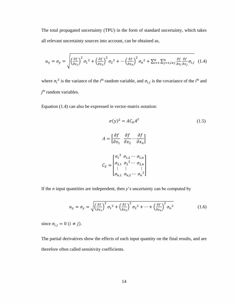
The total propagated uncertainty (TPU) in the form of standard uncertainty, which takes
all relevant uncertainty sources into account, can be obtained as,
𝑢𝑦 = 𝜎𝑦 = √(𝜕𝑓
𝜕𝑥1)2𝜎1
2 + (𝜕𝑓
𝜕𝑥2)2𝜎2
2 + ⋯(𝜕𝑓
𝜕𝑥𝑛)2𝜎𝑛
2 + ∑ ∑𝜕𝑓
𝜕𝑥𝑖
𝜕𝑓
𝜕𝑥𝑗𝜎𝑖,𝑗
𝑛𝑗=1,𝑖≠𝑗
𝑛𝑖=1 (1.4)
where 𝜎𝑖2 is the variance of the ith random variable, and 𝜎𝑖,𝑗 is the covariance of the ith and
jth random variables.
Equation (1.4) can also be expressed in vector-matrix notation:
𝜎(𝑦)2 = 𝐴𝐶𝑋𝐴𝑇 (1.5)
𝐴 = [𝜕𝑓
𝜕𝑥1
𝜕𝑓
𝜕𝑥2⋯
𝜕𝑓
𝜕𝑥𝑛]
𝐶𝑋 =
[ 𝜎1
2 𝜎1,2 ⋯ 𝜎1,𝑛
𝜎2,1 𝜎22 ⋯ 𝜎2,𝑛
⋮ ⋮ ⋮𝜎𝑛,1 𝜎𝑛,2 ⋯ 𝜎𝑛
2]
If the n input quantities are independent, then y’s uncertainty can be computed by
𝑢𝑦 = 𝜎𝑦 = √(𝜕𝑓
𝜕𝑥1)2𝜎1
2 + (𝜕𝑓
𝜕𝑥2)2𝜎2
2 + ⋯+ (𝜕𝑓
𝜕𝑥𝑛)2𝜎𝑛
2 (1.6)
since 𝜎𝑖,𝑗 = 0 (𝑖 ≠ 𝑗).
The partial derivatives show the effects of each input quantity on the final results, and are
therefore often called sensitivity coefficients.

15
The expanded uncertainty, which defines a confidence interval (CI) about the measurement
result within a percentage (%) possibility that the true value of the measurand lies, can be
given by the product of the standard uncertainty and the coverage factor t which depends
on the confidence level and the particular distribution:
𝑈(𝑦) = 𝑡 ∙ 𝑢(𝑦) (1.7)
A 95% confidence level is commonly used in practice, with coverage factor 1.96 for
normally distributed measurement,
𝑈95(𝑦) = 1.96𝑢(𝑦) (1.8)
1.3.2.2 Monte Carlo Method
It is often difficult to use analytical methods to estimate the uncertainty of complex
measurement systems. The Monte Carlo method was devised to solve some difficult
deterministic problems by running random simulations many times to obtain the
distribution of the probabilistic outputs (Papadopoulos and Yeung, 2001). The concept
behind the Monte Carlo method is to generate a large number of experimental trials from
which the distribution function of the output quantity can be estimated. When applied to
uncertainty analysis, one form of the Monte Carlo method is:
(1) A sample of n input quantities {𝑥1, 𝑥2, … 𝑥𝑛} is generated m times based on the
probability density function of each input quantity (or the joint distribution of all
the input quantities, if known).
(2) The output for each set of input quantities can be obtained,
𝑦𝑗 = 𝑓(𝑥1,𝑗 , 𝑥2,𝑗 , … 𝑥𝑛,𝑗) (1.9)

16
for j = 1, 2, …m.
(3) The probability density function of y can be estimated from 𝑦1, 𝑦2 …𝑦𝑚. From this,
the uncertainty of y can be also obtained.
Compared with the analytical method, the Monte Carlo method has some advantages. For
example: (1) it is not necessary to compute complex partial derivatives; (2) it takes care of
the dependencies of input quantities; and (3) it can deal with small and large uncertainties
of input quantities (Papadopoulos and Yeung, 2001). Its biggest drawback is the
computational cost. More realizations in the Monte Carlo simulations will provide a more
accurate solution, but computation time will increase.
1.4 Previous Studies for Shoreline Uncertainty Analysis
To date, NGS does not have a statistical uncertainty model for photogrammetry-derived
shorelines. Instead, field-survey-based methods have been used to evaluate the
photogrammetry-derived shoreline uncertainty. In addition, empirical methods and
stochastic methods are used for LiDAR-derived shoreline uncertainty (White et al., 2011).
1.4.1 Field-Survey-Based Method for Photogrammetry-Derived Shoreline Uncertainty
The field-survey-based method has been used to estimate the uncertainty of
photogrammetry-derived shoreline. Surveyors walk along the interface of land and water
and use GPS to measure the three-dimensional coordinates of the interface points at the
time when aerial images are taken (Figure 1.8). The shoreline generated by connecting
these points is considered as the “true” shoreline and then compared with the

17
photogrammetry-derived shoreline to compute the uncertainty of the photogrammetry-
derived shoreline (Hutchins, 1994).
Figure 1.8 Field-survey-based method for assessing the photogrammetry-derived
shoreline uncertainty
This method has some drawbacks: (1) this field-survey-based method requires a large-scale
deployment, which makes it impractical to conduct this method with each photogrammetric
shoreline project; (2) it cannot provide sensitivity analysis (the influence of different
factors on the final result), and it is not known how to control or decrease the uncertainty;
and (3) the GPS-measured shoreline is not the actual true MHW or MLLW line. The
instantaneous shoreline most likely will not be the same as the MHW or MLLW line due
to some dynamic effects. In addition, GPS measurement still has uncertainty.
1.4.2 Empirical Method for LiDAR-Derived Shoreline Uncertainty
In 2008, NGS used a Topcon Laser-Zone integrated laser level and real-time GPS systems
to assess the uncertainty of the LiDAR-derived shoreline along the North Carolina Outer
Banks (White et al., 2011). The coordinates of points near the shoreline were measured at
a spacing of ~5m along each transect, which was oriented perpendicular to the shoreline.
The spacing between transects was ~10m. The MHW zero-crossing points were

18
interpolated from the measured points. Finally, the spatial (Euclidean) distance from these
MHW zero-crossing points to the points on the LiDAR-derived shoreline vector was
computed to estimate the shoreline uncertainty.
The main benefit of this method is that it is independent of the data, whose uncertainty is
assessed by it. However, this method has also the same drawbacks as the field-survey-
based method for photogrammetry-derived shoreline. Therefore, as the IHO S-44
specifications mandates, a statistical method should be adopted to determine positioning
uncertainty by combining all uncertainty sources (IHO, 2008).
1.4.3 Monte Carlo Simulation Method for LiDAR-Derived Shoreline Uncertainty
A Monte Carlo simulation method for topographic LiDAR-derived shoreline uncertainty
was developed by White et al. (2011). The ranges and angles of the transmitted light pulses
were acquired by back-projecting the laser geolocation equation (Lindenberger, 1989;
Vaughn et al., 1996; Filin, 2001) with the known coordinates of the ground points and the
known positions and orientations of the LiDAR sensor. Based on the uncertainties of
positions, attitudes, ranges and angles, a series of plausible estimates of these variables
were formed. Through the process of normal geolocation, Digital Terrain Model (DTM)
construction and shoreline extraction, a series of shorelines were then extracted to analyze
the shoreline uncertainty.
This simulation method satisfies the IHO S-44 standards, and it is a statistical method,
which does not require expensive field surveys. In addition, it can perform sensitivity
analysis, through which users can know how each factor influences the final shoreline

19
uncertainty. However, this method has not been extended to the photogrammetry-derived
shoreline uncertainty analysis.
1.5 Research Goals
Photogrammetric stereo compilation is the main shoreline mapping method used by NGS.
Based on the review provided above, there is no adopted statistical method to estimate the
photogrammetry-derived shoreline uncertainty. With this as an objective, this research
provides a discussion of uncertainties involved in photogrammetric shoreline mapping and
develops a TPU model in order to: (1) generate accuracy metadata for the national
shoreline; (2) satisfy IHO S-44 Standards for Hydrographic Surveys; (3) help to make
informed policy decisions; and (4) enable computation of uncertainty in shoreline change
rate estimates and other derived data products.
1.6 Thesis Outline
The reminder of this thesis is organized as follows. Chapter 2 describes the study site and
data. Chapter 3 presents the photogrammetry-derived shoreline uncertainty analysis for
two cases: first, where the main uncertainty components for tide-coordinated imagery
include exterior orientation element uncertainty, offset between MHW or MLLW datum
and observed water level, uncertainty in water level data and human compilation
uncertainty; and second, where the main uncertainty components for non-tide-coordinated
imagery include exterior orientation element uncertainty, uncertainty in water level data
and human compilation uncertainty. Chapter 4 discusses experimental results for the study

20
area. Chapter 5 contains an in-depth discussion of the results. Finally, chapter 6 contains
conclusions and recommendations for future work.

21
CHAPTER 2 - STUDY SITE AND STUDY DATA
2.1 Study Site
On June 21st 2011, a NOAA NGS aerial survey (ME1001) was conducted to provide aerial
images of the strait that links Dennys Bay, Whiting Bay and Cobscook Bay in the northeast
coastal region of Maine, and this survey also covered other bays, entrances, and tributaries
to the project area (Figure 2.1).
Figure 2.1 The survey area for ME1001. (Left) The blue area is the state of Maine, and
the red box is the survey area; (right) The imagery of the survey area from ArcGIS
imagery basemap
The region is characterized by a large tide range and strong tidal currents with an average
tide range at Cobscook Bay of 7.3 m (which can exceed 8.5 m during spring tide).

22
Typically, a large volume of sea water flows in and out of it twice daily, which creates
significant currents (NOAA Fisheries, 2014). The current can exceed 1.5 m/s (Xu et al.,
2006). Figure 2.2 shows the high tide and the low tide at Cobscook Bay. The study site
contains numerous embayments (right image in Figure 2.1). The shoreline along the study
site contains a wide range of beach slopes. Based on an analysis using ArcGIS and LiDAR
data download from Digital Coast (Coastal Service Center, 2013), the slope range in the
study site ranges from 1° to 46°, with the average slope being ~14°. The shoreline can be
segmented into different types of convoluted shorelines, ranging from rock outcrops to
gravel pocket beaches and tidal mudflats. The complexity of the site and the range of
shoreline types covered were determined to be advantageous for developing the shoreline
TPU model. In particular, it should be possible to extend the TPU model and procedures
to other project sites that are less complex and exhibit greater homogeneity of shoreline
type, whereas the reverse would not necessarily be true. It is also important to note that,
due to the complexity of the shoreline in this region, the shoreline uncertainty is expected
to generally be higher than that in other areas.
Figure 2.2 The tides at Cobscook Bay. (Left) High tide at 2:25 pm on September 19th,
2012; (right) low tide at 9:36 am on September 20th, 2012 (Courtesy of Kinexxions,
2014)

23
2.2 Study Data
2.2.1 Aerial Imagery
Seventy natural color and NIR images were taken using an Applanix Digital Sensor System
(DSS) 439 DualCam at an altitude of 3048 m along two flight lines 50-001 and 50-002
(each flown twice). The mosaic natural color imagery, the flight lines and the tide gauges
are depicted in Figure 2.3. Figure 2.4 is the mosaic NIR imagery. Table 2.1 provides the
image acquisition parameters. In addition, a custom exterior orientation element report was
output from POSPac (Applanix software for direct georeferencing of airborne imaging
sensors (Applanix, 2013)) containing the exterior orientation elements of each image and
also their standard uncertainties.
Figure 2.3 The mosaic natural color imagery overlaid on NOAA Chart (Office of Coast
Survey, 2013b) (The red lines are the two flight lines. The red stars are the three tide
gauges used in this survey)

24
Figure 2.4 The mosaic near infrared imagery
Table 2.1 Image acquisition parameters
Flying height 3048 m (10000 feet)
Camera focal length 60.265 mm
Pixel size on CCD chip 6.8 m
CCD length in the along-track direction 5408 pixels
CCD length in the across-track direction 7212 pixels
2.2.2 Water Level Data
The tide gauges used for this survey were Coffins Point and Birch Island (both subordinate
stations), and Eastport (19-year control station).
An NGS compiler performed tidal level calculations by applying the tidal correctors (time
difference and range ratio) to Eastport’s observations downloaded from the NOAA
25
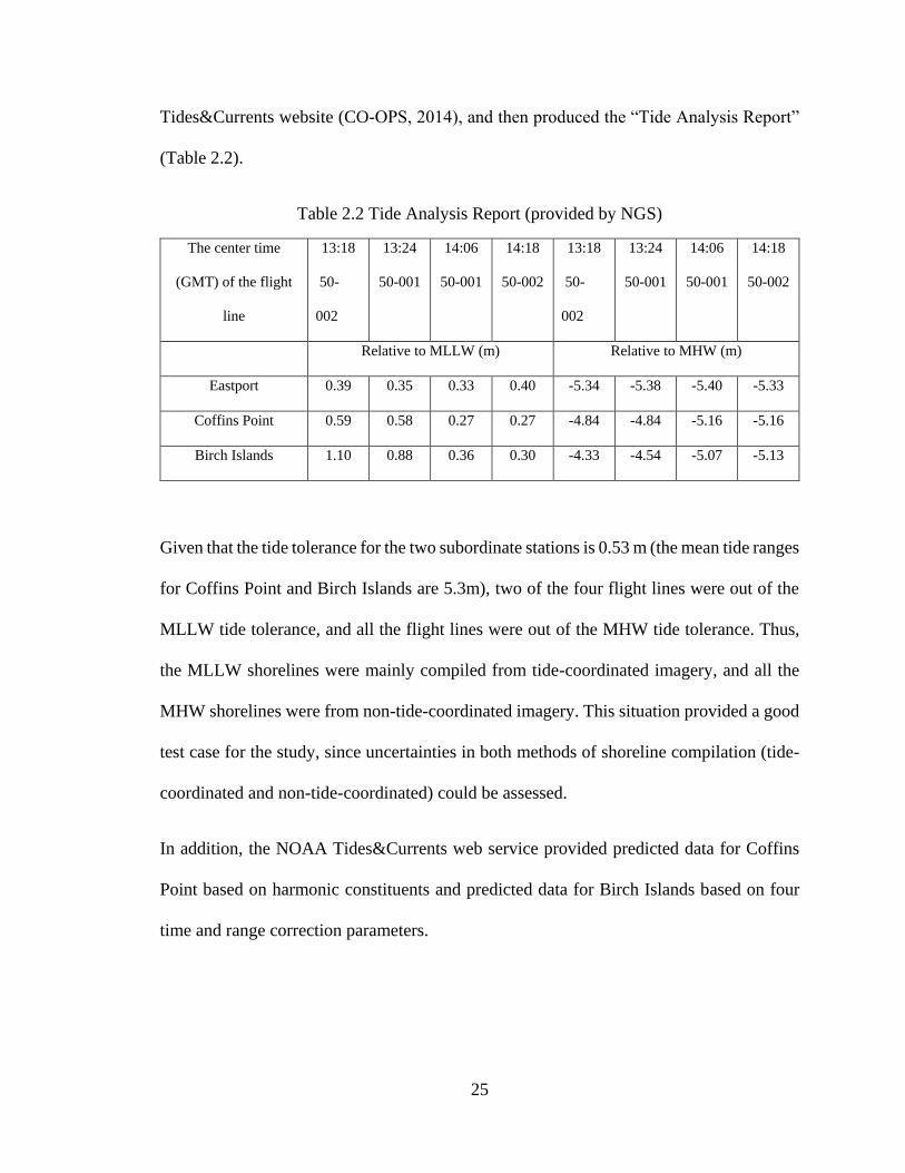
Tides&Currents website (CO-OPS, 2014), and then produced the “Tide Analysis Report”
(Table 2.2).
Table 2.2 Tide Analysis Report (provided by NGS)
The center time
(GMT) of the flight
line
13:18
50-
002
13:24
50-001
14:06
50-001
14:18
50-002
13:18
50-
002
13:24
50-001
14:06
50-001
14:18
50-002
Relative to MLLW (m) Relative to MHW (m)
Eastport 0.39 0.35 0.33 0.40 -5.34 -5.38 -5.40 -5.33
Coffins Point 0.59 0.58 0.27 0.27 -4.84 -4.84 -5.16 -5.16
Birch Islands 1.10 0.88 0.36 0.30 -4.33 -4.54 -5.07 -5.13
Given that the tide tolerance for the two subordinate stations is 0.53 m (the mean tide ranges
for Coffins Point and Birch Islands are 5.3m), two of the four flight lines were out of the
MLLW tide tolerance, and all the flight lines were out of the MHW tide tolerance. Thus,
the MLLW shorelines were mainly compiled from tide-coordinated imagery, and all the
MHW shorelines were from non-tide-coordinated imagery. This situation provided a good
test case for the study, since uncertainties in both methods of shoreline compilation (tide-
coordinated and non-tide-coordinated) could be assessed.
In addition, the NOAA Tides&Currents web service provided predicted data for Coffins
Point based on harmonic constituents and predicted data for Birch Islands based on four
time and range correction parameters.
26
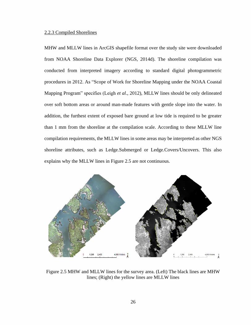
2.2.3 Compiled Shorelines
MHW and MLLW lines in ArcGIS shapefile format over the study site were downloaded
from NOAA Shoreline Data Explorer (NGS, 2014d). The shoreline compilation was
conducted from interpreted imagery according to standard digital photogrammetric
procedures in 2012. As “Scope of Work for Shoreline Mapping under the NOAA Coastal
Mapping Program” specifies (Leigh et al., 2012), MLLW lines should be only delineated
over soft bottom areas or around man-made features with gentle slope into the water. In
addition, the furthest extent of exposed bare ground at low tide is required to be greater
than 1 mm from the shoreline at the compilation scale. According to these MLLW line
compilation requirements, the MLLW lines in some areas may be interpreted as other NGS
shoreline attributes, such as Ledge.Submerged or Ledge.Covers/Uncovers. This also
explains why the MLLW lines in Figure 2.5 are not continuous.
Figure 2.5 MHW and MLLW lines for the survey area. (Left) The black lines are MHW
lines; (Right) the yellow lines are MLLW lines
27
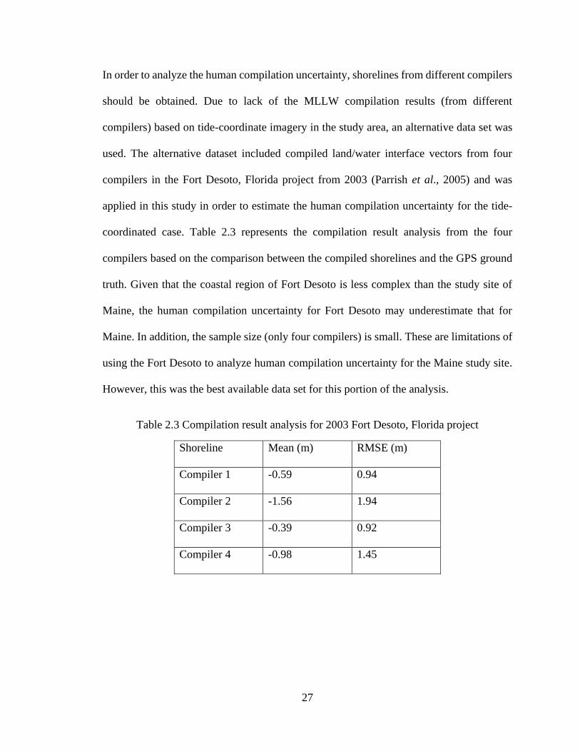
In order to analyze the human compilation uncertainty, shorelines from different compilers
should be obtained. Due to lack of the MLLW compilation results (from different
compilers) based on tide-coordinate imagery in the study area, an alternative data set was
used. The alternative dataset included compiled land/water interface vectors from four
compilers in the Fort Desoto, Florida project from 2003 (Parrish et al., 2005) and was
applied in this study in order to estimate the human compilation uncertainty for the tide-
coordinated case. Table 2.3 represents the compilation result analysis from the four
compilers based on the comparison between the compiled shorelines and the GPS ground
truth. Given that the coastal region of Fort Desoto is less complex than the study site of
Maine, the human compilation uncertainty for Fort Desoto may underestimate that for
Maine. In addition, the sample size (only four compilers) is small. These are limitations of
using the Fort Desoto to analyze human compilation uncertainty for the Maine study site.
However, this was the best available data set for this portion of the analysis.
Table 2.3 Compilation result analysis for 2003 Fort Desoto, Florida project
Shoreline Mean (m) RMSE (m)
Compiler 1 -0.59 0.94
Compiler 2 -1.56 1.94
Compiler 3 -0.39 0.92
Compiler 4 -0.98 1.45

28
For the analysis of the non-tide-coordinated human compilation uncertainty, nine NGS
compilers with different experience levels compiled the MHW lines from non-tide-
coordinated imagery in two selected areas (Figure 2.6and Figure 2.7).
Figure 2.6 Two selected areas for non-tide-coordinated human compilation uncertainty
analysis (red boxes)

29
Figure 2.7 Compiled MHW lines from 9 compilers
2.2.4 LiDAR Data
LiDAR topographic data were collected at a 2 m nominal point spacing for coastal Maine
as part of 2010 U.S. Geological Survey (USGS) American Recovery and Reinvestment
Act (ARRA) LiDAR project, while there was no snow on the ground and water was at or
below normal levels. The vertical accuracy of the data is 0.15 m.

30
The LiDAR data over the study site were downloaded from the Digital Coast web service
(Coastal Services Center, 2013) and were applied to exact the beach slope. This data set is
a raster image file of Z values (GeoTiff format) with a grid cell size of 3 m by 3 m.
Figure 2.8 LiDAR data for the ME1001 survey area

31
CHAPTER 3 - PHOTOGRAMMETRY-DERIVED SHORELINE
UNCERTAINTY ANALYSIS
Although the photogrammetric stereo compilation technology is well understood for terrain
analysis over dry areas away from the coast (McGlone et al. 2004), measurement and
compilation uncertainties are still not adequately modeled in shoreline mapping. This
chapter will discuss the uncertainty components and the total propagated uncertainty model
for tide-coordinated and non-tide-coordinated shoreline mapping. As described in section
3.1, the main uncertainty components for tide-coordinated shoreline mapping include
exterior orientation element uncertainty, offset between MHW or MLLW datum and
observed water level, uncertainty in water level data, and human compilation uncertainty.
As described in section 3.2, the main uncertainty components for non-tide-coordinated
shoreline mapping include exterior orientation element uncertainty, uncertainty in water
level data, and human compilation uncertainty.
3.1 Shoreline Uncertainty based on Tide-Coordinated Imagery
3.1.1 Exterior Orientation Element Uncertainty
In order to derive three-dimensional ground coordinates from two-dimensional image
space, the photogrammetric mapping workflow includes: interior orientation, relative
orientation, absolute orientation, and feature exaction (McGlone et al., 2004). Interior

32
orientation establishes the relationship between the pixel and the image coordinate system.
Relative orientation determines the relative position and orientation of two overlapping
images with respect to one another by measuring some corresponding image points in the
overlapping area of the images. Absolute orientation establishes the relationship between
the image coordinate system and the object space coordinate system by acquiring the
position and attitude of each exposure station which are represented by six exterior
orientation elements: 𝑋𝐿, 𝑌𝐿, 𝑍𝐿, 𝜔, 𝜑, 𝜅. In absolute orientation, ground control points are
generally required. After exterior orientation elements are obtained, ground point
coordinates are acquired by intersecting two corresponding rays from two exposure
stations, and then feature extraction can be implemented. The following collinearity
equations present the relationship among exposure stations, image points and ground
points.
𝑋 − 𝑋𝐿1 = (𝑍 − 𝑍𝐿1)𝑚11,1(𝑥1−𝑥0)+𝑚21,1(𝑦1−𝑦0)+𝑚31,1(−𝑓)
𝑚13,1(𝑥1−𝑥0)+𝑚23,1(𝑦1−𝑦0)+𝑚33,1(−𝑓) (3.1)
𝑌 − 𝑌𝐿1 = (𝑍 − 𝑍𝐿1)𝑚12,1(𝑥1−𝑥0)+𝑚22,1(𝑦1−𝑦0)+𝑚32,1(−𝑓)
𝑚13,1(𝑥1−𝑥0)+𝑚23,1(𝑦1−𝑦0)+𝑚33,1(−𝑓) (3.2)
𝑋 − 𝑋𝐿2 = (𝑍 − 𝑍𝐿2)𝑚11,2(𝑥2−𝑥0)+𝑚21,2(𝑦2−𝑦0)+𝑚31,2(−𝑓)
𝑚13,2(𝑥2−𝑥0)+𝑚23,2(𝑦2−𝑦0)+𝑚33,2(−𝑓) (3.3)
𝑌 − 𝑌𝐿2 = (𝑍 − 𝑍𝐿2)𝑚12,2(𝑥2−𝑥0)+𝑚22,2(𝑦2−𝑦0)+𝑚32,2(−𝑓)
𝑚13,2(𝑥2−𝑥0)+𝑚23,2(𝑦2−𝑦0)+𝑚33,2(−𝑓) (3.4)
𝑀 = [
𝑚11 𝑚12 𝑚13
𝑚21 𝑚22 𝑚23
𝑚31 𝑚32 𝑚33
]
𝑚11 = 𝑐𝑜𝑠 𝜑 𝑐𝑜𝑠 𝜅
𝑚12 = 𝑐𝑜𝑠 𝜔 𝑠𝑖𝑛 𝜅 + 𝑠𝑖𝑛 𝜔 𝑠𝑖𝑛 𝜑 𝑐𝑜𝑠 𝜅

33
𝑚13 = 𝑠𝑖𝑛 𝜔 𝑠𝑖𝑛 𝜅 − 𝑐𝑜𝑠 𝜔 𝑠𝑖𝑛 𝜑 𝑐𝑜𝑠 𝜅
𝑚21 = −𝑐𝑜𝑠 𝜑 𝑠𝑖𝑛 𝜅
𝑚22 = 𝑐𝑜𝑠 𝜔 𝑐𝑜𝑠 𝜅 − 𝑠𝑖𝑛 𝜔 𝑠𝑖𝑛 𝜑 𝑠𝑖𝑛 𝜅
𝑚23 = 𝑠𝑖𝑛 𝜔 𝑐𝑜𝑠 𝜅 + 𝑐𝑜𝑠 𝜔 𝑠𝑖𝑛 𝜑 𝑠𝑖𝑛 𝜅
𝑚31 = 𝑠𝑖𝑛 𝜑
𝑚32 = −𝑠𝑖𝑛 𝜔 𝑐𝑜𝑠 𝜑
𝑚33 = 𝑐𝑜𝑠 𝜔 𝑐𝑜𝑠 𝜑
where (X, Y, Z) are the ground point coordinates, (𝑥1, 𝑦1) and (𝑥2, 𝑦2) are the image space
coordinates of the corresponding image points on image 1 and image 2, f is the focal length,
(𝑋𝐿1, 𝑌𝐿1, 𝑍𝐿1) and (𝑋𝐿2, 𝑌𝐿2, 𝑍𝐿2) are the coordinates of exposure station 1 and exposure
station 2, the rotation matrix M is given by Eq. 4-18b of Mikhail et al. (2001), the elements
of M are the functions of three exterior orientation angle elements (𝜔, 𝜑, 𝜅). (𝑥0, 𝑦0) are
the principal point offsets, and in this thesis we ignore their effect on the positioning
accuracy and set (𝑥0, 𝑦0) = (0, 0). With known exterior orientation elements and measured
corresponding image point coordinates, ground point coordinates can be estimated with the
least square method based on the above four equations (Figure 3.1).

34
Figure 3.1 Space intersection
The use of an integrated GPS/IMU system makes direct georeferencing without ground
control points possible in aerial photogrammetry (Schwarz et al., 1993; Grejner-
Brzezinska, 1999), as the system can provide accurate exterior orientation elements of
exposure stations. Direct georeferencing overcomes some disadvantages of traditional
aerial photogrammetry: complex workflow, inefficiency, and dependence on ground
control points (Maune, 2007; Yuan and Zhang, 2008). With the wide application of direct
georeferencing technology, estimates of the accuracy must be developed in order to (1)
Z
Y
XL1
YL1
ZL1
Y
X
Z
x1 y1
f x
y
O1
L1
XL2
Y
Image coordinate system
Object space coordinate system
1
1
1

35
determine if a given integrated GPS/IMU system can meet the need of the actual
application prior to a survey; (2) provide accuracy metadata for a direct georeferencing
result (White et al., 2011); and (3) enable uncertainty analysis in downstream products
(Parrish, 2011).
The uncertainty components in direct georeferencing mainly include: interior orientation
element (𝑥0, 𝑦0, 𝑓 ) uncertainty, exterior orientation element (𝑋𝐿1 , 𝑌𝐿1 , 𝑍𝐿1 , 𝜔 , 𝜑 , 𝜅 )
uncertainty and uncertainty of corresponding image point coordinate measurement. The
influence of interior orientation element uncertainty on direct georeferencing accuracy is
much smaller than that of exterior orientation element uncertainty, particularly with a well-
calibrated camera (Zhang and Yuan, 2008). This thesis focuses on measurement and
processing uncertainty, which is treated as first-order uncertainty. Calibration uncertainty
is treated as second-order uncertainty and ignored in this thesis. The uncertainty of image
point coordinate measurement can be treated as part of the human compilation uncertainty,
which will be discussed later. Therefore, this section only focuses on exterior orientation
element uncertainty.
Some researchers have analyzed the effect of exterior orientation element uncertainties on
ground point positioning (Zhang and Yuan, 2008; Yuan and Zhang, 2008; Mostafa et al.,
2001). The uncertainty of direct georeferencing based on collinearity equations computed
by error equations (Zhang and Yuan, 2008; Yuan and Zhang, 2008) is actually the least
square estimation uncertainty rather than the positioning uncertainty caused by exterior
orientation element uncertainties. Mostafa et al. (2001) analyzed the positioning accuracy
of some POS/AVTM systems in different photographic scales based on standard error
propagation theory. However, because ground point coordinates are estimated by the least

36
square method, the derivation of error propagation formula is quite complex and is easy to
get wrong. Furthermore, during linearization the nonlinear model errors are introduced due
to not taking some high order terms into account (Papadopoulos and Yeung, 2001).
Therefore, the conventional uncertainty analysis method is not optimal for this problem.
Currently, most relevant research estimates the final ground point positioning accuracy
depending on some measured corresponding image point coordinates. The positioning
accuracy cannot be obtained without corresponding image point coordinate measurements
using these methods. In this thesis, a Monte Carlo simulation method is developed to
estimate the propagated uncertainty in ground point coordinates caused by exterior
orientation element uncertainties, and no measured corresponding image point coordinates
are needed in this method.
For a specific direct georeferencing survey, with the exterior orientation elements and their
uncertainties of each image known, the ground point positioning uncertainty for the whole
survey area can be obtained by computing the root mean square (RMS) of the uncertainties
of all the stereo image pairs. The steps of the uncertainty computation method for each
stereo image pair are as follows:
(1) One hundred equally spaced image points are selected from image 1. For each
image point, the uncertainty computation steps are from (2) to (7).
(2) With the known exterior orientation elements of image 1 (𝑌𝐿1, 𝑍𝐿1, 𝜔1, 𝜑1, 𝜅1), the
image point coordinates (𝑥1, 𝑦1 ) and the average elevation of the survey area,
estimate the corresponding ground point coordinates (X, Y, Z) by the collinearity
equations.
37
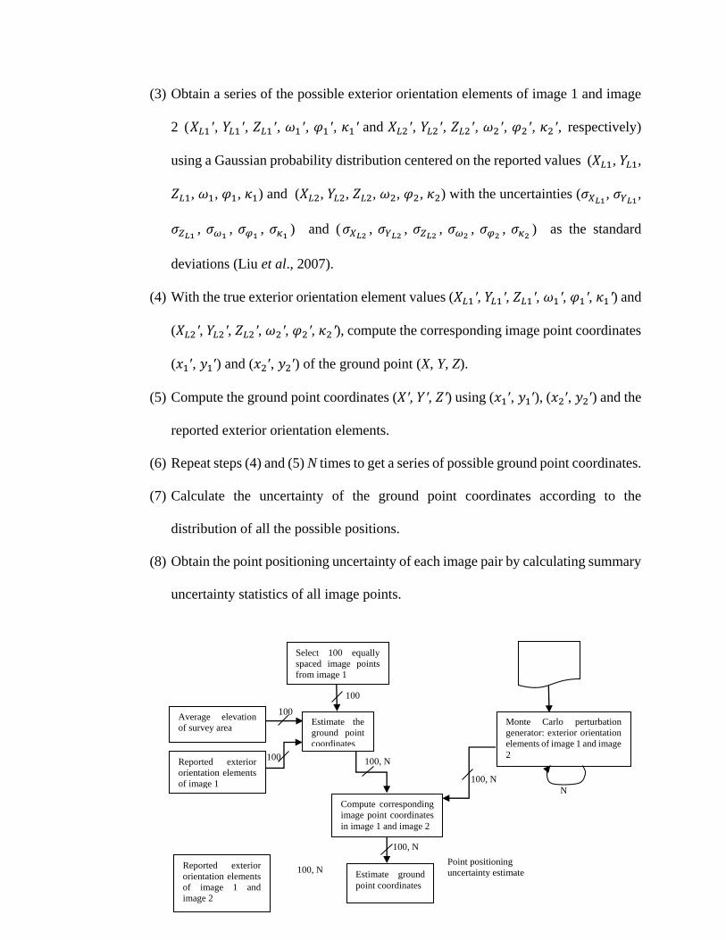
(3) Obtain a series of the possible exterior orientation elements of image 1 and image
2 (𝑋𝐿1′, 𝑌𝐿1′, 𝑍𝐿1′, 𝜔1′, 𝜑1′, 𝜅1′ and 𝑋𝐿2′, 𝑌𝐿2′, 𝑍𝐿2′, 𝜔2′, 𝜑2′, 𝜅2′, respectively)
using a Gaussian probability distribution centered on the reported values (𝑋𝐿1, 𝑌𝐿1,
𝑍𝐿1, 𝜔1, 𝜑1, 𝜅1) and (𝑋𝐿2, 𝑌𝐿2, 𝑍𝐿2, 𝜔2, 𝜑2, 𝜅2) with the uncertainties (𝜎𝑋𝐿1, 𝜎𝑌𝐿1
,
𝜎𝑍𝐿1, 𝜎𝜔1
, 𝜎𝜑1, 𝜎𝜅1
) and (𝜎𝑋𝐿2, 𝜎𝑌𝐿2
, 𝜎𝑍𝐿2, 𝜎𝜔2
, 𝜎𝜑2, 𝜎𝜅2
) as the standard
deviations (Liu et al., 2007).
(4) With the true exterior orientation element values (𝑋𝐿1′, 𝑌𝐿1′, 𝑍𝐿1′, 𝜔1′, 𝜑1′, 𝜅1′) and
(𝑋𝐿2′, 𝑌𝐿2′, 𝑍𝐿2′, 𝜔2′, 𝜑2′, 𝜅2′), compute the corresponding image point coordinates
(𝑥1′, 𝑦1′) and (𝑥2′, 𝑦2′) of the ground point (X, Y, Z).
(5) Compute the ground point coordinates (𝑋′, 𝑌′, 𝑍′) using (𝑥1′, 𝑦1′), (𝑥2′, 𝑦2′) and the
reported exterior orientation elements.
(6) Repeat steps (4) and (5) N times to get a series of possible ground point coordinates.
(7) Calculate the uncertainty of the ground point coordinates according to the
distribution of all the possible positions.
(8) Obtain the point positioning uncertainty of each image pair by calculating summary
uncertainty statistics of all image points.
Select 100 equally
spaced image points
from image 1
100
Average elevation
of survey area
Monte Carlo perturbation
generator: exterior orientation
elements of image 1 and image
2
100
Reported exterior
orientation elements
of image 1
100, N
100, N
N
100
Compute corresponding
image point coordinates
in image 1 and image 2
Point positioning
uncertainty estimate 100, N Reported exterior
orientation elements
of image 1 and
image 2
Estimate ground
point coordinates
100, N
Estimate the
ground point
coordinates

38
Figure 3.2 Configuration of the Monte Carlo analysis method for determining positioning
uncertainty caused by exterior orientation element uncertainty for each image pair
Compared with the conventional uncertainty analysis method, the Monte Carlo simulation
method is simple theoretically, and it does not require the complex partial derivatives of
the ground point coordinates with respect to each exterior orientation element. However,
this method is more costly computationally. Although a larger number of realizations will
provide a more accurate final result, the processing time will also increase.
To summarize the uncertainty, the distance root mean square (DRMS) is computed as the
position uncertainty caused by exterior orientation element uncertainty according to:
𝐷𝑅𝑀𝑆 = √𝜎𝑥2 + 𝜎𝑦
2 (3.5)
where 𝜎𝑥 and 𝜎𝑦 are the standard uncertainty of X and Y coordinates respectively.
3.1.2 Offset between MHW or MLLW Datum and Observed Water Level
Compilers interpret the land-water interface as MHW or MLLW shoreline on tide-
coordinated imagery, under the assumption that the water level at the time of image
acquisition is at the MHW or MLLW datum, or the offset between them is within the
desired tolerance. Actually, imagery can rarely be taken at the time when the observed
water level is exactly coincident with the MHW or MLLW datum. When considering
shoreline uncertainty, the offset between them cannot be ignored.

39
Figure 3.3 Offset between the observed water level and MLLW datum at the time the
image was taken
In order to estimate water level data for the interested area, the two primary methodologies
of tidal zoning are applied by NOAA: discrete tidal zoning and Tidal Constituent and
Residual Interpolation (TCARI). Discrete tidal zoning uses polygons to define geographic
areas of similar tidal characteristics. In each polygon, the same tidal correctors (time
difference and range ratio) from tide stations are applied to obtain the water level data for
the area. TCARI creates a triangulated mesh for the coastal area of interest, and then
interpolates the water level by a set of weighting functions applied to the astronomic tide
(each tidal constituent’s amplitude and phase value), residual (the observed water level
value minus the predicted water level value), and datum offset (Mean Sea Level (MSL)
minus MLLW) based on data at the tide stations (Office of Coast Survey, 2013c).
If TCARI grids are available, NGS will use the Pydro software package (Office of Coast
Survey, 2013d) to find the instantaneous water level relative to MHW and MLLW at the
time of acquisition of each image (Figure 3.4). Otherwise, CO-OPS develops discrete tidal
zoning schemes to estimate the water level data.

40
Figure 3.4 An example of Pydro-generated water level relative to MHW and MLLW at
the time of acquisition of each image (second column: water level relative to MHW; third
column: water level relative to MLLW; last column: image ID)
3.1.3 Uncertainty in Water Level Data
Even if the observed water level equals MHW or MLLW datum zero at the time of imagery
acquisition, the actual water level may be different from the MHW or MLLW datum due
to uncertainty in water level data. The water level uncertainty sources for the two tidal
zoning methodologies mentioned in the section 3.1.2 are different.

41
TCARI: In the case of a survey area covered by TCARI grids, the water level uncertainty
sources include: water level observation uncertainty, harmonic constant uncertainty,
uncertainty in computation of tidal datum for the adjustment to a 19-year NTDE from
short-term stations, and Laplace Equation interpolation uncertainty. Figure 3.5 shows all
the contributing elements for TCARI water level uncertainty.
Figure 3.5 TCARI water level uncertainty (adapted from Brennan, 2005)
(1) Water level observation uncertainty
Gauges and sensors need to be calibrated, and the uncertainties due to dynamic effects
should be reduced by sensor design and data sampling. In addition, the measurements need
to be referenced to bench marks and tide staffs (Gibson and Gill, 1999). Therefore, water
level observation uncertainty can be caused by measurement, calibration, dynamic effects,
and processing to datum.
Measurement: any gauge/sensor can only collect water level data with finite resolution.
The higher the resolution is, the smaller the vertical quantization uncertainty will be. Water
42
level is measured at an interval of 181 seconds (the average of 181 one-second interval
water level samples) and reported every 6 minutes. This temporal quantization uncertainty
is one source of measurement uncertainty, but it is very small (on the order of 10−5 m) and
can be ignored (Brennan, 2005). In addition, the average of the 181 one-second interval
measurements is rounded or truncated when it is recorded in the CO-OPS data collection
platform. This format uncertainty is assumed to be the same as the reported highest
resolution of the sensor.
Calibration: the water level sensor can be a self-calibrating acoustic, pressure, or other
approved type. For different types of sensors, the calibration uncertainties are different. It
was reported in Brennan (2005) that the agreement between a sensor and a reference must
be less than 6 × 10⁻⁶ m.
Dynamic effects: dynamic effects on water level measurement include thermal, current
draw down, wave, density change, and marine growth (Brennan, 2005).
Solar insolation variation may change the measurement accuracy from an acoustic sensor:
1) different temperatures results in different sound speeds along the sounding tube (Porter
and Shih, 1996); 2) thermal expansion caused by solar insolation may change the length of
sounding tube; and 3) the transducer gain may change due to different solar insolation.
Some measures can be taken to reduce the uncertainty from thermal effect, such as keeping
the acoustic transducer and stilling well in the same thermal condition, promoting air flow
in the stilling well, and not making the sounding tube too long.
According to the Bernoulli principle, the presence of a stilling well changes the original
water flow, which makes the water level inside the stilling well lower than the mean water

43
level around the stilling well (Shih and Baer, 1991). The current-induced uncertainty
increases with the current speed. An engineering design (Figure 3.6) developed by NOAA
can effectively reduce this uncertainty. When the current speed is less than 1.5 m/second,
this design can reduce the current-induced uncertainty to a negligibly small value (Brennan,
2005).
Figure 3.6 The tide gauge design used to reduce the current-induced uncertainty (adapted
Shih et al., 1984)
Waves may make orifice pressure fluctuate, which results in the change of gauge reference
datum. When the significant wave height is greater than 2m, the typical value of the wave-
induced uncertainty is 0.05m (personal communication, Stephen Gill, NOAA/NOS/CO-
OPS, 2012). However, an orifice chamber with larger diameter can effectively control this
uncertainty (Shih, 1986).
Tides can cause a change of water density. The water around the gauge during periods of
high tide may be significantly denser than that during periods of low tide. The water inside
the stilling well may be less dense than that outside, because the less dense water floods
44
into the stilling well at low tide and stays in the well until the water rises. The difference
of density between inside and outside makes the pressure different, which will result in
higher water inside the stilling well. The uncertainty due to density change is less than
0.03m, and it typical value is 0.01m (personal communication, Stephen Gill,
NOAA/NOS/CO-OPS, 2012).
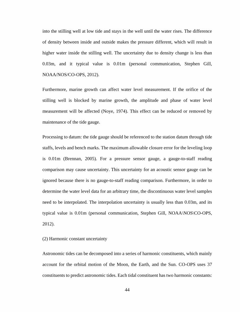
Furthermore, marine growth can affect water level measurement. If the orifice of the
stilling well is blocked by marine growth, the amplitude and phase of water level
measurement will be affected (Noye, 1974). This effect can be reduced or removed by
maintenance of the tide gauge.
Processing to datum: the tide gauge should be referenced to the station datum through tide
staffs, levels and bench marks. The maximum allowable closure error for the leveling loop
is 0.01m (Brennan, 2005). For a pressure sensor gauge, a gauge-to-staff reading
comparison may cause uncertainty. This uncertainty for an acoustic sensor gauge can be
ignored because there is no gauge-to-staff reading comparison. Furthermore, in order to
determine the water level data for an arbitrary time, the discontinuous water level samples
need to be interpolated. The interpolation uncertainty is usually less than 0.03m, and its
typical value is 0.01m (personal communication, Stephen Gill, NOAA\NOS\CO-OPS,
2012).
(2) Harmonic constant uncertainty
Astronomic tides can be decomposed into a series of harmonic constituents, which mainly
account for the orbital motion of the Moon, the Earth, and the Sun. CO-OPS uses 37
constituents to predict astronomic tides. Each tidal constituent has two harmonic constants:

45
amplitude (cm) and phase (degrees). A least square analysis on water level observations
can be performed to derive the harmonic constants, and each harmonic constant has an
associated uncertainty.
Brennan (2005) applied a Monte Carlo simulation to calculate the uncertainties associated
with the harmonic constants for nine stations which vary in latitude and longitude, and tide
types. The range of the uncertainties associated with the harmonic constants for the nine
stations are approximately from 0.02m to 0.25m. The investigation result showed if the
record length used to compute harmonic constants was longer, the associated uncertainty
would be smaller. Therefore, harmonic constant uncertainties for different stations are
different, mainly depending on observation length.
(3) Tidal datum uncertainty
In the U.S. the National Water Level Observation Network (NWLON) is used to acquire
and maintain the tidal datum reference framework. Tidal datums for many NWLON
stations are computed by averaging the water level data over the 19-year NTDE from 1983
to 2001. For a short-term tide station, tidal datum is computed by comparing simultaneous
water level data between the short-term tide station and the appropriate NWLON control
station which is close to the short-term station and has similar tidal characteristics as the
short-term station.
As the tidal datum computation for short-term stations is not based on the full 19-year
NTDE observation, the tidal datum determination will bring in an uncertainty. Bodnar’s
equations (Bodnar, 1981) provide uncertainty estimations of MLW datum determination
from short-term stations:

46
𝑆1 = 0.0021∆𝑡 + 0.0016√𝑑
1852+ 0.0092 |
𝑟𝑐−𝑟𝑠
𝑟𝑐| + 0.0088 (3.6)
𝑆3 = 0.0013∆𝑡 + 0.0011√𝑑
1852+ 0.0078 |
𝑟𝑐−𝑟𝑠
𝑟𝑐| + 0.0088 (3.7)
𝑆6 = 0.0006∆𝑡 + 0.0007√𝑑
1852+ 0.0063 |
𝑟𝑐−𝑟𝑠
𝑟𝑐| + 0.0091 (3.8)
𝑆12 = 0.0025√𝑟𝑐 + 𝑟𝑠 + 0.0390 |𝑟𝑐−𝑟𝑠
𝑟𝑐| + 0.0076 (3.9)
where 𝑆1, 𝑆3, 𝑆6, and 𝑆12 are the standard uncertainty (in meters) for the short-term stations
with one-month, three-month, six-month and 12-month observations respectively, ∆𝑡 is the
time difference of the low water intervals between control and short-term stations (in
hours), d is the geographic distance between control and short-term stations (in meters), 𝑟𝑐
and 𝑟𝑠 are the mean range of tide at the control station and short-term station respectively
(in meters) (Note that the constants and notations in these equations differ from those in
Bodnar (1981), as metric units are used in this thesis).
The equations for MLLW datum are the same as those for MLW datum. Given that
uncertainties for low water datums are higher than those for high water datums (NOAA,
2010), Bodnar’s equations can be used to estimate the uncertainties for all tidal datums,
and the actual uncertainty values should be less than the Bodnar-equation computed values.
According to Bodnar’s equations, tidal datum uncertainty is a function of the time
difference of low water intervals between control and short-term stations, the distance
between control and short-term stations, and the mean tide ranges at control and short-term
stations. In addition, it also depends on the time length of short-term station observation.

47
The longer the short-term station observation is, the smaller the tidal datum uncertainty
will be. For stations with observation longer than one year, the tidal datum uncertainty can
be time-interpolated between the uncertainty estimation for one-year observation and the
zero value for 19-year NTDE observation (NOAA, 2010).
(4) Laplace Equation interpolation uncertainty
TCARI uses the Laplace Equation interpolation method to generate spatial weighting
functions to interpolate: 1) tidal constants for reconstructing astronomic tide; 2) the residual
caused by non-tidal effects; and 3) the datum offsets between Mean Sea Level (MSL) and
MLLW (Cisternelli and Gill, 2005). Then these three components are combined to compute
the water level data at the location of interest.
It is nearly impossible to measure this interpolation uncertainty directly. The interpolation
uncertainty can be determined by comparing the interpolated water level data and the
observed water level data.
Discrete tidal zoning: In the case of a survey area covered by discrete tidal zoning
schemes, because the water level data used to interpolate or extrapolate is the observed
data rather than the data predicted using harmonic constants, the uncertainty sources will
not include harmonic constant uncertainty and Laplace Equation interpolation uncertainty.
Instead, an uncertainty in the application of tidal or water level zoning will be included in
the uncertainty sources (Gibson and Gill, 1999). The water level uncertainty sources for
the direct tidal zoning case include water level observation uncertainty, uncertainty in
computation of tidal datum for the adjustment to a 19-year NTDE from short-term stations,
and uncertainty in the application of tidal or water level zoning.

48
The analyses on water level observation uncertainty and tidal datum uncertainty are the
same as those for TCARI. Like Laplace Equation interpolation uncertainty, uncertainty in
the application of tidal or water level zoning can also be estimated by comparing the
interpolated data and the observed data. A typical uncertainty value associated with tidal
zoning is 0.2 meter at 95% confidence level (personal communication, Stephen Gill,
NOAA/NOS/CO-OPS, 2012). However, in areas with complex and ill-defined tide
characteristics or in areas where meteorology is the major tide forcing, the tidal zoning
uncertainty may dominate the uncertainty in water level data, and its value may exceed 0.2
meter at 95% confidence level.
3.1.4 Human Compilation Uncertainty
The accuracy of human compilation depends on image quality (such as resolution, contrast
and brightness), the compiler’s knowledge about the survey area, the compiler’s shoreline
compilation experience, and the complexity of the survey area. These factors cannot be
quantified simply and thus it is difficult to build an appropriate mathematical model to
describe human compilation uncertainty. Therefore, in this thesis the shoreline compilation
results from different compilers are analyzed to obtain an approximate human compilation
uncertainty value.
The steps for human compilation uncertainty analysis are as follows:
(1) Ask compilers with different experience to interpret a MHW or MLLW shoreline;
(2) Create a reference shoreline using USGS’s Digital Shoreline Analysis System
(DSAS) utility (Thieler et al., 2009);

49
(3) Generate shoreline transects perpendicular to the reference shoreline at a given
interval;
(4) In each transect, calculate the distances between the compiled shorelines and the
reference shoreline;
(5) Obtain the location of the “true” shoreline in each transect by calculating the mean
of the distances calculated in the last step (here the mean of all the compilers’
shorelines is treated as the “true” shoreline);
(6) In each transect, calculate the distances between the compiled shorelines and the
“true” shoreline;
(7) Accumulate statistics of the horizontal offsets (the RMS of the horizontal offsets)
and get the final human compilation uncertainty.
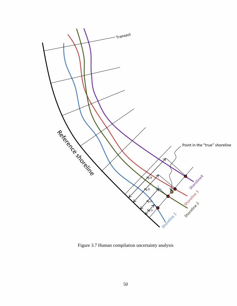
50
Figure 3.7 Human compilation uncertainty analysis
Point in the “true” shoreline
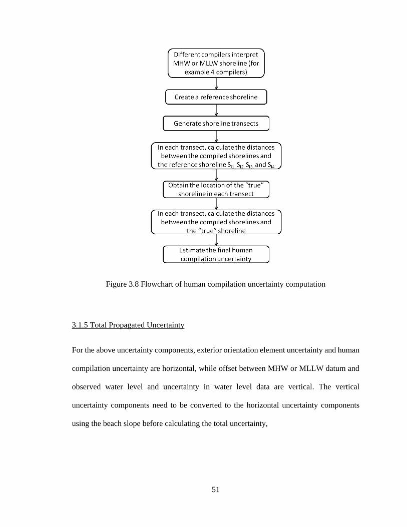
51
Figure 3.8 Flowchart of human compilation uncertainty computation
3.1.5 Total Propagated Uncertainty
For the above uncertainty components, exterior orientation element uncertainty and human
compilation uncertainty are horizontal, while offset between MHW or MLLW datum and
observed water level and uncertainty in water level data are vertical. The vertical
uncertainty components need to be converted to the horizontal uncertainty components
using the beach slope before calculating the total uncertainty,

52
𝑢ℎ =𝑢𝑣
𝑡𝑎𝑛𝜃 (3.10)
where 𝑢𝑣 is a vertical uncertainty component, 𝑢ℎ is the horizontal uncertainty caused by
the vertical uncertainty component, and 𝜃 is the beach slope. The beach slope can be
extracted from a Digital Elevation Model (DEM), for example, using “Spatial Analyst-
>Slope” function in ArcGIS. A vertical uncertainty will cause a greater horizontal
uncertainty in a gentle area than that in a steep area.
Each uncertainty component is assumed to be independent of the others, and so the total
standard uncertainty (at 68% confidence level) and the uncertainty at 95% confidence level
are computed using
𝑢 = 𝑆 + 𝑡68,𝑣𝑅 (3.11)
𝑈95 = 𝑆 + 𝑡95,𝑣𝑅 (3.12)
where 𝑢 is the standard uncertainty (at 68% confidence level); 𝑈95 is the uncertainty at
95% confidence level; 𝑡68,𝑣 is the Student’s t (or coverage factor) for 68% confidence level
and 𝑣 degrees of freedom; 𝑡95,𝑣 is the Student’s t (or coverage factor) for 95% confidence
level and 𝑣 degrees of freedom; when degrees of freedom are infinite, 𝑡68,𝑣 and 𝑡95,𝑣 are 1
and 1.96 respectively; when there are fewer than 30 degrees of freedom, the sample
standard deviation is smaller than the population standard deviation, so Student’s t is used
to compensate for the sample standard deviation (Dieck, 2002); S is the sum of all
systematic uncertainties, and R is the root sum square of all random uncertainties. Offset
between MHW or MLLW datum and the observed water level and tidal datum uncertainty

53
(one source of uncertainty in water level data) are treated as systematic uncertainties, while
the other uncertainty sources are modeled as random uncertainties (Table 3.1).
The degrees of freedom can be obtained (Dieck, 2002):
𝑑. 𝑓. = 𝑣 =[∑ (𝑟𝑖)
2𝑁𝑖=1 +∑ (𝑠𝑗/2)
2𝑀𝑗=1 ]
2
[∑(𝑟𝑖)
4
𝑣𝑖
𝑁𝑖=1 +∑
(𝑠𝑗/2)4
𝑣𝑗
𝑀𝑗=1 ]
(3.13)
where 𝑟𝑖 is the ith random uncertainty (1 ≤ 𝑖 ≤ 𝑁, N is the number of random uncertainty
components), 𝑣𝑖 is the degrees of freedom for the ith random uncertainty, 𝑠𝑗 is the jth
systematic uncertainty component (1 ≤ 𝑗 ≤ 𝑀, M is the number of systematic uncertainty
components), 𝑣𝑗 is the degrees of freedom for the jth systematic uncertainty.
Table 3.1 Uncertainty components for tide-coordinated shoreline
Uncertainty component Uncertainty type
Exterior orientation element uncertainty Random
Offset between MHW or MLLW Datum and Observed Water
Level
Systematic
Uncertainty
in water
level data
TCARI
Water level observation uncertainty Random
Harmonic constant uncertainty Random
Tidal datum uncertainty Systematic
Laplace Equation interpolation
uncertainty
Random
Discrete
tidal
zoning
Water level observation uncertainty Random
Tidal datum uncertainty Systematic
Tidal zoning uncertainty Random

54
Human compilation uncertainty Random
Besides the uncertainty models ((3.11) and (3.12)), there are some other uncertainty models
combining systematic uncertainties and random uncertainties (Dieck, 2002). The reason
why (3.11) and (3.12) are adopted in this thesis is that NOAA is using these two models in
other applications, such as computing uncertainty in water level data, and it is better to
keep the uncertainty models consistent in all of NOAA’s uncertainty computations. In
addition, these two models are conservative in estimating total uncertainty.
The two formulas ((3.11) and (3.12)) can be expressed using each uncertainty source as
follows:
For TCARI:
𝑢 = (𝑢𝑜𝑓 + 𝑢𝑑) + 𝑡68,𝑣√𝑢𝑒2 + 𝑢𝑜𝑏
2 + 𝑢ℎ𝑎2 + 𝑢𝑖
2 + 𝑢ℎ𝑢2 (3.14)
𝑈95 = (𝑢𝑜𝑓 + 𝑢𝑑) + 𝑡95,𝑣 ∗ √𝑢𝑒2 + 𝑢𝑜𝑏
2 + 𝑢ℎ𝑎2 + 𝑢𝑖
2 + 𝑢ℎ𝑢2 (3.15)
For discrete tidal zoning:
𝑢 = (𝑢𝑜𝑓 + 𝑢𝑑) + 𝑡68,𝑣√𝑢𝑒2 + 𝑢𝑜𝑏
2 + 𝑢𝑧2 + 𝑢ℎ𝑢
2 (3.16)
𝑈95 = (𝑢𝑜𝑓 + 𝑢𝑑) + 𝑡95,𝑣√𝑢𝑒2 + 𝑢𝑜𝑏
2 + 𝑢𝑧2 + 𝑢ℎ𝑢
2 (3.17)
where 𝑢𝑒 is exterior orientation element uncertainty; 𝑢𝑜𝑓 is offset between MHW or
MLLW datum and observed water level; 𝑢𝑜𝑏 , 𝑢ℎ𝑎 , 𝑢𝑑 , 𝑢𝑖 and 𝑢𝑧 are water level
observation uncertainty, harmonic constant uncertainty, tidal datum uncertainty, Laplace

55
Equation interpolation uncertainty and tidal zoning uncertainty respectively; and 𝑢ℎ𝑢 is
human compilation uncertainty.
3.2 Shoreline Uncertainty based on Non-Tide-Coordinated Imagery
When shoreline is compiled on non-tide-coordinated imagery, only three main uncertainty
sources contribute to the total uncertainty: (1) exterior orientation element uncertainty; (2)
uncertainty in water level data; and (3) human compilation uncertainty. The offset between
MHW and the observed water level is compensated for in compilation; it is not an
uncertainty component for non-tide-coordinated shoreline. One difference from the tide-
coordinated case is that the photogrammetrist is compiling an elevation contour, as opposed
to a planimetric feature (the land-water interface). Hence, the human compilation
uncertainty is not the same in the two cases.
3.2.1 Exterior Orientation Element Uncertainty
The exterior orientation element uncertainty analysis for non-tide-coordinated shoreline is
the same as that for tide-coordinated shoreline.
3.2.2 Uncertainty in Water Level Data
The analysis of uncertainty in water level for non-tide-coordinated shoreline is the same as
that for tide-coordinated shoreline.
3.2.3 Human Compilation Uncertainty
Because the compilation from the non-tide-coordinated imagery is primarily done based
on elevation information, the human compilation uncertainty for non-tide-coordinated

56
shoreline is analyzed in elevation. The first six steps in human compilation uncertainty
analysis for tide-coordinated shoreline can be used to calculate the horizontal human
compilation uncertainty for non-tide-coordinated shoreline in each transect. The
relationship between the horizontal human compilation uncertainties and the slopes is
linearly fitted using the least square method. The slope of the fitted straight line is the
vertical human compilation uncertainty.
3.2.4 Total Propagated Uncertainty
For the three uncertainty components for non-tide-coordinated shoreline, exterior
orientation element uncertainty is horizontal, while uncertainty in water level data and
human compilation uncertainty are vertical. The vertical uncertainty components need to
be converted to the horizontal uncertainty components using the formula (3.10) before
calculating the total uncertainty.
Table 3.2 Uncertainty components for non-tide-coordinated shoreline
Uncertainty component Uncertainty type
Exterior orientation element uncertainty Random
Uncertainty
in water
level data
TCARI
Water level observation uncertainty Random
Harmonic constant uncertainty Random
Tidal datum uncertainty Systematic
Laplace Equation interpolation
uncertainty
Random
Discrete
tidal
zoning
Water level observation uncertainty Random
Tidal datum uncertainty Systematic
Tidal zoning uncertainty Random

57
Human compilation uncertainty Random
The total standard uncertainty (at 68% confidence level) and the uncertainty at the 95%
confidence level can be expressed using each uncertainty source as follows:
For TCARI:
𝑢 = 𝑢𝑑 + 𝑡68,𝑣√𝑢𝑒2 + 𝑢𝑜𝑏
2 + 𝑢ℎ𝑎2 + 𝑢𝑖
2 + 𝑢ℎ𝑢2 (3.18)
𝑈95 = 𝑢𝑑 + 𝑡95,𝑣√𝑢𝑒2 + 𝑢𝑜𝑏
2 + 𝑢ℎ𝑎2 + 𝑢𝑖
2 + 𝑢ℎ𝑢2 (3.19)
For discrete tidal zoning:
𝑢 = 𝑢𝑑 + 𝑡68,𝑣√𝑢𝑒2 + 𝑢𝑜𝑏
2 + 𝑢𝑧2 + 𝑢ℎ𝑢
2 (3.20)
𝑈95 = 𝑢𝑑 + 𝑡95,𝑣√𝑢𝑒2 + 𝑢𝑜𝑏
2 + 𝑢𝑧2 + 𝑢ℎ𝑢
2 (3.21)

58
CHAPTER 4 – EXPERIMENTAL RESULT
4.1 Shoreline Uncertainty based on Tide-Coordinated Imagery
4.1.1 Exterior Orientation Element Uncertainty
The DSS camera parameters used in this study for estimating the point positioning
uncertainty caused by the exterior orientation element uncertainties include (Applanix,
2014): the flying height over ground, 3048 m; camera focal length, 60.265 mm; pixel size
on CCD chip, 6.8 m; CCD length in the along-track direction, 5408 pixels; CCD length
in the across-track direction, 7212 pixels, and exterior orientation elements of each image
and their standard uncertainties.
Although the computation result will be more accurate with an increase in Monte Carlo
simulation trials, processing time should be taken into account. The first image pair was
tested to determine the number of simulation trials for each image point (100 equally
spaced image points were used from the left image). Figure 4.1 illustrates the relationships
between the number of the simulation trials and X/Y/Z uncertainty caused by exterior
orientation element uncertainties for this image pair. When the number of the simulation

59
trials was greater than 2000, the changes of X, Y and Z uncertainties with the change of the
number of the simulation trials were less than 0.005m, 0.005m and 0.02 m respectively.
Therefore, 2000 simulation trials were implemented for each image point, and in this case
the computation time for the first image pair was about 4 seconds on a Windows PC with
a 2.5 GHz processor and 6 GB of RAM.

60
Figure 4.1 The relationships between the number of the simulation trials and X/Y/Z
uncertainty caused by exterior orientation element uncertainties
For the point positioning uncertainty computation for the whole survey area, the number
of simulation trials for each image point was adjusted based on the number of image pairs:
0 1000 2000 3000 4000 5000 6000 7000 8000 9000 100000.55
0.6
0.65
0.7
0.75
0.8
simulation times
X u
ncert
ain
ty c
aused b
y E
O u
ncert
ain
ty(m
)
0 1000 2000 3000 4000 5000 6000 7000 8000 9000 100000.45
0.5
0.55
0.6
simulation times
Y u
ncert
ain
ty c
aused b
y E
O u
ncert
ain
ty(m
)
0 1000 2000 3000 4000 5000 6000 7000 8000 9000 10000
2.45
2.5
2.55
2.6
2.65
2.7
simulation times
Z u
ncert
ain
ty c
aused b
y E
O u
ncert
ain
ty(m
)

61
2000 divided by the number of image pairs. In this way, an increase in the number of image
pairs barely increases the total computation time and, at the same time, the accuracy of the
point positioning uncertainty computation for the whole survey could be ensured.
The total point positioning uncertainty computation time for this project was about 5
seconds using the same PC. The ground coordinate uncertainties caused by the exterior
orientation element uncertainties are shown in Table 4.1.
Table 4.1 The uncertainty of the ground coordinates caused by the exterior orientation
element uncertainties
X uncertainty 0.61m
Y uncertainty 0.56m
Z uncertainty 2.50m
According to the DRMS formula (3.5), for the whole survey area, the position uncertainty
caused by the exterior orientation element uncertainties was 0.84m.
From the collinearity equations, it can be concluded that the point positioning uncertainty
is determined mainly by the exterior orientation element uncertainties and the photographic
scale at a fixed image overlap (normally the end lap and the side lap are about 60% and
30% respectively). In order to understand how each parameter influences the point
positioning uncertainty, the first image pair (Table 4.2) was selected to do a sensitivity
analysis.
The ranges of the exterior orientation element uncertainties and the photographic scale
were artificially set as follows: exterior orientation line element uncertainty [0, 0.04m];

62
exterior orientation angle element uncertainty [0, 0.02°]; and photographic scale [1:2000,
1:14000]. In this experiment, photographic scale was changed by artificially adjusting the
value of the flying height with the focal length remaining constant. At different
photographic scales, the influence of each exterior orientation element uncertainty on point
positioning uncertainty was analyzed. When computing the point positioning uncertainty
caused by the uncertainty of one exterior orientation element, the uncertainties of the other
exterior orientation elements were set to be 0. Figure 4.2 illustrates the change of the point
positioning uncertainty with the change of the exterior orientation element uncertainties
and the photographic scale.
Table 4.2 The exterior orientation elements of the first image pair
𝑋𝐿 (m) 𝑌𝐿 (m) 𝑍𝐿 (m) 𝜔 (degree) 𝜑 (degree) 𝜅 (degree)
Image 1 645493.401 4969408.741 3013.527 -3.454139 -2.583602 53.705195
Image 2 646016.418 4969954.652 3012.996 -2.179865 -0.140796 53.884717

63

64
Figure 4.2 The influence of the exterior orientation element uncertainties and the
photographic scale on the point positioning uncertainty (for the first image pair)
In addition, an exterior orientation element dataset of an image pair was simulated based
on the first image pair (Table 4.3). The baseline length was the same as that of the first
image pair, which was computed by the exterior orientation line elements of the two
exposure stations, to guarantee their end laps were the same, and the flight direction was
adjusted to be along the X axis. Figure 4.3 illustrates the change of the point positioning
uncertainty with the change of the exterior orientation element uncertainties and the
photographic scale.
Table 4.3 The exterior orientation elements of the simulated image pair
𝑋𝐿 (m) 𝑌𝐿 (m) 𝑍𝐿 (m) 𝜔 (degree) 𝜑 (degree) 𝜅 (degree)
Image 1 645493.401 4969408.741 3013.527 -3.454139 -2.583602 0
Image 2 646249.421 4969408.741 3012.996 -2.179865 -0.140796 0
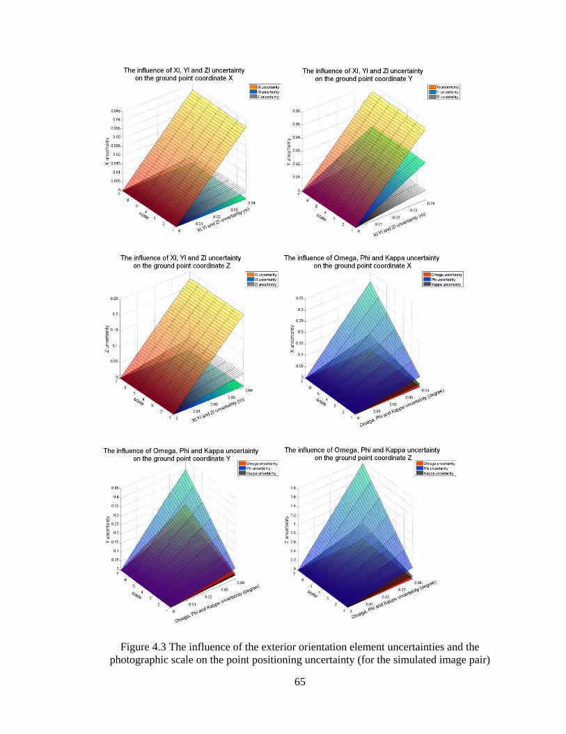
65
Figure 4.3 The influence of the exterior orientation element uncertainties and the
photographic scale on the point positioning uncertainty (for the simulated image pair)

66
The sensitivity analysis results for the exterior orientation element uncertainties and the
photographic scale will be discussed in the next chapter.
4.1.2 Offset between MLLW Datum and Observed Water Level
According to Table 2.2, when the two flightlines (50-001 at 14:06 and 50-002 at 14:18)
were taken, the offsets between the MLLW datum and the observed water level were within
the desired tolerance. The imagery taken along the two flightlines were tide-coordinated
imagery, from which the MLLW lines were interpreted.
The offsets relative to the MLLW datum for both subordinate stations (Coffins Point and
Birch Islands) at 14:06 and 14:18 were analyzed, and the average offset (0.30m) was treated
as the offset between the MLLW datum and the observed water level for the whole survey
area.
4.1.3 Uncertainty in Water Level Data
Firstly, a typical value 0.022 m (personal communication, Lijuan Huang, NOAA/NOS/CO-
OPS/Hydro Planning Team, 2013) was used as the water level observation uncertainty for
the survey area.
Secondly, NGS used the water level data of the EastPort station to analyze water level data
of the two subordinate stations (Coffins Point and Birch Islands). The EastPort station was
established in 1929, and it is a 19-year control station. Therefore, the tidal datum
uncertainty for Eastport was assumed to be zero (NOAA, 2010).
Thirdly, the uncertainty in the application of tidal or water level zoning was analyzed by
comparing the water level data from the Tidal Analysis Report and the prediction based on

67
harmonic constituents, because the harmonic constituents account for more than 99% of
the total water level energy in this region and the predicted data based on harmonic
constituents can be used as alternative observed data to calculate the tidal zoning
uncertainty (personal communication, Lijuan Huang, NOAA/NOS/CO-OPS/Hydro
Planning Team, 2013). CO-OPS provided the predicted data based on harmonic
constituents for Coffins Point and the predicted data based on four time and range
correction parameters for Birch Islands. Therefore, the tidal data for Coffins Point was
analyzed, and its uncertainty was treated as the tidal zoning uncertainty for the whole
survey area. Table 4.4 represents the tidal zoning uncertainty analysis for Coffins Point.
The tidal zoning uncertainty was 0.05 m.
Table 4.4 Tidal zoning uncertainty analysis for Coffins Point
Time
Water level data relative to MLLW
Difference (m)
RMS of differences
(m) From tide analysis
report (m)
Predicted data based on
harmonic constituents
(m)
13:18 0.59 0.66 0.07
0.05
13:24 0.58 0.58 0
14:06 0.27 0.23 0.04
14:18 0.27 0.21 0.06
Because the sample size for tidal zoning uncertainty analysis was only four (3 degrees of
freedom), the sample estimate of standard deviation can be skewed and be smaller than the
population standard deviation.

68
4.1.4 Human Compilation Uncertainty
The shoreline compilation results from four compilers in the 2003 Fort Desoto, Florida
project (Parrish et al., 2005) were applied to analyze the tide-coordinated human
compilation uncertainty due to lack of the tide-coordinated compilation results from
different compilers in the survey area (Maine).
The RMSE for each compiler can be seen to be caused by human compilation uncertainty
and all the other factors. The average of the four compilers’ compilation offsets against the
GPS ground truth was treated as the uncertainty caused by all other factors except for the
human compilation uncertainty. Table 4.5 shows the human compilation uncertainty
analysis based on the four compilers’ compilations.
Table 4.5 Tide-coordinated human compilation uncertainty computation
(The mean and RMSE of each compiler were obtained by comparing land/water interface
and the GPS ground truth. The negative mean uncertainty means a seaward offset against
the GPS ground truth)
Shoreline Mean (m) RMSE (m) √𝑅𝑀𝑆𝐸2 − 𝐴𝑣𝑒𝑟𝑎𝑔𝑒2 Human compilation uncertainty
(m)
(RMS of the fourth column)
Compiler 1 -0.59 0.94 0.33
1.06
Compiler 2 -1.56 1.94 1.73
Compiler 3 -0.39 0.92 0.27
Compiler 4 -0.98 1.45 1.15
Average -0.88
The human compilation uncertainty was found to be 1.06 m. Like the tidal zoning
uncertainty analysis, the sample size of the tide-coordinated human compilation
uncertainty analysis was also very small (3 degrees of freedom). Therefore, the population

69
standard deviation of the tide-coordinated human compilation uncertainty can be greater
than 1.06m. In addition, given that the coastal area in the Maine site is more complex than
that in Fort Desoto and there are more types of shorelines in the Maine site, the human
compilation uncertainty for the Maine site may be greater than that for Fort Desoto.
Therefore, it is reasonable to suppose that 1.06m underestimated the tide-coordinated
human compilation uncertainty for the Maine site.
4.1.5 Total Propagated Uncertainty
Among the above four uncertainty components, the offset between the MLLW datum and
the observed water level and the uncertainty in water level data are vertical uncertainty
components, while the exterior orientation uncertainty and the human compilation
uncertainty are horizontal uncertainty components. All vertical uncertainty components
should be converted to the horizontal uncertainty components using the beach slope before
calculating the total uncertainty.
The beach slope was extracted from LiDAR data using ArcGIS. The slope raster imagery
was then processed by a smoothing (low pass) filter, which calculated the average value
for each 3 × 3 neighborhood. The high and low values within each neighborhood were
averaged out, reducing the extreme values of the beach slopes (Figure 4.4).

70
Figure 4.4 Filtered slope raster imagery
After obtaining the beach slope, the reference shorelines were firstly created, and then
transects at the interval of 2m along shorelines were generated using DSAS. On each
transect, the vertical uncertainty components were converted to horizontal uncertainty
components.
The degrees of freedom for the tidal zoning uncertainty and the human compilation
uncertainty were 3, and the degrees of freedom for all the other uncertainty components
were assumed to be infinite. The degrees of freedom for the total uncertainty were
computed using the value of each uncertainty component and their degrees of freedom
according to (3.13), then the total standard uncertainty and the uncertainty at the 95%
confidence level were estimated according to (3.16) and (3.17). The RMSs of the
uncertainties on all the transects were the total uncertainties for the whole survey area:
3.28m total standard uncertainty and 4.77m uncertainty at the 95% confidence level.

71
4.2 Shoreline Uncertainty based on Non-Tide-Coordinated Imagery
4.2.1 Exterior Orientation Element Uncertainty
The point positioning uncertainty caused by the exterior orientation element uncertainties
for non-tide-coordinated shoreline is the same as that for tide-coordinated shoreline.
4.2.2 Uncertainty in Water Level Data
The value of the uncertainty in water level data for non-tide-coordinated shoreline is the
same as that for tide-coordinated shoreline.
4.2.3 Human Compilation Uncertainty
Nine compilers with different experience levels compiled the MHW lines from non-tide-
coordinated imagery in the two regions selected from the survey area (8 degrees of
freedom), and the compilation results were analyzed to determine the non-tide-coordinated
human compilation uncertainty.
Two reference shorelines were first created, and then shoreline transects were generated
perpendicular to the reference shorelines at 10 m spacing (Figure 4.5). The average of the
compiled shorelines was treated as the shorelines without human compilation uncertainty,
and then the RMS of all the compilers’ uncertainties was computed in each transect as the
human compilation uncertainty of this transect.

72
Figure 4.5 The reference shorelines (red lines) and transects (blue lines). Different colors
in transects represent the degree of the maximum difference of the compilation results
from the compilers.
Combined with the slope information along the two shorelines, the planimetric human
compilation uncertainty was converted to uncertainty in elevation. Figure 4.6 illustrates the
relationship between the slope and the planimetric human compilation uncertainty. From
the distribution of the points, it can be seen that the horizontal human compilation
uncertainty from non-tide-coordinated imagery depends on the beach slope, because
compilers compile the shoreline based on the elevation information. When the vertical
human compilation uncertainty is fixed, the horizontal human compilation uncertainty will
change with the beach slope.

73
Figure 4.6 The relationship between the slope and the planimetric human compilation
uncertainty
The black line is the least-square fitted straight line based on the data of planimetric human
compilation uncertainty and the slope. The slope of this fitted straight line, 0.44 m, was
used as the elevation uncertainty corresponding to this level of planimetric compilation
uncertainty.
4.2.4 Total Propagated Uncertainty
Among the above three uncertainty components, the uncertainty in water level data and the
human compilation uncertainty are vertical uncertainty components, while the exterior
orientation uncertainty is a horizontal uncertainty component.
On each transect, the vertical uncertainty components were converted to horizontal
uncertainty components. Here, the degrees of freedom for the tidal zoning uncertainty and
the human compilation uncertainty were 3 and 8 respectively, and the degrees of freedom
for all the other uncertainty components were assumed to be infinite. The degrees of
/通用格式
/通用格式
/通用格式
/通用格式
/通用格式
/通用格式
/通用格式
0 5 10 15 20
pla
nim
etr
ic u
nce
rtai
nty
(m)
1/tan(slope)

74
freedom for the total uncertainty were computed using the value of each uncertainty
component and their degrees of freedom according to (3.13), then the total standard
uncertainty and the uncertainty at the 95% confidence level were computed according to
(3.20) and (3.21). The RMSs of the uncertainties on all the transects were the total
uncertainties for the whole survey area: the total standard uncertainty was 3.15m and the
uncertainty at the 95% confidence level was 6.73m.
The boundaries for the standard uncertainty and the uncertainty at the 95% confidence level
are shown on the imagery (Figure 4.7).
Figure 4.7 The uncertainty boundaries. The blue lines and the red lines represent the
standard uncertainty and the uncertainty at the 95% confidence level respectively. The
black lines are the MHW shoreline. (Left) the imagery for the whole survey area. (Right)
the enlarged imagery for the yellow box in the left imagery; the points with different
colors represent the slope in degrees.

75
From Figure 4.7 (right), it can be seen that in a region with gentle slope the uncertainty is
greater than that in a steep region. It can be concluded slope is an important factor which
affects the shoreline uncertainty.
76
CHAPTER 5 – DISCUSSION
5.1 Exterior Orientation Element Uncertainty
In the experiment, the simulation times of each pair of corresponding image points were
dynamically adjusted based on the number of the image pairs (2000 divided by the number
of the image pairs), and the experiment result showed that the computation time and the
accuracy were both acceptable.
The sensitivity analysis of exterior orientation element uncertainties and photographic
scale (Figure 4.2 and Figure 4.3) led to the following conclusions:
(1) The point positioning uncertainty increases linearly with the increase of the exterior
orientation element uncertainties.
(2) The point positioning uncertainty caused by the exterior orientation angle element
uncertainties (𝜎𝜔, 𝜎𝜑, 𝜎𝜅) is affected linearly by the photographic scale. The smaller
the scale is, the higher the point positioning uncertainty and the greater the change
of the point positioning uncertainty with the change of the exterior orientation angle
element uncertainties. On the other hand, the photographic scale has negligible
impact on the point positioning uncertainty caused by the exterior orientation line
element uncertainties (𝜎𝑋𝐿, 𝜎𝑌𝐿
, 𝜎𝑍𝐿).
(3) The uncertainties of 𝑋𝐿 and 𝜑 mainly affect the accuracy of the ground point
coordinate X, and the uncertainties of 𝑌𝐿 and 𝜔 mainly affect the accuracy of the

77
ground point coordinate Y. However, it is important to note that these observations
depend on the orientation of the flight lines with respect to true north (or the axes
of the mapping frame). If the flight direction is closer to the X axis (Y axis), the
uncertainties of 𝑋𝐿 and 𝜑 ( 𝑌𝐿 and 𝜔 ) have greater influence on the point
positioning accuracy.
5.2 Tidal Zoning Uncertainty
The water level data for Coffins Point at the only four different times (Table 4.4) was
applied to analyze the tidal zoning uncertainty for the survey area. The sample size is so
small that the tidal zoning uncertainty value from this analysis may have underestimated
the actual tidal zoning uncertainty. According to the values of the Student’s t for 4 and
infinite sample sizes at 68% confidence level, it would be expected that the value of the
actual tidal zoning uncertainty is ~1.2 times that of the tidal zoning uncertainty estimated
by the 4 samples.
5.3 Human Compilation Uncertainty
The human compilation uncertainty was estimated by analyzing compilation results from
different compilers. The estimated values for the two cases (tide-coordinated and non-tide-
coordinated) cannot be easily applied to any area or any set of compilers, and they should
be adjusted based on different conditions, such as compiler’s experience, image quality
and complexity of coastal region.
78
The compilation results from four compilers in Fort Desoto were applied to estimate the
tide-coordinated human compilation uncertainty for the Maine site. However, the
topography of the Maine site is more complex than that of Fort Desoto. Therefore, the
human compilation uncertainty for Fort Desoto may have underestimated that for Maine.
In addition, the small sample sizes for the tide-coordinated and non-tide-coordinated
human compilation uncertainty analysis may have resulted in the sample human
compilation uncertainties being less than the population human compilation uncertainties.
According to the values of the Student’s t for 4, 9 and infinite sample sizes at 68%
confidence level, it would be expected that the value of the actual tide-coordinated human
compilation uncertainty for the Maine site is greater than ~1.2 times that of the tide-
coordinated human compilation uncertainty estimated by the 4 Fort Desoto compilation
samples, and the value of the actual non-tide-coordinated human compilation uncertainty
is ~1.06 times that of the non-tide-coordinated human compilation uncertainty estimated
by the 9 Maine compilation samples.
5.4 Comparison of Tide-Coordinated and Non-Tide-Coordinated Uncertainties
Table 5.1 provides the planimetric values of each uncertainty component and the total
uncertainties for this shoreline survey.
From this table, it can be seen that for tide-coordinated compilation the offset between
MHW/MLLW and observed water level has the main impact on the total uncertainty,
followed by human compilation uncertainty, exterior orientation element uncertainty, and
then uncertainty in water level data. For non-tide-coordinated compilation, the order is

79
human compilation uncertainty, exterior orientation element uncertainty, and then
uncertainty in water level data. In addition, the non-tide-coordinated human compilation
uncertainty is greater than the tide-coordinated one. Comparing the total uncertainties for
the two cases, they are not very different from each other. This indicates that it may not be
necessary to require a survey to be tide-coordinated. However, the shoreline TPU would
need to be computed for many survey sites to determine if this is true in general, or only
for this particular survey.
Table 5.1 The planimetric values (in meters) of each uncertainty component and the total
uncertainties for the survey area (The tidal zoning uncertainty and the human compilation
uncertainty were computed using their sample uncertainty values multiplied by their
corresponding Student’s t)
Exterior
orientation
element
uncertainty
The offset
between
MHW or
MLLW datum
and observed
water level
Uncertainty in water level data Human
compilation
uncertainty
Total uncertainty
Observation Datum Zoning Std 95% Cl
Tide-
coordinated
0.84 1.96 0.15 0 0.39 1.26 3.28 4.77
Non-tide-
coordinated
0.84 0 0.15 0 0.39 3.03 3.15 6.73
5.5 Relationship between Uncertainty and Slope
For the study area, the ranges of the standard uncertainties for tide-coordinated and non-
tide-coordinated compilation along the different transects are [1.72m, 31.20m] and [0.93m,
40.78m] (Figure 5.1). The variability in the uncertainty is primarily attributable to slope
variation (Figure 5.2). In areas with small slope, the uncertainty is higher. The upper limits
of these TPU ranges are quite large. However, they are realistic, since in some sections of
the study area the beach slope is extremely small, such as 0.66°. These upper limits of the
uncertainty ranges should not be taken as a reflection of the standard uncertainty for the

80
study area as a whole, but it is important to note that the uncertainty in a few localized areas
can be significantly greater than the standard shoreline uncertainty for the survey area.
Figure 5.1 Distribution of standard uncertainties for tide-coordinated and non-tide-
coordinated compilation
0 5 10 15 20 25 30 350
0.02
0.04
0.06
0.08
0.1
0.12
0.14
0.16
0.18
0.2
Pro
babili
ty d
ensity
Standard uncertainty for tide-coordinated compilation (m)
0 5 10 15 20 25 30 35 40 450
0.02
0.04
0.06
0.08
0.1
0.12
0.14
0.16
0.18
0.2
Pro
babili
ty d
ensity
Standard uncertainty for non-tide-coordinated compilation (m)

81
Figure 5.2 Distribution of slopes
0 5 10 15 20 25 30 35 40 45 500
0.005
0.01
0.015
0.02
0.025
0.03
0.035
Pro
babili
ty d
ensity
Slope (degrees)

82
CHAPTER 6 – CONCLUSIONS AND RECOMMENDATIONS
FOR FUTURE WORK
The photogrammetric method for shoreline mapping has many advantages: maturity,
capability of mapping large areas with great detail quickly, access to certain areas where
field surveys are infeasible, and good accuracy for man-made/built-up shorelines.
Therefore, it has been the main shoreline mapping method used by NGS since 1927.
Compared with the development of this technique, the statistical method of estimating the
photogrammetry-derived shoreline uncertainty has lagged behind. This thesis therefore
proposes a TPU model in order to generate metadata containing accuracy for the national
shoreline, which will make the shoreline product more useful. The uncertainty boundaries
generated based on the uncertainty values in ArcGIS enable users to understand the
shoreline uncertainty visually.
In addition to providing the shoreline metadata, this TPU model can also be used before a
survey to judge whether a given accuracy requirement can be met based on the accuracy
of the integrated GPS/IMU system, photographic scale, predicted water level, human
compilation uncertainty and other factors. This analysis, if conducted in advance of a
survey, can be used to modify acquisition procedures to maximize efficiency and ensure
adherence to applicable specifications.

83
Through the uncertainty analysis for the study area (northeast coast of Maine), it can be
seen that the total uncertainties for tide-coordinated shoreline compilation and non-tide-
coordinated shoreline compilation are similar. This suggests that, if the pre-survey
uncertainty estimation meets the accuracy requirement, survey time can be determined
based on weather conditions, and does not necessarily have to be tide-coordinated.
In addition, from the experiment results it can be concluded that the offset between
MHW/MLLW datum and observed water level is the most important uncertainty
component for tide-coordinated shoreline compilation, and for non-tide-coordinated
shoreline compilation human compilation uncertainty is most significant. In order to
efficiently reduce the total uncertainty, for tide-coordinated shoreline compilation aerial
imagery should be taken at the time when predicted water level is closer to MHW/MLLW
datum, and for non-tide-coordinated shoreline compilation, the level of the compiler’s
experience is critical.
However, there are still several topics which need to be examined in future research,
including:
(1) The human compilation uncertainty was estimated by analyzing compilation
results from different compilers. The estimated values for the two cases (tide-
coordinated and non-tide-coordinated) cannot be easily applied to another area
or set of compilers, and they should be adjusted based on different conditions.
In fact, this uncertainty should be estimated as a function of additional
variables, including the compiler’s experience, complexity of the coast, and
image quality. Modeling human compilation uncertainty should be one of the

84
important goals for future work, including how to judge the compiler’s
experience, complexity of the coast, and image quality, and how to weigh these
factors in one model. From the model, we would like to determine how each
factor influences the human compilation uncertainty and the range of this
uncertainty.
(2) This TPU model should be tested in different sites. This would enable analysis
of how each uncertainty component and the total uncertainty change in different
conditions.
(3) There are several techniques for shoreline mapping. Some of them are being
used by NGS, and some of them are being explored. It is necessary to compare
the uncertainties of different techniques. A comprehensive analysis of these
techniques should be performed, including uncertainty, constraints (such as that
a photogrammetric shoreline survey cannot be conducted at night), and cost
both in terms of time and money. This would be useful in choosing an
appropriate technique for a specific shoreline mapping project.

85
LIST OF REFERENCES
Alfugura, A., L. Billa, and B. Pradhan, 2011. Semi-automated procedures for shoreline
extraction using single RADARSAT-1 SAR image. Estuarine, Coastal and Shelf
Science 95(4), 395-400.
Applanix, 2013. POSPac MMS.
http://www.applanix.com/products/airborne/pospacmms.html. (accessed October
28, 2013).
Applanix, 2014. DSS 439 Specification.
http://www.applanix.com/media/downloads/products/specs/DSS%20439%20Specs.
pdf. (accessed April 09, 2014)
Boak, E.H., and I.L. Turner, 2005. Shoreline definition and detection: a review. Journal
of Coastal Research 21(4), 688-703.
Bodnar, A.N., 1981. Estimating accuracies of tidal datums from short term observations,
draft report, Tides and Water Levels Division, NOAA National Ocean Survey.
Brennan L., 2005. An uncertainty model for the tidal constituent and residual
interpolation (TCARI) method of water level correction. Master’s thesis, University
of New Hampshire, Durham, NH.
Brock, J.C. and S.J. Purkis, 2009. The emerging role of Lidar remote sensing in
coastalresearch and resource management. Journal of Coastal Research, 53, 1–5.
Cisternelli M. and G. Stephen, 2005. Implementation of TCARI into NOS Hydrographic
Survey Operations. U.S. Hydro, San Diego, California, March 29-31.
Coastal Services Center, 2013. Digital Coast, Coastal Lidar.
https://csc.noaa.gov/digitalcoast/data/coastallidar. (accessed July 25, 2013).

86
CO-OPS, 2014. Tides&Currents: Tides/Water Levels for 8410140 Eastport, ME
2011/06/21.http://tidesandcurrents.noaa.gov/waterlevels.html?id=8410140&units=
metric&bdate=20110621&edate=20110621&timezone=GMT&datum=MLLW&int
erval=6&action=data. (accessed February 28, 2014).
Creel, L., 2003. Ripple effects: population and coastal regions. Measure communication,
September 2003. Population Reference Bureau, Washington, pp 1–7.
Crossett, K. M., T. J. Culliton, P. C. Wiley, and T. R. Goodspeed, 2004. Population
Trends Along the Coastal United States: 1980- 2008. National Oceanic and
Atmospheric Administration (NOAA), National Ocean Service.
http://oceanservice.noaa.gov/programs/mb/pdfs/coastal_pop_trends_complete.pdf
(accessed January 22, 2014).
Dieck, R.H., 2002. Measurement Uncertainty: Methods and Applications, Third Edition.
ISA, The Instrumentation, Systems and Automation Society, 252p.
Filin, S., 2001. Calibration of Airborne and Spaceborne Laser Altimeters Using Natural
Surfaces, Ph.D. thesis, The Ohio State University, Columbus, Ohio.
Gibson, W.M. and S.K. Gill. 1999. Tides and Water Level Requirements for NOS
Hydrographic Surveys. International Hydrographic Review, Monaco, LXXVI(2),
September 1999.
Graham, D., M. Sault, and J. Bailey, 2003. National ocean service shoreline- past,
present, and future. Journal of Coastal Research, SI(38), 14-32.
Grejner-Brzezinska, D.A., 1999. Direct exterior orientation of airborne imagery with
GPS/INS system: Performance analysis. Navigation, 46(4): 261-270.
Hutchins, P.S. and S. Oivanki, 1994. A Comparison of shoreline measurement
techniques: GPS survey, air photo interpretation, and total station survey [abs].
Journal of the Mississippi Academy of Sciences, 39(1), 48.
IHO (International Hydrographic Organization), 2008. IHO Standards for Hydrographic
Surveys, 5th edition. Monaco: International Hydrographic Bureau, 36p.

87
Kinexxions, 2014. The Tides at Cobscook Bay.
http://kinexxions.blogspot.com/2012/10/the-tides-at-cobscook-bay.html (accessed
February 27, 2014).
Leigh, G.E., T. Blackford, and etc., 2012. Scope of Work for Shoreline Mapping under
the NOAA Coastal Mapping Program (14A),
http://www.ngs.noaa.gov/ContractingOpportunities/CMPSOWV14A_FINAL.pdf
(accessed January 29, 2014).
Lindenberger, J., 1989. Test results of laser profiling for topographic terrain survey.
Proceedings of the 42nd Photogrammetric Week, Stuttgart, Germany.
Liu H.X., D. Sherman, and S. Gu, 2007. Automated Extraction of Shorelines from
Airborne Light Detection and Ranging Data and Accuracy Assessment Based on
Monte Carlo. Journal of Coastal Research, 23(6): 1359-1369.
Manual, D.F., 2007. Digital Elevation Model Technologies and Applications: The DEM
Users Manual, 2nd Edition. American Society of Photogrammetry and Remote
Sensing, 655p.
McGlone, J.C., Mikhail E.M., Bethel J., and Mullen R., 2004. Manual of
Photogrammetry Fifth Edition. American Society of Photogrammetry and Remote
Sensing, 1151p.
Mikhail, E., J. Bethel, and J. McGlone, 2001. Introduction to modern photogrammetry.
John Wiley & Sons, New York, 479 p.
Mostafa M. M.R., J. Hutton, and E. Lithopoulos, 2001. Airborne Direct Georeferencing
of Frame Imagery: An Error Budget. The 3rd International Symposium on Mobile
Mapping Technology, Cairo, Egypt, January 3-5.
NGS, 2014a. NGS Shoreline Mapping History.
http://www.ngs.noaa.gov/web/about_ngs/history/NGSshoreline.shtml . (accessed
January 23, 2014).
NGS, 2014b. Coastal and Shoreline Change Analysis Program.
http://www.ngs.noaa.gov/RSD/cscap.shtml . (accessed February 24, 2014)

88
NGS, 2014c. Synthetic Aperture Radar (SAR).
http://www.ngs.noaa.gov/RESEARCH/RSD/main/sar/sar.shtml. (accessed February
24, 2014)
NGS, 2014d. NOAA Shoreline Data Explorer. http://www.ngs.noaa. gov/NSDE/
(accessed February 28, 2014).
National Ocean Service (NOS), 2014. Transformations in Coastal Mapping: 1987- 2007.
http://celebrating200years.noaa.gov/transformations/mapping/#map (accessed
February 4, 2014).
NOAA, 2010. Technical considerations for use of geospatial data in sea level change
mapping and assessment. Silver Spring, Maryland: National Oceanic and
Atmospheric Administration, National Ocean Service, NOAA Technical Report
NOS 2010-01, 130p.
NOAA Fisheries, 2014. Greater Atlantic Region (formerly Northeast Region)
http://www.nero.noaa.gov/stories/2013/boilingtidesnewenergysource.html
(accessed February 27, 2014).
Noye, B.J., 1974. Tide-well systems I: some non-linear effects of conventional tide well.
Journal of Marine Research, 32(2): 129-135.
Office of Coast Survey, 2013a. Datums and transformations.
http://www.nauticalcharts.noaa.gov/csdl/learn_datum.html (accessed February 01
2013).
Office of Coast Survey, 2013b. Chart 13394.
http://www.charts.noaa.gov/OnLineViewer/13394.shtml (accessed October 25,
2013).
Office of Coast Survey, 2013c. Tidal corrector application (TCARI).
http://www.nauticalcharts.noaa.gov/csdl/tcari.html (accessed October 29, 2013).
Office of Coast Survey, 2013d. Field Procedures Manual.
http://www.nauticalcharts.noaa.gov/hsd/fpm/FPM_2013_Final_5_3_13.pdf
(accessed October 29, 2013).

89
Office of General Counsel, NOAA, 2014. Maritime Zones and Boundaries.
http://www.gc.noaa.gov/gcil_maritime.html. (accessed April 16, 2014)
Pajak, M.J., and S.P. Leatherman, 2000. The high water line as shoreline indicator.
Journal of Coastal Research, 18(2): 329-337.
Papadopoulos, C.E. and Yeung, H., 2001. Uncertainty estimation and Monte Carlo
simulation method. Flow Measurement and Instrument, 12, 291–298.
Parrish, C.E., M. Sault, S.A. White, and J. Sellars, 2005. Empirical analysis of aerial
camera filters for shoreline mapping. Proceedings of the ASPRS 2005 Annual
Conference, 7-11 March, Baltimore, MD.
Parrish, C.E., 2011. Shoreline Uncertainty-Motivation and Research Objective. Parrish,
C. 2011 CCOM Progress Report.
Parrish, C.E., 2012. Shoreline Mapping, in Advances in Mapping from Remote Sensor
Imagery: Techniques and Applications, CRC Press, (X. Yang and J. Li, Eds.),
Taylor and Francis Group, Boca Raton, Florida, pp. 145- 168.
Pe’eri, S., C.E. Parrish, C. Azuike, L. Alexander, and A.A. Armstrong, 2014. Satellite
Remote Sensing as a Reconnaissance Tool for Assessing Nautical Chart Adequacy
and Completeness, Marine Geodesy. (Submitted)Royal Swedish Academy of
Sciences, 2012. Sea Level Changes Report.
http://www.kva.se/Documents/Vetenskap_samhallet/Energi/Utskottet/2012/rapport
_energi_havsvattenstand_eng_2012.pdf (accessed January 22, 2014).
Philpot, W.D., 2012. Photogrammetry, Remote Sensing Fundamentals.
http://ceeserver.cee.cornell.edu/wdp2/cee6100/6100_monograph/mono_07_F12_ph
otogrammetry.pdf (accessed February 22, 2014).
Porter, D. L. and H. H. Shih, 1996. Investigations of temperature effects on NOAA's next
generation water level measurement system. Journal of Atmospheric and Oceanic
Technology, 13(3):714-725.
Royal Swedish Academy of Sciences, 2012. Sea Level Changes Report.
http://www.kva.se/Documents/Vetenskap_samhallet/Energi/Utskottet/2012/rapport
_energi_havsvattenstand_eng_2012.pdf (accessed January 22, 2014).

90
Shalowitz, A.L., 1964. Shore and sea boundaries. U.S. Department of Commerce, U.S.
Coast and Geodetic Survey.
Shih, H.H., D.H. Deitemyer and M.W. Allen, (1984). Field Evaluation of a New Tide
Gage Stilling Well Design. Proc. 3rd International Offshore Mechanics and Arctic
Engineering, New Orleans, LA, V. II, pp. 98-105.
Shih, H.H., 1986. Design of Bubble Water Level Gauges for Dynamic Environment.
Proc. 9th Ann. Energy-Sources Technology Conference, New Orleans, LA, pp. 411-
418.
Shih, H.H. and L. Baer, 1991. Some Errors in Tide Measurement Caused by Dynamic
Environment. Tidal Hydrodynamics, B.B. Parker (Ed.), John Wiley & Sons, Inc.,
pp. 641-671.
Smith, J.T., 1981. A History of Flying and Photography in the Photogrammetry Division
of the National Ocean Survey, 1919-79. US Department of Commerce,
Washington, D.C., 99.
Schwarz, K.P, M. A. Chapman, M. W. Cannon, and P. Gong, 1993. An integrated
INS/GPS approach to the georeferencing of remotely sensed data. Photogrammetric
engineering and remote sensing, 59(11), 1667-1674.
Stockdon, H.F., A.H. Sallenger, J.H. List, and R.A. Holman, 2002. Estimation of
shoreline position and change using airborne topographic Lidar Data. Journal of
Coastal Research, 18, 502-513.
Thieler, E.R., E.A. Himmelstoss, J.L. Zichichi, and A. Ergul, 2009. Digital Shoreline
Analysis System (DSAS) version 4.0- An ArcGIS extension for calculating
shoreline change, U.S. Geological Survey Open-File Report 2008-1278.
Vaughn, C.R., J.L. Bufton, W.B. Krabill, and D. Rabine, 1996. Georeferencing of
airborne laser altimeter measurements. International Journal of Remote Sensing,
17(11), 2185–2200.
Wainwright, D.B., 1922. Plane Table Mapping. Department of Commerce, U.S. Coast
and Geodetic Survey, 97p.

91
White, S.A., C.E. Parrish, B.R. Calder, S. Pe’eri and Y. Rzhanov, 2011. Lidar-derived
national shoreline: empirical and stochastic uncertainty analyses, Journal of Coastal
Research, SI(62), 62-74.
Woodlard, J.W., M. Aslaksen, J.LT Longenecker, and A. Ryerson, 2003. Shoreline
mapping from airborne LiDAR in Shilshole Bay, Washington. Proceedings of
National Oceanic and Atmospheric Administration (NOAA) National Ocean Service
(NOS), U.S. Hydrographic Conference.
World Resources Institute (WRI). 2000. World Resources: 2000-2001. Washington, DC:
WRI.
Wozencraft, J., and D. Millar, 2005. Airborne lidar and integrated technologies for
coastal mapping and nautical charcting. Marine Technology Society Journal. 39(3),
27–35.
Xu D., H. Xue, D.A. Greenberg, 2006. A Numerical Study of the Circulation and Drifter
Trajectories in Cobscook Bay. Proceedings of the 9th International Conference on
Estuarine and Coastal Modeling, Charleston, South Carolina, pp. 176- 194.
Yuan X.X., X.P. Zhang, 2008. Theoretical accuracy of direct georeferencing with
position and orientation system in aerial photogrammetry. The International
Archives of the Photogrammetry, Remote Sensing and Spatial Sciences, Beijing,
37(B1): 617-622.
Zhang, X.P., and X.X. Yuan, 2008. Effects of Exterior Orientation Elements on Direct
Georeferencing in POS-Supported Aerial Photogrammetry. Proceedings of the 8th
International Symposium on Spatial Accuracy Assessment in Natural Resources
and Environmental Sciences, Shanghai, June 25-27: 30-36.

92
APPENDIX: TIDE ANALYSIS REPORT FOR ME1001

93
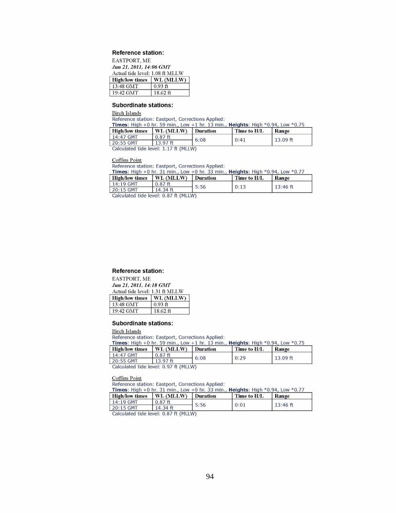
94