uncertain outcomes and climate change policy€¦ · uncertain outcomes and climate change policy...
TRANSCRIPT
UNCERTAIN OUTCOMES AND CLIMATE
CHANGE POLICY
Robert S. Pindyck
Massachusetts Institute of Technology
FEEMJune 3, 2010
Robert Pindyck (MIT) CLIMATE CHANGE POLICY June 2010 1 / 37

Introduction
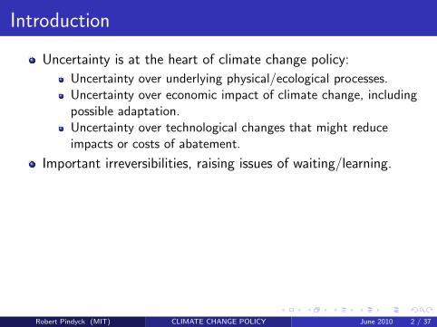
Uncertainty is at the heart of climate change policy:
Uncertainty over underlying physical/ecological processes.Uncertainty over economic impact of climate change, includingpossible adaptation.Uncertainty over technological changes that might reduceimpacts or costs of abatement.
Important irreversibilities, raising issues of waiting/learning.
GHG concentrations decay very slowly.Abatement policy imposes sunk costs.
Long time horizon – around 100 years. How to discount?
What does uncertainty, and especially low-probability extremeoutcomes, imply for climate change policy?
Willingness to Pay (WTP): What fraction of current and futureconsumption would society give up to keep ∆T low?
Robert Pindyck (MIT) CLIMATE CHANGE POLICY June 2010 2 / 37

Introduction
Uncertainty is at the heart of climate change policy:
Uncertainty over underlying physical/ecological processes.
Uncertainty over economic impact of climate change, includingpossible adaptation.Uncertainty over technological changes that might reduceimpacts or costs of abatement.
Important irreversibilities, raising issues of waiting/learning.
GHG concentrations decay very slowly.Abatement policy imposes sunk costs.
Long time horizon – around 100 years. How to discount?
What does uncertainty, and especially low-probability extremeoutcomes, imply for climate change policy?
Willingness to Pay (WTP): What fraction of current and futureconsumption would society give up to keep ∆T low?
Robert Pindyck (MIT) CLIMATE CHANGE POLICY June 2010 2 / 37

Introduction
Uncertainty is at the heart of climate change policy:
Uncertainty over underlying physical/ecological processes.Uncertainty over economic impact of climate change, includingpossible adaptation.
Uncertainty over technological changes that might reduceimpacts or costs of abatement.
Important irreversibilities, raising issues of waiting/learning.
GHG concentrations decay very slowly.Abatement policy imposes sunk costs.
Long time horizon – around 100 years. How to discount?
What does uncertainty, and especially low-probability extremeoutcomes, imply for climate change policy?
Willingness to Pay (WTP): What fraction of current and futureconsumption would society give up to keep ∆T low?
Robert Pindyck (MIT) CLIMATE CHANGE POLICY June 2010 2 / 37

Introduction
Uncertainty is at the heart of climate change policy:
Uncertainty over underlying physical/ecological processes.Uncertainty over economic impact of climate change, includingpossible adaptation.Uncertainty over technological changes that might reduceimpacts or costs of abatement.
Important irreversibilities, raising issues of waiting/learning.
GHG concentrations decay very slowly.Abatement policy imposes sunk costs.
Long time horizon – around 100 years. How to discount?
What does uncertainty, and especially low-probability extremeoutcomes, imply for climate change policy?
Willingness to Pay (WTP): What fraction of current and futureconsumption would society give up to keep ∆T low?
Robert Pindyck (MIT) CLIMATE CHANGE POLICY June 2010 2 / 37

Introduction
Uncertainty is at the heart of climate change policy:
Uncertainty over underlying physical/ecological processes.Uncertainty over economic impact of climate change, includingpossible adaptation.Uncertainty over technological changes that might reduceimpacts or costs of abatement.
Important irreversibilities, raising issues of waiting/learning.
GHG concentrations decay very slowly.
Abatement policy imposes sunk costs.
Long time horizon – around 100 years. How to discount?
What does uncertainty, and especially low-probability extremeoutcomes, imply for climate change policy?
Willingness to Pay (WTP): What fraction of current and futureconsumption would society give up to keep ∆T low?
Robert Pindyck (MIT) CLIMATE CHANGE POLICY June 2010 2 / 37

Introduction
Uncertainty is at the heart of climate change policy:
Uncertainty over underlying physical/ecological processes.Uncertainty over economic impact of climate change, includingpossible adaptation.Uncertainty over technological changes that might reduceimpacts or costs of abatement.
Important irreversibilities, raising issues of waiting/learning.
GHG concentrations decay very slowly.Abatement policy imposes sunk costs.
Long time horizon – around 100 years. How to discount?
What does uncertainty, and especially low-probability extremeoutcomes, imply for climate change policy?
Willingness to Pay (WTP): What fraction of current and futureconsumption would society give up to keep ∆T low?
Robert Pindyck (MIT) CLIMATE CHANGE POLICY June 2010 2 / 37

Introduction
Uncertainty is at the heart of climate change policy:
Uncertainty over underlying physical/ecological processes.Uncertainty over economic impact of climate change, includingpossible adaptation.Uncertainty over technological changes that might reduceimpacts or costs of abatement.
Important irreversibilities, raising issues of waiting/learning.
GHG concentrations decay very slowly.Abatement policy imposes sunk costs.
Long time horizon – around 100 years. How to discount?
What does uncertainty, and especially low-probability extremeoutcomes, imply for climate change policy?
Willingness to Pay (WTP): What fraction of current and futureconsumption would society give up to keep ∆T low?
Robert Pindyck (MIT) CLIMATE CHANGE POLICY June 2010 2 / 37

Introduction (Con’t)
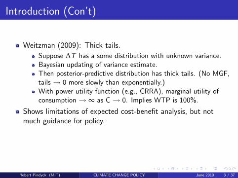
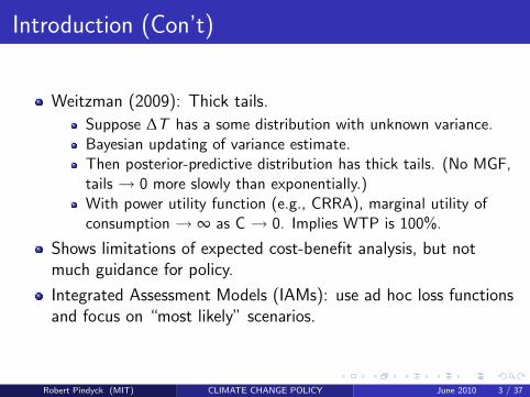
Weitzman (2009): Thick tails.
Suppose ∆T has a some distribution with unknown variance.Bayesian updating of variance estimate.Then posterior-predictive distribution has thick tails. (No MGF,tails → 0 more slowly than exponentially.)With power utility function (e.g., CRRA), marginal utility ofconsumption → ∞ as C → 0. Implies WTP is 100%.
Shows limitations of expected cost-benefit analysis, but notmuch guidance for policy.
Integrated Assessment Models (IAMs): use ad hoc loss functionsand focus on “most likely” scenarios.
Robert Pindyck (MIT) CLIMATE CHANGE POLICY June 2010 3 / 37

Introduction (Con’t)
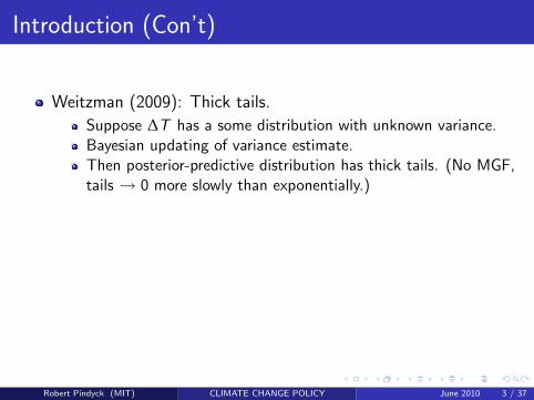
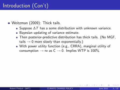
Weitzman (2009): Thick tails.
Suppose ∆T has a some distribution with unknown variance.
Bayesian updating of variance estimate.Then posterior-predictive distribution has thick tails. (No MGF,tails → 0 more slowly than exponentially.)With power utility function (e.g., CRRA), marginal utility ofconsumption → ∞ as C → 0. Implies WTP is 100%.
Shows limitations of expected cost-benefit analysis, but notmuch guidance for policy.
Integrated Assessment Models (IAMs): use ad hoc loss functionsand focus on “most likely” scenarios.
Robert Pindyck (MIT) CLIMATE CHANGE POLICY June 2010 3 / 37

Introduction (Con’t)
Weitzman (2009): Thick tails.
Suppose ∆T has a some distribution with unknown variance.Bayesian updating of variance estimate.
Then posterior-predictive distribution has thick tails. (No MGF,tails → 0 more slowly than exponentially.)With power utility function (e.g., CRRA), marginal utility ofconsumption → ∞ as C → 0. Implies WTP is 100%.
Shows limitations of expected cost-benefit analysis, but notmuch guidance for policy.
Integrated Assessment Models (IAMs): use ad hoc loss functionsand focus on “most likely” scenarios.
Robert Pindyck (MIT) CLIMATE CHANGE POLICY June 2010 3 / 37
Introduction (Con’t)
Weitzman (2009): Thick tails.
Suppose ∆T has a some distribution with unknown variance.Bayesian updating of variance estimate.Then posterior-predictive distribution has thick tails. (No MGF,tails → 0 more slowly than exponentially.)
With power utility function (e.g., CRRA), marginal utility ofconsumption → ∞ as C → 0. Implies WTP is 100%.
Shows limitations of expected cost-benefit analysis, but notmuch guidance for policy.
Integrated Assessment Models (IAMs): use ad hoc loss functionsand focus on “most likely” scenarios.
Robert Pindyck (MIT) CLIMATE CHANGE POLICY June 2010 3 / 37
Introduction (Con’t)
Weitzman (2009): Thick tails.
Suppose ∆T has a some distribution with unknown variance.Bayesian updating of variance estimate.Then posterior-predictive distribution has thick tails. (No MGF,tails → 0 more slowly than exponentially.)With power utility function (e.g., CRRA), marginal utility ofconsumption → ∞ as C → 0. Implies WTP is 100%.
Shows limitations of expected cost-benefit analysis, but notmuch guidance for policy.
Integrated Assessment Models (IAMs): use ad hoc loss functionsand focus on “most likely” scenarios.
Robert Pindyck (MIT) CLIMATE CHANGE POLICY June 2010 3 / 37

This Study
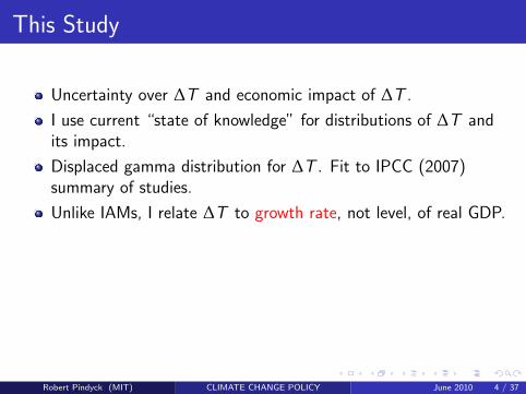
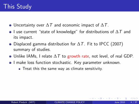
Uncertainty over ∆T and economic impact of ∆T .
I use current “state of knowledge” for distributions of ∆T andits impact.
Displaced gamma distribution for ∆T . Fit to IPCC (2007)summary of studies.
Unlike IAMs, I relate ∆T to growth rate, not level, of real GDP.
I make loss function stochastic. Key parameter unknown.
Treat this the same way as climate sensitivity.As with ∆T , displaced gamma distribution. Use recenteconomic impact studies (IAMs) to calibrate.
I ignore irreversibilities. Companion study.
Robert Pindyck (MIT) CLIMATE CHANGE POLICY June 2010 4 / 37
This Study
Uncertainty over ∆T and economic impact of ∆T .
I use current “state of knowledge” for distributions of ∆T andits impact.
Displaced gamma distribution for ∆T . Fit to IPCC (2007)summary of studies.
Unlike IAMs, I relate ∆T to growth rate, not level, of real GDP.
I make loss function stochastic. Key parameter unknown.
Treat this the same way as climate sensitivity.As with ∆T , displaced gamma distribution. Use recenteconomic impact studies (IAMs) to calibrate.
I ignore irreversibilities. Companion study.
Robert Pindyck (MIT) CLIMATE CHANGE POLICY June 2010 4 / 37
This Study
Uncertainty over ∆T and economic impact of ∆T .
I use current “state of knowledge” for distributions of ∆T andits impact.
Displaced gamma distribution for ∆T . Fit to IPCC (2007)summary of studies.
Unlike IAMs, I relate ∆T to growth rate, not level, of real GDP.
I make loss function stochastic. Key parameter unknown.
Treat this the same way as climate sensitivity.
As with ∆T , displaced gamma distribution. Use recenteconomic impact studies (IAMs) to calibrate.
I ignore irreversibilities. Companion study.
Robert Pindyck (MIT) CLIMATE CHANGE POLICY June 2010 4 / 37

This Study
Uncertainty over ∆T and economic impact of ∆T .
I use current “state of knowledge” for distributions of ∆T andits impact.
Displaced gamma distribution for ∆T . Fit to IPCC (2007)summary of studies.
Unlike IAMs, I relate ∆T to growth rate, not level, of real GDP.
I make loss function stochastic. Key parameter unknown.
Treat this the same way as climate sensitivity.As with ∆T , displaced gamma distribution. Use recenteconomic impact studies (IAMs) to calibrate.
I ignore irreversibilities. Companion study.
Robert Pindyck (MIT) CLIMATE CHANGE POLICY June 2010 4 / 37

Plan for Talk
Background and overview of methodology.
Uncertainty over climate sensitivity, use of gamma distribution.
Economic impact of ∆T .
Choice of loss function.Treatment of uncertainty.
Willingness to pay to keep (uncertain) ∆T ≤ τ.
General formulation.No uncertainty.Only uncertainty over ∆T .
Policy implications and conclusions.
Robert Pindyck (MIT) CLIMATE CHANGE POLICY June 2010 5 / 37
Standard IAM Policy Analysis
Economic analyses usually built around 5 elements:
1 Project future emissions (of CO2e composite or individualGHGs) under BAU and abatement scenarios, and resultingatmospheric CO2e.
2 Project resulting ∆T over time (globally or regionally).3 Translate ∆T into lost GDP and consumption (globally or
regionally). This is most speculative part, because hard toestimate potential adaptation.
4 Estimate current and future costs of abating GHG emissions byvarious amounts.
5 Assumptions about social utility, pure rate of time preference,and but-for growth, for intertemporal comparisons.
For each step, substantial uncertainty.
Robert Pindyck (MIT) CLIMATE CHANGE POLICY June 2010 6 / 37
Standard IAM Policy Analysis
Economic analyses usually built around 5 elements:1 Project future emissions (of CO2e composite or individual
GHGs) under BAU and abatement scenarios, and resultingatmospheric CO2e.
2 Project resulting ∆T over time (globally or regionally).
3 Translate ∆T into lost GDP and consumption (globally orregionally). This is most speculative part, because hard toestimate potential adaptation.
4 Estimate current and future costs of abating GHG emissions byvarious amounts.
5 Assumptions about social utility, pure rate of time preference,and but-for growth, for intertemporal comparisons.
For each step, substantial uncertainty.
Robert Pindyck (MIT) CLIMATE CHANGE POLICY June 2010 6 / 37
Standard IAM Policy Analysis
Economic analyses usually built around 5 elements:1 Project future emissions (of CO2e composite or individual
GHGs) under BAU and abatement scenarios, and resultingatmospheric CO2e.
2 Project resulting ∆T over time (globally or regionally).3 Translate ∆T into lost GDP and consumption (globally or
regionally). This is most speculative part, because hard toestimate potential adaptation.
4 Estimate current and future costs of abating GHG emissions byvarious amounts.
5 Assumptions about social utility, pure rate of time preference,and but-for growth, for intertemporal comparisons.
For each step, substantial uncertainty.
Robert Pindyck (MIT) CLIMATE CHANGE POLICY June 2010 6 / 37
Standard IAM Policy Analysis
Economic analyses usually built around 5 elements:1 Project future emissions (of CO2e composite or individual
GHGs) under BAU and abatement scenarios, and resultingatmospheric CO2e.
2 Project resulting ∆T over time (globally or regionally).3 Translate ∆T into lost GDP and consumption (globally or
regionally). This is most speculative part, because hard toestimate potential adaptation.
4 Estimate current and future costs of abating GHG emissions byvarious amounts.
5 Assumptions about social utility, pure rate of time preference,and but-for growth, for intertemporal comparisons.
For each step, substantial uncertainty.
Robert Pindyck (MIT) CLIMATE CHANGE POLICY June 2010 6 / 37
IAM Analyses (Con’t)
Apart from Stern Review (low discount rate, low abatementcosts, high economic impact), most studies suggest low tomoderate abatement now (or waiting).
Increasing rate of abatement is dynamically efficient, allows forlearning about ∆T and its impact, and allows for technologicalchange (e.g., lower abatement costs).
If you believe ∆T is within IPCC’s 90% confidence interval, hardto justify stringent abatement now.
Maybe not: Might tails of the distributions for ∆T and/orimpact — possibility of extreme outcomes — support stringentabatement?
Robert Pindyck (MIT) CLIMATE CHANGE POLICY June 2010 7 / 37
Methodology
I avoid dealing with abatement costs and GHG emissions andaccumulation by estimating WTP, and focusing on uncertaintyover ∆T and economic impact.
Temperature Change. Use IPCC survey of 22 studies of climatesensitivity.
Fit displaced gamma distribution for ∆TH , H = 100 years.Studies too “conservative?” Can re-fit to subset with largertails; can change variance or skewness of base distribution.I assume immediate doubling of GHG concentration,∆Tt → 2∆TH as t gets large:
∆Tt = 2∆TH [1− (1/ 2)t/ H ]
Robert Pindyck (MIT) CLIMATE CHANGE POLICY June 2010 8 / 37

Methodology
I avoid dealing with abatement costs and GHG emissions andaccumulation by estimating WTP, and focusing on uncertaintyover ∆T and economic impact.
Temperature Change. Use IPCC survey of 22 studies of climatesensitivity.
Fit displaced gamma distribution for ∆TH , H = 100 years.
Studies too “conservative?” Can re-fit to subset with largertails; can change variance or skewness of base distribution.I assume immediate doubling of GHG concentration,∆Tt → 2∆TH as t gets large:
∆Tt = 2∆TH [1− (1/ 2)t/ H ]
Robert Pindyck (MIT) CLIMATE CHANGE POLICY June 2010 8 / 37

Methodology
I avoid dealing with abatement costs and GHG emissions andaccumulation by estimating WTP, and focusing on uncertaintyover ∆T and economic impact.
Temperature Change. Use IPCC survey of 22 studies of climatesensitivity.
Fit displaced gamma distribution for ∆TH , H = 100 years.Studies too “conservative?” Can re-fit to subset with largertails; can change variance or skewness of base distribution.
I assume immediate doubling of GHG concentration,∆Tt → 2∆TH as t gets large:
∆Tt = 2∆TH [1− (1/ 2)t/ H ]
Robert Pindyck (MIT) CLIMATE CHANGE POLICY June 2010 8 / 37

Methodology
I avoid dealing with abatement costs and GHG emissions andaccumulation by estimating WTP, and focusing on uncertaintyover ∆T and economic impact.
Temperature Change. Use IPCC survey of 22 studies of climatesensitivity.
Fit displaced gamma distribution for ∆TH , H = 100 years.Studies too “conservative?” Can re-fit to subset with largertails; can change variance or skewness of base distribution.I assume immediate doubling of GHG concentration,∆Tt → 2∆TH as t gets large:
∆Tt = 2∆TH [1− (1/ 2)t/ H ]
Robert Pindyck (MIT) CLIMATE CHANGE POLICY June 2010 8 / 37

Methodology (Con’t)
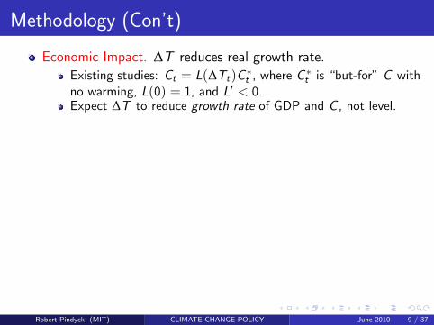
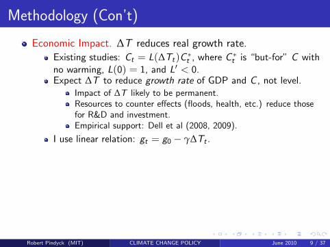
Economic Impact. ∆T reduces real growth rate.
Existing studies: Ct = L(∆Tt)C ∗t , where C ∗
t is “but-for” C withno warming, L(0) = 1, and L′ < 0.Expect ∆T to reduce growth rate of GDP and C , not level.
Impact of ∆T likely to be permanent.Resources to counter effects (floods, health, etc.) reduce thosefor R&D and investment.Empirical support: Dell et al (2008, 2009).
I use linear relation: gt = g0 − γ∆Tt .Use IAMs to get dist. for β in L(∆T ) = e−β(∆T )2 at H = 100.Translate into distribution for γ. Normalizing C0 = 1,
Ct = e∫ t0 g (s)ds = e
− 2γH∆THln(1/ 2) +(g0−2γ∆TH )t+ 2γH∆TH
ln(1/ 2) (1/ 2)t/ H
Then e− 2γH∆TH
ln(1/ 2) +(g0−2γ∆TH )H+ γH∆THln(1/ 2) = eg0H−β(∆T )2 , and
γ = 1.79β∆TH / H.
Robert Pindyck (MIT) CLIMATE CHANGE POLICY June 2010 9 / 37

Methodology (Con’t)
Economic Impact. ∆T reduces real growth rate.Existing studies: Ct = L(∆Tt)C ∗
t , where C ∗t is “but-for” C with
no warming, L(0) = 1, and L′ < 0.
Expect ∆T to reduce growth rate of GDP and C , not level.
Impact of ∆T likely to be permanent.Resources to counter effects (floods, health, etc.) reduce thosefor R&D and investment.Empirical support: Dell et al (2008, 2009).
I use linear relation: gt = g0 − γ∆Tt .Use IAMs to get dist. for β in L(∆T ) = e−β(∆T )2 at H = 100.Translate into distribution for γ. Normalizing C0 = 1,
Ct = e∫ t0 g (s)ds = e
− 2γH∆THln(1/ 2) +(g0−2γ∆TH )t+ 2γH∆TH
ln(1/ 2) (1/ 2)t/ H
Then e− 2γH∆TH
ln(1/ 2) +(g0−2γ∆TH )H+ γH∆THln(1/ 2) = eg0H−β(∆T )2 , and
γ = 1.79β∆TH / H.
Robert Pindyck (MIT) CLIMATE CHANGE POLICY June 2010 9 / 37
Methodology (Con’t)
Economic Impact. ∆T reduces real growth rate.Existing studies: Ct = L(∆Tt)C ∗
t , where C ∗t is “but-for” C with
no warming, L(0) = 1, and L′ < 0.Expect ∆T to reduce growth rate of GDP and C , not level.
Impact of ∆T likely to be permanent.Resources to counter effects (floods, health, etc.) reduce thosefor R&D and investment.Empirical support: Dell et al (2008, 2009).
I use linear relation: gt = g0 − γ∆Tt .Use IAMs to get dist. for β in L(∆T ) = e−β(∆T )2 at H = 100.Translate into distribution for γ. Normalizing C0 = 1,
Ct = e∫ t0 g (s)ds = e
− 2γH∆THln(1/ 2) +(g0−2γ∆TH )t+ 2γH∆TH
ln(1/ 2) (1/ 2)t/ H
Then e− 2γH∆TH
ln(1/ 2) +(g0−2γ∆TH )H+ γH∆THln(1/ 2) = eg0H−β(∆T )2 , and
γ = 1.79β∆TH / H.
Robert Pindyck (MIT) CLIMATE CHANGE POLICY June 2010 9 / 37

Methodology (Con’t)
Economic Impact. ∆T reduces real growth rate.Existing studies: Ct = L(∆Tt)C ∗
t , where C ∗t is “but-for” C with
no warming, L(0) = 1, and L′ < 0.Expect ∆T to reduce growth rate of GDP and C , not level.
Impact of ∆T likely to be permanent.
Resources to counter effects (floods, health, etc.) reduce thosefor R&D and investment.Empirical support: Dell et al (2008, 2009).
I use linear relation: gt = g0 − γ∆Tt .Use IAMs to get dist. for β in L(∆T ) = e−β(∆T )2 at H = 100.Translate into distribution for γ. Normalizing C0 = 1,
Ct = e∫ t0 g (s)ds = e
− 2γH∆THln(1/ 2) +(g0−2γ∆TH )t+ 2γH∆TH
ln(1/ 2) (1/ 2)t/ H
Then e− 2γH∆TH
ln(1/ 2) +(g0−2γ∆TH )H+ γH∆THln(1/ 2) = eg0H−β(∆T )2 , and
γ = 1.79β∆TH / H.
Robert Pindyck (MIT) CLIMATE CHANGE POLICY June 2010 9 / 37

Methodology (Con’t)
Economic Impact. ∆T reduces real growth rate.Existing studies: Ct = L(∆Tt)C ∗
t , where C ∗t is “but-for” C with
no warming, L(0) = 1, and L′ < 0.Expect ∆T to reduce growth rate of GDP and C , not level.
Impact of ∆T likely to be permanent.Resources to counter effects (floods, health, etc.) reduce thosefor R&D and investment.
Empirical support: Dell et al (2008, 2009).
I use linear relation: gt = g0 − γ∆Tt .Use IAMs to get dist. for β in L(∆T ) = e−β(∆T )2 at H = 100.Translate into distribution for γ. Normalizing C0 = 1,
Ct = e∫ t0 g (s)ds = e
− 2γH∆THln(1/ 2) +(g0−2γ∆TH )t+ 2γH∆TH
ln(1/ 2) (1/ 2)t/ H
Then e− 2γH∆TH
ln(1/ 2) +(g0−2γ∆TH )H+ γH∆THln(1/ 2) = eg0H−β(∆T )2 , and
γ = 1.79β∆TH / H.
Robert Pindyck (MIT) CLIMATE CHANGE POLICY June 2010 9 / 37

Methodology (Con’t)
Economic Impact. ∆T reduces real growth rate.Existing studies: Ct = L(∆Tt)C ∗
t , where C ∗t is “but-for” C with
no warming, L(0) = 1, and L′ < 0.Expect ∆T to reduce growth rate of GDP and C , not level.
Impact of ∆T likely to be permanent.Resources to counter effects (floods, health, etc.) reduce thosefor R&D and investment.Empirical support: Dell et al (2008, 2009).
I use linear relation: gt = g0 − γ∆Tt .Use IAMs to get dist. for β in L(∆T ) = e−β(∆T )2 at H = 100.Translate into distribution for γ. Normalizing C0 = 1,
Ct = e∫ t0 g (s)ds = e
− 2γH∆THln(1/ 2) +(g0−2γ∆TH )t+ 2γH∆TH
ln(1/ 2) (1/ 2)t/ H
Then e− 2γH∆TH
ln(1/ 2) +(g0−2γ∆TH )H+ γH∆THln(1/ 2) = eg0H−β(∆T )2 , and
γ = 1.79β∆TH / H.
Robert Pindyck (MIT) CLIMATE CHANGE POLICY June 2010 9 / 37
Methodology (Con’t)
Economic Impact. ∆T reduces real growth rate.Existing studies: Ct = L(∆Tt)C ∗
t , where C ∗t is “but-for” C with
no warming, L(0) = 1, and L′ < 0.Expect ∆T to reduce growth rate of GDP and C , not level.
Impact of ∆T likely to be permanent.Resources to counter effects (floods, health, etc.) reduce thosefor R&D and investment.Empirical support: Dell et al (2008, 2009).
I use linear relation: gt = g0 − γ∆Tt .
Use IAMs to get dist. for β in L(∆T ) = e−β(∆T )2 at H = 100.Translate into distribution for γ. Normalizing C0 = 1,
Ct = e∫ t0 g (s)ds = e
− 2γH∆THln(1/ 2) +(g0−2γ∆TH )t+ 2γH∆TH
ln(1/ 2) (1/ 2)t/ H
Then e− 2γH∆TH
ln(1/ 2) +(g0−2γ∆TH )H+ γH∆THln(1/ 2) = eg0H−β(∆T )2 , and
γ = 1.79β∆TH / H.
Robert Pindyck (MIT) CLIMATE CHANGE POLICY June 2010 9 / 37

Methodology (Con’t)
Economic Impact. ∆T reduces real growth rate.Existing studies: Ct = L(∆Tt)C ∗
t , where C ∗t is “but-for” C with
no warming, L(0) = 1, and L′ < 0.Expect ∆T to reduce growth rate of GDP and C , not level.
Impact of ∆T likely to be permanent.Resources to counter effects (floods, health, etc.) reduce thosefor R&D and investment.Empirical support: Dell et al (2008, 2009).
I use linear relation: gt = g0 − γ∆Tt .Use IAMs to get dist. for β in L(∆T ) = e−β(∆T )2 at H = 100.
Translate into distribution for γ. Normalizing C0 = 1,
Ct = e∫ t0 g (s)ds = e
− 2γH∆THln(1/ 2) +(g0−2γ∆TH )t+ 2γH∆TH
ln(1/ 2) (1/ 2)t/ H
Then e− 2γH∆TH
ln(1/ 2) +(g0−2γ∆TH )H+ γH∆THln(1/ 2) = eg0H−β(∆T )2 , and
γ = 1.79β∆TH / H.
Robert Pindyck (MIT) CLIMATE CHANGE POLICY June 2010 9 / 37

Methodology (Con’t)
Economic Impact. ∆T reduces real growth rate.Existing studies: Ct = L(∆Tt)C ∗
t , where C ∗t is “but-for” C with
no warming, L(0) = 1, and L′ < 0.Expect ∆T to reduce growth rate of GDP and C , not level.
Impact of ∆T likely to be permanent.Resources to counter effects (floods, health, etc.) reduce thosefor R&D and investment.Empirical support: Dell et al (2008, 2009).
I use linear relation: gt = g0 − γ∆Tt .Use IAMs to get dist. for β in L(∆T ) = e−β(∆T )2 at H = 100.Translate into distribution for γ. Normalizing C0 = 1,
Ct = e∫ t0 g (s)ds = e
− 2γH∆THln(1/ 2) +(g0−2γ∆TH )t+ 2γH∆TH
ln(1/ 2) (1/ 2)t/ H
Then e− 2γH∆TH
ln(1/ 2) +(g0−2γ∆TH )H+ γH∆THln(1/ 2) = eg0H−β(∆T )2 , and
γ = 1.79β∆TH / H.
Robert Pindyck (MIT) CLIMATE CHANGE POLICY June 2010 9 / 37
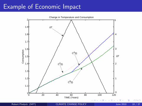
Example of Economic Impact
0 20 40 60 80 100 1201
1.1
1.2
1.3
1.4
1.5
1.6
1.7
1.8
1.9
2Change in Temperature and Consumption
TIME (Years)
Con
sum
ptio
n
0
1
2
3
4
5
∆T
C0(t)
CB(t)
CA(t)∆T
Robert Pindyck (MIT) CLIMATE CHANGE POLICY June 2010 10 / 37

Willingness to Pay
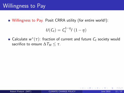
Willingness to Pay. Posit CRRA utility (for entire world!):
U(Ct) = C1−ηt / (1− η)
Calculate w ∗(τ): fraction of current and future Ct society wouldsacrifice to ensure ∆TH ≤ τ.If we sacrifice w(τ) of {Ct} so ∆TH ≤ τ, welfare is:
W1(τ) =[1− w(τ)]1−η
1− ηE0,τ
∫ ∞
0eω−ρt−ω(1/ 2)t/ H
dt
where ρ = (η − 1)(g0 − 2γ∆TH) + δ,ω = 2(η − 1)γH∆TH / ln(1/ 2), and E0,τ is expectation over∆TH and γ conditional on ∆TH ≤ τ.
Robert Pindyck (MIT) CLIMATE CHANGE POLICY June 2010 11 / 37
Willingness to Pay
Willingness to Pay. Posit CRRA utility (for entire world!):
U(Ct) = C1−ηt / (1− η)
Calculate w ∗(τ): fraction of current and future Ct society wouldsacrifice to ensure ∆TH ≤ τ.
If we sacrifice w(τ) of {Ct} so ∆TH ≤ τ, welfare is:
W1(τ) =[1− w(τ)]1−η
1− ηE0,τ
∫ ∞
0eω−ρt−ω(1/ 2)t/ H
dt
where ρ = (η − 1)(g0 − 2γ∆TH) + δ,ω = 2(η − 1)γH∆TH / ln(1/ 2), and E0,τ is expectation over∆TH and γ conditional on ∆TH ≤ τ.
Robert Pindyck (MIT) CLIMATE CHANGE POLICY June 2010 11 / 37

Willingness to Pay
Willingness to Pay. Posit CRRA utility (for entire world!):
U(Ct) = C1−ηt / (1− η)
Calculate w ∗(τ): fraction of current and future Ct society wouldsacrifice to ensure ∆TH ≤ τ.If we sacrifice w(τ) of {Ct} so ∆TH ≤ τ, welfare is:
W1(τ) =[1− w(τ)]1−η
1− ηE0,τ
∫ ∞
0eω−ρt−ω(1/ 2)t/ H
dt
where ρ = (η − 1)(g0 − 2γ∆TH) + δ,ω = 2(η − 1)γH∆TH / ln(1/ 2), and E0,τ is expectation over∆TH and γ conditional on ∆TH ≤ τ.
Robert Pindyck (MIT) CLIMATE CHANGE POLICY June 2010 11 / 37

Willingness to Pay (Con’t)
If no action is taken, welfare is:
W2 =1
1− ηE0
∫ ∞
0eω−ρt−ω(1/ 2)t/ H
dt
where E0 is expectation with ∆TH unconstrained.
WTP is value w ∗(τ) that equates W1(τ) and W2.
Question: Do fitted distributions for ∆TH and γ, along with“reasonable” values for δ, η and g0, yield w ∗(τ) > 2 or 3% forτ around 2 or 3◦C?
Robert Pindyck (MIT) CLIMATE CHANGE POLICY June 2010 12 / 37

Distribution for ∆T
Fit a displaced gamma distribution:
f (x ; r , λ, θ) =λr
Γ(r)(x − θ)2e−λ(x−θ) , x ≥ θ
where Γ(r) is Gamma function:
Γ(r) =∫ ∞
0sr−1e−sds
Here θ is the displacement parameter. Moment generatingfunction is
Mx (t) = E(etx ) =(
λ
λ− t
)r
etθ
Robert Pindyck (MIT) CLIMATE CHANGE POLICY June 2010 13 / 37

Distribution for ∆T (Con’t)
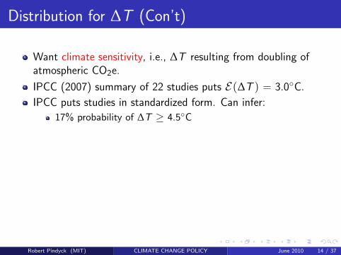
Want climate sensitivity, i.e., ∆T resulting from doubling ofatmospheric CO2e.
IPCC (2007) summary of 22 studies puts E(∆T ) = 3.0◦C.
IPCC puts studies in standardized form. Can infer:
17% probability of ∆T ≥ 4.5◦C5% probability of ∆T ≥ 7.0◦C1% probability of ∆T ≥ 10.0◦C
Fitting distribution to mean, 5%, and 1% points gives r = 3.8,λ = 0.92, and θ = −1.13.
Implies 21% probability of ∆T ≥ 4.5◦C.
Implies 2.9% probability of negative ∆T , consistent withscientific studies.
Robert Pindyck (MIT) CLIMATE CHANGE POLICY June 2010 14 / 37

Distribution for ∆T (Con’t)
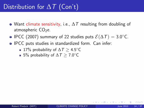
Want climate sensitivity, i.e., ∆T resulting from doubling ofatmospheric CO2e.
IPCC (2007) summary of 22 studies puts E(∆T ) = 3.0◦C.
IPCC puts studies in standardized form. Can infer:
17% probability of ∆T ≥ 4.5◦C5% probability of ∆T ≥ 7.0◦C1% probability of ∆T ≥ 10.0◦C
Fitting distribution to mean, 5%, and 1% points gives r = 3.8,λ = 0.92, and θ = −1.13.
Implies 21% probability of ∆T ≥ 4.5◦C.
Implies 2.9% probability of negative ∆T , consistent withscientific studies.
Robert Pindyck (MIT) CLIMATE CHANGE POLICY June 2010 14 / 37

Distribution for ∆T (Con’t)
Want climate sensitivity, i.e., ∆T resulting from doubling ofatmospheric CO2e.
IPCC (2007) summary of 22 studies puts E(∆T ) = 3.0◦C.
IPCC puts studies in standardized form. Can infer:
17% probability of ∆T ≥ 4.5◦C5% probability of ∆T ≥ 7.0◦C1% probability of ∆T ≥ 10.0◦C
Fitting distribution to mean, 5%, and 1% points gives r = 3.8,λ = 0.92, and θ = −1.13.
Implies 21% probability of ∆T ≥ 4.5◦C.
Implies 2.9% probability of negative ∆T , consistent withscientific studies.
Robert Pindyck (MIT) CLIMATE CHANGE POLICY June 2010 14 / 37
Distribution for ∆T (Con’t)
Want climate sensitivity, i.e., ∆T resulting from doubling ofatmospheric CO2e.
IPCC (2007) summary of 22 studies puts E(∆T ) = 3.0◦C.
IPCC puts studies in standardized form. Can infer:
17% probability of ∆T ≥ 4.5◦C
5% probability of ∆T ≥ 7.0◦C1% probability of ∆T ≥ 10.0◦C
Fitting distribution to mean, 5%, and 1% points gives r = 3.8,λ = 0.92, and θ = −1.13.
Implies 21% probability of ∆T ≥ 4.5◦C.
Implies 2.9% probability of negative ∆T , consistent withscientific studies.
Robert Pindyck (MIT) CLIMATE CHANGE POLICY June 2010 14 / 37
Distribution for ∆T (Con’t)
Want climate sensitivity, i.e., ∆T resulting from doubling ofatmospheric CO2e.
IPCC (2007) summary of 22 studies puts E(∆T ) = 3.0◦C.
IPCC puts studies in standardized form. Can infer:
17% probability of ∆T ≥ 4.5◦C5% probability of ∆T ≥ 7.0◦C
1% probability of ∆T ≥ 10.0◦C
Fitting distribution to mean, 5%, and 1% points gives r = 3.8,λ = 0.92, and θ = −1.13.
Implies 21% probability of ∆T ≥ 4.5◦C.
Implies 2.9% probability of negative ∆T , consistent withscientific studies.
Robert Pindyck (MIT) CLIMATE CHANGE POLICY June 2010 14 / 37

Distribution for ∆T (Con’t)
Want climate sensitivity, i.e., ∆T resulting from doubling ofatmospheric CO2e.
IPCC (2007) summary of 22 studies puts E(∆T ) = 3.0◦C.
IPCC puts studies in standardized form. Can infer:
17% probability of ∆T ≥ 4.5◦C5% probability of ∆T ≥ 7.0◦C1% probability of ∆T ≥ 10.0◦C
Fitting distribution to mean, 5%, and 1% points gives r = 3.8,λ = 0.92, and θ = −1.13.
Implies 21% probability of ∆T ≥ 4.5◦C.
Implies 2.9% probability of negative ∆T , consistent withscientific studies.
Robert Pindyck (MIT) CLIMATE CHANGE POLICY June 2010 14 / 37

Fitted Distribution for ∆TH
−2 0 2 3 4.5 6 7 8 10 12 140
0.05
0.1
0.15
0.2
0.25
Climate Sensitivity DistributionMean = 3.0, λ = 0.92, r = 3.8
Temperature Change, ∆ T
f(∆ T
)
.029
θ = −1.13
Robert Pindyck (MIT) CLIMATE CHANGE POLICY June 2010 15 / 37

∆Tt : Unconstrained and Constrained so ∆TH ≤ τ
Recall ∆Tt = 2∆TH [1− (1/ 2)t / H ].
0 20 40 60 80 100 120 140 160 180 2000
1
2
3
4
5
6
7
8
Change in Temperature: Unconstrained and Constrained to ∆TH≤τ
TIME (Years)
∆T
∆TH
∆T(τ=0)
∆TH(τ)
∆T(τ=3)
∆T
Robert Pindyck (MIT) CLIMATE CHANGE POLICY June 2010 16 / 37
Uncertainty Over Economic Impact
How bad would be a ∆T ≥ 5◦C?
Might argue we do not — and cannot — know. Outside of ourexperience and models.
Could say same thing about probabilities of ∆T beyond 5◦C;outside of experience and range of climate science models.
Alternative: treat IAMs and related models analogously toclimate science models.
IAMs give range (and confidence points) of lost GDP for 4◦Cand 5◦C ∆T .
Can use this information to get probability distribution foreconomic impact.
Robert Pindyck (MIT) CLIMATE CHANGE POLICY June 2010 17 / 37

Economic Impact
Begin with exponential-quadratic: L(∆T ) = exp[−β(∆T )2]
Treat β as stochastic.
DG distribution, g(β); β and ∆T independently distributed.
Calibrate parameters of distribution for β using:
IPCC (2007) — for ∆T = 4◦C, global mean loss “ most likely”in range of 1% to 5% of GDP.
“Most likely” = 66% to 90% confidence interval.
Dietz and Stern (2008) graphical summary of IAM damageestimates shows 0.5% to 2% of lost GDP for ∆T = 3◦C, and1% to 8% of GDP for ∆T = 5◦C.
Robert Pindyck (MIT) CLIMATE CHANGE POLICY June 2010 18 / 37

Economic Impact
Begin with exponential-quadratic: L(∆T ) = exp[−β(∆T )2]Treat β as stochastic.
DG distribution, g(β); β and ∆T independently distributed.
Calibrate parameters of distribution for β using:
IPCC (2007) — for ∆T = 4◦C, global mean loss “ most likely”in range of 1% to 5% of GDP.
“Most likely” = 66% to 90% confidence interval.
Dietz and Stern (2008) graphical summary of IAM damageestimates shows 0.5% to 2% of lost GDP for ∆T = 3◦C, and1% to 8% of GDP for ∆T = 5◦C.
Robert Pindyck (MIT) CLIMATE CHANGE POLICY June 2010 18 / 37
Economic Impact (Con’t)
Want distribution for γ in gt = g0 − γ∆Tt . Useγ = 1.79β∆T / H .
Using IPCC range, I take mean loss for ∆T = 4◦C to be 3% ofGDP, and 5% and 95% points (or 17% and 83% points) to be1% of GDP and 5% of GDP. Results consistent with summarynumbers in Dietz and Stern.
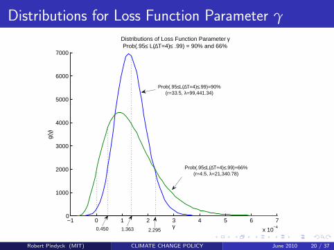
Implies that mean, 5% and 95% (or 17% and 83%) values for γare γ0 = .0001363, γ1 = .0000450, and γ2 = .0002295.
I fit DGD to these numbers, and use higher-variance version forWTP calculations.
Robert Pindyck (MIT) CLIMATE CHANGE POLICY June 2010 19 / 37

Economic Impact (Con’t)
Want distribution for γ in gt = g0 − γ∆Tt . Useγ = 1.79β∆T / H .
Using IPCC range, I take mean loss for ∆T = 4◦C to be 3% ofGDP, and 5% and 95% points (or 17% and 83% points) to be1% of GDP and 5% of GDP. Results consistent with summarynumbers in Dietz and Stern.
Implies that mean, 5% and 95% (or 17% and 83%) values for γare γ0 = .0001363, γ1 = .0000450, and γ2 = .0002295.
I fit DGD to these numbers, and use higher-variance version forWTP calculations.
Robert Pindyck (MIT) CLIMATE CHANGE POLICY June 2010 19 / 37
Distributions for Loss Function Parameter γ
−1 0 1 2 3 4 5 6 7
x 10−4
0
1000
2000
3000
4000
5000
6000
7000
Distributions of Loss Function Parameter γProb(.95≤ L(∆T=4)≤ .99) = 90% and 66%
γ
g(γ)
Prob(.95≤L(∆T=4)≤.99)=90%(r=33.5, λ=99,441.34)
Prob(.95≤L(∆T=4)≤.99)=66%(r=4.5, λ=21,340.78)
0.450 1.363 2.295
Robert Pindyck (MIT) CLIMATE CHANGE POLICY June 2010 20 / 37

Willingness to Pay
Given distributions f (∆T ) and g(γ), denote by Mτ(t) andM∞(t) the time-t expectations:
Mτ(t) =1
F (τ)
∫ τ
θT
∫ ∞
θγ
eω−ρt−ω(1/ 2)t/ Hf (∆T )g(γ)d∆Tdγ
M∞(t) =∫ ∞
θT
∫ ∞
θγ
eω−ρt−ω(1/ 2)t/ Hf (∆T )g(γ)d∆Tdγ
where θT and θγ are lower limits on distributions for ∆T and γ,
and F (τ) =∫ τ
θTf (∆T )d∆T .
Thus W1(τ) (abatement) and W2 (no abatement) are:
W1(τ) =[1− w(τ)]1−η
1− η
∫ ∞
0Mτ(t)dt ≡ [1− w(τ)]1−η
1− ηGτ
W2 =1
1− η
∫ ∞
0M∞(t)dt ≡ 1
1− ηG∞
Robert Pindyck (MIT) CLIMATE CHANGE POLICY June 2010 21 / 37

Willingness to Pay (Con’t)
Setting W1(τ) = W2, WTP is
w ∗(τ) = 1 − [G∞/ Gτ]1
1−η
Parameter Values. Want “reasonable” numbers for δ, η, and g0,but skewed to high WTP.
Translation: want “small” δ, η, and g0.
In finance and macro literature, δ usually .01 to .04.Can argue (value judgment) for intergenerational comparisons,δ should be close to 0.In finance and macro literature, η usually 1.5 to 4.Actual g0 around .02 to .025.
I will use δ = 0, η ≈ 2, and g0 from .015 to .025.
Robert Pindyck (MIT) CLIMATE CHANGE POLICY June 2010 22 / 37

Willingness to Pay (Con’t)
Setting W1(τ) = W2, WTP is
w ∗(τ) = 1 − [G∞/ Gτ]1
1−η
Parameter Values. Want “reasonable” numbers for δ, η, and g0,but skewed to high WTP.
Translation: want “small” δ, η, and g0.
In finance and macro literature, δ usually .01 to .04.
Can argue (value judgment) for intergenerational comparisons,δ should be close to 0.In finance and macro literature, η usually 1.5 to 4.Actual g0 around .02 to .025.
I will use δ = 0, η ≈ 2, and g0 from .015 to .025.
Robert Pindyck (MIT) CLIMATE CHANGE POLICY June 2010 22 / 37

Willingness to Pay (Con’t)
Setting W1(τ) = W2, WTP is
w ∗(τ) = 1 − [G∞/ Gτ]1
1−η
Parameter Values. Want “reasonable” numbers for δ, η, and g0,but skewed to high WTP.
Translation: want “small” δ, η, and g0.
In finance and macro literature, δ usually .01 to .04.Can argue (value judgment) for intergenerational comparisons,δ should be close to 0.
In finance and macro literature, η usually 1.5 to 4.Actual g0 around .02 to .025.
I will use δ = 0, η ≈ 2, and g0 from .015 to .025.
Robert Pindyck (MIT) CLIMATE CHANGE POLICY June 2010 22 / 37

Willingness to Pay (Con’t)
Setting W1(τ) = W2, WTP is
w ∗(τ) = 1 − [G∞/ Gτ]1
1−η
Parameter Values. Want “reasonable” numbers for δ, η, and g0,but skewed to high WTP.
Translation: want “small” δ, η, and g0.
In finance and macro literature, δ usually .01 to .04.Can argue (value judgment) for intergenerational comparisons,δ should be close to 0.In finance and macro literature, η usually 1.5 to 4.
Actual g0 around .02 to .025.
I will use δ = 0, η ≈ 2, and g0 from .015 to .025.
Robert Pindyck (MIT) CLIMATE CHANGE POLICY June 2010 22 / 37

Willingness to Pay (Con’t)
Setting W1(τ) = W2, WTP is
w ∗(τ) = 1 − [G∞/ Gτ]1
1−η
Parameter Values. Want “reasonable” numbers for δ, η, and g0,but skewed to high WTP.
Translation: want “small” δ, η, and g0.
In finance and macro literature, δ usually .01 to .04.Can argue (value judgment) for intergenerational comparisons,δ should be close to 0.In finance and macro literature, η usually 1.5 to 4.Actual g0 around .02 to .025.
I will use δ = 0, η ≈ 2, and g0 from .015 to .025.
Robert Pindyck (MIT) CLIMATE CHANGE POLICY June 2010 22 / 37

Willingness to Pay (Con’t)
Setting W1(τ) = W2, WTP is
w ∗(τ) = 1 − [G∞/ Gτ]1
1−η
Parameter Values. Want “reasonable” numbers for δ, η, and g0,but skewed to high WTP.
Translation: want “small” δ, η, and g0.
In finance and macro literature, δ usually .01 to .04.Can argue (value judgment) for intergenerational comparisons,δ should be close to 0.In finance and macro literature, η usually 1.5 to 4.Actual g0 around .02 to .025.
I will use δ = 0, η ≈ 2, and g0 from .015 to .025.
Robert Pindyck (MIT) CLIMATE CHANGE POLICY June 2010 22 / 37

No Uncertainty
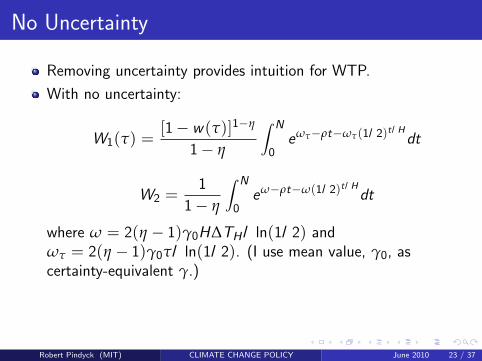
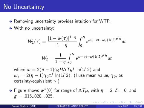
Removing uncertainty provides intuition for WTP.
With no uncertainty:
W1(τ) =[1− w(τ)]1−η
1− η
∫ N
0eωτ−ρt−ωτ(1/ 2)t/ H
dt
W2 =1
1− η
∫ N
0eω−ρt−ω(1/ 2)t/ H
dt
where ω = 2(η − 1)γ0H∆TH / ln(1/ 2) andωτ = 2(η − 1)γ0τ/ ln(1/ 2). (I use mean value, γ0, ascertainty-equivalent γ.)
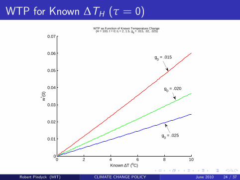
Figure shows w ∗(0) for range of ∆TH , with η = 2, δ = 0, andg = .015,.020, .025.
Robert Pindyck (MIT) CLIMATE CHANGE POLICY June 2010 23 / 37
No Uncertainty
Removing uncertainty provides intuition for WTP.
With no uncertainty:
W1(τ) =[1− w(τ)]1−η
1− η
∫ N
0eωτ−ρt−ωτ(1/ 2)t/ H
dt
W2 =1
1− η
∫ N
0eω−ρt−ω(1/ 2)t/ H
dt
where ω = 2(η − 1)γ0H∆TH / ln(1/ 2) andωτ = 2(η − 1)γ0τ/ ln(1/ 2). (I use mean value, γ0, ascertainty-equivalent γ.)
Figure shows w ∗(0) for range of ∆TH , with η = 2, δ = 0, andg = .015,.020, .025.
Robert Pindyck (MIT) CLIMATE CHANGE POLICY June 2010 23 / 37
WTP for Known ∆TH (τ = 0)
0 2 4 6 8 100
0.01
0.02
0.03
0.04
0.05
0.06
0.07
WTP as Function of Known Temperature Change(H = 100, τ = 0; η = 2, 1.5, g0 = .015, .02, .025)
Known ∆T (oC)
w* (0
)
g0 = .020
g0 = .025
g0 = .015
Robert Pindyck (MIT) CLIMATE CHANGE POLICY June 2010 24 / 37
Both ∆T and γ Uncertain
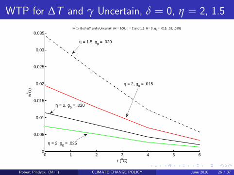
Both ∆T and the impact parameter γ are uncertain.
Figure shows w ∗(τ) for δ = 0, η = 2 and 1.5, and g0 = .015,.020, and .025.
To get WTP above 2%, even for τ = 0, need η = 1.5 org0 = .015 if η = 2.
Next figure shows w ∗(3) as function of η for g0 = .02. Forδ = 0, can get w ∗(3) > .05 if η close to 1.
If δ = .01, w ∗(3) < .02 for any η.
Robert Pindyck (MIT) CLIMATE CHANGE POLICY June 2010 25 / 37

Both ∆T and γ Uncertain
Both ∆T and the impact parameter γ are uncertain.
Figure shows w ∗(τ) for δ = 0, η = 2 and 1.5, and g0 = .015,.020, and .025.
To get WTP above 2%, even for τ = 0, need η = 1.5 org0 = .015 if η = 2.
Next figure shows w ∗(3) as function of η for g0 = .02. Forδ = 0, can get w ∗(3) > .05 if η close to 1.
If δ = .01, w ∗(3) < .02 for any η.
Robert Pindyck (MIT) CLIMATE CHANGE POLICY June 2010 25 / 37
WTP for ∆T and γ Uncertain, δ = 0, η = 2, 1.5
0 1 2 3 4 5 60
0.005
0.01
0.015
0.02
0.025
0.03
0.035w*(τ), Both ∆T and γ Uncertain (H = 100, η = 2 and 1.5, δ = 0, g0 = .015, .02, .025)
τ (oC)
w* (τ
)
η = 2, g0 = .015
η = 2, g0 = .020
η = 2, g0 = .025
η = 1.5, g0 = .020
Robert Pindyck (MIT) CLIMATE CHANGE POLICY June 2010 26 / 37

WTP Versus η for τ = 3.
1 1.5 2 2.5 3 3.5 40
0.01
0.02
0.03
0.04
0.05
0.06w*(3), Both ∆T and γ Uncertain, H = 100, g0 = .020, δ = 0 and .01)
η
w* (3
)
δ = 0
δ = .01
Robert Pindyck (MIT) CLIMATE CHANGE POLICY June 2010 27 / 37
Both ∆T and γ Uncertain (Con’t)
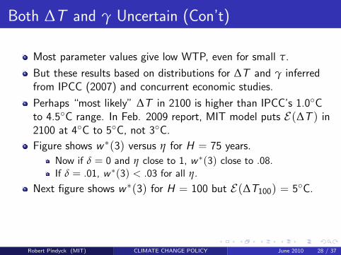
Most parameter values give low WTP, even for small τ.
But these results based on distributions for ∆T and γ inferredfrom IPCC (2007) and concurrent economic studies.
Perhaps “most likely” ∆T in 2100 is higher than IPCC’s 1.0◦Cto 4.5◦C range. In Feb. 2009 report, MIT model puts E(∆T ) in2100 at 4◦C to 5◦C, not 3◦C.
Figure shows w ∗(3) versus η for H = 75 years.
Now if δ = 0 and η close to 1, w ∗(3) close to .08.If δ = .01, w ∗(3) < .03 for all η.
Next figure shows w ∗(3) for H = 100 but E(∆T100) = 5◦C.
Now if η near 1, w ∗(3) close to 10%.But if δ = .01, w ∗(3) again very low for all η.
Robert Pindyck (MIT) CLIMATE CHANGE POLICY June 2010 28 / 37

Both ∆T and γ Uncertain (Con’t)
Most parameter values give low WTP, even for small τ.
But these results based on distributions for ∆T and γ inferredfrom IPCC (2007) and concurrent economic studies.
Perhaps “most likely” ∆T in 2100 is higher than IPCC’s 1.0◦Cto 4.5◦C range. In Feb. 2009 report, MIT model puts E(∆T ) in2100 at 4◦C to 5◦C, not 3◦C.
Figure shows w ∗(3) versus η for H = 75 years.
Now if δ = 0 and η close to 1, w ∗(3) close to .08.If δ = .01, w ∗(3) < .03 for all η.
Next figure shows w ∗(3) for H = 100 but E(∆T100) = 5◦C.
Now if η near 1, w ∗(3) close to 10%.But if δ = .01, w ∗(3) again very low for all η.
Robert Pindyck (MIT) CLIMATE CHANGE POLICY June 2010 28 / 37
Both ∆T and γ Uncertain (Con’t)
Most parameter values give low WTP, even for small τ.
But these results based on distributions for ∆T and γ inferredfrom IPCC (2007) and concurrent economic studies.
Perhaps “most likely” ∆T in 2100 is higher than IPCC’s 1.0◦Cto 4.5◦C range. In Feb. 2009 report, MIT model puts E(∆T ) in2100 at 4◦C to 5◦C, not 3◦C.
Figure shows w ∗(3) versus η for H = 75 years.
Now if δ = 0 and η close to 1, w ∗(3) close to .08.
If δ = .01, w ∗(3) < .03 for all η.
Next figure shows w ∗(3) for H = 100 but E(∆T100) = 5◦C.
Now if η near 1, w ∗(3) close to 10%.But if δ = .01, w ∗(3) again very low for all η.
Robert Pindyck (MIT) CLIMATE CHANGE POLICY June 2010 28 / 37

Both ∆T and γ Uncertain (Con’t)
Most parameter values give low WTP, even for small τ.
But these results based on distributions for ∆T and γ inferredfrom IPCC (2007) and concurrent economic studies.
Perhaps “most likely” ∆T in 2100 is higher than IPCC’s 1.0◦Cto 4.5◦C range. In Feb. 2009 report, MIT model puts E(∆T ) in2100 at 4◦C to 5◦C, not 3◦C.
Figure shows w ∗(3) versus η for H = 75 years.
Now if δ = 0 and η close to 1, w ∗(3) close to .08.If δ = .01, w ∗(3) < .03 for all η.
Next figure shows w ∗(3) for H = 100 but E(∆T100) = 5◦C.
Now if η near 1, w ∗(3) close to 10%.But if δ = .01, w ∗(3) again very low for all η.
Robert Pindyck (MIT) CLIMATE CHANGE POLICY June 2010 28 / 37
Both ∆T and γ Uncertain (Con’t)
Most parameter values give low WTP, even for small τ.
But these results based on distributions for ∆T and γ inferredfrom IPCC (2007) and concurrent economic studies.
Perhaps “most likely” ∆T in 2100 is higher than IPCC’s 1.0◦Cto 4.5◦C range. In Feb. 2009 report, MIT model puts E(∆T ) in2100 at 4◦C to 5◦C, not 3◦C.
Figure shows w ∗(3) versus η for H = 75 years.
Now if δ = 0 and η close to 1, w ∗(3) close to .08.If δ = .01, w ∗(3) < .03 for all η.
Next figure shows w ∗(3) for H = 100 but E(∆T100) = 5◦C.
Now if η near 1, w ∗(3) close to 10%.But if δ = .01, w ∗(3) again very low for all η.
Robert Pindyck (MIT) CLIMATE CHANGE POLICY June 2010 28 / 37

Both ∆T and γ Uncertain (Con’t)
Most parameter values give low WTP, even for small τ.
But these results based on distributions for ∆T and γ inferredfrom IPCC (2007) and concurrent economic studies.
Perhaps “most likely” ∆T in 2100 is higher than IPCC’s 1.0◦Cto 4.5◦C range. In Feb. 2009 report, MIT model puts E(∆T ) in2100 at 4◦C to 5◦C, not 3◦C.
Figure shows w ∗(3) versus η for H = 75 years.
Now if δ = 0 and η close to 1, w ∗(3) close to .08.If δ = .01, w ∗(3) < .03 for all η.
Next figure shows w ∗(3) for H = 100 but E(∆T100) = 5◦C.
Now if η near 1, w ∗(3) close to 10%.
But if δ = .01, w ∗(3) again very low for all η.
Robert Pindyck (MIT) CLIMATE CHANGE POLICY June 2010 28 / 37

Both ∆T and γ Uncertain (Con’t)
Most parameter values give low WTP, even for small τ.
But these results based on distributions for ∆T and γ inferredfrom IPCC (2007) and concurrent economic studies.
Perhaps “most likely” ∆T in 2100 is higher than IPCC’s 1.0◦Cto 4.5◦C range. In Feb. 2009 report, MIT model puts E(∆T ) in2100 at 4◦C to 5◦C, not 3◦C.
Figure shows w ∗(3) versus η for H = 75 years.
Now if δ = 0 and η close to 1, w ∗(3) close to .08.If δ = .01, w ∗(3) < .03 for all η.
Next figure shows w ∗(3) for H = 100 but E(∆T100) = 5◦C.
Now if η near 1, w ∗(3) close to 10%.But if δ = .01, w ∗(3) again very low for all η.
Robert Pindyck (MIT) CLIMATE CHANGE POLICY June 2010 28 / 37

WTP Versus η for τ = 3, H = 75 years.
1 1.5 2 2.5 3 3.5 40
0.01
0.02
0.03
0.04
0.05
0.06
0.07
0.08
0.09
w*(3), Both ∆T and γ Uncertain, H = 75, g
0 = .020, δ = 0 and .01)
η
w* (3
)
δ = .01
δ = 0
Robert Pindyck (MIT) CLIMATE CHANGE POLICY June 2010 29 / 37

WTP Versus η for τ = 3, E(∆T100) = 5◦C.
1 1.5 2 2.5 3 3.5 40
0.01
0.02
0.03
0.04
0.05
0.06
0.07
0.08
0.09
0.1w*(3), Both ∆T and γ Uncertain, (E(∆T) = 5, g0 = .020, δ = 0 and .01)
η
w* (3
)
δ = .01
δ = 0
Robert Pindyck (MIT) CLIMATE CHANGE POLICY June 2010 30 / 37

Policy Implications
Policy implications are rather stark.
For temperature and impact distributions based on IPCC and“conservative” parameter values (e.g., δ = 0, η = 2, g0 = .02),WTP to prevent any ∆T is around 2% or less.
If objective is to keep ∆T in 100 years below 3◦C (much morefeasible), WTP lower still.
Even if H = 75 or E(∆T ) = 5◦C, get high WTP only ifη < 1.5.
If δ = .01, get low WTP for all parameter combinations.
Robert Pindyck (MIT) CLIMATE CHANGE POLICY June 2010 31 / 37

Policy Implications (Con’t)
Two reasons. First, limited weight in tails of distributions for∆T and γ, consistent with studies surveyed by the IPCC.
Distribution for ∆T implies 21% probability of ∆T ≥ 4.5◦C in100 years, and 5% probability of ∆T ≥ 7.0◦C.
Distribution for γ implies a 17% probability of γ ≥ .00023.
∆T = 4.5◦C and γ = .00023 implies GDP in 100 years 5.7%lower than if ∆T = 0. But Prob(∆T ≥ 4.5◦C and γ ≥ .00023)only about 3.6%.
∆T = 7◦C (and γ = .00023) implies GDP in 100 years 9%lower, but probability only 0.9%.
Robert Pindyck (MIT) CLIMATE CHANGE POLICY June 2010 32 / 37

Policy Implications (Con’t)
Second, even with δ = 0, implicit discounting of consumption issignificant.
Initial consumption discount rate is ηg0, at least .03 if η = 2.And a (low-probability) 5.7 or 9 percent loss of GDP in 100years would involve much smaller losses in earlier years.
These results argue against stringent GHG abatement policy, butare consistent with moderate abatement.
2% of GDP in range of cost estimates for compliance withKyoto Protocol.
Taking U.S. in isolation, WTP of 2% implies $300 billion peryear for GHG abatement.
And if w ∗(3) = .01, would justify $150 billion per year ifabatement would limit ∆T to 3◦C.
Robert Pindyck (MIT) CLIMATE CHANGE POLICY June 2010 33 / 37

Policy Implications (Con’t)
Second, even with δ = 0, implicit discounting of consumption issignificant.
Initial consumption discount rate is ηg0, at least .03 if η = 2.
And a (low-probability) 5.7 or 9 percent loss of GDP in 100years would involve much smaller losses in earlier years.
These results argue against stringent GHG abatement policy, butare consistent with moderate abatement.
2% of GDP in range of cost estimates for compliance withKyoto Protocol.
Taking U.S. in isolation, WTP of 2% implies $300 billion peryear for GHG abatement.
And if w ∗(3) = .01, would justify $150 billion per year ifabatement would limit ∆T to 3◦C.
Robert Pindyck (MIT) CLIMATE CHANGE POLICY June 2010 33 / 37
Policy Implications (Con’t)
Second, even with δ = 0, implicit discounting of consumption issignificant.
Initial consumption discount rate is ηg0, at least .03 if η = 2.And a (low-probability) 5.7 or 9 percent loss of GDP in 100years would involve much smaller losses in earlier years.
These results argue against stringent GHG abatement policy, butare consistent with moderate abatement.
2% of GDP in range of cost estimates for compliance withKyoto Protocol.
Taking U.S. in isolation, WTP of 2% implies $300 billion peryear for GHG abatement.
And if w ∗(3) = .01, would justify $150 billion per year ifabatement would limit ∆T to 3◦C.
Robert Pindyck (MIT) CLIMATE CHANGE POLICY June 2010 33 / 37

Policy Implications (Con’t)
Second, even with δ = 0, implicit discounting of consumption issignificant.
Initial consumption discount rate is ηg0, at least .03 if η = 2.And a (low-probability) 5.7 or 9 percent loss of GDP in 100years would involve much smaller losses in earlier years.
These results argue against stringent GHG abatement policy, butare consistent with moderate abatement.
2% of GDP in range of cost estimates for compliance withKyoto Protocol.
Taking U.S. in isolation, WTP of 2% implies $300 billion peryear for GHG abatement.
And if w ∗(3) = .01, would justify $150 billion per year ifabatement would limit ∆T to 3◦C.
Robert Pindyck (MIT) CLIMATE CHANGE POLICY June 2010 33 / 37
The Loss Function
I argued that ∆T should reduce the growth rate of GDP, not thelevel.
How different would the result be if I assumed a direct impacton GDP, as do most IAMs?
Companion paper compares two alternative loss functions.
Direct impact:
L(∆T ) = e−β(∆T )2
Recall γ = 1.79β∆TH / H.
Can get WTP by similar steps.
Robert Pindyck (MIT) CLIMATE CHANGE POLICY June 2010 34 / 37
The Loss Function (Con’t)
Let w ∗c (τ) denote WTP for direct impact on GDP and
consumption, w ∗g (τ) denote growth rate impact.
With direct impact, consumption loss is greater at shorthorizons, but smaller at long horizons.
w ∗c (τ) < w ∗
g (τ) for low values of η because low η implies lowconsumption discount rate.
Overall, differences are small, and basic results hold.
Robert Pindyck (MIT) CLIMATE CHANGE POLICY June 2010 35 / 37
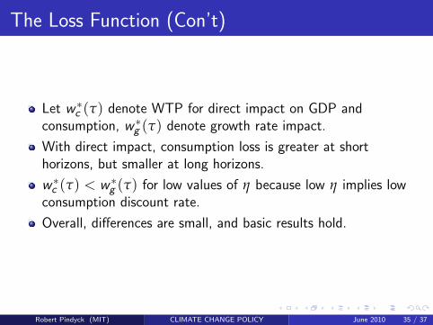

w ∗c (3) and w ∗
g (3), H = 100, g0 = .020, δ = 0
1 1.2 1.4 1.6 1.8 2 2.2 2.4 2.6 2.8 30
0.01
0.02
0.03
0.04
0.05
0.06
w*g(3) and w*
c(3), ∆T, β or γ Uncertain, H = 100, g
0 = .020, δ = 0
η
w* (3
)
w*g(3)
w*c(3)
Robert Pindyck (MIT) CLIMATE CHANGE POLICY June 2010 36 / 37
Conclusions and Caveats
Debate among economists is not whether to abate, but whethera stringent policy is needed now, or instead begin slowly.
My results support a “begin slowly” policy.
Dynamically efficient, accounts for technological change thatreduces abatement costs, and allows for learning.
Caveats are in order:
I used current consensus on the distributions for ∆T and itsimpact. Maybe consensus is wrong, especially about tails.We have very little data to assess, e.g., likelihood of ∆T > 5◦C,never mind its economic impact.I used linear loss function, but maybe convex relationshipbetween ∆T and the growth rate gt is more realistic.
Results also imply: Keep research focus on the tails.
Robert Pindyck (MIT) CLIMATE CHANGE POLICY June 2010 37 / 37

Conclusions and Caveats
Debate among economists is not whether to abate, but whethera stringent policy is needed now, or instead begin slowly.
My results support a “begin slowly” policy.
Dynamically efficient, accounts for technological change thatreduces abatement costs, and allows for learning.
Caveats are in order:
I used current consensus on the distributions for ∆T and itsimpact. Maybe consensus is wrong, especially about tails.
We have very little data to assess, e.g., likelihood of ∆T > 5◦C,never mind its economic impact.I used linear loss function, but maybe convex relationshipbetween ∆T and the growth rate gt is more realistic.
Results also imply: Keep research focus on the tails.
Robert Pindyck (MIT) CLIMATE CHANGE POLICY June 2010 37 / 37
Conclusions and Caveats
Debate among economists is not whether to abate, but whethera stringent policy is needed now, or instead begin slowly.
My results support a “begin slowly” policy.
Dynamically efficient, accounts for technological change thatreduces abatement costs, and allows for learning.
Caveats are in order:
I used current consensus on the distributions for ∆T and itsimpact. Maybe consensus is wrong, especially about tails.We have very little data to assess, e.g., likelihood of ∆T > 5◦C,never mind its economic impact.
I used linear loss function, but maybe convex relationshipbetween ∆T and the growth rate gt is more realistic.
Results also imply: Keep research focus on the tails.
Robert Pindyck (MIT) CLIMATE CHANGE POLICY June 2010 37 / 37

Conclusions and Caveats
Debate among economists is not whether to abate, but whethera stringent policy is needed now, or instead begin slowly.
My results support a “begin slowly” policy.
Dynamically efficient, accounts for technological change thatreduces abatement costs, and allows for learning.
Caveats are in order:
I used current consensus on the distributions for ∆T and itsimpact. Maybe consensus is wrong, especially about tails.We have very little data to assess, e.g., likelihood of ∆T > 5◦C,never mind its economic impact.I used linear loss function, but maybe convex relationshipbetween ∆T and the growth rate gt is more realistic.
Results also imply: Keep research focus on the tails.
Robert Pindyck (MIT) CLIMATE CHANGE POLICY June 2010 37 / 37

Conclusions and Caveats
Debate among economists is not whether to abate, but whethera stringent policy is needed now, or instead begin slowly.
My results support a “begin slowly” policy.
Dynamically efficient, accounts for technological change thatreduces abatement costs, and allows for learning.
Caveats are in order:
I used current consensus on the distributions for ∆T and itsimpact. Maybe consensus is wrong, especially about tails.We have very little data to assess, e.g., likelihood of ∆T > 5◦C,never mind its economic impact.I used linear loss function, but maybe convex relationshipbetween ∆T and the growth rate gt is more realistic.
Results also imply: Keep research focus on the tails.
Robert Pindyck (MIT) CLIMATE CHANGE POLICY June 2010 37 / 37