ANY OPINIONS EXPRESSED ARE THOSE OF THE AUTHOR(S) AND NOT NECESSARILY THOSE OF THE SCHOOL OF ECONOMICS & SOCIAL SCIENCES, SMU

SSSMMMUUU EEECCCOOONNNOOOMMMIIICCCSSS &&& SSSTTTAAATTTIIISSSTTTIIICCCSSS WWWOOORRRKKKIIINNNGGG PPPAAAPPPEEERRR SSSEEERRRIIIEEESSS

Un-balanced Economic Growth

Hing-Man Leung September 2007

Paper No. 12-2007

“Un-balanced” Economic Growth *

By Hing-Man Leung

Abstract: Since the elasticity of substitution between capital and labor is not always one, and

since technical progress is not always Harrod-neutral, it is desirable to have an endogenous

growth model that admits all sizes of the elasticity and all known technology modes. We derive

an equation to do just that, fully describing the per capita income growth rate at all times. It

shows a typical economy needing hundreds if not thousands of years to reach its long term

growth rate, leading to the conclusion that even the short run may be very long indeed.

JEL Classification: O10, O11, O12, 040

Keywords: The elasticity of substitution, Non-Harrod-neutral technology, short-run

growth

Address: School of Economics Singapore Management University 90 Stamford Road Singapore 178903

Telephone: +65 9852 7320 Fax: +65 6828 0833 E-mail: hmleung@smu.edu.sg

* I wish to thank Professor Olivier de La Grandville for discussion and encouragement, and the Singapore Management University Research Grant Number C244/MSS6E006 for financial support.

1. Introduction

Growth theory has traditionally focused on the so-called “balanced path.” This presupposes

either a unitary elasticity of substitution between capital and labor, or a Harrod-neutral mode of

technical change, or both. Despite efforts to justify these presuppositions, we are a long way

from being sure that they completely describe the world in which we live.1

If we are not sure about the size of the elasticity of substitution, then we should have a

model that admits all its plausible values, and work towards finding out how growth rates behave

under them. The same is true for the mode of technology. Thus is the aim of this paper: to build

an endogenous growth model that explicitly allows all conceivable elasticities, and all forms of

technical progress.

To do this, we derive a dynamic equation comprising four exogenous parameters on its

right-hand side, together with time t

ˆ( ) [ , , , (0), ]y t a b tσ φ= Ψ , (1)

where is the endogenous rate of per capita income growth, y σ is the elasticity of substitution

between capital and labor; a and b are defined in a general production function

, (2) ( ) [ ( ), ( )]at btY t F e K t e L t=

where Y is income or output, while (2) in turn implies the technology modes set out in (3) below

1 There is a growing recognition that the elasticity is typically not one, and often quite far from this number. For example, Arrow, Chenery, Minhas and Solow (1961, p. 226) showed that the United States of America in the first half of the twentieth century had “an over-all elasticity of substitution between capital and labor significantly less than unity”. Many studies since then, surveyed in Yuhn (1991, p. 343) reported U.S. elasticities not exceeding 0.76. Yuhn however found the Republic of Korea having a significantly higher σ , probably much closer to 1. Duffy and Papageorgiou (2000, p. 87) rejected the Cobb-Douglas, and found labor and capital “more substitutable in the richest group of countries and are less substitutable in the poorest group of countries”. Klump, McAdam and Wilmann (2004) found the elasticity of substitution well below unity for the U.S. economy from 1953 to 1998. Antràs (2004) concluded that the U.S. economy was not well described by a Cobb-Douglas aggregate production function. Zarembka (1970) and Bernt (1976) found elasticity close to but less than 1. In addition, papers such as Acemoglu’s “Directed Technical Change” (2002) remind us that technical change is not always Harrod-neutral.

1

(3) 0, 0 Harrod neutrality0, 0 Solow neutrality

0 Hicks neutrality ;

a ba ba b

= > ⇒⎧⎪ > = ⇒⎨⎪ = > ⇒⎩

the fourth variable, (0)φ , is the initial share of income earned by capital. We could have used

initial conditions instead of ˆ(0)y (0)φ , but that changes little. The important point is that all of

the exogenous variables in the system are on the right-hand side of (1); all those remaining and

not included in the equation, namely savings, capital formation, and the factor shares are

endogenously determined.

Using (1) we can plot the growth path precisely, and conduct comparative analysis in terms

of σ , a, b and (0)φ . Because of the familiarity with the balanced path, we contrarily call this the

un-balanced path. “Unbalanced” does not mean that growth behaves in some unwieldy way. By

contrast we find the economy neither collapses in the sense of failing to sustain itself, nor

dwindles to stagnation; instead it converges towards an asymptotic, constant, and positive growth

rate at least when the elasticity of substitution does not exceed one.

This dynamic equation has other uses, too. For instance, it helps us to find how long it takes

to converge to the long-term growth rate, and to answer: Just how long is the long run? It turns

out that the long run, and even the short run, is much longer than we previously thought. It takes

hundreds or sometimes thousands of years for the economy to gravitate to its long-term state.

Some economists asked “How long is the long run?” a few decades ago, for example

Atkinson (1969), Drandakis and Phelps (1966), and others. We give a very different answer here,

and our answer is more accurate because both K and ( )tφ are endogenous.

Our plan of the paper is as follows. Section two traces the factor shares, section three the

income growth path, both under Hicks-neutral technology with any elasticity. Section four

2

generalizes it to all technology types, comparing and contrasting between them, finding out

which technology mode is more growth-prone. Section five concludes the paper.

2. Tracing the Factor Shares

We want finally to be able to trace income growth, but to that end we first need to find the

path of the factor share. This share is interesting in its own right, depicting as it does the income

distribution as a nation grows.

We begin with a Hick-neutral technology. Write the homogeneous of degree one, strictly

concave-in-factors production function as

, (4) ( ) ( ) [ ( ), ( )]Y t A t F K t L t= ⋅

where Y, K, L and A are output, capital, labor and technology, respectively. Define capital’s share

as

( ) ( )( )( )

KY t K ttY t

φ ≡ , (5)

where and henceforth a subscript denotes a derivative. From (4) we have

( ) ( )( )( )

KF t K ttF t

φ ≡ . (6)

Let us denote any variable z’s time-derivative by ( ) ( )z t dz t dt≡ , its growth rate by

ˆ( ) ( ) ( )z t z t z t≡ , and keep the time reference implicit when possible. Differentiating (6) we get

ˆ ˆ ˆKF K Fφ ˆ= + − ;

differentiating we find [ ( ), ( )]F K t L t

ˆ ˆ ˆ ˆ( ) (1 )(K LF F K F Lφ φ= + + − + ˆ) ;

combining the last two equations we get

3

ˆ ˆ ˆ ˆ(1 )( ) KK L Fφ φ= − − + . (7)

All the variables in (7) are endogenous and can change over time, except L , but of that we have

no interests.

In its intensive form we can write ( , ) ( )F K L Lf k= , where k K L≡ , and K kF f= .

Differentiating it, and introducing the elasticity of substitution

( )k k

kk

f f k fk f f

σ −≡ − , (8)

we have

1ˆ ˆ(1 )( )KˆF K Lφ

σ= − − − . (9)

Substituting (9) into (7) we get

1ˆ ˆ ˆ(1 )(1 )( )K Lφ φσ

= − − − . (10)

A variant of equation (10) first appeared in Drandakis and Phelps (1966), and later in

Atkinson (1969). Notice in obtaining (10) we have not used any growth models, not even the

traditional assumption that a constant fraction of income is saved. We have merely assumed that

K and L are paid their competitive returns.

Using (10), we could be tempted to perform “back of an envelop” calculations to find ( )tφ .2

For instance, if σ is 0.7, K 20 per cent per year, L 2 per cent per year and φ 40 per cent, φ

would have fallen by about 4.6 per cent per year, and it would have taken merely 6.2 years for

the capital share to fall by ten percentage points. However, this is wrong, since K and φ on the

right-hand side of (10) are erroneously fixed. In fact we should be curious about (10): how could

2 See Atkinson (ibid.).

4

the rate of technical progress, A , not help determine capital’s share, even when the elasticity is

not unity? The correct answer is that indeed it should, as we will soon find out.

2.1 Integrating the differential equation

A straightforward first step is to eliminate ( )tφ from the right-hand side of (10), and then

replace it with its initial value. This turns out not to change much, but is nevertheless a necessary

step to take. Equation (10) can be written as

1 ˆ ˆ( ) ( )[1 ( )](1 )( )t t t Kφ φ φσ

= − − − L . (11)

Treating K and L as constant for now, we integrate (11) as a first-order differential

equation. Writing , this gives us ˆ ˆ ˆk K L≡ −

ˆ

ˆ ˆ(0)( )

[1 (0)] (0)

k t

k t k t

ete eσ

φφφ φ

=− +

, (12)

where (0)φ is the initial capital share.

( )tφ , according to (12), falls even faster than (10). We plot both paths using 0.7σ = ,

(0) 0.4φ = , and , and compare them in table 1 below. The ˆ 0.2K = ˆ 0.02L = ( )tφ row uses

equation (10), and the ( )*tφ row (12). Integrating for ( )tφ has not changed the numbers much,

suggesting erroneously a short run that is far shorter than it is.

Table 1

Year(t) 0 10 20 30 40 50 60 70 80 90 100 ( )tφ 0.400 0.252 0.159 0.101 0.063 0.040 0.025 0.016 0.010 0.006 0.004

( )tφ * 0.400 0.291 0.142 0.066 0.030 0.014 0.007 0.003 0.001 0.001 0.000 Key: the ( )tφ column uses equation (10); the ( )*tφ column uses equation (12).

5

2.2 Endogenizing K

Just as the share ( )tφ change over time, so does the rate of capital accumulation. While a

poor nation has meager means to accumulate capital, an emerging country saves and accumulates

vigorously to fuel growth, and a developed nation by contrast prefers spending to saving. Sub-

Saharan Africa, China, and the United States are obvious cases in point. I have examined the

World Development Indicators published by the World Bank, and found positive and statistically

significant time-trends for gross capital formation as a percentage of GDP for both the low- and

middle-income countries, but a negative trend for the developed ones. The need to endogenize

K is clear.

It is customary to model savings as a consequence of individual citizens maximizing their

discounted future utility from consumption. We normally take for granted the Ramsey utility

function

( ) 1( ) c tu tα

α−

= ,

where α , between 0 and 1, defines curvature and the speed at which marginal utility

diminishes as consumption increases. However, new evidence has emerged to question the

suitability of the Ramsey utility in studying growth. If we suddenly have twice as much to eat

and to wear, marginal utility would undoubtedly diminish. But if we have twice as much to eat

and wear in ten, twenty or even fifty year’s time, marginal utility would not fall quite as much, or

it may not fall at all since life-style, custom, and technology would have changed drastically by

then. It becomes even more problematic to assume diminishing marginal utility over hundreds or

more years. La Grandville (2006, 2007) has recently made a striking discovery that this Ramsey

utility yields an optimal savings rate approaching 100 percent of income within a few years for

any reasonable initial savings rates, leading him to question the appropriateness of the Ramsey

( ) 'u t s

6

formula. He further shows that replacing with , or in other words setting ( )u t ( )c t α to one,

produces a much more reasonable picture. We will follow Grandville, and work with

instead of .

( )c t

( )u t

L are workers as well as consumers, who consume in period t, giving rise to the

aggregate objective function

( )c t

, (13) 0

( ) ( )te c t L t dtρ∞ −∫

where ρ is a constant discount rate, and (13) is maximized subject to a savings-investment

constraint

[ ]( ) ( ) ( ), ( ) ( ) ( )K t A t F K t L t c t L t= ⋅ − . (14)

Dynamic optimization yields the Euler’s equation

( ) ( )KA t F t ρ= . (15)

Since ρ is constant, so is . Differentiating this and suppressing the time reference

we have

( ) ( )KA t F t

K KF F A A μ= − = − . This constancy of KAF governs optimal savings. If 0μ = ,

people save and invest in order to keep KF constant, and that means keeping K K abreast with

the exogenous L L . However if 0μ > , we have an additional incentive to save and to add to the

capital stock. Each unit of new capital alters the marginal product KF in a way dictated by the

elasticity of substation between capital and labor, for that reason the elasticity plays a crucial role

in the process of endogenous growth.

In intensive form we have ( ) whereY Ky A f k kL L

≡ = ⋅ ≡ , and thus ( , ) ( )K kF K L f k= .

Differentiating it we get K kkF f= k , where kkf is the second-derivative with respect to k , and we

can write

7

[ ]K K kk kF F f f k= . (16)

Using (16), the elasticity of substitution ( )k

kk

kf f k fk f f

σ −≡ − , and K KF F μ= − we have

k L

k fk f k f LF

μσ μσ⎡ ⎤ F⎡ ⎤

= =⎢ ⎥ ⎢ ⎥− ⎣ ⎦⎣ ⎦. (17)

Since LF LF is the inverse of the share of labor in national income, we can write

(1 )kk

μσ= −φ . Substituting this into (12) we have

( ) ( ) ( 1)t tφ φ μ σ= − ,

and from which we obtain an equation defining the time-path of capital’s share

( ) (0) exp[ ( 1) ]t tφ φ μ σ= − . (18)

Assume 0.02μ = , 0.7σ = , and (0) 0.4φ = as before, we plotted ( )tφ ** using (18), in table

2. The numbers from table 1 are included for comparison.

Table 2: The endogenous share of capital ( )tφ

Year(t) 0 10 20 30 40 50 60 70 80 90 100 ( )tφ 0.400 0.252 0.159 0.101 0.063 0.040 0.025 0.016 0.010 0.006 0.004 ( )tφ * 0.400 0.291 0.142 0.066 0.030 0.014 0.007 0.003 0.001 0.001 0.000 ( )tφ ** 0.400 0.377 0.355 0.334 0.315 0.296 0.279 0.263 0.248 0.233 0.220

Key: ( )tφ and ( )tφ * are values taken from table 1.

The difference between the bottom row and the other rows speaks volumes about the

importance of endogenizing . The technology progress rate ( )K t μ plays a pivotal role in (18);

for instance a larger μ speeds up the decline of capital’s share, when capital is not good enough

a substitute for labor (σ is less than 1). This is precisely what we would expect, because then

8

capital’s marginal reward falls disproportionately faster than capital is added to production. In

addition, capital accumulates more rapidly the larger is μ .

The long run seems quite long, taking hundreds of years for the factor shares to change

significantly. The factor share path gives a glimpse of what a country’s growth path might look

like – per capita income probably takes just as long to change as the factor share. This conjecture

will be proved correct in what follows. However, it is imperative to know precisely how

behaves over time because, as it turns out, the shares path misses something critical, making it a

poor proxy for gauging the incomes path. We will soon verify this.

y

3. The Incomes Path

We will find in the next section a dynamic income growth equation that admits all three

technology modes, but for the moment focus only on the Hicks-neutral technology.

Differentiating KF K Fφ = we may write

ˆˆ ˆ ˆKF F K φ= + − . (19)

Since technology is Hicks-neutral, we can use ˆ ( 1φ μ σ )= − from (18) in (19) to get

ˆ ˆF K μσ= − . (20)

From (17) we also have

ˆ ˆ(1 )

K Lμσφ

= +−

. (21)

Using (21) in (20), adding μ to both sides and noting ˆ ˆy Fμ L= + − , we have

( )ˆ( ) 11 ( )

ty tt

φμ σφ

⎡ ⎤⎛ ⎞= +⎢ ⎥⎜ ⎟−⎝ ⎠⎣ ⎦

. (22)

9

Substituting to eliminate ( )tφ using (18), we have an income growth path entirely in terms

of the exogenous parameters and t

exp[ ]ˆ( ) 1 (0)exp[ ] exp[ ] (0)

ty tt t

μσμ φ σμ μσ φ

⎧ ⎫⎛ ⎞⎪ ⎪= +⎨ ⎬⎜ −⎪ ⎪⎝ ⎠⎩ ⎭⎟ . (23)

We may sometimes want to consider

ˆ( ) exp[ ]1 (0)

exp[ ] exp[ ] (0)y t t

t tμσφ σ

μ μ μσ⎛

= + ⎜ −⎝ ⎠φ⎞⎟ , (24)

which is the per capita income growth for each percentage technical improvement μ . There are

three cases to consider.

3.1 1σ =

Substituting 1σ = into (24) we get

ˆ( ) 1

1 (0y t

)μ φ=

−. (25)

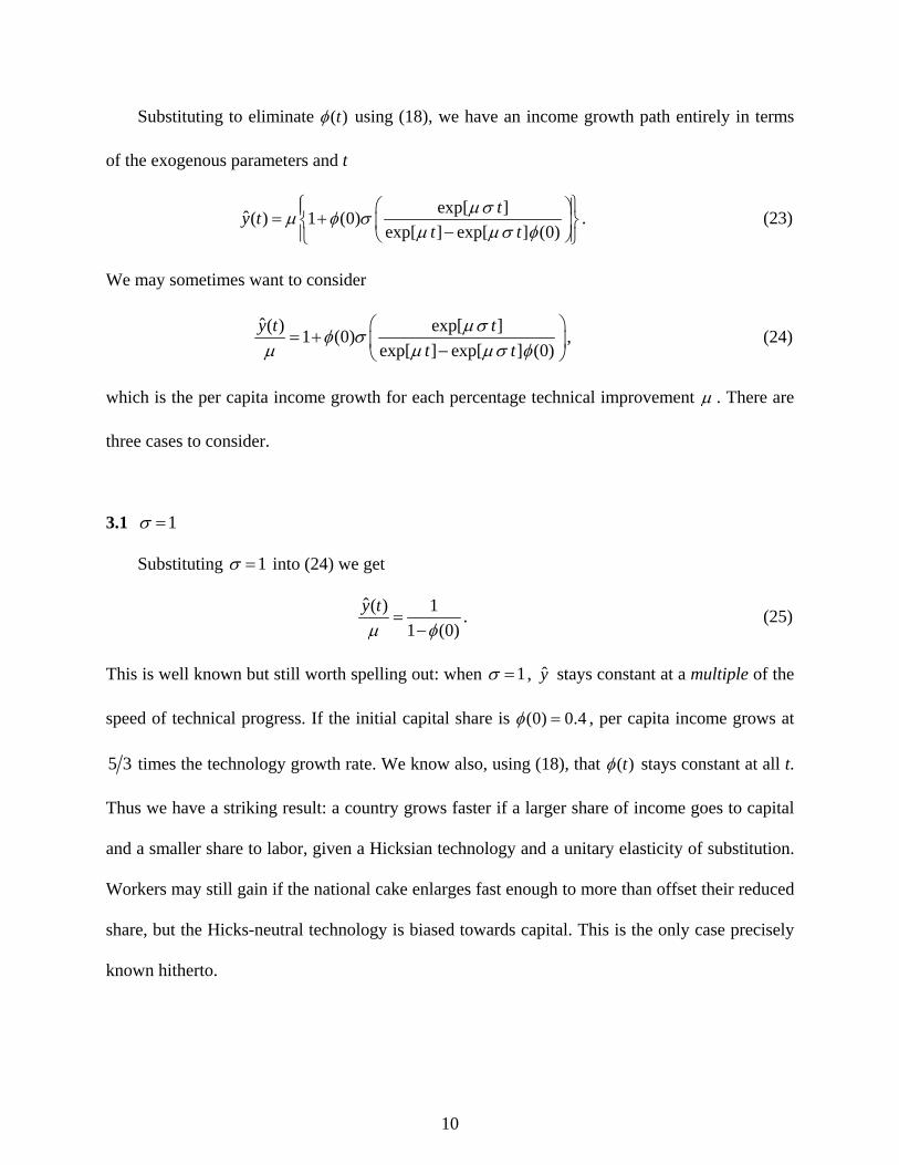
This is well known but still worth spelling out: when 1σ = , stays constant at a multiple of the

speed of technical progress. If the initial capital share is

y

(0) 0.4φ = , per capita income grows at

5 3 times the technology growth rate. We know also, using (18), that ( )tφ stays constant at all t.

Thus we have a striking result: a country grows faster if a larger share of income goes to capital

and a smaller share to labor, given a Hicksian technology and a unitary elasticity of substitution.

Workers may still gain if the national cake enlarges fast enough to more than offset their reduced

share, but the Hicks-neutral technology is biased towards capital. This is the only case precisely

known hitherto.

10

3.2 1σ <

Differentiating the fractional term in (24) with respect to t we get

{ }2

exp[ (1 )] (1 )exp[ ]exp[ ] exp[ ] (0) exp[ ] exp[ ] (0)

ttd dtt t t t

μ σ μ σμσμ μσ φ μ μσ φ

⎛ ⎞ + −= −⎜ ⎟− −⎝ ⎠

, (26)

which is negative for 1σ < . From this we know must be falling at all t. ˆ ( )y t

It is easy to verify that for all 1σ < ,

( )

exp[ ] 0exp[ ] exp[ ] (0)

t

tLimt t

μσμ μσ φ

→∞

⎛ ⎞=⎜ ⎟−⎝ ⎠

. (27)

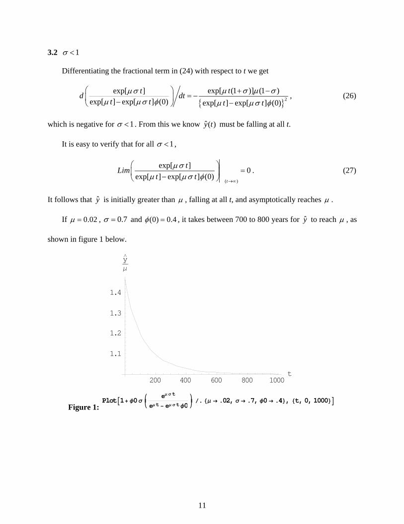
It follows that is initially greater than y μ , falling at all t, and asymptotically reaches μ .

If 0.02μ = , 0.7σ = and (0) 0.4φ = , it takes between 700 to 800 years for to reach y μ , as

shown in figure 1 below.

200 400 600 800 1000t

1.1

1.2

1.3

1.4

yfl

μ

Figure 1: PlotA1+ φ0σ

ik

μ σ t

μ t− μ σ t φ0y{ê.8μ → .02, σ → .7, φ0 → .4<, 8t, 0, 1000<E

11

Increasing σ towards 1 lengthens the time needed to reach μ , which makes sense because

of what we found in section 3.1 above. Figure 2 below shows that if σ goes from 0.7 to 0.8,

takes thousands instead of hundreds of years to reach

y

μ .

2000 4000 6000 8000 10000t

1.01

1.02

1.03

1.04

1.05

1.06

yfl

μ

Figure 2: PlotA1+ φ0σ

ik

μ σ t

μ t − μ σ t φ0y{ê.8μ → .02, σ → .9, φ0 → .4<, 8t, 0, 10000<E

Using (24) we can plot any growth path using whatever parameter values we deem suitable.

Generally speaking, a larger μ , a smaller σ , and a larger (0)φ make the curve steeper, shifting

it to the left, shortening the short-run; and conversely. For as long as 1σ < , gravitates towards y

μ , and it takes longer to do so if σ is closer to 1. If σ reaches 1, however, jumps abruptly

and permanently to

y

1 [1 ( )]tφ− times μ , whereupon ( )tφ itself becomes a constant. In this way,

σ controls a “gearing” mechanism, leveraging upwards, using y μ as a base.

12

3.3 1σ >

It is common knowledge that 1σ > leads to an upwardly explosive growth, and ˆ 0dy dt >

from (26) reinforces that belief. It is interesting, nonetheless, to plot a typical path using (24), as

we have done in figure 3.

200 400 600 800 1000

-60

-40

-20

20

40

60

Figure 3: PlotA1 + φ0 σ

ik

μ σ t

μ t − μ σ t φ0y{ê. 8μ → .02, σ → 1.2, φ0 → .4<, 8t, 0, 1000<E

It first appears that the path turns from +∞ to −∞ at some t above 200 years; but from (18),

( )tφ becomes unity at exactly 229.073 years using the parameters in figure 3, and from that point

on capital receives more than 100 per cent of national income. We must therefore rule out the

region to the right of 229.073 years in figure 3.

Growth positively explodes at some finite time for all 1σ > . A larger μ , a larger σ , or a

larger (0)φ bring that explosive date sooner. Although we know very little what explosive

growth means in practice, a larger σ without doubt is growth-promoting.

13

4. A General Technology

Instead of the Hicks-neutral (4) suppose we have

. (28) ( ) [ ( ), ( )], ( ) ( ) ( ), , 0at btY t F G t H t G e K t and H t e L t a b= ≡ ≡ >

The variables G and H stand for efficiency units of capital and labor. If we are back to a b=

(4) and the conclusions reached there apply. The capital ˆ ( )K t comes from endogenous savings

as before, and ˆ( )L t is assumed exogenously constant. Our aim here is to discover which

technology mode yields faster income growth. Recall from (3) that a describes a more

Solow-neutral mode, etc. We first need an equation for the factor shares.

b

4.1 The factor shares

We will show that the factor shares path is completely independent of b , but the incomes

path is not. Consequently, the factor share is a poor proxy for the income growth path.

Differentiating (28), rearranging it, and analogous to (10) we get

1ˆ ˆ ˆ(1 )(1 )[( ) ( )]a b K Lφ φσ

= − − − + − . (29)

The variables φ , K and L on the right-hand side are endogenous, but we can find them using

the method used before.

Notice that the aggregate consumption term in the investment equation is in terms of L and

not H . Physical capital accumulates according to

, (30) ( ) [ ( ), ( )] ( ) ( )K t F G t H t c t L t= −

and the Hamiltonian, denoted Γ since H is efficiency labor, is

( ) ( ) ( ) { [ ( ), ( )] ( ) ( )}t c t L t F G t H t c t L tθΓ = − − . (31)

Keeping the time-reference implicit, the Euler equation is

14

atGe F ρ= . (32)

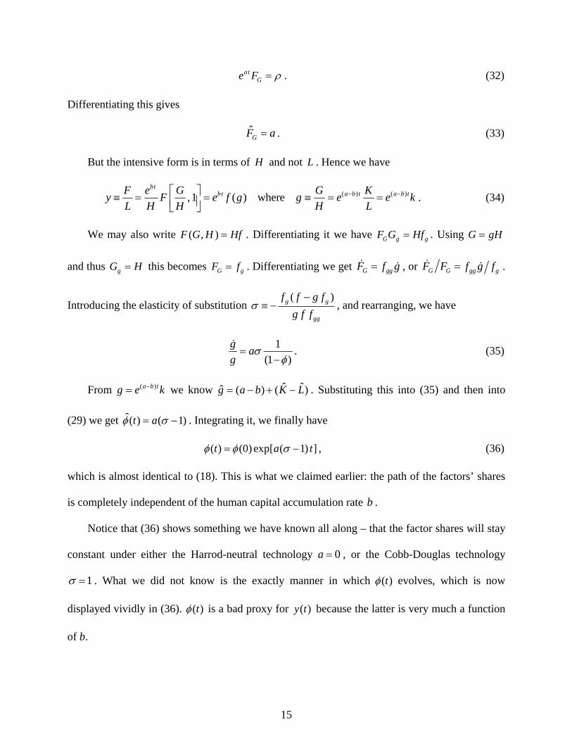
Differentiating this gives

GF a= . (33)

But the intensive form is in terms of H and not L . Hence we have

( ) ( ),1 ( ) wherebt

bt a b t a b tF e G G Ky F e f g g e eL H H H L

− −⎡ ⎤≡ = = ≡ = =⎢ ⎥⎣ ⎦k . (34)

We may also write . Differentiating it we have ( , )F G H Hf= G g gF G Hf= . Using G gH=

and thus this becomes . Differentiating we get , or gG H= GF f= g gG ggF f= G G gg gF F f g f= .

Introducing the elasticity of substitution ( )g g

gg

f f g fg f f

σ−

≡ − , and rearranging, we have

1(1 )

g ag

σφ

=−

. (35)

From we know . Substituting this into ( )a b tg e k−= ˆ ˆˆ ( ) (g a b K L= − + − )

t

(35) and then into

(29) we get . Integrating it, we finally have ˆ( ) ( 1)t aφ σ= −

( ) (0) exp[ ( 1) ]t aφ φ σ= − , (36)

which is almost identical to (18). This is what we claimed earlier: the path of the factors’ shares

is completely independent of the human capital accumulation rate . b

Notice that (36) shows something we have known all along – that the factor shares will stay

constant under either the Harrod-neutral technology 0a = , or the Cobb-Douglas technology

1σ = . What we did not know is the exactly manner in which ( )tφ evolves, which is now

displayed vividly in (36). ( )tφ is a bad proxy for because the latter is very much a function

of b.

( )y t

15

4.2 The income path

Differentiating ( )bty e f g= from (34) we have

ˆy b f= + . (37)

Notice gf f g= , and thus

ˆgg ff g gf f g

φ= = . (38)

Using this and (35) in (37) we have

( )ˆ( )[1 ( )]

ty t b at

φσφ

= +−

. (39)

Using (36), we finally have

(0)exp[ ( 1) ]ˆ( )1 (0)exp[ ( 1) ]

a ty t b aa t

φ σσφ σ

−= +

− −. (40)

It is straightforward to check that is constant if either ˆ( )y t 1σ = , or 0a = and . 0b >

Two results emerge immediately. First, there is a one-to-one positive relationship between

the human capital and the per capita incomes growth rate b, even though b has no impact on

( )tφ .

Second, the relations between and a is a complex one. If ˆ( )y t 1σ < , the exponential terms

go to 0 as t goes to infinity, and asymptotically converges to b. Since that takes a very long

time to happen, it is important to know more than just the asymptote. To get a clearer picture we

can differentiate

ˆ( )y t

(40) with respect to a to get

{ }{ }2

(0)exp[ ( 1) ] 1 (1 ) (0)exp[ ( 1) ]ˆ( )1 (0)exp[ ( 1) ]

a t at a tdy tda a t

φ σ σ φ σ

φ σ

− − − − −=

− −, (41)

which when plotted yields figure 4.

16

100 200 300 400 500t

-0.04

-0.02

0.02

0.04

0.06

d yfl

da

Figure 4:

PlotA−atH−1+σLσ φ0H−1+ aHt− tσL+ atH−1+σLφ0L

H−1+ atH−1+σL φ0L2ê.8φ0 → .4, σ → .7, a → .05<, 8t, 0, 500<E

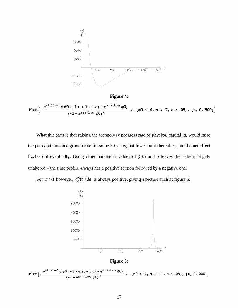
What this says is that raising the technology progress rate of physical capital, a, would raise

the per capita income growth rate for some 50 years, but lowering it thereafter, and the net effect

fizzles out eventually. Using other parameter values of (0)φ and a leaves the pattern largely

unaltered – the time profile always has a positive section followed by a negative one.

For 1σ > however, ˆ( )dy t da is always positive, giving a picture such as figure 5.

50 100 150 200t

5000

10000

15000

20000

25000

d yfl

da

17

Figure 5:

PlotA−atH−1+σL σ φ0H−1 + aHt− t σL + atH−1+σL φ0L

H−1+ atH−1+σL φ0L2ê.8φ0 → .4, σ → 1.1, a → .05<, 8t, 0, 200<E

Using our previous reasoning, ˆ( )dy t da after the spike at about 185 years is not meaningful

since ( )tφ would then have reached 1.

As an exercise suppose . Figure 6 gives a slide-show of reducing a and

increasing b, keeping their sum equal to 0.06. As the technology mode shifts towards Harrod-

neutral from Solow-neutral (increasing b and decreasing a), the curve in figure 6 shifts towards

the northeast direction. Improving human capital leads to a faster and longer lasting growth, than

improving the efficiency of physical capital.

0.06a b+ =

100 200 300 400 500t

0.0025

0.005

0.0075

0.01

0.0125

0.015

yfl

100 200 300 400 500t

0.0225

0.025

0.0275

0.03

0.0325

0.035

0.0375

yfl

0.06, 0a b= = 0.04, 0.02a b= =

200 400 600 800 1000t

0.042

0.044

0.046

0.048

yfl

200 400 600 800 1000t

0.02

0.04

0.06

0.08

0.1

0.12

yfl

0.02, 0.04a b= = 0, 0.06a b= =

Figure 6: plotting using equation ˆ( )y t (40), and 0.7σ = , (0) 0.4φ =

18

5. Conclusions

Some findings in the foregoing are familiar, the others are relatively new. The major ones

may be summarized more systematically as follows.

1. A larger elasticity of substitution in general leads to faster and longer-lasting growth in

per capita income.

2. A more Harrod-neutral type of technical progress has more growth-promoting properties,

than a more Solow-neutral type.

3. It is quite sensible to talk about long-term growth when the elasticity of substitution

between capital and labor is not one. Even the short-run is quite long, taking hundreds or

more years for the growth rate to settle to its long-term constant rate. It is time we

focused more on phenomena other than the “balanced path.”

4. Similarly it is quite reasonable to talk about the non-Harrod-neutral growth. A rise in the

technical progress rate has very long-lasting benefits on income growth.

The main theoretical contribution of this paper is the derivation of a dynamic growth

equation that is much more general than what we have known from the literature. This equation

allows all elasticities and all technology modes, as shown in (40). It should be straightforward to

test this equation empirically, if we have good data, and good estimates of the elasticities and the

other variables. The incomes and the factor shares paths have something in common – they both

take hundreds of years to return to their long term level. Even when there are limited

opportunities to substitute capital for labor—when the elasticity of substitution is low—and even

when physical capital improves faster than human capital, each mode of technical change have

prolonged boosting effects on income which, over time, accumulates to tremendous

improvements on our standards of living.

19

References

Acemoglu, Daron. “Directed Technical Change”. Review of Economic Studies, October 2002, 69(4), pp. 749-1017.

Antràs, Pol. “Is the U.S. Aggregate Production Function Cobb-Douglas? New Estimates of the

Elasticity of Substitution”. Contributions to Macroeconomics, 2004, 4(1), pp. 1-34. Arrow, Kenneth J.; Chenery, Hollis B.; Minhas, Bagicha S. and Solow, Robert M. “Capital-

Labour Substitution and Economic Efficiency”. Review of Economics and Statistics, August 1961, 43(3), pp. 225-247.

Atkinson, Antony B. “The Timescale of Economic Models: How Long is the Long Run”?

Review of Economic Studies, April 1969, 36(2), pp. 137-152. Bernt, Ernst R. “Reconciling Alternative Estimates of the Elasticity of Substitution”. Review of

Economics and Statistics, February 1976, 58(1), pp. 59-68. De La Grandville, Olivier. “Optimal Growth, the Optimal Savings Rate and the Elasticity of

Substitution”. Paper presented at the CES Conference, Eltville, Germany, 2006. De La Grandville, Olivier. Economic Growth – A Unified Approach. Manuscript, 2007. Drandakis, E. M; Phelps, Edmund S. “A Model of Induced Inventions, Growth and

Distribution”. Economic Journal, December 1966, 76(304), pp. 823-840. Duffy, John and Papageorgiou, Chris. “A Cross-Country Empirical Investigation of the

Aggregate Production Function Specification”. Journal of Economic Growth, March 2000, 5(1), pp. 87-120.

Klump, Rainer; McAdam, Peter and Willman, Alpo. “Substitution and Factor Augmenting

Technical Progress in the US: A Normalized Supply-Side System Approach”. European Central Bank Working Paper Series, June 2004, No. 367.

Yuhn, Ky-hyang. “Economic Growth, Technical Change Biases, and the Elasticity of

Substitution: A Test of the De La Grandville Hypothesis”. Review of Economics and Statistics, May 1991, 73(2), pp. 340-346.

Zarembka, Paul. “On the Empirical Relevance of the CES Production Function”. Review of

Economics and Statistics, February 1970, 52(1), pp. 47-53.

20