un approccio ``libero'' alla moderna aeroelasticità ... coupling of structural and...
TRANSCRIPT

POLITECNICO DI MILANO
Corso di Laurea in Ingegneria Aeronautica
Un approccio “libero” alla modernaAeroelasticita Computazionale
Relatore: Prof. Paolo Mantegazza
Tesi di Laurea di:
Giulio Romanelli matr. 679778
Elisa Serioli matr. 679777
Anno Accademico 2007/2008
Un approccio “libero” alla moderna Aeroelasticita Computazionale
Introduction Structural system Aerodynamic system Coupling procedure Aeroelastic system Conclusions
Introduction
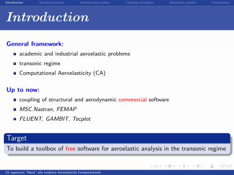
General framework:
academic and industrial aeroelastic problems
transonic regime
Computational Aeroelasticity (CA)
Up to now:
coupling of structural and aerodynamic commercial software
MSC.Nastran, FEMAP
FLUENT, GAMBIT, Tecplot
Target
To build a toolbox of free software for aeroelastic analysis in the transonic regime
Un approccio “libero” alla moderna Aeroelasticita Computazionale

Introduction Structural system Aerodynamic system Coupling procedure Aeroelastic system Conclusions
Block diagram
Post-processorPre/Post-processor Mesh generator
ParaViewGmshSalome
Aeroelastic Solver
Aerodynamic SolverStructural Solver
Aeroelastic Interface
OpenFOAMCode Aster
NAEMO MASSA
Linear interpolation
Build [Ham(k, M∞) ] Build V∞ − ω, V∞ − g
Un approccio “libero” alla moderna Aeroelasticita Computazionale

Introduction Structural system Aerodynamic system Coupling procedure Aeroelastic system Conclusions
Free software
Definition:
Fundamental freedoms by R. Stallmanand Free Software Foundation (1986):
1 run the program for any purpose
2 study and modify the program
3 copy the program
4 improve the program and releasethe improvements to the public,so the whole community benefits
source code available
freedom not price
copyleft licences GNU GPL and LGPL
Un approccio “libero” alla moderna Aeroelasticita Computazionale
Introduction Structural system Aerodynamic system Coupling procedure Aeroelastic system Conclusions
Structural solver
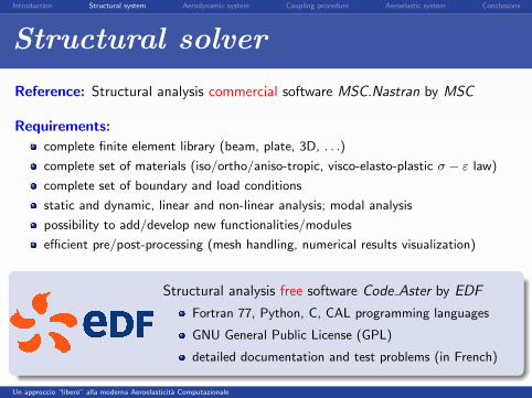
Reference: Structural analysis commercial software MSC.Nastran by MSC
Requirements:
complete finite element library (beam, plate, 3D, . . .)
complete set of materials (iso/ortho/aniso-tropic, visco-elasto-plastic σ − ε law)
complete set of boundary and load conditions
static and dynamic, linear and non-linear analysis; modal analysis
possibility to add/develop new functionalities/modules
efficient pre/post-processing (mesh handling, numerical results visualization)
Structural analysis free software Code Aster by EDF
Fortran 77, Python, C, CAL programming languages
GNU General Public License (GPL)
detailed documentation and test problems (in French)
Un approccio “libero” alla moderna Aeroelasticita Computazionale
Introduction Structural system Aerodynamic system Coupling procedure Aeroelastic system Conclusions
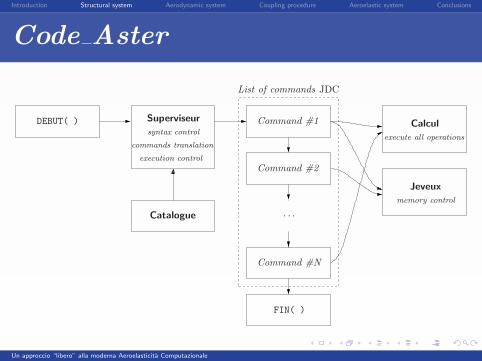
Code Aster
· · ·
DEBUT( )
FIN( )
List of commands JDC
Catalogue
Superviseur
Jeveux
CalculCommand #1
Command #2
Command #N
syntax control
commands translation
execution control
execute all operations
memory control
Un approccio “libero” alla moderna Aeroelasticita Computazionale
Introduction Structural system Aerodynamic system Coupling procedure Aeroelastic system Conclusions
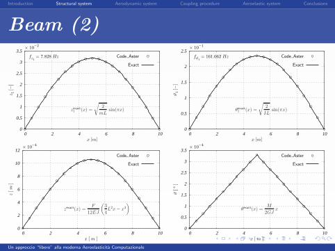
Beam (1)
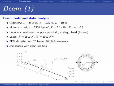
Beam modal and static analysis:
Geometry: R = 0.15 m, e = 0.05 m, L = 10 m
Material: steel, ρ = 7800 kg/m3, E = 2.1 · 1011 Pa, ν = 0.3
Boundary conditions: simply supported (bending), fixed (torsion)
Loads: F = 2500 N , M = 5000 Nm
FEM dicretization: 20 beam (POU D E) elements
comparison with exact solution
e
Rx
y
y
z z
L
m, I, EJ, GJ
MF
=
=
sx = 0
sy = 0
sz = 0
θx = 0
sx = 0
sy = 0
sz = 0
θx = 0
Un approccio “libero” alla moderna Aeroelasticita Computazionale
Introduction Structural system Aerodynamic system Coupling procedure Aeroelastic system Conclusions
Beam (2)
0
0.5
1
1.5
2
2.5
3
3.5
0 2 4 6 8 10
z1 [−
]
x [m]
¯fz1
= 7.828 Hz
× 10−2
Code Aster
Exact
zexact1 (x) =
√
2
mLsin(πx)
0
0.5
1
1.5
2
2.5
0 2 4 6 8 10
ϑ1 [−
]
x [m]
¯fϑ1
= 161.062 Hz
× 10−1
Code Aster
Exact
θexact1 (x) =
√
2
ILsin(πx)
0
2
4
6
8
10
12
0 2 4 6 8 10
z [
m]
x [ m ]
¯
× 10−4
Code Aster
Exact
zexact(x) =
F
12EJ
(
3
4L
2x− x
3
)
0
0.5
1
1.5
2
2.5
3
3.5
0 2 4 6 8 10
ϑ [
°]
x [ m ]
¯
× 10−4
Code Aster
Exact
θexact(x) =M
2GJx
Un approccio “libero” alla moderna Aeroelasticita Computazionale
Introduction Structural system Aerodynamic system Coupling procedure Aeroelastic system Conclusions
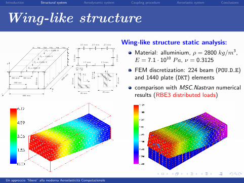
Wing-like structure
x
y
z
bxbx
by
by=
=
=
=
F1 = 13200 N
F2 = 13200 N
F3 = 13200 N
F4 = 6600 N
1600mm
600 mm
200 mm200 mm
300
mm
300 mm 25
mm
25
mm
25 mm20 mm
3.2
mm
2.5 mm2.5 mm2.5 mm
2.5 mm
1.5 mm 1.5 mm
2.0
mm
3.0
mm
Wing-like structure static analysis:
Material: alluminium, ρ = 2800 kg/m3,E = 7.1 · 1010 Pa, ν = 0.3125
FEM discretization: 224 beam (POU D E)and 1440 plate (DKT) elements
comparison with MSC.Nastran numericalresults (RBE3 distributed loads)
Un approccio “libero” alla moderna Aeroelasticita Computazionale
Introduction Structural system Aerodynamic system Coupling procedure Aeroelastic system Conclusions
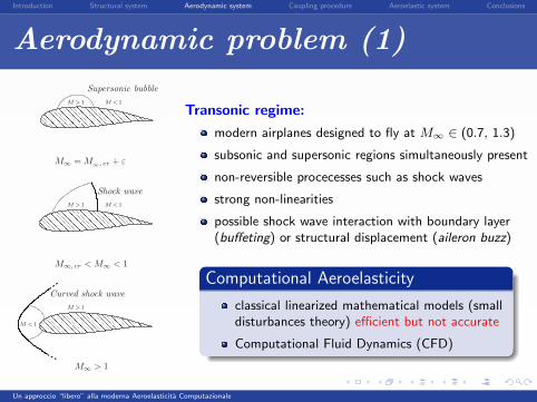
Aerodynamic problem (1)
Supersonic bubble
Shock wave
Curved shock wave
M∞ = M∞, cr + ε
M∞, cr < M∞ < 1
M∞ > 1
M >1
M >1
M >1
M <1
M <1
M <1
Transonic regime:
modern airplanes designed to fly at M∞ ∈ (0.7, 1.3)
subsonic and supersonic regions simultaneously present
non-reversible procecesses such as shock waves
strong non-linearities
possible shock wave interaction with boundary layer(buffeting) or structural displacement (aileron buzz)
Computational Aeroelasticity
classical linearized mathematical models (smalldisturbances theory) efficient but not accurate
Computational Fluid Dynamics (CFD)
Un approccio “libero” alla moderna Aeroelasticita Computazionale
Introduction Structural system Aerodynamic system Coupling procedure Aeroelastic system Conclusions
Aerodynamic problem (2)
Mathematical models: compromise between accuracy and efficiency
1 Full potential equations (1 unknown per cell)
omoentropic irrotational flow but OK up to M∞ = 1.3÷ 1.4
linearized wake models for lifting bodies
2 Euler equations (Nd + 2 unknowns per cell)
high Re, thin boundary layer, moderate α
accurate prediction of pressure distribution
3 Reynolds Averaged Navier Stokes equations (Nd + 2 + Nt unknowns per cell)
accurate prediction of aerodynamic lift and drag loads
no free software to create boundary layer meshes
Un approccio “libero” alla moderna Aeroelasticita Computazionale
Introduction Structural system Aerodynamic system Coupling procedure Aeroelastic system Conclusions
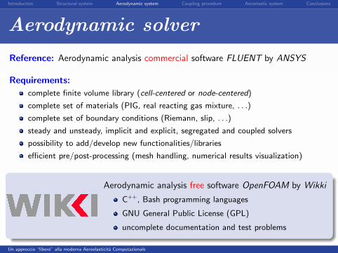
Aerodynamic solver
Reference: Aerodynamic analysis commercial software FLUENT by ANSYS
Requirements:
complete finite volume library (cell-centered or node-centered)
complete set of materials (PIG, real reacting gas mixture, . . .)
complete set of boundary conditions (Riemann, slip, . . .)
steady and unsteady, implicit and explicit, segregated and coupled solvers
possibility to add/develop new functionalities/libraries
efficient pre/post-processing (mesh handling, numerical results visualization)
Aerodynamic analysis free software OpenFOAM by Wikki
C++, Bash programming languages
GNU General Public License (GPL)
uncomplete documentation and test problems
Un approccio “libero” alla moderna Aeroelasticita Computazionale
Introduction Structural system Aerodynamic system Coupling procedure Aeroelastic system Conclusions
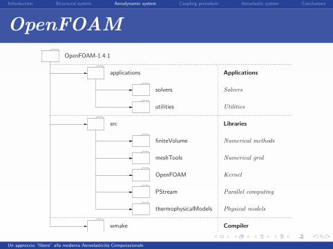
OpenFOAM
OpenFOAM-1.4.1
applications
solvers
utilities
Applications
Solvers
Utilities
src
finiteVolume
meshTools
OpenFOAM
PStream
thermophysicalModels
wmake
Libraries
Numerical methods
Numerical grid
Kernel
Parallel computing
Physical models
Compiler
Un approccio “libero” alla moderna Aeroelasticita Computazionale

Introduction Structural system Aerodynamic system Coupling procedure Aeroelastic system Conclusions
Evaluation of existing solvers (1)
L = 4.17 m
h=
1m
α1 α2 =
θθ
v1v2
v2
v3
1©
2©
3©M1, P1, T1
M2, P2, T2
M3, P3, T3
2D Oblique shock reflection
M∞ = 2.9, α1 = 29
comparison with exact solution
PC AMD64 2.2 Ghz, 1 Gbyte RAM
(A) Ne = 40 × 10 = 400 ∆t = 4·10−5 (B) N
e = 80 × 20 = 1600 ∆t = 2·10−5
(C) Ne = 160 × 40 = 6400 ∆t = 1·10−5 (D) N
e = 320 × 80 = 25600 ∆t = 5·10−6
Un approccio “libero” alla moderna Aeroelasticita Computazionale
Introduction Structural system Aerodynamic system Coupling procedure Aeroelastic system Conclusions
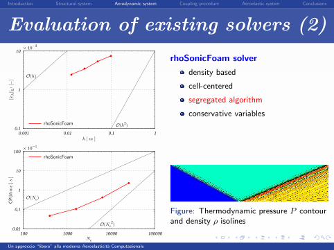
Evaluation of existing solvers (2)
0.1
1
10
0.001 0.01 0.1 1
||eh||
L1 [−
]
h [ m ]
O(h)
O(h2)
× 10−2
rhoSonicFoam
rhoSonicFoam solver
density based
cell-centered
segregated algorithm
conservative variables
0.01
0.1
1
10
100
100 1000 10000 100000
CPU
tim
e [
s]
Ne
O(Ne)
O(Ne
2)
× 10−1
rhoSonicFoam
Figure: Thermodynamic pressure P contourand density ρ isolines
Un approccio “libero” alla moderna Aeroelasticita Computazionale
Introduction Structural system Aerodynamic system Coupling procedure Aeroelastic system Conclusions
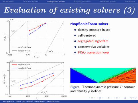
Evaluation of existing solvers (3)
0.1
1
10
0.001 0.01 0.1 1
||eh||
L1 [−
]
h [ m ]
O(h)
O(h2)
× 10−2
rhopSonicFoam
rhoSonicFoam
rhopSonicFoam solver
density-pressure based
cell-centered
segregated algorithm
conservative variables
PISO correction loop
0.01
0.1
1
10
100
100 1000 10000 100000
CPU
tim
e [
s]
Ne
O(Ne)
O(Ne
2)
× 10−1
rhoSonicFoam
rhopSonicFoam
Figure: Thermodynamic pressure P contourand density ρ isolines
Un approccio “libero” alla moderna Aeroelasticita Computazionale
Introduction Structural system Aerodynamic system Coupling procedure Aeroelastic system Conclusions
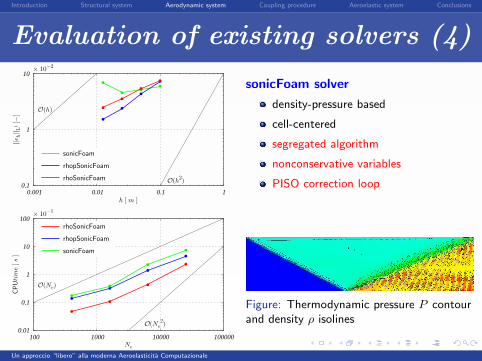
Evaluation of existing solvers (4)
0.1
1
10
0.001 0.01 0.1 1
||eh||
L1 [−
]
h [ m ]
O(h)
O(h2)
× 10−2
sonicFoam
rhopSonicFoam
rhoSonicFoam
sonicFoam solver
density-pressure based
cell-centered
segregated algorithm
nonconservative variables
PISO correction loop
0.01
0.1
1
10
100
100 1000 10000 100000
CPU
tim
e [
s]
Ne
O(Ne)
O(Ne
2)
× 10−1
rhoSonicFoam
rhopSonicFoam
sonicFoam
Figure: Thermodynamic pressure P contourand density ρ isolines
Un approccio “libero” alla moderna Aeroelasticita Computazionale
Introduction Structural system Aerodynamic system Coupling procedure Aeroelastic system Conclusions
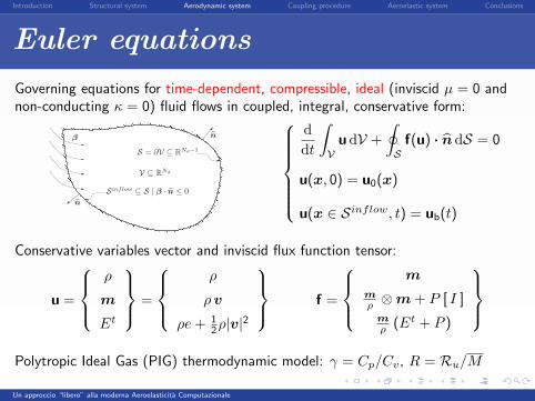
Euler equations
Governing equations for time-dependent, compressible, ideal (inviscid µ = 0 andnon-conducting κ = 0) fluid flows in coupled, integral, conservative form:
V ⊆ RNd
S = ∂V ⊆ RNd−1
β
Sinflow ⊆ S | β · n ≤ 0
n
n
ddt
∫V
udV +
∮S
f(u) · n dS = 0
u(x, 0) = u0(x)
u(x ∈ Sinflow, t) = ub(t)
Conservative variables vector and inviscid flux function tensor:
u =
ρ
m
Et
=
ρ
ρ v
ρe + 12ρ|v|2
f =
m
mρ ⊗m + P [ I ]
mρ (Et + P )
Polytropic Ideal Gas (PIG) thermodynamic model: γ = Cp/Cv, R = Ru/M
Un approccio “libero” alla moderna Aeroelasticita Computazionale

Introduction Structural system Aerodynamic system Coupling procedure Aeroelastic system Conclusions
FV Framework
Sh = ∂Vh
Ωi Ωj
Γij nij
On each cell: averaged cons. variables vector
Ui(t) =1
|Ωi|
∫Ωi
u(x, t) dV
On each interface: numerical fluxes vector
Fij(t) =1
|Γij |
∫Γij
f(u) · n(x, t) dS
Cell-centered FVM: spatially discretized Euler equations ODE system
dUi
dt+
1
|Ωi|
Nf∑j=1
|Γij |Fij = 0 Targets:
Monotone and sharp solution
near discontinuities
2nd order of accuracy in space
in smooth flow regions?
Un approccio “libero” alla moderna Aeroelasticita Computazionale
Introduction Structural system Aerodynamic system Coupling procedure Aeroelastic system Conclusions
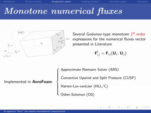
Monotone numerical fluxesPSfrag
Γij
Ωi
x, u
y, v
z, w
X, vX
Y, vY
Z, vZ
R(nG
ij)
nij
G
L
Several Godunov-type monotone 1st orderexpressions for the numerical fluxes vectorpresented in Literature
FIij = Fij(Ui, Uj)
Implemented in AeroFoam:
Approximate Riemann Solver (ARS)
Convective Upwind and Split Pressure (CUSP)
Harten-Lax-vanLeer (HLL/C)
Osher-Solomon (OS)
Un approccio “libero” alla moderna Aeroelasticita Computazionale

Introduction Structural system Aerodynamic system Coupling procedure Aeroelastic system Conclusions
High resolution numerical fluxes
Idea: combine a monotone 1st order numerical flux FIij (works fine near shocks)
and a 2nd order numerical flux FIIij (works fine in smooth flow regions) by means
of a flux-limiter function Φ
FHRij = FI
ij + Φ (FIIij − FI
ij ) = FIij + Aij ,
Implemented in AeroFoam
Lax-Wendroff (LW)
Jameson-Schmidt-Turkel (JST)
Remark
To build the antidissipative numerical fluxes vector Aij = Aij(Ui, Uj ; Ui∗ , Uj∗)numerical solutions Ui∗ and Uj∗ on extended cells Ωi∗ and Ωj∗ are also needed
Un approccio “libero” alla moderna Aeroelasticita Computazionale
Introduction Structural system Aerodynamic system Coupling procedure Aeroelastic system Conclusions
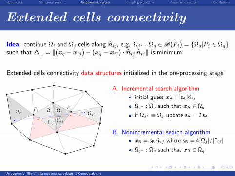
Extended cells connectivity
Idea: continue Ωi and Ωj cells along nij , e.g. Ωj∗ : Ωq ∈ B(Pj) = Ωq|Pj ∈ Ωqsuch that ∆⊥ = ‖(xq − xij)− (xq − xij) · nij nij‖ is minimum
Extended cells connectivity data structures initialized in the pre-processing stage
Ωi ΩjΩi∗ Ωj∗Pi
Pj
Γijnij
A. Incremental search algorithm
initial guess xA = sA bnij
Ωj∗ : Ωq such that xA ∈ Ωq
if Ωj∗ ≡ Ωj update sA = 2 sA
B. Nonincremental search algorithm
xB = sB bnij where sB = 4|Ωj |/|Γij |Ωj∗ : Ωq such that xB ∈ Ωq
Un approccio “libero” alla moderna Aeroelasticita Computazionale
Introduction Structural system Aerodynamic system Coupling procedure Aeroelastic system Conclusions
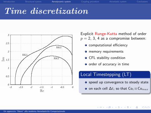
Time discretization
0
0.5
1
1.5
2
2.5
3
-3 -2.5 -2 -1.5 -1 -0.5 0
RK2
RK3
RK4
Re
Im
Explicit Runge-Kutta method of orderp = 2, 3, 4 as a compromise between:
computational efficiency
memory requirements
CFL stability condition
order of accuracy in time
Local Timestepping (LT)
speed up convergence to steady state
on each cell ∆ti so that Coi≡Comax
Un approccio “libero” alla moderna Aeroelasticita Computazionale
Introduction Structural system Aerodynamic system Coupling procedure Aeroelastic system Conclusions
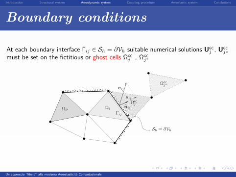
Boundary conditions
At each boundary interface Γij ∈ Sh = ∂Vh suitable numerical solutions UGCj , UGC
j∗must be set on the fictitious or ghost cells ΩGC
j , ΩGCj∗
Ωi
ΩGC
j
Ωi∗
ΩGC
j∗
Γij
nij
vij
Sh = ∂Vh
uij
Un approccio “libero” alla moderna Aeroelasticita Computazionale
Introduction Structural system Aerodynamic system Coupling procedure Aeroelastic system Conclusions
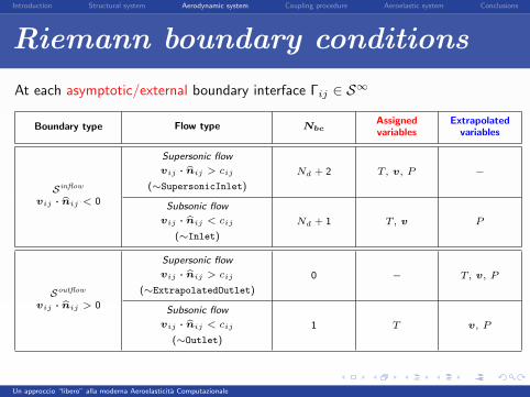
Riemann boundary conditions
At each asymptotic/external boundary interface Γij ∈ S∞
Boundary type Flow type NbcAssignedvariables
Extrapolatedvariables
Sinflow
vij · bnij < 0
Supersonic flow
vij · bnij > cij
(∼SupersonicInlet)
Nd + 2 T, v, P −
Subsonic flow
vij · bnij < cij
(∼Inlet)
Nd + 1 T, v P
Soutflow
vij · bnij > 0
Supersonic flow
vij · bnij > cij
(∼ExtrapolatedOutlet)
0 − T, v, P
Subsonic flow
vij · bnij < cij
(∼Outlet)
1 T v, P
Un approccio “libero” alla moderna Aeroelasticita Computazionale
Introduction Structural system Aerodynamic system Coupling procedure Aeroelastic system Conclusions
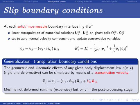
Slip boundary conditions
At each solid/impermeable boundary interface Γij ∈ Sb
linear extrapolation of numerical solutions UGCj , UGC
j∗ on ghost cells ΩGCj , ΩGC
j∗
set to zero normal velocity component and update conservative variables
vj = vj − (vj · nij) nij Etj = Et
j −1
2ρj |vj |2 +
1
2ρj |vj |2
Generalization: transpiration boundary conditions
The geometric and kinematic effects of any given body displacement law s(x, t)(rigid and deformative) can be simulated by means of a transpiration velocity:
vj = vj − (vj · nij) nij + Vn nij
Mesh is not deformed runtime (expensive) but only in the post-processing stage
Un approccio “libero” alla moderna Aeroelasticita Computazionale
Introduction Structural system Aerodynamic system Coupling procedure Aeroelastic system Conclusions
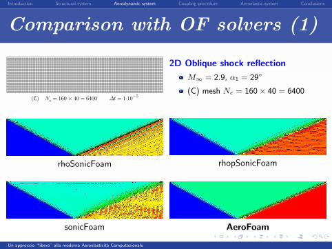
Comparison with OF solvers (1)
(C) Ne = 160 × 40 = 6400 ∆t = 1·10−5
2D Oblique shock reflection
M∞ = 2.9, α1 = 29
(C) mesh Ne = 160× 40 = 6400
rhoSonicFoam rhopSonicFoam
sonicFoam AeroFoam
Un approccio “libero” alla moderna Aeroelasticita Computazionale
Introduction Structural system Aerodynamic system Coupling procedure Aeroelastic system Conclusions
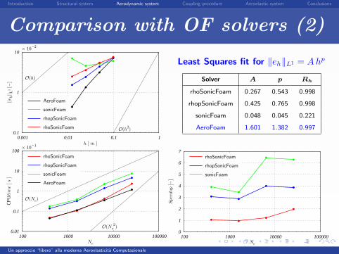
Comparison with OF solvers (2)
0.1
1
10
0.001 0.01 0.1 1
||eh||
L1 [−
]
h [ m ]
O(h)
O(h2)
× 10−2
AeroFoam
sonicFoam
rhopSonicFoam
rhoSonicFoam
Least Squares fit for ‖eh‖L1 = A hp
Solver A p Rh
rhoSonicFoam 0.267 0.543 0.998
rhopSonicFoam 0.425 0.765 0.998
sonicFoam 0.048 0.045 0.221
AeroFoam 1.601 1.382 0.997
0.01
0.1
1
10
100
100 1000 10000 100000
CPU
tim
e [
s]
Ne
O(Ne)
O(Ne
2)
× 10−1
rhoSonicFoam
rhopSonicFoam
sonicFoam
AeroFoam
0
1
2
3
4
5
6
7
100 1000 10000 100000
Speedup
[−]
Ne
rhoSonicFoam
rhopSonicFoam
sonicFoam
Un approccio “libero” alla moderna Aeroelasticita Computazionale
Introduction Structural system Aerodynamic system Coupling procedure Aeroelastic system Conclusions
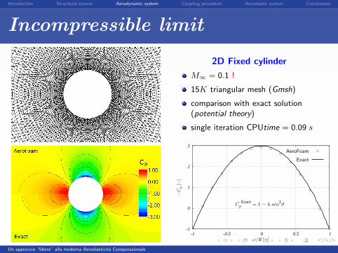
Incompressible limit
2D Fixed cylinder
M∞ = 0.1 !
15K triangular mesh (Gmsh)
comparison with exact solution(potential theory)
single iteration CPUtime = 0.09 s
-1
0
1
2
3
-1 -0.5 0 0.5 1
−C
p [−
]
x/R [−]
CpExact = 1 − 4 sin
2ϑ
AeroFoam
Exact
Un approccio “libero” alla moderna Aeroelasticita Computazionale
Introduction Structural system Aerodynamic system Coupling procedure Aeroelastic system Conclusions
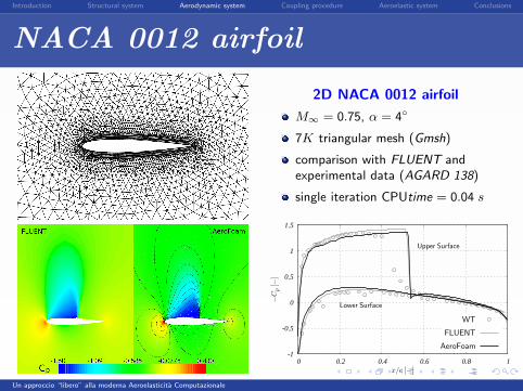
NACA 0012 airfoil
2D NACA 0012 airfoil
M∞ = 0.75, α = 4
7K triangular mesh (Gmsh)
comparison with FLUENT andexperimental data (AGARD 138)
single iteration CPUtime = 0.04 s
-1
-0.5
0
0.5
1
1.5
0 0.2 0.4 0.6 0.8 1
−C
p [−
]
x/c [−]
Upper Surface
Lower Surface
WT
FLUENT
AeroFoam
Un approccio “libero” alla moderna Aeroelasticita Computazionale
Introduction Structural system Aerodynamic system Coupling procedure Aeroelastic system Conclusions
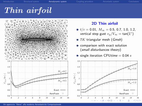
Thin airfoil
2D Thin airfoil
t/c = 0.01, M∞ = 0.5, 0.7, 1.0, 1.2,vertical step gust vg/V∞ = tan(1)
7K triangular mesh (Gmsh)
comparison with exact solution(small disturbances theory)
single iteration CPUtime = 0.04 s
0.4
0.6
0.8
1
1.2
1.4
1.6
0 2 4 6 8 10 12 14 16
CL
/α/2
π [−
]
τ [−]
M∞
=0.5
M∞
=0.7
Exact
AeroFoam
0.4
0.6
0.8
1
1.2
1.4
1.6
0 2 4 6 8 10 12 14 16
CL
/α/2
π [−
]
τ [−]
M∞
=1.2
M∞
=1.0
Exact
AeroFoam
Un approccio “libero” alla moderna Aeroelasticita Computazionale

Introduction Structural system Aerodynamic system Coupling procedure Aeroelastic system Conclusions
ONERA M6 wing (1)
b = 1.196 m
c r=
0.8
06
m
c t=
0.5
09
m
c
1
2
3
4
5
67
ΛLE = 30
ΛTE = 15.8
M∞ = 0.84
0.4
4c r
x
y
3D ONERA M6 wing
M∞ = 0.84, α = 3.06
350K tetrahedral mesh (GAMBIT)
comparison with FLUENT andexperimental data (AGARD 138)
single iteration CPUtime = 3.48 s
Un approccio “libero” alla moderna Aeroelasticita Computazionale

Introduction Structural system Aerodynamic system Coupling procedure Aeroelastic system Conclusions
ONERA M6 wing (2)
-1
-0.5
0
0.5
1
1.5
0 0.1 0.2 0.3 0.4 0.5 0.6 0.7 0.8 0.9 1
−C
p [−
]
x/c [−]
Upper Surface
Lower Surface
y/b = 0.20
WT
FLUENT
AeroFoam-1
-0.5
0
0.5
1
1.5
0 0.1 0.2 0.3 0.4 0.5 0.6 0.7 0.8 0.9 1
−C
p [−
]
x/c [−]
Upper Surface
Lower Surface
y/b = 0.95
WT
FLUENT
AeroFoam
Un approccio “libero” alla moderna Aeroelasticita Computazionale

Introduction Structural system Aerodynamic system Coupling procedure Aeroelastic system Conclusions
RAE A wing + body (1)
b = 0.457 m
cr = 0.228 m
ct = 0.076 m
L = 1.928 m
xw = 0.609 m
xb =0.760 m
c
Λc/2 = 30
x
Rb =Ro/2
ϕ
R(x) Ro = 0.076 m
xo = 0.508 m
1
2
3
4
5
6
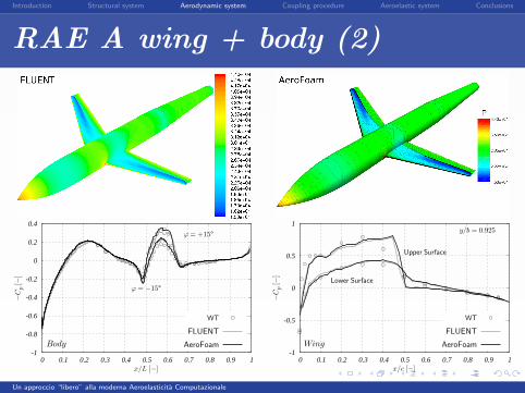
3D RAE A wing + body
M∞ = 0.9, α = 1
500K tetrahedral mesh (GAMBIT)
comparison with FLUENT andexperimental data (AGARD 138)
single iteration CPUtime = 4.52 s
Un approccio “libero” alla moderna Aeroelasticita Computazionale
Introduction Structural system Aerodynamic system Coupling procedure Aeroelastic system Conclusions
RAE A wing + body (2)
-1
-0.8
-0.6
-0.4
-0.2
0
0.2
0.4
0 0.1 0.2 0.3 0.4 0.5 0.6 0.7 0.8 0.9 1
−C
p [−
]
x/L [−]
ϕ = +15°
ϕ = −15°
Body
WT
FLUENT
AeroFoam
-1
-0.5
0
0.5
1
0 0.1 0.2 0.3 0.4 0.5 0.6 0.7 0.8 0.9 1
−C
p [−
]
x/c [−]
Upper Surface
Lower Surface
y/b = 0.925
Wing
WT
FLUENT
AeroFoam
Un approccio “libero” alla moderna Aeroelasticita Computazionale

Introduction Structural system Aerodynamic system Coupling procedure Aeroelastic system Conclusions
Aeroelastic interface
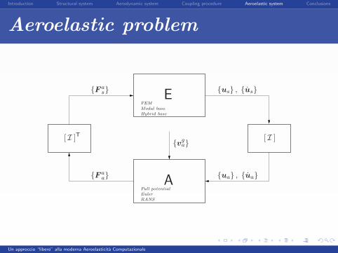
Target: closed loop connection between structural and aerodynamic sub-systems
Requirements:
connection between topologically different domains and non-conformal meshes
exact treatment of rigid motions
conservation of momentum and energy transfer (Lyapunov energetic stability)
ua = [ I ] usPrinciple of virtual work←−−−−−−−−−−−−→ F a
s = [ I ]T F aa
Reference test problem:
AGARD 445.6 wing
Structural mesh Ns = 121 nodes
Aerodynamic mesh Nba = 5506 triangles
Un approccio “libero” alla moderna Aeroelasticita Computazionale
Introduction Structural system Aerodynamic system Coupling procedure Aeroelastic system Conclusions
Linear interpolation
Ωj
xs, j1
xs, j2
xs, j3
s, j1
us, j2
us, j3
x⊥
a, i
ua, i
nj
n0, j
∆nj
us, j(x)
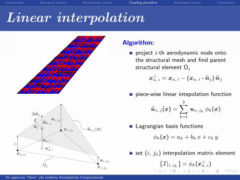
Algorithm:
project i-th aerodynamic node ontothe structural mesh and find parentstructural element Ωj
x⊥a, i = xa, i − (xa, i · bnj) bnj
piece-wise linear intepolation function
eus, j(x) =3X
k=1
us, jk φk(x)
Lagrangian basis functions
φk(x) = ak + bk x + ck y
set (i, jk) interpolation matrix element
[ I|i, jk ] = φk(x⊥a, i)
Un approccio “libero” alla moderna Aeroelasticita Computazionale
Introduction Structural system Aerodynamic system Coupling procedure Aeroelastic system Conclusions
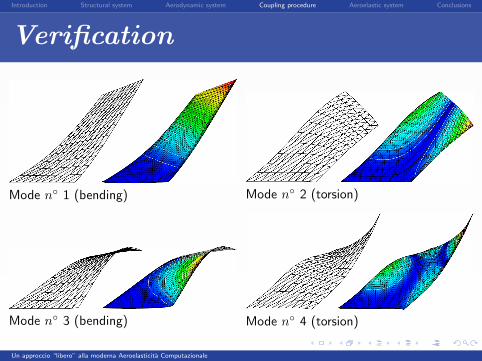
Verification
Mode n 1 (bending) Mode n 2 (torsion)
Mode n 3 (bending) Mode n 4 (torsion)
Un approccio “libero” alla moderna Aeroelasticita Computazionale
Introduction Structural system Aerodynamic system Coupling procedure Aeroelastic system Conclusions
Transpiration velocity (1)
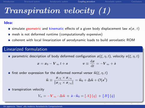
Idea:
simulate geometric and kinematic effects of a given body displacement law s(x, t)
mesh is not deformed runtime (computationally expensive)
coherent with local linearization of aerodynamic loads to build aeroelastic ROM
Linearized formulation
parametric description of body deformed configuration x(ξ, η, t), velocity v(ξ, η, t)
x = x0 − V ∞ t + s v ≡ dx
dt= −V ∞ + s
first order expression for the deformed normal versor bn(ξ, η, t)
bn ≡ x/ξ × x/η
‖x/ξ × x/η‖= bn0 + ∆bn +O(s2)
transpiration velocity
Vn = −V ∞ · ∆bn + s · bn0 = [ A ] q + [ B ] q
Un approccio “libero” alla moderna Aeroelasticita Computazionale
Introduction Structural system Aerodynamic system Coupling procedure Aeroelastic system Conclusions
Transpiration velocity (2)
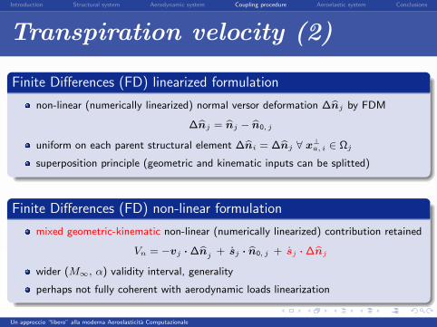
Finite Differences (FD) linearized formulation
non-linear (numerically linearized) normal versor deformation ∆bnj by FDM
∆bnj = bnj − bn0, j
uniform on each parent structural element ∆bni = ∆bnj ∀ x⊥a, i ∈ Ωj
superposition principle (geometric and kinematic inputs can be splitted)
Finite Differences (FD) non-linear formulation
mixed geometric-kinematic non-linear (numerically linearized) contribution retained
Vn = −vj · ∆bnj + sj · bn0, j + sj · ∆bnj
wider (M∞, α) validity interval, generality
perhaps not fully coherent with aerodynamic loads linearization
Un approccio “libero” alla moderna Aeroelasticita Computazionale

Introduction Structural system Aerodynamic system Coupling procedure Aeroelastic system Conclusions
Pitching NACA 64A010 airfoil
2D NACA 64A010 airfoil
M∞ = 0.796, ∆α = 0 ± 1.01,k = ωLa/V∞ = 0.202, La = c/2
3.5K triangular mesh (Gmsh)
comparison with Flo3xx andexperimental data (AGARD 702)
single iteration CPUtime = 0.02 s
-0.15
-0.1
-0.05
0
0.05
0.1
0.15
-1 -0.5 0 0.5 1
CL
[−]
α [ ° ]
Cycling to limit cycle
WT
Flo3xx
AeroFoam
Un approccio “libero” alla moderna Aeroelasticita Computazionale
Introduction Structural system Aerodynamic system Coupling procedure Aeroelastic system Conclusions
Aeroelastic problemreplacemen
E
A
FEM
Modal base
Hybrid base
Full potential
Euler
RANS
vg
a
ua , ua
us , us
F a
a
F a
s
[I ][I ]T
Un approccio “libero” alla moderna Aeroelasticita Computazionale
Introduction Structural system Aerodynamic system Coupling procedure Aeroelastic system Conclusions
Linearized aerodynamic loads
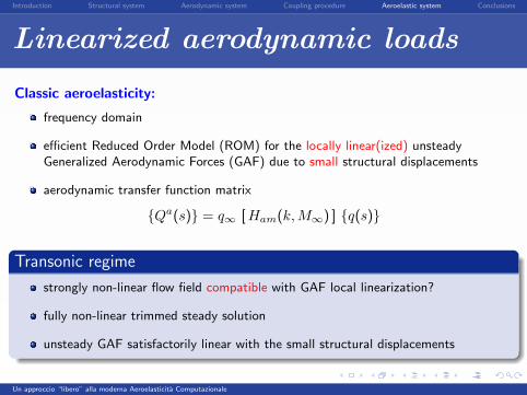
Classic aeroelasticity:
frequency domain
efficient Reduced Order Model (ROM) for the locally linear(ized) unsteadyGeneralized Aerodynamic Forces (GAF) due to small structural displacements
aerodynamic transfer function matrix
Qa(s) = q∞ [ Ham(k, M∞) ] q(s)
Transonic regime
strongly non-linear flow field compatible with GAF local linearization?
fully non-linear trimmed steady solution
unsteady GAF satisfactorily linear with the small structural displacements
Un approccio “libero” alla moderna Aeroelasticita Computazionale
Introduction Structural system Aerodynamic system Coupling procedure Aeroelastic system Conclusions
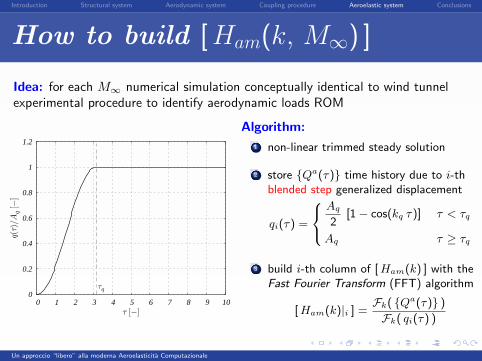
How to build [ Ham(k, M∞) ]
Idea: for each M∞ numerical simulation conceptually identical to wind tunnelexperimental procedure to identify aerodynamic loads ROM
0
0.2
0.4
0.6
0.8
1
1.2
0 1 2 3 4 5 6 7 8 9 10
q(τ)
/Aq [−
]
τ [−]
τq
Algorithm:
1 non-linear trimmed steady solution
2 store Qa(τ) time history due to i-thblended step generalized displacement
qi(τ) =
8<:Aq
2[1− cos(kq τ)] τ < τq
Aq τ ≥ τq
3 build i-th column of [ Ham(k) ] with theFast Fourier Transform (FFT) algorithm
[ Ham(k)|i ] =Fk( Qa(τ) )
Fk( qi(τ) )
Un approccio “libero” alla moderna Aeroelasticita Computazionale

Introduction Structural system Aerodynamic system Coupling procedure Aeroelastic system Conclusions
Block diagram
i = 1 i = 2 i = Nsi = Ns − 1
· · ·
· · ·
TRIM
GAFGAF GAFGAF
FFTFFT FFTFFT
ASSEMBLY COLUMNS
[ Ham(k) ]
Un approccio “libero” alla moderna Aeroelasticita Computazionale

Introduction Structural system Aerodynamic system Coupling procedure Aeroelastic system Conclusions
Structural model
AGARD 445.6 wing
laminated mahogany weakened model n3
Ground Vibration Test (GVT) data
[rmr] = 1 kg [rcr] ' 0 [rkr] = [rω20,ir]
only modes n1÷ 4 considered
FEM model set-up with a genetic optimizer(SciLab + Code Aster)
offset between experim. and numerical data
0
0.001
0.002
0.003
0.004
0.005
0.006
0.007
0.008
0.009
0
0.005
0.01
0.015
0.02
0.025
0.03
0.035
0
0.01
0.02
0.03
0.04
0.05
0.06
0
0.01
0.02
0.03
0.04
0.05
0.06
0.07
0.08
0.09
Error mode n
1 Error mode n
2 Error mode n
3 Error mode n
4
ef1= 0.3% ef2
= 2.9% ef3= 4.1% ef4
= 2.1%
Un approccio “libero” alla moderna Aeroelasticita Computazionale
Introduction Structural system Aerodynamic system Coupling procedure Aeroelastic system Conclusions
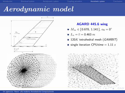
Aerodynamic model
b
cr
ct
c
1
2
3
4
Λc/4
M∞
cr/4
x
y
NACA 65A004
AGARD 445.6 wing
M∞ ∈ [ 0.678, 1.141 ], α0 = 0
La = c = 0.463 m
120K tetrahedral mesh (GAMBIT)
single iteration CPUtime = 1.11 s
Un approccio “libero” alla moderna Aeroelasticita Computazionale
Introduction Structural system Aerodynamic system Coupling procedure Aeroelastic system Conclusions
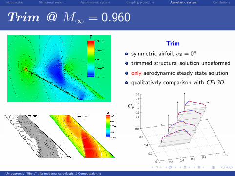
Trim @ M∞ = 0.960
Trim
symmetric airfoil, α0 = 0
trimmed structural solution undeformed
only aerodynamic steady state solution
qualitatively comparison with CFL3D
0 0.2 0.4 0.6 0.8 1 1.2
0
0.2
0.4
0.6
0.8
-0.4
-0.2
0
0.2
0.4
0.6
Cp
Un approccio “libero” alla moderna Aeroelasticita Computazionale
Introduction Structural system Aerodynamic system Coupling procedure Aeroelastic system Conclusions
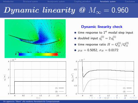
Dynamic linearity @ M∞ = 0.960
Dynamic linearity check
time response to 1st modal step input
doubled input q(2)1 = 2 q
(1)1
time response ratio H = Q(1)11 /Q
(2)11
µH = 0.5052, σH = 0.0172
0
1
2
3
4
0 0.5 1 1.5 2 2.5 3
q1 [m
]
τ [−]
× 10−3
(1)
(2)-2
-1.5
-1
-0.5
0
0 0.5 1 1.5 2 2.5 3
Q11
[m
2]
τ [−]
× 10−1
(1)
(2)
Un approccio “libero” alla moderna Aeroelasticita Computazionale
Introduction Structural system Aerodynamic system Coupling procedure Aeroelastic system Conclusions
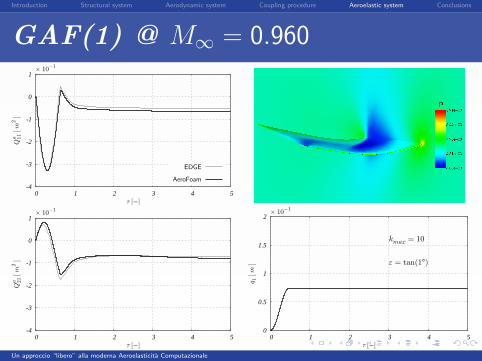
GAF(1) @ M∞ = 0.960
-4
-3
-2
-1
0
1
0 1 2 3 4 5
Q11
[m
2]
τ [−]
a
× 10−1
EDGE
AeroFoam
-4
-3
-2
-1
0
1
0 1 2 3 4 5
Q21
[m
2]
τ [−]
a
× 10−1
0
0.5
1
1.5
2
0 1 2 3 4 5
q1 [m
]
τ [−]
kmax = 10
ε = tan(1°)
× 10−1
Un approccio “libero” alla moderna Aeroelasticita Computazionale
Introduction Structural system Aerodynamic system Coupling procedure Aeroelastic system Conclusions
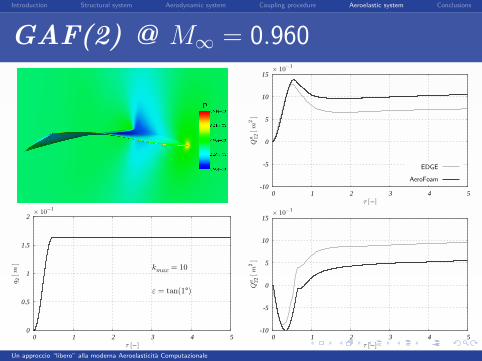
GAF(2) @ M∞ = 0.960
-10
-5
0
5
10
15
0 1 2 3 4 5
Q12
[m
2]
τ [−]
a
× 10−1
EDGE
AeroFoam
0
0.5
1
1.5
2
0 1 2 3 4 5
q2 [m
]
τ [−]
kmax = 10
ε = tan(1°)
× 10−1
-10
-5
0
5
10
15
0 1 2 3 4 5
Q22
[m
2]
τ [−]
a
× 10−1
Un approccio “libero” alla moderna Aeroelasticita Computazionale

Introduction Structural system Aerodynamic system Coupling procedure Aeroelastic system Conclusions
[ Ham(k) ] @ M∞ = 0.960
-4
-3
-2
-1
0
1
0 0.2 0.4 0.6 0.8 1
Ham
,11
[m
]
k [−]
-10
-5
0
5
10
0 0.2 0.4 0.6 0.8 1
Ham
,12
[m
]
k [−]
EDGE
Literature
AeroFoam
Re
Im
-4
-3
-2
-1
0
1
0 0.2 0.4 0.6 0.8 1
Ham
,21
[m
]
k [−]
-10
-5
0
5
10
0 0.2 0.4 0.6 0.8 1
Ham
,22
[m
]
k [−]
Un approccio “libero” alla moderna Aeroelasticita Computazionale
Introduction Structural system Aerodynamic system Coupling procedure Aeroelastic system Conclusions
Flutter analysis (1)
0
20
40
60
80
100
200 250 300 350 400
f [
Hz
]
V∞
[ m/s ]
VF
-0.4
-0.3
-0.2
-0.1
0
0.1
0.2
200 250 300 350 400
g [−
]
V∞
[ m/s ]
VF
Mode n° 1
Mode n° 2
Mode n° 3
Mode n° 4
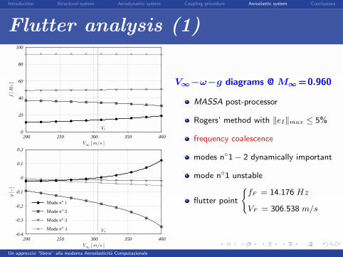
V∞−ω−g diagrams @ M∞ =0.960
MASSA post-processor
Rogers’ method with ‖eI‖max ≤ 5%
frequency coalescence
modes n1− 2 dynamically important
mode n1 unstable
flutter point
(fF = 14.176 Hz
VF = 306.538 m/s
Un approccio “libero” alla moderna Aeroelasticita Computazionale
Introduction Structural system Aerodynamic system Coupling procedure Aeroelastic system Conclusions
Flutter analysis (2)
0.3
0.4
0.5
0.6
0.7
0.8
0.6 0.7 0.8 0.9 1 1.1 1.2
Iω [−
]
M∞
[−]
Experimental
CFL3D
EDGE
FLUENT
AeroFoam
0.2
0.3
0.4
0.5
0.6
0.7
0.6 0.7 0.8 0.9 1 1.1 1.2
Iv [−
]
M∞
[−]
Experimental
CFL3D
EDGE
FLUENT
AeroFoam
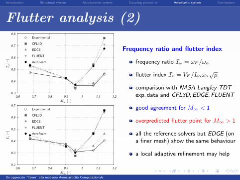
Frequency ratio and flutter index
frequency ratio Iω = ωF /ωα
flutter index Iv = VF /Lαωα√
µ
comparison with NASA Langley TDTexp. data and CFL3D, EDGE, FLUENT
good agreement for M∞ < 1
overpredicted flutter point for M∞ > 1
all the reference solvers but EDGE (ona finer mesh) show the same behaviour
a local adaptive refinement may help
Un approccio “libero” alla moderna Aeroelasticita Computazionale
Introduction Structural system Aerodynamic system Coupling procedure Aeroelastic system Conclusions
Conclusions and future work
Conclusions:
a toolbox of free software (Code Aster+OpenFOAM) for CA has been developed
satisfactory agreement with similar toolbox of commercial software (NAEMO CFD)
computational cost still too high: very difficult to implement a fully implicit timeintegration scheme in OpenFOAM (lduMatrix class, maybe in OpenFOAM 1.5)
. . . and future work:
aeroservoelastic applications: flutter suppression active control design (BACT wing)
runtime mesh deformation: new face swapping moving algorithm
tackle industrial aeroelastic 3D problems (e.g. Piaggio P-180)
Un approccio “libero” alla moderna Aeroelasticita Computazionale