ultrasonic flow meter diagnostics and the impact of . · pdf filekrohne: ultrasonic flow meter...

Krohne: Ultrasonic flow meter diagnostics and the impact of fouling. page 1 of 22 AGA 2011 Operations Conference

Ultrasonic flow meter diagnostics and the impact of fouling.

Jan G. Drenthen, Marcel Vermeulen, Martin Kurth & Hilko den Hollander Krohne Oil & Gas

1. Introduction Over the past decade, Ultrasonic flow meters have gained a wide acceptance. Main reasons for this are the high repeatability in combination with zero pressure loss and extensive diagnostic features. Over the years, meters with different path configurations have been put into the market, each of them trying to obtain the highest accuracy. Many of them show (often after multipoint linearization) almost perfect straight lines with errors close to the repeatability of the lab. However, for a user it is not only important to know how good his meter is at the lab; far more important is the assurance that the accuracy after installation in the field is not deteriorating over time. Major factors affecting the performance of a meter installed in the field are corrosion and fouling. This is not only a problem for ultrasonic meters, but it will affect every flow meter installed. The great virtue of ultrasonic flow meters in contrast to all other meters, are their huge diagnostic capabilities. Especially the newly designed ultrasonic flowmeters using reflecting paths instead of the old fashioned straight path designs, are capable of even detecting very slight changes in the conditions at the pipe wall. While there are multiple papers on the performance in calibration laboratories, the impact that fouling and corrosion can have on the performance of an ultrasonic meter is less known. One of the first papers describing the impact of installation conditions was that of Rick Wilsack and Huib Dane [2]. Recently James Witte has presented a paper including also the impact that it has on the flow velocity profile [5]. The present paper focuses on the impact of fouling and corrosion and addresses:

the design considerations the ways to detect the various categories of fouling the tests performed with dirty meters the impact of honed versus corroded upstream pipes. the impact of corrosion of the reflecting surface.

Next to this, a first order correction is presented, amongst others based on the information gathered from the reflecting paths.

2. Ice berg specifications When comparing the specifications of different ultrasonic flow meters, all manufacturers show similar specifications, this despite the obvious differences in their designs: :

Uncertainty

≤ ±0.5% of measured value, uncalibrated

≤ ±0.2% of measured value, high-pressure flow calibrated (relative to calibration laboratories)

≤ ±0.1% of measured value, calibrated and linearized

Repeatability ≤ ±0.1% Table 1: The ice berg specifications

What all of the different manufacturers do not mention in their datasheet are:

1. the transferability of the calibration curve obtained under almost ideal conditions in the calibration facility (see figure 1) to the actual conditions in the field (see figure 2); the installation effects.

2. The impact of fouling and corrosion on the meter performance.


Figure 1: Ideal conditions at test rig (courtesy of TCC) Figure 2: Actual conditions in the field

Figure 3: A clean ultrasonic meter at a calibration. Figure 4: A dirty meter during visual inspection

The transferability of the calibration curve to the field has been investigated, amongst others by T. Grimley (see ref. [4]) and is for the conventional direct path meter types, typical in the order of 0,5 %. The Altosonic V12 has been specifically designed to minimize the impact of installation effects. As a result of that this sensitivity has been reduced to a value < 0.2% (see ref. [2]). Whereas during flow calibration the meter is clean, after several months in operation, the meter might be contaminated. The introduced additional uncertainty as a result of this, can easily reach 0,5%, the same magnitude as that of the installation effects. Including this in the equation results in a total uncertainty which is much larger than those stated in the datasheets.


So in effect, the specifications shown in the manufacturer’s datasheets are nothing more than Ice berg specifications; the real specifications are hidden below the surface, meaning:

The sensitivity to installation effects The impact of fouling and corrosion.

Table 2: Total uncertainty estimation

In order to reduce the total uncertainty, the impact of both the installation effect as well as the sensitivity to contamination has to be reduced. These have been the prime targets in the development of the Altosonic V12 ultrasonic gas flow meter.

3. Meter design As a function of their path configuration, presently 3 different types can be distinguished (see figure 5):

Conventional parallel chord designs (A) Conventional reflective chord designs (B) The (patented) Krohne V-12 path arrangement (C)

A B C

Figure 5: Conventional parallel chord design (A), conventional reflective chord design (B) & the Krohne V12 design (C)

Looking at the conventional meter designs, it must be concluded that despite some occasionally lucky shots, all of them are affected by highly distorted flows and / or fouling. Reasons for this are:

o The conventional parallel chord designs are able to measure close to the pipe wall but do not reflect and lack therefore the interrogation of the pipe wall.


o The conventional reflective chord design could be able to measure wall built-up, but its triangle shaped paths cannot get closer to the wall than the 0.5R position; This position is too far away to effectively deal with changes in the flow profile close to the wall.

The optimal solution to overcome these issues is a combination of both technologies: the KROHNE ALTOSONIC V12 design. (see figure 6)

Figure 6: Krohne V12 path configuration. In this configuration:

o There are 5 horizontal paths and one vertical aligned path. o Each path consists of 2 chords formed into a single V-bounce (in total the meter is equipped with

12 chords, all with a single V shape). o The vertical reflecting path is used solely to detect the presence of contamination liquid layers on

the bottom of the pipe. o All paths are reflecting whereby four of them use small acoustic mirrors at the opposite side of the

pipe. As a result, the meter is designed to achieve both the highest accuracy and be able to detect fouling.

4. Variations in fouling

Looking at fouling, one of the main problems is the variety at which it occurs. In figures 7 to 9 some examples of (excessive) fouling as encountered in real situations are presented. Figure 7 is the result of a production problem, figure 8 is an example of an off-shore installation and figure 9 is an on-shore installation.

Figure 7, fouling as a flow on the bottom of the pipe. Figure 8, fouling intermittently stuck to the pipe wall


Looking at the impact that fouling can have on ultrasonic meters, it can be classified into 5 categories. Each of them may affect the measurement in a different way. These categories are:

1. Fouling as a small flow on the bottom of the pipe. (water, condensate) 2. Fouling intermittently sticking to the pipe wall. (wax, gunk) 3. Fouling as an evenly distributed coating on the inside of the pipe. (black powder, corrosion) 4. Fouling as dirt build-up on the transducers (especially on those facing upstream). (wax, tar) 5. Fouling as liquid build-up in the transducer pockets. (water, condensate)

For ultrasonic flow meters the major effects of fouling on the measurement are:

A reduction of the cross sectional area. An increased wall roughness. The shortening of the acoustic path length. The attenuation of the acoustic signal through the reduction of the reflection coefficient. The absorbance of the ultrasonic signal due to the layer of fouling on the transducer. Increased cross talk when liquid is present in the transducer pockets.

5. Testing at Lintorf In July 2010 extensive testing have been done at the E-ON Ruhrgas test facility in Lintorf using two 6” ALTOSONIC V12 meters in series (see figure 10).

Figure 10, two 6” Altosonic V12 meters in series at Lintorf

Figure 9, fouling evenly distributed over the pipe wall


The Lintorf facility is one of the most flexible facilities available. The pressure can be varied between 8 and 45 bar and flows can be generated up to 40.000 m3N/h (in summer; winter up to 100.000 m3N/h). As reference meters there is a series of 5 parallel runs of orifices as well as a turbine meter (see figure 11). After finishing the tests, an Altosonic V12 meter has been installed as a permanent reference. For the testing described in this paper the repeatability was the most important item rather than the absolute error and / or the shape of the error curve. Figure 11 Layout of the Lintorf facility.

5.1. Test program

The tests were done at the end of July under hot and changing weather conditions. As a result of this stratified flow profiles occurred at - lower flow velocities, affecting the repeatability which manifested itself in a somewhat larger spread in the baselines than usual. However, the repeatability assessed during the two weeks of testing still remained mostly within the order of 0.1% to 0.15% only at the lower flow velocities below approximately 4 m/s the uncertainty increased. During the tests all the above mentioned types of fouling have been investigated with additional tests on corrosion. Investigated were:

1. Fouling on the bottom. 2. Fouling intermittently sticking on the pipe wall. 3. Fouling of evenly distributed inside the pipe. 4. Fouling on the transducers. 5. Liquid contamination in the transducer pockets. Additional: 6. Reflection on rough (corroded) surfaces 7. Honed and corroded upstream pipes

To create the fouling a variety of products such as water, oil, putty and anti-seize lubricating compound were applied.

5.2. Fouling on the bottom of the pipe

Fouling on the bottom of the pipe can be detected by using a vertical reflecting path. The stability and ability to detect this depends on the viscosity, the density of the fluid at the bottom of the meter and the gas in the meter, as well as the flow velocity. The behavior of the bottom layer depends on both the fluid properties as well as the pressure and flow velocity of the gas. A detailed description of the various patterns is presented in [3]. To simulate the bottom fouling and to test the sensitivity of the diagnostic detection, an approximately 4 to 6 cm wide and relatively thin layer of “never-seize regular grade anti-seize and lubricating compound” -further to be referred to as “grease”- was applied over the whole length of both the inlet spool and the meter. Measuring the thickness proved not to be an easy task and an assessment was made using calipers and by weighing the amount of grease applied. Based on these the thickness was estimated as an average layer of about 0.5 mm with peaks of 2 mm. (see figure 12). However the uncertainty of this measurement,


especially that of the average thickness, with grease sticking to the caliper is quite large. Using the change in acoustic path length is much easier and also much more accurate. As a result for all this and all the remaining tests, the speed of sound measurement was used for assessing the thickness.

Figures 12 bottom fouling

For this type of fouling, the expected most important diagnostic parameters are:

o The change in the speed of sound of the path reflecting on the bottom of the pipe, path 6. o The reflection coefficient of this path. o The change in the standard deviation of both the velocity as the SOS.

Due to the fact that there were some rumors that bottom fouling could also be detected by the change in the flow velocity profile alone, this was checked as well and presented in figure 13.

Figure 13, Flow velocity profile with and without bottom fouling (on the right side) Looking at figure 13, it is evident that the change in the flow velocity profile is minimal and absolutely not enough to be used as an indicator; only when there is an extreme spilling it might be used. The second indicator is the reflection coefficient, measured as a change in the signal strength. This is presented in figure 14.

-12.0%

-10.0%

-8.0%

-6.0%

-4.0%

-2.0%

0.0%

2.0%

4.0%

6.0%

8.0%

-1.00 -0.80 -0.60 -0.40 -0.20 0.00 0.20 0.40 0.60 0.80 1.00


Figure 14, change in the reflection coefficient Although stable, the change in the reflection coefficient on such a small layer of grease is less than 1 dB. The same change in signal strength occurs when the pressure changes some 10%. On itself this is insufficient to draw conclusions from and this parameter is therefore only to be used in combination with other parameters. The change in standard deviation in the flow velocity and that of the SOS are useful parameters for indicating changes in the hydraulic roughness. With fluid contamination on the bottom, this occurs when the fluid surface changes from smooth to wavy. In figure 15 the standard deviation is shown of both the path reflecting at the bottom (path 6) and that on the side, which is unaffected by the fouling on the bottom (path 3).

Figure 15, Standard deviation of path 3 & 6

In this picture can be seen, that ripples are formed at higher flow velocities leading to a larger fluctuation in the SOS. Also, the thickness of the layer as well as its viscosity will impact the result. Again: on itself this parameter alone is insufficient to draw conclusions from but can be very useful in combination with other parameters.

60.0

62.0

64.0

66.0

68.0

70.0

72.0

74.0

0.00 5.00 10.00 15.00 20.00 25.00 30.00 35.00

GAINBA6GAINBA6GAINBA1GAINBA2GAINBA3GAINBA4GAINBA5GAINBA6

Signal strength with and without

bottom fouling

60.0

62.0

64.0

66.0

68.0

70.0

72.0

74.0

0.00 5.00 10.00 15.00 20.00 25.00 30.00 35.00

GAINBA6GAINBA6GAINBA1GAINBA2GAINBA3GAINBA4GAINBA5GAINBA6

Signal strength with and without

bottom fouling

0.00

0.05

0.10

0.15

0.20

0.25

0.30

0.35

0.40

0.00 5.00 10.00 15.00 20.00 25.00 30.00 35.00

SDCh_SoS[3]SDCh_SoS[6]SDCh_SoS[3]SDCh_SoS[6]SDCh_SoS[1]SDCh_SoS[2]SDCh_SoS[3]SDCh_SoS[4]SDCh_SoS[5]SDCh_SoS[6]

Path 3

Path 6

0.00

0.05

0.10

0.15

0.20

0.25

0.30

0.35

0.40

0.00 5.00 10.00 15.00 20.00 25.00 30.00 35.00


Path 3

Path 6

0.00

0.05

0.10

0.15

0.20

0.25

0.30

0.35

0.40

0.00 5.00 10.00 15.00 20.00 25.00 30.00 35.00


Path 3

Path 6


Clearly in this case, the absolute value of the speed of sound is the most important and direct parameter. In figure 16, the speed of sound ratio’s of all the acoustic paths are shown.

Figure 16, Speed of sound ratio’s In this figure it can be seen that the speed of sound of path 6, the diagnostic path reflecting on the bottom of the pipe has shifted approximately 0.2 % in respect to the other paths. Calculated on the shift in the speed of sound, the average thickness of the bottom layer was 0.3 mm; somewhat lower than assessed by the mechanical measurement. As a first order correction, based on the blockage of the cross sectional area, such a layer results in a total reduction of the cross sectional area of 0.12%. In figure 17, the calibration results of both the “clean” meter as well as that with bottom fouling are shown. From these, it is clear that the first order correction is in close agreement with the measured offset.

Bottom fouling

-0.20

0.00

0.20

0.40

0.60

0.80

1.00

0.00 5.00 10.00 15.00 20.00 25.00 30.00 35.00

m/s

% e

rror

base downstreambottem fouling

Figure 17 Calibration curves of both the clean meter and with bottom fouling

5.3. Fouling, intermittently sticking to the pipe wall.

The fouling intermittently stuck to the wall is slowly moved forward by the gas through the pipe. How quickly it moves is depends on the gas flow velocity, its density and the characteristics of the fouling itself. In practice it is not possible to predict when it will be present at a certain position in the pipe but it is certain that eventually every single point in the pipe will be affected over time.

First order correction

SOS comparison; bottom fouling

-0.30%

-0.20%

-0.10%

0.00%

0.10%

0.20%

0.30%

0.40%

0.50%

0.00 5.00 10.00 15.00 20.00 25.00 30.00 35.00

m/s

% d

iffer

ence


For the tests, generous portions of grease were randomly applied to the pipe wall of both the inlet spool as the meter (see figures 18a &18b).

Figures 18: Fouling sticking intermittently to the pipe wall.

Using reflective paths, this type of fouling shows an irregular behavior in the speed of sound readings as well as the AGC readings of the various paths. Also the average wall roughness is affected, resulting in a changing velocity profile. For this type of fouling, the expected most important diagnostic parameters are:

o The over time erratic changes in the speed of sound of the reflecting paths. o The variations in the signal strength. o The possible change in the flow velocity profile. o The changes standard deviation of the various paths.

In figure 19, the change in the flow velocity profile is shown at two flow velocities (solid clines without fouling; striped line with fouling).

Figure 19, change in flow velocity with and without intermittent fouling. From this figure, it can be seen that, as expected, the flow velocity profile is somewhat sharper. The change in itself however, is insufficient to be used as a sole indicator but can be very useful in combination with other parameters. A handy way to look at changes in the speed of sound is by looking at the so-called “footprint”. This footprint is based on the ratios of the speed of sound of the various paths. The figure is created by

-12.0%

-10.0%

-8.0%

-6.0%

-4.0%

-2.0%

0.0%

2.0%

4.0%

6.0%

8.0%

-1.00 -0.80 -0.60 -0.40 -0.20 0.00 0.20 0.40 0.60 0.80 1.00

#N/B15.537.77#N/B#N/B#N/B15.477.75#N/B#N/B#N/B#N/B#N/B#N/B#N/B

With fouling

-12.0%

-10.0%

-8.0%

-6.0%

-4.0%

-2.0%

0.0%

2.0%

4.0%

6.0%

8.0%

-1.00 -0.80 -0.60 -0.40 -0.20 0.00 0.20 0.40 0.60 0.80 1.00

#N/B15.537.77#N/B#N/B#N/B15.477.75#N/B#N/B#N/B#N/B#N/B#N/B#N/B

With fouling


dividing the SOS of path 1 / the SOS of path 2; the SOS of path 1 / the SOS of path 3; the SOS of path 1 / the SOS of path 4, etcetera. By comparing this with that of the undisturbed situation, in a quick manner problems can be found. In figure 20, the footprint of the undisturbed situation (solid lines) with that of the intermittently fouling (striped) is shown.

Figure 20, SOS footprint with and without intermittent fouling From this figure can be seen that path 3 has shifted some 0.2% and path 6 almost 0.1%. In figure 21, the relative changes in speed of sound for the 6 acoustic paths as a function of the flow velocity is shown.

Figure 21, Speed of sound for the 6 acoustic paths as a function of the flow velocity

From this it can be seen that the rate of change is not stable and changes over time as a function of the gas velocity. As a result, also the errors are not stable.

Fouling, intermittendly sticking to the pipewall

-0.05%

-0.04%

-0.03%

-0.02%

-0.01%

0.00%

0.01%

0.02%

0.03%

0.04%

0.05%

0.00 5.00 10.00 15.00 20.00 25.00 30.00 35.00

m/s

-0.250%

-0.200%

-0.150%

-0.100%

-0.050%

0.000%

0.050%

0.100%

0.150%

0.200%

0.250%

SOS12 SOS13 SOS14 SOS15 SOS23 SOS24 SOS25 SOS34 SOS35 SOS45 SOS16 SOS26 SOS36 SOS46 SOS56

#N/B15.527.863.92#N/B#N/B15.557.833.88#N/B#N/B#N/B#N/B#N/B#N/B


Fouling, intermittendly sticking to the wall

-0.20

0.00

0.20

0.40

0.60

0.80

1.00

0.00 5.00 10.00 15.00 20.00 25.00 30.00 35.00

m/s

base downstreamintermittently fouling

Figure 22: error curve with fouling sticking intermittently to the pipe wall

Despite the relatively small changes in the speed of sound, the impact on the error curve is significant (see fig 22). The first order correction based on just a single measurement in time is not sufficient to predict the error. Clearly in these situations trending is a necessity so that the full scale of the fouling can be determined. Certainly this type of fouling will be further investigated.

5.4. Fouling which is as an evenly distributed coating on the inside of the pipe This type of fouling is more difficult to detect and also here trending is necessary. With the wall build-up being identical for all the paths, the relative impact for paths of different lengths will be different. With increasing build-up there will be an increasing deviation in the average speed of sound for the paths with different path lengths. When a gas chromatograph is present, also the absolute speed of sound can be calculated and a more precise estimation of the thickness of the layer can be made. The build-up affects also the wall roughness, which results in a gradual changing flow velocity profile. Dependent on the path position, there are differences in how much the paths are affected:

the path through the middle of the pipe is the most sensitive to profile changes (and therefore essential in the detection)

in contrast to this, the paths on half radius chords are highly immune to wall roughness changes. The impact on the path close to the wall is very much dependent on its relative position, but

different from the others. As a result, the changes in the flow velocity profile can be detected by monitoring the trending the flow velocity ratios of the paths close to the pipe wall and the path through the middle of the pipe in respect to the half radius paths. Important (trending) parameters to detect this sort of fouling are:

the change in the flow velocity profile the change in the reflection coefficient the standard deviation in the SOS and flow velocity the ratio between the speed of sound of paths with different path lengths

To find out how the meter reacts to extreme fouling, extensive layers of grease were applied (see figure 23).



Figure 23 extreme evenly coated fouling. At first, in figure 24, the change in the flow velocity profile is shown.

Figure 24, Evenly fouling, the change in the velocity profile

Figure 24, evenly fouling, change in the flow velocity profile From this figure, it can be seen that, due to the increased roughness, the flow velocity profile is somewhat sharper. The change in itself is insufficient to be used as a sole indicator but can be very useful in combination with other parameters. The second item is the change in reflection coefficient. These are presented in figure 25.

-14.0%

-12.0%

-10.0%

-8.0%

-6.0%

-4.0%

-2.0%

0.0%

2.0%

4.0%

6.0%

8.0%

-1.00 -0.80 -0.60 -0.40 -0.20 0.00 0.20 0.40 0.60 0.80 1.00

#N/B15.52#N/B#N/B#N/B#N/B15.55#N/B#N/B#N/B#N/B#N/B#N/B#N/B#N/B


Figure 25, evenly fouling, change in the reflection coefficient From this figure, it can be seen that the change in reflection coefficient of path 3 is more than twice of that of path 6. Also, the thickness of the fouling on path 3 is approximately twice that of path 6 (0.6 mm. versus 0.3 mm). As a first estimation therefore, the ripples in the fouling of path 3 are twice as deep as those that of path 6. If that is the case, the standard deviation of path 3 must be much larger than that of path 6. These are shown in figure 26.

Figure 26, evenly fouling, change in the standard deviation in the SOS Here it can be seen, that the change in the standard deviation of path 3 is much larger than that of path 6, which seems not to be affected at all. A further and more detailed analysis of this phenomenon is only possible when trending data are available. Next to the standard deviation in the speed of sound, the absolute speed of sound is an important parameter. In case there is no reference for the absolute value of the speed of sound to compare with, the ratio’s of the various paths compared with the average value of these can be monitored. These are presented in figure 27.

60.0

62.0

64.0

66.0

68.0

70.0

72.0

74.0

76.0

0.00 5.00 10.00 15.00 20.00 25.00 30.00 35.00

GAINAB3GAINAB6GAINAB3GAINAB6GAINAB1GAINAB2GAINAB3GAINAB4GAINAB5GAINAB6

Change in signal strength on the reflecting paths

60.0

62.0

64.0

66.0

68.0

70.0

72.0

74.0

76.0

0.00 5.00 10.00 15.00 20.00 25.00 30.00 35.00


60.0

62.0

64.0

66.0

68.0

70.0

72.0

74.0

76.0

0.00 5.00 10.00 15.00 20.00 25.00 30.00 35.00


Change in signal strength on the reflecting paths

Sta

ndar

d de

viat

ion

0.00

0.05

0.10

0.15

0.20

0.25

0.30

0.35

0.40

0.45

0.50

0.00 5.00 10.00 15.00 20.00 25.00 30.00 35.00


Change in the SOS standard deviation of the reflecting paths

Sta

ndar

d de

viat

ion

0.00

0.05

0.10

0.15

0.20

0.25

0.30

0.35

0.40

0.45

0.50

0.00 5.00 10.00 15.00 20.00 25.00 30.00 35.00


Change in the SOS standard deviation of the reflecting paths


Figure 27, evenly fouling, relative changes in the speed of sound.

Based on the shifts in the SOS, an estimation of the average thickness of the fouling and the resulting reduction of the cross sectional area can be made. In this case, the calculated error due to the reduction of the cross sectional area is 0.5%; slightly higher than the measured value (see figure 28).

Evenly fouling

-0.20

0.00

0.20

0.40

0.60

0.80

1.00

0.00 5.00 10.00 15.00 20.00 25.00 30.00 35.00

base downstreamevenly fouling

Figure 28: error curve at evenly distributed fouling.

5.5. Dirt build-up on the transducers

For the tests, two different types of “dirt” were applied: one with tape and one with grease covering the top of the transducer (see figures 29).


Relative SOS at evenly fouling

-0.10%

-0.05%

0.00%

0.05%

0.10%

0.15%

0.20%

0.00 5.00 10.00 15.00 20.00 25.00 30.00 35.00

m/s


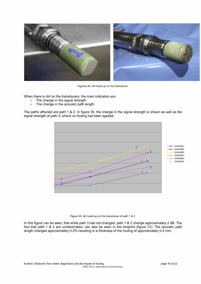
Figures 29: dirt build-up on the transducer.

When there is dirt on the transducers, the main indicators are:

o The change in the signal strength. o The change in the acoustic path length.

The paths affected are path 1 & 2. In figure 30, the change in the signal strength is shown as well as the signal strength of path 3, where no fouling has been applied.

Figure 30: dirt build-up on the transducer of path 1 & 2. In this figure can be seen, that while path 3 has not changed, path 1 & 2 change approximately 2 dB. The fact that path 1 & 2 are contaminated, can also be seen in the footprint (figure 31). The acoustic path length changes approximately 0.2% resulting in a thickness of the fouling of approximately 0.4 mm.

60.0

62.0

64.0

66.0

68.0

70.0

72.0

74.0

76.0

0.00 5.00 10.00 15.00 20.00 25.00 30.00 35.00

GAINAB1GAINAB2GAINAB3GAINAB1GAINAB2GAINAB3GAINAB1GAINAB2GAINAB3GAINAB4GAINAB5GAINAB6

3

1

2

2

1

60.0

62.0

64.0

66.0

68.0

70.0

72.0

74.0

76.0

0.00 5.00 10.00 15.00 20.00 25.00 30.00 35.00


60.0

62.0

64.0

66.0

68.0

70.0

72.0

74.0

76.0

0.00 5.00 10.00 15.00 20.00 25.00 30.00 35.00


3

1

2

2

1


Figure 31: Footprint, dirt build-up on the transducer of path 1 & 2 The impact on the error curve is show in figure 32. It can clearly be seen, that there is hardly any effect on the error curve and all curves are within the repeatability of the test site.

Dirt on the transducers

-0.40

-0.20

0.00

0.20

0.40

0.60

0.80

1.00

0.00 5.00 10.00 15.00 20.00 25.00 30.00 35.00

baselinewith tapeanti-seize

Figure 32: impact of dirt on the transducers.

-0.250%

-0.200%

-0.150%

-0.100%

-0.050%

0.000%

0.050%

0.100%

0.150%

0.200%

0.250%

SOS12 SOS13 SOS14 SOS15 SOS23 SOS24 SOS25 SOS34 SOS35 SOS45 SOS16 SOS26 SOS36 SOS46 SOS56

#N/B15.527.863.92#N/B#N/B15.557.663.90#N/B#N/B#N/B#N/B#N/B#N/B


5.6. Liquid contamination of the transducer pockets. In order to test the effect of acoustic cross coupling, deliberately dry gas transducers have been used. During the tests various fluids have been used whereby the meter was internally strayed with a large amount of fluid. This is shown in figure 33.

Figure 33: Liquid contamination of the transducer pockets When liquid is entrained in the transducer pockets, an increased acoustic coupling to the pipe wall is created resulting in “ghost pulses” which may coincidence with the received pulses. As such it affects the shape of the acoustic waveform and affects the pulse detection. This results in an offset error, predominantly at the lower flow velocities. Looking at the diagnostics, there is a clear change in the S/N ratios as shown in figure 34 where path 2 was entrained with liquid.

Figure 34: Excessive liquid contamination in the transducer pocket of path 2; S/N ratio’s.

The impact on the error curve shown in figure 35 and is, as expected, most significant on the low flows.

0.0

5.0

10.0

15.0

20.0

25.0

30.0

35.0

0.00 5.00 10.00 15.00 20.00 25.00 30.00 35.000.0

5.0

10.0

15.0

20.0

25.0

30.0

35.0

0.00 5.00 10.00 15.00 20.00 25.00 30.00 35.00


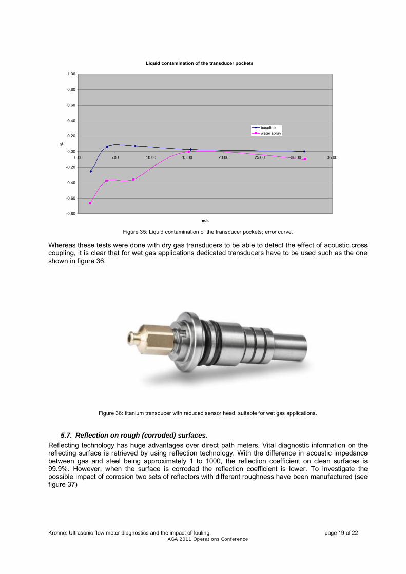
Figure 35: Liquid contamination of the transducer pockets; error curve.

Whereas these tests were done with dry gas transducers to be able to detect the effect of acoustic cross coupling, it is clear that for wet gas applications dedicated transducers have to be used such as the one shown in figure 36.

Figure 36: titanium transducer with reduced sensor head, suitable for wet gas applications.

5.7. Reflection on rough (corroded) surfaces.

Reflecting technology has huge advantages over direct path meters. Vital diagnostic information on the reflecting surface is retrieved by using reflection technology. With the difference in acoustic impedance between gas and steel being approximately 1 to 1000, the reflection coefficient on clean surfaces is 99.9%. However, when the surface is corroded the reflection coefficient is lower. To investigate the possible impact of corrosion two sets of reflectors with different roughness have been manufactured (see figure 37)

Liquid contamination of the transducer pockets

-0.80

-0.60

-0.40

-0.20

0.00

0.20

0.40

0.60

0.80

1.00

0.00 5.00 10.00 15.00 20.00 25.00 30.00 35.00

m/s

%

baselinewater spray


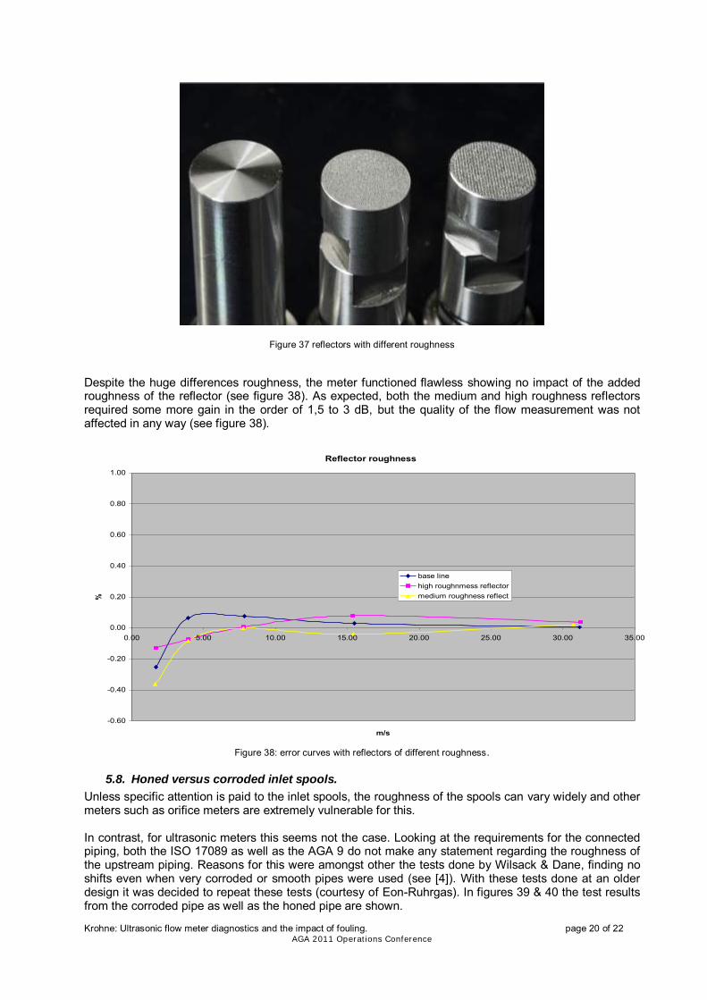
Figure 37 reflectors with different roughness Despite the huge differences roughness, the meter functioned flawless showing no impact of the added roughness of the reflector (see figure 38). As expected, both the medium and high roughness reflectors required some more gain in the order of 1,5 to 3 dB, but the quality of the flow measurement was not affected in any way (see figure 38).

Reflector roughness

-0.60

-0.40

-0.20

0.00

0.20

0.40

0.60

0.80

1.00

0.00 5.00 10.00 15.00 20.00 25.00 30.00 35.00

m/s

%

base linehigh roughnmess reflectormedium roughness reflect

Figure 38: error curves with reflectors of different roughness.

5.8. Honed versus corroded inlet spools.

Unless specific attention is paid to the inlet spools, the roughness of the spools can vary widely and other meters such as orifice meters are extremely vulnerable for this. In contrast, for ultrasonic meters this seems not the case. Looking at the requirements for the connected piping, both the ISO 17089 as well as the AGA 9 do not make any statement regarding the roughness of the upstream piping. Reasons for this were amongst other the tests done by Wilsack & Dane, finding no shifts even when very corroded or smooth pipes were used (see [4]). With these tests done at an older design it was decided to repeat these tests (courtesy of Eon-Ruhrgas). In figures 39 & 40 the test results from the corroded pipe as well as the honed pipe are shown.


Figure 39 corroded inlet spool Figure 40 Honed inlet spool Despite large differences in the upstream piping, the ALTOSONIC V12 calibration curves were not affected at all (see figure 41).

Honed versus corroded upstream pipe

-0.20

0.00

0.20

0.40

0.60

0.80

1.00

0.00 5.00 10.00 15.00 20.00 25.00 30.00 35.00

m/s

%

base line with corroded upstream pipebase line honed upstream pipe

Figure 41: calibration curves with honed and corroded inlet spools.


6. Conclusions

By using reflection technology, vital information on the conditions at the pipe wall is gathered and even small changes can be detected; long before it affects the accuracy of the custody transfer.

Exclusive to the patented design, even very small fractions of bottom fouling can be detected by

the vertical path. When changes are reported the developed first order correction functions give a reasonable

correction for both the bottom fouling as well as that of the evenly distributed fouling on the wall. For intermittent fouling the correction curve could not be fitted with the error curve and will be further investigated.

Reflective technology is in respect to accuracy and diagnostics far superior to direct chord

designs.

Although the SOS is a very powerful diagnostic parameter, it has to be used in combination with multiple other parameters to make a good evaluation of what is occurring inside the pipe. Other essential parameters: Signal strength Reflection coefficient Standard deviation on the flow velocity & SOS Signal to noise ratio’s Flow profile changes (suitable for large changes in the wall roughness). Trending and the build-up of an audit trail starting at the FAT, through calibration and

commissioning is essential.

The number of parameter and combinations of these are expanding and for the normal user too detailed. Expert software doing continuous analysis on these are going to be a necessity.

When using the Altosonic V12, if there is no change, the user can be confident that the original calibration curve is still valid.

7. Acknowledgments The authors thank Eon-Ruhrgas and especially Dr. Idriz Krajcin and Mr. Jörg Fasse for their contributions and excellent cooperation.

8. References [1] Diagnostics for reflective multipath ultrasonic meters. Jim Robertson, Pacific Gas and Electric Company, AGA Operations Conference, Dallas 2007 [2] A novel design of a 12 chords ultrasonic gas flow meter with extended diagnostic functions Jan G. Drenthen, Martin Kurth & Jeroen van Klooster. KROHNE New Technologies, AGA Operations Conference, Dallas 2007 [3] Reducing installation effects on ultrasonic flow meters. Jan G. Drenthen, Martin Kurth, Hilko den Hollander, Jeroen van Klooster & Marcel Vermeulen; Krohne. 7th International Fluid Flow Symposium, Anchorage 2009 [4] Wilsack, R., “Integrity of custody transfer measurement and ultrasonic technology.” CGA Measurement School 1996 [5] Witte, James “ Predicting Ultrasonic Meter Error in Dirty Service Conditions.” Ceesi Ultrasonic flow meter workshop Colorado Springs, 2010

ultrasonic flow meter diagnostics and the impact of . · pdf filekrohne: ultrasonic flow meter...

Documents