ultrasonic characterization of defects
TRANSCRIPT
SE0000134
SKI Report 99:25
Ultrasonic Characterization of Defects
Part 4. Study of Realistic Flaws in Welded Carbon Steel
Fredrik LingvallTadeusz Stepinski
February 1999
ISSN 1104-1374ISRNSKI-R--99/25-SE
3 1 - 1 4 .3
SKi

SKI Report 99:25
Ultrasonic Characterization of Defects
Part 4. Study of Realistic Flaws in Welded Carbon Steel
Fredrik LingvallTadeusz Stepinski
Uppsala University; Signals and SystemsBox 528, SE-751 20 Uppsala, Sweden
February 1999
SKI Project Number 97040
This report concerns a study which hasbeen conducted for the Swedish NuclearPower Inspectorate (SKI). The conclusionsand viewpoints presented in the reportare those of the authors and do notnecessarily coincide with those of the SKI.
Abstract
This report treats the ultrasonic measurements performed on the new V-welded carbon steelblocks and development of the algorithms for feature extraction, flaw position estimation, etc.Totally 36 different defects, divided into 8 types, were manufactured and implanted into theV-welds in the steel blocks. The flaw population can also be divided in two major groups: sharpflaws (various types of cracks and lack of fusion) and soft types of flaws (slag, porosity and overpenetration). A large amount of B- and D-scan measurements were performed on these flawsusing 6 different transducers. The evaluation of these measurements resulted in the conclusionthat the signal variation for the same type of defects is rather large compared to the variationfound in signals from artificial and simulated defects. The steel block measurements also revealedthat some of the defects were hard to distinguish, particularly if traditional features like fall/raisetimes, pulse duration and echo dynamics are used. To overcome this difficulty more powerfulfeature extraction methods were proposed, like the discrete wavelet transform and principalcomponent analysis. Another important subject that is treated in this report is the estimationof flaw positions from B-scans. The previously used, one dimensional method, appeared to besensitive to errors in the steel block measurements which, in some cases, resulted in poor flawposition estimates. Therefore, a two dimensional approach was proposed which should result inmore robust estimates due to the larger amount of data that is used for the estimation.
Sammanfattning
Denna rapport innehåller resultat från de mätningar som har gjorts på de nytillverkadestålblocken innehållande en V-svets med inplanterade "naturliga" defekter. Rapporten beskri-ver också de algoritmer som använts för estimering av position hos defekter, särdrags extraction(eng. feature extraction) mm. Totalt fanns det 36 olika defekter i stålblocken indelat i 8 olikatyper. Defekterna kan också delas in i två huvudgrupper: skarpa defekter (sprickor etc) ochmjuka (inklusioner, prorositet etc). Ett större antal B- och D-scan har samlats in med 6 olikasökare från dessa defekter. Utvärderingar av dessa mätningar visar att variationen hos signaleninom en defekttyp är stor jämfört med motsvarande mätningar gjorda för simulerade och artifi-ciella defekter. Det har även visat sig att det är svårt att skilja på vissa typer av defekter vilketbetyder att vi förmodligen har överlappande beslutsområden. Detta är speciellt tydligt om vianvänder klassiska metoder för särdrags-extraktion som stigtid, falltid, pulslängd och ekodyna-mik. På grund av detta föreslås användning av mera kraftfulla metoder för att extrahera särdragvilka behåller mera information om ultraljudssignalen än vad de klassiska metoderna gör. Tvåförslag till sådana metoder är den diskreta wavelet transformen och PCA (principal componentanalysis). Vidare behandlas också estimering av position hos defekter vilken är vital eftersompositionen hos en defekt används för den senare djupnormeringen av ultradjudssiganlen. Dethar visat sig att den tidigare använda (en dimensionella) metoden för att hitta defektpositionerej är tillräckligt robust för mätningar gjorda från de nya naturliga defekterna. Därför föreslåsen tvådimensionell metod för denna estimering vilket bör ge betydligt mera robusta estimâteftersom en större mängd data används vid estimeringen.

Contents
1 Introduction 1
2 Realistic Test Blocks 12.1 Description of the CS Test Blocks 1
3 Test Block Measurements 23.1 Transducers 2
3.2 Measurement Setup 3
3.3 Measurements 3
3.4 Results 3
3.4.1 Center Cracks 5
3.4.2 Sidewall Cracks 5
3.4.3 Lack of Fusion 8
3.4.4 Slag 9
3.4.5 Porosity 9
3.4.6 Root Crack 11
3.4.7 Lack of Penetration 11
3.4.8 Over Penetration 12
3.4.9 D-scans 12
4 Defect Characterization 144.1 Signal Features and Feature Extraction 14
4.1.1 Pre-processing 14
4.1.2 Finding Position of Defects 14
4.1.3 ROI Selection 14
4.1.4 Classical Features 15
4.1.5 Feature Extraction using the Discrete Wavelet Transform 16
4.1.6 Depth Normalization 17
4.2 Defect Classes 18
4.2.1 Crack-like Defects and Volumetric Defects 18
4.2.2 Defects at the Bottom of the Weld 21
4.3 Natural Contra Artificial Defects 22
5 Summary of Performed Work 22
6 Conclusions 24
Bibliography 26
A Comparison of the 2.25 MHz and the 3.5 MHz Transducers 27

B Carbon Steel Block Drawings 31
B.I PL4500 31
B.2 PL4501 32
B.3 PL4502 33
B.4 PL4503 34
l i
List of Figures
1 (a) Direct measurements (b) Indirect measurements (c) Backside measurements(d) D-scan 3
2 Indirect measurements from center cracks using the 45-degrees 3.5 MHz transducer(a) 3 mm crack, 10 mm from bottom surface (b) 6 mm crack, 26 mm from bottomsurface, tilted 2 degrees (c) 3 mm crack, 22 mm from bottom surface, 2 mm fromcenter of weld, tilted 3 degrees 6
3 Backside measurements from center cracks using the 60-degrees 3.5 MHz trans-ducer (a) 6 mm crack, 26 mm from bottom surface and tilted 2 degrees (b) 3 mmcrack, 22 mm from bottom surface, 2 mm from center of weld, tilted 3 degrees. . 6
4 Backside measurements from sidewall cracks using the 45-degrees 3.5 MHz trans-ducer (a) 3 mm crack, 24 mm from bottom surface (b) 7 mm crack, 29 mm frombottom surface (c) 7 mm crack, 17 mm from bottom surface 7
5 Backside measurements from sidewall cracks using the 60-degrees 3.5 MHz trans-ducer (a) 3 mm crack, 24 mm from bottom surface (b) 7 mm crack, 29 mm frombottom surface (c) 7 mm crack, 17 mm from bottom surface 7
6 Backside measurements from lack of fusion using the 45-degrees 3.5 MHz trans-ducer (a) 2.9 mm crack, 23.5 mm from bottom surface (b) 6.9 mm crack, 29.4mm from bottom surface (c) 6.9 mm crack, 17 mm from bottom surface 8
7 Backside measurements from lack of fusion using the 60-degrees 3.5 MHz trans-ducer (a) 2.9 mm crack, 23.5 mm from bottom surface (b) 6.9 mm crack, 29.4mm from bottom surface (c) 6.9 mm crack, 17 mm from bottom surface 8
8 Backside measurements from slag using the 45-degrees 3.5 MHz transducer (a) 3mm slag, 25 mm from bottom surface (b) 5 mm slag, 26 mm from bottom surface. 9
9 Backside measurements from slag using the 60-degrees 3.5 MHz transducer (a) 3mm slag, 25 mm from bottom surface (b) 5 mm slag, 26 mm from bottom surface. 9
10 Backside measurements from porosity using the 45-degrees 3.5 MHz transducer(a) 6 mm 'porosity, 22 mm from bottom surface (b) 8 mm porosity, 15 mm frombottom surface (c) 9 mm porosity, 26 mm from bottom surface 10
11 Backside measurements from porosity using the 60-degrees 3.5 MHz transducer(a) 6 mm porosity, 22 mm from bottom surface (b) 8 mm porosity, 15 mm frombottom surface (c) 9 mm porosity, 26 mm from bottom surface 10
12 Direct measurements from root cracks using the 60-degrees 3.5 MHz transducer(a) 3 mm crack, tilted 3 degrees (b) 3.4 mm crack, tilted 17 degrees (c) 7 mmcrack, tilted 27 degrees 11
13 Direct measurements from root cracks using the 60-degrees 3.5 MHz transducer(a) 3 mm crack, tilted 3 degrees (b) 3.4 mm crack, tilted 17 degrees (c) 7 mmcrack, tilted 27 degrees 11
14 Direct measurements from lock of penetration using the 60-degrees 3.5 MHz trans-ducer (a) 2 mm lack of penetration (b) 2.5 mm lack of penetration 12
15 Direct measurements from lack of penetration using the 70-degrees 3.5 MHz trans-ducer (a) 2 mm lack of penetration (b) 2.5 mm lack of penetration 12
16 Direct measurements from over penetration using the 60-degrees 3.5 MHz trans-ducer (a) 3 mm over penetration (b) 4-5 mm over penetration (c) 5 mm overpenetration 13
17 D-scans (a) 3 mm root crack (b) 5 mm over penetration 13
in

18 Echo-dynamics from (a) a sidewall crack and (b) a slag inclusion 15
19 The f o u r t i m e s used f o r calculating r i s e t i m e , p u l s e d u r a t i o n and fall t i m e . . . . 1 5
2 0 Envelope of A-scans from three different flaws (a) Slag inclusion (b) Over pene-tration (c) Center crack 16
21 The first 16 basis functions of the Coiflet 2 mother wavelet 17
22 (a) The echo-dynamics from a slag inclusion, (b) The first 16 wavelet coefficientsfrom the same A-scans as on (a) 17
23 Probe p o s i t i o n s seen f r o m a defect i n a g i v e n i n t e r v a l of o b s e r v a t i o n a n g l e . . . . 1 8
2 4 Envelope of A-scans from crack-like defects, (a)-(c) Center cracks (d)-(e) Side-wall cracks (f) Lack of fusion 19
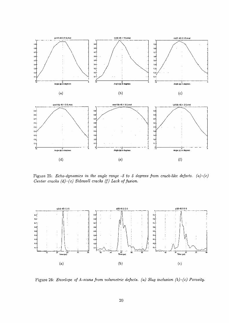
25 Echo-dynamics in the angle range -5 to 5 degrees from crack-like defects, (a)-(c)Center cracks (d)-(e) Sidewall cracks (f) Lack of fusion 20
26 Envelope of A-scans from volumetric defects, (a) Slag inclusion (b)-(c) Porosity. 20
27 Echo-dynamics in the angle range -5 to 5 degrees from volumetric defects, (a)Slag inclusion (b)-(c) Porosity 21
28 Envelope of A-scans from Defects in the bottom of the weld, (a) Over penetration(b) lack of penetration and (c) root crack 21
29 Four artificial cracks (notches) in the Bl aluminum block 22
30 One A-scan from a crack (notch) in aluminum block Bl. (a) A-scan and (b)Envelope of the same A-scan 23
31 A fictitious two feature example 24
32 Center crack #19 with the 45 degree wedge (A-scans at 52 mm from the weld). . 27
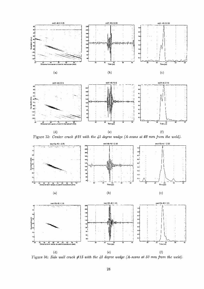
33 Center crack #21 with the 45 degree wedge (A-scans at 62 mm from the weld). . 28
34 Side wall crack #15 with the 45 degree wedge (A-scans at 50 mm from the weld). 28
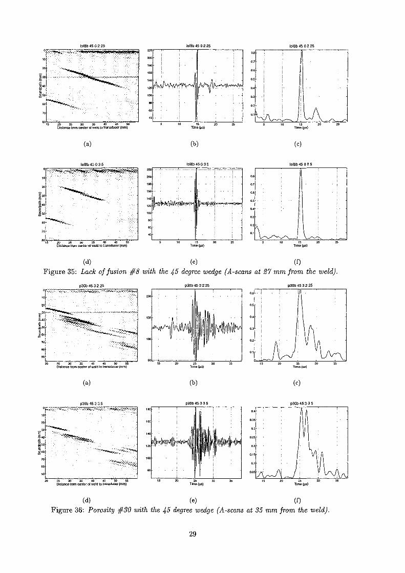
35 Lack of fusion #8 with the 45 degree wedge (A-scans at 21 mm from the weld). . 29
36 P o r o s i t y # 3 0 w i t h the 4 5 degree wedge ( A - s c a n s a t 3 5 m m from t h e weld). . . . 2 9
3 7 Side wall crack #18 with the 70 degree wedge (A-scans at 33 mm from the weld). 30
List of Tables
1 Flaw list 2
2 Transducer list 2
3 B-scan measurements made on the Steel-block welds with both 2.25 MHz and 3.5MHz Transducers 4
4 B-scan measurements made on the aluminum blocks with artificial defects. Themeasurements were made with the 2.25 MHz and 3.5 MHz transducers 5
IV
1 Introduction
This report treats the ultrasonic measurements performed on the new V-welded carbon steelblocks and development of algorithms for feature extraction, flaw position estimation, etc. Thesoftware used below is partly based on the software used for immersion testing of simulatedand artificial defects from the previous project Ultrasonic Characterization of Defects [1, 2, 3].However, there has been a substantial rewriting of the algorithms, and new algorithms have alsobeen added to fit the new contact measurements of the V-welded steel blocks. A substantial efforthas also been put in complementary manual inspection related to interpreting the ultrasonicdata obtained from the scanner. Section 2 describes the manufacturing of the new carbon steelblocks and the "natural" flaws that are implanted in them. The main part of the text, Section 3,describes the B-scan (and D-scan) measurements that have been performed and discusses thefeatures found in the measurements. In Section 4 the algorithms for: position estimation, regionof interest selection, feature extraction, and depth normalization are presented. This sectionalso contains a discussion of the different defect classes proposed and a comparison of signalfeatures between different flaw types. At the end of the section there is also a comparison ofartificial flaws contra natural flaws. Finally, Section 5 gives a summary of performed work andSection 6 gives the conclusions.
2 Realistic Test Blocks
The first step of the project Ultrasonic Defect Characterization includes designing and manufac-turing test blocks made of carbon steel (CS) containing realistic flaws in the weld. The originalplanning concerned 12 welded blocks, each with 3 flaws in the V-weld. After the discussion withthe manufacturer (Sonaspection International Ltd.) the number of blocks has been reducedto four, mainly due to the substantial difference in production cost. Other important factorsupporting this change was related to logistics in our laboratory which is not well prepared forhandling heavy steel loads. It should be noted however, that despite the reduced number ofblocks, the number of flaws has remained the same as planned, i.e. total 36 flaws of differenttypes. Thus this change does not influence the extend of the experimental work. We decidedto split block manufacturing in two steps, first to get CS blocks and then, after acquiring andprocessing ultrasonic data from the flaws, to manufacture similar blocks made of stainless steel(SS). The main reason for that is the need of practical experience before deciding what types offlaws should be manufactured in the SS blocks. However, the manufacturing of the SS blockshas been postponed for reasons which will be explained later in this report.
2.1 Description of the CS Test Blocks
Four blocks, each with 9 various flaws, were designed in collaboration with, and manufacturedby Sonaspection International Ltd. All blocks have dimensions 42 mm x 400 mm x 600 mmand consist of two carbon steel plates, welded together (V-weld). The defect types and sizesmanufactured in the blocks are summarized in Table 1. From Table 1 can be seen that ourflaw population consists of 24 sharp flaws (various types of cracks and lack of fusion) and 12soft type flaws (slag, porosity and over penetration). Closer analysis shows that we have threedifferent types of cracks characterized by various sizes, angles and locations. The cracks weremanufactured by mechanical fatigue and were implanted by semi-direct insertion (created beforethe welding process or at a pre-determined stage during welding). We have also natural sharpflaws in the form of lack of side wall fusion. This gives an idea of spread in the sharp flawclass which should also result in the variation of their ultrasonic signatures. On the other handsoft defects by their nature should result in similar ultrasonic responses, independent of their

Flaw TypeRoot CrackRoot CrackLack of Side Wall FusionLack of Side Wall FusionSide wall crackSide wall crackCenter line crackCenter line crackSlagPorosityOver PenetrationLack of Penetration
Size in mm36373736
3-66-103-52-25
No of flaws333333333333
AbbreviationsRCRC
LOFLOF
swcswcccccsp
OPLOP
Table 1: Flaw list.
location and size.
Sonaspection delivered detailed drawings of the blocks, as built flaw details and photographsof flaw signatures for each crack. Copies of Sonaspection block drawings are in Appendix B. Acopy of the Sonaspection report was delivered to SKi. The test blocks have been subjected tocareful ultrasonic inspected in our lab and all the defects were localized according to the reportsfrom Sonaspection.
3 Test Block Measurements
This section describes the used transducers, the measurement setup, and the measurementsperformed.
3.1 Transducers
The contact UT inspection of the blocks has been performed using mechanized scanner and adigital ultrasonic system based on Saphir PC board. B-scans for each flaw were acquired and aflaw data base has been created.
Two miniature screw-in transducers from Panametrics, with center frequencies 2.25 MHz(type V539-SM) and 3.5 MHz (type A545S-SM) were used in the (shear wave) contact inspection:Both transducers had nominal element size 0.5" (13 mm) and were assembled by screwing
/o [MHz]2.252.252.253.53.53.5
B [MHz] (-6dB)89%89%89%58%58%58%
Angle [Degrees]456070456070
ProducerPanametricsPanametricsPanametricsPanametricsPanametricsPanametrics
Table 2: Transducer list.
directly into miniature angle beam wedges type ABWM-5T also from Panametrics. Six different
angle beam transducer configurations, listed in the Table 2 above, were created in this way.Advantage of this solution is quite obvious, by using the same active element we have obtainedangle transducers with very similar characteristics. Since ultrasonic response of a particularflaw is determined both by the flaw type and by the transducer characteristics it is essential fordefect characterization to keep transducer characteristic as constant as possible.
3.2 Measurement Setup
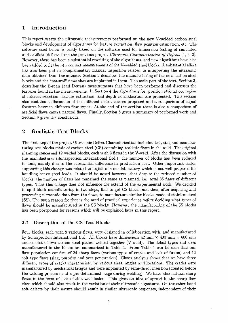
Four different scanning methods were used. The aim was to make direct measurements from thetop side of the steel blocks shown in Figure la. However, for smaller angles direct measurementswere obstacled by the upper surface of the V-weld. In such cases indirect measurements ormeasurements from the backside were performed instead, which is shown in Figure lb andc. Another reason for making indirect (or backside) measurements was low amplitude of the
f" 1
A /\/(a)
w(b)
.--
k 1\l
(c) (d)
Wclii
Figure 1: (a) Direct measurements (b) Indirect measurements (c) Backside measurements (d)D-scan.
reflection obtained in the direct measurement due to the angle between the transducer mainbeam and certain flaws, like sidewall cracks.
The fourth scanning method is shown in Figure Id, which is so-called D-scans. That is,the probe is moved along the weld side-wise. D-scans are interesting because they reveal howthe defect response varies along the defect. It is also interesting to see the response from theweld itself, both with and without a defect present. Typically the shape of the weld variessubstantially spatially and D-scan shows this variation rather clearly.
3.3 Measurements
The performed measurements are displayed in Table 3 and Table 4. The measurements consistof B- and D-scan data matrices and the total number of measurements are 2x133. The mainpart of data comes from the welded steel blocks described above, but new measurements havealso been performed, for comparison, on the two old aluminum blocks with artificial defectsused in the previous project [3]. In addition to these measurements all flaws have also beeninvestigated manually.
The artificial flaws in Table 4 named SBH are side-drilled holes, and the ones named S arecracks (notches).1
3.4 Results
In this section a number of B-scans from each defect type are shown for illustration. They areselected so that both common features and feature variations are represented for each defect type.Note also, that some of the images contain echos from non-defect parts of the weld, like the top
'For a more detailed description of the aluminum blocks see [3].

Defect
R C lRC2RC3RC4RC5RC6L0F7L0F8L0F9LOF 10LOF 11LOF 12SWC 13SWC 14SWC 15SWC 16SWC 17SWC 18CC19CC 20CC21CC 22CC23CC 24S25S26S 27P 28P 29P 30OP 31OP 32OP 33LOP 34LOP 35LOP 36
Direct45 60
••••••
••••••
70
••••••
•
•
••
Indirect45
•••••••
••••••
60
•••••••
••
70Backside
45
••
••
•••••
•
••••
60
••
••
••••••
••
•
•••
••
70
•
•
•••
•
D-scan45
•
•
•
•
60••••••••
•
••••
••
•
•
••
••
••••••
70
•
•
•
Table 3: B-scan measurements made on the Steel-block welds with both 2.25 MHz and 3.5 MHzTransducers.

DefectS4-7S7-4SBH1SBH2SBH3SIS2S3S4S5S6
45•••••••••••
60
••••••
BlockBlBlBlBlBlB2B2B2B2B2B2
Table 4: B-scan measurements made on the aluminum blocks with artificial defects. The mea-surements were made with the 2.25 MHz and 3.5 MHz transducers.
or bottom surface of the weld or the steel-weld junction. These echos are explained (if possible)when they are encountered. In the figure titles the name of the data files are given. An exampleis p28b 1 3 5, where p28 means porosity flaw 28, b means backside measurements, 1 indicatesthat the flaw is located in test block PL4501, and 3 5 is the used transducer frequency (3.5MHz). The B-scans presented in the following subsections are from measurements with the 3.5Mhz transducer. The reason for showing the 3.5 Mhz transducer only is that the measurementsis performed on carbon steel blocks with very little material grain noise. This implies that the2.25 MHz and the 3.5 MHz transducers should give similar results with the exception that the3.5 MHz transducer has a higher center frequency and thus shorter wavelength and thereforehigher resolution (both transducers has approximately the same bandwidth). There is, however,a comparison of the two transducers in Appendix A.
3.4.1 Center Cracks
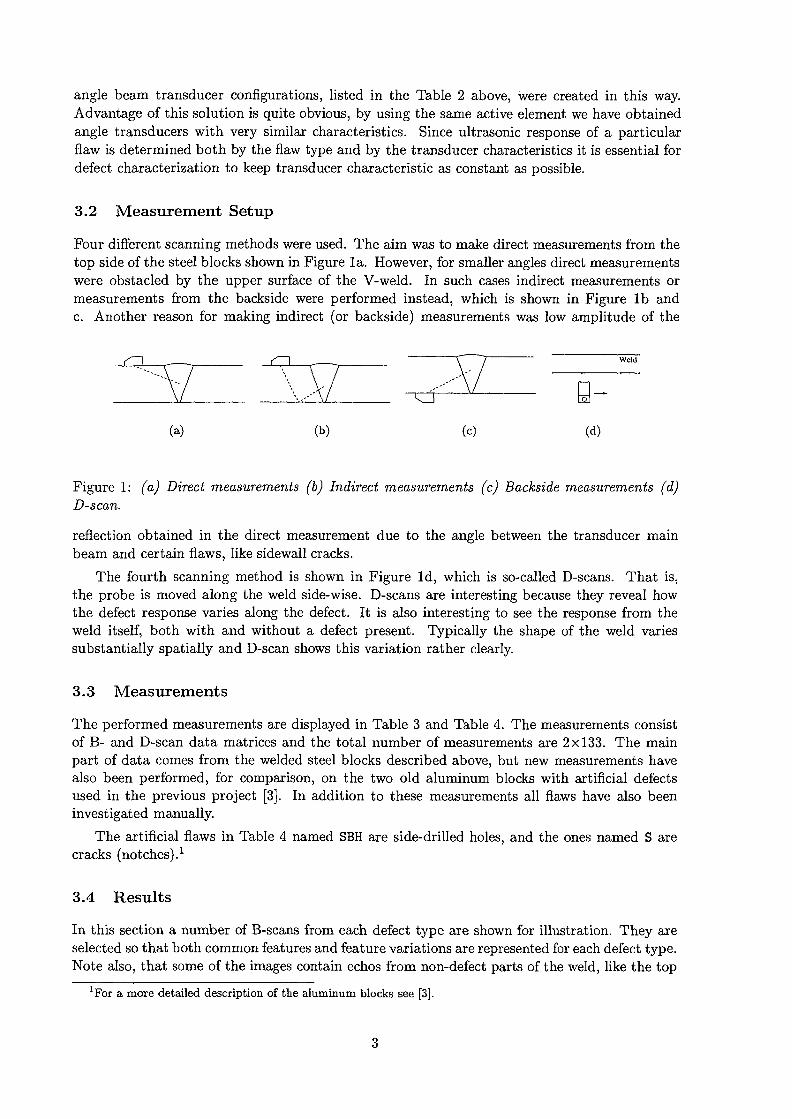
The center cracks found in the steel test blocks can be either straight or slightly tilted. Figure 2shows indirect measurements using the 45-degrees 3.5 MHz transducer. All echos around 60 mmstem from direct reflections from the bottom surface of the weld and all echos around 120 mmstem from indirect reflections from the top surface of the weld. One can see that there are tworather strong peaks (too strong to be diffraction echos) in all three B-scans. We can not findan unambiguous explanation for the presence of the second echos, but we believe that it mustdepend on the structure of the cracks implanted into the weld. These two peaks do not alwaysoccur in signals from center cracks, if we for example scan the defect in Figure 2a from the otherside of the weld, we get only a single peak. This effect is also less pronounced if a higher angleprobe is used. Figure 3 shows B-scans of the same defects obtained with a 60 degree transducer,and there is for example only one peak in Figure 3b (see Section 5 for a further discussion onthis topic).
3.4.2 Sidewall Cracks
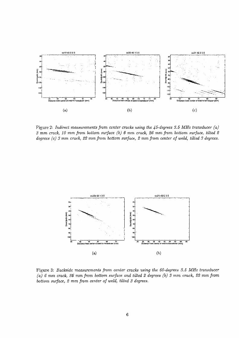
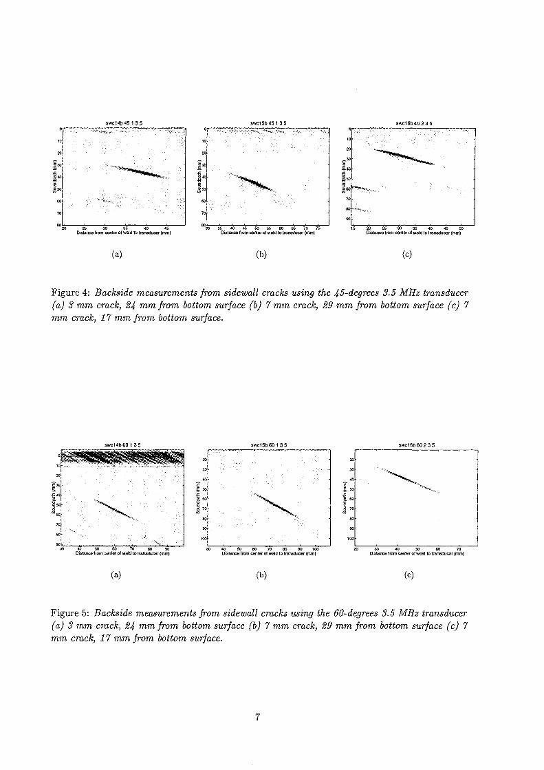
The sidewall cracks are located in the steel-weld junction and are therefore tilted with the sameangle as the weld (30 degrees). This makes it difficult to apply direct measurements and allmeasurements are therefore performed from the backside or indirect. Figure 4 and Figure 5show backside measurements performed with the 3.5 MHz 45- and 60-degrees transducers.All echos around 60 mm for the 45-degree transducer, and around 84 mm for the 60-degree
Distance Irom center of weld to transducer (mm)
(a)
Distance Irom center ot weld to transducer (mm) Distance Irom center d weld to transducer (mm)
(b) (c)
Figure 2: Indirect measurements from center cracks using the 45-degrees 3.5 MHz transducer (a)3 mm crack, 10 mm from bottom surface (b) 6 mm crack, 26 mm from bottom surface, tilted 2degrees (c) 3 mm crack, 22 mm from bottom surface, 2 mm from center of weld, tilted 3 degrees.
cc20b 60 1 3 5 cc21b 6 0 2 3 5
Distance from center ot weld to transducer (mm) Distance Irom center ot weld to transducer (mm)
(a) (b)
Figure 3: Backside measurements from center cracks using the 60-degrees 3.5 MHz transducer(a) 6 mm crack, 26 mm from bottom surface and tilted 2 degrees (b) 3 mm crack, 22 mm frombottom surface, 2 mm from center of weld, tilted 3 degrees.
SWC14D 45 1 3 5 swc15b45 1 3 5 swc16b45 2 3 5
Distance Irom center of weld to transducer (mm)30 35 40 45 50 55 GO 65 70 75
Distance from center of weld to transducer (mm)25 30
Distance Irom center ol weld 1o transducer (mm)
(a) (b) (c)
Figure 4: Backside measurements from sidewall cracks using the 45-degrees 3.5 MHz transducer(a) 3 mm crack, 24 mm from bottom surface (b) 7 mm crack, 29 mm from bottom surface (c) 7mm crack, 17 mm from bottom surface.
swc14b60135
40 50 60 70 80 90Distance from center ol weld to transducer (mm)
—
3pl
(a)
swc15b60135 swc16b602 3 5
Distance from center of weld to transducer (mm)
(b)
20 30 40 50 60 70Distance from center ol weld to transducer (mm)
(c)
Figure 5: Backside measurements from sidewall cracks using the 60-degrees 3.5 MHz transducer(a) 3 mm crack, 24 mm from bottom surface (b) 7 mm crack, 29 mm from bottom surface (c) 7mm crack, 17 mm from bottom surface.
transducer come from the top surface of the weld. No double echos, like for center cracks, arenoted for the sidewall cracks.
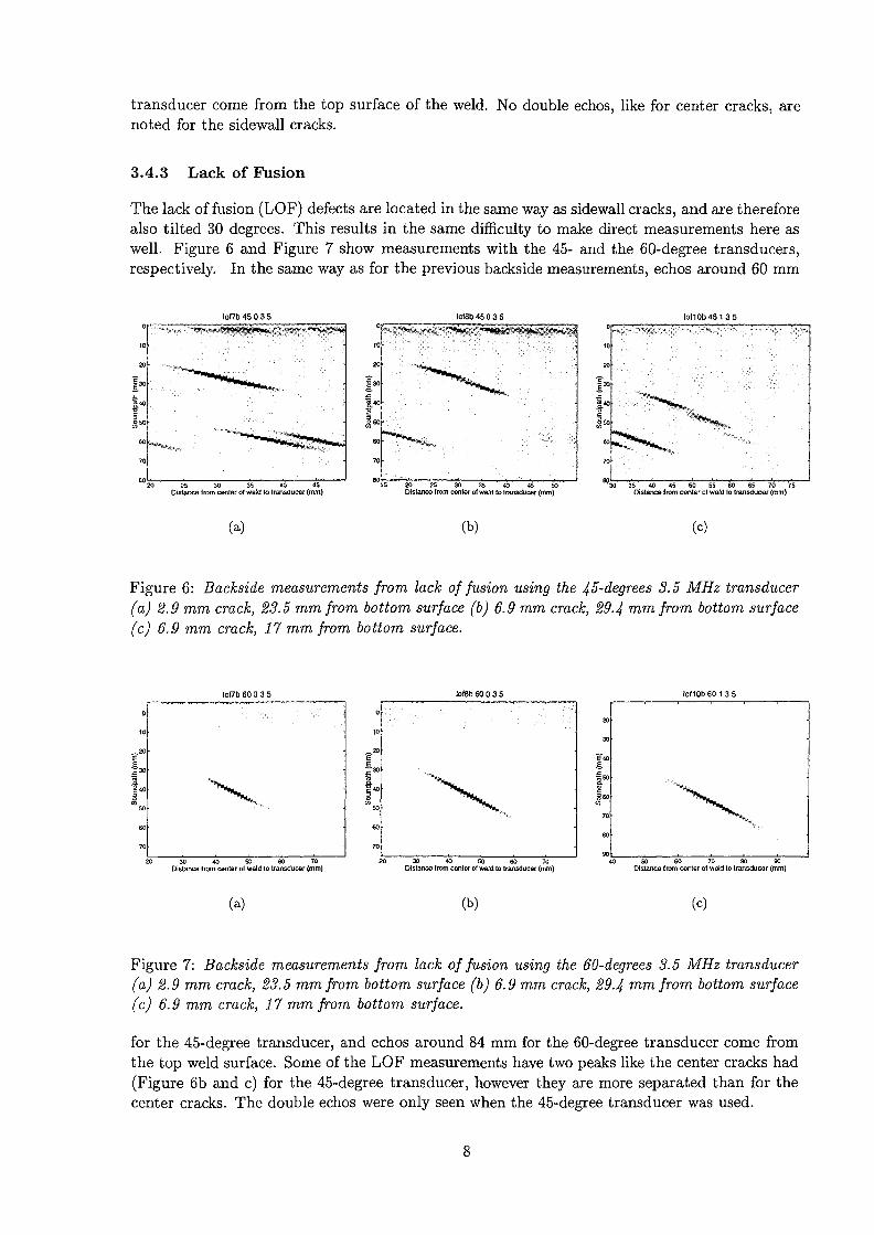
3.4.3 Lack of Fusion
The lack of fusion (LOF) defects are located in the same way as sidewall cracks, and are thereforealso tilted 30 degrees. This results in the same difficulty to make direct measurements here aswell. Figure 6 and Figure 7 show measurements with the 45- and the 60-degree transducers,respectively. In the same way as for the previous backside measurements, echos around 60 mm
Distance from center of weld 1o transducer (mm)
(a)
Iof8b450 35
15 20 25 30 35 _ _ _Distance from center of weld lo transducer (mm)
loll Ob 451 3 5
30 36 40 45 50 55 60 65 70 75Distance from center of weld to transducer (mm)
(b) (c)
Figure 6: Backside measurements from lack of fusion using the 45-degrees 3.5 MHz transducer(a) 2.9 mm crack, 23.5 mm from bottom surface (b) 6.9 mm crack, 29.4 Trim from bottom surface(c) 6.9 mm crack, 17 mm from bottom surface.
lofBb 60 0 3 5 loMOb 60 1 3 5
Distance Irom center of weld to transducer (mm) Distance from center ot weld to transducer (mm) Distance Irom center ol weld to transducer (mm)
(a) (b) (c)
Figure 7: Backside measurements from lack of fusion using the 60-degrees 3.5 MHz transducer(a) 2.9 mm crack, 23.5 mm from bottom surface (b) 6.9 mm crack, 29.4 mm from bottom surface(c) 6.9 mm crack, 17 mm from bottom surface.
for the 45-degree transducer, and echos around 84 mm for the 60-degree transducer come fromthe top weld surface. Some of the LOF measurements have two peaks like the center cracks had(Figure 6b and c) for the 45-degree transducer, however they are more separated than for thecenter cracks. The double echos were only seen when the 45-degree transducer was used.
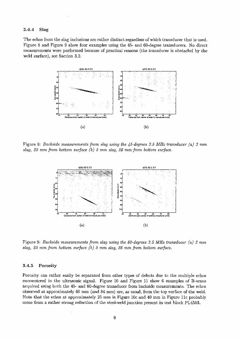
3.4.4 Slag
The echos from the slag inclusions are rather distinct regardless of which transducer that is used.Figure 8 and Figure 9 show four examples using the 45- and 60-degree transducers. No directmeasurements were performed because of practical reasons (the transducer is obstacled by theweld surface), see Section 3.2.
S27b 45 2 3 5
20 2SDis4ance from center ol weld to transducer (mm) Distance from center of weld lo transducer (mm)
(a) (b)
Figure 8: Backside measurements from slag using the 45-degrees 3.5 MHz transducer (a) 3 mmslag, 25 mm from bottom surface (b) 5 mm slag, 26 mm from bottom surface.
S25D600 3 5
Distance f ran center o) wold lo transducer (mm)50 60 70
Distance from center ol weld to transducer (mm)
(a) (b)
Figure 9: Backside measurements from slag using the 60-degrees 3.5 MHz transducer (a) 3 mmslag, 25 mm from bottom surface (b) 5 mm slag, 26 mm from bottom surface.
3.4.5 Porosity
Porosity can rather easily be separated from other types of defects due to the multiple echosencountered in the ultrasonic signal. Figure 10 and Figure 11 show 6 examples of B-scansacquired using both the 45- and 60-degree transducer from backside measurements. The echosobserved at approximately 60 mm (and 84 mm) are, as usual, from the top surface of the weld.Note that the echos at approximately 25 mm in Figure 10c and 40 mm in Figure 1 lc probablycome from a rather strong reflection of the steel-weld junction present in test block PL4503.

0
10
20
j»c
••a
80
p28b 45 0 3 5
•
p29b451 35 p30b 45 3 3 5
Distance Irom canter of wefd to transducer (mm)
(a)
2 2 »Distance from center of weld to transducer (mm) Distance from center ot weld to transducer (mm)
(b) (c)
Figure 10: Backside measurements from porosity using the 45-degrees 3.5 MHz transducer (a) 6mm porosity, 22 mm from bottom surface (b) 8 mm porosity, 15 mm from bottom surface (c) 9mm porosity, 26 mm from bottom surface.
p28b 60 0 3 5
30 35 40 45 SO 55 60 65 70Distance Irom center ot weld to transducer (mm)
p29b 60 1 3 5 p30b 60 3 3 5
20 25 30' 35 40 45 50 55 60 65Distance Irom center of weld to transducer (mm)
(a) (b)
30 S5 40 45 50 55 60 65 70 7!Distance irom center ol weld to transducer (mm)
(c)
Figure 11: Backside measurements from porosity using the 60-degrees 3.5 MHz transducer (a) 6mm porosity, 22 mm from bottom surface (b) 8 mm porosity, 15 mm from bottom surface (c) 9mm porosity, 26 mm from bottom surface.
10
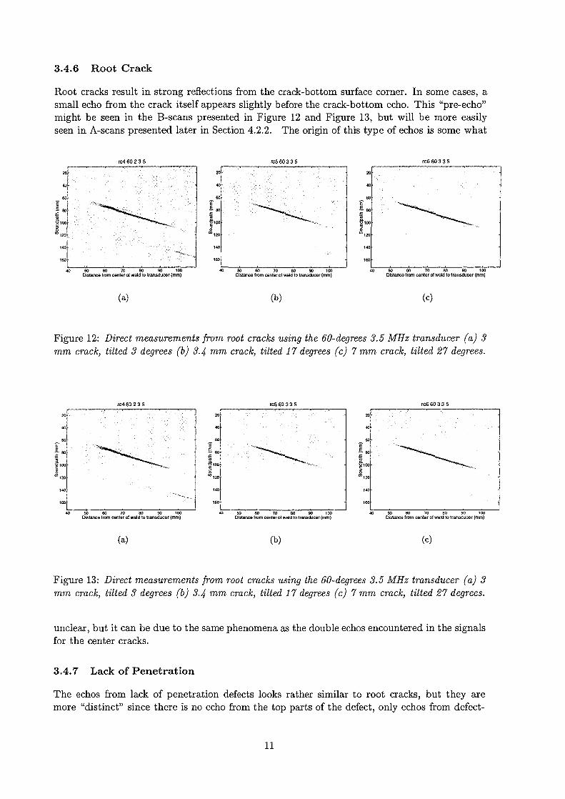
3.4.6 Root Crack
Root cracks result in strong reflections from the crack-bottom surface corner. In some cases, asmall echo from the crack itself appears slightly before the crack-bottom echo. This "pre-echo"might be seen in the B-scans presented in Figure 12 and Figure 13, but will be more easilyseen in A-scans presented later in Section 4.2.2. The origin of this type of echos is some what
rc5 60335
Distance 1rom center of weld to transducer (mm) Distance from center of weld to transducer (mm) Distance Irom center of weld to transducer (mm)
(a) (b) (c)
Figure 12: Direct measurements from root cracks using the 60-degrees 3.5 MHz transducer (a) 3mm crack, tilted 3 degrees (b) 3.4 rnm crack, tilted 17 degrees (c) 7 mm crack, tilted 27 degrees.
rc4 60235 rc5 60335
Distance from center of weld to transducer (mm) Distance from center of weld to transducer (mm) Distance from center 01 weld to transducer (mm)
(a) (b) (c)
Figure 13: Direct measurements from root cracks using the 60-degrees 3.5 MHz transducer (a) 3mm crack, tilted 3 degrees (b) 3.4 mm crack, tilted 17 degrees (c) 7 mm crack, tilted 27 degrees.
unclear, but it can be due to the same phenomena as the double echos encountered in the signalsfor the center cracks.
3.4.7 Lack of Penetration
The echos from lack of penetration defects looks rather similar to root cracks, but they aremore "distinct" since there is no echo from the top parts of the defect, only echos from defect-
11
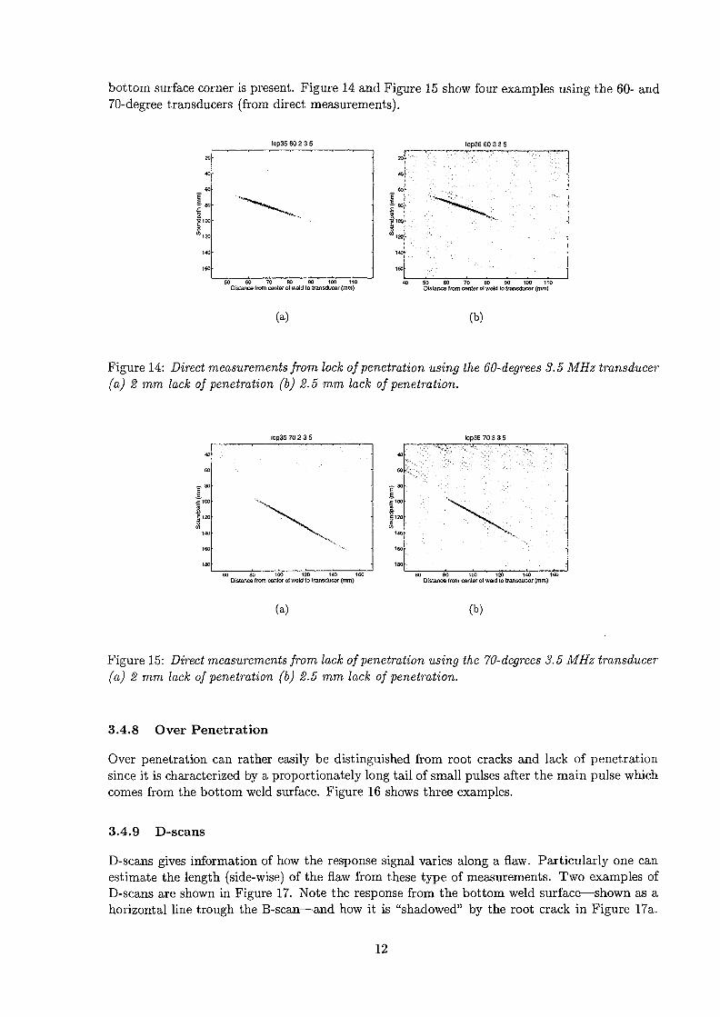
bottom surface corner is present. Figure 14 and Figure 15 show four examples using the 60- and70-degree transducers (from direct measurements).
Iop35 60 2 3 5
100 110Distance from center ol wald to transducer (mm)
Iop36 60 3 3 5
SO 60 70 80 90 100 110Distance from center of weld to transducer (mm)
(a) (b)
Figure 14: Direct measurements from lock of penetration using the 60-degrees 3.5 MHz transducer(a) 2 mm lack of penetration (b) 2.5 mm lack of penetration.
lop35 7O2 3 5
100 120 140Distance from center ol weld to transducer (mm)
(a)
1*0}-
Iop36 703 3 5
3 80 100 120 140 1Distance from center ol weld to transducer (mm)
(b)
Figure 15: Direct measurements from lack of penetration using the 70-degrees 3.5 MHz transducer(a) 2 mm lack of penetration (b) 2.5 mm lack of penetration.
3.4.8 Over Penetration
Over penetration can rather easily be distinguished from root cracks and lack of penetrationsince it is characterized by a proportionately long tail of small pulses after the main pulse whichcomes from the bottom weld surface. Figure 16 shows three examples.
3.4.9 D-scans
D-scans gives information of how the response signal varies along a flaw. Particularly one canestimate the length (side-wise) of the flaw from these type of measurements. Two examples ofD-scans are shown in Figure 17. Note the response from the bottom weld surface—shown as ahorizontal line trough the B-scan—and how it is "shadowed" by the root crack in Figure 17a.
12

op31 60 0 3 5 OP32 602 3 5
Distance from center of weld to transducer (nun)
(a)
Op33 60 3 3 5
Distance from center ol weld to transducer (mm)60 70 80
Distance from center ol wekt to transducer (mm)
(b) (c)
Figure 16: Direct measurements from over penetration using the 60-degrees 3.5 MHz transducer(a) 3 mm over penetration (b) 4-5 mm over penetration (c) 5 mm over penetration.
rc4 60235 op33 60335
A-scan (separation 1 mm) A-scan (separation 1 mm}
(a) (b)
Figure 17: D-scans (a) 3 mm root crack (b) 5 mm over penetration.
13

Note also the typical ringings after the weld surface response in Figure 17b that are characteristicfor the over penetration type of flaws.
4 Defect Characterization
4.1 Signal Features and Feature Extraction
4.1.1 Pre-processing
Currently, like in the previous study [1, 2, 3], we only look at the envelope of the collectedultrasonic B-scan data. The envelope is calculated by means of the Hilbert transform. Theresulting data is also smoothed with a low-pass filter to reduce the measurement noise presentin data.
4.1.2 Finding Position of Defects
The flaw position is used for both region of interest (ROI) selection and depth normalization, andit is therefore important to have accurate and robust position estimates. The current method tofind the flaw position is based on fitting an hyperbolic function to the flaw response in B-scandata, see [2]. This method is summarized below:
The curves formed by a point scatterer in a B-scan, obtained with the contact mea-suring setup in Figure la-c, are shaped as a part of an hyperbola given by theequation
r = \lxlansd + zflaw i1)
The position estimate (xtrQ,nsd,Zfiaw) is found by minimizing the summed squarederror ^ || r^ax ~ ?® ||2> « = 1,2,... , JV, for a selected number of A-scans, wherefmax is the position of the max amplitude of the envelope of the ith A-scan.
Another approach, which would be more robust is to fit a 2D-function (surface) to the flawresponse signal. Such a function would approximate the flaw response in a more unambiguousway than than the hyperbolic contour defined by Eq. (1). It would be more robust since manypoints of the 2D response would be used for its estimation. Or re-phrased, we use a flaw model,and adjust the parameters of this model so that a synthetic B-scan generated from this modelis as similar as possible to the original measured B-scan. One of the parameters of this modelwould then be the position of the flaw, which is exactly what we are searching for.
4.1.3 ROI Selection
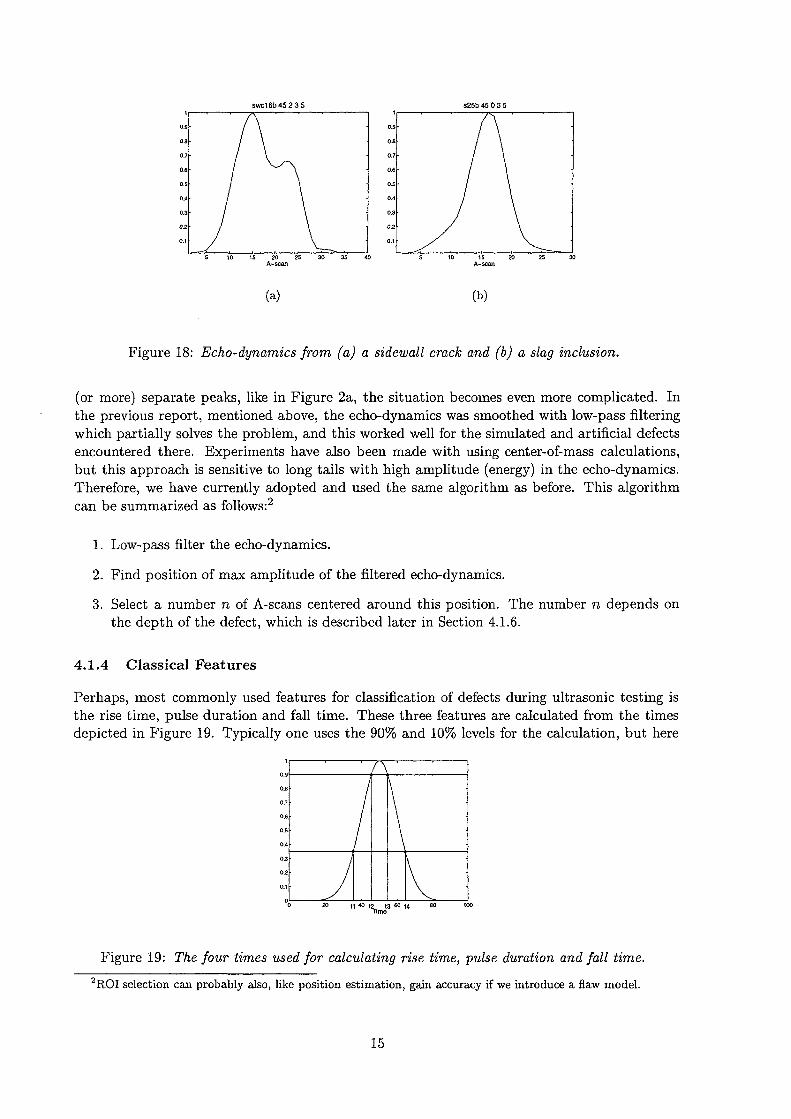
Selection of region of interest (ROI) is not a trivial task for the type of ultrasonic images obtainedfrom the "real" flaws encountered here. Ideally we would like to position an hyperbolic shapedanalyzing window around a flaw response signal in an B-scan image. The position of the windowshould be determined based only on the (exact) position of the flaw. The problem is that thedefect position is unknown and we have to estimate it, as mentioned in the previous section.However, this estimation is not accurate enough for the precise positioning required here. Inthe previous reports [2, 3] the echo-dynamics (max amplitude variation) of the flaw responsewas used for the positioning. Figure 18 shows two examples of echo-dynamics. As one can seethe echo-dynamics curves can be skew, have more than one peak, etc. If the B-scan has two
14
swo16b45 235
(a) (b)
Figure 18: Echo-dynamics from (a) a sidewall crack and (b) a slag inclusion.
(or more) separate peaks, like in Figure 2a, the situation becomes even more complicated. Inthe previous report, mentioned above, the echo-dynamics was smoothed with low-pass filteringwhich partially solves the problem, and this worked well for the simulated and artificial defectsencountered there. Experiments have also been made with using center-of-mass calculations,but this approach is sensitive to long tails with high amplitude (energy) in the echo-dynamics.Therefore, we have currently adopted and used the same algorithm as before. This algorithmcan be summarized as follows:2
1. Low-pass filter the echo-dynamics.
2. Find position of max amplitude of the filtered echo-dynamics.
3. Select a number n of A-scans centered around this position. The number n depends onthe depth of the defect, which is described later in Section 4.1.6.
4.1.4 Classical Features
Perhaps, most commonly used features for classification of defects during ultrasonic testing isthe rise time, pulse duration and fall time. These three features are calculated from the timesdepicted in Figure 19. Typically one uses the 90% and 10% levels for the calculation, but here
' A '
/
J\
Figure 19: The four times used for calculating rise time, pulse duration and fall time.2ROI selection can probably also, like position estimation, gain accuracy if we introduce a flaw model.
15
the same levels as in [3] (90% and 35%) are adopted to avoid problems with noise.
When 2D data are available (B-scans) one commonly uses the echo-dynamics (see previoussection) which gives a description of the amplitude variation between consecutive A-scans in aB-scan.
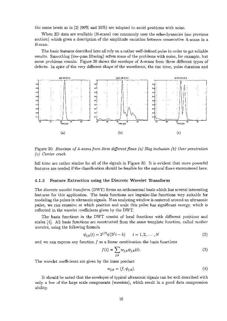
The basic features described here all rely on a rather well denned pulse in order to get reliableresults. Smoothing (low-pass filtering) solves some of the problems with noise, for example, butsome problems remain. Figure 20 shows the envelope of A-scans from three different types ofdefects. In spite of the very different shape of the waveforms, the rise time, pulse duration and
S25 45 0 3 5 op31 60 0 3 5 CC194503 5
40 45Time [psj
(a)
Time (ps)
(b)
Tims [us)
(c)
Figure 20: Envelope of A-scans from three different flaws (a) Slag inclusion (b) Over penetration(c) Center crack.
fall time are rather similar for all of the signals in Figure 20. It is evident that more powerfulfeatures are needed if the classification should be feasible for the natural flaws encountered here.
4.1.5 Feature Extraction using the Discrete Wavelet Transform
The discrete wavelet transform (DWT) forms an orthonormal basis which has several interestingfeatures for this application. The basis functions are impulse-like functions very suitable formodeling the pulses in ultrasonic signals. If an analyzing window is centered around an ultrasonicpulse, we can examine at which position and scale this pulse has significant energy, which isreflected in the wavelet coefficients given by the DWT.
The basis functions in the DWT consist of local functions with different positions andscales [4]. All basis functions are constructed from the same template function, called motherwavelet, using the following formula
^ h -k) t = l,2,...,N (2)
and we can express any function / as a linear combination the basis functions
The wavelet coefficients are given by the inner product
(3)
(4)
It should be noted that the envelopes of typical ultrasonic signals can be well described withonly a few of the large scale components (wavelets), which result in a good data compressionability.
16

There are several different types of pre-defined mother wavelets available in common softwarepackages, like the Wavelet toolbox for MATLAB. Figure 21 shows the first (largest scale) basisfunctions of the Coiflet 2 mother wavelet, which is a fairly smooth wavelet suitable for thisapplication. In Figure 22 the echo-dynamics and the first 16 DWT coefficients from the same
0.5* - 0
-0.!0.!
m o
-8JN 0
-0.50.5
O) 0-0.5
0.5^ 0
"§:!" 0
-0.50.5
£ 0-0.5
0.5CM 0
-8:1CD 0
"8:1CO 0
-0.50.5
-0.50.5
-81I 0
-0.50.5
-0.5-kA
Figure 21: The first 16 basis functions of the Coiflet 2 mother wavelet.
A-scans are displayed. One can clearly see how the echo-dynamics is reflected in the wavelet
s25b 45 0 2 25.mat - Echo dynamics S25b 45 0 2 25.mat - Wavelet coefficients
(a) (b)
Figure 22: (a) The echo-dynamics from a slag inclusion, (b) The first 16 wavelet coefficientsfrom the same A-scans as on (a).
coefficients.
4.1.6 Depth Normalization
In an ultrasonic B-scan, a defect located close to the transducer will be seen in a fewer A-scansthan a similar defect present further away from the probe, due to the lobe characteristics (cone-beam geometry) of the probe. If we look at the echo-dynamics from two flaws at different depths,the flaw closest to the transducer will have a narrower shape than the other flaw. A simple wayto normalize is to re-sample the echo-dynamics (or wavelet coefficients) in some angle interval.That is, the feature vector (or matrix) is re-sampled in an angular scale instead of the originallinear scale (Cartesian coordinate system). Figure 23 shows a defect and probe positions given
17
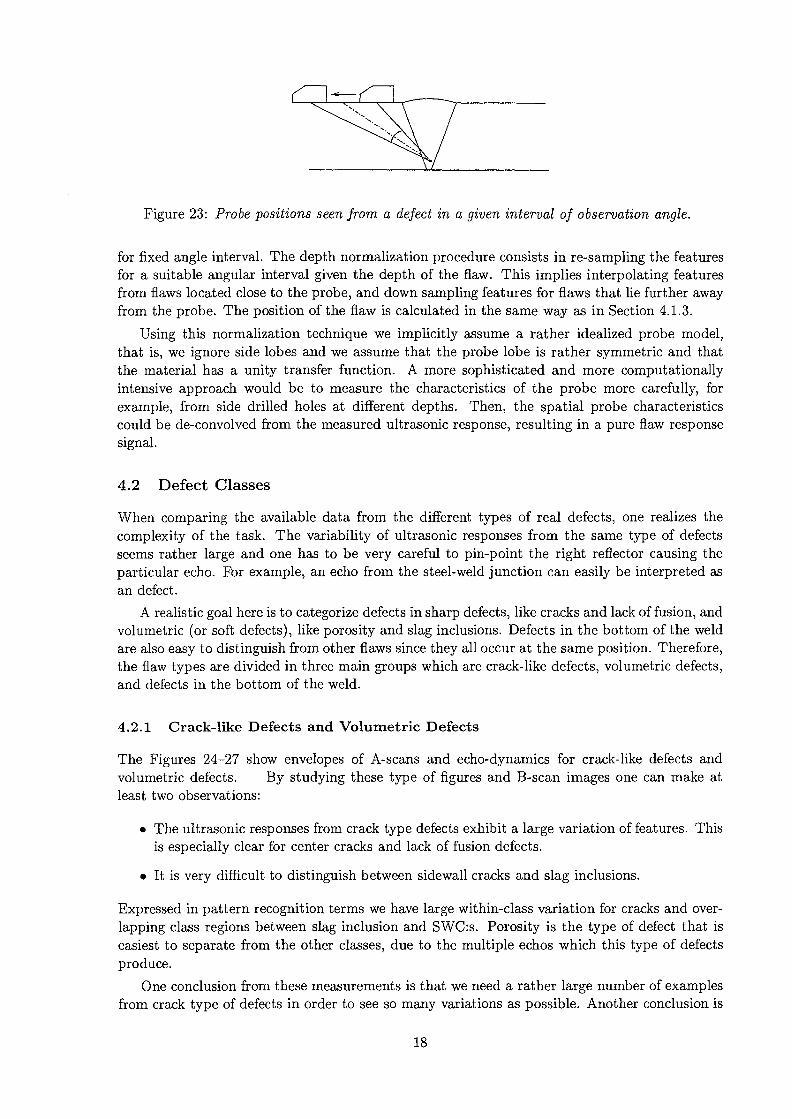
Figure 23: Probe positions seen from a defect in a given interval of observation angle.
for fixed angle interval. The depth normalization procedure consists in re-sampling the featuresfor a suitable angular interval given the depth of the flaw. This implies interpolating featuresfrom flaws located close to the probe, and down sampling features for flaws that lie further awayfrom the probe. The position of the flaw is calculated in the same way as in Section 4.1.3.
Using this normalization technique we implicitly assume a rather idealized probe model,that is, we ignore side lobes and we assume that the probe lobe is rather symmetric and thatthe material has a unity transfer function. A more sophisticated and more computationallyintensive approach would be to measure the characteristics of the probe more carefully, forexample, from side drilled holes at different depths. Then, the spatial probe characteristicscould be de-convolved from the measured ultrasonic response, resulting in a pure flaw responsesignal.
4.2 Defect Classes
When comparing the available data from the different types of real defects, one realizes thecomplexity of the task. The variability of ultrasonic responses from the same type of defectsseems rather large and one has to be very careful to pin-point the right reflector causing theparticular echo. For example, an echo from the steel-weld junction can easily be interpreted asan defect.
A realistic goal here is to categorize defects in sharp defects, like cracks and lack of fusion, andvolumetric (or soft defects), like porosity and slag inclusions. Defects in the bottom of the weldare also easy to distinguish from other flaws since they all occur at the same position. Therefore,the flaw types are divided in three main groups which are crack-like defects, volumetric defects,and defects in the bottom of the weld.
4.2.1 Crack-like Defects and Volumetric Defects
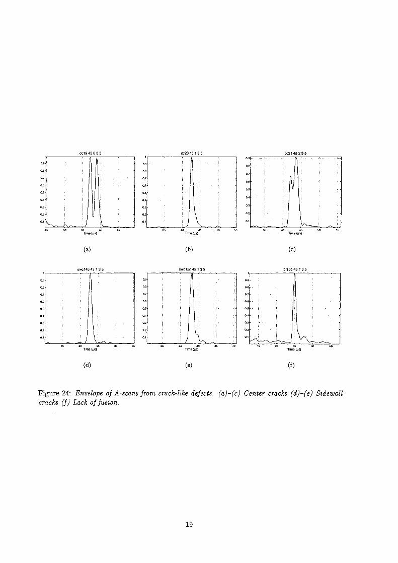
The Figures 24-27 show envelopes of A-scans and echo-dynamics for crack-like defects andvolumetric defects. By studying these type of figures and B-scan images one can make atleast two observations:
• The ultrasonic responses from crack type defects exhibit a large variation of features. Thisis especially clear for center cracks and lack of fusion defects.
• It is very difficult to distinguish between sidewall cracks and slag inclusions.
Expressed in pattern recognition terms we have large within-class variation for cracks and over-lapping class regions between slag inclusion and SWC:s. Porosity is the type of defect that iseasiest to separate from the other classes, due to the multiple echos which this type of defectsproduce.
One conclusion from these measurements is that we need a rather large number of examplesfrom crack type of defects in order to see so many variations as possible. Another conclusion is
18
CC20 45 1 3 5
! ' ' I
L : :Time (ps}
(a)
. 40 45 50Time Qis)
40 45Time (ps)
(b) (c)
swc14b 45 1 3 5 swo15t)45 135 Ioft0b45 135
(d) (e) (f)
Figure 24: Envelope of A-scans from crack-like defects, (a)-(c) Center cracks (d)-(e) Sidewallcracks (f) Lack of fusion.
19
cc19 45 0 3 5.mat
Angle ($) in degrees
(a)
cc20 45 1 3 5.mat
Angle («) In degrees
(b)
CC21 45 2 3 5.mat
Angle ($} in degrees
(c)
swc14b45 1 3 5.mat
Angle ($} in degrees
(d)
swc15b4S1 3 5.mat
Angle ($) in degrees
(e)
ton Ob 45 1 3 5.mat
Angle ($) in degrees
(f)
Figure 25: Echo-dynamics in the angle range -5 to 5 degrees from crack-like defects, (a)-(c)Center cracks (d)-(e) Sidewall cracks (f) Lack of fusion.
p28 45 0 3 5 p30 45 3 3 5
(a) (b) (c)
Figure 26: Envelope of A-scans from volumetric defects, (a) Slag inclusion (b)-(c) Porosity.
20

s25b45 0 3 5.mat
Angle ft>) in degrees
(a)
p28 45 0 3 5.mat
Angle ((,) In degrees
(b)
p30 45 3 3 5.mat
Angle {*) in degrees
(c)
Figure 27: Echo-dynamics in the angle range -5 to 5 degrees from volumetric defects, (a) Slaginclusion (b)-(c) Porosity.
that it seems to be very difficult to use the classical type of features as described in Section 4.1.4.That is, more sophisticated tools are needed and using the discrete wavelet transform is aninteresting option.
4.2.2 Defects at the Bottom of the Weld
The defects located at the bottom of the weld include three types of flaws: over penetration, lackof penetration, and root cracks. Figure 28 shows one example of each type. The within-class
op31 60 0 3 5 Iop34 60 1 3 5 rc4 60 2 3 5
A) I L i !•35 40 45 50
Time {(is)
(a) (b) (c)
Figure 28: Envelope of A-scans from Defects in the bottom of the weld, (a) Over penetration(b) lack of penetration and (c) root crack.
variation seems to be much smaller for the defects at the bottom of the weld than for the typescracks described in Section 4.2.1. The class separation between the three different flaw typesalso looks larger than the former case. Lack of penetration has a rather "clean" pulse shape,over penetration has typical ringings after the main pulse, and root cracks result often in a pulsewhich comes slightly before the main pulse, which is rather clearly seen in Figure 28c.
With classical features we might be able to separate the three flaw types. That is, if theringings of the over penetration and the "pre-pulse" of the root cracks are not separated too far
21

from the main pulse. A large separation between the ringings (or pre-pulse) and the main pulsewill result in that only the main pulse is used for feature extraction. In fact, the pre-pulse orringings might not even have a pulse amplitude that is higher than lower limit, which results ina total loss of these features.
However, if the DWT is used we preserve full information about the exact pulse shape andthere is no risk of loosing information of low amplitude pulses as long as they occur inside theanalyzing window.
4.3 Natural Contra Artificial Defects
As mentioned earlier B-scan data were also collected for the aluminum blocks with artificialdefects used in the previous reports. Figure 29 shows a B-scan from block Bl were four artificialcracks (notches) are located. The cracks have a depth of 2 mm, 4 mm, 4 mm and 8 mm (from
40
50
oCO
(LULU) H
Sou
ndpa
t!o
80
90
-
90
\
95 100
S4-7 45
\ \
105 110 115
-
•
V ----
120 125Distance from edge of block to transducer (mm)
Figure 29: Four artificial cracks (notches) in the Bl aluminum block.
left to right in the figure). One can clearly see the diffraction echos, whose location in the B-scanis in agreement with the size of the defects. Figure 30 shows one A-scan (and the envelope) fromthe same B-scan as in Figure 29. The pulse shape from the artificial defects are very "clean"compared to the ones from the steel blocks with real defects above. There are no double echosor irregular pulse shapes present in the signals from the artificial cracks in the aluminum data,as was the case for the real crack signals from the steel blocks. The defect characterization (i.e.classification) task becomes much simpler since the within-class variation is much lower thanfor real flaws. An implication of this is that the number of data needed "to span" the room ofpossible flaw signals is much lower for artificial defects than for the real defect counterpart. Thefeatures needed for classification are also simpler, echo-dynamics, rise time, pulse duration andfall time work well for artificial defects as shown in report [3], in contrary to the real flaw signalswere more sophisticated features are needed, as described above.
5 Summary of Performed Work
To begin with, all defects have thoroughly been investigated manually using hand hold probes.This was done in order to gain experience before a database of B- and D-scans were created.
22

S4-7 45
Time (us)
(a)
\ •
Time (us)
(b)
Figure 30: One A-scan from a crack (notch) in aluminum block Bl. (a) A-scan and (b) Envelopeof the same A-scan.
Based on experience from the manual inspection, B- and D-scan measurements where thenperformed using suitable transducers and transducer wedges. In addition to the carbon steelblock measurements additional measurements have also been performed on artificial defects inan aluminum block.
The ROI selection and feature extraction algorithms which previously were made for im-mersion measurements on aluminum blocks have been substantially re-written to 1) fit the newcarbon steel block measurements, and 2) to make it possible to incorporate new more powerfulfeature extraction techniques.
The measurements were then divided in three groups, volumetric (soft) defects, sharp defects(eg. cracks), and defects at the bottom of the weld. The measurements from these groups wherethen compared using: raw data, traditional features and the linear discrete wavelet transform.Additionally, the CS measurements were also compared to the data from the artificial defects inthe aluminum block and simulated data from the UT-Defect program [2, 5].
A substantial effort have been made on determining the origin of the double echos whichwere encountered in some of the measurements. It turned out to be very difficult to explain thephenomena based only on the measurements made using the techniques described in previoussections. One possible explanation of this is though, that the extra echos comes from structuresin the weld which is due to the manufacturing of the artificial defects. In order to make mea-surements with normal (0°) probes possible, one block was then send to an mechanical workshopwere the upper weld surface was machined off. Examining the measurements performed with anormal probe on, for example, center cracks resulted in strong reflections which normally shouldnot have been present. One could expect diffraction echos but such echos are several orders ofmagnitude lower than the echos encountered here. The most likely explanation is that the reflec-tion echo originates from implanted material (coupon) containing the crack. It is worth notingthat the coupon would not be detected by the radiographic examination due to unfavorableangle of the beams.
The final conclusion is that the double echos must be regarded as abnormal and hence notrepresentative as "real cracks". However, regarding the remaining defects, we still can see alarger variation in data than that for the artificial and simulated data.
Due, to the high signal variability no immersion measurements have been performed. Thereason for that is, obviously, that we need a number of enhancements to the signal processingtools before it is reasonable to acquire data from more difficult measurement situations, that is,
23

from immersion testing or from measurements of SS blocks.
6 Conclusions
During the evaluation of ultrasonic data acquired from the V-welded steel blocks it becameevident that the characterization task is much more complex than for the former simulated andartificial flaw signals. For example, in a V-weld there are other reflectors than flaws that resultin ultrasonic pulses, like the top and bottom weld surfaces and steel-weld junctions. The featurespace of possible flaw signals is also considerably larger for the real defects than for the artificialcounterpart. That is, the variation of the ultrasonic signals from one type (class) of defects ismuch larger for real than for artificial defects.
Our goal is to separate soft (or volumetric) defects from the sharper ones (crack-like), butif one studies the echo-dynamics and the pulse shapes (i.e. the envelope) of slag inclusions andside wall cracks it becomes apparent that they are very hard to separate. This implies thatwe might encounter overlapping feature regions—especially if we only use classical features likefall/raise times, pulse duration and echo dynamics. This is exemplified in Figure 31 where afictitious example characterized by only two features is shown. In this figure there are three
Figure 31: A fictitious two feature example.
classes present: one labeled A (with dashed boundary), and one B (with dotted boundary) andfinally class C (with dash-dotted boundary). There is also a number of examples from each classshown in the figure, where the x:es are from class A, the +:es from class B, and the o:es arefrom class C. As one can see class A and B are overlapping and they also have a low numberof examples which makes it very difficult to design a classifier with a proper decision boundary.Class C exemplifies the desired case with a sufficient number of examples and non-overlappingclass boundaries. To avoid this overlapping class boundary scenario, more powerful featureextraction algorithms are needed to achieve feasible classification performance.
High variation of the ultrasonic signals from the V-weld has also two further consequences:flaw position estimation can be poor (if the B-scan contains several peaks for example), and theamount of data needed to construct a reliable classifier is large.
Below, we list a number of conditions that must be fulfilled for a successful classifier
• Ensure that the measurements are good (informative) enough to distinguish between dif-ferent types of defects. This is vital, because we can of course not expect to be ableto distinguish between different defects if the information needed is not present in themeasurements.
• Representative features. The features that are fed to the classifier must preserve theinformation needed for successful classification.
24

• A sufficient number of examples. As a rule of thumb one needs at least ten times as many-examples as the parameters in the classifier, that is, to avoid that the classifier learnsthe training examples and performs poor on unseen examples. Moreover, we need enoughrepresentative examples to span the whole room of possible flaw signals for each defectclass. If the last condition is not fulfilled we get a classifier which is not able to classify alldefect signals properly.
The second condition is clearly not fulfilled with classical features and we must, therefore, utilizemore powerful methods. Examples of such methods are: wavelet analysis, principal componentanalysis (PCA) [6] and independent component analysis (ICA) [7]. The last two examplesare interesting since the basis functions used are completely determined from data. The firstcondition might not be fulfilled with a single B-scan measurements only. A common practice insuch situations when it is difficult to categorize a measurement is to combine measurements fromseveral transducers (with different angles, center frequencies etc.) and TOFD measurements.This technique is usually known as data fusion. The last condition is more cumbersome. Clearlywe do not have, and can not expect to have a sufficient number of examples to span the wholeroom of possible flaw signals, which is huge since we must account for different orientation, flawsize, crack roughness etc. Therefore, one could not expect to obtain a feasible classifier withthis low amount of data using a standard pattern recognition approach. Hence, we have toincorporate more knowledge, apart from the knowledge we obtained by looking at examples ofultrasonic data corresponding to available defects. Such knowledge can, for example, take formof expert knowledge of an experienced operator or the form of a flaw model. The simulated andthe artificial data (Section 4.3) showed a much lower signal variation than the real counterpart,and could therefore not be used to gain more training data. However, incorporating a model canstill supply us with some very valuable knowledge, like flaw position and perhaps flaw orientation.This knowledge would be very valuable for locating ROI, classification and normalization.3
To sum up the conclusions; we deal with a complex classification issue characterized by a highvariance in the defect classes and probably overlapping decision regions. Therefore, we have toimprove the signal processing algorithms, incorporate some type of expert knowledge, and obtainmore ultrasonic signals from various types of defects or introduce modeling. It is important tonote that we need compact data descriptions both to construct the classifier and for making theoptimization (model tuning) feasible, which otherwise would be very time consuming.
3The basic idea is to tune the model to generate data which resembles the real measurement as much aspossible.
25
References
[1] B. Eriksson and T. Stepinski. Ultrasonic charecterization of defects, part 1. literature review.Technical report, 1994. SKI Report 94:11.
[2] B. Eriksson and T. Stepinsk. Ultrasonic charecterization of defects, part 2. theoretical studies.Technical report, 1995. SKI Report 95:21.
[3] Bo Eriksson Tadeusz Stepinski and Bengt Vagnhammar. Ultrasonic charecterization of de-fects, part 3. experimantal varification. Technical report, 1996. SKI Report 96:75.
[4] Gilbert Strang and Truong Nguyen. Wavelets and Filter Bank. Wellesley - Cambridge Press,1996.
[5] A. Bostrom. Ut defect: A model of ultrasonic ndt of cracks. In 7th European Conference onNon-Destructive Testing, volume 3, pages 2414-2420, 1998.
[6] Keinosuke Fukanaga. Introduction to Statistical Pattern Recognition. Academic Press, secondedition, 1990.
[7] P. Comon. Independent component analysis, a new concept? Signal Processing, 36(3):287-314, April 1994.
26

A Comparison of the 2.25 MHz and the 3.5 MHz Transducers
This section show a comparison of the 2.25 MHz and the 3.5 MHz transducers for some of theflaws found in the V-welded steel blocks. Below a number of figures are shown where eachfigure corresponds to one particular flaw. All of the figures (Figure 32-37) has 6 sub-figures,labeled (a),(b), . . . ,(f), showing both B-scans, A-scans and the envelope of the A-scans. EachA-scan contains 1000 samples, which corresponds to an time interval of 25 //s, with the flawresponse centered in the middle of this interval. Note also that the envelope is smoothed. Thesub-figures (a)-(c) are for the 2.25 MHz transducer and the sub-figures (d)-(f) are for the 3.5MHz transducer.
During data acquisition the aim has been to scan the defects at the same position for boththe 2.25 MHz and the 3.5 MHz transducers. However, it is unavoidable to have some differencein probe position when changing transducer, which mostly shows in the response from the weldsurface which shape is rather irregular and thus can give a large change in the US responsesignal for small probe position variations.
CO19 45 0 2 25 CC1945 0 2 25 CC19 45 0 2 25
Distance from center of weld to transducer (mm) Time ftis)
(a) (b) (c)
CC19450 3 5
Distance Irom center o1 weld to transducer (mm)
i ;
Time (|JS)
(d) (e) (f)Figure 32: Center crack #19 with the 45 degree wedge (A-scans at 52 mm from the weld).
27
cc21 452225 CC2145 2 2 25 CC21 452225
f »? 80
Distance Irom center ot weld to transducer (mm) Time (fis)
(a) (b) (c)
CC21 45 2 3 5 cc2t 45 2 3 5
Distance Irom center ol weld to transducer (mm) Time Qis)
i35 40 45
Time (us)
(d) (e) (f)Figure 33: Center crack #21 with the 45 degree wedge (A-scans at 62 mm from the weld).
swo15b 45 1 2 25
J
swc15b45 1 2 25
30 36 " 40 45 SO 55 60 ~ 65 70 75Distance Irom center of weld to transducer (mm)
swc15b45 1 2 25
(a) (b) (c)
Swc15b45 1 3 5 swc15b45 1 3 5 swc15b45 1 3 5
30 35 40 45 SO 55 60 65 70 75Distance Irom center ol weld to transducer (mm)
25 30ime (us)
(d) (e) (f)Figure 34: Side wall crack #15 with the 45 degree wedge (A-scans at 50 mm from the weld).
28
Iof8b45 0 2 25 Iof8b45 0225 Iof.8b45 0 2 25
20 25 30 35 40 45 SODistance Irom center ol weld to transducer (mm)
(a)
Time (us)
(b) (c)
lofBb 45 0 3 5 lotBb 45 0 3 5 lOfSb 45 0 3 5
15 20 25 30 35 40 45 SODistance from center of weld to transducer (mm) Tim© (us) Time (\is)
(d) (e) (f)Figure 35: Lack of fusion #8 with the 45 degree wedge (A-scans at 27 mm from the weld).
p30b45 3 2 25 p30b45 3 2 25 p30b 45 3 2 25
25 3 0 3 5 «Distance trom center of weld to transducer (mm)
(a)
Time (us)
(b)
20 25Time (us)
(c)
p30b 45 3 3 5 p30b45 33 5
25 30 35 40 45 SO 55Distance from center of weld to transducer (mm)
0.4
0.35
0.3
0.25
0.2
0.1 S
0.1
0.05
p30b 45335
U
V-
^ ; H A
: •: i • r> • •
Time Qis)
(d) (e) (f)Figure 36: Porosity #30 with the 45 degree wedge (A-scans at 35 mm from the weld).
29

SWC18&70 3 2 25 s w d 8 b 7 0 3 2 25
25 30 35 40 45 50 55 60 65Distance Irom center of w&W 1o transducer (mm)
(a) (b)
0.9
0.8
0.7
0.6
0.5
0.4
0.3
0.2
0.1
SWC18D70 3 2 28
•
•
•
•
;
;
:
Time (ps>
(c)
swc18b70 3 3 5 swc18b703 3 5 swc18b70 3 3 5
H
20 25 30 35 40 45 SO 5£i 60 65Distance irom cenler ol weld to transducer (mm)
(d) (e) (f)
Figure 37: Side wall crack #18 with the 70 degree wedge (A-scans at 33 mm from the weld).
30
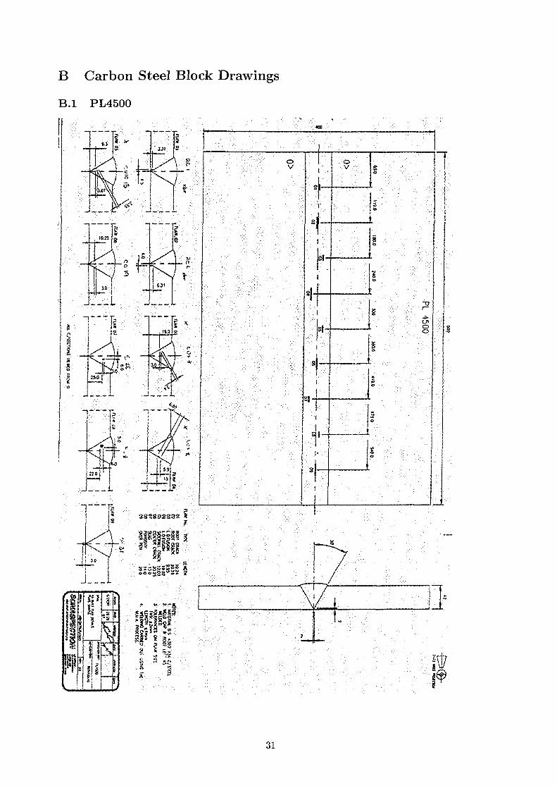
B Carbon Steel Block Drawings
B.I PL4500
M l
18.3 g
, <
* *
]
f I
i?
S828SS8S2
* * ¥£
400
• . • : ' • • ' / • • : . • . . . •
1 • • ' • • • . • . • .
• •' ..:::-;:v ' o. .. : . . ; - . ; • : • ; V
• • • . • • . •
• - ' . ' • • ' • • • • • • : . : . - . •
' ' • • • • " : • ' - . • : ' • • • [ • ' . ' •
' • . • . • • • . " . , . •
- • " • • ! • • • . • : • ' • ' • :
' • ; • • / • " • • • ' • • : • : • ' • ' • ' • ' ' •
. . • . . . • ; • . : • ' • •
• • ; . • : • . / • • . .
" • ' • • : - i . ' • • ' . • .
• ' . . • ' ' . " •
. : ' : . . . - . • ' . • • . - . . . . • ' " ! • • " .
' ' • • • • • • • • • : • . •
• : . . ' ' • •
. . . • : " •" .
• ' • ' . : . . •
• :
• - : • • • • . • . • ;
• . • • . • • • • • •
I •
i
f
L
:';:
r.
sf-
8
i'-.1-1i1I
•• : : © • • " • ' • •'
..v. "...
•
— -
v . . . : ' " • • . • . .
• • • • :
i • • •• • • • • .
o
'< • : ' ' ' : : • ' • : . ' : '
i
8 .::'r-::^:;• Z•' .-•• ':;• " . c ^ l
« > • • • • . •
• • •
* • ' " • • •
» • • - • • j
TT.
31
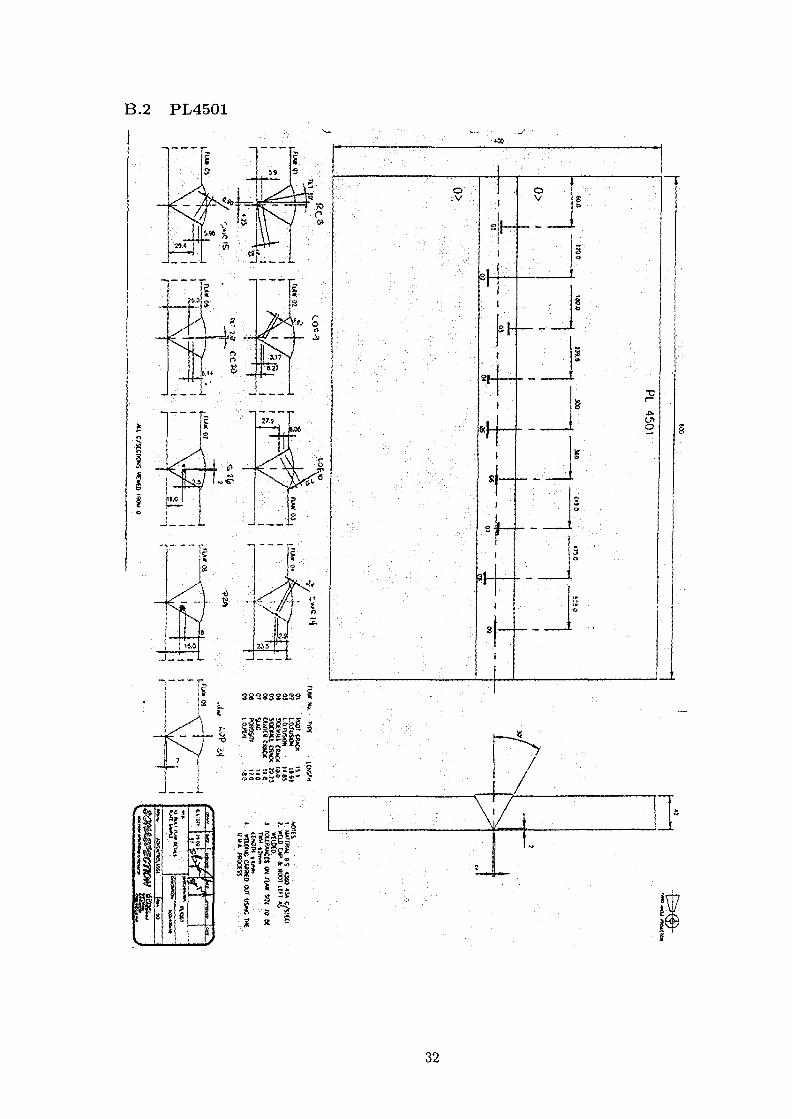
B.2 PL4501
32

B.3 PL4502
213
*00
1
o •V
oV
3
~T
o
33
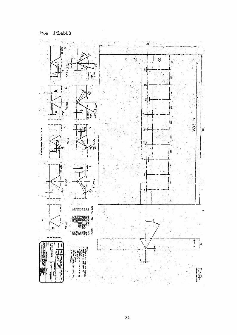
B.4 PL4503
• • : « » . .
• • . • . . -
' ' • • . . • : • • , . . . ; • • • . . . j • • • • : : : • • • • . • • • . . V • • . • . : • ' •
• ; " . " ' ' . , ' • ' © '
V
• : " . • • • • •
• • ; • • • ' • • •
I
- j
o l
1,
•
~1
2-f—
1
AI
f".I
1
1
oV
• . • • • ' . • ' •
1
— — _
8 ,. ..:.
* - . • .
o
•
w
s
—rU
J.
34

www.ski.se
STATENS KARNKRAFTINSPEKTION
Swedish Nuclear Power Inspectorate
POST/POSTAL ADDRESS SE-106 58 Stockholm
BESOK/OFFICE Klarabergsviadukten 90
TELEFON/TELEPHONE +46 (0)8 698 84 00TELEFAX +46 (0)8 661 90 86
E-POST/E-MAIL [email protected]
WEBBPLATS/WEB SITE WWW.ski.se