arX

iv:1

711.

0777

1v1

[cs

.IT

] 2

1 N

ov 2

017

1

Ultra-Reliable Low Latency Communication

(URLLC) using Interface DiversityJimmy J. Nielsen, Member, IEEE, Rongkuan Liu, and Petar Popovski, Fellow, IEEE

Abstract—An important ingredient of the future 5G systemswill be Ultra-Reliable Low-Latency Communication (URLLC). Away to offer URLLC without intervention in the baseband/PHYlayer design is to use interface diversity and integrate multiplecommunication interfaces, each interface based on a differenttechnology. In this work, we propose to use coding to seam-lessly distribute coded payload and redundancy data acrossmultiple available communication interfaces. We formulate anoptimization problem to find the payload allocation weights thatmaximize the reliability at specific target latency values. In orderto estimate the performance in terms of latency and reliabilityof such an integrated communication system, we propose ananalysis framework that combines traditional reliability modelswith technology-specific latency probability distributions. Ourmodel is capable to account for failure correlation amonginterfaces/technologies. By considering different scenarios, wefind that optimized strategies can in some cases significantlyoutperform strategies based on k-out-of-n erasure codes, wherethe latter do not account for the characteristics of the differentinterfaces. The model has been validated through simulation andis supported by experimental results.

Index Terms—Communication system reliability, diversitymethods, redundancy, codes, real-time systems.

I. INTRODUCTION

The upcoming 5G technology is designed for three main use

cases, namely enhanced Mobile Broadband (eMBB), massive

Machine-Type Communications (mMTC), and Ultra-Reliable

and Low Latency Communication (URLLC) [1]. URLLC may

be supported both through the 5G new air interface [2] or

through the integration of different existing communication

technologies [3] [4]. URLLC will enable the support of new

use cases under the umbrella of mission critical Machine-

type Communications (MTC), whose requirements exceed

the capabilities of current wireless technologies. Reliability

requirements in terms of packet delivery success rates may

be as high as 5-nines (1−10−5) to 9-nines (1−10−9), while

also the acceptable latency may be at the sub-second level or

even down to a few milliseconds [5]. There are proposals for

how to decrease the latency in future cellular systems, e.g., by

reducing the Transmission Time Interval (TTI) [6], [7], fast

uplink access [8], or by puncturing URLLC resources on top

of eMBB [2]. However, the benefits of such improvements

cannot be reaped until the features have been widely rolled

out. Furthermore, very high levels of reliability are difficult to

achieve with any single wireless communication technology,

Jimmy J. Nielsen and Petar Popovski are with the Department of ElectronicSystems, Aalborg University, 9220 Aalborg, Denmark, e-mail: jjn@es.aau.dk,petarp@es.aau.dk

Rongkuan Liu is with the Communication Research Center, Harbin Instituteof Technology, Harbin 150001, China, e-mail: liurongkuan@hit.edu.cn.

and is as such expected to be reachable through the integration

of multiple communication technologies [9].

The use of multiple communication technologies is concep-

tually very similar to many existing multipath protocols that

increase end-to-end reliability [10]. However, the strict latency

requirements of mission critical MTC, exclude protocols that

rely on retransmission. Instead we focus on interface diversity

which is in fact path diversity [11], where each path must

use a different communication interface. While there are many

multipath protocols [10], we have not identified any works that

allow to flexibly trade-off latency and reliability, as considered

in this paper. The closest examples of related work that

we have identified are the following. In [12], the authors

demonstrate the use of Software Defined Networking (SDN) to

distribute application packets across multiple available inter-

faces to increase application throughput. This work is extended

in [13] by proposing a load balancer that also takes the user’s

preferences into account when selecting interfaces for different

applications’ packets. In [14], the authors present an analysis

of multi-link aggregation in heterogeneous wireless systems.

Specifically, they optimize the network utility (and throughput)

for a specified degree of multi-user fairness. Candidate ar-

chitectures for enabling multi-connectivity and high reliability

in 3GPP cellular systems are studied in [15] and [16]. Most

recently, in [17], the authors present a physical layer analysis

of outage probability in multi-connectivity scenarios.

In this work we are focusing both on achieving ultra high

reliability by using multiple interfaces simultaneously and

on exploring the potential for reducing latency by splitting

the total amount of information to transmit across different

interfaces. We demonstrated these principles and the analysis

framework in previous work [18] and explored them in more

details in later work [19]. The present manuscript is a coherent

and expanded presentation of the concept of interface diversity

for URLLC.

In this paper, we present our proposed analysis frame-

work for estimating the latency and reliability performance

of different interface diversity strategies. The framework uses

traditional reliability engineering methods for calculating the

reliability of a multi-interface system, given interface specific

latency-reliability characteristics. Furthermore, we demon-

strate how coding can be exploited to enable flexible splitting

of payload across interfaces in order to trade-off reliability,

packet transmission latency, and bandwidth usage. Increasing

the amount of coded information being transmitted on dif-

ferent interfaces between the source device and remote host,

generally increases the probability of successful reception.

However, the increased payload size also incurs an increase

2

(a) Latency-reliability function

!

"#$%&'()* !

+%",#-,",$()*./"0!1

#$%&'()* +,-%.,/0%,1'

2%

$,2%34$

3.$'-4,--,1'* &..1.-5'6.$-%.0(%0.&* 6$,#0.&-

(b) Network diagram

Mobile Network

Core Network

MSAN router

Cellular

Wi-Fi router Remote host

M2M device

Wired

...

Wi-Fi

Fig. 1. (a) Conceptual latency-reliability function. (b) Multiple paths betweenM2M device (left) and remote host (right).

in latency, i.e., the time from a message is generated in

the source device, until it is successfully received in the

remote host. Also, transmitting more information results in

a larger bandwidth consumption. For studying this trade-

off, we formulate the optimization problem of the optimal

payload splitting problem as well as the generic evaluation

method and present corresponding numerical results. For the

specific case of splitting data between two interfaces we

provide an analytic solution to minimize the expected latency.

For evaluating the performance of systems with correlated

interface failures, we propose a Markov model that jointly

accounts for the technology-specific latency-reliability charac-

teristics and infrastructure failure/restoration probabilities and

dependencies. While the proposed Markov chain is specific to

the considered use case, the presented modeling principle can

be applied to other system configurations. This Markov model

is a significant revision of the model used in [18].

The paper is organized as follows. In sec. II we introduce the

MTC system model and interface diversity transmission strate-

gies. Analysis and modeling of the transmission strategies is

presented in sec. III and IV for the cases of uncorrelated and

correlated failure models, respectively. We present and discuss

the numerical results in sec. V. Finally, conclusion and outlook

are given in sec. VI.

II. SYSTEM MODEL

We consider an M2M device that needs to communicate

reliably with a specific end-host, e.g., a monitoring device re-

porting measurements, status and alarm messages to a control

unit. The M2M device has N communication interfaces (wired

and cellular) available to reach the end-host. An example

of a deployment with two cellular and one wired interface

is depicted in Fig. 1(b). Notice that some interfaces that

are physically separated are subject to (almost) independent

failures, while cellular connections that share the same base

station may have a higher degree of failure correlation. When

transmitting information through the different communication

interfaces, the individual messages will be subject to varying

delays and packet losses, which can be characterized with the

latency-reliability function [20] exemplified in Fig. 1(a). For

our analysis we assume that the latency-reliability functions

of the interfaces are available, being previously obtained from

network monitoring measurements of end-to-end delay.

A. Transmission Strategies

We consider the following three strategies, for transmitting

the stream of messages from the M2M device to the end-host

(see Fig. 2):

1) Cloning: In this simple approach, the source device

sends a full copy of each message through each of the N avail-

able interfaces. Since only one copy is needed at the receiver to

decode the message, cloning makes the communication robust

at the expense of N−fold redundancy.

2) Splitting: Covers the types of strategies where instead

of sending a full copy on each interface, only a fraction of

the message is sent on each interface. This allows to trade-

off reliability and latency through the selection of the fraction

sizes. While a gain in reliability can always be achieved by

sending more redundancy information, a reduction of latency

is not always possible to achieve due to the following. The

end-to-end delay of a data transmission is in the considered

type of scenarios, primarily determined by the wireless access

protocol, and consists of a protocol-dependent access latency,

ta, and the actual time it takes to transfer the (coded) payload,

tt, which is a function of the bitrate. Simply put: te2e = ta+ tt.

When using a splitting strategy, we are only able to reduce tt.

For small packets ta >> tt, there is no noticeable gain if we

reduce tt. However, for large packets, when ta << tt, splitting

can help to reduce latency.

We assume that the payload is encoded, such that we can

generate a desired number of coded fragments to be sent

through different interfaces. This can be achieved using for

example rateless codes [21] or Reed Solomon codes [22]. The

receiver will be able to decode the encoded message with

very high probability as long as it receives coded fragments

corresponding to approximately 100(1 + ǫ)% of the initial

message size. A typical value is ǫ = 0.05 [21] and we denote

this threshold as γd = 1.05. The coded fragments of a message

that are to be sent over the same interface, are grouped together

in a single packet to avoid excess protocol overhead. We

assume that for a specific payload message, we let the used

code (e.g. rateless or Reed Solomon based) generate coded

fragments of a relatively small size, e.g. 10 bytes. When

nonuniform, weighted splitting is used, the challenge is to

determine how many fragments to assign to each interface.

Depending on whether identical or different types of interfaces

are used, splitting can be realized through either k-out-of-N

splitting or weighted splitting, respectively:

3

k-out-of-N splitting generates n equally sized coded frag-

ments from the payload and the receiver needs to receive

at least k of them in order to decode the message. This

strategy allows to trade off reliability and latency, since

large redundancy leads to higher reliability but longer

transmission times, whereas small redundancy offers a

lower error protection but shorter transmission times.

Weighted the payload is split across interfaces so that the

size of the per-interface packet is optimized according to

a specific objective. That objective could be to minimize

the expected overall transmission latency or to maximize

the reliability for a given latency constraint. The optimal

solution is, however not trivial, as our analysis shows.

(a) Cloning

(b) 2-out-of-3

(c) Weighted

Fig. 2. Transmission strategies, with 2-out-of-3 as example of k-out-of-N .The time instant τ is when the payload can be successfully decoded.

B. Achievable Latency Reduction

When using splitting, the tt for the different interfaces

determine the optimal γ and thereby how much the latency

can be reduced. In principle, for infinitely large payloads

and identical interfaces, the latency can be reduced to 1/Nof a single interface’s latency. In practice, payload sizes are

limited and interfaces may have different characteristics. In

the following we analyze the achievable latency reduction for

the simple case of a two interface system. Let t(1)t and t

(2)t be

the transmission latencies of two interfaces. Using cloning the

E2E latency is tclonE2E = min(t

(1)t + t

(1)a , t

(2)t + t

(2)a ) and when

splitting the coded payload between the two interfaces, the

latency is tsplitE2E = max(tt

(1) + t(1)a , tt

(1) + t(2)a ), where tt

(i) are

the transmission latencies when splitting the coded payload.

Consequently, the latency reduction is: GE2E =tclon

E2E−tsplit

E2E

tclonE2E

.

Let γ be the fraction of coded data sent via interface 1 and

1 − γ be the fraction of coded data sent via interface 2. The

optimal choice of the fraction γ is for the non-stochastic case

calculated as: γ = (t(2)t + t

(2)a )/(t

(1)t + t

(1)a + t

(2)t + t

(2)a ). Then,

the transmission times of the two interfaces with splitting are

tt(1) = γdγt

(1)t and tt

(2) = γd(1 − γ)t(2)t .

In Fig. 3 we have plotted the achievable latency reduction

of different combinations of transmission latencies, for two

(a) t(1)a = t

(2)a = 1

0 2 4 6 8 10

tt(1)

0

2

4

6

8

10

t t(2)

-50

-40

-30

-20

-10

0

10

20

30

40

50

Late

ncy

redu

ctio

n G

E2E

[%]

(b) t(1)a = 0.5, t

(2)a = 1

0 2 4 6 8 10

tt(1)

0

2

4

6

8

10

t t(2)

-50

-40

-30

-20

-10

0

10

20

30

40

50

Late

ncy

redu

ctio

n G

E2E

[%]

Fig. 3. Achievable latency reduction GE2E of two interface splitting for

different combinations of transmission latency t(1)t and t

(2)t .

cases, namely when the two interfaces have the same access

latency ta and the case where the access latency of interface

2 is twice that of interface 1. When the access latencies are

the same, a close to 50% latency reduction is possible when

the transmission latencies t(1)t and t

(2)t are also equal and 6-

10 times larger than the access time ta. Using the numbers

presented later in Table III, we find that such ratios occur for

GPRS, EDGE, UMTS, and HSDPA with large payloads of

3000 bytes or more. In Fig. 3(b) we see that when access

latencies are different, the range of transmission latencies that

lead to latency reductions is more narrow. While this could

seem like a worse result, one should keep in mind that since the

starting point was a lower latency on interface 1, the resulting

E2E latency in case (b) is still lower than in case (a), even

though the relative latency reduction is less.

In conclusion, one should keep in mind that while splitting

reduces latency, it simultaneously sacrifices reliability. In the

following, we present an analytic framework that uses the la-

tency probability distribution to quantify the interplay between

latency and reliability, which we in turn use to study different

4

deployment scenarios.

C. Latency-reliability Function

As the duration of a packet transmission is usually depend-

ing on the packet size, it is necessary to characterize the rela-

tionship between the payload size and the latency distribution.

Let Fi(x,B) denote the latency-reliability function of the i−th

interface, which is the probability of being able to transmit a

data packet of B bytes from a source to a destination via

interface i within a latency deadline of x. In other words, the

value of Fi(x,B) is the achievable reliability (P (X ≤ x)) for

a latency value x and payload size B. In the following, we

let γi specify the fraction of payload assigned to interface i,

where γi = [0, γd]. The notation P(i)e refers to Pe (defined in

Fig. 1(a)) for the i−th interface.

In this work, we assume that the latency-reliability functions

are static for each considered interface, meaning that the

applied transmissions strategies are not dynamically changed.

In reality, there will be variations and error bursts over time.

But without a reliable means for predicting such fluctuations

before they occur, it will be impossible to achieve ultra-reliable

operation, since just a few errors or spikes in latency can be

catastrophic in the ultra-reliable domain. We therefore leave

the dynamic policy selection as a future work item.

III. RELIABILITY OF TRANSMISSIONS OVER INDEPENDENT

INTERFACES

This section presents the proposed methodologies for

achieving reliability through diversity of independent inter-

faces, i.e. interfaces that do not have common error causes.

A. Evaluating reliability for weight assignment

The general approach to evaluating the latency-reliability

function for a specific transmission strategy can be described

as follows. The success probability is calculated by summing

up the probability of successful outcomes. A successful out-

come is a combination of lost and received coded packets,

for which the receiver can successfully decode the original

message. This is further explained below.

Evidently, the payload assignments with∑N

i=1 γi < γd

should be avoided, as they can unlikely lead to a successful

decoding outcome. For enumeration of all possible outcomes

we use the 2N ×N matrix C:

C =

0 0 · · · 1...

... · · ·...

0 1 · · · 1

T

. (1)

The element ch,i in the hth row and ith column of C is

0/1 if the h−th possible outcome features a successful/failed

reception over the i−th interface.

For a specific γ, we use the law of total probability to

evaluate the resulting latency-reliability:

Fweighted(x,γ, B) =

2N∑

h=1

dh

N∏

i=1

Gi(x, γiB) (2)

where

dh =

{

1, if∑N

i=1 ch,i · γi ≥ γd0, otherwise

(3)

ensures that we only include successful outcomes. Further-

more, Gi(x) is defined as:

Gi(x, γiB) =

{

Fi(x, γiB), if ch,i = 11− Fi(x, γiB), if ch,i = 0.

(4)

We note that the product∏N

i=1 Gi(x, γiB) in eq. (2) occurs

as a CDF of a maximal value of N random variables, since

the latency of the decoding corresponds to the last arriving

segment (maximal time) that enables successful decoding.

B. Cloning

For transmissions using packet cloning over N interfaces

that can justifiably be considered independent, e.g., Wi-Fi and

cellular or cellular from different operators, we can either use

the method presented above or we can use the easier traditional

parallel systems [23] method to combine the latency-reliability

functions as:

FN -clon(x,γ, B) = 1−N∏

i=1

(1− Fi(x, γiB)). (5)

In either case γi = 1 for i = 1, . . . , N .

C. k-out-of-N splitting

While the k-out-of-N splitting strategy is only optimal for

the case of identical interfaces, it can in principle be used

in any case, but with best results in situations where the

properties of the available interfaces are comparable. We can

evaluate the latency-reliability function using eq. (2) with

γi = 1/k for i = 1, . . . , N .

D. Weighted splitting between two interfaces

Initially, we analyze the simplest case of weighted splitting,

where we have only two interfaces. Specifically, we consider

how to optimally split coded payload between two interfaces

A and B, so that latency is minimized. For this, we formulate

an analytical solution to a subproblem of the general weighted

splitting optimization problem that is presented in the subse-

quent subsection.

In the two-interface optimization problem, we assume the

latency of each interface is represented by two Gaussian

random variables XA ∼ N (µA, σ2A) and XB ∼ N (µB, σ

2B).

In the following we assume that σA and σB are constant

and independent of µA and µB . When splitting the payload

between two interfaces, latency is defined as the time at which

the last fragment is received. The expected latency is thus the

expectation of max(XA, XB), which is also the first moment

of the random variable max(XA, XB).By using analytical approximation of the expectation of the

maximum of two normal random variables [24], we obtain:

L = E[max(XA, XB)] = µAΦ(η) + µBΦ(−η) + ξφ(η) (6)

5

where φ(x) = 1√2π

exp−x2

2 , Φ(x) =∫ x

−∞ φ(t)dt, η= µA−µB

ξ,

and ξ=√

σ2A + σ2

B .

To find the minimum of the expected la-

tency, we differentiate L with respect to γ:

dL

dγ=

dµA

dγΦ(η) + µAφ(η)

dη

dγ+

dµB

dγΦ(−η)− µBφ(−η)

dη

dγ+ ξφ′(η)

dη

dγ

=dµA

dγΦ(η) +

dµB

dγΦ(−η) + (µAφ(η) − µBφ(−η) + ξφ′(η))

dη

dγ.

Since µAφ(η) − µBφ(−η) + ξφ′(η) = 0, and by

using the definition of µ from eq. (12) we obtain:

dL

dγ=

dµA

dγΦ(η)+

dµB

dγΦ(−η) =

αA

2Φ(η)−

αB

2Φ(−η).

(7)In order to get the optimal solution, dL

dγ = 0 must hold. So

we have the solution as follows:{

Φ(−η) = αA

αA+αB, if η ≥ 0

Φ(η) = αB

αA+αB, if η < 0

which is equivalent to:

γ =αB+βB−βA−2ξΦ−1(

αAαA+αB

)

αA+αB, if µA ≥ µB

γ =αB+βB−βA+2ξΦ−1(

αBαA+αB

)

αA+αB, if µA < µB.

(8)

E. Weighted splitting

Generally, the challenge of the weighted splitting scheme

is to determine how many coded fragments to send on each

interface to optimize a given utility function. This problem has

N degrees of freedom in the form of the payload allocation

vector γ = {γ1, . . . , γN}. Formally, this optimization problem

can be phrased in the following way:

argmaxγ

R∑

r=1Fweighted(lr,γ) · wr

s.t. γi ≤ γd

N∑

i=1

γi ≥ γd.

(9)

where Fweighted(lr,γ) is evaluated using eq. (2) and the vectors

l = {l1, . . . , lR} and w = {w1, . . . , wR} specify the tar-

geted latency values to be maximized and their corresponding

importance, respectively. For example, l = {0.2, 0.5} and

w = {1, 10} would mean that reliability at 0.5 s is 10x more

important than reliability at 0.2 s.

Assuming that the optimization is solved using a brute-

force search, the search space grows as (1/δγ)N

, where δγ is

the step size between γ-values. In practice, the computational

tractability of a brute-force search is therefore limited by

the number of interfaces N and choice of step size δγ . The

problem in eq. (9) does not immediately have an analytical

solution, since the payload assignment weights in γ do not

translate linearly into specific reliability values. Specifically,

when increasing the γ value for an interface and thereby

increasing the amount of coded payload, the reliability for

a specific latency is going to decrease at some point due to

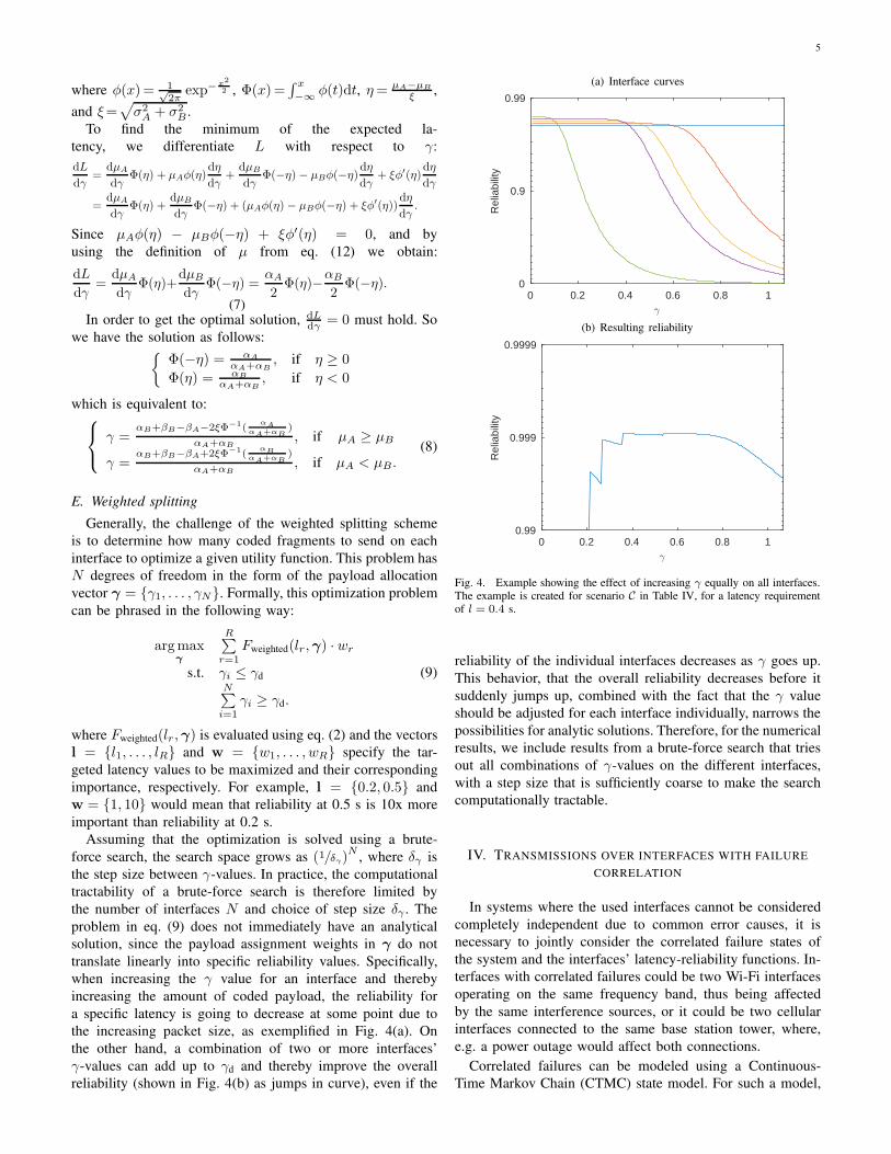
the increasing packet size, as exemplified in Fig. 4(a). On

the other hand, a combination of two or more interfaces’

γ-values can add up to γd and thereby improve the overall

reliability (shown in Fig. 4(b) as jumps in curve), even if the

(a) Interface curves

0 0.2 0.4 0.6 0.8 1γ

0.99

0.9

0

Rel

iabi

lity

(b) Resulting reliability

0 0.2 0.4 0.6 0.8 1γ

0.9999

0.999

0.99

Rel

iabi

lity

Fig. 4. Example showing the effect of increasing γ equally on all interfaces.The example is created for scenario C in Table IV, for a latency requirementof l = 0.4 s.

reliability of the individual interfaces decreases as γ goes up.

This behavior, that the overall reliability decreases before it

suddenly jumps up, combined with the fact that the γ value

should be adjusted for each interface individually, narrows the

possibilities for analytic solutions. Therefore, for the numerical

results, we include results from a brute-force search that tries

out all combinations of γ-values on the different interfaces,

with a step size that is sufficiently coarse to make the search

computationally tractable.

IV. TRANSMISSIONS OVER INTERFACES WITH FAILURE

CORRELATION

In systems where the used interfaces cannot be considered

completely independent due to common error causes, it is

necessary to jointly consider the correlated failure states of

the system and the interfaces’ latency-reliability functions. In-

terfaces with correlated failures could be two Wi-Fi interfaces

operating on the same frequency band, thus being affected

by the same interference sources, or it could be two cellular

interfaces connected to the same base station tower, where,

e.g. a power outage would affect both connections.

Correlated failures can be modeled using a Continuous-

Time Markov Chain (CTMC) state model. For such a model,

6

we calculate the combined latency-reliability function as:

Fm-dep(x,B) =

L∑

s=1

πs ·Hs(x,B), (10)

where L is the number of states in the CTMC, πs is the

steady-state probability of state s in the CTMC, and Hs(x,B)characterizes the latency-reliability function of state s.

Since the latency-reliability function Hs(x,B) associated

with a given system state s depends on the actual transmission

strategy, we will in following consider a specific case study

from which it becomes clear how Hs(x,B) is computed.

A. Case study: Correlated failures in three-interface system

We assume that an M2M device in Fig. 1 (b) is connected

with Wi-Fi to a fiber connection and by two cellular interfaces,

denoted by C1 and C2. This is an example of a mission

critical MTC use case from smart grid systems [25]. If the

cellular interfaces C1 and C2 belong to the same operator,

then they are likely located at the same base station tower,

such that we need to take into account the probability of

the cellular links failing simultaneously due to common error

causes. The CTMC in Fig. 5 shows the different modes of

operation considered for the case study. In addition to the

independent failures of C1, C2, and W-Fi the model also

includes BS failures. In states with BS failure, namely states

5, 8, 10, 11, 13, 14, 15, and 16, neither of the two cellular

interfaces will be functioning, since the BS failure represents

the common error causes that affect both cellular connections,

such as power outage or backhaul connection problems. We

need to specifically address the degenerate cases of states 11,

12, 14, 15, and 16 when nothing is functioning. While the

presented failure model is quite simple and only considers the

mentioned four high-level failures. This is however sufficient

for the needs of this analysis, since the model can be used

to determine the most suitable transmission strategy for a

certain system configuration and answer what-if questions

when having different probabilities of failure correlations.

For each of the considered transmission strategies, we

present a short description and define the state-specific latency-

reliability functions Hs(x,B) for s = 1, 2, . . . , L that are

represented by the vector H(x,B). For compact notation of

interface-specific latency-reliability functions, we let i = 1represents C1, i = 2 is C2, and i = 3 is Wi-Fi. Further,

we define that Fi = Fi(x, γiB)/Ai is the latency-reliability

function normalized by the availability Ai, thereby making Fi

a CDF. We do this because we have used Ai = 1−P(i)e in the

parametrization of the CTMC model. By normalizing Pe out of

the latency-reliability function and including it in the CTMC

we enable the use of probability theory for the following

analysis. The value of γi depends on the transmission strategy

used, as specified in Table I. Illustrations of the strategies

and packet size splitting parameters γi, are shown in Table

I and they are explained in the next section. Note that the

CTMC failure model in Fig. 5 is used with all three strategies,

since we assume that equipment and transmission failures are

independent of the used transmission strategy.

TABLE IPACKET SPLITTING PARAMETER FOR DIFFERENT STRATEGIES

cloning 2-of-3 weighted

γ1 1 1/2 · γd variableγ2 1 1/2 · γd 1−γ1γ3 1 1/2 · γd 1

1

All OK

3

C2

fail

2

C1

fail

4

Wi

fail

5

BS

fail

7

C1+Wi

fail

6

C1+C2

fail

8

C1+BS

fail

9

C2+Wi

fail

10

C2+BS

fail

11

Wi+BS

fail

12

C1+C2+Wi

fail

13

C1+C2+BS

fail

14

C1+Wi+BS

fail

15

C2+Wi+BS

fail

16

C1+C2+Wi+

BS fail

C1

C2

Wi

BS

C2

Wi

BS

C1

Wi

BS

C1

C2

BS

C1

C2

Wi

Wi

BS

C2

BS

C2

Wi

C1

BS

C1

Wi

C1

C2

BS

Wi

C2

C1

Fig. 5. CTMC model of states in the three interface system. Colors indicatethe number of interfaces up/down as: Green: 3/0, yellow: 2/1, orange: 1/2, red:0/3. An arrow represents a failure rate in the right direction and restorationrate in the left direction, e.g., λC1 and µC1 between states 1 and 2.

B. Packet cloning on three interfaces

For each state in Fig. 5, we need to specify how the

interfaces’ latency-reliability functions Fi(x,B) should be

combined. In states where more than one interface is avail-

able, the latency is given by the first arriving packet when

using cloning. Let the independent Random Variables (RVs)

X1, ..., Xk represent the latency of each of the m ∈ {1, 2, 3}interfaces. The latency CDF of the first arriving is known to

be Fmin = 1−Πmj=1(1−Fj). Thus, the Fi(x,B) functions are

combined as shown in Table II in order to obtain Hs(x,B)for all 16 states. The resulting latency-reliability function is

computed using (10).

C. 2-of-3 packet splitting on three interfaces

As explained in sec. II-A, a 2-out-of-3 strategy requires

only coded packets corresponding to 1/2 · γd of the source

packet to be sent on each interface. Consequently, the state-

specific latency-reliability functions are different from the ones

in packet cloning. In state 1, to compute the probability of

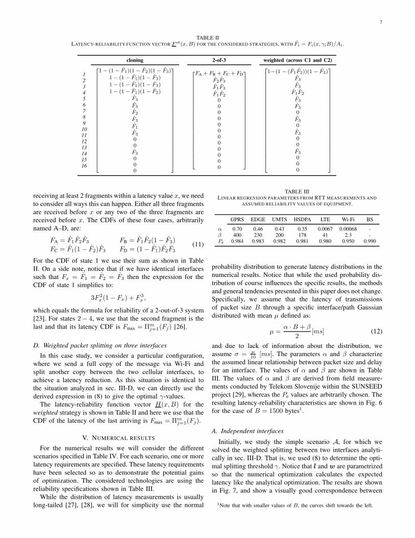
7

TABLE IILATENCY-RELIABILITY FUNCTION VECTOR F st(x,B) FOR THE CONSIDERED STRATEGIES, WITH Fi = Fi(x, γiB)/Ai .

cloning 2-of-3 weighted (across C1 and C2)

1

2

3

4

5

6

7

8

9

10

11

12

13

14

15

16

1− (1 − F1)(1− F2)(1 − F3)

1− (1 − F1)(1 − F3)

1− (1 − F1)(1 − F3)

1− (1 − F1)(1 − F2)

F3

F3

F2

F3

F1

F3

00

F3

000

FA + FB + FC + FD

F2F3

F1F3

F1F2

000000000000

1−(1 − (F1F2))(1 − F3)

F3

F3

F1F2

F3

F3

0

F3

0

F3

00

F3

000

receiving at least 2 fragments within a latency value x, we need

to consider all ways this can happen. Either all three fragments

are received before x or any two of the three fragments are

received before x. The CDFs of these four cases, arbitrarily

named A–D, are:

FA = F1F2F3 FB = F1F2(1− F3)

FC = F1(1 − F2)F3 FD = (1− F1)F2F3(11)

For the CDF of state 1 we use their sum as shown in Table

II. On a side note, notice that if we have identical interfaces

such that Fx = F1 = F2 = F3 then the expression for the

CDF of state 1 simplifies to:

3F 2x (1− Fx) + F 3

x ,

which equals the formula for reliability of a 2-out-of-3 system

[23]. For states 2− 4, we use that the second fragment is the

last and that its latency CDF is Fmax = Πmj=1(Fj) [26].

D. Weighted packet splitting on three interfaces

In this case study, we consider a particular configuration,

where we send a full copy of the message via Wi-Fi and

split another copy between the two cellular interfaces, to

achieve a latency reduction. As this situation is identical to

the situation analyzed in sec. III-D, we can directly use the

derived expression in (8) to give the optimal γ-values.

The latency-reliability function vector H(x,B) for the

weighted strategy is shown in Table II and here we use that the

CDF of the latency of the last arriving is Fmax = Πmj=1(Fj).

V. NUMERICAL RESULTS

For the numerical results we will consider the different

scenarios specified in Table IV. For each scenario, one or more

latency requirements are specified. These latency requirements

have been selected so as to demonstrate the potential gains

of optimization. The considered technologies are using the

reliability specifications shown in Table III.

While the distribution of latency measurements is usually

long-tailed [27], [28], we will for simplicity use the normal

TABLE IIILINEAR REGRESSION PARAMETERS FROM RTT MEASUREMENTS AND

ASSUMED RELIABILITY VALUES OF EQUIPMENT.

GPRS EDGE UMTS HSDPA LTE Wi-Fi BS

α 0.70 0.46 0.43 0.35 0.0067 0.00068 -β 400 230 200 178 41 2.3 -Pe 0.984 0.983 0.982 0.981 0.980 0.950 0.990

probability distribution to generate latency distributions in the

numerical results. Notice that while the used probability dis-

tribution of course influences the specific results, the methods

and general tendencies presented in this paper does not change.

Specifically, we assume that the latency of transmissions

of packet size B through a specific interface/path Gaussian

distributed with mean µ defined as:

µ =α · B + β

2[ms] (12)

and due to lack of information about the distribution, we

assume σ = µ10 [ms]. The parameters α and β characterize

the assumed linear relationship between packet size and delay

for an interface. The values of α and β are shown in Table

III. The values of α and β are derived from field measure-

ments conducted by Telekom Slovenije within the SUNSEED

project [29], whereas the Pe values are arbitrarily chosen. The

resulting latency-reliability characteristics are shown in Fig. 6

for the case of B = 1500 bytes1.

A. Independent interfaces

Initially, we study the simple scenario A, for which we

solved the weighted splitting between two interfaces analyti-

cally in sec. III-D. That is, we used (8) to determine the opti-

mal splitting threshold γ. Notice that l and w are parametrized

so that the numerical optimization calculates the expected

latency like the analytical optimization. The results are shown

in Fig. 7, and show a visually good correspondence between

1Note that with smaller values of B, the curves shift towards the left.

8

TABLE IVINTERFACE AND PARAMETER SPECIFICATIONS OF SCENARIOS A, B, C , AND D.

IF1 IF2 IF3 IF4 IF5 B l w

A Wi-Fi UMTS GPRS - - 1500 bytes [0 . . . 1] s [0 . . . 1]B Wi-Fi UMTS EDGE GPRS - 3500 bytes [0.7] s [1]C LTE HSDPA UMTS EDGE GPRS 1500 bytes [0.1, 0.4, 0.9∗] s [1, 10, 100∗]D HSDPA HSDPA GPRS GPRS GPRS 1500 bytes [0.5] s [1]E Wi-Fi UMTS EDGE - - 1500 bytes [0 . . . 1] s [0 . . . 1]

0 0.2 0.4 0.6 0.8 1 1.2 1.4

Latency (x)

0.99

0.9

0

F(x

) Wi-Fi

LTE

HSDPA

UMTS

EDGE

GPRS

Fig. 6. Latency-reliability curves Fi(x,B) for all considered technologiesfor B = 1500 bytes.

the analytical result and the brute-force search. The brute-force

search has a slightly lower expected latency, due to the weight

assignment being different. We attribute this minor difference

to the use of the approximation of E[max(XA, XB)] from

[24].

0 0.2 0.4 0.6 0.8 1

Latency (x)

0.9999

0.999

0.99

0.9

0

Rel

iabi

lity

1-of-3 =[1.0533 1.0533 1.0533], i = 3.16

2-of-3 =[0.52667 0.52667 0.52667], i = 1.58

3-of-3 =[0.35333 0.35333 0.35333], i = 1.06

Weighted (brute-force): =[1.0667 0.8 0.26667], i = 2.1333

Weighted (analytic): 1.0667 0.84962 0.21705, i = 2.1333

Fig. 7. Reliability results for scenario A.

In relation to the general idea of splitting, the most im-

portant question we seek to answer, is if it makes sense to

spend the additional effort required to find the optimal γ-

values for a weighted splitting or if it suffices to use one of

the simpler k-out-of-N strategies. It is intuitively clear that

if the used technologies are all identical, then a k-out-of-Nstrategy will be optimal. But how much better is a weighted

scheme in a heterogeneous scenario? To answer this we study

three different scenarios that are specified in Table IV.

The resulting reliabilities for the different transmission

strategies are shown for scenario B in Fig. 8. The most

distinctive observation is that in the low latency region x <0.3 s, only the 1-out-of-4 and Weighted strategies provide

any reliability. However, around the target latency x = 0.7 s,

both the 2-out-of-4 and 1-out-of-4 strategies achieve higher

reliability than the 1-out-of-4 since the payload is split between

the interfaces. Nevertheless, the optimal weight assignment

used by the Weighted strategy has the highest reliability at

x = 0.7 s. The assigned γ-values are shown in the figure

legend. In comparison to the 1-out-of-4 (Cloning) strategy we

see a significant improvement in reliability from 0.95 to 0.997

at the target latency x = 0.7 s. In terms of latency, at R=0.997,

we see a reduction from 1.05 s to 0.7 s.

0 0.2 0.4 0.6 0.8 1 1.2 1.4

Latency (x)

0.9999

0.999

0.99

0.9

0

Rel

iabi

lity

1-of-4 =[1.0514 1.0514 1.0514 1.0514], i = 4.2057

2-of-4 =[0.52571 0.52571 0.52571 0.52571], i = 2.1029

3-of-4 =[0.35143 0.35143 0.35143 0.35143], i = 1.4057

4-of-4 =[0.26286 0.26286 0.26286 0.26286], i = 1.0514

Weighted (brute-force): =[1.0571 0.4 0.2 0.45714], i = 2.1143

Fig. 8. Reliability results for scenario B.

While scenario B demonstrated how latency can be lowered,

the results for scenario C in Fig. 9 show two examples of

latency-reliability trade-offs that are achieved by considering

both when the starred l and w values in Table IV are included

and excluded. In both cases the weighted strategy achieves

some reliability in the low latency region (x < 0.2 s) similar

to the 1-out-of-5 strategy and it has the reliability of the 2-

out-of-5 strategy around x = 0.4 s. The difference between

the 2 results is that the last one transmits more redundancy

data and achieves higher reliability in the x > 0.4 s region.

The last results concerning scenario D that are shown in

Fig. 10 are interesting since they demonstrate a more mixed

data allocation. This results in the reliability at x = 0.5 s

being 0.9999, which is one decade better than any k-out-of-Nstrategy that only go up to 0.999.

9

0 0.1 0.2 0.3 0.4 0.5 0.6 0.7 0.8 0.9 1

Latency (x)

0.999999999

0.99999999

0.9999999

0.999999

0.99999

0.9999

0.999

0.99

0.9

0

Rel

iabi

lity

1-of-5 γ=[1.0533 1.0533 1.0533 1.0533 1.0533], Σ γi = 5.2667

2-of-5 γ=[0.52667 0.52667 0.52667 0.52667 0.52667], Σ γi = 2.6333

3-of-5 γ=[0.35333 0.35333 0.35333 0.35333 0.35333], Σ γi = 1.7667

4-of-5 γ=[0.26667 0.26667 0.26667 0.26667 0.26667], Σ γi = 1.3333

5-of-5 γ=[0.21333 0.21333 0.21333 0.21333 0.21333], Σ γi = 1.0667

Weighted (brute-force): γ=[1.0667 0.66667 0.53333 0.4 0.13333], Σ γi = 2.8

Weighted (brute-force): γ=[1.0667 0.53333 0.53333 0.53333 0.53333], Σ γi = 3.2

Fig. 9. Reliability results for scenario C. Note: the target latency l2 = 0.9 sonly applies to the last strategy.

TABLE VCASE STUDY FAILURE AND RESTORATION RATES

λ (f/week) µ (r/week)

Wi-Fi + Fiber (Wi) 1.47 28 (6 hrs/r)Cellular (C1, C2) 0.64 50.4 (200 min/r)Base station (BS) 0.76 50.4 (200 min/r)

B. Interfaces with failure correlation

For this case study, we consider that besides failing inde-

pendently, C1 and C2 can also fail simultaneously due to a

common BS failure. This will be reflected in the MC model

results, whereas the independent results do not account for

common cause failures.

For evaluating the resulting performance of the considered

transmission modes, actual data on Mean Time to Restora-

tion (MTTR) and availability levels of different technologies

has been used. From these numbers, the unspecified failure

and restoration rates have been determined. The approach to

parametrize the CTMC model is explained in the Appendix.

Table V presents the used failure and restoration rates.

With failure and restoration rates fully specified, the re-

sulting latency-reliability performance is calculated using the

methods outlined in sec. III. The different model results

have been verified using Matlab-based simulation. We first

simulated the transitions between states in the CTMC model

in Fig. 5 with exponential sojourn times given from the rates

in Table V. Hereafter we replayed the state sequence and for

every 1 min simulation time, a random Gaussian latency value

was drawn for the interfaces available in the current state.

0 0.1 0.2 0.3 0.4 0.5 0.6 0.7 0.8 0.9 1Latency (x)

0.9999999

0.999999

0.99999

0.9999

0.999

0.99

0.9

0

Rel

iabi

lity

1-of-5 γ=[1.0533 1.0533 1.0533 1.0533 1.0533], Σ γi = 5.2667

2-of-5 γ=[0.52667 0.52667 0.52667 0.52667 0.52667], Σ γi = 2.6333

3-of-5 γ=[0.35333 0.35333 0.35333 0.35333 0.35333], Σ γi = 1.7667

4-of-5 γ=[0.26667 0.26667 0.26667 0.26667 0.26667], Σ γi = 1.3333

5-of-5 γ=[0.21333 0.21333 0.21333 0.21333 0.21333], Σ γi = 1.0667

Weighted (brute-force): γ=[0.8 0.8 0.26667 0.4 0.4], Σ γi = 2.6667

Fig. 10. Reliability results for scenario D.

Depending on the required packet fragments of the strategy

either a transmission latency or timeout value resulted. The

CDF of these values is shown with crosses in Fig. 11.

0 0.1 0.2 0.3 0.4 0.5 0.6 0.7 0.8 0.9 1

Latency (x)

0.9999

0.999

0.99

0.9

0

Rel

iabi

lity

Cloning (independent)Cloning (MC model)2-of-3 (independent)2-of-3 (MC model)Weighted (independent)Weighted (MC model)

Fig. 11. Reliability results for scenario E , where we found γ = 0.55.

In all plots in Fig. 11 we see that the Cloning strategy,

which uses three times as much bandwidth as a single-

interface transmission, achieves the highest reliability in the

high latency region. The impact of failure correlations is shown

from the difference between the independent and MC model

curves. For cloning, the difference amounts to more than one

decade at high latency values. This difference results from

the fact that both cellular interfaces are depending on the

base station being operational. That is, in cases where the

base station fails (model states: 5, 8, 10, 11, 13, 14, 15, 16)

10

neither C1 or C2 will be operational. 2 The 2-out-of-3 strategy

uses only half the total bandwidth of cloning. However, the

dependence on at least two working interfaces causes the lack

of reliability before 0.2 s. While in the independent case the

2-out-of-3 strategy is able to reduce latency up to almost

0.9 s at R = 0.996, the MC model result that accounts

for correlated failures, is the worst strategy, except the small

interval 0.35 − 0.42 s where it reaches the same reliability

level as cloning. Finally, the Weighted strategy shows the best

performance for low latency (x ≤ 0.5 s), whereas it is only

slightly worse than Cloning (independent) for higher latency

values. It is worth noticing that the difference between the

independent and MC model results for this strategy is minimal.

We explain this from the fact that in the weighted strategy the

cellular interfaces are inherently depending on each other also

in the independent case, whereas for cloning and 2-out-of-3,

the two cellular interfaces are independent in the independent

case, but dependent when using the MC model.

Besides considering only the level of reliability that each

strategy can achieve, we are showing also the efficiency as

the achieved reliability (in number of nines) in relation to

the amount of coded data transmitted (B bytes) in Fig. 12.

While the independent results show that both the 2-out-of-3

and cloning strategies are better than the weighted strategy,

this observation does not hold for the case with correlated

failures (MC model). In this case the weighted strategy is the

best choice for the whole span of latency values.

0 0.1 0.2 0.3 0.4 0.5 0.6 0.7 0.8 0.9 1

Latency (x)

0

0.2

0.4

0.6

0.8

1

1.2

1.4

1.6

1.8

2

Effi

cien

cy: n

ines

per

B u

sed

Cloning (independent)Cloning (MC model)2-of-3 (independent)2-of-3 (MC model)Weighted (independent)Weighted (MC model)

Fig. 12. Efficiency results for scenario E .

C. Experimental validation

In addition to the theoretical and model-based results pre-

sented above, we have also validated the proposed method

for combining the latency-reliability functions using exper-

imental results. While this validation experiment does not

explicitly cover all of the scenarios A-E , it shows how well

the latency-reliability curves can be used to calculate the

actual performance of multi-interface transmissions. In the

experiment, we have used traces of latency measurements

for different communication technologies. Such traces were

obtained by sending small (128 bytes) UDP packets every

2The used value of Pe = 0.99 for the base station may be high comparedto a real-life system, however the main point of the analysis is to show howsuch factors can be modeled.

(a)

1 2 5 10 20 50 100l [ms]

0.9999

0.999

0.99

0.9

0

LTEHSPAWi-Fi

(b)

1 2 5 10 20 50 100l [ms]

0.9999

0.999

0.99

0.9

0

1-out-of-32-out-of-33-out-of-3

Fig. 13. (a) Interfaces’ latency-reliability curves. Wi-Fi is IEEE 802.11n.(b) Resulting performance of considered strategies. Lines show the resultscomputed using the method presented in sec. III, crosses show the results ofplayback-simulation.

100 ms between a pair of GPS time-synchronized devices

through the considered interface (LTE, HSPA, or Wi-Fi) during

the course of a work day at Aalborg University campus. Each

trace file can thus be used to play back a time sequence of one-

way end-to-end latencies. Our experimental results of multi-

interface transmissions are obtained by playing back the three

trace files at the same time time in a simulation, where for

every 100 ms, the outcome of each considered strategy is

recorded. When the simulation is done, a latency-reliability

curve is calculated for each strategy as the cdf of the recorded

outcomes in each 100 ms timestep. This is shown with crosses

in Fig. 13 (b). The validation consists in comparing these

results to the results that are obtained by using the curves in

Fig. 13 (a) to compute the resulting latency-reliability curves

using the methods described in sec. III. Those results are

shown as lines in Fig. 13 (b).

From the results in Fig. 13, we see how the 1-out-of-3

strategy is able to outperform any individual interface, as

expected. The plot does not include any result for the Weighted

scheme, since the small payload size does not allow for any

gain through payload splitting. The lines that represent the

theoretical calculation of performance are practically coin-

ciding with the crosses representing the experimental results.

This shows that the methods for calculating the resulting

performance by relying on the latency-reliability curves of the

interfaces, as described in Sec. III, indeed produces accurate

results when used with actual traffic traces.

11

VI. CONCLUSIONS AND OUTLOOK

It is expected that 5G will integrate various communica-

tion technologies to support ultra-reliable and low latency

(URLLC) use cases. In this work we denote this integration

interface diversity and consider different strategies for utilizing

multiple interfaces simultaneously, to achieve high reliability

and low latency. By flexibly allocating coded fragments of

the encoded payload message to different interfaces, according

to their bit-rate, latency and reliability properties, it becomes

possible to trade-off transmission latency and reliability. We

have considered both static k-out-of-n strategies and optimized

weighted strategies.

For evaluating performance, we have proposed an analysis

framework that combines traditional reliability models with

technology-specific latency probability distributions. The pro-

posed models can be used both for systems with independently

failing communication paths and for systems with common

error causes, e.g. if cellular technologies reside in the same

base station tower.

Our main findings are that 1) interface diversity strategies

can lower the latency up to around 40% in practical systems

when large messages are transmitted using low rate technolo-

gies, where the time to transmit the bits over the air is substan-

tial in relation to the access delay; 2) in some cases only the

optimized weighted strategy (and not the simple k-out-of-n)

can deliver latency reduction and reliability at low latencies;

3) the optimized weighted strategy enables the fine-tuning of

the latency-reliability trade-off for a specific scenario; and

4) we have experimentally validated the proposed method

of computing the resulting performance, and demonstrated

the practical gains of interface diversity in a three interface

scenario for the k-out-of-n strategies.

ACKNOWLEDGMENT

This work is partially funded by EU, under Grant agreement

no. 619437. The SUNSEED project is a joint undertaking

of 9 partner institutions and their contributions are fully

acknowledged. The work was also supported in part by the

European Research Council (ERC Consolidator Grant no.

648382 WILLOW) within the Horizon 2020 Program.

Also, thanks to Kasper F. Trillingsgaard for constructive

comments and suggestions.

APPENDIX

This appendix explains the approach used to determine the

Markov chain failure and restoration rates for the dependent

cellular technologies C1 and C2. For this, we consider the

CTMC model corresponding to the cellular subsystem of Fig.

1 (b). This subsystem is shown in Fig. 14.

Initially, we specify the known individual availabilities AC1

and AC2 as well as the known base station availability ABS,

given in Table V. Transitions between states are specified by

the failure rates denoted by λ and restoration rates denoted

by µ. Notice that neither failure rates or restoration rates are

known for the considered case study. We have therefore made

assumptions in the values of the restoration rates as specified

in Table V.

1

All OK

3

C2

fail

2

C1

fail

4

BS

fail

5

C2+C1

fail

6

C1+BS

fail

7

C2+BS

fail

8

C1+C2+BS

fail

C1

C2

BS

C2

BS

C1

BS

C1

C2

BS

C2

C1

Fig. 14. State-transition diagram of the continuous time Markov chain thatrepresents the cellular connections C1 and C2 with correlated failures.

Given the availabilities AC1, AC2, and ABS, we determine

the state probabilities πi of the states in Fig. 14, by solving

the following linear equation system that explains the relations

between the steady state probabilities and availability proba-

bilities:

1 0 1 1 0 0 1 01 1 0 1 0 1 0 01 1 1 0 1 0 0 00 1 −1 0 0 0 0 00 0 0 0 1 −1 0 00 0 0 0 0 1 0 00 0 0 0 0 0 1 00 0 0 0 0 0 0 11 1 1 1 1 1 1 1

π1

π2

π3

π4

π5

π6

π7

π8

=

A1

A2

ABS

00

AC1ABS

AC2ABS

AC1AC2ABS

1

,

where A∗ = 1−A∗ is used for compact notation.

Having obtained the state probabilities π = [π1 . . . π5],we set up the following balance equations that explain the

relations between the failure and restoration rates according

to Fig. 14. The assumed mean restoration rates in Table V are

given as input and we can then solve the corresponding linear

system:

−π1 −π1 −π1 π2 π3 π4

π1 −π2 −π2 −π2 π4 π5

−π3 π1 −π3 π4 −π3 π5

−π4 −π4 π1 π6 π7 −π4

π3 π2 −π5 −π5 −π5 π8

π4 −π6 π2 −π6 π8 −π6

−π7 π4 π3 π8 −π7 −π7

π7 π6 π5 −π8 −π8 −π8

−1 1 0 0 0 00 0 0 −1 1 00 0 0 1 0 00 0 0 0 1 00 0 0 0 0 1

λC1

λC2

λBS

µC1

µC2

µBS

=

0000000000µC1

µC2

µBS

.

Thereby we obtain a set of failure rates λC1, λC2, and λBS

that satisfy the constraints of the system in terms of state

probabilities, restoration rates, and balance relations between

states.

12

REFERENCES

[1] E. De Carvalho, E. Bjornson, J. H. Sorensen, P. Popovski, and E. G.Larsson, “Random access protocols for massive mimo,” IEEE Commu-

nications Magazine, vol. 55, no. 5, pp. 216–222, 2017.

[2] H. Ji, S. Park, J. Yeo, Y. Kim, J. Lee, and B. Shim, “Introduction toultra reliable and low latency communications in 5g,” arXiv preprint

arXiv:1704.05565, 2017.

[3] J. G. Andrews, S. Buzzi, W. Choi, S. V. Hanly, A. Lozano, A. C. Soong,and J. C. Zhang, “What will 5g be?” Selected Areas in Communications,

IEEE Journal on, vol. 32, no. 6, pp. 1065–1082, 2014.

[4] J. F. Monserrat, G. Mange, V. Braun, H. Tullberg, G. Zimmermann, andO. Bulakci, “Metis research advances towards the 5g mobile and wirelesssystem definition,” EURASIP Journal on Wireless Communications and

Networking, vol. 2015, no. 1, pp. 1–16, 2015.

[5] R. Ratasuk, A. Prasad, Z. Li, A. Ghosh, and M. Uusitalo, “Recentadvancements in m2m communications in 4g networks and evolutiontowards 5g,” in Intelligence in Next Generation Networks (ICIN), 2015

18th International Conference on. IEEE, 2015, pp. 52–57.

[6] E. Lahetkangas, K. Pajukoski, J. Vihriala, G. Berardinelli, M. Lauridsen,E. Tiirola, and P. Mogensen, “Achieving low latency and energy con-sumption by 5g tdd mode optimization,” in Communications Workshops

(ICC), 2014 IEEE International Conference on. IEEE, 2014, pp. 1–6.

[7] H. Tullberg, Z. Li, A. Hoglund, P. Fertl, D. Gozalvez-Serrano,K. Pawlak, P. Popovski, G. Mange, and O. Bulakci, “Towards the METIS5G concept: First view on horizontal topics concepts,” in Networks and

Communications (EuCNC), European Conf. on. IEEE, 2014, pp. 1–5.

[8] 3GPP, “3gpp tr 36.881 v0.6.0: Evolved universal terrestrial radio access(e-utra); study on latency reduction techniques for lte (release 13),” Tech.Rep., Feb 2016.

[9] E. Dahlman, G. Mildh, S. Parkvall, J. Peisa, J. Sachs, and Y. Selen, “5gradio access,” Ericsson Review, vol. 6, pp. 2–7, 2014.

[10] J. Qadir, A. Ali, K.-L. A. Yau, A. Sathiaseelan, and J. Crowcroft,“Exploiting the power of multiplicity: a holistic survey of network-layermultipath,” IEEE Communications Surveys & Tutorials, vol. 17, no. 4,pp. 2176–2213, 2015.

[11] J. G. Apostolopoulos, “Reliable video communication over lossy packetnetworks using multiple state encoding and path diversity,” in Photonics

West 2001-Electronic Imaging. International Society for Optics andPhotonics, 2000, pp. 392–409.

[12] K.-K. Yap, T.-Y. Huang, M. Kobayashi, Y. Yiakoumis, N. McKeown,S. Katti, and G. Parulkar, “Making use of all the networks around us:A case study in android,” in Proceedings of the 2012 ACM SIGCOMM

Workshop on Cellular Networks: Operations, Challenges, and Future

Design, ser. CellNet ’12. New York, NY, USA: ACM, 2012, pp. 19–24.[Online]. Available: http://doi.acm.org/10.1145/2342468.2342474

[13] K.-K. Yap, T.-Y. Huang, Y. Yiakoumis, S. Chinchali, N. McKeown, andS. Katti, “Scheduling packets over multiple interfaces while respectinguser preferences,” in Proceedings of the Ninth ACM Conference on

Emerging Networking Experiments and Technologies, ser. CoNEXT’13. New York, NY, USA: ACM, 2013, pp. 109–120. [Online].Available: http://doi.acm.org/10.1145/2535372.2535387

[14] S. Singh, S.-p. Yeh, N. Himayat, and S. Talwar, “Optimal traffic aggrega-tion in multi-rat heterogeneous wireless networks,” in Communications

Workshops (ICC), 2016 IEEE International Conference on. IEEE, 2016,pp. 626–631.

[15] D. S. Michalopoulos, I. Viering, and L. Du, “User-plane multi-connectivity aspects in 5g,” in Telecommunications (ICT), 2016 23rd

International Conference on. IEEE, 2016, pp. 1–5.

[16] A. Ravanshid, P. Rost, D. S. Michalopoulos, V. V. Phan, H. Bakker,D. Aziz, S. Tayade, H. D. Schotten, S. Wong, and O. Holland, “Multi-connectivity functional architectures in 5g,” in Communications Work-

shops (ICC), 2016 IEEE International Conference on. IEEE, 2016, pp.187–192.

[17] A. Wolf, P. Schulz, D. Ohmann, M. Dorpinghaus, and G. Fettweis,“Diversity-multiplexing tradeoff for multi-connectivity and the gain ofjoint decoding,” arXiv preprint arXiv:1703.09992, 2017.

[18] J. J. Nielsen and P. Popovski, “Latency analysis of systems withmultiple interfaces for ultra-reliable m2m communication,” in Signal

Processing Advances in Wireless Communications (SPAWC), 2016 IEEE

17th International Workshop on. IEEE, 2016, pp. 1–6.

[19] J. J. Nielsen, R. Liu, and P. Popovski, “Latency-optimized interfacediversity for ultra-reliable low latency communication (URLLC),” Ac-

cepted for IEEE Globecom’17, 2017.

[20] E. G. Strom, P. Popovski, and J. Sachs, “5g ultra-reliable vehicularcommunication,” arXiv preprint arXiv:1510.01288, 2015.

[21] D. J. MacKay, “Fountain codes,” IEE Proceedings-Communications, vol.152, no. 6, pp. 1062–1068, 2005.

[22] S. B. Wicker and V. K. Bhargava, Reed-Solomon codes and their

applications. John Wiley & Sons, 1999.[23] M. Rausand and A. Høyland, System reliability theory: models, statis-

tical methods, and applications. John Wiley & Sons, 2004, vol. 396.[24] C. E. Clark, “The greatest of a finite set of random variables,” Operations

Research, vol. 9, no. 2, pp. 145–162, 1961.[25] C. Stefanovic, P. Popovski, L. Jorguseski, and R. Sernec, “SUNSEED–an

evolutionary path to smart grid comms over converged telco and energyprovider networks,” in Wireless Communications, Vehicular Technology,

Information Theory and Aerospace & Electronic Systems (VITAE), 2014

4th International Conference on. IEEE, 2014, pp. 1–5.[26] S. M. Ross et al., Stochastic processes. John Wiley & Sons New York,

1996, vol. 2.[27] M. S. Borella, S. Uludag, G. B. Brewster, and I. Sidhu, “Self-similarity

of internet packet delay,” in Communications, 1997. ICC’97 Montreal,

Towards the Knowledge Millennium. 1997 IEEE International Confer-

ence on, vol. 1. IEEE, 1997, pp. 513–517.[28] J. A. Jacko, A. Sears, and M. S. Borella, “The effect of network

delay and media on user perceptions of web resources,” Behaviour &

Information Technology, vol. 19, no. 6, pp. 427–439, 2000.[29] SUNSEED FP7 project. [Online]. Available: http://sunseed-fp7.eu/