Money and Banking: Some DSGE Challenges

Harald Uhlig∗

University of Chicago, CentER, NBER and CEPR

PRELMINARY

COMMENTS WELCOME

First draft: May 6th, 2018This revision: May 10, 2018

Abstract

DSGE models were meant to rise to the Lucas (1976) challenge

of constructing general equilibrium models with deep parameters, to

be used as workhorse models for e.g. monetary policy analysis. But

challenges remain. This paper discusses a few of them. The central

issue of the impact of monetary policy on yield spreads and asset

prices is often ignored in DSGE models or kept essential separate

from allocations. While much progress has been made on considering

financial frictions in DSGE models, the models need to allow more

room for private markets to address these frictions, rather than call

∗This paper was written for the Nobel Symposium on “Money and Banking”, Stock-

holm, May 26-28, 2018. Address: Harald Uhlig, Department of Economics, University of

Chicago, 1126 East 59th Street, Chicago, IL 60637, U.S.A, email: huhlig@uchicago.edu.

I have an ongoing consulting relationship with a Federal Reserve Bank, the Bundesbank

and the ECB.

on economic policy. The Phillips-Curve tradeoff, so central to thinking

about monetary policy and much of the DSGE literature, may hardly

be there. New Keynesian models, which have largely become the

benchmark approach to thinking about monetary policy in central

banks, have strong, but often-ignored neo-Fisherian properties. In

sum, the glass is half full. Or half empty. Take your pick.

Keywords: DSGE models, Monetary Policy, asset prices, financial fric-

tions, Phillips curve, New Keynesian, Neo-Fisherian

2

The purpose of this paper is to provide a bit of a birds-eye perspective

and critique of the DSGE approach to thinking about monetary policy and

banking. I will pick out a few points or challenges only, in the interest of

length. I admit that the selection of these particular challenges are partly

driven by a desire of expositing some of my own work. There are many more

which could (and perhaps should) be added. The title of this paper may

share some similarities with the title of Linde et al (2016), though the per-

spective differs considerably. Instead, this paper is perhaps closer in spirit

to the perspective of Gilles Saint-Paul (2018), who provides a more formal

modelling of the concerns raised here, or the skepticism towards the con-

ventional empirical identification of monetary policy shocks in Uhlig (2005)

or the skepticism regarding the effectiveness of monetary policy to influence

employment, see McGrattan (2015).

Dynamic stochastic general equilibrium or DSGE models were meant to

rise to the Lucas (1976) challenge of constructing general equilibrium models

with deep parameters, to be used as workhorse models for e.g. monetary

policy analysis. Indeed, the last two decades have witnessed a remarkably

successful epoch for this approach, with quantitative New Keynesian mod-

els such as Smets-Wouters (2007) being increasingly at the heart of mone-

tary policy discussions in central banks. Likewise, though at a considerably

slower speed, they have become of increasing relevance for macro-fiscal pol-

icy, in particular for thinking about fiscal multipliers and the impacts of

fiscal stimulus in times of economic crisis and zero-lower-bound constraints

on monetary policy, see e.g. Coenen et al. (2012) or Drautzburg-Uhlig (2015)

for some examples of that literature. The financial crises led to a substan-

tial recent literature of incorporating a variety of financial intermediaries and

financial frictions into models of these type, making the recent crop undoubt-

edly even more attractive, see e.g. Gertler et al (2016), Linde et al (2016) or

Wieland et al. (2016). Finally, DSGE models have become a highly useful

structural framework for thinking about and identifying frictions or wedges

and for guiding research towards still-missing parts of the theory, see Brinca

et al (2016).

One approach for me here would be to contribute yet another victory lap,

demonstrating the remarkable success of this branch of economic analysis.

At the very least, I could act as a cheerleader for the key recent contributors,

building that literature. I do applaud what they do, and going this route

was tempting indeed.

Instead, and with some trepidation, I shall point to some remaining chal-

lenges instead. This is slippery territory indeed. The literature is vast, and

it is impossible for some readers to not feel sleighted by the critique offered

here: their work may have just precisely addressed the issue raised here, and

it may be my fault entirely of having ignored it or not having presented it suf-

ficiently clearly, and it is my fault entirely of not being sufficiently informed

about the current frontier or not discussing these contributions with sufficient

care. Mea culpa. However, perhaps the critique here may then intead simply

to lead to a yet more concentrated effort of moving these contributions to

the forefront of the policy debates.

I shall discuss the following challenges in particular in greater detail in

the sections of this paper. The central issue of the impact of monetary policy

on yield spreads and asset prices is often ignored in DSGE models or kept

essentially separate from allocations, see section 1. Much progress has been

made for considering financial frictions in DSGE models. Yet, the models

need to allow more room for private markets to address these frictions, rather

than to call on economic policy, see section 2. The Phillips-Curve tradeoff, so

central to thinking about monetary policy and much of the DSGE literature,

may hardly be there, see section 3. New Keynesian models have neo-Fisherian

properties, but which are rarely advertised, see section 4. Hopefully, some of

these issues get addressed in future research. A constructive approach here

might be to apply the approach of Brinca et al (2016) and extend it to the

realm of asset pricing to provide a guide, beyond the specific challenges listed

here.

The final section 5 offers some summary and conclusions. In brief, it

2

seems to me that the glass is half full. Or half empty. Take your pick.

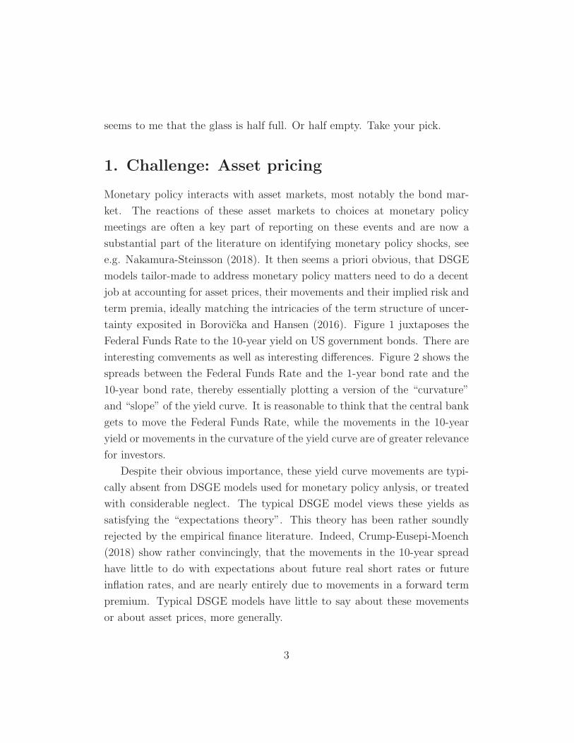
1. Challenge: Asset pricing

Monetary policy interacts with asset markets, most notably the bond mar-

ket. The reactions of these asset markets to choices at monetary policy

meetings are often a key part of reporting on these events and are now a

substantial part of the literature on identifying monetary policy shocks, see

e.g. Nakamura-Steinsson (2018). It then seems a priori obvious, that DSGE

models tailor-made to address monetary policy matters need to do a decent

job at accounting for asset prices, their movements and their implied risk and

term premia, ideally matching the intricacies of the term structure of uncer-

tainty exposited in Borovicka and Hansen (2016). Figure 1 juxtaposes the

Federal Funds Rate to the 10-year yield on US government bonds. There are

interesting comvements as well as interesting differences. Figure 2 shows the

spreads between the Federal Funds Rate and the 1-year bond rate and the

10-year bond rate, thereby essentially plotting a version of the “curvature”

and “slope” of the yield curve. It is reasonable to think that the central bank

gets to move the Federal Funds Rate, while the movements in the 10-year

yield or movements in the curvature of the yield curve are of greater relevance

for investors.

Despite their obvious importance, these yield curve movements are typi-

cally absent from DSGE models used for monetary policy anlysis, or treated

with considerable neglect. The typical DSGE model views these yields as

satisfying the “expectations theory”. This theory has been rather soundly

rejected by the empirical finance literature. Indeed, Crump-Eusepi-Moench

(2018) show rather convincingly, that the movements in the 10-year spread

have little to do with expectations about future real short rates or future

inflation rates, and are nearly entirely due to movements in a forward term

premium. Typical DSGE models have little to say about these movements

or about asset prices, more generally.

3

1940 1960 1980 2000 2020date

0

5

10

15

20

perc

ent

FFR vs 10-year yield

Figure 1: Yield Curves: FFR vs 10-year yields

1940 1960 1980 2000 2020date

-8

-6

-4

-2

0

2

4

perc

ent

1yr-FFR and 10yr-FFR yield spreads

Figure 2: Yield Spreads: 1 yr or 10 yr versus FFR.

4

Indeed, from the get-go, there is a skeleton in the closet of consumption-

based asset pricing, which is hardly, if ever addressed. For its most simple

variant, consider a log-linearized solution of some DSGE model for consump-

tion ct and the return Rt of some asset. Let xt denote the state of the

economy of date t. A recursive law of motion as constructed, say, with the

methods in Uhlig (1999) will then result in

log(ct+1) = log(c) + φxt + ǫt+1

log(Rt+1) = log(R) + ξxt + νt+1

for some steady state levels, coefficients φ, ξ as well as some possibly corre-

lated one-step ahead prediction errors ǫt+1 and νt+1. Assume log preferences,

discounted at β per period. The standard Lucas asset pricing equation, see

Lucas (1978), delivers

1 = Et

[

β

(

ct

ct+1

)

Rt+1

]

= βRcte(ξ−φ)stEt

[

eνt+1−ǫt+1

]

Suppose now, that the difference between the one step-ahead prediction er-

rors is normally distributed, νt+1 − ǫt+1 ∼ N (0, σ2t ), conditional on t. Then,

Et

[

eνt+1−ǫt+1

]

= eσ2t/2

Armed with this formula, one can now derive an expression for the risk

premium for the asset and its associated Sharpe ratio. This is exploited

frequently for examining asset premia or for the risk-adjustment of steady

states, see Lettau-Uhlig (2002), Schmitt-Grohe-Uribe (2004), Coeurdacier et

al (2011) or Uhlig (2018). But compare that to the situation, where that

difference has a student-t distribution with, say, 1000 degrees of freedom,

νt+1 − ǫt+1 ∼ t1000(0, σ2t ), conditional on t. Then,

Et

[

eνt+1−ǫt+1

]

=∞∑

j=0

1

j!Et

[

(νt+1 − ǫt+1)j]

=∞∑

j=0

1

(2j)!Et

[

(νt+1 − ǫt+1)2j]

= ∞

5

where I have exploited that a t−distribution is symmetric and eventually

has moments equal to infinity1. t−distributions and thus these infinities arise

rather naturally in an environment, where variables are normally distributed,

but agents need to learn about their variances, see Weitzman (2007). A plot

of the densities of the t−distribution chosen above relative to a normal dis-

tribution with equal mean and variance would not reveal much difference:

indeed, they would be hard to tell them apart in the data. But it is now

possible to generate infinite risk premia. Indeed, if one is free to choose any

distribution “between” the thin-tailed normal distribution and the fat-tailed

t−distribution, one can generate any desired risk premium. It should be

fairly clear, that the calculation does not rest on choosing log-preferences

in particular. It also seems plausible, that the argument does not rest on

the log-approximation per ser, but simply on the potentially fat tails of the

surprise component of log returns: indeed, a substantial layer of sophis-

ticated numerical approximation techniques may ultimately just obfuscate

these rather straightforward, but powerful insights. There is a large finance

literature documenting fat-tailed asset returns: if anything, a t−distribution

with 1000 degrees of freedom still errs on the side of caution.

One might draw the conclusion that the much-loved consumption-based

asset pricing theories, which are in turn at the core of DSGE modeling, do not

offer us much guidance on calculating risk premia or their movements over

time. Now what? We will choose to do what the vast part of the literature

has done: ignore this issue, keep calm and carry on. But as this paper is

meant to be a critique, it ought to be clear, that this issue desperately needs

a thoughtful resolution.

With this caveat out of the way, the issue of risk premia in DSGE models

or, generally, in consumption-based asset pricing models has given rise to

a huge literature. While risk premia are still often ignored in quantitative

DSGE models, the landscape has shifted from these premia being a puzzle,

1There is a subtlety here regarding the undefined higher odd moments. A precise

version of the calculation in the text requires taking a limit.

6

see Mehra-Prescott (1985), to the availability of several approaches gener-

ating observable risk premia without affecting the macroeconomic dynamics

too adversely. One approach exploits the disaster-risk specification of Barro

(2006). Incorporating these disasters into a quantitatively reasonable DSGE

model then requires a simultaneous disaster in capital as well as productivity,

see Gourio (2012): one feels that more can be done here. A second approach

builds on habit formation, see e.g. Uhlig (2007) for an example. The compli-

cations of the ensuing calculations often lead researchers to turn elsewhere.

In particular, Epstein-Zin preferences, originally formulated by Epstein and

Zin (1989) offer a third and very popular approach. The literature on these

preferences with their consequences for asset pricing, see e.g. Bansal-Yaron

(2004) or Piazzesi-Schneider (2007), and the related literature on ambiguity

or robustness and their consequences for asset pricing, see Tallarini (2000)

and Hansen and Sargent (2007), has grown substantially in recent years. It is

then not surprising that many DSGE authors, who seek to incorporate rea-

sonable risk premia in their models, are drawn to the Epstein-Zin paradigm.

What may be less understood, that Epstein-Zin preferences make the

job of generating risk premia almost too easy. The details of the following

calculations are in Uhlig (2018), but a brief sketch of the argument shall

suffice.

I shall skip the well-known specification of Epstein-Zin preferences. As-

sume that the intertemporal elasticity of substitution equals unity and that

the risk aversion coefficient is given by η. One can log-linearize the Epstein-

Zin equation for the evolution of the value function‘Vt and the associated

distorted expectation Rt just as any other equation and obtain

Vt = (1− β) ct + βRt

Rt = Et

[

Vt+1

]

Mt+1 = ct − ct+1 + (η − 1)(

Vt+1−Rt

)

where ct is consumption,Mt is the stochastic discount factor, β is the discount

factor and hats denote log-linearization around a steady state. With that,

7

note that

Et[Mt+1] = ct − Et[ct+1]

Some thinking about this equation reveals that Epstein-Zin preferences have

no influence on macro-dynamics (up to first order). In some ways, this is

an encouraging result. It implies that one can take any standard DSGE

model, solve it with log-linearization, and then “slap on” the Epstein-Zin

structure afterwards to get some asset pricing implications. In essence, there

is now a dichotomy between “macro” and “asset pricing”. I feel, though,

that this makes the interaction between asset pricing and allocations, and,

by implications, the interaction between yield-curve-impacts of monetary

policy and real allocations too trivial and uninteresting: the macroeconomic

allocations do not depend on them, at least up to first order. This needs

sorting out. It certainly means that one should probably apply the Epstein-

Zin paradigm in DSGE models with a degree of caution. Two more caveats

are in order. First, if labor is part of utility, it necessarily shows up in asset

pricing. This is not much appreciated: for the details, the reader is pointed

to Uhlig (2018).

Second, higher-order solution methods are surely appropriate, given the

strong curvature in preferences here, and may then generate the asset-pricing-

real-allocation interaction missing above. This is routinely done in the as-

sociated literature, and perhaps that means that there is light at the end

of the tunnel here. Piazzesi-Schneider (2007) argue that negative correla-

tions between consumption and inflation induces a positive risk premium

for long-term nominal bonds. They employ Epstein-Zin preferences to make

that quantitatively large. Rudebusch-Swanson (2012), van Binsbergen et al

(2012), Ulrich (2015), Zhao (2018) as well as Kliem-Meyer-Gohde (2018) are

recent entries in that literature. The latter authors combine several recent

branches of yield-curve accounting (nominal, real) for full-info estimation of

small-scale New Keynesian model. As for preferences, they combine Epstein-

Zin with considerations for Barro disaster risks. It may well be that these

developments eventually result in a new benchmark DSGE model, allowing

8

for a suitable understanding of this interaction of monetary policy, asset pric-

ing and real allocations. Given that the key effects for the Epstein-Zin portion

are then above and beyond the linearized intuition, understanding the exact

nature of these results is then more crucial than in other applications of so-

phisticated numerical approximation methods, such as those summarized in

Fernandez-Villaverde et al (2016).

A summary of this asset pricing challenge is this. There are skeletons

in the closet, concerning consumption-based asset pricing. We keep ignoring

them. Monetary policy has much to do with yield curve movements, yet

the literature focusses nearly entirely on the short end, with some listed

exceptions. Full quantitative accounting for yield curve movements is crucial

to achieve progress. The interaction between the asset pricing side and the

real allocation side merits considerable attention and a thoughtful treatment.

2. Challenge: Financial Frictions

It is hard to think about monetary policy without thinking about frictions

or “wedges”, see Brinca et al (2016), which are modified by it. There is a

substantial literature pointing to pricing frictions (“sticky prices”, “sticky

wages”): more on that in sections 3. It seems plausible, though, that fi-

nancial frictions and the impact of monetary policy on these are the more

powerful channel. Considerable advances have been made in the recent lit-

erature addressing these. Agent heterogeneity and idiosynchratic shocks are

now taken into account in the new benchmark HANK literature, see Kaplan

et al (2018), building New Keynesian structures on top of an Aiyagari (1994)

model. Financial intermediaries such as banks are routinely introduced in

another branch of the literature, building in particular on the benchmark

Gertler-Karadi (2011) and Gertler-Kyotaki (2011) or, in short, GKK frame-

work. Increasingly, the interrelationship between credit market booms and

busts and real allocations, such as housing market booms and busts, are

addressed, see e.g. Guerrieri-Uhlig (2016). This is impressive progress.

9

However, when assuming frictions and then analyzing policies to address

these, it is important to be beware of the “chicken paper conundrum”, at-

tributed to Ed Prescott. A “chicken paper” works as follows. Assumption

1: households enjoy consuming chicken. Assumption 2: households cannot

produce chicken. Assumption 3: government can produce chicken. Conclu-

sion: government should produce chicken. Once one has understood the basic

structure of a “chicken paper”, it is remarkable, how often one sees sophis-

ticated examples of these, sometimes even published in excellent journals or

part of serious policy discussions.

There may be nothing wrong per se with a “chicken paper” approach,

provided the authors argue well enough, why they view such an approach as

sensible and appropriate for the question at hand. Generally for providing

policy guidance, though, it is important to argue, why agents cannot address

these frictions on their own or to examine what happens, if one allows them

to do so. Consider the popular variants of the Aiyagari (1994) model, for

example. If income fluctuations are known, full insurance should be possible.

One could, in principle, appeal to asymmetric information to argue, why this

is not happening, but so far, this is an outside-of-the-model argument, and

thus problematic. Or consider the GKK type models. There, if net worth

might get destroyed and this is of considerable concern, it may be best to

write insurance contracts against such events. Such insurance markets are

often absent in these models. Alternatively, firms may seek other sources of

financing, providing another valve of adjustment, see e.g. de Fiore and Uhlig

(2011, 2015).

I argue that we therefore need DSGE models with privately fully-optimal

contracts, in order to give private markets the benefit of doubt and to then

subsequently analyze the remaining scope for, say, monetary policy. As we

often assume agents to be alive for multiple periods, these contracts need

to be allowed to be long-term a priori. For example, lending relationships

in banks are often long term in practice, and there are good reasons why

this is so. I feel that it is important to incorporate that in quantitative

10

DSGE models geared towards monetary policy guidance, building, say, on

the approaches surveyed in Golosov et al (2016). This is a thorny research

agenda, but some recent progress has been made.

Let me allow myself to advertise some recent own work with Dirk Krueger

(2018) here. To understand our approach, think of an Aiyagari environment,

i.e. suppose that agents are endowed with two-state Markov process of labor

units, fluctuating between some fixed positive amount n > 0 and 0. We

formulate it in continuous time: so introduce the transition rates ξ dt =

P (n → 0) and ν dt = P (0 → n). There is an aggregate production function

Y = KθN1−θ, where N are the units of labor used in production. Capital

depreciates at rate δ. For preferences, assume discount log-utility with ρ.

In contrast to Aiyagari (1994), we build on Kruger-Uhlig (2006) and as-

sume long-term insurance contracts, with one-sided commitment. More pre-

cisely, we assume that there are competitive intermediaries, who can commit

long-term, while agents can walk anytime, and instantly sign up with the

next one. One may think of these intermediaries as firms, committed to labor

contracts, while their workers can walk away, or as banks, offering long-term

contracts to their firms or households, who may be able to walk away from

the deal at any time (or walk away more easily than the contracting bank).

This is the only contracting friction in our environment. Otherwise, we have

full information. In the spirit of the competitive market of intermediaries,

we assume that they do not collude on some “credit history punishment”.

The equilibrium contracts will then feature that payments from agent are

front-loaded, while payments from intermediary are backloaded. Intermedi-

aries invest payments from agent in capital, which in turn finances the entire

capital stock. So far, we have only calculated steady state comparisons. In

that case and under the assumptions here, we obtain a closed form solution

for everything, including the equilibrium interest rate on capital. This is

quite remarkable and in contrast to the Aiyagari-type models, which typi-

cally involve numerical computation. Analytical solvability is no longer of

such great importance, given the advances in numerical solution methods, of

11

0 0.05 0.1 0.15 0.20

0.05

0.1

0.15

0.2

r

r as a function of

0 0.05 0.1 0.150

0.01

0.02

0.03

0.04

0.05

r

r as a function of

Figure 3: Some comparative statics for the Kruger-Uhlig (2018) model. Re-

call, that ξ dt = P (ζ → 0).

course. It nonetheless aids the understanding of the model.

Figure 3 shows some results taken from that paper. The left panel shows

that the equilibrium interest rate is below the benchmark representative

agent economy interest rate, qualitatively similar to the key insight in Aiya-

gari (1994). The right panel shows the intuitively plausible result, that the

equilibrium interest rate is lower with a higher transition rate into unemploy-

ment, as insuring against the now more likely unemployment state requires

saving up more capital at the intermediaries. These are meant to provide

some examples for the type of results emerging from that analysis.

Our model might provide an environment and potential alternative to

Aiyagari (1994) as a future workhorse model. Obviously it is currently far

from suitable for analyzing policy (as Aiyagari was, when it was orignally

published): exploring these is the task of future research. More broadly,

other types of contracting frictions are worth exploring.

A summary of this financial friction challenge is this. Monetary policy is

about frictions, e.g. financial frictions. It may be misleading to assign roles

to (monetary) policy for frictions, which agents could resolve themselves

(“chicken paper”). DSGE models with privately optimal, dynamic contracts

12

are then needed to eventually analyze monetary policy or other policies, when

“chicken paper” assumptions are to be avoided.

3. Challenge: Inflation

The friction that most dominates typical analyses of monetary policy are

pricing frictions, of course. Considerations of sticky prices and sticky wages

abound in much of the recent New Keynesian literature and work horse mod-

els for much of the DSGE work done at central banks for the purpose of ad-

vising monetary policy, see e.g. Gali (2008) for a textbook treatment. That

literature views itself as the modern version and continuation of the tradi-

tional Keynesian thinking, starting with Keynes (1936). That, however, may

precisely be its problem. To paraphrase Keynes himself, Academic thinkers

surely do not believe themselves to be exempt from intellectual influences.

But in this case, the New Keynesian advocates may have indeed become

slaves of a defunct economist named John Maynard Keynes, distilling their

world view from this particular academic scribbler of quite a few years back.

Intellectual history can be an imprisonment.

At the heart of the traditional Keynesian analysis, and thus by implica-

tion, at the heart of the New Keynesian literature, is some kind of Phillips

curve tradeoff between a measure of economic activity (“employment”, “out-

put gap”) or lack thereof and inflation. To shed some simple light on this

matter, let me use the unemployment rate as a measure of “slack” in the

economy. This choice can be critized on many grounds, of course, but if the

substantial difference is in the choice of the appropriate indicator, then the

literature might wish to devote considerable attention to understanding why.

Figure 4 is based on artificially generated data for unemployment and

inflation to plot an example, for how a textbook version of the Phillips curve

ought to look like. In that figure, there is a clearly visible negative relation-

ship between the two. One might then be tempted (as indeed is done in the

traditional Keynesian analysis) to treat this tradeoff as a menu: create a bit

13

2 4 6 8 10 12unemployment

0

2

4

6

infla

tion

An artificial Phillips Curve

π = β u + ǫ

Figure 4: Classic Phillips Curve: the textbook version. Artificial data gen-

erated per πt = 6− 0.5ut + ǫ, ǫ ∼ N (0, 0.32).

more inflation and thereby reduce unemployment. The rational expectations

revolution was born out of showing the non-sequitur in that traditional argu-

ment: its resurrection in the recent New Keynesian literature has addressed

these rational-expectations concerns (and are now fully in the rational ex-

pectations world).

But how does this Phillips Curve tradeoff look like in the data? And how

does it look like, once modified to take into account recent developments of

the literature? Figure 5 provides a visual answer, using monthly US data

from 1948 to 2016. The top left panel shows the traditional version of the

Phillips Curve, juxtaposing inflation and unemployment. It probably is fair

to call this a “Phillips cloud” rather than “Phillips curve”. It probably is

also fair to claim, that it would be hard to publish a paper these days, which

would argue for a strong negative relationship based on such a relationship.

14

Put differently, if we only now had looked at that relationship, it is doubtful,

that a “Phillips curve” would be central to any debates at all, as already

emphasized in Uhlig (2012).

There are various ways in the literature to try to address this lack of a

systematic relationship. A number of authors have proposed to look at the

non-accelerating inflation rate of unemployment or NAIRU. The top right

panel of figure 5 therefore juxtaposes the change in the inflation rate to the

unemployment rate. But once again, it is hard to see much of a systematic

relationship here.

New Keynesians may scoff at these comparisons. The New Keynesian

Phillips Curve takes the form

πt = βEt[πt+1] + κxt (1)

where πt is inflation, xt is the output gap (think: negative of the unem-

ployment rate) and κ > 0 is a coefficient. The presence of the expectation

of future inflation is a key difference with the classic version of the Phillips

curve. Define

ǫt+1 = −β(πt+1 − Et[πt+1])

as the one-step ahead prediction error for future inflation, scaled with −β,

and rewrite equation (1) as

πt − βπt+1 = κxt + ǫt+1 (2)

This suggest a regression of the future change in the inflation rate on the

current unemployment rate. The corresponding scatter plot is shown in

the lower left panel of figure 5. That regression line is nearly flat. Some

researchers interpret this figure and that regression result as showing a high

sacrifice ratio, i.e. that large increases in unemployment are required in order

to reduce inflation somewhat. My visual impression of that figure is instead,

that there is little relationship here, and that this line of thinking about the

inflation-unemployment relationship is instead doomed to failure.

15

2 4 6 8 10 12unemployment

-5

0

5

10

15

infla

tion

Phillips Curve: 1948 to 2016

π = β u + ǫu = β π + ǫ

2 4 6 8 10 12unemployment

-3

-2

-1

0

1

2

3

π(t

) -

π(t

-1)

NAIRU Phillips Curve from 1948 to today

u(t) = β ( π(t) - π(t-1)) + ǫ(t)

Classic Phillips Curve NAIRU version

2 4 6 8 10 12unemployment

-3

-2

-1

0

1

2

3

π(t

) - β

π(t

+1)

NK Phillips Curve from 1948 to today

π(t) - β π(t+1) = κ u(t) + ǫ(t+1)

-2 -1 0 1 2ǫ(unempl,t)

-3

-2

-1

0

1

2

ǫ(π

,t)

Surprises Phillips Curve from 1948 to today

ǫ(u,t) = β ǫ(π,t) + ν(t)

New Keynesian version VAR surprises

Figure 5: Four versions of the Phillips Curve in the data. For the New

Keynesian version, note that according to the NK model, πt = βEt[πt+1] +

κxt. Rewrite: πt − βπt+1 = κxt + ǫt+1. Here, we use xt = −ut, β = 0.99.

The VAR surprises version is based on a VAR in (πt, ut) with 4 lags and

constants, and constructed, using the residuals.

16

As a last check, the bottom-right panel juxtaposes surprises in inflation

with surprises in the unemployment rate, thereby eliminated VAR-based pre-

dicted movements. Once again, it is hard to see a systematic relationship.

Perhaps the bottom left panel is too simple yet, and not tuned well-

enough to the current crop of NK DSGE models. To examine this in more

detail, Fratto-Uhlig (2018) seeks to account for inflation, using the pre-2008-

crisis benchmark medium-scale NK model by Smets-Wouters (2007), which

in its original form or some variant is a popular tool in many central banks.

By construction, that model decomposes movements of the macroeconomic

time series under investigation into the various components and model-based

shocks. One can thus ask, which shocks account for the movements in in-

flation. Figure 6 and table 3 provide the key results. Prior to the crisis,

price markup shocks and wage markup shocks account for pretty much the

entire movements in inflation: inflation, in essence, dances to its own mu-

sic. Remarkably, it is only post crisis, that other economic shocks show an

influence on inflation: so, if anything, as a non-own-music-account for in-

flation, the Smets-Wouters (2007) model works better after the crisis than

before. One can try to fix this up in various ways, see e.g. del Negro et al

(2015). Nonetheless, I strongly encourage any DSGE model analysis, meant

to deliver guidance for monetary policy, to provide such a decomposition. It

may well be that monetary policy is simply too predictable to have had any

measurable impact on inflation. But given the large changes in the inflation

rate in the post-war U.S. history, I am not sure that this is an attractive

interpretation to live with. It sure would be nice to see that monetary policy

did something about it, sometimes.

Despite all this, there is a large literature, estimating Phillips curves,

their slopes and their movements over time, and to put some version of

Phillips-curve thinking at the core monetary policy analysis. I do not wish

to entirely exclude that the simple pictures above and my analysis in Fratto-

Uhlig (2018) obfuscate a truly powerful relationship, or that one cannot make

the data confess to such a relationship, if one just tortures it long enough. I

17

1950 1960 1970 1980 1990 2000 2010

−5

0

5

10

15

contribution ofshocks to wage and price markup

Figure 6: Inflation vs contrib. from wage + price markups. Source: Fratto-

Uhlig (2018)

1948-2015 1948-2007 2008-2015

Technology 3.90 3.99 3.72

Price Markup 51.09 54.34 26.92

Wage Markup 27.04 22.09 61.72

Preferences 7.65 8.32 2.80

Inv.Spec.Tech. 3.54 3.88 1.65

Gov’t Exp 0.43 0.48 0.16

Monetary Policy 6.33 6.88 3.01

18

am just skeptical that this is the most fruitful way to proceed. As a scientific

community, it may be worth a thought to ditch a tradeoff, which hardly

seems to be there in the data, rather than desperately clinging to it and

celebrating any judiciously chosen analysis seeming to demonstrate it. It

may be the lack of a well-spelled-out alternative and the fear of the unknown

that prevents many from taking that leap. If so, the development of such an

alternative would seem to be a crucial task and challenge.

A summary of this inflation challenge is this. One needs strong imagi-

nation to tease a Phillips Curve out of the data. This applies to the classic

version, the NAIRU version, the NK version and the VAR surprise version

alike. The benchmark medium-scale-NK Smets-Wouters model implies that

inflation is nearly entirely driven by price and wage-markup shocks (except

since 2008). While there are various fixes in the recent literature, one may

nonetheless remain skeptical that the current crop of DSGE models generates

a sufficiently reliable link between monetary policy and inflation.

4. Challenge: Neo-Fisherian features of New

Keynesian models

For better or worse, the New Keynesian model and its various varieties have

become the workhorse model and the benchmark approach for thinking about

monetary policy in many central banks and academic circles alike. Part of the

attraction of that approach is that it advertises itself to be in the tradition

of conventional Keynesian analysis, which (for better or worse) is still the

bread-and-butter framework taught in many undergraduate textbooks on

macroeconomics and thus is likely to form the economics training of practical

central bankers. The New Keynesian paradigm is advertised as being up to

date and at the frontier, incorporating rational expectations and variety of

other demands on modern macroeconomic theorizing, while keeping such

traditional relationships such as Phillips curves and IS curves. The New

Keynesian IS curve, for example, is a little-disguised version of the Lucas

19

asset pricing equation. One surely does have to applaud the New Keynesian

literature for a marketing campaign well done. Congratulations.

What is less appreciated is that this “updating” of the Keynesian paradigm

leads to implications that feel quite distinct from that conventional reason-

ing. I shall exposit one of them here in particular: the Neo-Fisherian features

of New Keynesian models. There is some recent literature, in particular by

Cochrane (2016) pointing this out. One feels that these insights are some-

times dismissed by New Keynesian advocates as weird implications, arising

for unusual parameters or unconventional solution techniques. It may there-

fore be worth pointing out, that they arise remarkably easily in the most con-

ventional of settings of the simple benchmark three-equation New Keynesian

model. I suspect that these features are well known among New Keynesian

advocates. I suspect even more, that these features are not widely advertised

to policy makers.

That benchmark three equation New Keynesian model is given by

IS: xt = Et[xt+1]−1

σ(it −Et[πt+1]− rnt )

Phillips: πt = βEt[πt+1] + κxt

Taylor: it = ρ+ φπt + ξxt + νt

Persistence: νt = ψνt−1 + ǫt

where xt is the output gap, rnt is the “natural” real interest rate, it is the

nominal interest rate and σ, β, κ, ρ, φ, ξ, ψ are parameters. There is a small

wrinkle here. There is a forth (“persistence”) equation, specifying the driving

disturbance νt to the “Taylor rule”, i.e. the monetary policy rule, to be given

by an AR(1) process, with autoregressive parameter ψ and iid innovation ǫt.

The process is often not explicitly specified, when examining the first and

standard three equations. For the purpose of guiding monetary policy anal-

ysis, it certainly is entirely appropriate to add such a specification, though:

surely, policy makers want to understand the impact, if they temporarily

deviate from the tight prescriptions of the Taylor rule, and if they allow that

deviation to linger for a while. This is what the model is meant to allow (if

20

it is to provide any guidance for monetary policy at all) and this is what is

therefore done here.

I shall pick the following parameters. First, I shall set rnt ≡ 0: this is

fine for the purpose of computing impulse responses, which I will do next.

For the same reason, I set ρ = 0: the impulse responses should then be read

as deviations from a steady state. I set β = 0.99, κ = 0.5, σ = 1, ξ = 0.1,

φ = 1.5 and either ψ = 0.4 or ψ = 0.6. These parameters strike me as fairly

conventional. One might view ξ = 0.1 as a rather low value. ξ = 0.5 might

have been a better choice, but that one gives even weirder results. I interpret

a period as corresponding to a quarter.

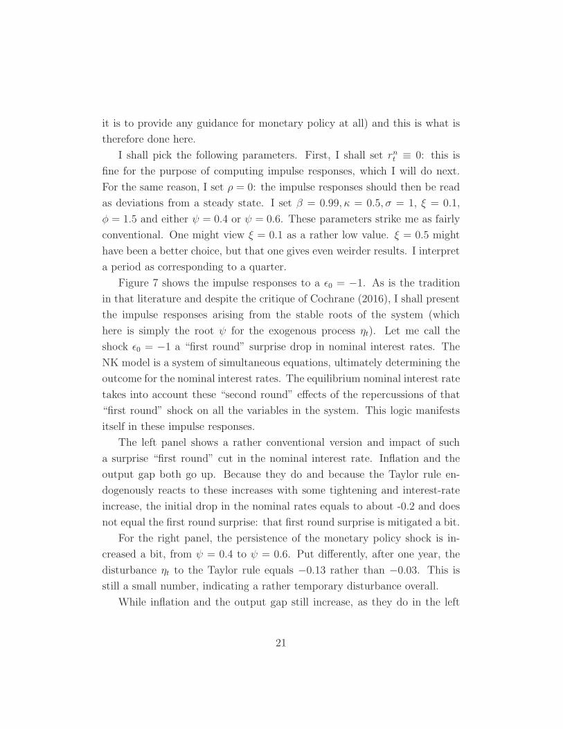
Figure 7 shows the impulse responses to a ǫ0 = −1. As is the tradition

in that literature and despite the critique of Cochrane (2016), I shall present

the impulse responses arising from the stable roots of the system (which

here is simply the root ψ for the exogenous process ηt). Let me call the

shock ǫ0 = −1 a “first round” surprise drop in nominal interest rates. The

NK model is a system of simultaneous equations, ultimately determining the

outcome for the nominal interest rates. The equilibrium nominal interest rate

takes into account these “second round” effects of the repercussions of that

“first round” shock on all the variables in the system. This logic manifests

itself in these impulse responses.

The left panel shows a rather conventional version and impact of such

a surprise “first round” cut in the nominal interest rate. Inflation and the

output gap both go up. Because they do and because the Taylor rule en-

dogenously reacts to these increases with some tightening and interest-rate

increase, the initial drop in the nominal rates equals to about -0.2 and does

not equal the first round surprise: that first round surprise is mitigated a bit.

For the right panel, the persistence of the monetary policy shock is in-

creased a bit, from ψ = 0.4 to ψ = 0.6. Put differently, after one year, the

disturbance ηt to the Taylor rule equals −0.13 rather than −0.03. This is

still a small number, indicating a rather temporary disturbance overall.

While inflation and the output gap still increase, as they do in the left

21

0 0.5 1 1.5 2time (quarters)

-0.2

0

0.2

0.4

0.6

0.8

resp

onse

Imp. resp. to mon. shock, φ=1.5, ψ=0.4

πx

i

0 0.5 1 1.5 2time (quarters)

0

0.2

0.4

0.6

0.8

resp

onse

Imp. resp. to mon. shock, φ=1.5, ψ=0.6

π

x

i

Impulse responses to ǫ0 = −1, if ψ = 0.4 Impulse responses to ǫ0 = −1, if ψ = 0.6.

Figure 7: Impulse responses in a three-equation New Keynesian Model.

panel, nominal interest rates now increases as well. The endogenous second-

round effects now more than compensate for the first-round decrease of the

nominal interest rate. Put differently, the inflation now rises so much, that

the Taylor rule endogenously forces the central bank to raise rates, in order

to combat these movements. One can imagine these dynamics to come about

from a somewhat topsy-turvy discussion in the governing council of a central

bank, running as follows: “let’s stimulate inflation and the output gap, by

cutting the interest rates and doing so with some persistence. We obviously

all understand, that we then have to tighten interest rates in order to cool

off these developments. As a results, we shall end up raising rather than

lowering rates now.” I can see how this could be confusing. It may be easier

to approach this from the outcome of the calculations right away. Following

those deliberations, the central bank president could then announce to the

eagerly waiting press, that it was decided to raise nominal interest rates and

somewhat persistently so, as it is the judgement of the council, that this will

increase inflation rates and the output gap.

There are a number of ways to react to these calculations in the right panel

and to such an announcement by a central bank president. One reaction is

22

to view them as entirely logical. Of course, there is a Fisherian effect! If the

inflation is higher, nominal interest rates need to be higher too. However,

from a conventional Keynesian analysis, the right panel does look odd: it

looks as if a somewhat persistent rise in nominal rates rather than a somewhat

persistent drop in nominal rates will stimulate the economy.

These calculations also point out, that the zero lower bound should have

hardly been a concern. In order to stimulate the economy and to move away

from the specter of deflation, all that the central banks needed to have done

post-2008 is to raise nominal interest rates with some persistence.

I do not wish to judge here, whether I trust this conclusion as a matter of

practical policy advice, though my intuition tells me to attach ample warn-

ings to it: driven though, possibly, by faulty intuition due to the influence

by that defunct academic scribbler mentioned previously. More importantly,

though, I just wish to point out that this is a straightforward implication of

the most basic, standard New Keynesian model, for an entirely reasonable

set of parameters.

One can treat this all as a “bug” of course. There are “fixes” in the

literature to address this implication, see e.g. Garin et al (2016), as well as

other “odd” implications of the benchmark New Keynesian literature, such

as the forward guidance puzzle, the reliance on Euler equations and the like.

One has to wonder, whether the direction to deviate from the simple three-

equation New Keynesian model is unique. If not, then it should be likewise

equally legitimate to treat these properties as a feature and not a bug, and be

allowed to deviate from the baseline model such as to enhance them. Which

one then is most appropriate for monetary policy advice? Why is the “bug”

perspective more appropriate than the “feature” perspective? Is it legitimate

to return to conventional Keynesian logic and intuition time and again as a

model selection device? We may risk being stuck in groundhog day forever.

This echoes the concerns more formally addressed in Gilles Saint-Paul (2018).

A summary of this neo-Fisherian challenge is this. The New Keynesian

model is “sold” as a modern version of the textbook IS-LM thinking. It works

23

quite differently, though: perhaps very differently. Consider for example, the

zero lower bound problem. The benchmark three equation model implies

that there shouldn’t be much of a zero lower bound problem, if you ever

land there by accident: just raise rates and promise to keep them above

the Taylor rule target for a little while, in order to increase inflation and

economic activity. New Keynesian theory is a lot more Neo-Fisherian than

their advocates may lead us to believe, see also Cochrane (2016). The New

Keynesian model generally appears to have several “odd” features, which

may call into question whether it is all that useful as a reliable guide for

monetary policy as its advocates have us believe.

5 Conclusions

DSGE models were meant to rise to the Lucas (1976) challenge of construct-

ing general equilibrium models with deep parameters, to be used as workhorse

models for e.g. monetary policy analysis. But challenges remain. This paper

has discussed a few of them. The central issue of the impact of monetary

policy on yield spreads and asset prices is often ignored in DSGE models

or kept essentially separate from allocations. While much progress has been

made on considering financial frictions in DSGE models, the models need to

allow more room for private markets to address these frictions, rather than

to call on economic policy for their resolution. The Phillips-curve tradeoff, so

central to thinking about monetary policy and much of the DSGE literature,

may hardly be there. New Keynesian models, which have largely become the

benchmark approach to thinking about monetary policy in central banks,

have neo-Fisherian properties. These are rarely advertised or, alternatively,

treated as “bugs” by researchers, driven by conventional thinking about how

monetary policy works, rather than an opportunity to escape the groundhog

day of repeating conventional insights. A constructive approach here might

be to apply the approach of Brinca et al (2016) and extend it to the realm

of these and other challenges to provide a guide to future research. In sum,

24

the glass is half full. Or half empty. Take your pick.

References

[1] Aiyagari, R. (1994), “Uninsured Idiosyncratic Risk and Aggregate Sav-

ing.” Quarterly Journal of Economics, vol. 109, 659-684.

[2] Bansal, Ravi and Amir Yaron (2004), “Risk for the Long Run: A Po-

tential Resolution of Asset Pricing Puzzles.” Journal of Finance, vol. 59,

no. 4, pp. 1481–1509.

[3] Barro, Robert J. (2006), “Rare Disasters and Asset Markets in the

Twentieth Century.” Quarterly Journal of Economics, vol. 121, no.3.,

pp. 823-66.

[4] Borovicka and Lars Peter Hansen (2016), “Term Structure of Uncer-

tainty in the Macroeconomy.” Chapter 20 in Handbook of Macroeco-

nomics, Vol. 2B, eds. John Taylor and Harald Uhlig, Elsevier, North

Holland, pp. 1641-1696.

[5] Brinca, P., V.V. Chari, P.J. Kehoe and E. McGrattan (2016), “Account-

ing for Business Cycles,” Chapter 13 in Handbook of Macroeconomics,

Vol. 2B, eds. John Taylor and Harald Uhlig, Elsevier, North Holland,

pp. 1013-1064.

[6] Cochrane, John H. (2016), “Do Higher Interest Rates Raise or Lower

Inflation?” Draft, Hooever Institution, Stanford.

[7] Coenen, Gnter, Christopher J. Erceg, Charles Freedman, Davide

Furceri, Michael Kumhof, Ren Lalonde, Douglas Laxton, Jesper Lind,

Annabelle Mourougane, Dirk Muir, Susanna Mursula, Carlos de Re-

sende, John Roberts, Werner Roeger, Stephen Snudden, Mathias Tra-

bandt, and Jan in’t Veld (2012), “Effects of Fiscal Stimulus in Structural

25

Models.” American Economic Journal: Macroeconomics, 4 (1), pp. 22–

68.

[8] Coeurdacier, Nicolas, Helne Rey and Pablo Winant (2011), “The Risky

Steady State,” American Economic Review vol. 101, no. 3 (May), pp.

398–401.

[9] Crump, Richard K., Stefano Eusepi and Emanuel Moench (2018), “The

Term Structure of Expectations and Bond Yields,” Federal Reserve

Bank of New York Staff Reports No. 775.

[10] de Fiore, Fiorella and Harald Uhlig (2011), “Bank Finance versus Bond

Finance.” Journal of Money, Credit and Banking (2011), Blackwell Pub-

lishing, vol. 43(7), October, pp.1399–1421.

[11] de Fiore, Fiorella and Harald Uhlig (2015), “Corporate Debt Structure

and the Financial Crisis.” Journal of Money, Credit and Banking, De-

cember, vol. 47, no. 8, pp. 1571–1598.

[12] Del Negro, Marco, Marco P. Giannoni, and Frank Schorfheide (2015),

“Inflation in the Great Recession and New Keynesian Models.” Ameri-

can Economic Journal: Macroeconomics, 7(1), pp. 168–196.

[13] Drautzburg, Thorsten and Harald Uhlig (2015), “Fiscal Stimulus and

Distortionary Taxation.” Review of Economic Dynamics, vol. 18, pp

894–920.

[14] Epstein, Larry G. and Stanley E. Zin (1989), ”Substitution, Risk Aver-

sion and the Temporal Behavior of Consumption and Asset Returns: A

Theoretical Framework.” Econometrica, pp. 937-968.

[15] Fernandez-Villaverde, J., J.F. Rubio-Ramırez and F. Schorfheide (2016),

“Solution and Estimation Methods for DSGE Models.” Chapter 9 in

Handbook of Macroeconomics, Vol. 2B, eds. John Taylor and Harald

Uhlig, Elsevier, North Holland, pp. 527–724.

26

[16] Fratto, Chiara and Harald Uhlig (2016), “Accounting for Post-Crisis

Inflation: A Retro Analysis,” draft, University of Chicago.

[17] Galı, Jordi (2008), Monetary Policy, Inflation, and the Business Cy-

cle: An Introduction to the New Keynesian Framework.) Princeton, NJ:

Prince- ton University Press.

[18] Garn, Julio, Robert Lester and Eric Sims (2016), “Raise Rates to raise

inflation? Neo-Fisherianism in the New Keynesian Model.” NBER WP

22177, April.

[19] Gertler, Mark and Peter Karadi (2011), “A model of unconventional

monetary policy.” Journal of Monetary Economy, vol. 58, pp. 17-34.

[20] Gertler, Mark and Nobuhiro Kiyotaki (2011), “Financial intermediation

and credit policy in business cycle analysis.” Chapter 11 in Handbook

of Monetary Economics, 3(A), eds. Benjamin M. Friedman and Michael

Woodford, Elsevier, North Holland, 547–599.

[21] Golosov, M., A. Tsyvinski, N. Werquin, “Recursive Contracts and En-

dogenously Incomplete Markets.” Chapter 10 in Handbook of Macroe-

conomics, Vol. 2A, eds. John Taylor and Harald Uhlig, Elsevier, North

Holland, pp. 725-841.

[22] Gertler, M., N. Kiyotaki and A. Prestipino (2016), “Wholesale Bank-

ing and Bank Runs in Macroeconomic Modeling of Financial Crises,”

Chapter 16 in Handbook of Macroeconomics, Vol. 2B, eds. John Taylor

and Harald Uhlig, Elsevier, North Holland, pp. 1345–1425.

[23] Gourio, Francois (2012), “Disaster Risk and Business Cycles.” American

Economic Review, vol. 102, no. 6 (October), pp. 34–66.

[24] Guerrieri, Veronica and Harald Uhlig (2016), “Housing and Credit Mar-

kets: Booms and Busts.” Chapter 17 in Handbook of Macroeconomics,

Vol. 2B, eds. John Taylor and Harald Uhlig, Elsevier, North Holland,

pp. 1427-1496.

27

[25] Hansen, Lars Peter and Thomas J. Sargent (2007), Robustness,Princeton

University Press, Princeton, NJ.

[26] Kaplan, Greg, Benjamin Moll and Giovanni Violante (2018), “Monetary

Policy According to HANK”. American Economic Review, vol. 108, no.

3 (March), 697–743.

[27] Keynes, John Maynard (1936), “The General Theory of Employment

Interest and Money.” Macmillan, London (reprinted 2007).

[28] Kliem, Martin and Alexander Meyer-Gohde (2018), “(Un)expected

Monetary Policy Shocks and Term Premia.” Draft, Bundesbank, Ger-

many.

[29] Krueger, Dirk and Harald Uhlig (2006), “Competitive Risk Sharing Con-

tracts with One-Sided Commitment.” Journal of Monetary Economics,

vol. 53, pp. 1661-1691.

[30] Krueger, Dirk and Harald Uhlig (2018), “Neoclassical growth with long-

term one-sided commitment contracts.” Draft, University of Chicago.

[31] Lettau, Martin and Harald Uhlig (2002), “The Sharpe Ratio and Prefer-

ences: A Parametric Approach,” Macroeconomic Dynamics, 6(2), April,

242-65.

[32] Linde, J. F. Smets and R. Wouters (2016), “Challenges for Central

Banks’ Macro Models,” Chapter 28 in Handbook of Macroeconomics,

Vol. 2B, eds. John Taylor and Harald Uhlig, Elsevier, North Holland,

pp. 2185–2262.

[33] Lucas, Robert E., Jr. (1976), “ Econometric Policy Evaluation: A Cri-

tique.” Carnegie-Rochester Conference Series on Public Policy, vol. 1.,

pp. 19–46.

[34] Lucas, Robert E., Jr. (1978), “Asset Prices in an Exchange Economy.”

Econometrica, vol. 46, no. 6, pp. . 1429-45.

28

[35] McGrattan, Ellen R. (2015), “Monetary Policy and Employment.” Eco-

nomic Policy Paper 15-7, Federal Reserve Bank of Minneapolis.

[36] Mehra, Rajnish and Edward C. Prescott (1985), “The Equity Premium:

A Puzzle.” Journal of Monetary Economics, vol. 15, no. 2, pp. 145-61.

[37] Nakamura, Emi and Jon Steinsson (2018), “ High Frequency Identica-

tion of Monetary Non-Neutrality: The Information Effect,” Quarterly

Journal of Economics, forthcoming.

[38] Piazzesi, Monika and Martin Schneider (2007), “Equilibrium Yield

Curves.’ in NBER Macroeconomics Annual 2006, Kenneth Rogoff and

Michael Woodford, eds., Cambridge MA: MIT Press, 389-442.

[39] Rudebusch, Glenn D., and Eric T. Swanson (2012), “The Bond Premium

in a DSGE Model with Long-Run Real and Nominal Risks.” American

Economix Journal: Macroeconomics, vol. 4, no. 1, pp. 105-143.

[40] Saint-Paul, Gilles (2018), “The Possibility of Ideological Bias in Struc-

tural Macroeconomic Models.” American Economic Journal: Macroeco-

nomics, vol. 10, no. 1, pp. 216-241.

[41] Schmitt-Grohe, Stephanie and Martin Uribe (2004), “Solving dynamic

general equilibirum models using a second-order approximation to the

policy function,,’ Journal of Economic Dynamics and Control, vol. 28,

pp. 755-775.

[42] Smets, Frank and Raf Wouters (2007), “ Shocks and Frictions in US

Business Cycles: A Bayesian DSGE Approach.” The American Eco-

nomic Review, vol 97, no. 3, pp. 586–606.

[43] Tallarini, Thomas D. (2000), “Risk-sensitive real business cycles.” Jour-

nal of Monetary Economics, vol. 45, no. 3, pp. 507-532.

[44] Uhlig, Harald (1999), “A toolkit for analysing nonlinear dynamic

stochastic models easily,” in Ramon Marimon and Andrew Scott, eds,

29

Computational Methods for the Study of Dynamic Economies, Oxford

University Press, Oxford, pp. 30-61.

[45] Uhlig, Harald (2005), “What are the effects of monetary policy on out-

put? Results from an agnostic identification procedure.” Journal of

Monetary Economics, vol. 52, pp. 381-419.

[46] Uhlig, Harald (2007), “Explaining Asset Prices with External Habits

and Wage Rigidities in a DSGE Model.” American Economic Review,

Papers and Proceedings, vol. 97, no 2 (May), pp. 239-243.

[47] Uhlig, Harald (2012), “Economics and Reality.” Journal of Macroeco-

nomics vol. 34, pp. 29-41.

[48] Uhlig, Harald (2018), “Easy EZ for DSGE,” draft, University of Chicago.

[49] Ulrich, Maxim (2015), “Inflation Ambiguity and the Term Structure of

U.S. Government Bonds.” Draft, Columbia Business School.

[50] van Binsbergen, Jules H., Jesus Fernandez-Villaverde, Ralph S.J. Koi-

jen, and Juan Rubio-Ramirez (2012), “The term structure of interest

rates in a DSGE model with recursive preferences,” Journal of Mone-

tary Economics, 59(7), pp. 634-648.

[51] Weitzman, Martin L. (2007), “Subjective Expectations and Asset-

Return Puzzles.” American Economic Review, vol. 97, no. 4, pp 1102-

1130.

[52] Wieland, V., E. Afanasyeva, M. Kuete, J. Yoo (2016), “New Methods for

Macro-Financial Model Comparison and Policy Analysis,” Chapter 15

in Handbook of Macroeconomics, Vol. 2A, eds. John Taylor and Harald

Uhlig, Elsevier, North Holland, pp. 1241-1319.

[53] Zhao, Guihai (2018), “Ambiguity, Nominal Bond Yields, and Real Bond

Yields.’ draft, Bank of Canada.

30