UHF Radiometry for Ice Sheet Subsurface Temperature Sensing

K. C. JezekJoel T. Johnson, L. Tsang, C. C. Chen, M. Durand, G. Macelloni,

M. Brogioni, Mark Drinkwater, Ludovic Brucker

M. Aksoy, M. Andrews, D. Belgiovane, A. Bringer, Y. Duan, H. Li, S. Tan, T. Wang, C. Yardim

Motivation

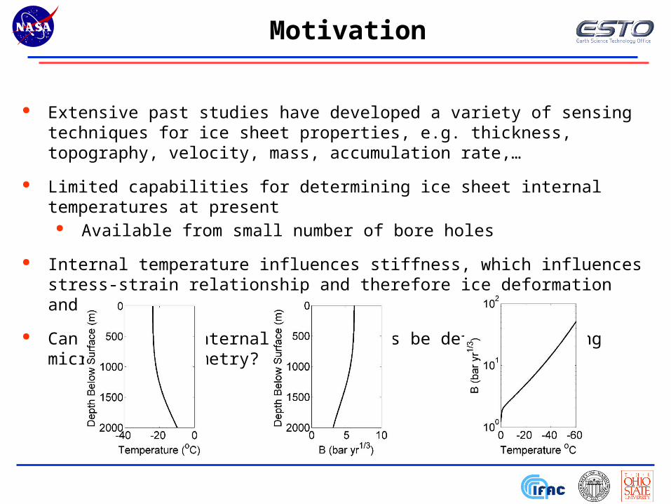
Extensive past studies have developed a variety of sensing techniques for ice sheet properties, e.g. thickness, topography, velocity, mass, accumulation rate,…

Limited capabilities for determining ice sheet internal temperatures at present Available from small number of bore holes

Internal temperature influences stiffness, which influences stress-strain relationship and therefore ice deformation and motion

Can ice sheet internal temperatures be determined using microwave radiometry?

UWBRAD Science Goals

• Ice sheet temperature at 10 m depth, 1 K accuracy– 10 m temperatures approximate the mean annual temperature, an

important climate parameter

• Depth-averaged temperature from 200 m to 4 km (max) ice sheet thickness, 1 K accuracy

– Spatial variations in average temperature can be used as a proxy for improving temperature dependent ice-flow models

• Temperature profile at 100 m depth intervals, 1 K accuracy – Remote sensing measurements of temperature-depth profiles

can substantially improve ice flow models

• Measurements all at minimum 10 km resolution– Time stamped and geolocated by latitude and longitude

Design an instrument that can measure:

Emission Physics

• In absence of scattering, thermal emission from ice sheet could be treated as a 0th order radiative transfer process

• Similar to emission from the atmosphere: temperature profiling possible if strong variations in extinction with frequency (i.e. absorption line resonance)

• Ice sheet has no absorption line but extinction does vary with frequency– Motivates investigating brightness temperatures as function of frequency

• Inhomogeneities causing scattering or other layering effects are additional complication

• First step is to demonstrate plausibility using models

Zeroth Order Tb Model

• Zeroth order models used to illustrate basic processes• Robin model of ice sheet internal temperatures is

(assumes homogeneous ice driven by geothermal heat flux, no lateral advection• In absence of scattering, thermal emission from ice sheet could be treated as

a 0th order radiative transfer process

• Similar to emission from the atmosphere: temperature profiling possible if strong variations in extinction with frequency (i.e. absorption line resonance)

• Ice sheet has no absorption line but extinction does vary with frequency– Motivates investigating brightness temperatures as function of frequency

5

500 MHz Model results suggest Tb Sensitivity at Depth and Depend on presence of subglacial water

Jezek and others, 2015

UHF Behavior for Antarctic Parameters

Evidence from SMOS

1

SMOS data over Lake Vostok (East Antarctic Plateau)

55° 25°

The analysis of SMOS data point out a relationship between Tb and Ice Thickness

Brogioni, Macelloni, Montomoli, and Jezek, 2015

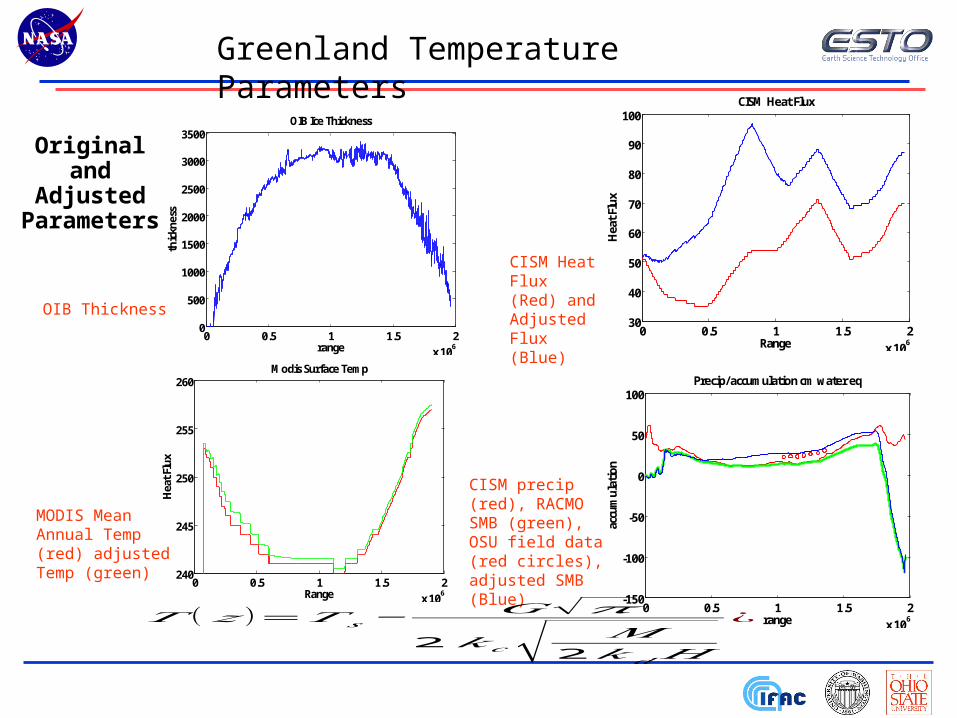
Original and Adjusted

Parameters

0 0.5 1 1.5 2x 106

-150

-100

-50

0

50

100Precip/accumulation cm water eq

rangeac

cum

ulati

on

0 0.5 1 1.5 2x 106

0

500

1000

1500

2000

2500

3000

3500OIB Ice Thickness

range

thic

knes

s

0 0.5 1 1.5 2x 106

30

40

50

60

70

80

90

100CISM Heat Flux

Range

Hea

t Flu

x

0 0.5 1 1.5 2x 106

240

245

250

255

260Modis Surface Temp

Range

Hea

t Flu

x

CISM Heat Flux (Red) and Adjusted Flux (Blue)

CISM precip (red), RACMO SMB (green), OSU field data (red circles), adjusted SMB (Blue)

MODIS Mean Annual Temp (red) adjusted Temp (green)

OIB Thickness

𝑇 (𝑧 )=𝑇 𝑠−𝐺√𝜋

2𝑘𝑐 √ 𝑀2𝑘𝑑𝐻

¿

Greenland Temperature Parameters

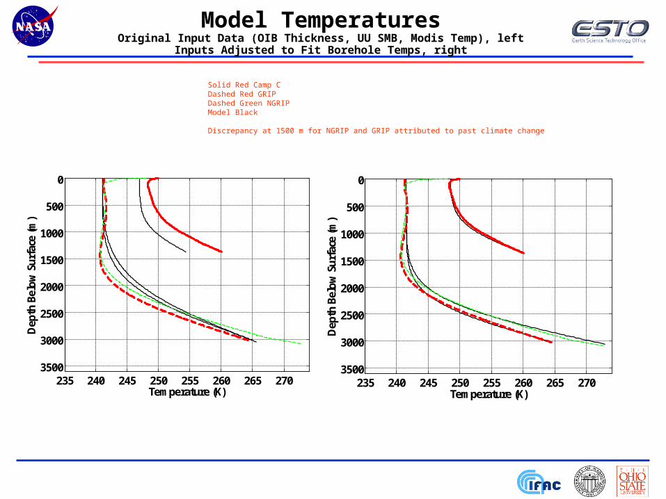
Model TemperaturesOriginal Input Data (OIB Thickness, UU SMB, Modis Temp), left

Inputs Adjusted to Fit Borehole Temps, right

235 240 245 250 255 260 265 270

0

500

1000

1500

2000

2500

3000

3500

Temperature (K)

Dep

th B

elow

Sur

face

(m)

235 240 245 250 255 260 265 270

0

500

1000

1500

2000

2500

3000

3500

Temperature (K)

Dep

th B

elow

Sur

face

(m)

Solid Red Camp CDashed Red GRIPDashed Green NGRIPModel Black

Discrepancy at 1500 m for NGRIP and GRIP attributed to past climate change

Greenland Brightness Temperatures Cloud Model, SMOS, SMAP

• Cloud model Tb estimate based on

temperature profiles derived from

OIB thickness, CISM heat flux,

RACMO SMB, MODIS surface

temp. Parameter then corrected to

match CC, NGRIP, GRIP temps.

• 1.4 GHz data forced to align with

SMOS data (black) using a constant

multiplier. Same multiplier applied

to other frequencies.

• Variations are small at 1.4 GHz along

flight path because temperature

profiles are more uniform in depth.

500 MHz anomaly associated with

region of assigned basal melt

240 250 260 270 280

0

500

1000

1500

2000

2500

3000

3500

Temperature (K)

Dep

th B

elow

Sur

face

(m)

0

0.5

1

1.5

2

x 109

0 0.5 1 1.5 2x 106

Range

Spectrum Waterfall

Rang

e

225

230

235

240

0.5 GHz B Model1.0 R “”1.4 C “”2.0 G “”SMOS Bla (thick) (Jan. 2014)SMAP B (thick) (April, 2015)

Oswald and Gogineni, Subsurface Water Map

Fre

qu

ency

DMRT-ML Model - Antarctica

• DMRT-ML model (Picard et al, 2012) widely used to model emission from ice sheets (Brucker et al, 2011a) and snowpacks (Brucker et al, 2011b)

– Uses QCA/Percus-Yevick pair distribution for sticky or non-sticky spheres– RT equation solved using discrete ordinate method– Need layer thickness, temperature, density, and grain size for multiple layers – Recommended grain size is 3 X in-situ measured grain sizes

• DMRT-ML computed results for DOME-C density/grain size profiles vs. frequency

Lower frequencies“see” warmer iceat greater depths

TB varieswith internalT(z)

Aksoy and others, 2014)

Additional Factors

• Include statistical model of density with depth (Gaussian variability with a defined correlation length)

• Capture layering effects using coherent and partially coherent radiative transfer models

• Include interface roughness• Include layer conductivity at depth

0 50 100200

210

220

230

2 GHz Tb: ice sheetwith upper low density strata

.1 m layer thickness

Total Strata Thickness (m)

Tb

Figure 7. Brightness temperature for changing the total thickness of the near surface low density layer. The discrete layer thickness is constant at 0.1 m. Variability is a consequence of recomputing the density function for each calculation. The red curve shows only the effect so the subsurface layers. The blue cure includes the loss at the air snow interface.

0.2 0.4 0.6 0.8 1

0

20

40

60

80

100

Combined Drinkwater and random density

Density (gm/cc)

Dep

th (m

)

Greenland Brightness Temp vs. Frequency

• Antarctic geophysical cases: low accumulation rates result in temp profiles that increase with depth

• Strong changes in TB vs. frequency

• Higher accumulation rates in Greenland (at least for GISP site) result in more uniform temp profile vs. depth

• Smaller changes in TB vs. frequency

• Need instrumentthat can capturethese variations

0 1000 2000 3000

150

200

250

Tb(

K)

frequency(Hz)

1585 Simulated Tb vs Freq profiles

Antarctica

Greenland(GISP) Greenland

(GISP)

Blue: With AntennaRed: Without Antenna

Blue: Simulated ProfilesRed: GISP Data

Forward Model Assessment

• Used “Dome-C”-type physical parameters– Including density fluctuations with correlation length parameter

• Results show:– Coherent effects can be significant if density correlation length <<

wavelength; otherwise good agreement between models

0.5 1 1.5 2150

200

250l = 3cm

Brig

htne

ss T

empe

ratu

re (

K)

0.5 1 1.5 2150

200

250l = 5cm

0.5 1 1.5 2200

220

240

260l = 10cm

frequency (GHz)Brig

htne

ss T

empe

ratu

re (

K)

0.5 1 1.5 2200

220

240

260l = 40cm

frequency (GHz)

Cloud

DMRT/MEMLS

Coherent

Tan and others, 2015)

Greenland Retrieval Studies

• Generated simulated 0.5-2 GHz observations of “GISP-like” ice sheets for varying physical properties (500 “truth” cases)

– Including averaging over density fluctuations• For each truth case, generate 100 simulated retrievals with expected noise

levels (i.e. ~ 1 K measurement noise per ~ 100 MHz bandwidth)• Select profile “closest” to simulated data as the retrieved profile, and

examine temperature retrieval error

• Errors in this simulation meet science requirements• Additional simulations continuing over Greenland flight path

Ultra-wideband software defined radiometer (UWBRAD)

• UWBRAD=a radiometer operating 0.5 – 2 GHz for internal ice sheet temperature sensing

• Requires operating in unprotected bands, so interference a major concern

• Address by sampling entire bandwidth ( in 100 MHz channels) and implement real-time detection/mitigation/use of unoccupied spectrum

• Supported under NASA 2013 Instrument Incubator Program

Frequency Channels 0.5-2 GHz, 15 x 100 MHz channels Polarization Single (Right-hand circular)

Observation angle Nadir Spatial Resolution 1 km x 1 km (1 km platform altitude) Integration time 100 msec Ant Gain (dB) /Beamwidth

11 dB 30

Calibration (Internal) Reference load and Noise diode sources Calibration (External) Sky and Ocean Measurements

Noise equiv dT 0.4 K in 100 msec (each 100 MHz channel) Interference Management

Full sampling of 100 MHz bandwidth in 16 bits resolution in each channel; real time “software

defined” RFI detection and mitigation Initial Data Rate 700 Megabytes per second (10% duty cycle)

Data Rate to Disk <1 Megabyte per second

Hybrid Front End Design (13 channels)

Radiometers require frequent calibration against hot and cold reference loads

Many radiometers use a Dicke switch to alternate connection to the load and the antenna

UWBRAD radiometer is controlled by hybrid couplers and a 0-180 degree selectable phase shifter providing rapid comparison between the load and the signal.

This hybrid scheme improves the system noise figure without having to resort to physically large ferrite cores to blank transient signals from a switch.

Front End Design Parameters Review of radiometer frequency plan completed

– Based on RFI considerations, 15 adjacent channel frequency plan revised to 13 separated channels in 2nd Nyquist of ADC

Trade study of alternate radiometer front end design based on Dicke Switch architecture also completed

Baseline “hybrid” radiometer design updated to include RF filtering Build of “Hybrid radiometer” LNA/hybrid block in progress to assess

performance

Digital Subsystem

• Digital Subsystem based around the ATS9625 card from AlazarTech, Inc.– 2 channel, 250 MSPS,16 bit/sample data acquisition card– Achieves high throughput to host PC– Team has past experience with similar AlazarTech

board and software interface– RFI processing to be performed on host PC

• Each board can handle 2 100 MHz channels

• 7 boards used for 13 channels

• One host PC can accommodate 2 ATS9625 boards– Need 4 PC’s

• 2 boards and host PC have been acquired and are being used for code development and throughput studies

Antenna Design

0.5 0.6 0.7 0.8 0.9 1 1.1 1.2 1.3 1.4 1.5 1.6 1.7 1.8 1.9 250

52

54

56

58

60

62

64

66

68

70

Frequency [GHz]

Bea

mw

idth

[d

egre

es]

H = 37”

Diameter: 10 inches

Diameter: 1.1 inches

Cone Angle = 13.2°

56 Turns

Antarctic and Greenland Field Deployments

• April or October 2016 Greenland Airborne Campaign

• Continued discussions with Ken Borek Air, Ltd. for use of Bassler aircraft

• Budget for 5 days/ 40 flight hours consistent with project plan

• IFAC will deploy an L-band radiometer at DOME-C November 2015-January 2016 (30-45 day campaign)

• Plan to include UWBRAD tower deployment at DOME-C as part of the IFAC Project

• Would be desirable to include full 13 channel system, but a 4 channel system could provide valuable information

• Developing plan to deploy UWBRAD 4 channel system at DOME-C

• Likely will be supported by IFAC personnel only; project team will train IFAC personnelAntenna

UWBRAD Enclosure

Status Summary

• Project progressing according to schedule

• No major risks identified

• Goals for next 6 months:

– Four channel unit finished, tested, and underway to Antarctica

– Thirteen channel unit build underway

– Differing TB profiles versus frequency in Greenland will continue to be focus of retrieval analyses

• Finish observation simulation study for Greenland flight path

– RFI processing algorithms will be focus of software development

– Design of “backup” Dicke switching architecture will continue

• No major impact on development schedule since majority of front end design is common to two approaches

Conclusions

• Multi-frequency brightness temperature measurements can provide additional information on internal ice sheet properties

– Increased penetration depth in pure ice and reduced effect of scatterers as frequency decreases

• SMOS measurements show evidence of subsurface temperature contributions to observed 1.4 GHz measurements

• UWBRAD proposed to allow further investigations– Website at: http://research.bpcrc.osu.edu/rsl/UWBRAD/

• UWBRAD began April 2014, goal for airborne deployment in 2016 to demonstrate performance