ucge reports - university of calgary · ucge reports number 20269 ... carina butterworth ... thanks...
TRANSCRIPT
UCGE Reports
Number 20269
Department of Geomatics Engineering
Measuring Seasonal Permafrost Deformation with Differential Interferometric Synthetic Apertur e
Radar (URL: http://www.geomatics.ucalgary.ca/research/publications/GradTheses.html)
by
Carina Butterworth
April 2008
UNIVERSITY OF CALGARY
Measuring Seasonal Permafrost Deformation with Differential Interferometric
Synthetic Aperture Radar
by
Carina Butterworth
A THESIS
SUBMITTED TO THE FACULTY OF GRADUATE STUDIES
IN PARTIAL FULFILLMENT OF THE REQUIREMENTS FOR THE
DEGREE OF MASTER OF SCIENCE
DEPARTMENT OF GEOMATICS ENGINEERING
CALGARY, ALBERTA
APRIL, 2008
© Carina Butterworth 2008
iii
ABSTRACT
Permafrost has been shown as a potential indicator of climate change. Because of the
vast area permafrost covers and the remoteness of these areas, a cost effective, remote
system is required to monitor small annual changes. Differential Interferometric
Synthetic Aperture Radar (DInSAR) has been proposed as a possible tool to monitor
small height changes of the surface of the permafrost active layer. Four sets of DInSAR
images were processed using three-pass interferometric methods and were factorized into
the possible decorrelation components. These components include incidence angles,
Doppler centroid differences, ionospheric activity, and coherence. The resulting
displacement maps were compared structurally to conventionally surveyed ground truth
data and the magnitude was compared with results of a permafrost heave model. One of
the four sets of data was found to correspond to the ground truth data and the permafrost
heave model. This data set had a high signal to noise ratio (SNR) and low Doppler
centroid difference at an incidence angle of 38o. The other sets of data failed to create a
reliable differential interferogram. The author concluded that DInSAR shows strong
potential as a tool to map permafrost displacement, but further research is required.

iv
ACKNOWLEDGEMENTS
I wish to express my sincere gratitude to my supervisor, Dr. Matthew Tait, for all his
encouragement and support throughout the course of my graduate studies. I would also
like to acknowledge his help in providing me with the required images and surveyed
ground data for the processing and validation of my work.
Thank you to Dr. Michael Collins for accepting me as his student upon the leave of Dr.
Tait from the University of Calgary and his advice for completing my thesis.
Davor Gugolj had completed the work on the permafrost heave model and allowed me to
use the results for the purposes of validating this thesis work.
Thanks to Dr. Brian Moorman for his advice on interpreting the errors in the images.
Sincere thanks to my dad, Kevin Dunn, for his long hours of assistance in editing.
Financial support came from the University of Calgary in the form of Graduate Research
Scholarships, Institute of Sustainable Energy, Environment and Economy, teaching and
research assistantships, and personal funding from Dr. Tait. Other financial support came
in the form of scholarships from the Graduate Student’s Association, Association of
Professional Engineers, Geologists and Geophysicists of Alberta (APEGGA), Alberta
Heritage Fund, and Alberta Land Surveyor’s Association (ALSA). All these are
gratefully acknowledged.
v
To my wonderful, supportive husband, Anthony And our exceptional son, Karl

vi
TABLE OF CONTENTS
ABSTRACT....................................................................................................................... iii
ACKNOWLEDGEMENTS............................................................................................... iv
TABLE OF CONTENTS................................................................................................... vi
LIST OF TABLES.............................................................................................................. x
LISTS OF FIGURES ......................................................................................................... xi
NOTATION..................................................................................................................... xiii
1.0 INTRODUCTION ...................................................................................................1
2.0 BACKGROUND .....................................................................................................2
2.1 Permafrost ....................................................................................................2
2.2 Climate Change............................................................................................4
2.3 Historical Permafrost Monitoring................................................................6
2.3.1 Traditional Differential Precise Leveling ........................................7
2.3.2 Probing.............................................................................................9
2.3.3 Frost / Thaw Tubes ........................................................................10
2.3.4 Ground Penetrating Radar..............................................................12
2.3.5 Electrical Resistivity Imaging........................................................13
2.3.6 Circumpolar Active Layer Monitoring ..........................................14
2.3.7 Carrier Phase Differential Global Positioning System ..................14
2.4 Differential Interferometric Synthetic Aperture Radar..............................16
2.5 Problem Statement .....................................................................................17
3.0 SYNTHETIC APERTURE RADAR INTERFEROMETRY................................18
3.1 Introduction................................................................................................18
3.2 The Radar Equation ...................................................................................21
3.2.1 Monostatic Point Scatterer Radar Equation...................................21
vii
3.2.2 Normalized Radar Equation...........................................................22
3.2.3 Scattering Properties ......................................................................23
3.3 Image Geometry.........................................................................................24
3.2.1 Baseline Geometry.........................................................................26
3.4 Temporal Decorrelation .............................................................................30
3.4.1 Ionospheric Activity.......................................................................31
3.4.2 Example of Atmospheric Disturbances .........................................32
3.5 Signal to Noise Ratio (SNR)......................................................................33
3.6 Doppler Centroid Differences....................................................................34
3.7 Processing Methodology............................................................................35
3.7.1 Geometric misregistration..............................................................36
4.0 COHERENCE AND PHASE UNWRAPPING ....................................................38
4.1 Coherence ..................................................................................................38
4.1.1 Imaging Geometry .........................................................................39
4.1.2 Doppler Centroid Differences and Noise.......................................41
4.1.3 Temporal and Volume Decorrelation ............................................42
4.1.4 Coherence Estimation ....................................................................43
4.2 Phase Unwrapping .....................................................................................43
5.0 DIFFERENTIAL INTERFEROMETRIC SYNTHETIC APERTURE RADAR .46
5.1 DInSAR Background .................................................................................46
5.1.1 DInSAR Geometry.........................................................................46
5.1.2 Differential Interferogram Computations ......................................48
5.1.2.1 Two-Pass Differential Interferometry................................48
5.1.2.2 Three-Pass Differential Interferometry..............................48
5.1.2.3 Four-Pass Differential Interferometry................................49
5.2 Objectives ..................................................................................................50
viii
6.0 EXPERIMENTAL DESIGN .................................................................................51
6.1 Data Background .......................................................................................51
6.1.1 Area of Interest ..............................................................................51
6.1.2 Images ............................................................................................52
6.2 SAR Processing .........................................................................................54
6.2.1 Image Registration .........................................................................54
6.2.2 Interferogram Generation...............................................................58
6.2.3 Coherence Estimation ....................................................................59
6.2.4 Phase Unwrapping .........................................................................60
6.2.5 Differential SAR Interferometry....................................................62
6.2.5.1 ENVISAT ASAR Differential Interferometry...................63
6.2.5.2 RADARSAT Differential Interferometry..........................63
6.2.6 Georeferencing...............................................................................65
6.3 Ground Data...............................................................................................65
6.3.1 Conventional Leveling...................................................................65
6.3.2 Permafrost Heave Model ...............................................................67
6.3.2.1 Thermal Regime Model .....................................................67
6.3.2.2 Snow Distribution Model...................................................68
6.3.2.3 Heave and Subsidence Model............................................68
7.0 RESULTS AND ANALYSIS................................................................................70
7.1 Data Input...................................................................................................70
7.2 Image Registration .....................................................................................73
7.3 Interferogram Generation...........................................................................74
7.4 Coherence Estimation ................................................................................75
7.5 Phase Unwrapping .....................................................................................84
7.6 Differential Interferometry.........................................................................87
7.7 Ground Data Correlation............................................................................95

ix
8.0 CONCLUSIONS AND RECOMMENDATIONS ................................................98
8.1 Conclusions................................................................................................98
8.2 Recommendations....................................................................................101
REFERENCES ................................................................................................................103

x
LIST OF TABLES
6.1 Data Set Organization ................................................................................................53
7.1 Raw data characteristics of images ............................................................................71
7.2 Incidence angles and Doppler polynomials ...............................................................72
7.3 Range and Azimuth Offsets of Image Pairs...............................................................73
7.4 Signal to Noise Ratio Statistics..................................................................................74
7.5 Baselines and their breakdown ..................................................................................75
7.6 Coherence Statistics For Set 1 ...................................................................................77
7.7 Coherence Statistics for Set 2 ....................................................................................79
7.8 Coherence Statistics for Set 3 ....................................................................................81
7.9 Coherence Statistics for RADARSAT.......................................................................83
7.10 Ionospheric activity recorded in Yellowknife............................................................85
7.11 RADARSAT Signal to Noise Ratio Statistics ...........................................................92
7.12 RADARSAT Baseline ...............................................................................................93

xi
LIST OF FIGURES
2.1 Differences in the types of permafrost and the depths.............................................2
2.2 Northern Hemisphere permafrost coverage.............................................................3
2.3 Decreasing Permafrost Regions in the North...........................................................5
2.4 Example of conventional leveling with a precise rod (a) and level (b) ...................8
2.5 Example of a permafrost Probe Rod........................................................................9
2.6 Example of a Frost / Thaw Tube............................................................................11
2.7 Water Absorption of Radiowaves..........................................................................13
2.8 Double Differencing GPS......................................................................................15
3.1 Diagram for the monostatic radar equation ...........................................................22
3.2 Backscatter power of a group of scatterers in a pixel with dominant scatterers....24
3.3 Image acquisition geometry for a single pixel.......................................................25
3.4 Baseline geometry..................................................................................................27
4.1 Example of pixel coherence...................................................................................39
5.1 Differential interferometry geometry.....................................................................47
6.1 Picture depicting the landscape and vegetation of the test area.............................51
6.2 a) Map of the area where the star represents the area of ground truth data and the
rectangle is the area of image b; b) Intensity image of the same area where the
white square represents the ground truth data area................................................52
6.3 Flow chart of DInSAR processing used to determine land deformation ...............55
6.4 June conventional leveling data collection points .................................................66
6.5 Permafrost heave model predicted elevation changes for 2005.............................69
7.1 a) 17259 & 17760 (June-July) coherence; b) 17760 & 18261 (July-August)
coherence ...............................................................................................................76
7.2 a) 17337 & 17838 (June-July) coherence; b) 17838 & 18339 (July-August)
coherence ...............................................................................................................78
7.3 a) 17302 & 17803 (June-July) coherence; b) 17803 & 18304 (July-August)
coherence ...............................................................................................................80

xii
7.4 a) June / August coherency map; b) August / September coherency map.............82
7.5 a) June / August unwrapped interferogram; b) August / September unwrapped
interferogram..........................................................................................................86
7.6 a) Set 1 unwrapped differential interferogram; b) Set 3 unwrapped differential
interferogram..........................................................................................................88
7.7 Enhanced image of set 1 differential interferogram ..............................................89
7.8 a) Set 1 displacement map; b) Set 3 displacement map.........................................90
7.9 Colour map used to visualize displacement...........................................................91
7.10 Unwrapped differential interferogram...................................................................93
7.11 RADARSAT displacement map............................................................................93
7.12 Displacement map of set 1 where blue shows zero subsidence and brown shows 6
cm of subsidence and an enlargement of the area of interest ................................95
7.13 Differential interferogram of the area of interest with flow accumulation map
overlaid ..................................................................................................................96
7.14 Displacement map compared with the permafrost heave model ...........................97

xiii
NOTATION Symbols
A differential design matrix including atmospheric parameters
Aa area of antenna related to gain
α orientation angle
A i and Bi coefficients
b baseline direction
B total baseline
BA Bandwidth in azimuth direction
Bp perpendicular baseline
BT transmitted signal bandwidth
B orthogonal baseline projection
Bcrit Critical baseline (m)
Br Data rate (kb/s)
Bdef Deformation pair baseline
Btopo Topographic pair baseline
b function of the image spectral filter
β beamwidth
c speed of light
γtotal total coherence
γgeom imaging geometry
γfdc Doppler centroid difference
γprocess processing methodology
γthermal thermal noise
γvolume volume of scatterer
γtemporal temporal decorrelation
Dp displacement of the point
xiv
DCf∆ Doppler centroid frequency
ζ Reflected angle (rad)
Fn receiver noise figure
θ look angle
θi incidence angle
G gain
Hp height of the point
h local vertical at the target point
i iteration count
I irradiance
K Boltzmann’s constant
Ls system losses
λ wavelength
|m| magnitude of the motion vector
n signal’s phase shift
n unit look vector
Pave average transmitted power
Pr power received
Pt power transmitted
pφ reference phase
Ω baseline scaling factor
R slant range
)(iRxy correlation of two pixels
ro complex amplitude of the reference image beam
r(x,y) master image signal value
S(ξo,γo) Fourier filter plane
T temperature of receiver
σ scattering cross-section

xv
σo differential scattering coefficient
V platform velocity
V visibility of the fringes
vres effective velocity of the sensor
v velocity variation
Wf filter size
φ D phase change
x pixel in azimuth direction
y pixel in range direction
* complex conjugate
<> ensemble average

xvi
Acronyms
ASAR Advanced Synthetic Aperture Radar
CALM Circumpolar Active Layer Monitoring Network
DEM Digital Elevation Model
DGPS Differential Global Positioning System
DInSAR Differential Interferometric Synthetic Aperture Radar
DORIS Doppler Orbitography and Radiopositioning Integration by Satellite
ENVISAT European Space Agency Environmental Satellite
ERS Earth Remote Sensing Satellite
ESRI Environmental Systems Research Institute
FV Fringe Visibility
GCM General Circulation Model
GIS Geographic Information System
GPR Ground Penetrating Radar
GPS Global Positioning System
ICC Intensity Cross-Correlation
InSAR Synthetic Aperture Radar Interferometry
PCV Phase Center Variation
PVC Polyvinyl Chloride
RADAR Radio Detection and Ranging
RADARSAT Radio Detection and Ranging Satellite
SAR Synthetic Aperture Radar
SLC single look complex
SNR Signal to Noise Ratio
WGS World Geodetic System
1
CHAPTER 1
INTRODUCTION
Climate change has been a topic of interest for many researchers. One of the indicators of
interest concerns the response of the permafrost active layer to increasing global
temperature. Some of the characteristics of permafrost thaw that have been considered
include the magnitude, depth, and rate of the thaw. One measure of these characteristics
is relative changes in ground surface elevation. These three characteristics have been
evaluated using this measure by means of point-based, conventional methods in places
such as Fairbanks, Inuvik, and Saluit. Because of the high cost of these conventional
methods, it was important to find a new method to monitor areas as vast as the arctic.
Satellite-based Differential Interferometric Synthetic Aperture Radar (DInSAR) is an
active microwave system that can estimate small height variations, considering that the
acquired images maintain a high coherence between each other. Unfortunately, because
the surface characteristics in the arctic tend to change rapidly during the summer
(generally June to August), synthetic aperture radar (SAR) research has not been
effective to date because of temporal decorrelation in repeat-pass observations.
Four sets of data were used in this study. The results were analyzed by factoring the
different characteristics used in processing the data and the factors affecting temporal
decorrelation. One set provided a possible displacement map solution, showing
subsidence of up to 6 cm. This map was cropped to a test area of 1 km2, where ground
measurements were acquired. When the ground data and the displacement map were
correlated in both structure and amplitude, the results appeared promising.

2
CHAPTER 2
BACKGROUND
2.1 Permafrost
As concerns about climate change continue to increase and research in the polar regions
is becoming more prominent, permafrost monitoring has become an important topic.
Permafrost has been defined as ground that remains at or below 0oC for at least two
consecutive years (Harris et al., 2003). The top soil layer, called the active layer, is the
medium that interacts with the atmosphere, causing seasonal freezing and thawing, and
therefore varying its thickness over time, distance, and area, as seen in Figure 2.1. Even
in apparent homogenous areas, the depth and extent of the freezing and thawing are
variable (Nelson et al., 1998a; Nelson et al., 1999; Miller et al., 1998) and are caused by
features such as soil texture, soil moisture, and surface vegetation (Hinkel et al., 2001a).
These features can also provide a historical record of surface temperature variations
(Guglielmin & Dramis, 1999; Nelson et al., 1998b; Nixon & Taylor, 1998; Burgess et al.,
2000; Mauro, 2004; Lachenbruch & Marshall, 1986; Beltrami & Taylor, 1994), allowing
the study of ongoing trends.
Figure 2.1: Differences in the types and depths of permafrost (Canadian Geographic, 2008)
3
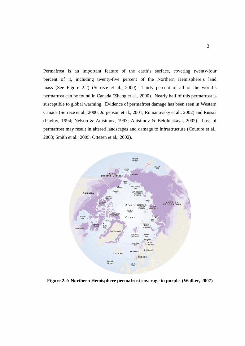
Permafrost is an important feature of the earth’s surface, covering twenty-four
percent of it, including twenty-five percent of the Northern Hemisphere’s land
mass (See Figure 2.2) (Serreze et al., 2000). Thirty percent of all of the world’s
permafrost can be found in Canada (Zhang et al., 2000). Nearly half of this permafrost is
susceptible to global warming. Evidence of permafrost damage has been seen in Western
Canada (Serreze et al., 2000; Jorgenson et al., 2001; Romanovsky et al., 2002) and Russia
(Pavlov, 1994; Nelson & Anisimov, 1993; Anisimov & Belolutskaya, 2002). Loss of
permafrost may result in altered landscapes and damage to infrastructure (Couture et al.,
2003; Smith et al., 2005; Ottesen et al., 2002).
Figure 2.2: Northern Hemisphere permafrost coverage in purple (Walker, 2007)
4
Permafrost variations are important because they potentially indicate climate change
(Harris et al., 2003). Monitoring will provide information about the relationship between
climate change and permafrost (Davis, 2001; Ishikawa, 2003). Possible characteristics of
permafrost that could provide an indication are the timing and rate of the freeze/thaw
cycle, the extent of the active layer (Nelson et al., 1993), and the deepening and
increasing failure of the active layer (Maxwell, 1997).
There are two major landforms that have been discussed in the literature with respect to
permafrost: mountainous regions (Haeberli et al., 1993; Salzmann et al., 2007) and arctic
regions (ie. plateaus, deltas, peatlands, etc.) (Laberge & Payette, 1995; Butterworth &
Tait, 2007; Nelson et al., 2002). In this study, arctic plateaus and deltas were of specific
interest because the effect of climate warming is expected to be greatest in high latitudes
(Flato et al., 2000) and approximately 14% of the northern landscape consists of arctic
plateaus or deltas. The Mackenzie Delta region was chosen because of the additional
interest in oil and gas extraction, which may cause the landscape to subside (Tait &
Moorman, 2003).
2.2 Climate Change
Climate change is a complex issue as short term fluctuations have been reported in the
past (Osterkamp et al., 1994). Notably, a century-long cyclic change was noted in the
1940s, but following that, a natural global cooling trend stopped and an abnormal
warming trend began (Gruza & Rankova, 1980). Increased snow precipitation from 1957
to 2004 and increased annual temperatures from the mid-90s were observed and are
believed to be the main drivers for accelerating permafrost thawing (Payette et al., 2004).
New temporal changes of the permafrost layer in North America have already been
reported (Allard & Rousseau, 1999; Dionne, 1978; Laprise & Payette, 1988; Laberge &
Payette, 1995; Thie, 1974). Mackay et al. (1979), Humium (2006), and Brown et al.

5
(2000) have shown that regions covered by permafrost, such as the Mackenzie Valley and
Delta, have been reduced. Figure 2.3 shows the extent of permafrost areas between 1980
and 1999 and the predicted decrease in permafrost by the year 2080.
Figure 2.3: Decreasing Permafrost Regions in the North
(National Center for Atmospheric Research, 2005)
There have been recent attempts to model the predicted changes of permafrost due to
climate change. Nelson et al. (2002) used a general circulation model (GCM) and
permafrost maps to determine the highest danger zones affected by increasing active
layer thickness. It was found that the southern limit of arctic permafrost could move 250-
350 km north by 2010 (Barsch, 1993). Using climatic, soil, and permafrost interaction
data, it was also found that the Canadian southern limit of the permafrost would move
100-200 km north as atmospheric carbon dioxide concentrations double (French, 1996)
and that 10 to 17% of the arctic permafrost would be reduced as the active layer would

6
become 10 to 50% deeper by 2050 (Anisimov & Poliakov, 2003; Janke, 2005).
Correlation of air temperatures and permafrost layers has also been used to model
permafrost subsidence. In doing so, this method found that there is a strong correlation
between ground temperatures and air temperatures (Kakunov, 1999; Oberman &
Mazhitova, 2001).
Permafrost soil contains approximately 30% of the world’s soil carbon dioxide and as the
soil thaws, gaseous carbon and water are released into the atmosphere. The release of
these two gases into the atmosphere is predicted to cause a global warming feedback loop
(causing an exponential increase in atmospheric carbon dioxide) (Nelson & Hinkel,
2003).
An important aspect of permafrost thaw is the effect on infrastructure, such as the ground
deformation affecting the construction of the Qinghai - Tibet railway in China (Zhen Li et
al., 2003) or the present infrastructure in Inuvik and Saluit in Canada (Heginbottom,
1973). Because frozen ground contains large quantities of moisture and very poor
drainage, thawing creates large pools of water during summer seasons causing soft and
unstable soil. This lack of stability causes many problems with infrastructure
development and maintenance (U.S. Arctic Research Commission Permafrost Task
Force, 2003). Recent warming in Canada has caused buckled highways and destabilized
houses. Heave and settlement problems occur as the ice changes temperatures and the
particle properties of the soil adjust, therefore changing the foundation stability of
infrastructure (USINFO, 2005).
2.3 Historical Permafrost Monitoring
The above events have shown that it is time to start monitoring permafrost layer changes.
Because there may only be small centimeter or sub-centimeter level changes of the

7
permafrost layer on an annual basis, it is important to incorporate a permanent, accurate,
and cost efficient monitoring system. There are several methods that have been used in
the past:
- traditional precise leveling;
- probing;
- frost / thaw tubes;
- soil temperature profiles;
- Circumpolar Active Layer Monitoring Network (CALM);
- ground penetrating radar;
- electrical resistivity imaging; and,
- Carrier Phase Differential Global Positioning System;
2.3.1 Traditional Differential Precise Leveling
Traditional differential precise leveling (Figure 2.4) is one of the most accurate ways to
detect small changes. When a network is arranged suitably, vertical changes can be
detected within a sub-millimeter level (Merry, 1998). In most cases, two people are
required for the work, where one will use the level and the other will move around with
the measuring rod. The post-processing of the data is simply a collaboration and analysis
of the measured points.
Unfortunately, there are difficulties with this method in the polar regions. One of these
difficulties is the large water bodies scattered throughout the landscape. Traditional
differential precise leveling with sub-millimeter accuracies requires site lengths of less
than 50 meters to prevent significant atmospheric errors, which can be difficult in such
terrains.

8
Figure 2.4: Example of conventional leveling with a precise rod (a) and level (b)
Stable benchmarks are difficult to find and place (Tait et al., 2004; Tait et al., 2005).
Without a stable benchmark, only relative measurements can be taken, meaning without
any specific reference to an ellipsoid or the geoid. Also, the network needs to be
arranged where human access is possible, limiting the number of measurements taken
and the size of the monitoring areas.
When presenting precise leveling data, two options are available. The first option is to
show a grid of coordinates (Laprise & Payette, 1988). The grid of coordinates with their
heights provides point data that can be used later for visualization purposes, but can be
limited by interpolation methods. To acquire grid data, points must be taken
systematically at regular intervals, which may be difficult to achieve in the north where
there are numerous large water bodies. The second option is contour measurements
(Laberge & Payette, 1995). The contour measurements can show the levels of
subsidence, but the method provides an estimated result, based on the interpolation of
individual points. The accuracy depends on the contour interval. Both of these options
are limited to a small area and can be costly in expense and time.
a b

9
2.3.2 Probing
Probing involves pushing a graduated rod into the active layer until the solid ground is
felt (the inactive layer). The depth of the active layer is read from the rod graduations at
the soil surface. Figure 2.5 illustrates an example of a probe. One person can complete
these measurements in an area, but it can be very time consuming. These depth
measurements are strictly made relative to the surface (CALM, 2006). The soil
properties, including salinity, particle size, and temperature may affect the active layer’s
depth (Nelson & Hinkel, 2003) and can be used to help calculate the bottom of the active
layer.
Figure 2.5: Example of a permafrost Probe Rod
If the active layer is thick, the rod needs to be carefully monitored so that the rod material
does not bend. The accuracy of the probe is within a few centimeters and is relative. This
method is the least expensive method, quick, and easy to use. It is very good for
sampling designs, especially when completed in a grid and linearly interpolated between
points.

10
The probe is generally used to determine the temperature of the soil and the soil’s
moisture (Hinkel et al., 2001b; Mauro, 2004; Smith et al., 2005). These instruments can
be found within the probe, allowing for immediate measurement data. It has been found
that the active layer thickness depends on the ground surface temperature and the thermal
properties of the ground (Guglielmin, 2006), therefore requiring several collection points
in one area. Again, this data is only point data, so an interpolation method is required to
determine a continuous profile of the active layer. It is also restricted to accessible land
and generally covers only a small area.
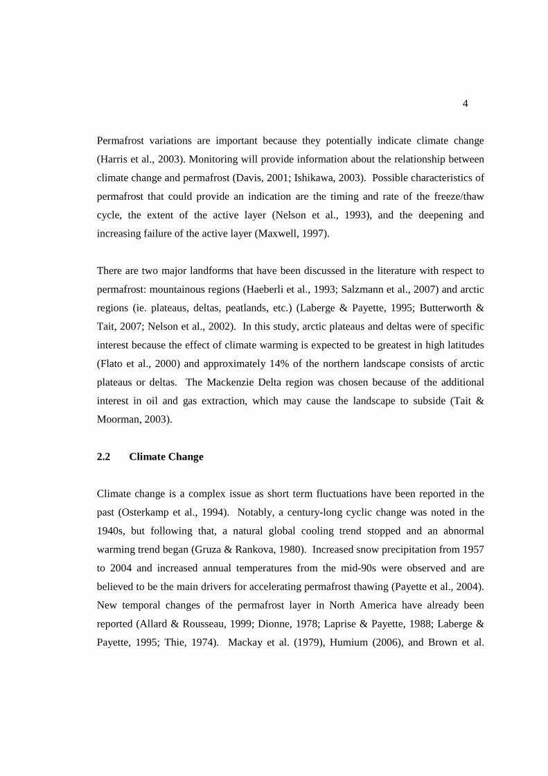
2.3.3 Frost / Thaw Tubes
When using a frost tube, a hole is drilled or bored perpendicularly into the frozen ground,
then a PVC pipe is inserted with a clear plastic tube with inches or centimeters marked
inside of it. The clear tube is then filled with a liquid that changes colour when the soil’s
temperature reaches the freezing point and is then sealed at both ends. When the
measurement is to be made, the user pulls the tube out of the PVC pipe to estimate the
depth of the freezing point. Most frost tubes are approximately 150 cm long.
The greatest benefit of frost tubes is that they provide an inexpensive annual report of the
freezing and thawing of the permafrost active layer. They are also very durable to animal
damage and weathering and they remain very stable as a reference point. Where the layer
is too deep for probing or the ground is saline, fine-textured, or stony, the frost tubes are
ideal because of their stability and durability (Nelson & Hinkel, 2003). Figure 2.6 shows
the construction design of the tube and its positioning relative to the ground.
11
Figure 2.6: Example of a Frost / Thaw Tube
There are two major disadvantages to using frost tubes: accuracy and installation
requirements. The information provided by frost tubes does not indicate the exact dates
of each of the measurements. This hampers the correlation of the measurements with

12
temperature trend data. The installation of a single frost tube requires expensive drilling.
The drilling generally disrupts the surface of the permafrost causing alterations to the
results. Most importantly, the site of the frost tubes needs to be accessible for machinery
and humans to install and maintain each tube. Once the frost tube is installed, one person
is required to collect the data to create a model of the freezing and thawing of the tube.
2.3.4 Ground Penetrating Radar
Ground penetrating radar (GPR) is a ground based system that can be used to determine
the ice’s thickness. Ice is transparent to the microwave radio signals, but ice-sediment
and ice-water interfaces are reflective; therefore, GPR is most effectively used in the
winter in wetland areas.
The properties of permafrost have favourable electrical properties for the use of GPR.
When the soil temperature is below 0oC, the conductivity, the dielectric permittivity, and
the loss tangent tend to decrease, while the velocity of propagation increases (Scott et al.,
1990). These effects mean that the penetration depths also increase, but if there is too
much ice in the soil, there is a reduced ability to detect all the features due to scattering
losses.
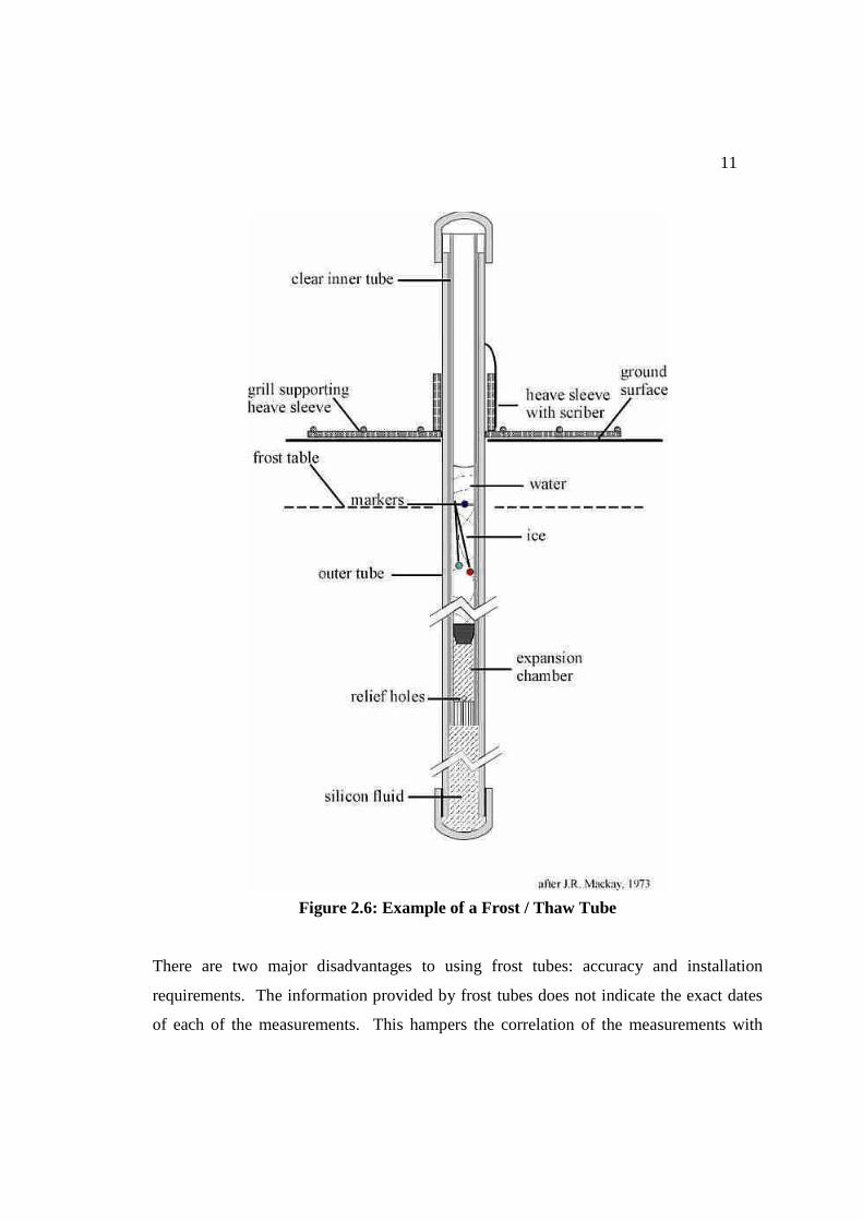
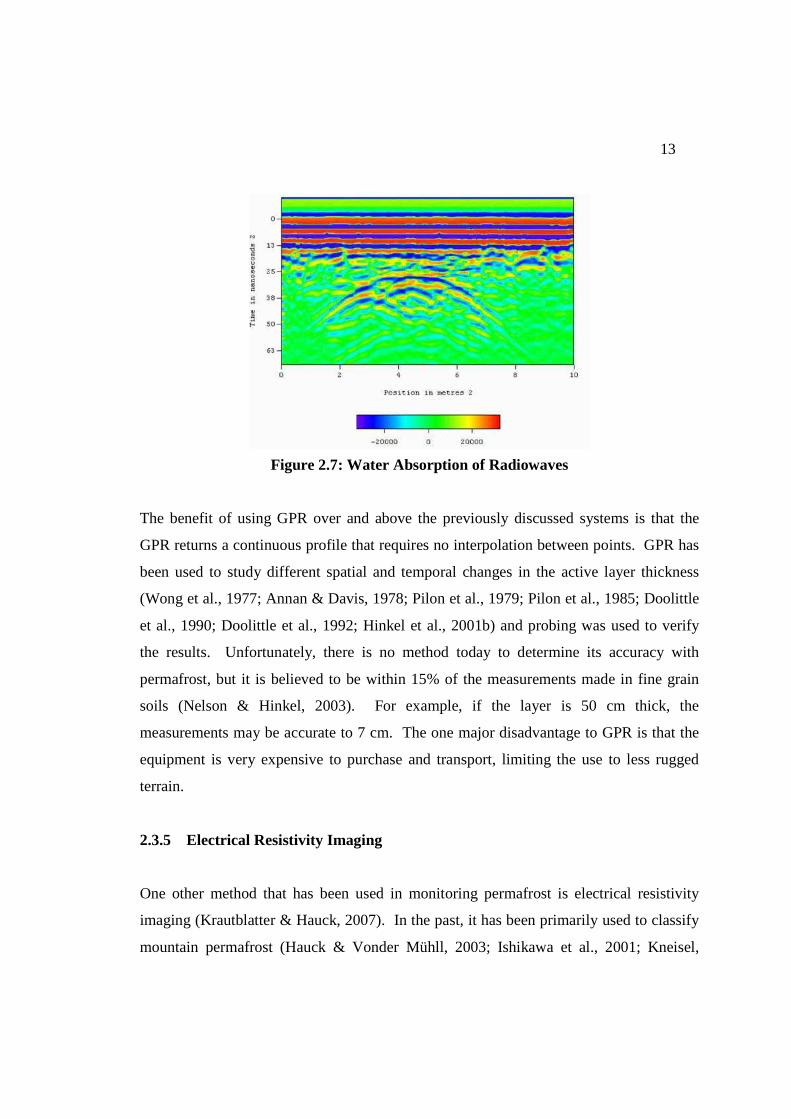
This concept can be seen in Figure 2.7. There are pockets of water that form around the
permafrost regions during the summer and because water absorbs electromagnetic pulses,
the resulting images would not be useful. Insufficient penetration results because of the
water presence during the summer. When GPR is used in the polar regions, it is used
based on the theory that the active layer holds less water than the inactive layer
(Moldoveanu et al., 2003).
13
Figure 2.7: Water Absorption of Radiowaves
The benefit of using GPR over and above the previously discussed systems is that the
GPR returns a continuous profile that requires no interpolation between points. GPR has
been used to study different spatial and temporal changes in the active layer thickness
(Wong et al., 1977; Annan & Davis, 1978; Pilon et al., 1979; Pilon et al., 1985; Doolittle
et al., 1990; Doolittle et al., 1992; Hinkel et al., 2001b) and probing was used to verify
the results. Unfortunately, there is no method today to determine its accuracy with
permafrost, but it is believed to be within 15% of the measurements made in fine grain
soils (Nelson & Hinkel, 2003). For example, if the layer is 50 cm thick, the
measurements may be accurate to 7 cm. The one major disadvantage to GPR is that the
equipment is very expensive to purchase and transport, limiting the use to less rugged
terrain.
2.3.5 Electrical Resistivity Imaging
One other method that has been used in monitoring permafrost is electrical resistivity
imaging (Krautblatter & Hauck, 2007). In the past, it has been primarily used to classify
mountain permafrost (Hauck & Vonder Mühll, 2003; Ishikawa et al., 2001; Kneisel,
14
2006; Kneisel & Hauck, 2003). The idea behind this type of imaging is based on the fact
that at the freezing point, there is an increase in the electrical resistivity of the soil. A
current is injected into the ground using two electrodes and then the voltage difference is
determined. The disadvantages to using electrical resistivity imaging are that any amount
of water in the soil will affect the results and that the readings remain relatively shallow
(Kneisel et al., 2007). Because arctic permafrost can be hundreds of meters deep and
contain a high soil moisture content, this type of monitoring would not be practical.
2.3.6 Circumpolar Active Layer Monitoring
Circumpolar Active Layer Monitoring (CALM) network was established in the 1990’s
and incorporates probing, frost / thaw tubes, soil temperature profiles, and visual
measurements (CALM, 2006). The program originally did not report or archive the data
collected, so the available historical measurement data covers only the past three to five
years. Now, all the data is freely available and provides ground truth data with
approximately 2 cm accuracy (Brown et al., 2000). Linear interpolation is used between
each of the points of measurement.
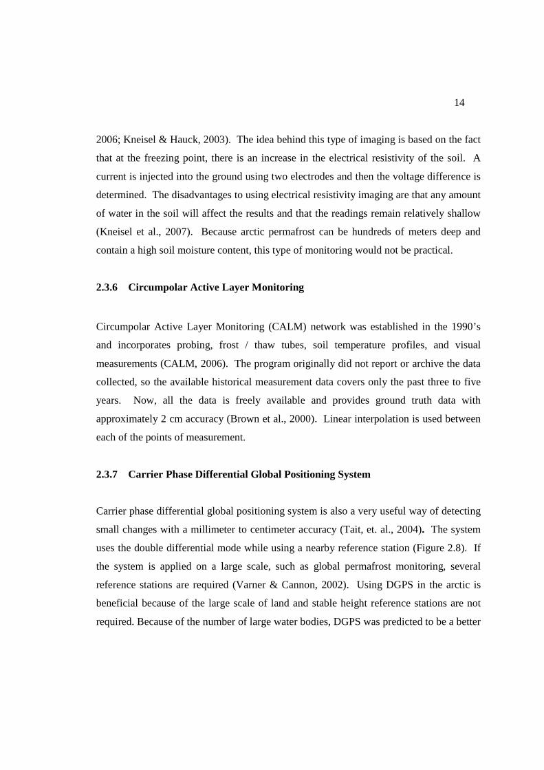
2.3.7 Carrier Phase Differential Global Positioning System
Carrier phase differential global positioning system is also a very useful way of detecting
small changes with a millimeter to centimeter accuracy (Tait, et. al., 2004). The system
uses the double differential mode while using a nearby reference station (Figure 2.8). If
the system is applied on a large scale, such as global permafrost monitoring, several
reference stations are required (Varner & Cannon, 2002). Using DGPS in the arctic is
beneficial because of the large scale of land and stable height reference stations are not
required. Because of the number of large water bodies, DGPS was predicted to be a better

15
option than conventional leveling (Cramer et al., 1999). But again, the problem arises
since the areas to be measured must be accessible.
Figure 2.8: Double Differencing GPS
A disadvantage of differential GPS is that a variety of errors need to be corrected or
compensated for. A few corrections that directly affect the polar regions are (Varner &
Cannon, 2002; Sheng et al., 2007):
- ionospheric activity
- poor satellite geometry
- multipath effects
- phase-center-variation (PCV).
Tait, et. al. (2004) had developed algorithms and methods to reduce these errors to
produce the best results. In the processing of the data, the ionospheric activity value was
considered ionospheric free (because this method combination helped to reduce the
ionospheric errors), an algorithm function provided a map of the troposphere, and a

16
method was developed to reduce the effect of ionospheric activity, poor geometry, and
PCV.
Sheng et al. (2007) found the best accuracy of the DGPS results in the high arctic were
around 2mm +- 8mm, when a receiver was left collecting data for 12 hours.
From the above previously used methods, one can see that each of them require direct
measurements of the soil. This requires accessibility and appropriate weather conditions
to allow for measurements; therefore there are ground observations in only a small
portion of the arctic (Little et al., 2003). Another option is to look for remotely sensed
data, such as aerial or satellite data. These data will generally provide image coverage of
the area, where the spatial accuracy is restricted to the pixel resolution. Remote sensing
via airborne or space borne sensors provides the greatest chance for large scale
monitoring of the permafrost regions (U.S. Arctic Research Commission Permafrost Task
Force, 2003). There are many options available for remotely sensed data, but differential
synthetic aperture radar interferometry (DInSAR) was chosen above all the rest. The
following section explains the reasoning behind this choice and provides information on
the foreseen advantages and disadvantages of this technology.
2.4 Differential Interferometric Synthetic Aperture Radar
DInSAR is another way of monitoring height changes. The first original use of satellite-
based DInSAR was to monitor ground motion in agricultural fields by Gabriel et al.
(1989) and it uses a repeat pass principle to collect the data. The detectable
displacements enter into the sensor directly and therefore can have an accuracy of a
fraction of its wavelength. The actual displacement measurement is considered a
measure of the temporal decorrelation of each pass’s image. Temporal decorrelation can
17
be defined as the phase difference of two signals that are separated by a period of time.
Using these phase differences, one can create a displacement map of a particular area.
The advantages of using DInSAR in the arctic are the accessibility to large areas without
the need of repeated human interaction. It also does not have any lasting effect on the
environment (for example, pathways built, vegetation damaged, permafrost being altered)
and it can remotely monitor large areas without a local point-based system. It is very cost
effective because the satellites are already in orbit and the images are available for use.
But there are disadvantages in using DInSAR in the arctic. A few of problems are the
rapid changes in vegetation between passes, the ionospheric activity and the tropospheric
activity. The processing of the images can be also very difficult.
2.5 Problem Statement
The remoteness and unrelenting harsh environment of the polar regions highlighted the
need to find a new, effective remote sensing method. Large area coverage, high spatial
resolution, and high vertical accuracy cannot be achieved with the techniques mentioned
in section 2.3. To solve these limitations, synthetic aperture radar interferometry
(InSAR) has been proposed as an alternative (Graham, 1974; Zebker & Goldstein, 1986).
Differential synthetic aperture radar interferometry (DInSAR) showed promise and was
chosen for evaluation in this research.
18
CHAPTER THREE
SYNTHETIC APERTURE RADAR INTERFEROMETRY
3.1 Introduction
InSAR is a technique that uses radar pulse echoes to produce a two dimensional image
(Rodiguez & Martin, 1992). Because SAR satellites are active and use microwaves, data
can be acquired either day or night and in any weather condition (Rosen et al., 2000).
When using temporally separated, repeat-pass InSAR, also called differential
interferometric SAR (DInSAR), these radar signals can be used to estimate elevation
changes (Hanssen, 2003), soil moisture (Komarov et al., 2002; Mironov et al., 2005), ice
content of land (Moorman & Vachon, 1998), be used for heat loss mapping (Granberg,
1994), vegetation classification (Hall-Atkinson & Smith, 2001; Granberg, 1994) or
monitor deformation of the ground, as shown in the following four examples of
applications.
1. Earthquake Monitoring. After the 1998 Zhangbei-Shangyi earthquake in China,
precise seismic deformation measurements became a topic of interest. SAR
interferometry was used to show surface deformation. Using the ERS-1/2 SAR
tandem mode data taken before the earthquake, the topographic phase signals were
reduced significantly (Wang et al., 2004). The resulting image demonstrated the
location of the epi-center and the surface deformation after the earthquake resided.
Several papers have been written for earthquake monitoring in the past (for example,
Fialko et al., 2005; Crippa et al., 2006).
2. Land Subsistence Detection. As the earth's population uses large amounts of
subsurface natural materials that are not being replaced as rapidly, the ground surface
will settle or sink. In China, land subsistence has been seen in Suzhou City, because

19
the cities population was using too much ground water (Wang et al., 2004), and a
similar effect is taking place in Central Valley, California in the oil and gas fields
(Fielding & Dupre, 1999).
3. Volcanic Eruptions. The transition period between a volcano being at rest and its
eruption is not fully understood. Using DInSAR, Lu et al. (2002) has found that there
are four deformation processes that occur in the transition period. There also is the
possibility to monitor lava characteristics, according to Lu & Freymueller (1998).
These findings can help provide faster updates regarding the possibility of eruptions
and provide a priori information as to the strength of the upcoming eruption.
4. Glacier Motion. There are several mentions of using DInSAR for studying glacier
motion, only two are mentioned here (Eldhuset et al., 2003; Strozzi et al., 2002). With
concerns regarding the climate change problem, glaciers are among one of the land
features greatly affected by temperature changes and are providing information on the
rate of climate change.
Radar satellites record the phase and amplitude values of the waves. This information
can be used to improve accuracy of determining the magnitude and direction of land
deformation. Horizontal and vertical change detection accuracy can be in the millimeter
level (Wegmueller et al., 2006), but is usually in the centimeter range (Rodiguez &
Martin, 1992).
The most important feature of SAR interferometry is the ability to map remote areas.
Larger areas can be monitored directly, without requiring continual human interaction on
the land, but because the idea of using SAR interferometry for permafrost monitoring is
relatively new, there are some challenges that were involved.

20
The first challenge when using DInSAR is choosing the appropriate images. Temporal
decorrelation and image geometry are two very important attributes to consider when
making this decision (Strozzi et al., 2003). During the early summer to mid-fall, there is
a better possibility of high coherence of the images in the arctic. Once there is snow on
the ground, the images may become inconsistent because of the moisture and density
heterogeneities, which are detected by volume scattering of the microwaves. Because the
purpose of the project is to determine the surface deformation of the permafrost layer,
this is best completed during the summer season, where the surface of the permafrost is
unobstructed by snow.
Temporal decorrelation, image geometry, Doppler centroid differencing, and processing
methodology will affect the coherence of the image. If the coherence of the image is too
low, image registration, phase unwrapping, and the creation of a deformation map will be
affected. Also, coherence must exceed a threshold level, which may not be possible in
certain situations. Coherence will be discussed in greater detail in the next chapter.
Finally, the field information and the mathematical model of the images are among the
toughest challenges. To determine the true permafrost layer, ground elements such as the
different types of vegetation and soil elements must be analysed. Also, several ground-
based reference stations must be visible in the images to provide geographic coordinates
for accurate georeferencing. Atmospheric attenuation and scattering should also be
considered while choosing the image processing method and adjusting for random
frequency scattering (Foody & Curran, 1994). Unfortunately, with time and financial
constraints, the latter was not possible in this study.
The focus of this study is to isolate the above properties and challenges of a differential
interferogram and determine the best approach to monitor vertical movement of
permafrost. There have been DInSAR permafrost studies in the past (Wang & Li, 1999;

21
Li et al., 2003), but the results have not been factor analyzed or correlated with ground
truth data. The factors spoken about here include temporal decorrelation components,
image geometry, and coherence components.
3.2 The Radar Equation
3.2.1 Monostatic Point Scatterer Radar Equation
The governing equation for radar systems is the radar equation. The transmitting antenna
sends a signal of known power, then this signal interacts with the target, and finally the
receiver antenna measures the amount of returned (or backscattered) signal power.
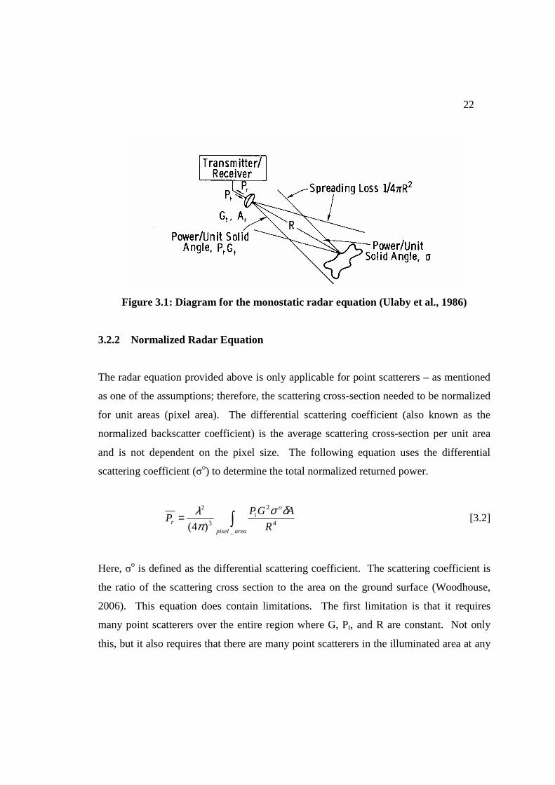
Figure 3.1 provides some insight as how the radar equation works and the following is
the monostatic version of the radar equation.
42
2
43
22
4)4( R
AP
R
GPP att
r πλσ
πσλ
== [3.1]
Where: Pr = power received
Pt = power transmitted
G = gain
λ = wavelength
σ = scattering cross-section
R = slant range
Aa = area of antenna related to gain.
22
Figure 3.1: Diagram for the monostatic radar equation (Ulaby et al., 1986)
3.2.2 Normalized Radar Equation
The radar equation provided above is only applicable for point scatterers – as mentioned
as one of the assumptions; therefore, the scattering cross-section needed to be normalized
for unit areas (pixel area). The differential scattering coefficient (also known as the
normalized backscatter coefficient) is the average scattering cross-section per unit area
and is not dependent on the pixel size. The following equation uses the differential
scattering coefficient (σo) to determine the total normalized returned power.
∫=areapixel
ot
r R
AGPP
_4
2
3
2
)4(
δσπλ
[3.2]
Here, σo is defined as the differential scattering coefficient. The scattering coefficient is
the ratio of the scattering cross section to the area on the ground surface (Woodhouse,
2006). This equation does contain limitations. The first limitation is that it requires
many point scatterers over the entire region where G, Pt, and R are constant. Not only
this, but it also requires that there are many point scatterers in the illuminated area at any
23
instant. In this study, these limitations are assumed in the areas of interest and this
version of the radar equation was used.
The value of the received power per pixel is affected by many factors that affect the
scattering cross-section. A few of these factors that are examined in this study are the
image geometry, temporal decorrelation (including ionospheric effects), Signal to Noise
Ratio (SNR), Doppler centroid, and processing methodology. These five factors are also
used in determining the coherence of image pairs; which was another focus of this study.
3.2.3 Scattering Properties
The radar equation describes the scattering that occurs by a target, therefore an
understanding of the term scattering is required. Scattering can be defined as the
“redirection of incident electromagnetic energy” (Woodhouse, 2006). Words such as
reflection, refraction, and diffraction are more specific types of scattering; where the
word “scattering” refers more to the random change of direction created by elements that
are the same size or smaller than the wavelength. These elements are referred to as
“scatterers.”
A measure of the effectiveness of a scatterer is called the scattering cross-section – seen
in the radar equation as σ. The scattering cross-section is defined by the ratio of the total
scattered power to the total incident power proportionally related to 4πR2. In an image,
the pixel size is the limiting factor here; therefore there is a possibility that the total
scattered power can be affected by one dominant scatterer, as can be seen by the bright
points in Figure 3.2. Therefore, one of the assumptions of the above radar equation is
that the scattering area must consist of randomly placed point scatterers with random
amplitudes; and therefore there must not be a dominant scatterer in the pixel.
24
Figure 3.2: Backscatter power of a group of scatterers in a pixel with dominant
scatterers
3.3 Image Geometry
Image geometry is of great importance in DInSAR processing, therefore understanding
the collection of the data will provide some insight to the physical properties of the signal
processing. The signal processing (or focusing) of the data will not be mentioned here
because the images used were processed by a third party.
The antenna of a SAR satellite transmits and receives signals at an angle to nadir (the line
perpendicular to the earth). This angle is referred to as the incidence angle and is shown
in Figure 3.3 (Hansson, 2001) as θ. The incidence angle can be referenced to three
different locations: at the near range, the far range, or in the center of the beamwidth
(seen as βr in Figure 3.3). In this study, the incidence angle is considered to be in the
center of the beamwidth. There is also another type of incidence angle that is not shown
in the figure, which is referred to as the local incidence angle. The local incidence angle
is the angle the transmitted signal makes with the ground. Depending on the topography,
the local incidence angle can vary greatly from the transmitted incidence angle, creating

25
problems with foreshadowing, shadowing, and layover. However, in this study, the
plateau and delta are relatively flat, decreasing these geometric distortions.
In each acquisition, the incidence angle does not change, but the position of the satellite
does, as marked as positions 1 and 2. This change of location creates the early azimuth
location and the late azimuth location of the footprint. The near range, far range, early
azimuth, and late azimuth define the resolution of the pixel. The azimuth resolution is
half the length of the antenna (La); therefore, the smaller the antenna is, the better the
resolution. The range resolution is determined by the height of the satellite (Hsat) and the
beamwidth (Hanssen, 2001).
Figure 3.3: Image acquisition geometry for a single pixel

26
In non-imaging SAR applications, the incidence angle is used to determine information
about the radar cross section (Woodhouse, 2006). But in imaging SAR applications, the
balance of backscattering power and reduction of geometric distortions (such as
foreshadowing, layover, and shadowing) is directly dependent on the chosen incidence
angle. An angle of 45o has been previously recommended (Bamler & Hartl, 1998), but in
this study, a range of lower values from 28o to 39o had been chosen to enhance the ability
to detect vertical change, by keeping the deformation close to the line of sight. It was
expected that the signal to noise ratio would be higher for these lower incidence angles
because as the angle decreases, the SNR increases. But if the incidence angle is not
chosen properly, the returned values of the radar cross-section will change, affecting the
coherence between two images.
3.2.1 Baseline Geometry
Once two images of the same area have been acquired, there was one other factor of
image geometry to examine: the baseline (Figure 3.4). The baseline is the physical
separation of the two satellites while acquiring the same image. The maximum value
between satellites that is recommended is 500 m (Li & Goldstein, 1990); otherwise the
coherence is reduced. The baselines are dependent on each satellite’s individual orbit and
therefore cannot be pre-determined.

27
Figure 3.4: Baseline geometry
The radar information must be derived from simple trigonometry by using the distances
between two sensors (the baseline) and the resolution cell (the range). In three-pass
interferometry, the important factor to consider in the imaging geometry is the baseline
correction. In the case of baseline correction, we are examining the spatial baseline
because of the high demands on geometric configuration of the interferometric method.
The baseline can be used to determine the change in range between the two sensors, but it
cannot be used primarily because of the 2π phase ambiguity. If the second sensor is
found to the right of the first sensor in terms of flight direction (refer to Figure 3.3), the
baseline will be positive and the change in slant range will change from near range to far
range.

28
In developing interferograms, each point / pixel in the image requires a reference phase to
correctly register the images. A simple overlay used in image processing would not be
sufficient for the complex radar data. Therefore, using the total baseline (B),
perpendicular baseline (Bp), the range of the first sensor (R), the height of the point (Hp),
the look angle (θ), orientation angle (α), and the displacement of the point (Dp), the
reference phase can be determined (Equation 3.3):
)sin
)sin((4
pp
pp HR
BDB
θαθ
λπφ −−−= (Hansson, 2001) [3.3]
In using this equation in the differential processing, a baseline of 100 meters and a height
difference of 1 cm, the phase difference is found to be 127 degrees. This difference is
easily detectable in an image. If the displacement is in the line of sight, it is independent
of the baseline and can be measured as a fraction of the wavelength. If the baseline is
non-zero, as in this study, there is some sensitivity due to the topography.
In the case of a single interferogram, the topographic errors can be determined using the
calculated baseline errors. Using least squares estimation and precise orbit data, the
following equation was used to calculate the topography residuals:
hvnb
vn
B
bnR
B
dh ˆ)ˆˆ(ˆ
ˆˆ)ˆˆ( ⋅×⋅
×⋅−=δ
(Muellerschoen et al., 2006) [3.4]
Where n is the unit look vector, b is the baseline direction, v is the velocity variation,
and h is the local vertical at the target point.
In this study’s processing, the baseline between the interferometric pairs needed to be
taken into account and scaled. This was done once the reference phase (Equation 3.3)

29
had been subtracted from both interferograms. The phase observations in the
interferogram are considered to be the sum of phase due to distance and the phase due to
the backscatter, as long as atmospheric delay is not considered. But in this study, the
influence of the atmospheric signal delay must be considered. The atmospheric delay has
only one contribution for each pixel in the master (common) image and because the
scaling factor (Bdef/Btopo) scales the pair that creates a digital elevation model (DEM)
(called the topographic pair), the atmospheric signal is scaled in the same respect. This
scaling is important in the analysis of the final differential interferogram and when the
unwrapped, scaled topographic pair is subtracted from the remaining pair (called the
deformation pair); a differential pair would be created showing only deformation.
The model of the observation equations to calculate the deformation is as follows
(Hanssen, 2001):
=
Ω−
Ω−
mm
wIIm
wII
wII
Im
I
I
m x
x
x
A
A
A
EMO
M
M
OO2
1
2
1
2
1
2
1
1
1
1
φ
φφφ
φφ
[3.5]
Where A is the differential design matrix including atmospheric parameters, which are
clearly affected by the baseline scaling factor (Ω). A large scale needs to be avoided
otherwise the atmospheric signal is amplified. To reduce the atmospheric signal, the
scaling factor must be between zero and one; otherwise the signal will be amplified
(Bracewell, 1986). Therefore the topographic pair needs to have these characteristics:
30
1) a larger baseline than the deformation pair;
2) have a baseline smaller than 70% of the critical baseline; and,
3) contain terrain relief, vegetation, and temporal decorrelation.
In all the sets of data, the June/July pair was used as the topographic pair. In set 3, the
topographic pair did not have the longest baseline, which will have amplified the
atmospheric delay.
If one is interested in learning more, there are many papers available to provide
additional information on this processing (Bamler, 1992; Cumming & Wong, 2005; Hein,
2004; Ulaby et al., 1986).
3.4 Temporal Decorrelation
Temporal decorrelation is defined as differences of the phase and amplitude of the radar
signals between passes. It is caused by the radar signal detecting a change in surface
properties (also known as the radar cross-section (Wegmueller & Werner, 1995)) or a
change in atmospheric / ionospheric effects (Hanssen, 2001) over a particular time
period. Northern environments have rapidly changing vegetation because of the short
growing season (Billings, 1987). Therefore many changes in the radar cross-section
between orbits can be detected. The radar cross-section can be affected by moisture
content and dielectric constant values and can cause a phase difference between each
acquisition (Woodhouse, 2006). One option to try to improve coherence is to use
polarimetry measurements to model the changes in the radar cross-section over time.
This option would not only allow for modeling the radar cross-section changes, but
would also provide the optimal incidence angle.
31
Two other factors in temporal decorrelation are the atmospheric and ionospheric changes.
As a radar signal travels through the atmosphere, it can be refracted or delayed in each
layer. These effects depend on the density of the molecules within each layer. The
atmosphere was first reported to be an influential factor on SAR imagery in 1995 by
Goldstein (1995), Massonnet & Feigl (1995a), and Tarayre & Massonnet (1996). There
are mathematical models available that describe how the atmosphere stochastically
affects SAR interferometry (Hanssen, 2001; Massonnet & Feigl, 1995b]; but presently
there are no methods available to measure the delay caused by the atmosphere to the
required accuracy, spatial resolution, and temporal resolution of this study.
3.4.1 Ionospheric Activity
The ionospheric activity was observed because of the known increased activity in
northern environments. The electron density within the ionosphere is often generalized
as a spherical shell and is not considered temporally and spatially variable (Hanssen,
2001). High electron activity tends to decrease the range and cause a phase advance of
the radar signal because of the interaction with the electrons. A decrease in ionospheric
water vapour also tends to increase the range, therefore causing more of a phase advance.
Dual-frequency GPS has been used to estimate the ionospheric delay (Hanssen, 2001),
but a strong satellite geometry is required (Sardon et al., 1994). It was found that DGPS
has a poor geometrical configuration in the Arctic and therefore using DGPS to model the
ionosphere is not possible for specific times and locations (Sheng et al., 2007).
The town of Yellowknife, Northwest Territories, has an observatory that provides
information on magnetic activity in the ionosphere. This information was collected and
analyzed for the purposes of this study. Gray et al. (2000) was the first to prove that
ionospheric activity affects the radar signal in the arctic, but the magnitude and validation
of this effect were lacking in their study. At this time, the hypothesis used is that the

32
ionosphere may cause long wavelength gradients over one image, but will not be
noticeable in images with a scale less than 50 km.
3.4.2 Example of Atmospheric Disturbances
Hanssen & Feigt (1996) had completed a study to assess if the atmospheric delay in
InSAR could be modelled using GPS measurements. The GPS signal was affected by the
troposphere in the same way as the radar signal and it was hypothesized that a GPS
derived model could be used to quantitatively calculate the signal delay in InSAR. It was
found that using GPS to correct the InSAR atmospheric delays was very difficult. The
GPS baselines were too noisy and could only be crudely filtered. The correction was also
very dependent on the spatial distribution of the GPS receivers. The results of the study
also determined that the GPS signal, at a 20 degree elevation, will cover a large area
around the receiver; therefore, the gathered data did not provide enough information to
remove the small artefacts from the radar signal. In the arctic, the elevation angle is
much lower and therefore the atmospheric delay information will cover a much larger
area around the GPS receiver. Also, in deformation studies, such as this one, the small
scale of deformation could not be determined by the GPS and attempting to filter the
SAR interferogram would continue to leave all atmospheric and deformation signals.
But, it was found that GPS could be used to parameterize the atmospheric signal in the
SAR interferogram. Because of the remoteness of the arctic, it would be difficult and
very expensive to set up such a network of GPS receivers and would negate the value of a
remote sensing method to monitor permafrost.

33
3.5 Signal to Noise Ratio (SNR)
The antenna in a satellite system tends to pick up noise from external and internal sources
in addition to the image footprint. These noises can come from other microwave sources
or from the satellite system itself (such as an electrical leak or a result of the temperature
of the instruments) (Woodhouse, 2006). To define the general usefulness of a system, a
signal to noise ratio (SNR) is used:
signalunwanted
signalwantedSNR
_
_= [3.6]
So if the SNR is less than one, the system is receiving less useful signal power than noise
power, but if the SNR is high, then the system is performing well. The SNR is governed
by the radar equation, which relates received power to transmitted power. Often, the
radar equation will be seen written in terms of the SNR of the final image to determine
the required imaging quality (Cumming & Wong, 2005). When trying to calculate SNR,
equation 3.7 can be used:
isnT
ave
VLFKTBR
cGPSNR
o
θπσλ
sin256 33
32
= [3.7]
Where: Pave = average transmitted power
G = Antenna gain
λ = wavelength
σo = backscatter coefficient
c = speed of light
R = Range to reflector
K = Boltzmann’s constant
34
T = temperature of receiver (K)
BT = transmitted signal bandwidth
Fn = receiver noise figure
Ls = system losses
V = platform velocity
θi = incidence angle
From the equation, one can see that the SNR is inversely proportional to the range of the
signal.
When the SNR value is too low, the coherence of an image is affected. This will cause
difficulties in registering the images and with phase unwrapping. More information on
how the SNR affects the coherence will be discussed later. Unfortunately, the SNR
cannot be controlled or predicted in advance and is calculated in the image registration
step.
3.6 Doppler Centroid Differences
The Doppler effect occurs in the azimuth direction of the signal footprint. It is
proportional to the velocity of the antenna and inversely proportional to the velocity of
the radar waves spreading (Hein, 2004). Radar imagery encounters a special form of the
Doppler effect called the Doppler centroid frequency. The Doppler centroid frequency is
a linear, additive frequency function that communicates the encountered frequency
displacement. Once simplified, the Doppler frequency can be calculated by:
βλ
sin2 ⋅⋅= resD
vf [3.8]
Where: vres = effective velocity of the sensor

35
λ = signal wavelength
β = beamwidth
This equation is a relationship between the beam center location and the returned signal
energy in the flight direction (Hanssen, 2001). The Doppler centroid is calculated as the
satellite passes through the beam center of the target. This is the point where the
acquisition has the maximum gain and can be estimated using a geometric model with the
satellite orbit and attitude data. Unfortunately, for the purposes of most research, this
method of calculation is not accurate enough. To accurately determine the Doppler
centroid, the received signal data is required (Cumming & Wong, 2005) and can only be
estimated after the image acquisition.
The difference of the Doppler centroids of two registered pixels is ideally close to zero.
As the difference increases, the coherence will decrease (Swart, 2000; Hanssen, 2001).
This effect will be discussed in a later section.
3.7 Processing Methodology
Although the processing methodology does not affect the true returned signal, it does
affect the quality of the image and the resulting values of the pixels. Errors may result
from the chosen method in a processing step. The decorrelation is a result of phase
aberrations that can be introduced through spectral misalignment (Bamler & Just, 1993).
Spectral misalignment is generally referred to as two images having a phase variance
(Bamler & Just, 1993). The images will result in similar scatterers improperly aligned
during the processing (Hein, 2004). The misalignment can be a result of two different
steps (Eldhuset et al., 2003): geometric misregistration and interpolation methods.

36
3.7.1 Geometric misregistration
The geometric misregistration can occur in either the range or azimuth direction
(Eldhuset et al., 2003). It causes a phase variance and it depends on a displacement of the
scatterers (Hein, 2004). If the misregistration is larger than one pixel, the coherence will
equal zero; therefore it is recommended that the registration be accurate within at least
1/8 of a pixel (Hein, 2004) before continuing.
In this study, there were two options for image registration: intensity cross correlation
algorithm and fringe visibility algorithm. The intensity cross correlation algorithm uses
the intensity values of each pixel in the images and correlates them according to the
equation:
∑∞
−∞=
−×=n
xy inynxiR )()()( [3.9]
Where x and y are the pixels to be cross correlated, i is the iteration, and n is the signal’s
phase shift. The equation overlaps all the elements of the two image’s signals and sums
everything with the appropriate phase shift. The offset of the intensity peaks shows the
phase difference (and therefore the misregistration) for each pixel (Denbigh, 1995). One
of the benefits of the intensity cross correlation algorithm is that it allows for any two
images to be registered.
The other registration algorithm that was examined was the fringe visibility algorithm.
Before using this algorithm, interferometric fringes must be visible in the images. These
fringes occur in a 2π cyclic pattern and in the case of radar fringes, the image must
exceed the 2π pattern. To determine the visibility of the fringes in each image, equation

37
3.10 must be used, where I is the irradiance, b is a function of the image spectral filter,
and ro is the complex amplitude of the reference image beam.
2
2minmax
minmax
1
2
o
o
rb
rb
II
IIV
+=
+−
= [3.10]
Once the visibility of the fringes in each image has been determined, Fourier transform
integrals are used (Anderson, 1995). Equation 3.11 was used in this study:
R
yxjWSyxr oofoo
λγξππγξ )](2exp[),(
),(2 +
= [3.11]
Where: r(x,y) = the master image signal value
S(ξo,γo) = the Fourier filter plane
Wf = the filter size
x & y = pixel numbers
λ = wavelength
R = slant range
The above equation is then applied to the second image (the slave image) and the fringes
are matched. The requirement for this algorithm is that there needs to be an initial
interferometric correlation between the two images, which may not be the case in all
studies. The fringe visibility algorithm is computationally more expensive and tends to
have a very small filter size, only allowing it to cover a few pixels at a time, but because
it requires initial correlation between the images, the coherence tends to be higher.

38
CHAPTER FOUR
COHERENCE AND PHASE UNWRAPPING
4.1 Coherence
Coherence is the measure of the extent to which two reflected radar signals are correlated
through phase differences. These values are between zero at low coherence and one at
high coherence. In areas of low coherence, problems can arise in creating digital
elevation models (DEMs) or interferograms (Abdelfattah & Nicola, 2003). Coherence is
affected by several different factors (Zhang & Prinet, 2004; Hanssen, 2001) such as the
ones described in the recent sections.
Coherence is a scalar product that consists of six parameters (Abdelfattah & Nicola,
2003) which include:
1) Sensor parameters such as the wavelength, noise, and resolution;
2) Imaging geometry parameters such as baseline and incidence angle in
interferometric applications; and,
3) Target parameters, such as volume and temporal changes.
Equation 4.1 presents how coherence can be calculated:
processtemporalthermalvolumefdcgeomtotal γγγγγγγ = [4.1]
where: γtotal = total coherence
γgeom = imaging geometry
γfdc = Doppler centroid difference
γprocess = processing methodology

39
γthermal = thermal noise
γvolume = volume of scatterer
γtemporal = temporal decorrelation
To provide a simpler explanation of how coherence works, Figure 4.1 shows an example
of four pixels in an area taken at two different times. Three of the pixels are the same and
are therefore said to have high coherence. The bottom right hand pixel is different. If a
threshold is set at 0.25 and the two pixels have coherence less than the 0.25, they are
considered to have low coherence. Otherwise, if the pixels have coherence above 0.25,
they are considered to have high coherence. A couple factors that could cause low
coherence are a body of water forming within the pixel area or a rapid change of
vegetation.
Figure 4.1: Example of pixel coherence
4.1.1 Imaging Geometry
When imaging geometry affects the coherence of a SAR image, it is generally due to the
difference in the baseline or incidence angles of two sensors (Hanssen, 2001). When the
baseline becomes too long and the spectral shift is equal to the bandwidth, then the two
40
images will lose all coherence and reliability; but if the baseline is too short, the
interferometric technique will lose its ability to calculate three dimensional imagery. To
define the maximum length a baseline can be, a critical value must be stated. The critical
baseline value can be defined as:
)tan(')/( ζθλ −=⊥ incprcrit RcBB [4.2]
where: Bcrit = Critical baseline (m)
λ = Wavelength (m)
Br = Data rate (kb/s)
c = Speed of light (m/s)
R'p = Slant range (m)
θinc = Incident angle (rad)
ζ = Reflected angle (rad)
Data rate is defined as the rate information (in bits) can be transported. If the value of the
baseline is larger than the critical baseline, the geometric coherence is defaulted to zero
(Hanssen, 2001). Using the assumption that the baseline is smaller than the critical
baseline value, we can also define the value of the correlation coefficient in equation 4.3
where B is the orthogonal baseline projection of one sensor to the other image’s slant
range (Li & Goldstein, 1990).
crit
critgeom B
BB
⊥
⊥⊥ −=
)(γ [4.3]
41
4.1.2 Doppler Centroid Differences and Noise
The Doppler centroid frequency is related to the azimuth beam center and it locates the
azimuth signal energy to provide the best signal-to-noise ratio (European Space Agency,
2006). A difference between the Doppler centroids of two images will cause the
coherence to decrease. When the difference of the Doppler centroid is larger than the
bandwidth in the azimuth direction, there will be no correlation between the images and,
therefore, will equal zero (Hanssen, 2001). Otherwise, the value of the decorrelation can
be modeled by
A
DCDC B
f∆−= 1||γ [4.4]
where: DCf∆ = Doppler centroid frequency
BA = Bandwidth in azimuth direction
When the average Doppler value is determined in the image during processing, then
azimuth filtering is not necessary. But whether filtering is required or not, the effect of
the processing methodology on coherence also can be calculated. One way of calculating
the coherence of part of the processing methodology is in the coregisteration step, which
can be done using equation 4.5, where µ is the relative pixel shift:
πµ
πµγ )sin(|| =process [4.5]
Thermal noise is theoretically determined with the signal to noise ratio (SNR) (Hanssen,
2001) and is determined through the ratio of the signal power ( rP ) from the radar
42
equation (equation 3.1) and the thermal noise power ( nP ). Then, using the signal to noise
ratio, γthermal is determined to be:
11
1−+
=SNR
thermalγ [4.6]
4.1.3 Temporal and Volume Decorrelation
As mentioned earlier, temporal decorrelation is one of the biggest problems with InSAR
calculations. Unfortunately, because of the number of options and applications of the
temporal decorrelation, there is no single analytical model available to describe the
correlation coefficient. The best way to approach each application and limit the effect of
temporal decorrelation is to collect images with little or no moisture content (SLAM,
2006), use tandem pairs (Knopfle, 1999), or take other measurements, such as GPS
measurements, to obtain atmospheric or land deformation information (Rosen et al.,
1996). Without these corrections, the SNR and coherence will decrease. In this study,
none of these three options for reducing the decorrelation effect were possible; therefore,
corrections were not applied.
Volume decorrelation depends strictly on the wavelength of the signal and the scattering
mediums (Hanssen, 2001). It is caused by refraction of the radar waves within the target.
Again, there are so many different scattering mediums and applications that there is no
general analytical model available to describe it. In this study, the volume decorrelation
was determined to not have a large effect on the results because of the low vegetation and
lack of snow coverage.

43
4.1.4 Coherence Estimation
Each of the above parameters needs to be calculated for each pixel in an image, and then
coherence can be estimated for the pair of images. Coherence estimation windows are
commonly used in InSAR processing. They are defined as using a spatial average on a
sample coherence area (Zhang & Prinet, 2004). Any biases that are found in an image
can be neglected when a large estimation window is used and when the averaged number
of the sample coherence estimation satisfies any a priori requirements. Here the
coherence estimation value is independent of the number of looks. A great way to reduce
the coherence estimation variance is to average as many pixels as possible in the constant
coherence areas (large coherence estimation window) (Eldhuset et al., 2003).
A small estimation window tends to bias any low coherence values to a high coherence
value. The largest problem that arises because of the tendency towards one number is
that the discrimination between coherent and incoherent areas will be difficult. So a
larger estimation window will help to decrease the bias. Although the larger estimation
windows will decrease the absolute coherence values and the range resolution, the data
will become more reliable (Hanssen, 2006). But if the estimation window is too large or
if the area is not homogenous, too much information will be lost or the final coherence
value of the estimation window could be poorly located in comparison to the true image
values (Elhuset et al., 2003).
4.2 Phase Unwrapping
One of the most sensitive steps of DInSAR processing is the phase unwrapping step.
Phase unwrapping converts the observed relative phase signal which has a 2π modulus
interval of [-π, π) to the unknown absolute phase signal. It is for this step that poor

44
coherence, low SNR, poor registration, and poor image filtering will become a problem.
Phase unwrapping depends on the wrapped fringes created when the interferogram was
generated. The error in phase unwrapping comes from the miscounts of the fringe order;
therefore quality input and using the appropriate algorithm is essential for quality results
(Gutmann & Weber, 2000). A wrapped interferogram displays repetitive phase fringes in
an order of 2π. When a phase unwrapping error occurs, fringes are missed or counted
more than once.
There are many different phase unwrapping algorithms available. They can be separated
into two groups: path-following methods and minimum-norm methods (Ghiglia & Pritt,
1998). The most commonly used methods are the path-following methods, especially the
Goldstein’s branch cut algorithm (Gutmann & Weber, 2000). The Goldstein’s branch cut
algorithm is controlled by phase discontinuities; otherwise known as residues (Goldstein
et al., 1988). A path is formed by connecting an equal number of negative and positive
discontinuity sources using a pairwise connection (Gutmann & Weber, 2000). Neutral
discontinuity sources (neutrons) are used to direct the pathway through the negative and
positive sources. These connection lines are referred to as branch cuts pointing from
positive to negative sources. The connection lines continue through a 2π cycle until there
are an equal number of positive and negative sources, to make the path neutral. The
unwrapping algorithm is then not allowed to cross these connection lines.
The connection line formation does not have a unique solution; therefore a set of criteria
are required to create a repeated answer. One of the criteria is to decide on a minimum
cut length threshold (Cusack et al., 1995). Another criterion is to use a low-pass filter
separately on each the cosine and sine sections of the phase wave to reduce the number of
object discontinuities and increase the SNR (Ghiglia & Pritt, 1998; Winter et al., 1993).
The minimum cut length threshold is the simplest criterion to implement of the two

45
options. Creating the connection lines is the most time and computationally expensive
part of creating an interferogram, therefore simpler computations are generally adopted.
Once the connection lines are created, then the image can be unwrapped. The
unwrapping occurs along these lines, starting from the positive source to the negative
source. Then, to create a continuous image, bridges are created and are placed over the
connection lines. This step allows the algorithm to unwrap areas that did not have
connection lines, creating a fully unwrapped image.

46
CHAPTER FIVE
DIFFERENTIAL INTERFEROMETRIC SYNTHETIC APERTURE RAD AR
5.1 DInSAR Background
Once phase unwrapping is successful for each interferogram, differential interferometric
processing can begin. It is at this point where one can attempt to detect the vertical
change in land surface. To visualize how DInSAR works, one can imagine two
temporally separated images traveling along the same orbit path (baseline = zero). When
subtracting one image from the other and if the land surface height has not changed
within fractions of the wavelength, the difference will be zero. If there was a change in
the land, there will be a phase difference detected.
5.1.1 DInSAR Geometry
Figure 5.1 (Woodhouse, 2006) show the geometry of DInSAR. The important factor to
examine is the change in slant range, given by:
)sin( ζθ −= iR mD [5.1]
where |m| is the magnitude of the motion vector and ζ is the direction of the motion
vector from the horizontal.
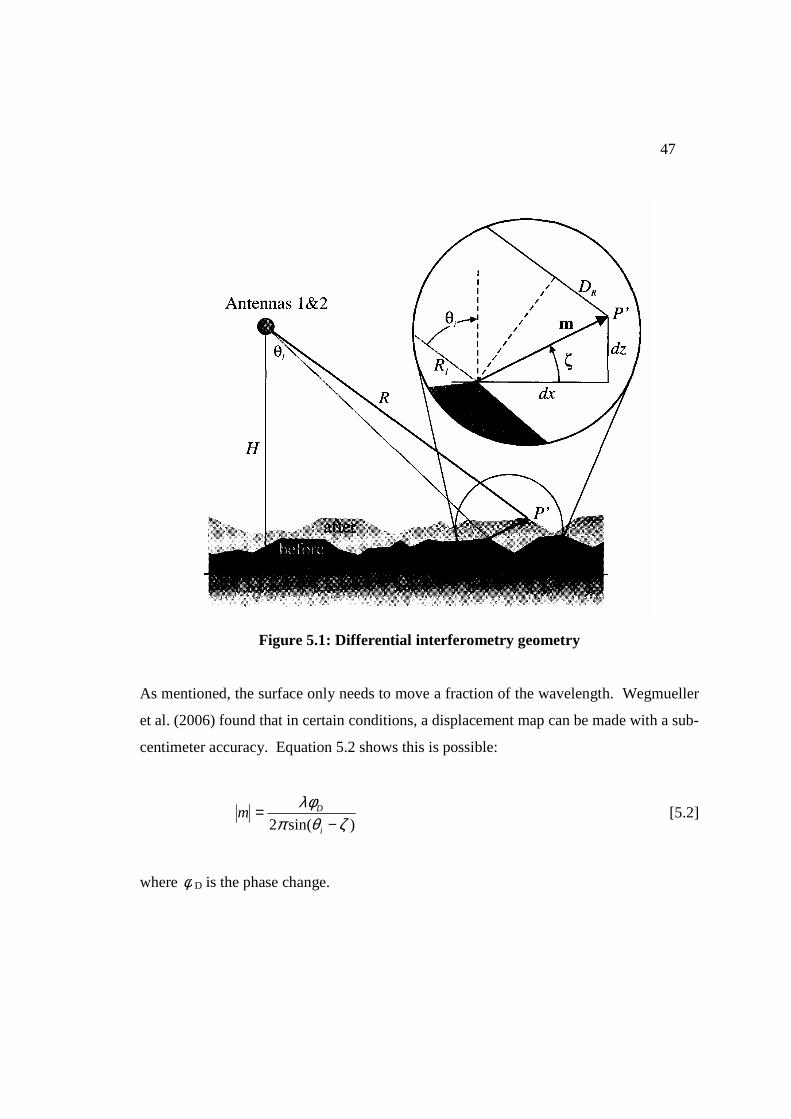
47
Figure 5.1: Differential interferometry geometry
As mentioned, the surface only needs to move a fraction of the wavelength. Wegmueller
et al. (2006) found that in certain conditions, a displacement map can be made with a sub-
centimeter accuracy. Equation 5.2 shows this is possible:
)sin(2 ζθπ
λφ−
=i
Dm [5.2]
where φ D is the phase change.

48
If there is a consistent phase change over the surface and if the area of the ground
movement is found to be larger than the coherence estimation window, the coherence will
remain high (Woodhouse, 2006). Otherwise, the small phase changes found within a
coherence estimation window will decrease the overall coherence values.
5.1.2 Differential Interferogram Computations
There are three options available for computing a differential interferogram: two-pass,
three-pass, or four-pass interferometry.
5.1.2.1 Two-Pass Differential Interferometry
Two-pass differential interferometry uses one interferogram and relates the interferogram
to a previously calculated DEM. The DEM has to be accurate to about 30 meters in the
height direction to be used; therefore GTOPO30 and SRTM data can be used. Thirty
meters is considered accurate enough because the DEM is used only as a reference for
each pass. The objective of two-pass DInSAR is to determine the difference between
each pass with respect to the DEM. There are several examples of two-pass
interferometry in literature, such as monitoring earthquakes (Zhang & Cheng, 2005),
volcanoes (Lanari et al., 1996; Stevens & Wadge, 2004), and glaciers (Rao et al., 2004).
This technique is the most robust and accurate technique, when there is a DEM available
(Zhen et al., 2003). If there is not a DEM available, there is a possibility to use three-pass
interferometry.
5.1.2.2 Three-Pass Differential Interferometry
Three-pass differential interferometry uses three images, which are converted into two
interferograms, with one common reference image (also known as the master image).

49
One of the requirements of this method is there cannot be any deformation between two
of the images or that there is a constant rate of change between all three images. If there
is no deformation found between two of the images, the resulting interferogram is called
the topographic image. Otherwise, the pair of images with the longest baseline is referred
to as the topographic image. In this study, it was found that the deformation had a
constant rate of change using the permafrost heave model. More information on this can
be found in section 6.3.2.
The other interferogram is called the deformation image and is used for the calculation of
the total deformation. These two interferograms are then registered with each other and
the phases are subtracted from one another. This creates the differential interferogram.
The benefit of using three-pass interferometry is that a DEM is not required for the
processing. Because the interferograms need to be registered, the coherence is required
to be higher than in two-pass interferometry; otherwise they may not register together
properly. Also, both interferograms need to be unwrapped before being taken any
further. There are not as many applications of three-pass interferometry; it has been used
in mining subsidence applications in the past (Carnec & Delacourt, 2000), which is
similar to this study.
5.1.2.3 Four-Pass Differential Interferometry
Another common option for DInSAR processing is four-pass interferometry. In four-pass
interferometry, four radar images are used to create two interferograms, but only the first
interferogram is unwrapped. This interferogram is required as the topographic estimation
so it cannot contain any deformation (Zhen et al., 2003). In a subsidence application, this
may be difficult to achieve.

50
5.2 Objectives
This study is a feasibility study that will help to assess the use of DInSAR in monitoring
permafrost subsidence at centimeter accuracies. In this study, three pass differential SAR
interferometry is used to determine the subsidence of permafrost in the MacKenzie Delta
& River Valley region to a centimeter accuracy. DInSAR is capable of sub-centimeter
accuracies, but because of the temporal decorrelation and unaccounted atmospheric
effects, it is expected to see a bias. Field observations occurred during the same time
period as the radar image acquisitions. These field observations include conventional
leveling and data collection for a permafrost heave model, including soil moisture, soil
content sampling, and surface temperatures and are to be used in determining the
accuracy of the remote sensing application.
If proven possible, DInSAR can be used as a seasonal measure and as a monitor for
permafrost subsidence.
The following are the objectives of this study:
1. Create four displacement maps with centimeter accuracy from the radar images;
2. Correlate the pre-calculated conventional leveling DEM and the permafrost heave
model with the radar displacement maps; and,
3. Analyze the factors that caused errors in the DInSAR results.
If one of the DInSAR images provides a displacement map that is verified by ground
data, then using a factor analysis, the optimal conditions for monitoring permafrost
subsidence due to climate change using DInSAR can be determined.
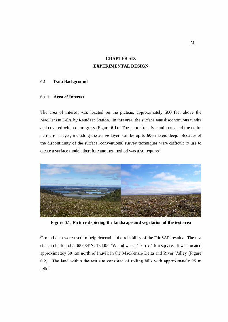
51
CHAPTER SIX
EXPERIMENTAL DESIGN
6.1 Data Background
6.1.1 Area of Interest
The area of interest was located on the plateau, approximately 500 feet above the
MacKenzie Delta by Reindeer Station. In this area, the surface was discontinuous tundra
and covered with cotton grass (Figure 6.1). The permafrost is continuous and the entire
permafrost layer, including the active layer, can be up to 600 meters deep. Because of
the discontinuity of the surface, conventional survey techniques were difficult to use to
create a surface model, therefore another method was also required.
Figure 6.1: Picture depicting the landscape and vegetation of the test area
Ground data were used to help determine the reliability of the DInSAR results. The test
site can be found at 68.684˚N, 134.084˚W and was a 1 km x 1 km square. It was located
approximately 50 km north of Inuvik in the MacKenzie Delta and River Valley (Figure
6.2). The land within the test site consisted of rolling hills with approximately 25 m
relief.

52
Figure 6.2: a) Map of the area where the star represents the area of ground truth
data and the rectangle is the area of image b; b) Intensity image of the same area
where the white square represents the ground truth data area
6.1.2 Images
For the purposes of this work, nine images from the Advanced SAR (ASAR) sensor on
ENVISAT and three RADARSAT-1 images were used. All 12 single look complex
(SLC) images were acquired between the dates of June 18, 2005 and September 8, 2005
and were all in descending node with a frequency of 5.3310044e+009 Hz. The
ENVISAT ASAR images were separated into triplets, with 501 orbits or 35 days between
each image. Table 6.1 shows how each dataset was separated. The images were chosen
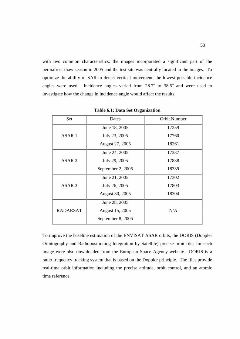
53
with two common characteristics: the images incorporated a significant part of the
permafrost thaw season in 2005 and the test site was centrally located in the images. To
optimize the ability of SAR to detect vertical movement, the lowest possible incidence
angles were used. Incidence angles varied from 28.7o to 38.5o and were used to
investigate how the change in incidence angle would affect the results.
Table 6.1: Data Set Organization
Set Dates Orbit Number
ASAR 1
June 18, 2005
July 23, 2005
August 27, 2005
17259
17760
18261
ASAR 2
June 24, 2005
July 29, 2005
September 2, 2005
17337
17838
18339
ASAR 3
June 21, 2005
July 26, 2005
August 30, 2005
17302
17803
18304
RADARSAT
June 28, 2005
August 15, 2005
September 8, 2005
N/A
To improve the baseline estimation of the ENVISAT ASAR orbits, the DORIS (Doppler
Orbitography and Radiopositioning Integration by Satellite) precise orbit files for each
image were also downloaded from the European Space Agency website. DORIS is a
radio frequency tracking system that is based on the Doppler principle. The files provide
real-time orbit information including the precise attitude, orbit control, and an atomic
time reference.
54
When choosing these images, there were two different landforms of interest. Each image
consisted of the plateau, where the ground truth data was taken, and the active delta. The
delta was of interest because of present and planned commercial gas extraction that may
lead to additional subsidence of the land. If the differential interferogram is successful in
the delta, DInSAR could be used as a potential long term monitoring tool for many
companies. The plateau was used as a dry land comparison. Each of these landforms
represents approximately 7 – 8% of the arctic region.
6.2 SAR Processing
A thorough investigation was completed to acquire the most appropriate software for
radar interferometry processing. Most of the software packages investigated were found
only to complete up to the unwrapped interferogram step and did not do differential
interferometry. The most appropriate software found was a trial version of Gamma
software, created by GAMMA Remote Sensing (Wegmueller et al., 2007). The
following sections describe the steps used in the processing and how the results of the
processing were validated. Figure 6.3 is a flow chart of how the images were processed.
6.2.1 Image Registration
The first step in image registration was to set the size of the registration estimation
window and determine the most appropriate offset estimation algorithm. When two
images are acquired, they usually contain an offset in both the azimuth and range
direction. It is necessary to correct for these offsets to create a registered pair. Other
factors also needed to be assigned, such as the signal to noise ratio (SNR) threshold and
multi-looking values.
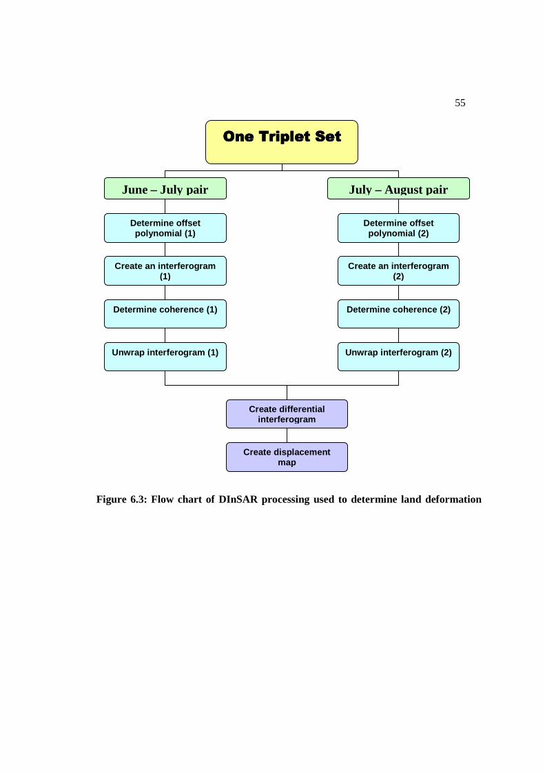
55
Figure 6.3: Flow chart of DInSAR processing used to determine land deformation
One Triplet SetOne Triplet SetOne Triplet SetOne Triplet Set
June – July pair July – August pair
Determine offset polynomial (1)
Determine offset polynomial (2)
Create an interferogram (1)
Determine coherence (2)
Create an interferogram (2)
Determine coherence (1)
Unwrap interferogram (1) Unwrap interferogram (2)
Create differential interferogram
Create displacement map

56
There were two algorithms available: the intensity cross-correlation (ICC) algorithm and
the fringe visibility (FV) algorithm. ICC was chosen for this task over FV because ICC
allows for the two images to be co-registered, even if they lack interferometric correlation
and ICC works very well with natural landscape such as the area of Reindeer Station.
The FV algorithm is computationally-time expensive and only samples a small number of
points at a time, where the ICC is much faster and can sample a user defined number of
points (must be to the power of 2). With the least squares adjustment, a test for the
highest average SNR value was run for all images and it was found that the ICC was an
average of 0.03 pixels more accurate than the FV algorithm. The decrease in accuracy
with the FV algorithm may have been a result of low a priori interferometric correlation
between the images.
Two factors, SNR and multi-looking values, were also assigned. The signal to noise ratio
(SNR) threshold was set to 7.0. This value was thought to be high enough to eliminate
any noise-induced anomalies. The average SNR values were found to be between 8.0
and 10.0, so setting 7.0 as the threshold would still include about 90% of the data. As for
the multi-looking value, it was decided to multi-look the range once and the azimuth five
times. The 1:5 range to azimuth ratio was recommended by Hanssen (2001) to yield a
square pixel. The azimuth magnitude was approximately five times the magnitude of the
range, so the azimuth was multi-looked at this point to help improve visualization of the
data and reduce azimuthal distortions. The 2:10, 3:15, 4:20 and 5:25 ratios were
attempted and it was found that the SNR value decreased linearly; therefore, the 1:5 ratio
was used.
Cropping each image to the area of interest was attempted to see if the results would be
more accurate. The hypothesis of doing this was to see if limiting the area to fewer water
bodies and less terrain differences would help improve registration accuracies. When this
was attempted using all pairs, it was found that the full images, not the cropped image,

57
provided higher accuracy in estimating the pixel offsets. The pixel offset errors of the
cropped images were caused by the software having inaccurate georeferencing within
each image.
The second step of image registration was to extract the orbit information from the
images and compute the offset of the slave image to the master image. In this step, it was
determined using tie points within the images that they were skewed in geometry and
therefore were adjusted using a simple polynomial for this transformation. Then, the
two-dimensional cross-correlation function was used to find the true relative offset by
calculating the peak correlation. The relative offset was established at this peak value.
The offset was then adjusted to subpixel accuracy using the ICC algorithm. The
algorithm uses an estimation window, size 32 by 64, to correlate the slave image to the
master image coordinates. Larger window sizes were tested as recommended by
Wegmueller et al. (2007) but they were found to lower the SNR values; therefore, the
window size of 32 pixels by 64 pixels was found to keep the highest SNR values.
Finally, once the precise offsets were established, a linear least squares polynomial was
designed to model the range and azimuth offsets. A third order polynomial was chosen to
create the best global fit and to improve the SNR of the pair. The least squares
computation removed any offsets that appeared to be in error and removed the low SNR
values; therefore creating a global fit model for the range and azimuth offset polynomials.
The accuracy obtained by the least squares estimation of less than 0.2 pixels kept the
registration errors below ten percent. The polynomial has the form of:
3
22
1
32
21
_
_
yByByBoffsetazimuth
xAxAxAoffsetrange
azimuthrangeo
azimuthrangeo
++=
++= [6.1]
58
Where Ai and Bi are the coefficients to be determined, x is the corresponding pixel
number in the range direction of the master image, and y is the corresponding pixel
number in the azimuth direction of the master image. Once the offset polynomials were
determined, the slave image was coregistered to the master image. A two-dimensional
sinc interpolator was used to resample the slave image to the master image. The
interpolator adjusted the geometry of the slave image for the best possible registration.
6.2.2 Interferogram Generation
Before the interferogram was calculated, two radiometrically calibrated intensity images
were produced from the master and slave images using the software. These two images
were overlaid as landscape references on the calculated complex images and were later
used for calculating coherence.
Then, after registering the images, the complex interferogram was generated using the
following equation:
>><<
><=*22*11
*21_
slcslcslcslc
slcslcimw [6.2]
Where * represents the complex conjugate and <> represents the ensemble average of the
complex data and the complex conjugate. This equation will calculate the wrapped
interferogram pixel by pixel. Also, in this step, a range spectral shift filter and an
azimuth common band filter were applied. The range spectral shift filter accounts for the
spectral shift due to the changes of local incidence angles between the two images. These
incidence angle changes are normally caused by the length of the baseline. The azimuth
common band filtering keeps the common frequency between the two images and rejects
the other frequencies. This filter is applied to optimize the correlation between the two
images by keeping a common band.
59
To implement the range spectral shift filter, the baselines of the image pairs had to be
calculated. The baselines were determined in range, azimuth, and altitude state vector
directions and the results were presented as a first order polynomial. The DORIS precise
orbit files allowed for accurate calculation of the baseline. This information was further
used in removal of the global phase trend and the determination of the landscape heights.
Once the baseline polynomial was known, the flat-Earth phase trend was removed. The
trend was determined by the parallel component of the baseline to the look vector of each
range swath. This trend could cause errors in the correlation function and the phase
unwrapping steps and therefore had to be removed to create a flat-Earth model.
6.2.3 Coherence Estimation
The coherence of the two images was determined by including the complex, flat-Earth
interferogram and both intensity images. A coherence estimation window of 5 pixels by
5 pixels was used to maintain the required smoothing of the complex phase information
and to enhance the accuracy of the triangular weighting scheme. It was found that
slightly larger coherence estimation windows reduced the average coherence by 0.1.
The triangular weighting scheme was calculated using a linearly decreasing value with
the increasing distance from the center pixel. Following is the coherence estimation
window weighting scheme:

60
0.057 0.255 0.333 0.255 0.057
0.255 0.529 0.667 0.529 0.255
0.333 0.667 1.000 0.667 0.333
0.255 0.529 0.667 0.529 0.255
0.057 0.255 0.333 0.255 0.057
If the coherence values were very low, there was a possibility that the branch building
step in the phase unwrapping would fail. Coherence values were not expected to be high
in all the data sets because of the quickly changing conditions of the ionosphere,
troposphere, and landscape. More information on how the coherence was affected can be
found in the results and analysis section.
6.2.4 Phase Unwrapping
Phase unwrapping a SAR image is very intensive and time-consuming. Here the branch-
cut region growing algorithm is used because of its robustness and software availability.
Because low coherence areas can be problematic by leaving discontinuities in the image,
care had to be taken when determining all parameters of the unwrapping stage. First, the
image had to be filtered and then residues and neutrons could be determined. Finally,
branches could be placed and the image could be unwrapped.
The first step of phase unwrapping is the filtering of the image. Adaptive filtering was
used to reduce phase noise and to reduce the number of residues. This low-pass filter
would self-adjust to optimize the path of the phase unwrapping branches. Then, the local
range slope was computed and the phase in the filtering window was averaged. The size
of the filtering window was 4 pixels by 4 pixels and was chosen to prevent too much
smoothing and absorb any high or low values that could contribute to noise. Also, to

61
prevent the inclusion of very low coherence values, a coherence threshold of 0.25 was
set.
Another coherence threshold flag was set after the filtering. Any areas below the defined
value of 0.1 were flagged and then a 2 pixel border surrounding the low coherence pixel
was developed. The border was used to decrease the calculation time by being able to
avoid the larger flagged areas faster than having to avoid several single pixels in one
small area. In some of the water bodies, shallow vegetation would cause the radar to
have a low coherence value and therefore attempt unwrapping, but with a threshold, this
effect could be avoided. The stray vegetation pixels within the water bodies would
increase calculation time and be ineffective for the purposes of this study. The coherence
flags were applied to the filtered image during the following phase unwrapping steps.
The first part of the actual phase unwrapping was to determine the location of the
neutrons. Neutrons are defined as areas of the interferogram where the electrical signal is
not positive or negative. The intensity of the pixel had to be at least four times the
image’s average intensity to be a valid neutron location. The neutrons helped reduce the
size of the branches and helped reduce the phase unwrapping errors; therefore reducing
the calculation time. Next, the residue locations needed to be determined. The residues
restrict the branches to stay within a particular path between locations and the “seed”
from which the branches were to grow from was set in the center of the image. The
maximum branch length was defined as 64 pixels to help prevent straying branches and
to increase computation time.
Once the image was completely encompassed by a neutral branch network, the
interferogram could be unwrapped. The unwrapping occurred only along the branches
and terminated when either the edge of the image was encountered or the branch ended.
The unwrapping began at the center of the image, in the same place as the seed and where
62
the phase was defined as zero. An example of phase unwrapping errors was in the
RADARSAT interferogram, where the unwrapped phases appear to be converging to the
center of the image (Figure 7.10). One option was to run this step multiple times to
reduce the phase unwrapping errors. Unfortunately, because the branch generation was a
two to four day process for each interferogram, this was only run once.
The final step in phase unwrapping was connecting the patches of neutral branch
networks. This process is called bridging. Phase unwrapping restarted at the end of each
bridge and finished with a difference of less than π. Bridging still considered the 2π
phase offset that may occur during the processing and adjusted the values accordingly.
6.2.5 Differential SAR Interferometry
For each triplet of images, two interferograms were produced. This allowed for the
choice to use either two pass or three pass interferometry for processing. Two pass
interferometry was attempted, but because the DEM files were a cause of errors,
technique was rejected and three pass interferometry was pursued. The software would
repeatedly return to the georeferencing default values and therefore the DEM tiles could
not be registered. It was found that three pass differential interferometry was more
successful because it did not rely on external data; therefore, it was used in determining
the vertical displacement of the topography, with a specific interest in the subsidence of
permafrost in the active delta and on the plateau. The topographic (master) interferogram
of three pass interferometry is considered to be the DEM of the area while the slave
(deformation) interferogram demonstrates the change.
In all the data sets, the June/July pair was used as the topographic pair because of the
longer baseline and the limited amount of subsidence that occurs during those months. In
63
set 3, the topographic pair did not have the longest baseline, which will have amplified
the atmospheric delay.
6.2.5.1 ENVISAT ASAR Differential Interferometry
The first step in creating a differential interferogram was to register two unwrapped
interferograms, where the slave interferogram’s baseline was larger than the master. The
baseline difference helped reduce atmospheric noise. Then, the master and slave images
were roughly registered by using a quadratic least squares algorithm to adjust for any
geometric skew or offset. The same procedure as before was used to register the
interferograms.
Once the interferograms had been coregistered, the images were differentially processed.
The phase of the slave interferogram was subtracted from the master interferogram using
a quadratic linear least squares equation (equation 19). Then using the phase information
of the differential interferogram, a metric displacement map was produced. The
displacement map in this study can display only one dimension of change because the
change in phase is over a single time period. The displacement was first determined in
the sensor’s look angle direction and then the vertical displacement was calculated. A
constant reference height of 0.00 meters was used to enhance any subsidence detected
with a precision of one centimeter.
6.2.5.2 RADARSAT Differential Interferometry
The RADARSAT images had to be processed in a different manner from the ASAR
images because only one interferogram would unwrap; and therefore the process was
slightly more complex. The offsets of the wrapped and unwrapped interferograms were

64
determined and then a new registering process was introduced. This process was very
similar to section 6.2.1, with some small modifications.
The multi-looked intensity images created in section 6.2.1 were used to determine the
slant range and azimuth offsets. Again the two-dimensional cross correlation function
was used and the peak of the function determined the offsets. This time a patch size of
1024 pixels by 1024 pixels for the correlation function was used.
To determine the sub-pixel accuracy of the co-registration, a cross-correlation
optimization was used with a window size of 64 pixels by 128 pixels. Once the precise
offsets were determined, a linear least squares polynomial was calculated to provide a
global fit of the two interferograms. Any SNR values below the threshold value of 7.0
were rejected in this calculation, therefore eliminating any blunders. Then the
interferograms were geometrically transformed using a bilinear registration function.
Finally, the two interferograms were combined to create the differential interferogram.
The final image was calculated by the following equation:
πφ 2mod)2*1*( 21 factorimagefactorimage += [6.3]
Where the factors were defined as factor1 = 1 and factor2 = -3. These values were
chosen from a series of tests where the average signal to noise ratio was found to be the
highest. The factors scale the signal noise to help determine the coherence of the final
interferogram:
2
21 21 factorfactor φφγ += [6.4]

65
The reason for dividing by the square root of 2 accounts for the statistical independence
of each original interferogram. Leaving the interferograms wrapped increases the
sensitivity to differential effects, but reduces the sensitivity to topography once they are
combined. The final steps of computing the RADARSAT differential image followed the
same process than the ENVISAT ASAR differential interferometry outlined in section
6.2.5.1.
6.2.6 Georeferencing
The images were georeferenced using ESRI ArcGIS 9.2. A Landsat 7 orthophoto of the
Reindeer Station area was acquired through GeoBase® and the major water bodies and
rivers were digitized. Using the digitized information, the differential interferogram was
then georeferenced using relative control points on the rivers and water bodies. The
RMSE of the georeferencing was 7.325 meters, approximately one pixel. A RMSE of
approximately one pixel is considered suitable because there were no absolute control
points within the images and the displacement map had poor resolution of the rivers and
water bodies.
6.3 Ground Data
6.3.1 Conventional Leveling
Ground data were acquired during the months of June and August 2005. The four
boundary corners and the center of the test site were established using static differential
GPS and steel rods. The GPS data were collected in the World Geodetic System
(WGS84) for 12 hours per point to reduce multipath effects and to improve the accuracy
of the data (Sheng et al., 2007). The internal points used to produce the DEM were

66
obtained using a Leica 1205 total station and were positioned at approximately 14 meter
intervals.
Figure 6.4: June conventional leveling data collection points
The ground data were then processed to create a surface using ordinary kriging and
polynomial trend determination using Surfer. As the August data did not work out, the
June data was used to create a digital elevation model (DEM) of the area. The DEM was
to be used to create a flow accumulation map. A hill shade and aspect map was not
considered as an option because of the northern night time sun during the summer, where
all aspects receive sunlight throughout the day. A flow accumulation map was
hypothesized to have the best qualitative assessment of the spatial structure of the
displacement map because the valley floors tend to have a higher accumulation of water;
and it is known that as more water stands on a permafrost surface, the more subsidence
will occur (Williams & Smith, 1995).
The flow accumulation map was created in ArcGIS 9.2 using the DEM created by the
conventional leveling. The georeferenced displacement map was cropped to the area of

67
interest and the flow accumulation map overlaid. The location and the structure of the
flow accumulation lines were analyzed with respect to the higher subsidence areas in the
displacement map. If the location and structure of the water accumulation matched the
higher subsidence areas, than the displacement map was considered to have acceptable
spatial accuracy.
6.3.2 Permafrost Heave Model
To determine the accuracy of the displacement map values, a permafrost heave model
created by Gugolj et al. (2008) was used. The permafrost heave model consisted of a
thermal regime model (Williams & Smith, 1989; Rankinen et al., 2004), frost front
calculations, and heave models (Konrad, 1994; Konrad, 1999). The ground
measurements were taken at 36 stations during the summer of 2005 between June 15th
and August 27th within the same test site as the conventional leveling, than it was
compared to the radar imagery.
6.3.2.1 Thermal Regime Model
The thermal regime model used in creating the permafrost heave model was a simplified
version of the finite difference function (Rankinen et al., 2004). The purpose of the
model was to calculate the daily ground temperature at one centimeter intervals using a
continuous flux. The data required for this model included soil temperature, air
temperature, snow depth, and other soil characteristics. The thermal properties of snow
were held constant because as fresh snow falls, the wind quickly changes it into a steady
state dense snow pack (Williams & Smith, 1989). The peat layer properties were not
available so they were considered to be homogenous and therefore were also held
constant.
68
The soil itself was best represented as “silty clay” and the thermal conductivity values
taken from Williams & Smith (1989). These values accounted for the variability of
thermal conductivity and heat conductivity caused by the mixture of water, ice, and soil.
The frost front was also assumed to be at the 0oC isotherm (Konrad & Morgenstern,
1981); even though the exact temperature would vary because of geological and chemical
variations (Williams & Smith, 1989).
The model would calculate the location of the 0oC isotherm within the soil on a daily
basis; then it would calculate a linear thermal gradient on either side of the frost front.
The algorithm was able to calculate dual frost fronts, as one would ascend from the
bottom of the permafrost layer and the other would descend from the surface of the soil.
6.3.2.2 Snow Distribution Model
Understanding the snow distribution is fundamental in predicting the total permafrost
coverage in the arctic. Areas with thick, continuous snow coverage tend to have limited
amounts of permafrost because snow acts as an insulator. In the test site of this study, the
snow was not continuously covering the area. To determine the snow distribution over
the test site, a geographic information system (GIS) was used. A DEM of the area was
taken and then the daily snowfall, wind magnitude, and wind direction calculated the
snow accumulation and distribution on the test site (Gugolj et al., 2008).
6.3.2.3 Heave and Subsidence Model
Other measurements, including the soil moisture and other soil properties, are used to
calculate the ice lenses influence on the heave and subsidence of the soil. The
heave/subsidence influence in the permafrost heave model is calculated as a direct

69
relation to the ice lenses’ thickness; therefore overestimating the possible subsidence
(Konrad, 1999).
The model was run for two years (2004-2005). Figure 6.5 shows the predicted elevation
changes in 2005 for the permafrost layer at the station numbered as 54. From the graph,
one can see that between June 18th and August 28th, there is a linear subsidence trend.
The linear subsidence trend during this period justified using three pass interferometry for
DInSAR and that either June/July or the July/August pair could be used as the
topographic pair, depending on the length of the baseline.
Figure 6.5: Permafrost heave model predicted elevation changes for 2005
(Gugolj, 2006)
70
CHAPTER SEVEN
RESULTS AND ANALYSIS
7.1 Data Input
The nine ENVISAT images acquired were individually processed by the European Space
Agency and the RADARSAT data was created by the Canadian Space Agency. The
RADARSAT data had the azimuth data temporally descending throughout the file;
therefore, the image had to be flipped to ensure consistency where the earliest azimuth
time is at the beginning and the range data runs from near range to far range. Table 7.1
presents the date, orbit, starting time, and size of images and Table 7.2 shows the
incidence angle and Doppler polynomial for each image.

71
Table 7.1: Raw data characteristics of images
Size (pixels) Set Date Orbit Starting
Time Rows Columns
06/18/05 17259 19:32:28 30532 5115
07/23/05 17760 19:32:28 30519 5115 1
08/27/05 18261 19:32:24 30523 5115
06/24/05 17337 06:07:21 31873 5099
07/29/05 17838 06:07:19 31875 5099 2
09/02/05 18339 06:07:15 31879 5099
06/21/05 17302 19:38:13 27478 6220
07/26/05 17803 19:38:14 27477 6220 3
08/30/05 18304 19:38:09 27482 6220
06/28/05 50365 15:28:59 11702 7695
08/15/05 51051 15:28:54 11704 7695 Radarsat
09/08/05 51394 15:28:55 11709 7695
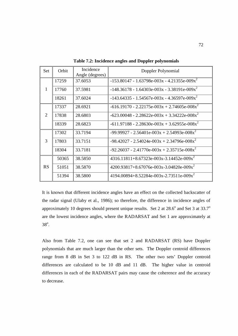
72
Table 7.2: Incidence angles and Doppler polynomials
Set Orbit Incidence Angle (degrees)
Doppler Polynomial
17259 37.6053 -153.80147 - 1.63798e-003x - 4.21355e-009x2
17760 37.5981 -148.36178 - 1.64303e-003x - 3.38191e-009x2 1
18261 37.6024 -143.64335 - 1.54567e-003x - 4.36597e-009x2
17337 28.6921 -616.19170 - 2.22175e-003x + 2.74605e-008x2
17838 28.6803 -623.00048 - 2.28622e-003x + 3.34222e-008x2 2
18339 28.6823 -611.97188 - 2.28630e-003x + 3.62955e-008x2
17302 33.7194 -99.99927 - 2.56401e-003x + 2.54993e-008x2
17803 33.7151 -98.42027 - 2.54024e-003x + 2.34796e-008x2 3
18304 33.7181 -92.26037 - 2.41770e-003x + 2.35715e-008x2
50365 38.5850 4316.11811+8.67323e-003x-3.14452e-009x2
51051 38.5870 4200.93817+8.67076e-003x-3.04820e-009x2 RS
51394 38.5800 4194.00894+8.52284e-003x-2.73511e-009x2
It is known that different incidence angles have an effect on the collected backscatter of
the radar signal (Ulaby et al., 1986); so therefore, the difference in incidence angles of
approximately 10 degrees should present unique results. Set 2 at 28.6o and Set 3 at 33.7o
are the lowest incidence angles, where the RADARSAT and Set 1 are approximately at
38o.
Also from Table 7.2, one can see that set 2 and RADARSAT (RS) have Doppler
polynomials that are much larger than the other sets. The Doppler centroid differences
range from 8 dB in Set 3 to 122 dB in RS. The other two sets’ Doppler centroid
differences are calculated to be 10 dB and 11 dB. The higher value in centroid
differences in each of the RADARSAT pairs may cause the coherence and the accuracy
to decrease.

73
7.2 Image Registration
Image registration was very successful for sets 1, 3, and RS. However, there appeared to
be problems with registering set 2. The following table shows the calculated precise
values of the offsets for each pair in each set:
Table 7.3: Range and Azimuth Offsets of Image Pairs
Pixel Size (m) Set Pair (by orbit)
Range Offset
Azimuth Offset Range Azimuth
17760 & 17259 14.400 -53.576 7.8039 15.8894 1
17760 & 18261 -24.061 -696.999 7.8039 15.8894
17838 & 17337 7.566 -62.499 7.8039 15.7207 2
17838 & 18339 -13.277 -0.269 7.8039 15.7207
17803 & 17302 6.457 2735.662 7.8039 19.5463 3
17803 & 18304 -22.875 1321.189 7.8039 19.5463
0628 & 0815 -37.385 -92.560 4.6382 25.7355 RS
0815 & 0908 -9.67306 24.87955 4.6382 25.7355
As described in section 6.2.1, a third degree quadratic least squares polynomial was
created for each pair. Higher order polynomials were attempted but they were found to
decrease the SNR; therefore being a poor representation of the offsets. The following
table presents the values of the final SNR for each pair, after all values below 7.0 dB had
been removed:
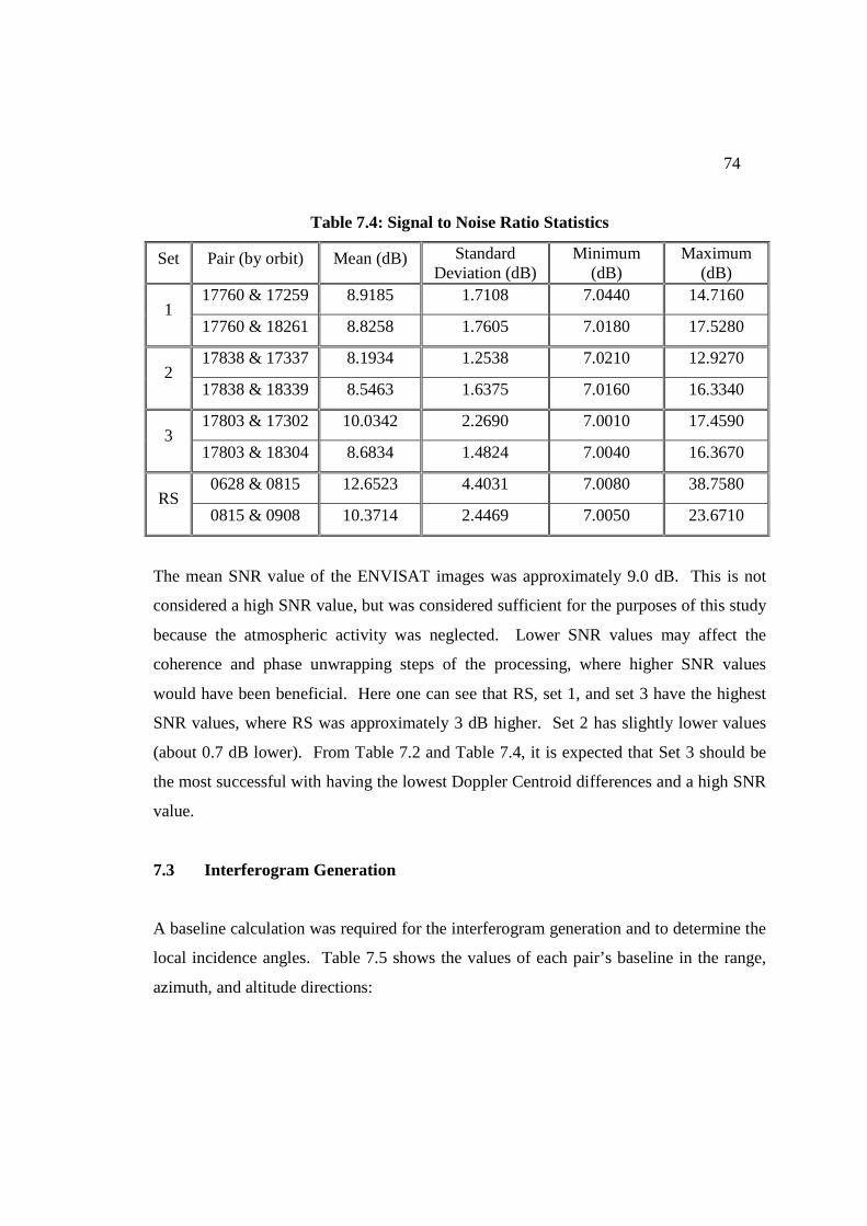
74
Table 7.4: Signal to Noise Ratio Statistics
Set Pair (by orbit) Mean (dB) Standard Deviation (dB)
Minimum (dB)
Maximum (dB)
17760 & 17259 8.9185 1.7108 7.0440 14.7160 1
17760 & 18261 8.8258 1.7605 7.0180 17.5280
17838 & 17337 8.1934 1.2538 7.0210 12.9270 2
17838 & 18339 8.5463 1.6375 7.0160 16.3340
17803 & 17302 10.0342 2.2690 7.0010 17.4590 3
17803 & 18304 8.6834 1.4824 7.0040 16.3670
0628 & 0815 12.6523 4.4031 7.0080 38.7580 RS
0815 & 0908 10.3714 2.4469 7.0050 23.6710
The mean SNR value of the ENVISAT images was approximately 9.0 dB. This is not
considered a high SNR value, but was considered sufficient for the purposes of this study
because the atmospheric activity was neglected. Lower SNR values may affect the
coherence and phase unwrapping steps of the processing, where higher SNR values
would have been beneficial. Here one can see that RS, set 1, and set 3 have the highest
SNR values, where RS was approximately 3 dB higher. Set 2 has slightly lower values
(about 0.7 dB lower). From Table 7.2 and Table 7.4, it is expected that Set 3 should be
the most successful with having the lowest Doppler Centroid differences and a high SNR
value.
7.3 Interferogram Generation
A baseline calculation was required for the interferogram generation and to determine the
local incidence angles. Table 7.5 shows the values of each pair’s baseline in the range,
azimuth, and altitude directions:

75
Table 7.5: Baselines and their breakdown
Set Pair (by orbit) Range (m) Azimuth (m) Altitude (m) Total (m)
17760 & 17259 -3.4252383 -324.9551439 66.0883528 -331.6252 1
17760 & 18261 3.1731063 299.9314535 36.5106017 302.1622
17838 & 17337 -4.3948064 -328.2697054 78.1695971 -337.4771 2
17838 & 18339 -4.1558330 241.4206063 12.6431397 241.7872
17803 & 17302 0.0002126 -217.2583308 56.3912528 -224.4575 3
17803 & 18304 0.0000049 309.0519712 41.5188001 311.8284
0628 & 0815 8.2249127 390.6051381 7.1723845 390.7575 RS
0815 & 0908 2.5033473 196.4671834 -66.5565341 207.4497
The average baseline is 293.4431 m, which is below the 500 m threshold for satellite
pairs in differential interferometry. The largest difference is approximately 183 meters
between the RS pair baselines. As the baseline difference increases, the local incidence
angle differences will increase; therefore decreasing the coherence. Also, according to
Table 7.5, the longest baselines in all sets, except set 3, were found to be in the June /
July pair. It was concluded that the June / July pairs would be used as the topographic
interferogram (i.e. the slave interferogram) to reduce the atmospheric signal delay.
7.4 Coherence Estimation
Coherence is affected by many factors and this study examines only a few of them. Any
change between acquisitions in the surrounding vegetation, water content, air humidity,
or ionosphere can reduce the coherence of an image pair dramatically. Because the
northern landscape can change abruptly, the coherence of all the pairs was not expected
to be high. If the coherence had turned out to be too low, the phase unwrapping step
should not be possible.

76
In Figure 7.1, the images of the resulting Set 1 coherence maps are overlaid on an
intensity image. The coherence threshold range was between 0.1 and 0.9. In all
subsequent coherence images, there is a linear relationship between the colour value and
the coherence value, where black is the lowest coherence and yellow is the highest.
Figure 7.1: a) 17259 & 17760 (June-July) coherence; b) 17760 & 18261 (July-
August) coherence
In these images, the dark purple represents a higher coherence than the blue. As
expected, the higher coherence was found on the plateau and the active delta has a lower
coherence with some small patches of high coherence. This result was not surprising
because of the high moisture content and high amount of vegetation in the active delta.
Table 7.6 provides the mean, standard deviation, minimum, and maximum for each
image in a high coherent area, the test site by Reindeer Station, and a low coherent area
(active delta area).
a b
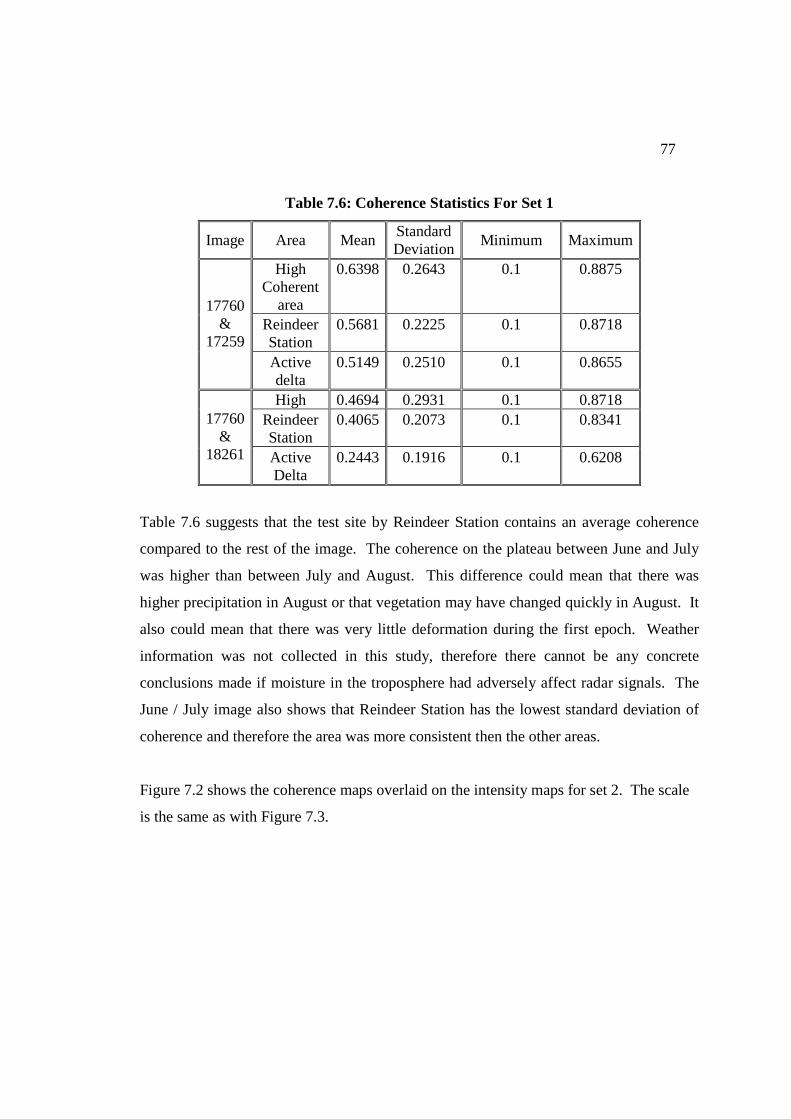
77
Table 7.6: Coherence Statistics For Set 1
Image Area Mean Standard Deviation
Minimum Maximum
High Coherent
area
0.6398 0.2643 0.1 0.8875
Reindeer Station
0.5681 0.2225 0.1 0.8718 17760
& 17259
Active delta
0.5149 0.2510 0.1 0.8655
High 0.4694 0.2931 0.1 0.8718 Reindeer Station
0.4065 0.2073 0.1 0.8341 17760 &
18261 Active Delta
0.2443 0.1916 0.1 0.6208
Table 7.6 suggests that the test site by Reindeer Station contains an average coherence
compared to the rest of the image. The coherence on the plateau between June and July
was higher than between July and August. This difference could mean that there was
higher precipitation in August or that vegetation may have changed quickly in August. It
also could mean that there was very little deformation during the first epoch. Weather
information was not collected in this study, therefore there cannot be any concrete
conclusions made if moisture in the troposphere had adversely affect radar signals. The
June / July image also shows that Reindeer Station has the lowest standard deviation of
coherence and therefore the area was more consistent then the other areas.
Figure 7.2 shows the coherence maps overlaid on the intensity maps for set 2. The scale
is the same as with Figure 7.3.

78
Figure 7.2: a) 17337 & 17838 (June-July) coherence; b) 17838 & 18339 (July-
August) coherence
Figure 7.2 shows that set 2 had very low coherence compared to set 1 (Figure 7.1). The
high coherent areas in (b) appear to be low in (a). The water bodies also appear to be not
as well defined as in set 1 or set 3 (to follow) and the images appear to be mirrored of sets
1 and 3. The poor water body definition illustrates that the lower SNR mean values that
were calculated previously may have had an ill effect on the images and because the
images are flipped in the registration step, the set 2 mirrored images suggest that the
images did not successfully register. It was hypothesized that unwrapping these images
may be very difficult. More detail on the unwrapping of these images will follow in
section 7.5. The table below shows the mean, standard deviation, minimum, and
maximum for this set.
a b

79
Table 7.7: Coherence Statistics for Set 2
Image Area Mean Standard Deviation
Minimum Maximum
Settlement 0.6438 0.2477 0.1 0.8875
Reindeer Station
0.5588 0.2212 0.2506 0.8780 17337 &
17838 Active Delta
0.5437 0.2416 0.1 0.8655
Settlement 0.6843 0.3073 0.1 0.9
Reindeer Station
0.2882 0.2007 0.1 0.6741 17337 &
18339 Active Delta
0.2230 0.1773 0.1 0.6270
Again, one can see difference in mean coherence in August. This difference again may
represent faster vegetation growth, more tropospheric moisture, or more subsidence than
in June / July.
Set 3’s coherence images are presented in Figure 7.3 with the same linear colour-
coherence relationship as the previous sets.

80
Figure 7.3: a) 17302 & 17803 (June-July) coherence; b) 17803 & 18304 (July-
August) coherence
From Figure 7.3, one can see that set 3 has low coherence in the delta with higher
coherence patches on the plateau, just as set 1 had shown. The coherence appears to
correspond between the two images better than in set 2, so unwrapping this image may be
more successful. Table 7.8 will help assist in determining this success.
b a

81
Table 7.8: Coherence Statistics for Set 3
Image Area Mean Standard Deviation
Minimum Maximum
Settlement 0.6359 0.2565 0.1 0.8875
Reindeer Station
0.5832 0.2214 0.1 0.8780 17302 &
17803 Active Delta
0.4663 0.2264 0.1 0.8623
Settlement 0.6281 0.2613 0.1 0.8875
Reindeer Station
0.5994 0.2216 0.1 0.8718 17803 &
18304 Active Delta
0.4876 0.2281 0.1 0.8623
Set 3 had the highest mean coherence values for Reindeer Station. It was concluded that
the shorter baselines of set 3 was the contributing factor in increasing the coherence
above the one for set 1.
Figure 7.4 presents the resulting coherence maps overlaid on the intensity map for the
RADARSAT sets. The threshold range is between 0.1 and 0.9 – same as the ENVISAT
images. There is also the same linear relationship between the colour value and the
coherence value, where black is the lowest coherence and yellow is the highest.

82
Figure 7.4: a) June / August coherency map; b) August / September coherency map
The RADARSAT coherence estimation appears to be similar to set 3. There are some
patches of higher coherence on the plateau in the June-August image (a), where there is
lower coherence in the same area in the August-September (b) image. The following
table provides the mean, standard deviation, minimum, and maximum for each image in a
high coherence area, the test site by Reindeer Station, and a low coherence area (active
delta area).
a
b

83
Table 7.9: Coherence Statistics for RADARSAT
Image Area Mean Standard Deviation
Minimum Maximum
Settlement 0.6158 0.2223 0.1 0.8718
Reindeer Station
0.5476 0.2180 0.1 0.8749 0628 & 0815
Active Delta
0.5392 0.2082 0.1 0.8749
Settlement 0.6133 0.2190 0.1 0.8718
Reindeer Station
0.5478 0.2219 0.1 0.8718 0815 & 0908
Active Delta
0.4910 0.2827 0.1 0.8780
The mean values for all three areas for both pairs are about 0.5, which is similar to the
ENVISAT images. The active delta values are much higher in the RADARSAT pairs
than the ENVISAT images.
Set 1 was found to have the most appropriate registration and coherence values of the
four sets because of the following reasons. Although the baselines are relatively long, the
SNR value was found to be high, the Doppler centroid differences were relatively low,
and the coherence values were suitable for proceeding with processing on the plateau.
Set 3 also showed the best coherence with the shorter baseline pair. Set 3 also displayed
a higher coherence, possibly because its SNR values were higher, the baselines were
shorter, and the Doppler centroid differences were lower.
When looking at Figures 7.1 to 7.4, one can see that set 2, set 3, and RADARSAT have
more than 50% of the landscape consisting of the active delta; where in set 1, more than
50% of the image consists of the plateau. The active delta contains a large number of
water bodies, reducing the areas of possible subsidence detection. These water bodies
may contribute to discontinuity of phase unwrapping and lead to unreliable results.

84
Therefore, although set 3 has the highest mean coherence values by approximately 0.05,
the active delta in the image may contribute to erroneous phase unwrapping.
7.5 Phase Unwrapping
Phase unwrapping is the most time-consuming, computationally-extensive process of
interferometry. Each interferogram would take up to four days to unwrap. The branch
cut algorithm allows the possibility of attempting several possible solutions for creating
branches, but because of time restraints, each interferogram was only run with one branch
solution.
Unfortunately, at the step of creating the phase unwrapping branches set 2 failed. Not
only possibly it failed because of low coherence due to registration failure, it may also
have failed because the active delta area was found in the top left hand corner of the
image and throughout the center; therefore the phase unwrapping seed was placed in a
low coherence area. Several seed locations were attempted, but they had all completed
with the same result. Also, because set 2 has the least amount of plateau land, with an
average coherence of 0.5007, and had the most active delta area, with an average
coherence of 0.2067, the branch solution would have contained a high number of
discontinuities and very small branch lengths. A divergence of the number of branches
may have caused the algorithm to fail.
Another reason as to why set 2 failed could have been because of high ionospheric
activity (Table 7.10). High geomagnetic activity can cause a relative phase shift of a
radar signal, therefore reducing coherence between two images (Hanssen, 2001). The
nearest station of recorded ionospheric activity was in Yellowknife (Geological Survey of
Canada Plotting Service), approximately 1100 km away, and one-minute readings were
used for this analysis. Sets 1 and 3 did not have any change in magnetic activity during

85
any of the acquisitions, but set 2 had a change of 25 nT between June and July and a
change of 15 nT between July and August. This change of activity could contribute to
the relative phase advancement of one of the radar signals. June and August were
attempted to be registered, where only a 10 nT change was detected, but this registration
also failed. It was concluded that the main reason for the poor registration results and
phase unwrapping failure was a combination of the low incidence angle and the
ionospheric activity.
Table 7.10: Ionospheric activity recorded in Yellowknife
Set Date of Acquisition Change in mean magnetic
activity (nano-Tesla)
1 June / July 0
July / August 0
2 June / July -25
July / August 15
3 June / July 0
July / August 0
RADARSAT June / August -3
August / September 3
See below for the unwrapped RADARSAT interferograms. These interferograms are
coloured depending on differential phase values.
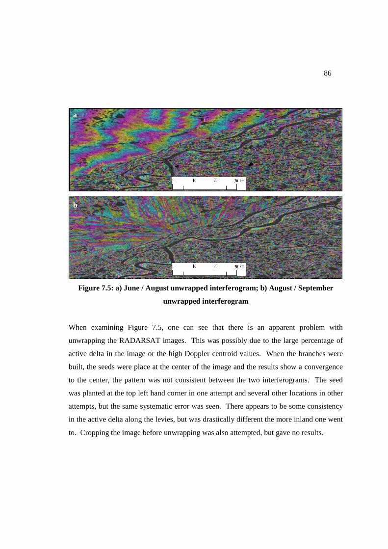
86
Figure 7.5: a) June / August unwrapped interferogram; b) August / September
unwrapped interferogram
When examining Figure 7.5, one can see that there is an apparent problem with
unwrapping the RADARSAT images. This was possibly due to the large percentage of
active delta in the image or the high Doppler centroid values. When the branches were
built, the seeds were place at the center of the image and the results show a convergence
to the center, the pattern was not consistent between the two interferograms. The seed
was planted at the top left hand corner in one attempt and several other locations in other
attempts, but the same systematic error was seen. There appears to be some consistency
in the active delta along the levies, but was drastically different the more inland one went
to. Cropping the image before unwrapping was also attempted, but gave no results.
a
b
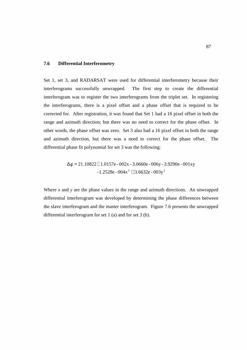
87
7.6 Differential Interferometry
Set 1, set 3, and RADARSAT were used for differential interferometry because their
interferograms successfully unwrapped. The first step to create the differential
interferogram was to register the two interferograms from the triplet set. In registering
the interferograms, there is a pixel offset and a phase offset that is required to be
corrected for. After registration, it was found that Set 1 had a 16 pixel offset in both the
range and azimuth direction; but there was no need to correct for the phase offset. In
other words, the phase offset was zero. Set 3 also had a 16 pixel offset in both the range
and azimuth direction, but there was a need to correct for the phase offset. The
differential phase fit polynomial for set 3 was the following:
22 003y-3.6632e 004x-1.2528e-
001xy-3.9290e-006y -3.0660e-002x -1.0157e21.10822
++=∆φ
Where x and y are the phase values in the range and azimuth directions. An unwrapped
differential interferogram was developed by determining the phase differences between
the slave interferogram and the master interferogram. Figure 7.6 presents the unwrapped
differential interferogram for set 1 (a) and for set 3 (b).
a

88
Figure 7.6: a) Set 1 unwrapped differential interferogram; b) Set 3 unwrapped
differential interferogram
In both images, one can see that there is disarray in the active delta. Although, in set 1
(Figure 7.6a), there are rings around the water bodies which represent the levies. The rest
of the data in the delta does not show a natural pattern of phase information, but shows a
gradual phase change towards the right (or East). A natural pattern would show pockets
of subsidence around the water bodies. The reason as to why the delta shows very little
information may be due by the high number of water bodies that caused discontinuities
along the branches in the phase unwrapping stage and therefore did not provide reliable
differential results. On the plateau, there are some gradual transforming yellow areas that
represent pockets of subsidence. A colour map to enhance the yellow areas was used and
the image was cropped to one of the pockets (Figure 7.7). In Figure 7.7, one can clearly
see the pocket of phase differences on the plateau and the phase changes along the levies.
In Figure 7.6b, set 3 did not appear to have a natural trend. It appeared that there could
be some significant subsidence, but the horizontal striping pattern of the phase difference
does not appear to contain natural pockets. Patterns similar to this could be caused by
b
a

89
atmospheric delay. As mentioned previously, a shorter baseline pair was used as the
topographic pair, which can amplify the atmospheric delay. The striping pattern could be
caused by local ionospheric or tropospheric effects. But because the ionospheric data
was not obtained for the test site and the tropospheric effects were not measured, this
could not be concluded. Also, in the active delta, one can see the levies again along the
river and water bodies, but even more disarray appears in the area. It was decided to
attempt the displacement map to see if a natural subsidence pattern would result.
Figure 7.7: Enhanced image of set 1 differential interferogram
Figure 7.8 show set 1 and set 3’s displacement maps.

90
Figure 7.8: a) Set 1 displacement map; b) Set 3 displacement map
The displacement maps were created with a colour map using the single hexagon value
index at 1 cm intervals. Positive values indicate subsidence, while negative values
indicate some upheaval. Figure 7.9 is an example of the colour map file used. The
columns of the colour map were (from left to right) vertical displacement, hue, saturation,
and intensity. B stands for background areas and F stands for forefront areas. These
areas consist of the areas that failed to unwrap. As mentioned previously, the topography
needs to be removed to create a reliable differential interferogram. It is believed that the
topography has been correctly removed from the interferograms because the subsidence
pattern on the plateau is not defined by topographic formations, such as the rolling hills.
The subsidence appears to end at the delta because of the number of water bodies and
poor phase unwrapping in that area; it is not caused by the topographic effect.
a b
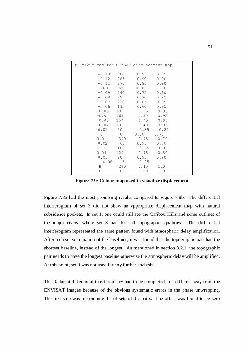
91
Figure 7.9: Colour map used to visualize displacement
Figure 7.8a had the most promising results compared to Figure 7.8b. The differential
interferogram of set 3 did not show an appropriate displacement map with natural
subsidence pockets. In set 1, one could still see the Caribou Hills and some outlines of
the major rivers, where set 3 had lost all topographic qualities. The differential
interferogram represented the same pattern found with atmospheric delay amplification.
After a close examination of the baselines, it was found that the topographic pair had the
shortest baseline, instead of the longest. As mentioned in section 3.2.1, the topographic
pair needs to have the longest baseline otherwise the atmospheric delay will be amplified.
At this point, set 3 was not used for any further analysis.
The Radarsat differential interferometry had to be completed in a different way from the
ENVISAT images because of the obvious systematic errors in the phase unwrapping.
The first step was to compute the offsets of the pairs. The offset was found to be zero
# Colour map for DInSAR displacement map
-0.13 300 0.95 0.85 -0.12 285 0.90 0.90 -0.11 270 0.85 0.90 -0.1 255 0.80 0.90 -0.09 240 0.75 0.90 -0.08 225 0.70 0.95 -0.07 210 0.65 0.95 -0.06 195 0.60 0.95 -0.05 180 0.55 0.95 -0.04 165 0.50 0.95 -0.03 150 0.95 0.95 -0.02 105 0.40 0.95 -0.01 50 0.35 0.85
0 0 0.30 0.70 0.01 300 0.95 0.70 0.02 65 0.95 0.70
0.03 180 0.95 0.80 0.04 120 0.95 0.80 0.05 20 0.95 0.90
0.06 5 0.95 1 B 290 0.45 1.0 F 0 1.00 1.0

92
using a 64 pixel by 128 pixel estimation window, but a phase fitting model was required.
The phase fitting polynomial was found to be:
2
2
003y-1.2169e-
004x-2.8762e -001xy -8.9966e 006y -1.3879e -002x -3.9302e -90.33059 ++=∆φ
The size of the estimation window allowed for the SNR to increase. The threshold of 7.0
dB was still used, therefore producing the following statistics:
Table 7.11: RADARSAT Signal to Noise Ratio Statistics
Mean (dB) Standard Deviation (dB)
Minimum (dB)
Maximum (dB)
38.4862 22.9760 7.0830 91.3290
A phase shift of approximately 90 degrees also helped enhance the SNR values. The
mean value was almost four times higher than in the original image registration, although
because of the large range of values, the standard deviation was much higher. The next
step of this process was to resample one interferogram as the slave to the master
interferogram. Then finally, the two wrapped interferograms were combined to produce
a wrapped differential interferogram (Figure 7.10) and the baselines between each pair
were determined (Table 7.12).

93
Figure 7.10: Unwrapped RADARSAT differential interferogram
Table 7.12: RADARSAT Baseline
Range (m) Azimuth (m) Altitude (m) Total (m)
-15.7349546 -198.7964121 206.8419868 287.3173
The baseline was relatively small between the two interferograms at 287 meters, but the
phase unwrapping appeared to inherit the same pattern as the unwrapped interferogram in
Figure 7.5b. This result may have occurred because of the high percentage of the active
delta in the area or because of the high Doppler centroid values. A displacement map
was created to see if a result could be recovered from the apparent error (Figure 7.11).
Figure 7.11: RADARSAT displacement map

94
The displacement map was created using the same colour map as the ENVISAT images.
The image unfortunately did not produce any results that could be corroborated with the
ground data. The displacement did not seem to correspond to any particular land mass
and only appeared at the south end of the image. It also did not follow the similar pattern
than the other two sets that used unwrapped interferograms. The possible reason for this
result could be attributed to the high Doppler centroid differences found in the pair of
interferograms or atmospheric effects. Therefore, the RADARSAT images were not
analyzed any further, but were used as an example of high Doppler centroid differences.
To enhance the displacement of set 1, a new colour map was used and then the image was
georeferenced (Figure 7.12). There was subsidence of up to 6 cm found on the plateau,
but areas of missing information could also be seen. These areas include the delta and
the northern part of the plateau. It was concluded that the reason behind the missing
information was because of the higher number of present water bodies causing phase
unwrapping discontinuities. The new subsidence map was then cropped down to the test
site by Reindeer Station (Figure 7.12) so a comparison could be completed.

95
Figure 7.12: Displacement map of set 1 where blue shows zero subsidence and
brown shows 6 cm of subsidence and an enlargement of the area of interest
7.7 Ground Data Correlation
As mentioned in section 6.3.1, an attempt was made to compare the land structure of the
test site using a flow accumulation map. Figure 7.13 shows the flow accumulation map
(the bright red lines) laid over the interferogram of the test site. It was impressive to see
how well the accumulation map corresponded with the interferogram. Similar structures
in both maps, such as the U shape area near the center of the image, were found to relate
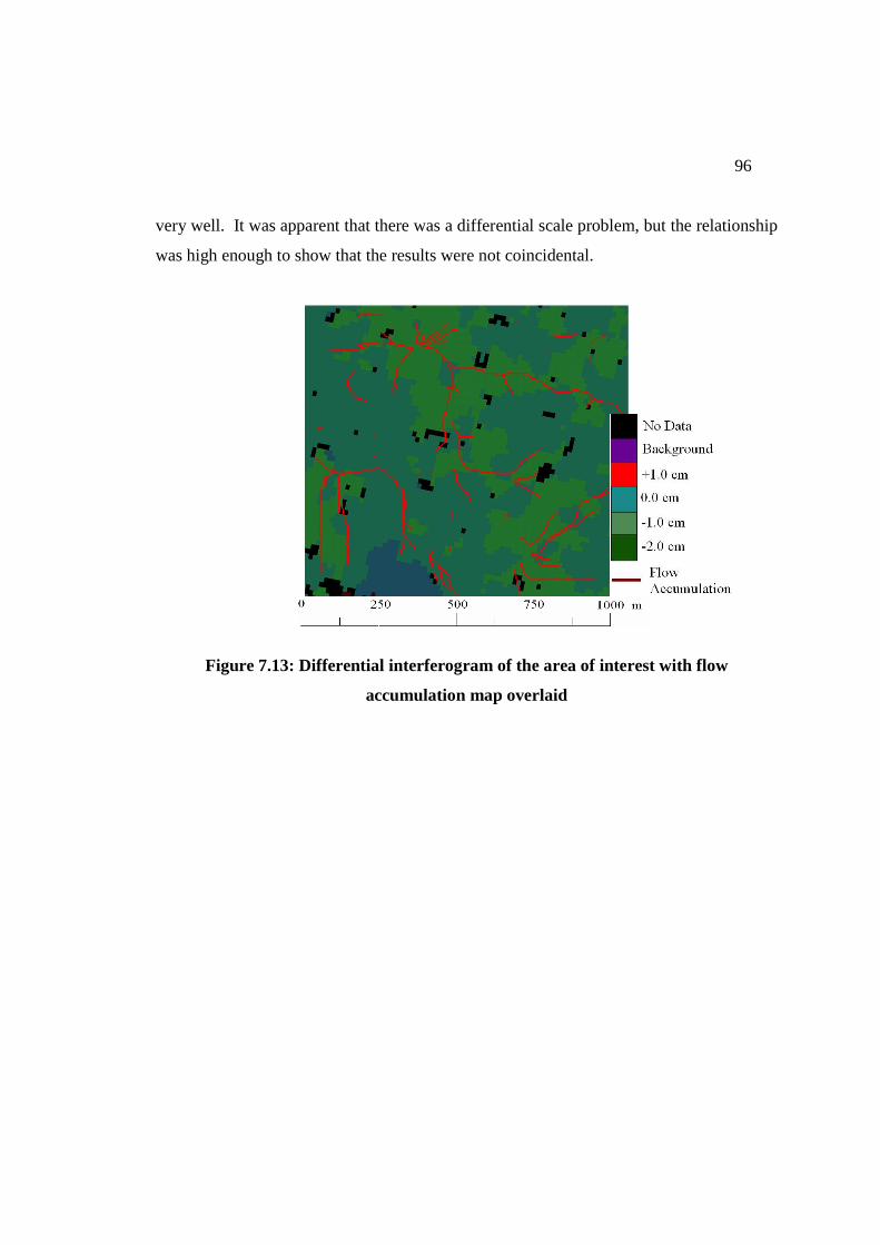
96
very well. It was apparent that there was a differential scale problem, but the relationship
was high enough to show that the results were not coincidental.
Figure 7.13: Differential interferogram of the area of interest with flow
accumulation map overlaid

97
Figure 7.14: Displacement map compared with the permafrost heave model
Because the flow accumulation map of the DEM attested to the structural composition of
the interferogram, the next important comparison was to ensure that the magnitude of the
interferogram was also correct. Subsidence of up to 2 cm can be seen in Figure 7.14,
where the permafrost heave model shows a subsidence of up to 3 cm, with an average of
1.9 cm +- 1.5 cm, during the months of June through August. The correlation of the
magnitude was also remarkable in this case. The differences in magnitude could be
attributed to the fact that DInSAR averaged the scattering response over a large area (7 m
by 15 m), where the heave model was a discrete point.
- 1.5±0.5
- 2.5±0.5

98
CHAPTER EIGHT
CONCLUSIONS AND RECOMMENDATIONS
8.1 Conclusions
This study is a preliminary study of the use of DInSAR in monitoring permafrost
subsidence. Promising results have been found in one of the four sets and therefore
additional work and research is still required to develop more concrete conclusions.
From the analysis of Set 1, it was found that there was an intraseasonal subsidence up to
6 cm on the plateau and 3 cm subsidence in the area of interest between June 18th and
August 27th, which appears reasonable when compared to the permafrost heave model.
There was a lack of information in the active delta and in the northwest section of the
image. This deficiency was possibly created by the problems with the branch cut phase
unwrapping algorithm.
Four displacement maps were created with centimeter accuracy. After processing and
analyzing these image sets, it became apparent that ENVISAT set 1 was the only data set
that appeared to process correctly. Set 1 was found to have shorter baselines, a higher
SNR, similar Doppler centroid differences, and similar ionospheric activity values than
Set 3. The possible reason for the result differences is that Set 1 had the higher incidence
angle and that the baseline correction may have caused an amplified atmospheric effect.
Set 2 had unsuccessful geometric registration and the reason for this was thought to be
from the lowest incidence angle and higher ionospheric activity. RADARSAT had the
shortest baseline and the highest SNR, but was found to provide incorrect results. It is
believed that the poor results were because of the large Doppler centroid change (122dB)
in one of the pairs.

99
The most prominent factor that appeared to affect the results was the phase unwrapping
algorithm. It appears that the branch cut algorithm had difficulties unwrapping the
images because of the number of water bodies and the relatively low coherence. When
creating the branch network, the algorithm appears to have a diverging number of
branches, causing it to crash or provide poor results.
From the other image sets that did not process correctly, it could be concluded that
possibly the extent of high coherence areas in an image greatly affects the ability to
provide results. The number of discontinuities in the phase cycles greatly increases when
there is a high number of water bodies.
As Ulaby et al. had reported in 1986, the incidence angle also had an effect on the
processed image quality. Set 1 had an incidence angle of 37.5 degrees and was the only
data set that works properly. The optimal incidence angle in the arctic on plateau land
may be around 37 degrees as RADARSAT did not work at 38.5 degrees and set 3 did not
work at 33.7 degrees.
The environmental, atmospheric, tropospheric, and ionospheric changes could have also
affected the radar signal and therefore providing biased results. As in Set 2, the
geomagnetic differences at the time of capture in the ionosphere were found to be the
highest and it was the first image to show poor results. Environmental, atmospheric, and
tropospheric changes were not taken into account. These changes may have also affected
the sets and may have attributed to a possible bias of the results of Set 1 and therefore
creating inaccurate values. Another factor that appeared to affect the images was the
Doppler centroid differences. The data sets with the high Doppler polynomial values also
processed incorrectly.

100
Finding enough similar images to create a high redundancy of data was found to be very
difficult in this line of work. Environmental changes happen quickly and with the local
incidence angle changes, Doppler centroid differences, and atmospheric effects, it can be
difficult to determine one factor affecting the results of the radar signal. Isolating each
independent variable requires more data than just four sets of images.
At the conclusion of this study, only one displacement was successfully created. This
map may not be completely accurate as there were several factors that were not taken into
consideration – such as the tropospheric and local ionospheric data – but it was found that
the results did correspond well with ground data.
Relating the interferogram with the aspect map of digital elevation model created by
conventional surveying was attempted but was found to be inaccurate. The inaccuracy
was caused by the 24 hour sun the area has during the summer; therefore the aspects
covered a 360o circle. But when a flow accumulation map was created with the same
model, a good correspondence was found with the valley floors and higher areas of
subsidence.
A correspondence was found between the interferogram and the permafrost heave model.
The heave model used point data locations within the area of interest and these points
corresponded very well with the interferogram. The differences seen are possibly
because the information found in the pixels in the interferogram is averaged over a large
area while the permafrost heave model is point data.
In conclusion, a deformation map was created for an area of 1500 km2 on plateau land
and the same processing method could be used for other plateaus that consist of 7% of the
northern landscape. It was found that the incidence angle, Doppler centroid differences,
and phase unwrapping algorithms may be the cause of error in completing this work.

101
Because of the lack of redundancy, no results can be guaranteed. With additional work
and research, DInSAR could be used to monitor annual changes and monitor the effect of
climate change on permafrost in a more cost effective manner.
8.2 Recommendations
This project still requires more research, processing, and ground work to be more
conclusive. The following points are suggestions for future research.
- More research into the number of triplets required should be completed.
Redundancy is difficult to obtain in the arctic because of the effects of
geometric and environmental parameters and their numerous possibilities.
- The effect of the incidence angle on DInSAR in this area should be further
researched. Previously, Bamler & Hartl (1998) had recommended an
incidence angle of 45o for DInSAR, but in this study the highest incidence
angle was 38o. More images should be acquired with different incidence
angles to determine the optimal angle.
- Several factors can affect the quality of the results and three of these factors
were not accounted for – environmental, tropospheric, and ionospheric. A
scatterometer could be used to help determine dielectric constants of the
changing surface vegetation and perhaps develop a new way to increase
coherence. To account for ionospheric and tropospheric effects, differential
global positioning systems could be used to gather the information and then
implemented in the processing of the radar images.
102
- Doppler centroid differences also played an important role in affecting the
interferogram results. These differences should also be tested in the future to
determine if the Doppler values truly affect differential interferometry results
in northern environments.
- Timing of the acquisitions is also important. For example, when the snow
first disappears off the surface, it is predicted by the permafrost heave model
that the greatest amount of subsidence occurs. When gathering the radar
images, it would be important to acquire more imagery around this time so a
more accurate conclusion of yearly subsidence can be made.

103
REFERENCES
Abdelfattah, R. and Nicola, J. 2003. InSAR Coherence Optimisation using Second Kind
Statistics, IGARSS 6: 3799-3801.
Allard, M., and Rousseau, L. 1999. The internal structure of a palsa and a peat plateau in
the rivie`re Boniface region, Que´bec: Inferences on the formation of ice segregation
mounds, Geogr. Phys. Quat. 53: 373–387.
Anderson, C. 1995. Fringe visibility, irradiance, and accuracy in common path
interferometers for visualization of phase disturbances, Applied Optics 34(32): 7474-
7485.
Anisimov, O. and Belolutskaya, M. 2002. Evaluation of the effect of climate change and
permafrost degradation on infrastructure in the northern regions of Russia, Russian
Meteorology and Hydrology 6: 9-14.
Anisimov, O. and Poliakov, V. 2003. GIS assessment of climate-change impacts in
permafrost regions, 8th International Conference on Permafrost, Balkema: Zurich; 9–14.
Annan, A. and Davis, J. 1978. High frequency electrical methods in the detection of the
freeze–thaw interface, Third International Conference on Permafrost 1: 495–500.
Bamler, R. 1992. A comparison of range-Doppler and wave number domain SAR
focusing algorithms, IEEE Transactions of Geoscience and Remote Sensing 30(4): 706-
713.

104
Bamler, R. and Hartl, P. 1998. Synthetic aperture radar interferometry, Inverse Problems
14(4): R1-R54.
Bamler, R. and Just, D. 1993. Phase statistics and decorrelation in SAR interferograms,
IGARSS 3: 985-987.
Barsch, D. 1993. Periglacial geomorphology in the 21st century, Geomorphology 7: 141–
163.
Beltrami, H. and Taylor, A. 1994. Records of climatic change in the Canadian Arctic:
combination of geothermal and oxygen isotope data yields high resolution ground
temperature histories. EOS, Transactions, American Geophysical Union 57(44): 75.
Billings, W. 1987. Constraints to plant growth, reproduction, and establishment in Arctic
environments, Arctic & Alpine Research 19(4): 357-365.
Bracewell, R. 1986. The Fourier transform and its applications, McGraw-Hill, New
York. 3rd edn.
Brown, J., Hinkel, K.M., and Nelson, F.E. 2000. The Circumpolar Active Layer
Monitoring (CALM) Program: Research Designs and Initial Results, Polar Geography
24(3): 165-258.
Burgess, M., Smith, S.L., Brown, J., Romanovsky, V., Hinkel, K. 2000. Global
Terrestrial Network for Permafrost (GTN-P): permafrost monitoring contributing to
global climate observations. Geological Survey of Canada, 1 –8 (Current Research
2000-E14).

105
Butterworth, C. and Tait, M. 2007. Monitoring Permafrost Deformation, Proc.
International Circumpolar Conference on Geospatial Sciences and Applications (CD).
CALM Site Homepage. 2006. Available at: http://www.udel.edu/Geography/calm/
Canadian Geographic. 2008. The Far North: Arctic and Taiga. The Canadian Atlas
Online, Available at: http://www.canadiangeographic.ca/atlas/themes.aspx?id=artic
&lang=En
Carnec, C. and Delacourt, C. 2000. Three years of mining subsidence monitored by SAR
interferometry, near Gardanne, France, Journal of Applied Geophysics 43(1): 43-54.
Couture, R., Smith, S., Robinson, S., Burgess, M., and Solomon, S. 2003. On the hazards
to infrastructure in the Canadian North associated with thawing of permafrost,
Geohazards 2003, 3rd Canadian Conference on Geotechnique and Natural Hazards. The
Canadian Geotechnical Society: Edmonton, Alberta, Canada; 97–104.
Cramer, M., Ferland, R., and Snay, R. 1999. Realization and unification of NAD83 in
Canada and the U.S. via the ITRF, International Symposium of the International
Association of Geodesy 2, Munich, October 5-9.
Crippa, B., Crosetta, M., Biescas, E., Troise, C., Pinque, R., and De Natale, G. 2006. An
advanced slip model for the Umbria-Marche earthquake sequence: coseismic
displacements observed by SAR interferometry and model inversion, Geophys. J. Int. 164
(1): 36–45.
Cumming, I. and Wong, F. 2005. Digital processing of Synthetic Aperture Radar Data –
Algorithms and Implementation. Artech House, Inc., Norwood, MA.

106
Cusack, R., Huntley, J., and Goldrein, H. 1995 Improved noise immune phase
unwrapping algorithm, Applied Optics 35, 781–789.
Davis, T. 2001. Permafrost: a Guide to Frozen Ground in Transition. University of
Alaska Press: Fairbanks.
Denbigh, P. 1995. System Analysis and Signal Processing with Emphasis on the Use of
Matlab, Addison-Wesley, Boston, MA.
Dionne, J. 1978. Formes et phe´nome`nes pe´riglaciaires en Jame´sie, Que´bec
subarctique, Geogr. Phys. Quat. 32: 187– 247.
Doolittle, J., Hardisky, M., and Gross, M. 1990. A ground penetrating radar study of
active layer thicknesses in areas of moist sedge and wet sedge tundra near Bethel,
Alaska,U.S.A. Arctic and Alpine Research 22: 175–182.
Doolittle, J., Hardisky, M., and Black, S. 1992. A ground penetrating radar study of
Goodream Palsen, Newfoundland, Canada, Arctic and Alpine Research 24: 173–178.
Eldhuset, K., Andersen, P., Hauge, S., Isaksson, E. and Waydahl, D. 2003. ERS tandem
InSAR processing for DEM generation, glacier motion estimation and coherence analysis
on Svalbard, Int. J. Remote Sens. 24(7): 1415-1437.
European Space Agency. 2006. ASAR Products and Algorithms. Available online at:
http://envisat.esa.int/dataproducts/asar/CNTR2-6.htm
107
Fialko, Y., Sandwell, D., Simons, M., and Rosen, P. 2005. Three dimensional
deformation caused by the Bam, Iran, earthquake and the origin of shallow slip deficit,
Nature 435, 295-299.
Fielding, K. and Dupre, E. 1999. RNGCHN: A program to calculate displacement
components from dislocations in an elastic half-space with applications for modeling
geodetic measurements of crustal deformation, Geophysical Research Letters 25: 695 –
704.
Flato, G., Boer, G., Lee, W., McFarlane, N., Ramsden, D., Reader, M., and Weaver, A.
2000. The Canadian Centre for Modelling and Analysis Global Coupled Model and its
climate, Climate Dynamics 16: 451–467.
Foody, G. and Curran, P. 1994. Environmental Remote Sensing from Regional to Global
Scales, John Wiley & Sons, Chichester, England, pp. 8-10, 202-207.
French, H. 1996. The Periglacial Environment. Addison Wesley Longman: London, UK.
Gabriel, A., Goldstein, R., and Zebker, H. 1989. Mapping small elevation changes over
large areas: differential radar interferometry, Journal of Geophysical Research 94(B7):
9183 – 9191.
Ghiglia, D. and Pritt, M. 1998. Two Dimensional Phase Unwrapping: Theory,
Algorithms, and Software. John Wiley & Sons Inc.
Goldstein, R. 1995. Atmospheric limitations to repeat-track radar interferometry, J.
Geophys. Res. 22: 2517–2520.
108
Goldstein R. and Zebker, H. 1987. Interferometric radar measurement of ocean surface
currents, Nature 328(6132): 707-709.
Goldstein, R., Zebker, H., and Werner, C. 1988. Satellite radar interferometry: two
dimensional phase unwrapping, Radio Sci. 23, 713–720.
Graham, L. 1974. Synthetic interferometer radar for topographic mapping, Proc. IEEE
62(6): 763-768.
Granberg, H. 1994. Mapping heat loss zones for permafrost prediction at the
northern/alpine limit of the Boreal forest using high-resolution C-Band SAR, Remote
Sens. Environ. 50(3), 280-286.
Gray, A., Mattar, K., and Sofko, G. 2000. Influence of Ionospheric Electron Density
Fluctuations on Satellite Radar Interferometry, Geophysical Research letters 27(10):
1451-1454.
Gruza, G. and Rankova, E. 1980. Structure and Variability of the Observed Climate. Air
Temperature in the Northern Hemisphere. Gidrometeoizdat, Leningrad.
Guglielmin, M. 2006. Ground Surface Temperature (GST), Active Layer and
Permafrost Monitoring in Continental Antarctica, Permafrost and Periglac. Process. 17:
133–143.
Guglielmin, M. and Dramis, F. 1999. Permafrost as a climatic indicator in northern
Victoria Land, Antarctica, Annals of Glaciology 29: 131–135.
109
Gugolj, D. 2006. Permafrost Active Layer Motion Modeling: A Geographic Information
Systems (GIS) Approach, MGIS Project, Department of Geography, University of
Calgary.
Gugolj, D., Moorman, B., and Tait, M. 2008. Development and Initial Evaluation of a
Daily DEM-Based Active Layer Heave and Subsidence Model, Ninth International
Conference on Permafrost, June 29 – July 3.
Gutmann, B. and Weber, H. 2000. Phase unwrapping with the branch-cut method: role of
phase-field direction, Applied Optics 39(26): 4802-4816.
Haeberli, W., Cheng Guodong, Gorbunov, A., and Harris, S. 1993. Mountain Permafrost
and Climate Change, Permafrost and Periglacial Processes 4(2): 165 – 174.
Hall-Atkinson, C. and Smith, L. 2001. Delineation of delta ecozones using
interferometric SAR phase coherence Mackenzie River Delta, N.W.T., Canada, Remote
Sens. Environ. 78: 229– 238.
Hanssen, R. 2001. Radar Interferometry: Data Interpretation and Error Analysis.
Kluwer Academic Publishers.
Hanssen, R. 2006. Temporal Decorrelation. Available online:
http://earth.esa.int/workshops/ers97/papers/hanssen/node7.html
Hanssen, R. and Feigt, A. 1996. A first quantitative evaluation of atmospheric effects on
SAR interferometry, FRINGE 96’ workshop on ERS SAR Interferometry ESA SP – 406:
277 - 282.

110
Harris, C., Vonder Mühll, D., Isaksen, K., Haeberli, W., Sollid, J., King, L., Holmlund,
P., Dramis, F., Guglielmin, M., and Palacios, D. 2003. Warming permafrost in European
mountains, Global and Planetary Change 39: 215–225.
Hauck, C. and Vonder Mühll, D. 2003. Evaluation of geophysical techniques for
application in mountain permafrost studies, Geophysical methods in geomorphology 132:
161–190.
Heginbottom, J. 1973. Some effects of surface disturbance on the permafrost active layer
at Inuvik, N.W.T., Canada, 2nd International Permafrost Conference North American
Contribution : 649-657.
Hein, A. 2004. Processing of SAR Data. Springer, New York.
Hinkel, K., Paetzold, F., Nelson, F., and Bockheim, J. 2001a. Patterns of soil temperature
and moisture in the active layer and upper permafrost at Barrow, Alaska: 1993–1999,
Global and Planetary Change 29: 293–309.
Hinkel, K., Doolittle, J., Bockheim, J., Nelson, F., Paetzold, R., Kimble, J., and Travis, R.
2001b. Detection of Subsurface Permafrost Features with Ground-Penetrating Radar,
Barrow, Alaska, Permafrost Periglac. Process. 12: 179–190.
Ishikawa, M. 2003. Thermal regimes at the snow–ground interface and their implications
for permafrost investigations, Geomorphology 52:105–120.
Ishikawa, M., Watanabe, T. and Nakamura, N. 2001. Genetic difference or rock glaciers
and the discontinuous mountain permafrost zone in Kanchanjunga Himal, eastern Nepal,
Permafrost and Periglacial Processes 12: 243–253.
111
Janke, J. 2005. Modeling past and future alpine permafrost distribution in the Colorado
Front Range, Earth Surface Processes and Landforms 30: 1495–1508.
Jorgenson, M., Racine, C., Walters, J., and Osterkamp, T. 2001. Permafrost degradation
and ecological changes associated with a warming climate in central Alaska. Climatic
Change 48: 551–579.
Kakunov, N. 1999. Monitoring of the active/seasonally frozen layer and upper layers of
cryolithozone during the ongoing half-century climatic cycle in the European northeast of
Russia, Abstracts of the International Conference ‘Monitoring of Cryosphere’
(Pushchino, Russia, 20–23 April 1999), 120–121.
Kneisel, C. 2006. Assessment of subsurface lithology in mountain environments using
2D resistivity imaging, Geomorphology 80: 32–44.
Kneisel, C. and Hauck, C. 2003. Multi-method geophysical investigation
of a sporadic permafrost occurrence, Geophysical methods in geomorphology 132: 145–
159.
Kneisel, C., Saemundsson, P., and Beylich A. 2007. Reconnaissance surveys of
contemporary permafrost environments in central Iceland using geoelectrical methods:
implications for permafrost degradation and sediment, Geogr. Ann. 89 A (1): 41–50.
Knopfle, W. 1999. Visualization of interferometric products derived from ERS1/2
tandom pair data, IGARSS 2: 1378-1380.
112
Komarov, S., Mironov, V., and Li, S. 2002. SAR polarimetry for permafrost active layer
freeze/thaw processes, IGARSS: 2654-2656.
Konrad, J.M. 1994. Sixteenth Canadian Geotechnical Colloquium: Frost heave in soils:
concepts and engineering, Canadian Geotechnical Journal, 31: 223-245.
Konrad, J.M. 1999. Frost susceptibility related to soil index properties, Canadian
Geotechnical Journal, 36: 403-417.
Krautblatter, M. and Hauck, C. 2007. Electrical resistivity tomography monitoring of
permafrost in solid rock walls, J. Geophys. Res. 112, F02S20,
Laberge, M. and Payette, S. 1995. Long-Term Monitoring of Permafrost Change in a
Palsa Peatland in Northern Quebec, Canada: 1983-1993, Arctic and Alpine Research
27(2): 167-171.
Lachenbruch, A. and Marshall, B. 1986. Changing climate: geothermal evidence from
permafrost in the Alaskan Arctic. Science 234: 689–696.
Lanari, R., Fornaro, G., Riccio, D., Migliaccio, M., Papathanassiou, K., Moreira, J.,
Schwabisch, M., Dutra, L., Puglisi, G., Franceschetti, G., and Coltelli, M. 1996.
Generation of digital elevation models by using SIR-C/X-SAR multifrequency two-pass
interferometry: the Etna case study, IEEE Transactions on Geoscience and Remote
Sensing 34(5): 1097-1114.
Laprise, D. and Payette, S. 1988. Evolution recente d’une tourbiere apalses (Quebec
subarctique): Analyse cartographique et dendrochronologique, Can. J. Bot. 66: 2217–
2227.

113
Li, F. and Goldstein, R. 1990. Studies of multibaseline spaceborne interferometric
synthetic aperture radars, IEEE Trans. GE-28(1), pp 88-98.
Li, Z., Li, X., Ren, X. and Dong, Q. 2003. Frozen ground deformation monitoring using
SAR interferometry, Proc. IEEE 4: 2933 – 2935.
Little, J., Sandall, S., Walegur, M., and Nelson, F. 2003. Application of differential
global positioning systems to monitor frost heave and thaw settlement in tundra
environments, Permafrost Periglac. 14: 349-357.
Lu, Z. and Freymueller, J. 1998. Synthetic aperture radar interferometry coherence
analysis over Katmai volcano group, Alaska, J. Geophys. Res. 103: 29,887–29,894.
Lu, Z., Power, J., McConnell, V., Wicks, C. and Dzurisin, D. 2002. Preeruptive inflation
and surface interferometric coherence characteristics revealed by satellite radar
interferometry at Makushin Volcano, Alaska: 1993–2000, J. Geophys. Res. 107(B11),
ECV 1 1-13.
Mackay, J., Ostrick, J., Lewis, C., Mackay, D. 1979. Frost heave at ground temperatures
below 0 8C, Inuvik, Northwest Territories, Paper-Geological Survey of Canada 79-1A:
403–406.
Massonnet, D. and Feigl, K. 1995a. Satellite radar interferometric map of the coseismic
deformation field of the M = 6:1 Eureka Valley California earthquake of May 17, 1993,
Geophys. Res. Lett. 22: 1541–1544.

114
Massonnet, D. and Feigl, K. 1995b. Discrimination of geophysical phenomena in satellite
radar interferograms, Geophys. Res. Lett. 22: 1537–1540.
Mauro, G. 2004. Observations on permafrost ground thermal regimes from Antarctica
and the Italian Alps, and their relevance to global climate change. Global and Planetary
Change 40: 159–167.
Maxwell, B. 1997. Responding to global climate change in Canada’s Arctic, Volume II
of the Canada Country Study: Climate impacts and adaptation. Environment Canada.
Merry, C. 1998. Basics of Levelling. Lecture Series – University of Cape Town.
Available at: http://64.233.167.104/search?q=cache:CPjeuX-
qsCYJ:www.pol.ac.uk/psmsl/training/levelling.doc+Precise+levelling&hl=en&gl=ca&ct
=clnk&cd=4
Miller, L., Hinkel, K., Nelson, F., Paetzold, R., Outcalt, S. 1998. Spatial and temporal
patterns of soil moisture and thaw depth at Barrow, Alaska U.S.A. Permafrost-Seventh
International Conference Universite Laval Centre d’etudes nordiques, Quebec, Canada,
pp. 731–737.
Mironov, V., Komarov, S., Li, S., and Romanovsky, V. 2005. Freeze-thaw processes
radar remote sensing: modeling and image processing. IGARSS: 608-611.
Moldoveanu, M., Stewart, R., Aitken, J., and Gallant, E. 2003. 3D Ground Penetrating
Radar over ice and Permafrost, CSEG. Available at: www.crewes.org/Conference-
abstracts/2003/SEG/Moldoveanu_SEG_2003.pdf
115
Moorman, B. and Vachon, P. 1998. Detecting ground ice melt with interferometric
synthetic aperture radar, 20th Canadian Symposium on Remote Sensing, Calgary, Alberta,
May 10-13.
Muellerschoen, R., Chen, C., Hensley, S., and Rodriguez, E. 2006. Error Analysis for
High Resolution Topography with Bi-static Single-Pass SAR Interferometry, IEEE
Conference on Radar 8: 626 – 633.
National Center for Atmospheric Research. 2005. Most Of Arctic's Near-surface
Permafrost To Thaw By 2100, ScienceDaily. Retrieved January 20, 2008, from
http://www.sciencedaily.com /releases/2005/12/051220085054.htm
Nelson, F. and Anisimov, O. 1993. Permafrost zonation in Russia under anthropogenic
climate change, Permafrost and Periglacial Processes 4(2): 137-148.
Nelson, F., Hinkel, K., Shiklomanov, N., Mueller, G., Miller, L., Walker, D. 1998a.
Active-layer thickness in north-central Alaska: systematic sampling, scale, and spatial
autocorrelation, Journal of Geophysical Research-Atmospheres 103 (22): 28963–28973.
Nelson, F., Outcalt, S., Brown, J., Shiklomanov, N., and Hinkel, K. 1998b. Spatial
temporal attributes of the active-layer thickness record, Barrow, Alaska, USA, 7th
International Conference on Permafrost, Yellowknife, Canada. Centre d’e´tudes
nordiques, Universite´ Laval, pp. 797– 802.
Nelson, F., Mueller, G., and Shiklomanov, N. 1999. Variability of active-layer thickness
at multiple spatial scales, north-central Alaska, U.S.A. Arctic, Antarctic, and Alpine
Research 31 (2): 158–165.
116
Nelson, F., Anisimov, O., and Shiklomanov, N. 2002. Climate Change and Hazard
Zonation in the circum-arctic permafrost regions, Natural Hazards 26(3): 203-225.
Nelson, F. and Hinkel, K. 2003. Methods for Measuring Active-Layer Thickness.
Available at: www.unis.no/RESEARCH/GEOLOGY/Geo_research/Ole/Periglacial
Handbook/ActiveLayerThicknessMethods.htm
Nelson, F., Lachenbruch, A., Woo, M., Koster, E., Osterkamp, T., Gavrilova, M., and
Cheng, G. 1993. Permafrost and Change Climate, 6th International Conference on
Permafrost 2: 987-1005.
Nixon, F. and Taylor, A. 1998. Regional active layer monitoring across the sporadic,
discontinuous and continuous permafrost zones, Mackenzie valley, northwestern Canada.
7th International Conference on Permafrost, Yellowknife, Canada, pp. 815– 820.
Oberman, M. and Mazhitova, G. 2001. Permafrost dynamics in the north-east of
European Russia at the end of the 20th century, Norsk Geografisk Tidsskrift - Norwegian
Journal of Geography 55:4, 241 – 244.
Osterkamp, T., Zhang, T. and Romanovsky, V. 1994. Evidence for a cyclic variation of
permafrost temperature in northern Alaska, Permafrost and Periglacial Processes 5:
137–144.
Ottesen, J., Galligan, D., Sterley, D., Burden, P., Wong, B., and Aho, J. 2002. An
examination of resource transportation alternatives in Northwest Alaska, Cold Regions
Engineering Cold Regions Impacts on Transportation and Infrastructure: Proceedings of
the Eleventh International Conference p.182-193.

117
Pavlov, A. 1994. Current changes of climate and permafrost in the Arctic and sub-Arctic
of Russia, Permafrost & Periglacial Processes 5(2): 101-110.
Payette, S., Delwaide, A., Caccianiga, M., and Beauchemin, M. 2004. Accelerated
thawing of subarctic peatland permafrost over the last 50 years, Geophys. Res. Lett. 31:
L18208.
Pilon, J., Annan, A., Davis, J., and Gray, J. 1979. Comparison of thermal and radar active
layer measurements in the Leaf Bay Area, Nouveau-Quebec, Geographie Physique et
Quaternaire 23: 317–326.
Pilon, J., Annan, A., and Davis, J. 1985. Monitoring permafrost ground conditions with
ground probing radar (G.P.R.), Workshop on Permafrost Geophysics, Golden, Colorado,
CRREL Special Report 85-5: 71–73.
Rankinen, K., Karvonen, T., and Butterfield, D. 2004. A simple model for predicting soil
temperature in snow-covered and seasonally frozen soil: Model description and testing,
Hydrology and Earth System Sciences, 8(4): 706-716.
Rao, Y., Venkataraman, G., Rao, K., and Snehmani. 2004. SAR interferometry for DEM
generation and movement of Indian glaciers, IGARSS 2: 1128-1131.
Rodiguez, E. and Martin, J. 1992. Theory and design of interferometric synthetic
aperture radars, Pro. IEEE -F 139(2): 147-159.
Romanovsky, V., Burgess, M., Smith, S., Yoshikawa, K., and Brown, J. 2002. Permafrost
temperature records: indicators of climate change. EOS, Transactions of the American
Geophysical Union 83: 589, 593–594.

118
Rosen, P., Hensley, S., Zebker, H., Webb, F., and Fielding E. 1996. Surface deformation
and coherence measurements of Kilauea volcano, Hawaii from SIR-C radar
interferometry, Journal of Geophysical Research 101(E10): 23109-23135.
Rosen, P., Hensley, S., Joughin, I., Li, F., Madsen, S., Rodriguez, E., and Goldstein, R.
2000. Synthetic Aperture Radar Interferometry, IEEE 88(3): 333-382.
Salzmann, N., Frei, C., Vidale, P., and Hoelzle, M. 2007. The application of Regional
Climate Model output for the simulation of high-mountain permafrost scenarios, Global
and Planetary Change 56(1-2): 188-202.
Sardon, E., Rius, A., and Zarraoa, N. 1994. Estimation of the transmitter and receiver
differential biases and the ionospheric total electron content from Global Positioning
System observations, Radio Science 29(3): 577-586.
Scott, W., Sellmann, P., and Hunter, J. 1990. Geophysics in the study of permafrost,
Geotechnical and Environmental Geophysics, Vol. 1: Review and Tutorial. Society of
Exploration Geophysicists Investigation in Geophysics no. 5: 355–384.
Serreze, M., Walsh, J., Chapin, F., Osterkamp, T., Dyurgerov, M., Romanovsky, V.,
Oechel, W., Morison, J., Zhang, T., and Barry, R. 2000. Observational evidence of recent
change in the northern high-latitude environment, Climatic Change 46: 159–207.
Sheng, L., Tait, M., and Cannon, E. 2007. DGPS levelling and monument stability at 70
North, Geomatica. 61(1): 19-29.
119
SLAM (Services for Landslide Monitoring). 2006. Differential SAR Interferometry
(DInSAR). Available online at: http://www.slamservice.info/methodology.asp
Smith, S., Burgess, M., Riseborough, D., and Nixon, F. 2005. Recent Trends from
Canadian Permafrost Thermal Monitoring Network Sites, Permafrost and Periglac.
Process. 16: 19–30.
Stevens, N. and Wadge, G. 2004. Towards operational repeat-pass SAR interferometry at
active volcanoes, Natural Hazards 33(1): 47-76.
Strozzi, T., Luckman, A., Murray, T., Wegmueller, U. and Werner, C. 2002. Glacier
motion estimation using SAR offset-tracking procedures, IEEE Transactions on
Geoscience and Remote Sensing 40(11): 2384-2391.
Strozzi, T., Wegmuller, U., Wiesmann, A,. Kaab, A., Frauenfelder, R., Werner, C., Graf,
K., Ratzo, H., and Lateltin, O. 2003. Differential Interferometric Applications in Alpine
Regions, FRINGE Workshop, Dec. 1-5, Frascati, Italy.
Swart, L. 2000. Spectral filtering and oversampling for radar interferometry, Master’s
Thesis, Faculty of Geodetic Engineering, Delft University of Technology.
Tait, M., and Moorman, B. 2003. A feasibility study into monitoring deformation in the
Niglintgak region of the Mackenzie delta, 11th FIG Symposium on Deformation
Measurement, Santorini, Greece, May 25-29.
Tait, M., Sheng, L., and Cannon, E. 2004. The Feasibility of Replacing Precise Levelling
with GPS for Permafrost Deformation Modelling, INGEO and FIG Regional Central and
Eastern European Conference on Engineering Surveying, Bratislava, Slovakia.
120
Tait, M., Moorman, B., and Sheng, L. 2005. The long-term stability of survey
monumentation in permafrost, Journal of Engineering Geology 79: 61-79.
Tarayre, H. and Massonnet, D. 1994. Effects of a refractive atmosphere on
interferometric processing, IGARSS 717–719.
Thie, J. 1974. Distribution and thawing of permafrost in the southern part of the
discontinuous permafrost zone in Manitoba, Arctic 27: 189– 200.
Ulaby, F., Moore, R., and Fung, A. 1986. Microwave Remote Sensing Active and
Passive Volume 3. Artech House Inc. Norwood, MA.
U.S. Arctic Research Commission Permafrost Task Force. 2003. Climate Change,
Permafrost and Impacts on Civil Infrastructure, Special Report 01-03, US Arctic
Research Commission, Arlington , Virginia.
USINFO. 2005. Most Arctic Near-Surface Permafrost May Thaw by 2100, Study Finds,
Available at: usinfo.state.gov/gi/Archive/2005/Dec/20-801705.html
Varner, C. and Cannon, E. 2002. Developing Carrier Phase Differential Global
Positioning System Networks with Partial Derivative Algorithms, Journal of Surveying
Engineering 128(2): 39-60.
Walker, G. 2007. Climate Change 2007: A world melting from the top down, Nature
446: 718-221
Wang, Z. and Li., S. 1999. Detection of winter frost heaving of the active layer of Arctic
permafrost using SAR differential interferograms, Proc. IEEE 4: 1946-1948.

121
Wang, C., Zhang, H., Shan, X., Ma, J., Liu, Z., Chen, S., Lu, G., Tang, Y., and Guo, Z.
2004. Applying SAR Interferometry for Ground Deformation Detection in China,
Photogrammetric Engineering & Remote Sensing 70(10): 1157-1165.
Wegmueller, U. and Werner, C. 1995. Farmland monitoring with SAR interferometry,
IGARSS: 544-546.
Wegmueller, U., Werner, C., Strozzi, T. and Wiesmann, A. 2006. Application of SAR
interferometric techniques for surface deformation monitoring, 3rd IAG/ 12th FIG
Symposium, Baden, Austria.
Wegmueller, U., Werner, C., Strozzi, T. And Wiesmann A. 2007. Gamma Remote
Sensing SAR Software – trial version, Gamma Remote Sensing AG, Muri BE,
Switzerland.
Williams, P. and Smith, M. 1989. The Frozen Earth: Fundamentals of Geocryology.
Cambridge University Press, Cambridge.
Winter, D., Bergmann, D., Luehrig, B. and Ritter, R. 1993. Evaluation of ESPI phase
images with regional discontinuities, SPIE – The International Society for Optical
Engineering 2003: 301-311.
Woodhouse, I. 2006. Introduction to Microwave Remote Sensing, Taylor & Francis,
Florida.
Wong, J., Rossiter, J., Olhoeft, G., and Strangway, D. 1977. Permafrost: electrical
properties of the active layer, In situ. Canadian Journal of Earth Science 14: 582–586.

122
Zebker, H. and Goldstein, R. 1986. Topographic mapping from interferometric synthetic
aperture radar observations, J Geophys Res..91: 4993-4999.
Zhang, T., Heginbottom, J., Barry, R., and Brown, J. 2000. Further statistics on the
distribution of permafrost and ground ice in the northern hemisphere, Polar Geography
24: 126–131.
Zhang, Y. and Cheng, X. 2005. Application of SRTM-DEM based two-pass SAR
interferometry for detecting seismic deformation on high-altitude rugged terrain - A case
study in Kokoxili Ms8.1 earthquake, 2001. IGARSS 7: 5316-5319.
Zhang, Y. and Prinet, V. 2004. InSAR Coherence Estimation, IGARSS 5: 3353-3355.
Zhen Li, Xinwu Li, Xin Ren, and Qin Dong. 2003. Frozen ground deformation
monitoring using SAR interferometry, IGARSS 4: 2933-2935.