typing of fishing communities using ... of fishing communities using multivariate analysis groundt8...
TRANSCRIPT

TYPING OF FISHING COMMUNITIES USING MULTIVARIATE ANALYSIS
GROUNDT8 -----------------------\ +-----\ GROUNDT40 --------------------\ | | +--/ | MAME32 --------------------/ | +--\ MIXED38 -----------------------------/ | +--\ MIXED19 -----------------\ | | +--------\ | | MIXED11 --------------\ | | | | +--/ | | | MIXED23 --------\ | | | | +--\ | | | | MIXED12 -----\ | | | | | | +--/ | | | | | MIXED21 \ | | | | | | +-\ | | | | | | MIXED25 / | | | | | | | +--/ | | | | | MIXED1 --/ | | | | | +--/ | | | MIXED36 -----------/ | | | +-----/ | MIXED35 --------------------------/ | +--\ MIXED26 -----------------------------------/ | +--\ MIXED24 --------------------------------------/ | +--------\ MENC37 -----------------------------------------/ | +----- MAME34 --------------------------------------------------/

THE PROBLEM
• FROM NORTH CAROLINA NORTH TO THE CANADIAN BORDER THERE ARE ALMOST 2000 COMMUNITIES SOMEHOW INVOLVED IN THE COMMERCIAL FISHERY.
• MANAGEMENT DECISIONS REQUIRE SOCIAL IMPACT ANALYSIS—IDEALLY AVAILABLE PRIOR TO DECISION TIME.
• THERE ARE NOT SUFFICIENT RESOURCES TO ACQUIRE “NECESSARY” INFORMATION ON ALL COMMUNITIES.

A POTENTIAL SOLUTION
• IF WE COULD CLASSIFY OR TYPE THESE ALMOST 2000 COMMUNITIES INTO SMALLER GROUPINGS, SOCIAL IMPACT ANALYSIS DATA FROM SEVERAL WITHIN EACH GROUP WOULD PROVIDE BETTER PREPARATION FOR DECISION MAKING.
• THE PROBLEM, THEREFORE IS ONE OF CLASSIFICATION OR CREATING A TAXONOMY OF FISHING COMMUNITIES.

THE METHODS
• FOR THE MOST PART, MODERN BIOLOGY USES SYSTEMATICS TO CLASSIFY ORGANISMS—TOOLS SUCH AS MULTIPLE DISCRIMINANT ANALYSIS AND CLUSTER ANALYSIS.
• IT IS IMPORTANT TO NOTE THAT UNLESS ONE MEASURES EVERY ASPECT OF THE ITEMS TO BE CLASSIFIED, INFORMED, HUMAN DECISION MAKING IS SIGNIFICANTLY INVOLVED IN THE PROCESS.

THE DATABASE ALL STAGES REQUIRE DECISIONS
• NEFSC “SOCIAL SCIENCE DATA BASE” WITH FISHERIES AND US CENSUS DATA FOR 1835 “PORTS” FROM NORTH CAROLINA TO THE CANADIAN BORDER.
• FROM THIS WE SELECTED 43 “FISHERY” AND 25 “SOCIAL” VARIABLES FOR ANALYSIS.
• A TOTAL OF 68 VARIABLES………

DATA REDUCTION ALL STAGES REQUIRE DECISIONS
• PRINCIPAL COMPONENT ANALYSIS WAS USED TO REDUCE THE LARGE NUMBER OF FISHERY AND SOCIAL VARIABLES TO A SMALLER NUMBER FOR CLASSIFICATION PURPOSES (Scree test for number of components & varimax (orthogonal) rotation)
• RESULTS: 4 FISHERY COMPONENTS AND 3 SOCIAL COMPONENTS.

COMPONENT VARIABLE 1 2 3 4
Value of scallop 2003 .932 .024 .068 .201 Landings value for home-ported vessels 2004 .930 .196 .215 .110 Number of large vessels (>70ft) 2004 .932 .184 .219 .084 Average value of home-ported vessels 1997-2003 .907 .243 .265 .059 Value of landings at dealer reported port 2004 .867 .282 .187 .140 Number of large vessels by owner city 2003 .881 .220 .122 .182 Total gross tonnage for home-ported vessels .852 .345 .326 .154 Value of large-mesh groundfish 2003 .832 .407 .007 .023 Value of skates 2003 .821 .175 .220 .071 Average landed value 1997-2003 .816 .290 .248 .071 Total gross tonnage for city owner vessels 2004 .789 .376 .185 .302 Value of redcrab 2003 .730 .014 -.042 .132 Value of monkfish 2003 .668 .435 .216 -.058 Number of small vessels (<50ft) by owner city 2003 -.027 .901 .054 .307 Number of small vessels by homeport 2003 .041 .904 .272 .162 Average number of vessels by owner city 1997-2003 .322 .843 .128 .282 Number of vessels by owner city 2004 .350 .825 .105 .346 Average number of home-ported vessels 1997-2003 .393 .798 .381 .097 Number of home-ported vessels 2004 .416 .793 .344 .169 Number of active owner city vessels 2004 .507 .691 .193 .308 Number of federal dealers 2004 .487 .657 .071 .020 Number of active home-ported vessels 2004 .535 .646 .451 .145 Average number of dealers 1997-2003 .484 .688 .084 -.020 Value of lobster 2003 .087 .575 .012 .091 Value of herring 2003 .516 .555 -.023 -.106 Number of medium vessels (50-70ft) by owner city 2003 .502 .525 .281 .282 species diversity (number of species landed) 2003 .147 .502 .452 -.026 Value of summer flounder, scup, black sea bass 2003 .243 .087 .780 .002 Value of butterfish, mackerel, squid 2003 .193 .103 .710 -.080 Value of smallmesh multispecies 2003 .440 .119 .683 .201 Value of tilefish 2003 -.093 .070 .648 .431 Number of medium (50-70ft) vessels by home-port 2003 .518 .489 .557 -.003 Value of bluefish 2003 -.007 .107 .488 .147 Difference in HP gross tons from 1997/1998 to 2003/2004 -.230 .021 -.199 -.776 Difference in city owner gross tons from 97/98 to 2003/2004 -.306 -.094 -.339 -.656 Difference in HP vessels from 1997/1998 to 2003/2004 -.130 -.304 .097 -.641 Diff. in number of city owner vessels from 97/98 to 03/04 -.200 -.274 .019 -.622 Value of dogfish 2003 -.059 .398 .055 .028 Value of surf clam, ocean quahog 2003 .357 .013 .116 -.006 Difference in dealers from 1997/1998 t0 2003/2004 .144 .363 .024 -.156 Value of other species 2003 .091 .065 .166 -.025 Difference in landings values for 1997/1998 to 2003/2004 -.857 -.247 -052 -.227 Diff. in sum landings for HP vessels from 97/98 to 03/04 -.928 -.101 -.085 -.242
Principal Component Analysis, varimax rotation. Total variance = 70.4%

Fishery data: 4 Factors Factor 1. large landings, vessels, scallops, large groundfish, skates, red crab & monkfish. Decreasing landings
Factor 2. small vessels, many vessels, lobster, herring and many species
Factor 3. medium sized vessels, bluefish, tilefish, butterfish, mackerel, squid, summer flounder, scup, black sea bass
Factor 4. increasing vessels, vessel GT
COMPONENT SCORES CALCULATED FOR EACH OF THE 4 FISHERY COMPONENTS

COMPONENT 1 2 3 Median household income -0.793 0.395 0.018 High school (%) -0.766 0.172 -0.413 High school males (%) -0.745 0.243 -0.359 Poverty rate 0.735 -0.209 0.309 High school female (%) -0.732 0.088 -0.444 Unemployed (%) 0.727 0.279 0.038 Unemployed males (%) 0.659 0.277 0.029 Unemployed females (%) 0.657 0.229 0.044 Household income >200K (%) -0.624 0.302 0.104 Share of HH income >200k -0.579 0.296 0.118 Share of HH income retired 0.526 -0.291 -0.247 Black (%) 0.520 0.121 0.447 Males in fishing related job (%) 0.080 -0.846 0.002 Fishing related employment (%) 0.054 -0.845 0.018 Population in urban area (%) -0.156 0.599 0.271 Females in fishing rel. job (%) 0.035 -0.549 0.001 Tourist housing (%) 0.016 -0.475 -0.256 Hispanic (%) 0.216 0.174 0.766 Other ethnic group (%) 0.276 0.135 0.745 White (%) -0.455 -0.200 -0.690 Two or more ethnicities 0.187 0.155 0.612 Population -0.078 -0.095 0.570 Aggregate household income -0.111 -0.091 0.566 Asian (%) -0.230 0.280 0.451 Male population (%) -0.179 -0.186 0.083 Percent of Total Variance 24.072 13.358 15.469
Factor Analysis of Social Data

Social Data: 3 Factors •Factor 1: Poverty/Unemployment ( Unemployment - Household income (-) - Education level - Percentage black - Poverty level - Retirement income)
•Factor 2: Urban (- Urban percentage - Fishing occupation (-) – Tourist housing (-))
• Factor 3: Ethnic diversity (- Percentage Hispanic - Percentage other - Total population - Percentage Asian - Percentage white (-) - Pct. 2 or more races
COMPONENT SCORES CALCULATED FOR EACH OF THE 4 FISHERY AND 3 SOCIAL COMPONENTS: 7 COMPOSIT VARIABLES AS INPUT TO CLASSIFICATION

What’s Next? • I could just show you slides with communities
that scored highest and lowest on each component….
• Or I could try to group communities that manifested similar factor scores on each component.
• That is something like grouping organisms on basis of degree of presence on attributes like color, number of spots, eye location…. Etc etc

SELECTING CLUSTER TECHNIQUE
• NUMEROUS TECHNIQUES TO CHOOSE FROM.
• WE SELECTED K-MEANS. IT IS APPROPRIATE BECAUSE THE FISHERY & SOCIAL COMPONENT SCORES ARE INTERVAL LEVEL AND STANDARDIZED.
NEW BEDFORD -----------------------------------------------------------------------------------------------------------------\ |- GLOUCESTER -----------------------------------------------------------------------------------------------------------\ | +--\ | CAPE MAY -----------------------------------------------------------------------------\ | | | +--\ | | | NEWPORT VA -----------------------------------------------------------------------------/ | | | | +--\ | | | BARNG LIGHT --------------------------------------------------------------------------------/ | | | | +--\ | | | NCNY13 -----------------------------------------------------------------------------------/ | | | | +--\ | | | NJRI4 --------------------------------------------\ | | | | | +--------------------\ | | | | | CTNJ39 --------------------------------------------/ | | | | | | +--\ | | | | | MANJ30 --------------------------------------------------------------\ | | | | | | | +--/ | | | | | | NCNJ29 -----------------------------------------------------------\ | | | | | | | +--/ | | | | | | MIXED14 -----------------------------------------------------\ | | | | | | | +--\ | | | | | | | MAINE2 -----------------------------------------------------/ | | | | | | | | +--/ | | | | | | GROUNDT8 -----------------------\ | | | | | | | +-----\ | | | | | | | GROUNDT40 --------------------\ | | | | | | | | | +--/ | | | | | | | | MAME32 --------------------/ | | | | | | | | +--\ | | | | | | | MIXED38 -----------------------------/ | | | | | | | | +--\ | | | | | | | MIXED19 -----------------\ | | | | | | | | | +--------\ | | | | | | | | | MIXED11 --------------\ | | | | | | | | | | | +--/ | | | | | | | | | | MIXED23 --------\ | | | | | | | | | | | +--\ | | | | | | | | | | | MIXED12 -----\ | | | | | | | | | | | | | +--/ | | | | | | | | | | | | MIXED21 \ | | | | | | | | | | | | | +-\ | | | | | | | | | | | | | MIXED25 / | | | | | | | | | | | | | | +--/ | | | | | | | | | | | | MIXED1 --/ | | | | | | | | | | | | +--/ | | | | | | | | | | MIXED36 -----------/ | | | | | | | | | | +-----/ | | | | | | | | MIXED35 --------------------------/ | | | | | | | | +--\ | | | | | | | MIXED26 -----------------------------------/ | | | | | | | | +--\ | | | | | | | MIXED24 --------------------------------------/ | | | | | | | | +--------\ | | | | | | | MENC37 -----------------------------------------/ | | | | | | | | +-----/ | | | | | | MAME34 --------------------------------------------------/ | | | | | | +-----\ | | | | | NY22 --------------------------------------------------------------------/ | | | | | | +-----------/ | | | | BOSTON --------------------------------------------------------------------------/ | | | | +--\ | | | MAINE9 -----------------------------------------------\ | | | | | +-----------------------\ | | | | | MAINE33 -----------------------------------------------/ | | | | | | +-----------------/ | | | | HARPSWELL -----------------------------------------------------------------------/ | | | | +-----\ | | | MAINE27 --------------------------------------------------------------------------------------------/ | | | | +--\ | | | CHATHAM --------------------------------------------------------------------------------------------------/ | | | | +--\ | | | PORTLAND -----------------------------------------------------------------------------------------------\ | | | | | +-----/ | | | |

K-MEANS CLUSTER ANALYSIS
• 1ST YOU MUST DECIDE HOW MANY CLUSTERS TO PARTITION.
• WE SELECTED 40 (WHY?) • THE PROCEDURE SELECTS “SEED” CASES, WHICH
ARE MAXIMALLY SPREAD FROM THE CENTER OF ALL CASES.
• ALL CASES ARE ASSIGNED TO THE CLOSEST “SEED”
• CASES ARE THEN REASSIGNED TO MAXIMALLY REDUCE WITHIN-GROUPS SUM OF SQUARES

DIFFERENCES BETWEEN 4 SIMILAR CLUSTERS
SINGLE PORT CLUSTERS
-1
-0.5
0
0.5
1
1.5
2
2.5
POOR URBAN ETHNIC
COMPONENT
CO
MP
ON
EN
T S
CO
RE
NEW BEDFORDGLOUCESTERCHATHAMPORTLAND
SOME SINGLE PORT CLUSTERS SINGLE PORT CLUSTERS
-20
-10
0
10
20
30
40
50
LARGE
SMALL
MEDIUM
RISIN
G
POOR
URBAN
ETHNIC
COMPONENT
CO
MP
ON
EN
T S
CO
RE
NEW BEDFORDGLOUCESTERCHATHAMPORTLAND
PLOT OF FOUR CLUSTERS
-4-3-2-1012345
LARGE
SMALL
MEDIUM
RISIN
G
POOR
URBAN
ETHNIC
COMPONENT
COM
PONE
NT S
CORE
CLUSTER8CLUSTER32CLUSTER40CLUSTER2

SINGLE PORT CLUSTERS IN 2 FISHING AND ONE SOCIAL DIMENSION
-20
-10
0
1020
RISING
-10
0
10
20
30
SMALL
-4
-3
-2
-1
0
1
FISHT
OUR
NEW BEDFORD
NORFOLKBARNG LIGHT
MONTAUK
NEW YORK
GLOUCESTER
CAPE MAY
CHATHAMPORTLAND HARPSWELL
BOSTON
NEWPORT VA

-2
-1
0
1
RISING-1
01
23
45
SMALL
-5
-4
-3
-2
-1
0
1
2FIS
HTOU
R
GROUNDT8
MIXED14
MIXED24
MAME32MIXED35
MIXED36
GROUNDT40
MULTIPLE PORT CLUSTERS IN 2 FISHING AND ONE SOCIAL DIMENSION

COMPARING CLUSTERS WITH PROFILE DATA (EXTERNAL VALIDITY)
• A DATA SET CONTAINING 11 “CULTURAL” VARIABLES FROM THE PROFILES WAS PREPARED.
• SCALES WERE CONSTRUCTED BY USING PRINCIPAL COMPONENT ANALYSIS WITH COMPONENT SCORES.

Principal component analysis of cultural and recreational fishing information from profiles Fishing Fishing Culture Recreation Fishermen’s festival 0.667 0.258 Blessing of fleet 0.657 -0.001 Fishermen’s memorial 0.619 -0.257 Fishermen’s assistance 0.597 -0.314 Fishermen’s competition 0.553 0.107 Fishermen’s association 0.539 0.081 Recreational fishing pier -0.090 0.718 Fishing tournament -0.010 0.713 Fishing education 0.361 0.487 Percent variance 26.109 16.777

USING OUTPUT OF K-MEANS TO SELECT CASES FOR FURTHER EXAMINATION:
PROFILES, SURVEYS, ORAL HISTORY
Cluster 40 Members Case Distance | MA, Barnstable 0.29 | MA, Westport 0.45 | MA, Beverly 0.32 | MA, Marblehead 0.52 | MA, Newburyport 0.35 | MA, Marshfield 0.37 | ME, Kennebunkport 0.46 | NH, Rye 0.35 | NH, Seabrook 0.36 |
Cluster 8 Members Case Distance | MA, Harwich 0.51 | MA, Rockport 0.34 | MA, Plymouth 0.52 | MA, Scituate 0.88 | ME, Kittery 0.43 | NH, Hampton 0.47 | NH, Portsmouth 0.29 |

Maine
New Hampshire
Massachusetts
Rhode Island
Atlantic Ocean
HarwichBarnstable
. Rockport
Westport
Plymouth
Marshfield
Scituate
.Marblehead
. Beverly
. Newburyport
Seabrook. Hampton. Rye Portsmouth. Kittery
. Kennebunkport

COMPARING INDIVIDUAL CULTURAL & RECREATIONAL ATTRIBUTES FROM PROFILES ACROSS THE 2 SIMILAR
CLUSTERS (N=(9+8)=17) Profile Attributes Across Clusters
0102030405060708090
100
MUSEUM
MEMORIAL
BLESSING
ASSOCIATION
FESTIVAL
EDUCATION
COMPETITION
TOURNAMENT
ASSISTANCE
PROCESSORS
RECREATION
Attribute
Perc
ent
CLUSTER8 CLUSTER40

A SEGMENT OF A HIERARCHICAL CLUSTER ANALYSIS OF THE 40 K-MEANS DERIVED CLUSTERS (REDS N=25, GREENS N=31)
GROUNDT8 -----------------------\ +-----\ GROUNDT40 --------------------\ | | +--/ | MASS/MAINE32--------------------/ | +--\ MIXED38 -----------------------------/ | +--\ MIXED19 -----------------\ | | +--------\ | | MIXED11 --------------\ | | | | +--/ | | | MIXED23 --------\ | | | | +--\ | | | | MIXED12 -----\ | | | | | | +--/ | | | | | MIXED21 \ | | | | | | +-\ | | | | | | MIXED25 / | | | | | | | +--/ | | | | | MIXED1 --/ | | | | | +--/ | | |

FISH
ING
CUL
TURE
RECR
EATI
ONA
LFI
SHIN
G
REDSGREENS
-0.594
0.1920.297
-0.247
-0.6-0.5-0.4-0.3-0.2-0.1
00.10.20.3
Com
pone
nt s
core
Cluster
Testing clusters against profile dataFishing culture (t=4.393, df=54, p<0.001)
Recreational (t=1.581, df=54, p>0.05)
REDSGREENS

So far…………….
• THE PROCEDURES USED CLUSTERED PORTS INTO GROUPS SIGNIFICANTLY DISTINGUISHABLE ON VARIABLES USED IN THE CLUSTER ANALYSIS.
• THE CLUSTERS ALSO DIFFER WITH REGARD TO OTHER “CULTURAL” VARIABLES FROM THE PROFILES.
• NOW, THE BIG TEST—GROUND TRUTHING THE TAXONOMY BY VISITING THE COMMUNITIES AND OBSERVING AND ASKING QUESTIONS…

Groundtruthing Methods
Photo-survey: • Infrastructure (e.g., dock areas, fish processing and marketing facilities, etc.) • Fishing related cultural items (e.g., fishermen’s memorials, museums, etc.) • General snapshots to provide an overall picture of the ambience of the community Field validity checks: • Interviews with key informants concerning infrastructure and other points included in the profiles

Groundtruthing of Profiles • Internet-derived
information in profiles was generally accurate
• Profiles did not capture some infrastructure and cultural attributes
• Groundtruthing can supplement web-
based profiles

Groundtruthing of Cluster Analysis
• Are the communities in the clusters really different?
• Two clusters selected – Geographically overlapping – Statistically close (means on factor scores)
• Four communities in each – Cluster 40: Seabrook, NH; Westport, MA;
Marshfield, MA; Barnstable, MA – Cluster 8: Plymouth, MA; Harwich, MA; Scituate,
MA; Portsmouth, NH

CLUSTER 8 CLUSTER 40

Groundtruthing Methods II • Brief survey including the following questions:
– 1) If you were to list three things that characterize (community), what would they be?
– 2) Would you say that (community) is a fishing community (if not included in the response to the first question)?
– 3) What are 3 important issues facing (community) today?
– 4) Has (community) changed over the past 5-10 years? How?
– 5) Would you advise a young person to live in (community)? Why?
• Surveyed 170 residents in eight cities/towns

Clustered Communities • Communities within the two clusters
did appear distinct – Communities have a different “feel” – Cluster 8 communities “nicer”, friendlier, more
cohesive – Cluster 40 communities were towns made up of
several villages, with one distinct fishing area • Differences are small, in the details
• Many differences not statistically significant • Clusters were close, so communities should be
similar

Community divisions • Chi-square test - cluster x description
“different parts” or “spread out” • χ2 = 5.505, p<.05
– Cluster 40: 11.1%, Cluster 8: 2.2% • Respondents from communities in Cluster 40
were more likely to refer to different sections or villages of the community

Gentrification • In both clusters, many residents described
gentrification as an issue or change – Gentrification = “more condos”, “million dollar homes being
built”, “loss of character”, “yuppy” • Chi-square test - cluster x dichotomous
gentrification variable • χ2 = 13.175, p<.001
– Cluster 40: 19.8%; Cluster 8: 46.1% Respondents in Cluster 8 were more likely to name
gentrification as an issue or change -communities in these clusters may be differentially
impacted by gentrification

CONCLUSION • Cluster analysis did give clusters that seem
to be different • One cluster demonstrated more “social
solidarity”, but also more gentrification • Differences may only be apparent upon
groundtruthing communities • Cluster analysis appears to be effective
method of determining representative communities for in-depth analysis
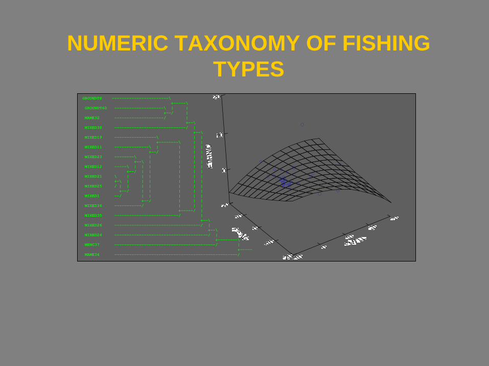
NUMERIC TAXONOMY OF FISHING TYPES
GROUNDT8 -----------------------\ +-----\ GROUNDT40 --------------------\ | | +--/ | MAME32 --------------------/ | +--\ MIXED38 -----------------------------/ | +--\ MIXED19 -----------------\ | | +--------\ | | MIXED11 --------------\ | | | | +--/ | | | MIXED23 --------\ | | | | +--\ | | | | MIXED12 -----\ | | | | | | +--/ | | | | | MIXED21 \ | | | | | | +-\ | | | | | | MIXED25 / | | | | | | | +--/ | | | | | MIXED1 --/ | | | | | +--/ | | | MIXED36 -----------/ | | | +-----/ | MIXED35 --------------------------/ | +--\ MIXED26 -----------------------------------/ | +--\ MIXED24 --------------------------------------/ | +--------\ MENC37 -----------------------------------------/ | +----- MAME34 --------------------------------------------------/

THE PROBLEM
• FROM NORTH CAROLINA NORTH TO THE CANADIAN BORDER THERE ARE ABOUT 5000 BOATS RECORDING LANDINGS IN THE COMMERCIAL FISHERY.
• MANAGEMENT DECISIONS REQUIRE SOCIAL IMPACT ANALYSIS—IDEALLY AVAILABLE PRIOR TO DECISION TIME.
• THERE ARE NOT SUFFICIENT RESOURCES TO ACQUIRE “NECESSARY” INFORMATION ON ALL THESE BOATS.

A POTENTIAL SOLUTION
• IF WE COULD CLASSIFY OR TYPE THESE ESTIMATED 5000 BOATS INTO SMALLER GROUPINGS, SOCIAL IMPACT ANALYSIS DATA FROM A SAMPLE WITHIN WITHIN EACH GROUP WOULD PROVIDE BETTER PREPARATION FOR DECISION MAKING.
• THE PROBLEM, THEREFORE IS ONE OF CLASSIFICATION OR CREATING A TAXONOMY OF FISHING TYPES.

THE METHODS
• FOR THE MOST PART, MODERN BIOLOGY USES SYSTEMATICS TO CLASSIFY ORGANISMS—TOOLS SUCH AS MULTIPLE DISCRIMINANT ANALYSIS AND CLUSTER ANALYSIS.
• IT IS IMPORTANT TO NOTE THAT UNLESS ONE MEASURES EVERY ASPECT OF THE ITEMS TO BE CLASSIFIED, INFORMED, HUMAN DECISION MAKING IS SIGNIFICANTLY INVOLVED IN THE PROCESS.

THE DATABASE ALL STAGES REQUIRE DECISIONS
• Data analyzed are 2009 landings data, by permit, for the North East Region (N=5428).
• Thirty-two types (including a mixed “other”) category were available for analysis. Of the 5428 cases only 3236 manifested landings for the year 2009 and are identified as “active permits.”
• Only the active permits are used in the analysis.

Three basic processes tested for identification of fishing types
• 1) principal component analysis of raw landings data with factor scores calculated for each active permit
• 2) principal component analysis of log landings data with factor scores calculated for each active permit
• 3) hierarchical (average linkage method) cluster analysis of types, using Pearson’s correlation coefficient as the distance metric, with cluster scores for each permit based on log sum of landings within each cluster.

Principal component analysis of raw landings data with factor scores calculated for each active
permit
• With eigen value = 1 for cut-off & varimax rotation 13 components result (66 percent of the variance in the data set).
• The types combined in the fisheries identified by the components make sense (e.g., the first 3 and 5th components made up of mostly deep water fish, but all targeted by trawl nets. The 4th component includes pelagics like mackerel and herring, and so on.

Problem with PC and eigen value cut off of 1
• Some components have only one highly loading type, a phenomena usually avoided by analysts who use PCA as a data reduction technique.
• Solution—use scree-test. • Result: 9 components (54% variance),
which make sense. Fisheries identified make sense, and the types that are not included in a component can be evaluated as separate fisheries.

Principal Component Analysis of Log Data
• many of the types are strongly skewed to the right. A log transformation would improve the reliability of correlations used in PCA and reduce importance of size of landing from the cluster analysis
• To facilitate a cleaner analysis, shrimp, red crab and clams were not used in the PCA & number of components to be rotated was set at 5 (based on scree test). The PCA accounts for 64 percent of the variance, and the structure is relatively clear.

Component scores and K-means cluster analysis of log data
• the results are again unsatisfactory --the largest cluster (cluster 1 with 1578 cases) contains almost one-half the cases & still seems to be based on amount of landings (size).
• the PCA analyses appear to do an excellent job of identifying co-occurring species in landings over the year
• But the calculation of component scores seems to be inappropriate for our purposes

Problem with component scores
• calculated using weights derived from the PCA analysis
• each type contributes to the score for each permit
• This can result in a score that does not clearly define the landings—it has “fuzzy edges.”

Hierarchical Cluster Analysis of Log Data
• cluster analysis of log landing types, using Pearson’s correlation coefficient as the distance metric

Figure 3. Hierarchical cluster analysis of log permit landing data.
Cluster Tree
0.0 0.2 0.4 0.6 0.8 1.0 1.2Distances
LSCALLOPLCLAMS
LREDCRABLOCEANPOUTLMENHADEN
LHERRINGLMACKEREL
LILLEXLREDWHITEHAKE
LDOGFISHLOTHERLBLTILEFISH
LSMESHMULTSLLOLIGOLSCUP
LFLUKELBSB
LWINDOWPANELMONKFISH
LSKATESLWINTERFLOUNDER
LYELLOWTAILFLOUNDERLWITCHFLOUNDER
LPLAICELHADDOCK
LCODLPOLLOCK
LWHITEHAKELREDFISHLHALIBUTLSHRIMP
LLOBSTER

Hierarchical Cluster Analysis of Log Data
• closely parallels the various PCAs • Similar types are combined at various
branchings (distances) in the resulting tree
• co-occurring types can be conceptualized as indicating separate fisheries as with the PCA analyses
• we treat scallops, clams, red crab, ocean pout, shrimp and lobster as separate fisheries

Hierarchical Cluster Analysis of Log Data II
• We group menhaden, herring, mackerel, illex as a fishery.
• Loligo and scup are combined with fluke, then black sea bass. This grouping is then combined with small mesh mullets, then tilefish. This larger grouping is combined with dogfish and “mixed others” and finally red-white hake to form the second multi-type fishery identified by the hierarchical cluster analysis.
• The third multi-type fishery is characterized by closer distances—similar to the PCA analyses

Hierarchical Cluster Analysis of Log Data II
• The tightest cluster includes pollock, white hake and redfish.
• This group is then combined with another tight cluster including witch flounder, haddock, plaice and cod.
• This larger cluster is then combined with the other flounders—winter flounder and yellow tail flounder.
• Monkfish and skates are then combined into the cluster, and finally, at the greatest distance halibut is included in this 3rd cluster.

Cluster scores and clustering boats into the types
• Cluster scores are calculated for each active permit by logging summed landings for each of the 9 fisheries defined by the hierarchical cluster analysis
• Permits (boats) are clustered using K-means cluster analysis of the cluster scores to develop a taxonomy of boats (permit holders) based on similar levels of participation in the fisheries identified by the hierarchical cluster analysis.

CLUSTER(rows) by PPST$(columns) CT DE FL GA MA MD ME NC NE NH NJ NY PA RI VA Tot. 1 3 1 0 0 73 1 339 2 0 11 11 10 0 57 1 509 2 11 0 2 2 160 13 18 12 0 2 92 3 0 5 33 353 3 2 1 1 0 144 13 28 50 0 3 40 76 1 27 30 416 4 0 0 0 0 2 0 58 0 0 0 0 0 0 0 0 60 5 0 1 0 0 164 0 40 0 0 11 3 7 0 14 1 241 6 1 0 0 0 24 2 2 39 0 0 62 17 1 3 35 186 7 10 0 0 0 105 3 10 9 0 13 39 30 0 36 5 260 8 0 0 0 0 5 0 27 0 0 15 0 0 0 0 0 47 9 4 1 0 0 15 1 0 2 0 2 14 24 0 41 0 104 10 8 0 0 0 195 0 572 0 0 31 15 1 0 24 1 847 11 1 0 1 0 48 1 35 0 0 8 23 10 0 7 2 136 12 0 0 0 0 12 0 8 0 1 2 4 0 0 0 0 27 13 0 0 0 0 3 2 2 3 0 0 9 3 0 3 5 30 14 0 0 0 0 0 0 15 0 0 1 0 0 0 0 0 16 15 0 0 0 0 2 0 2 0 0 0 0 0 0 0 0 4 Total 40 4 4 2 952 36 1,156 117 1 99 312 181 2 217 113 3,236


Conclusions
• Overall, this procedure appeared to provide the most useful results—no huge clusters & clusters of permit holders do make sense.
• The future……. • Looking at changes through time • Relating to gear types & income • Other…………………………..