typed open programming - publikationen.sulb.uni-saarland.de · typed open programming a...
TRANSCRIPT
Typed Open Programming
A higher-order, typed approach todynamic modularity and distribution
Preliminary Version
Andreas Rossberg
Dissertation
zur Erlangung des Gradesdes Doktors der Ingenieurwissenschaften
der Naturwissenschaftlich-Technischen Fakultatender Universitat des Saarlandes
Saarbrucken, 5. Januar 2007

Dekan: Prof. Dr. Andreas Schutze
Erstgutachter: Prof. Dr. Gert Smolka
Zweitgutachter: Prof. Dr. Andreas Zeller
ii
Abstract
In this dissertation we develop an approach for reconciling open programming – the developmentof programs that support dynamic exchange of higher-order values with other processes – withstrong static typing in programming languages.
We present the design of a concrete programming language, Alice ML, that consists of aconventional functional language extended with a set of orthogonal features like higher-ordermodules, dynamic type checking, higher-order serialisation, and concurrency. On top of thesea flexible system of dynamic components and a simple but expressive notion of distribution isrealised. The central concept in this design is the package, a first-class value embedding a modulealong with its interface type, which is dynamically checked whenever the module is extracted.
Furthermore, we develop a formal model for abstract types that is not invalidated by thepresence of primitives for dynamic type inspection, as is the case for the standard model basedon existential quantification. For that purpose, we present an idealised language in form ofan extended λ-calculus, which can express dynamic generation of types. This calculus is thefirst to combine and explore the interference of sealing and type inspection with higher-ordersingleton kinds, a feature for expressing sharing constraints on abstract types. A novel notionof abstracton kinds classifies abstract types. Higher-order type and kind coercions allow formodular translucent encapsulation of values at arbitrary type.
Kurzdarstellung
In dieser Dissertation entwickeln wir einen programmiersprachlichen Ansatz zur Verbindungoffener Programmierung – der Entwicklung von Programmen, die das dynamische Laden undAustauschen hoherstufiger Werte mit anderen Prozessen erlauben – mit starker statischer Typ-isierung.
Wir stellen das Design einer konkreten Programmiersprache namens Alice ML vor. Siebesteht aus einer konventionellen funktionalen Sprache, die um einen Satz orthogonaler Konzeptewie hoherstufige Modularisierung, dynamische Typuberprufung, hoherstufige Serialisierung undNebenlaufigkeit erweitert wurde. Darauf aufbauend ist ein flexibles System dynamischer Kom-ponenten sowie ein einfacher aber expressiver Ansatz fur Verteilung verwirklicht. Zentral istdabei das Konzept eines Pakets (package), welches ein Modul in Kombination mit seinemSchnittstellentyp in einen Wert einbettet, und bei der Extraktion des Moduls eine dynamis-che Typuberprufung vornimmt.
Weiterhin entwickeln wir einen theoretischen Ansatz zur Modellierung von abstrakten Typen,welcher im Gegensatz zum herkommlichen formalen Modell existentieller Quantifizierung auchin Gegenwart dynamischer Typinspektion gultig ist. Zu diesem Zweck definieren wir eineidealisierte Sprache in Form eines erweiterten λ-Kalkuls, der dynamische Typgenerierungausdrucken kann. Der Kalkul kombiniert diese erstmals mit hoherstufigen ”Singleton Kinds,einem Sprachkonstrukt, welches Gleichheit von Typen ausdrucken kann. Zur Klassifizierungabstrakter Typen werden Abstraktions-Kinds als verwandtes Konzept entwickelt. HoherstufigeKonversionen auf Term- und Typebene erlauben zudem die nachtragliche modulare Enkap-sulierung von Werten beliebigen Typs.
iii
Zusammenfassung
Die zunehmende Verbreitung des Internets hat begonnen, die Struktur von Software nachhaltigzu verandern. An die Stelle von in sich geschlossenen Programmen, die nur lokal operieren,treten mehr und mehr offene Applikationen, die dynamisch Daten mit anderen Prozessen imNetzwerk austauschen, oder von dort sogar neue Funktionalitat beziehen. Das offensichtlichsteBeispiel fur ein Programm dieser Kategorie ist ein Web-Browser.
Auf programmiersprachlicher Ebene erfordert dieser Paradigmenwechsel eine verbesserte Un-terstutzung offener Programmierung, zu der wir Konzepte wie Modularitat, Dynamik, Porta-bilitat, Sicherheit, Verteilung und Nebenlaufigkeit zahlen. Nur wenige existierende Sprachensind bisher darauf ausgelegt. Zu ihnen gehoren vor allem die zu diesem Zweck entwickelteobjektorientierte Sprache Java, die mittlerweile weite industrielle Verbreitung gefunden hat,und die im akademischen Umfeld entwickelte nebenlaufige Constraint-Sprache Oz. Diese setztentsprechende Konzepte noch weitaus konsequenter um, insbesondere durch die einheitlicheReprasentation von Programmkomponenten und externen Daten, so dass beide beliebig gemis-cht werden konnen.
Diese Dissertation widmet sich einem spezifischen Aspekt offener Programmierung, der bis-lang von keinem der Vertreter auf befriedigende Weise gelost wurde: der Kombination offenerProgrammierung mit einem expressiven, starken Typsystem. Ein Typsystem ist ein in die Pro-grammiersprache integriertes formales Werkzeug zur automatischen Verifikation bestimmter Pro-grammeigenschaften. Es weist jedem Programmkonstrukt einen Typ zu, eine logische Formel,die das bei Ausfuhrung des Konstrukts zu erwartende Resultat klassifiziert. Die damit moglichenKonsistenzprufungen konnen die Zuverlassigkeit von Software verbessern. Moderne Program-miersprachen bieten zudem die Moglichkeit, die Typstruktur um benutzerdefinierte, sogenannteabstrakte Typen zu erweitern, welche die Festlegung gewisser Zugriffsbeschrankungen erlauben.Wenn die Semantik der Programmiersprache verhindert, dass diese Zugriffsbeschrankungen um-gangen werden konnen, so spricht man von Abstraktionssicherheit. Diese garantiert Modu-laritatseigenschaften und steigert damit vor allem die Wartbarkeit von Programmen.
Typuberprufungen erfolgen naturgemass vor der Ausfuhrung eines Programmes, ublicherweisedurch den Ubersetzer der verwendeten Programmiersprache. Dadurch entsteht ein inharenterKonflikt mit offener Programmierung, da in einem offenen Ansatz im Allgemeinen nicht alleProgrammteile vorweg bekannt sind und analysiert werden konnen. Es ist deshalb unausweich-lich, bestimmte Typuberprufungen in die Laufzeit des Programms zu verlagern. Ein seit langembekannter Ansatz dafur ist die Einbringung eines speziellen universellen Typs Dynamic, derWerte der Sprache gepaart mit ihrem jeweiligen Typ beinhaltet. Die Extraktion eines Wertes er-folgt explizit und erfordert die Angabe eines oder mehrerer erwarteter Zieltypen, die dynamischabgeglichen werden. Leider haben sich Dynamics jedoch in der Praxis als zu unhandlich er-wiesen. Zudem ergeben sich durch die Moglichkeit des dynamischen Typabgleichs semantischeImplikationen, die unter anderem die Abstraktionssicherheit abstrakter Typen beeintrachtigen.
Wir nahern uns diesen Problemen von zwei Seiten an. Zum einen beschreiben wir das Designeiner konkreten Sprache names Alice ML, welche typisierte offene Programmierung ermoglicht.Dabei handelt es sich um einen Dialekt der funktionalen Sprache Standard ML, die durch einenrelativ kleinen Satz orthogonaler und hinreichen einfacher Sprachkonstrukte erweitert wurde.Dabei handelt es sich zunachst um Pickling zum serialisierten Import und Export hoherstufiger
iv
Werte, verschiedene Formen von Futures fur die Synchronisation nebenlaufiger Berechnungen,sowie Module hoherer Ordnung, welche die Sprache um wichtige Abstraktionsmoglichkeitenerganzen. Die meisten dieser Konstrukte sind bekannt und fur sich gut verstanden, aber bishernicht in dieser Form und zu diesem Zweck in einem koharenten Design integriert worden. Neuist ausserdem das zentrale Konzept von Paketen (packages), welches das Kernproblem der dy-namischen Typisierung lost. Es ahnelt der Idee von Dynamics, jedoch werden nicht einzelneWerte, sondern komplette Module eingebettet. Die feinkornige Typunterscheidung weicht soeinem strukturellen Inklusionstest auf Modulschnittstellen, der robust gegenuber Erweiterun-gen ist und eine Handhabung auf hohem Abstraktionsgrad erlaubt. Auf Grundlage dieser Ba-siskonzepte definiert die Sprache einen flexiblen, typsicheren Begriff von Komponenten, der nichtnur bedarfsgetriebenes dynamisches Laden ermoglicht, sondern Komponenten als Werte ersterKlasse verfugbar macht, die dynamisch berechnet und aus einem Prozess exportiert werdenkonnen. Mit Hilfe dieser Idee wiederum ist ein vergleichsweise einfacher aber expressiver Ansatzfur verteilte Programmierung moglich, bei dem Verbindungen zwischen Prozessen durch deninitialen Austausch einer dynamisch berechneten Komponente aufgebaut werden. Das Konzeptvon programmierbaren Komponentenmanagern erlaubt es dem Empfangerprozess dabei, gezielteSicherheitsstrategien durch Einschrankung der Importrechte fur die empfangene Komponente zurealisieren. Eine nahezu vollstandige Implementation von Alice ML wurde realisiert und stehtals offene Software zur Verfugung.
Zum anderen entwickeln wir einen theoretischen Ansatz zur Modellierung von Typabstrak-tion, der Abstraktionssicherheit auch in Gegenwart dynamischer Typinspektion sicherstellt. Zudiesem Zweck fuhren wir eine idealisierte Formalisierung der Sprache Alice ML ein, die aufdem polymorphen λ-Kalkul basiert. Sie modelliert zentrale Konzepte des Typ- und Modulsys-tems: hoherstufige Typen spiegeln Polymorphismus und parametrisierte Module wider, SingletonKinds konnen Gleichheit von abstrakten Typen ausdrucken (type sharing), ein Konditional uberTypen erlaubt Typinspektion und das Kodieren von Paketen, Subtyping und Subkinding erfassenSchnittstelleninklusion. Zudem wird Pickling als spezielles Konstrukt eingefuhrt, welches dasHantieren mit potentiell nicht-wohlgeformten Werten ermoglicht. Das wichtigste Merkmal istjedoch dynamische Typgenerierung, welche abstrakte Typen realisiert. Der Kalkul modelliertdamit erstmals die Interaktion von hoherstufiger dynamischer Typabstraktion mit dynamis-chem Typ-Sharing, welche zentral ist fur die Typisierung von Alice ML. Typgenerierung gehteinher mit der neu entwickelten Idee von Abstraktions-Kinds, welche zur feinkornigen Klassi-fikation abstrakter Typen hoherer Ordnung benutzt werden. Auf Termebene erlauben explizite,hoherstufige Konversionen (coercions) die nachtragliche Enkapsulation beliebig komplexer Ob-jekte in punktuell abstrahierte Typen. Wir beweisen die Entscheidbarkeit des Typsystems, seineKorrektheit in Bezug auf die operationale Semantik des Kalkuls, sowie eine einfache Eigenschaftvon Abstraktionssicherheit.
v

vi
Contents
1. Introduction 1
1.1. Type Systems . . . . . . . . . . . . . . . . . . . . . . . . . . . . . . . . . . . . . 2
1.1.1. Type Abstraction . . . . . . . . . . . . . . . . . . . . . . . . . . . . . . . 3
1.2. Open Programming . . . . . . . . . . . . . . . . . . . . . . . . . . . . . . . . . . 4
1.2.1. Java . . . . . . . . . . . . . . . . . . . . . . . . . . . . . . . . . . . . . . 5
1.2.2. Oz . . . . . . . . . . . . . . . . . . . . . . . . . . . . . . . . . . . . . . . 6
1.3. Typed Open Programming . . . . . . . . . . . . . . . . . . . . . . . . . . . . . . 6
1.3.1. Java . . . . . . . . . . . . . . . . . . . . . . . . . . . . . . . . . . . . . . 7
1.3.2. Dynamics . . . . . . . . . . . . . . . . . . . . . . . . . . . . . . . . . . . 8
1.4. Contribution . . . . . . . . . . . . . . . . . . . . . . . . . . . . . . . . . . . . . . 9
1.5. Structure . . . . . . . . . . . . . . . . . . . . . . . . . . . . . . . . . . . . . . . . 11
I. Introducing Alice ML 13
2. Overview 15
2.1. Standard ML Heritage . . . . . . . . . . . . . . . . . . . . . . . . . . . . . . . . 15
2.2. Extensions and Oz Heritage . . . . . . . . . . . . . . . . . . . . . . . . . . . . . 16
2.3. The Alice Programming System . . . . . . . . . . . . . . . . . . . . . . . . . . . 17
2.4. Summary . . . . . . . . . . . . . . . . . . . . . . . . . . . . . . . . . . . . . . . . 17
3. Higher-Order Modules 19
3.1. Higher-Order Functors . . . . . . . . . . . . . . . . . . . . . . . . . . . . . . . . 20
3.2. Local Modules . . . . . . . . . . . . . . . . . . . . . . . . . . . . . . . . . . . . . 23
3.3. Local and Abstract Signatures . . . . . . . . . . . . . . . . . . . . . . . . . . . . 24
3.3.1. Local Signatures . . . . . . . . . . . . . . . . . . . . . . . . . . . . . . . 24
3.3.2. Abstract Signatures . . . . . . . . . . . . . . . . . . . . . . . . . . . . . . 25
3.4. Related Work . . . . . . . . . . . . . . . . . . . . . . . . . . . . . . . . . . . . . 26
3.5. Summary . . . . . . . . . . . . . . . . . . . . . . . . . . . . . . . . . . . . . . . . 27
4. Packages 29
4.1. Basics . . . . . . . . . . . . . . . . . . . . . . . . . . . . . . . . . . . . . . . . . . 30
4.2. Persistence . . . . . . . . . . . . . . . . . . . . . . . . . . . . . . . . . . . . . . . 31
4.3. Dynamic Type Matching . . . . . . . . . . . . . . . . . . . . . . . . . . . . . . . 32
4.4. Dynamic Type Sharing . . . . . . . . . . . . . . . . . . . . . . . . . . . . . . . . 33
4.4.1. Package Signature Refinement . . . . . . . . . . . . . . . . . . . . . . . . 34
4.5. Parametricity . . . . . . . . . . . . . . . . . . . . . . . . . . . . . . . . . . . . . 35
4.5.1. Working Around Parametricity . . . . . . . . . . . . . . . . . . . . . . . 36
4.6. Abstract Types . . . . . . . . . . . . . . . . . . . . . . . . . . . . . . . . . . . . 37
4.6.1. Internal and External View of Abstraction . . . . . . . . . . . . . . . . . 38
4.7. Typeful Dynamic Programming . . . . . . . . . . . . . . . . . . . . . . . . . . . 39
4.8. Related Work . . . . . . . . . . . . . . . . . . . . . . . . . . . . . . . . . . . . . 41
vii
Contents
4.9. Summary . . . . . . . . . . . . . . . . . . . . . . . . . . . . . . . . . . . . . . . . 41
5. Pickling 43
5.1. Pickles . . . . . . . . . . . . . . . . . . . . . . . . . . . . . . . . . . . . . . . . . 43
5.2. Type checking and verification . . . . . . . . . . . . . . . . . . . . . . . . . . . . 44
5.3. Resources and Security . . . . . . . . . . . . . . . . . . . . . . . . . . . . . . . . 47
5.3.1. State . . . . . . . . . . . . . . . . . . . . . . . . . . . . . . . . . . . . . . 47
5.4. Abstraction Safety . . . . . . . . . . . . . . . . . . . . . . . . . . . . . . . . . . . 48
5.5. Transformations . . . . . . . . . . . . . . . . . . . . . . . . . . . . . . . . . . . . 49
5.6. Modules . . . . . . . . . . . . . . . . . . . . . . . . . . . . . . . . . . . . . . . . 50
5.7. Related Work . . . . . . . . . . . . . . . . . . . . . . . . . . . . . . . . . . . . . 51
5.8. Summary . . . . . . . . . . . . . . . . . . . . . . . . . . . . . . . . . . . . . . . . 52
6. Futures 53
6.1. Concurrency . . . . . . . . . . . . . . . . . . . . . . . . . . . . . . . . . . . . . . 54
6.1.1. Synchronisation . . . . . . . . . . . . . . . . . . . . . . . . . . . . . . . . 54
6.1.2. Asynchronicity . . . . . . . . . . . . . . . . . . . . . . . . . . . . . . . . 55
6.2. Laziness . . . . . . . . . . . . . . . . . . . . . . . . . . . . . . . . . . . . . . . . 56
6.3. Failure . . . . . . . . . . . . . . . . . . . . . . . . . . . . . . . . . . . . . . . . . 57
6.4. Promises . . . . . . . . . . . . . . . . . . . . . . . . . . . . . . . . . . . . . . . . 58
6.5. Locking . . . . . . . . . . . . . . . . . . . . . . . . . . . . . . . . . . . . . . . . . 60
6.5.1. Promises Revisited . . . . . . . . . . . . . . . . . . . . . . . . . . . . . . 60
6.6. Modules . . . . . . . . . . . . . . . . . . . . . . . . . . . . . . . . . . . . . . . . 61
6.7. Types . . . . . . . . . . . . . . . . . . . . . . . . . . . . . . . . . . . . . . . . . . 62
6.8. Related Work . . . . . . . . . . . . . . . . . . . . . . . . . . . . . . . . . . . . . 63
6.9. Summary . . . . . . . . . . . . . . . . . . . . . . . . . . . . . . . . . . . . . . . . 64
7. Components 65
7.1. Compilation Units . . . . . . . . . . . . . . . . . . . . . . . . . . . . . . . . . . . 66
7.1.1. Implicit import signatures . . . . . . . . . . . . . . . . . . . . . . . . . . 67
7.1.2. Example: A simple stand-alone application . . . . . . . . . . . . . . . . 67
7.2. Computed Components . . . . . . . . . . . . . . . . . . . . . . . . . . . . . . . . 67
7.2.1. Pickling Components . . . . . . . . . . . . . . . . . . . . . . . . . . . . . 71
7.3. Dynamic Linking . . . . . . . . . . . . . . . . . . . . . . . . . . . . . . . . . . . 72
7.4. Component Managers . . . . . . . . . . . . . . . . . . . . . . . . . . . . . . . . . 73
7.5. Resources and Sandboxing . . . . . . . . . . . . . . . . . . . . . . . . . . . . . . 74
7.6. Decomposition of the Component System . . . . . . . . . . . . . . . . . . . . . . 75
7.6.1. Components . . . . . . . . . . . . . . . . . . . . . . . . . . . . . . . . . . 75
7.6.2. Examples . . . . . . . . . . . . . . . . . . . . . . . . . . . . . . . . . . . 76
7.6.3. Component Managers . . . . . . . . . . . . . . . . . . . . . . . . . . . . 77
7.6.4. Program Execution . . . . . . . . . . . . . . . . . . . . . . . . . . . . . . 79
7.7. Type Propagation . . . . . . . . . . . . . . . . . . . . . . . . . . . . . . . . . . . 80
7.8. Static Linking . . . . . . . . . . . . . . . . . . . . . . . . . . . . . . . . . . . . . 81
7.9. Related Work . . . . . . . . . . . . . . . . . . . . . . . . . . . . . . . . . . . . . 82
7.10. Summary . . . . . . . . . . . . . . . . . . . . . . . . . . . . . . . . . . . . . . . . 86
viii
Contents
8. Distribution 87
8.1. Proxies . . . . . . . . . . . . . . . . . . . . . . . . . . . . . . . . . . . . . . . . . 888.1.1. Example: Remote References . . . . . . . . . . . . . . . . . . . . . . . . 91
8.1.2. Proxy Failure . . . . . . . . . . . . . . . . . . . . . . . . . . . . . . . . . 928.2. Tickets . . . . . . . . . . . . . . . . . . . . . . . . . . . . . . . . . . . . . . . . . 92
8.2.1. Bi- and multi-directional Connections . . . . . . . . . . . . . . . . . . . 938.2.2. Example: Chat Room . . . . . . . . . . . . . . . . . . . . . . . . . . . . 94
8.3. Remote Execution . . . . . . . . . . . . . . . . . . . . . . . . . . . . . . . . . . . 958.3.1. Example: Distributed Search . . . . . . . . . . . . . . . . . . . . . . . . 95
8.4. Safety . . . . . . . . . . . . . . . . . . . . . . . . . . . . . . . . . . . . . . . . . . 97
8.4.1. Type Safety and Verification . . . . . . . . . . . . . . . . . . . . . . . . . 978.4.2. Resources . . . . . . . . . . . . . . . . . . . . . . . . . . . . . . . . . . . 988.4.3. Other Security Concerns . . . . . . . . . . . . . . . . . . . . . . . . . . . 99
8.5. Related Work . . . . . . . . . . . . . . . . . . . . . . . . . . . . . . . . . . . . . 998.6. Summary . . . . . . . . . . . . . . . . . . . . . . . . . . . . . . . . . . . . . . . . 101
9. Implementation and Outlook 103
9.1. Architecture of the Alice System . . . . . . . . . . . . . . . . . . . . . . . . . . . 1039.2. Other Language Extensions in Alice ML . . . . . . . . . . . . . . . . . . . . . . 1039.3. Limitations . . . . . . . . . . . . . . . . . . . . . . . . . . . . . . . . . . . . . . . 1049.4. Future Work . . . . . . . . . . . . . . . . . . . . . . . . . . . . . . . . . . . . . . 105
9.4.1. Possible Extensions . . . . . . . . . . . . . . . . . . . . . . . . . . . . . . 1059.4.2. Language Specification . . . . . . . . . . . . . . . . . . . . . . . . . . . . 1059.4.3. Implementation . . . . . . . . . . . . . . . . . . . . . . . . . . . . . . . . 107
II. Theory 109
10.A Calculus for Components 111
10.1. Core Language: Higher-order Polymorphic λ-calculus . . . . . . . . . . . . . . . 11210.2. Modules: Existential Types and Higher-order Quantification . . . . . . . . . . . 11410.3. Type Sharing and Translucency: Singleton Kinds and Subtyping . . . . . . . . . 11710.4. Dynamic Typing: Type Analysis . . . . . . . . . . . . . . . . . . . . . . . . . . . 118
10.5. Loss of Parametricity and Abstraction Safety . . . . . . . . . . . . . . . . . . . . 12010.6. Abstraction Safety: Dynamic Generativity . . . . . . . . . . . . . . . . . . . . . 12310.7. Sealing: Higher-order Coercions and Generativity . . . . . . . . . . . . . . . . . 12410.8. Pickling . . . . . . . . . . . . . . . . . . . . . . . . . . . . . . . . . . . . . . . . . 12610.9. Summary . . . . . . . . . . . . . . . . . . . . . . . . . . . . . . . . . . . . . . . . 127
11.The Type Language 129
11.1. Basic System . . . . . . . . . . . . . . . . . . . . . . . . . . . . . . . . . . . . . . 12911.1.1. Environments . . . . . . . . . . . . . . . . . . . . . . . . . . . . . . . . . 13011.1.2. Kinds . . . . . . . . . . . . . . . . . . . . . . . . . . . . . . . . . . . . . 13011.1.3. Types . . . . . . . . . . . . . . . . . . . . . . . . . . . . . . . . . . . . . 13211.1.4. Terms . . . . . . . . . . . . . . . . . . . . . . . . . . . . . . . . . . . . . 136
11.2. Singletons . . . . . . . . . . . . . . . . . . . . . . . . . . . . . . . . . . . . . . . 136
11.2.1. Ground Singletons . . . . . . . . . . . . . . . . . . . . . . . . . . . . . . 13611.2.2. Higher-Order Singletons . . . . . . . . . . . . . . . . . . . . . . . . . . . 13811.2.3. βη-Equivalences . . . . . . . . . . . . . . . . . . . . . . . . . . . . . . . . 139
11.3. Abstraction Kinds . . . . . . . . . . . . . . . . . . . . . . . . . . . . . . . . . . . 140
ix
Contents
11.3.1. Singletons over Abstraction Kinds . . . . . . . . . . . . . . . . . . . . . 140
11.4. Algorithmic Formulations . . . . . . . . . . . . . . . . . . . . . . . . . . . . . . . 141
11.4.1. Type and Kind Equivalence . . . . . . . . . . . . . . . . . . . . . . . . . 141
11.4.2. Subkinding . . . . . . . . . . . . . . . . . . . . . . . . . . . . . . . . . . 144
11.4.3. Kind Synthesis . . . . . . . . . . . . . . . . . . . . . . . . . . . . . . . . 145
11.4.4. Subtyping . . . . . . . . . . . . . . . . . . . . . . . . . . . . . . . . . . . 146
11.5. Related Work . . . . . . . . . . . . . . . . . . . . . . . . . . . . . . . . . . . . . 148
11.5.1. Typed Lambda Calculi . . . . . . . . . . . . . . . . . . . . . . . . . . . . 148
11.5.2. Singletons . . . . . . . . . . . . . . . . . . . . . . . . . . . . . . . . . . . 148
11.5.3. Type Names, Environment and Abstraction Kinds . . . . . . . . . . . . 149
11.6. Summary . . . . . . . . . . . . . . . . . . . . . . . . . . . . . . . . . . . . . . . . 149
12.The Term Language 151
12.1. Typing . . . . . . . . . . . . . . . . . . . . . . . . . . . . . . . . . . . . . . . . . 151
12.1.1. Principality . . . . . . . . . . . . . . . . . . . . . . . . . . . . . . . . . . 151
12.2. Reduction . . . . . . . . . . . . . . . . . . . . . . . . . . . . . . . . . . . . . . . 153
12.3. Type Analysis . . . . . . . . . . . . . . . . . . . . . . . . . . . . . . . . . . . . . 154
12.3.1. Semantics . . . . . . . . . . . . . . . . . . . . . . . . . . . . . . . . . . . 154
12.3.2. Packages . . . . . . . . . . . . . . . . . . . . . . . . . . . . . . . . . . . . 155
12.3.3. Recursion . . . . . . . . . . . . . . . . . . . . . . . . . . . . . . . . . . . 156
12.4. Type Generation . . . . . . . . . . . . . . . . . . . . . . . . . . . . . . . . . . . . 156
12.4.1. Type Heap . . . . . . . . . . . . . . . . . . . . . . . . . . . . . . . . . . . 156
12.4.2. Analysing Generated Types . . . . . . . . . . . . . . . . . . . . . . . . . 157
12.5. Coercions . . . . . . . . . . . . . . . . . . . . . . . . . . . . . . . . . . . . . . . . 158
12.6. Pickling . . . . . . . . . . . . . . . . . . . . . . . . . . . . . . . . . . . . . . . . . 158
12.7. Algorithmic Type Checking . . . . . . . . . . . . . . . . . . . . . . . . . . . . . . 159
12.8. Soundness . . . . . . . . . . . . . . . . . . . . . . . . . . . . . . . . . . . . . . . 160
12.9. Opacity . . . . . . . . . . . . . . . . . . . . . . . . . . . . . . . . . . . . . . . . . 161
12.10.Related Work . . . . . . . . . . . . . . . . . . . . . . . . . . . . . . . . . . . . . 162
12.10.1.Type Analysis and Dynamics . . . . . . . . . . . . . . . . . . . . . . . . 162
12.10.2.Term Name Generation . . . . . . . . . . . . . . . . . . . . . . . . . . . 163
12.10.3.Abstraction Safety and Type Generation . . . . . . . . . . . . . . . . . . 164
12.10.4.Opacity and Proof Techniques . . . . . . . . . . . . . . . . . . . . . . . . 165
12.11. Summary . . . . . . . . . . . . . . . . . . . . . . . . . . . . . . . . . . . . . . . . 166
13.Higher-Order Abstraction 167
13.1. Higher-Order Generativity . . . . . . . . . . . . . . . . . . . . . . . . . . . . . . 167
13.1.1. Type Generation . . . . . . . . . . . . . . . . . . . . . . . . . . . . . . . 168
13.1.2. Abstraction Kinds . . . . . . . . . . . . . . . . . . . . . . . . . . . . . . 168
13.1.3. Type Coercions . . . . . . . . . . . . . . . . . . . . . . . . . . . . . . . . 170
13.2. Higher-Order Type Coercions . . . . . . . . . . . . . . . . . . . . . . . . . . . . 171
13.2.1. Semantics . . . . . . . . . . . . . . . . . . . . . . . . . . . . . . . . . . . 172
13.2.2. Monomorphic Coercions . . . . . . . . . . . . . . . . . . . . . . . . . . . 173
13.2.3. Polymorphic Coercions . . . . . . . . . . . . . . . . . . . . . . . . . . . . 174
13.2.4. Abstract Coercions . . . . . . . . . . . . . . . . . . . . . . . . . . . . . . 175
13.3. Kind Coercions . . . . . . . . . . . . . . . . . . . . . . . . . . . . . . . . . . . . 176
13.3.1. Definition and Semantics . . . . . . . . . . . . . . . . . . . . . . . . . . . 177
13.3.2. Abstraction Kinds Revisited . . . . . . . . . . . . . . . . . . . . . . . . . 179
13.3.3. Type Coercions Revisited . . . . . . . . . . . . . . . . . . . . . . . . . . 179
x
Contents
13.3.4. The Concrete Kind Restriction . . . . . . . . . . . . . . . . . . . . . . . 180
13.4. Properties . . . . . . . . . . . . . . . . . . . . . . . . . . . . . . . . . . . . . . . 181
13.4.1. Algorithmic Type Synthesis . . . . . . . . . . . . . . . . . . . . . . . . . 18113.4.2. Soundness . . . . . . . . . . . . . . . . . . . . . . . . . . . . . . . . . . . 182
13.4.3. Opacity . . . . . . . . . . . . . . . . . . . . . . . . . . . . . . . . . . . . 183
13.5. Sealing . . . . . . . . . . . . . . . . . . . . . . . . . . . . . . . . . . . . . . . . . 18313.6. Discussion and Related Work . . . . . . . . . . . . . . . . . . . . . . . . . . . . . 185
13.6.1. Design Space . . . . . . . . . . . . . . . . . . . . . . . . . . . . . . . . . 185
13.6.2. Related Work . . . . . . . . . . . . . . . . . . . . . . . . . . . . . . . . . 18613.7. Summary . . . . . . . . . . . . . . . . . . . . . . . . . . . . . . . . . . . . . . . . 188
14.Conclusion and Future Work 189
14.1. Conclusion . . . . . . . . . . . . . . . . . . . . . . . . . . . . . . . . . . . . . . . 189
14.2. Future Work . . . . . . . . . . . . . . . . . . . . . . . . . . . . . . . . . . . . . . 189
A. Calculus Summary 193
A.1. Basic System . . . . . . . . . . . . . . . . . . . . . . . . . . . . . . . . . . . . . . 193A.1.1. Syntax . . . . . . . . . . . . . . . . . . . . . . . . . . . . . . . . . . . . . 193
A.1.2. Derived Forms . . . . . . . . . . . . . . . . . . . . . . . . . . . . . . . . 193
A.1.3. Static Semantics . . . . . . . . . . . . . . . . . . . . . . . . . . . . . . . 194
A.1.4. Derived Rules . . . . . . . . . . . . . . . . . . . . . . . . . . . . . . . . . 198A.1.5. Dynamic Semantics . . . . . . . . . . . . . . . . . . . . . . . . . . . . . . 199
A.2. Higher-Order Extensions . . . . . . . . . . . . . . . . . . . . . . . . . . . . . . . 199
A.2.1. Syntax . . . . . . . . . . . . . . . . . . . . . . . . . . . . . . . . . . . . . 199A.2.2. Derived Forms . . . . . . . . . . . . . . . . . . . . . . . . . . . . . . . . 200
A.2.3. Static Semantics . . . . . . . . . . . . . . . . . . . . . . . . . . . . . . . 200
A.2.4. Derived Rules . . . . . . . . . . . . . . . . . . . . . . . . . . . . . . . . . 201A.2.5. Dynamic Semantics . . . . . . . . . . . . . . . . . . . . . . . . . . . . . . 202
B. Encoding Modules 203
C. Proofs of Type Level Properties 207
C.1. Declarative Properties . . . . . . . . . . . . . . . . . . . . . . . . . . . . . . . . . 207
C.1.1. Preliminaries . . . . . . . . . . . . . . . . . . . . . . . . . . . . . . . . . 207
C.1.2. Validity and Functionality . . . . . . . . . . . . . . . . . . . . . . . . . . 210C.2. Derivable Rules . . . . . . . . . . . . . . . . . . . . . . . . . . . . . . . . . . . . 218
C.2.1. Higher-Order Singletons . . . . . . . . . . . . . . . . . . . . . . . . . . . 218
C.2.2. βη-Equivalence . . . . . . . . . . . . . . . . . . . . . . . . . . . . . . . . 222
C.3. Algorithmic Formulations . . . . . . . . . . . . . . . . . . . . . . . . . . . . . . . 223C.3.1. Type Equivalence . . . . . . . . . . . . . . . . . . . . . . . . . . . . . . . 223
C.3.2. Subkinding . . . . . . . . . . . . . . . . . . . . . . . . . . . . . . . . . . 229
C.3.3. Kind Synthesis . . . . . . . . . . . . . . . . . . . . . . . . . . . . . . . . 230C.3.4. Subtyping . . . . . . . . . . . . . . . . . . . . . . . . . . . . . . . . . . . 235
D. Proofs of Term Level Properties 243
D.1. Declarative Properties . . . . . . . . . . . . . . . . . . . . . . . . . . . . . . . . . 243
D.2. Algorithmic Type Checking . . . . . . . . . . . . . . . . . . . . . . . . . . . . . . 245
D.3. Soundness . . . . . . . . . . . . . . . . . . . . . . . . . . . . . . . . . . . . . . . 247D.3.1. Preservation . . . . . . . . . . . . . . . . . . . . . . . . . . . . . . . . . . 247
D.3.2. Progress . . . . . . . . . . . . . . . . . . . . . . . . . . . . . . . . . . . . 250
xi
Contents
D.4. Opacity . . . . . . . . . . . . . . . . . . . . . . . . . . . . . . . . . . . . . . . . . 252
E. Proofs for Higher-Order Abstraction 255
E.1. Kind Coercions . . . . . . . . . . . . . . . . . . . . . . . . . . . . . . . . . . . . 255E.2. Abstraction Kinds . . . . . . . . . . . . . . . . . . . . . . . . . . . . . . . . . . . 264E.3. Higher-Order Generativity and Type Coercions . . . . . . . . . . . . . . . . . . 267
E.3.1. Declarative Properties . . . . . . . . . . . . . . . . . . . . . . . . . . . . 267E.3.2. Algorithmic Type Synthesis . . . . . . . . . . . . . . . . . . . . . . . . . 268E.3.3. Preservation . . . . . . . . . . . . . . . . . . . . . . . . . . . . . . . . . . 270E.3.4. Progress . . . . . . . . . . . . . . . . . . . . . . . . . . . . . . . . . . . . 275E.3.5. Opacity . . . . . . . . . . . . . . . . . . . . . . . . . . . . . . . . . . . . 277
E.4. Sealing . . . . . . . . . . . . . . . . . . . . . . . . . . . . . . . . . . . . . . . . . 277
F. Index of Propositions 279
xii
1. Introduction
Computing used to be a simple affair. A user sat down in front of a dedicated machine and fedit a program whose task was to solve a well-defined problem. The computer executed the stepsdictated by the program, one after the other. It was not long, and programs became interactive,had to react to the user’s input while running. But still, the user worked with a single machine,and usually a single program at a time, and interaction largely followed linear paths.
And then came the Internet. . .
There no longer is such a thing as “a program”, running on “a computer”. Computers forma world-wide network of communicating processes. Activities like surfing the Web consist ofconcurrent interaction with countless processes, running simultaneously, on a large number ofdistant and diverse machines. These processes have to exchange all kinds of functionality anddata to please anonymous users and handle their increasingly demanding requests. Sometimesthey may fail to do so, for a variety of challenging reasons. And a few of these processes eventurn out to be evil, trying to disturb the work of others on purpose!
The world of computing sure has become complicated.
Of course, we are vastly simplifying matters here, for sheer effect. But the point is: program-ming in today’s world tends to be fundamentally different from what it used to be. Complexissues like concurrency, distribution, failure, and security could largely be ignored in traditionalprogramming. They no longer can be today – programs now have to be open to communicate,be extended, move around, adapt.
The primary tool for constructing programs is – and probably will be for a long time to come– a programming language. So how have programming languages, and underlying concepts, beenadapted to these fundamental changes? The sad truth is, most of them have not. Or have onlyin patched-up ways, which hardly appear adequate under scrutiny. And those languages thatdo offer serious support for open programming usually pay with substantial compromises inlanguage design and semantics.
In this dissertation, we are trying to address some of the issues raised by an open approach toprogramming. We present a language design that features a novel combination of programminglanguage concepts to support open programming in a coherent manner. We especially focus onone central but critical feature of programming languages: their type system. A type systemhelps to improve correctness and safety by performing automated consistency checks when aprogram is translated. Our main objective is to explore ways to encompass the incompletetype information available during translation of open programs, and ideally, to extend the typesystem’s utility to the run-time of a program. Our thesis is as simple as the following:
Type systems can be reconciled with open programming without sacrificing their de-sirable properties.
The remainder of this chapter is dedicated to explaining, in a little more depth, the purpose oftype systems and what their desirable properties are, our understanding of open programming,and the difficulties in combining both. In due course, we will have a brief look at the currentstate of the art in the programming language mainstream. Finally, we present our take onattempting to improving this state.
1
1. Introduction
1.1. Type Systems
Most modern, high-level programming languages incorporate a type system. By that, we under-stand a formal discipline according to Pierce’s definition [Pie02]:
A type system is a tractable syntactic method for proving the absence of certain pro-gram behaviours by classifying phrases according to the kinds of values they compute.
This definition implies that a type system is inherently static. Nevertheless, we will sometimesexplicitly talk about static typing, to differentiate clearly from dynamically checked languageslike Lisp or Oz that are often characterised as “dynamically typed”, by slight abuse of terminology.In accordance with standard literature [Car97b] we will classify the latter languages as untyped(but safe).
The essence of static typing is to classify the objects used and computed in a program withdescriptive entities called types. Typing thus provides a method for statically stating and as-serting certain invariants about program objects. It can also be used to express domain-specificconcepts and invariants on a more abstract level. If understood as a tool, the advantages ofstatic typing are hence many-fold:
• Specification. A program design largely consists of the specification of data structuresand operations. Types provide a precise language to express and communicate essentialinformation about such designs on varying levels of abstraction.
• Verified Documentation. Non-trivial programs are not understandable without a cer-tain amount of inline documentation. Type annotations allow expressing a vital part ofthis documentation within the programming language itself. That documentation cannever get “out of sync”, because it is checked by the compiler.
• Error Detection. A type system identifies and locates a large class of problems beforea program is run. The strong invariants thus provided also increase the locality of othererrors, reducing the search space for finding them. That becomes the more important themore complex data structures and operators grow.
• Encapsulation. Large programs have to be decomposed into smaller entities of restrictedresponsibility, usually called modules. In order to keep module interference manageable, allinteraction between modules should be explicitly restricted, so that individual modules canestablish internal invariants. Abstract types can enforce modular separation and interfacecompliance.
• Maintenance. Modifying existing programs is a difficult task, because local changesmight require unanticipated adaption of remote program parts. A type checker often canpoint out inconsistencies after program changes and extensions.
• Safety. A sound type system ensures that a program accesses the machine’s resourcesin valid ways only. For instance, memory safety is a property which precludes access tomemory in uncontrolled ways that may lead to – potentially fatal – internal inconsistenciesor interference with other programs.
• Security. A rich enough type system can even ensure absence of certain security vi-olations, like attempting access to delicate resources or restricted parts of the system.Innovative type theories for purposes like this are an active research topic.
2
1.1. Type Systems
• Efficiency. A type-correct program is guaranteed not to encounter certain conditionsduring execution. Some aspects of a runtime system can be simplified and made moreefficient by being able to ignore these conditions. Moreover, a compiler can make use ofthe typing invariants derived for individual programs to generate specialised code.
It should be mentioned that a type system also is a useful tool for the language designer andresearcher: it provides a well-founded organisation principle for designing new language features,as well as a formal framework for proving certain properties about language constructs.
Of course, nothing comes without a price, so there are well-known disadvantages to statictyping, which have caused even some recently developed languages to stay untyped:
• Restrictiveness. Every type system will rule out some useful programs.
• Inflexibility. A static type system usually prevents from testing and experimenting withpartially correct programs.
• Verbosity. Most type systems require some additional declarations on part of the pro-grammer. This is particularly true for all type systems that do not support type inference(which, unfortunately, still is common in the mainstream).
• Language Complexity. The requirement to have proper types associated with all lan-guage constructs can complicate language design.
• Lack of Dynamicity. Some language features are inherently hard to type. In particular,many dynamic concepts cannot be typed by purely static means.
The last item deserves particular attention. A type system crucially depends on enough informa-tion being available statically (at compile time) to assert that program execution is well-behaved.If a program may operate on structures about which no information is available in advance, thenno exhaustive checking can be performed. Unfortunately, this is precisely the crux of the openprogramming scenario, as we will see in Section 1.2.
1.1.1. Type Abstraction
Type systems are particularly useful when it comes to organising larger programs. A programthat grows beyond trivial size has to be decomposed into modules. Proper modularisationdemands for the identification of suitable abstractions [Par72]. Types play an important role inthis game, which Reynolds [Rey83] defines as follows:
Type structure is a syntactic discipline for enforcing levels of abstraction.
Most prominently, the definition of abstract (data) types (ADTs) allows a user to explicitlycreate her own abstractions within a program. Type abstraction defines a ‘new’ type, alongwith a set of functions operating on values of that type. The type is considered different fromany other previously available type, and the defined operations are the only means to process it.An abstract type is implemented by providing a representation type that determines how valuesare actually represented, but this representation is hidden inside the implementation. Only theoperations that are part of the ADT implementation, can exploit that information.
The step of taking an implementation, and hiding the representation type via type abstraction,is also called sealing in literature [Mor73b, HP05, DCH03].
Cardelli [Car91] coined the catch phrase typeful programming for programming with the helpof the type system, particularly through conscious use of type abstraction. Type abstractionestablishes two important properties [Mor73b]:
3
1. Introduction
• Authentication. Only the implementation can construct values of the abstract types.This allows the implementation to maintain representational invariants that would oth-erwise be difficult to enforce and had to be substituted by dynamic consistency checks.Depending on the problem, such dynamic checks might be very costly, or even impossible(for example, a time stamp generator can only be guaranteed to deliver fresh stamps byauthentication, not by dynamic checks on stamp values).
• Secrecy. Only the implementation can inspect values of the abstract types. The advan-tage is that it enforces loose coupling between the abstraction and potential client code.Clients cannot rely on internals of the implementation, which allows the implementationto be changed or improved later, independently, with the guarantee not to break anything.
Together, these properties provide for a strong form of encapsulation. While encapsulationcan also be enforced by other means (e.g. by tagging with unforgeable names), type abstractionis a particularly elegant approach, which, as an additional plus, has no operational overhead.
If the programming language semantics and the type system guarantee that the encapsulationprovided by type abstraction can never be breached, then the language is called abstraction safe.Note that abstraction safety is a stronger property than mere type safety (but generally cannotexist without the latter).
As a running example that we will discuss more concretely in later chapters, consider comput-ing with complex numbers. For modularity, it is desirable to introduce a type complex of complexnumbers, plus a number of arithmetic operations to compute with them. However, there are atleast two ways to represent a complex number: either as a cartesian pair of real and imaginarycoordinates, or in polar representation, by a pair of magnitude and angle (or argument). Theparticular choice of representation is a local implementation detail, client code should abstractfrom it and not make any assumptions. Moreover, polar representation will usually work withthe invariant that the argument stays within the interval of [0, 2π[, so that equality is mostefficient to check. If the complex type is made abstract (and the language is abstraction safe),both of these properties are trivial to enforce.
1.2. Open Programming
About ten years ago, most computer applications were still developed as closed programs. Sucha program is basically defined by a set of source files and probably accesses some local libraries.The source files to compile and the libraries to link are all fixed when the application is built,that is, before it is executed the first time. When running, such a program interacts with itsenvironment only in severely limited ways, accessing the operating system interfaces more orless directly. Its primary means of communication is then by reading and writing raw sequencesof bytes from or to files and sockets.
Although today’s operating systems offer mechanisms for dynamic linking as well as morestructured means for exchanging information between applications, these mechanisms tend tobe low-level, system-oriented, and heavy-weight. They do not integrate well with programminglanguages, and few languages do provide suitable abstractions that enable their seamless use.
But software is less and less often delivered as a closed, monolithic whole. As complexity andintegration of software grows, it becomes more and more important to allow flexible dynamicacquisition of additional functionality. Also, program execution is no longer restricted to onelocal machine only. With the Internet having gone mainstream and net-oriented applicationsbeing omnipresent, programs become increasingly distributed across local or global networks.As a result, programs need to exchange larger amounts of data, and the exchanged data is of
4
1.2. Open Programming
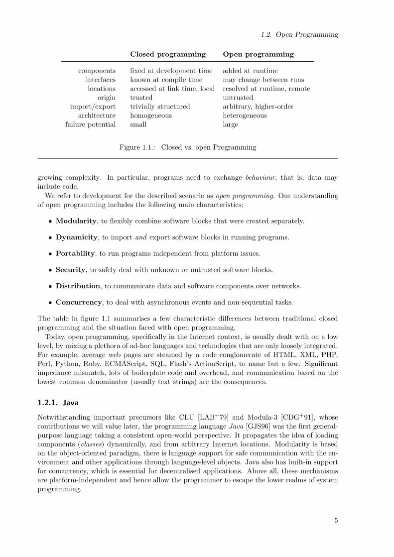
Closed programming Open programming
components fixed at development time added at runtimeinterfaces known at compile time may change between runslocations accessed at link time, local resolved at runtime, remote
origin trusted untrustedimport/export trivially structured arbitrary, higher-order
architecture homogeneous heterogeneousfailure potential small large
Figure 1.1.: Closed vs. open Programming
growing complexity. In particular, programs need to exchange behaviour, that is, data mayinclude code.
We refer to development for the described scenario as open programming. Our understandingof open programming includes the following main characteristics:
• Modularity, to flexibly combine software blocks that were created separately.
• Dynamicity, to import and export software blocks in running programs.
• Portability, to run programs independent from platform issues.
• Security, to safely deal with unknown or untrusted software blocks.
• Distribution, to communicate data and software components over networks.
• Concurrency, to deal with asynchronous events and non-sequential tasks.
The table in figure 1.1 summarises a few characteristic differences between traditional closedprogramming and the situation faced with open programming.
Today, open programming, specifically in the Internet context, is usually dealt with on a lowlevel, by mixing a plethora of ad-hoc languages and technologies that are only loosely integrated.For example, average web pages are steamed by a code conglomerate of HTML, XML, PHP,Perl, Python, Ruby, ECMAScript, SQL, Flash’s ActionScript, to name but a few. Significantimpedance mismatch, lots of boilerplate code and overhead, and communication based on thelowest common denominator (usually text strings) are the consequences.
1.2.1. Java
Notwithstanding important precursors like CLU [LAB+79] and Modula-3 [CDG+91], whosecontributions we will value later, the programming language Java [GJS96] was the first general-purpose language taking a consistent open-world perspective. It propagates the idea of loadingcomponents (classes) dynamically, and from arbitrary Internet locations. Modularity is basedon the object-oriented paradigm, there is language support for safe communication with the en-vironment and other applications through language-level objects. Java also has built-in supportfor concurrency, which is essential for decentralised applications. Above all, these mechanismsare platform-independent and hence allow the programmer to escape the lower realms of systemprogramming.
5
1. Introduction
As far as the programming language mainstream is concerned, Java heralded a shift ofparadigm: an application is no longer seen as a monolithic entity built from statically an-ticipated components, but as a dynamic service process that acquires additional components asthe need arises.
On the other hand, many of the open programming concepts found in Java are quite conser-vative and ad-hoc. In particular, its support for object exchange (serialisation) is comparablyprimitive and does not directly encompass higher-order use cases that would require transmissionof code. The Remote Method Invocation protocol, RMI [WRW96], and other such frameworkslater added to Java to address inter-process communication, work around this by transmittingclass files separately if not available at destination site. But since classes are identified only byname this is a rather fragile approach.
The most significant weakness of Java, however, and our main concern in the context of thisdissertation, is that its static type system is almost meaningless in the face of open programs,as we will discuss in Section 1.3.1.
1.2.2. Oz
While Java certainly has pioneered the open programming idea in the mainstream, moreresearch-oriented languages have carried it further, seeking for more expressive and more prin-cipled incarnations of the respective mechanisms. In particular, the concurrent constraint pro-gramming language Oz [Smo95, VH04, Moz04] has become an important platform for investi-gating and implementing related concepts in a practical context [DKSS98, Kor06].
Open programming in Oz is centered around generic support for pickling, which allows almostarbitrary values (including procedures and their code) to be imported and exported by processes.Based on pickling, Oz features a flexible component system with lazy dynamic linking, and richsupport for distributed programming. In particular, Oz pioneered the idea of representingcomponents as pickles.
The main omission of Oz is the lack of a static typing discipline. Oz has been designed as asafe but untyped language to enable free experimentation with new ideas. As the language hasstabilized, an obvious question is how to reconcile the evolved concepts with a type system. Inbrief, the practical part of our work is trying to give an answer to part of that question: in anutshell, it takes the essence of the open programming facilities found in Oz and developes atypeful counterpart. Alice ML also improves on Oz by increasing simplicity and regularity ofthe underlying concepts.
1.3. Typed Open Programming
The characteristics of open programming prevent full static type checking – at least some checkshave to be performed at runtime. For example, if a program loads an object from a file, thecompiler has no way of knowing in advance what actual type this object will have, since itusually will have been constructed outside the respective program.
In this light it is not surprising that the most advanced support for open programming can befound in “dynamically typed” languages, like Oz or Lisp/Scheme. These languages simply makeno assumptions about the type of anything, but instead perform dynamic checks every time anoperation is about to be performed that requires a value to have a certain shape. Consequently,the aforementioned problem does not arise.
It should be noted however, that this approach is no Silver Bullet for open programming. Someof the problems we will discuss exist in untyped languages as well. For example, unpickling isunsafe in the current implementation of Oz, despite its dynamic checks – the run-time system
6
1.3. Typed Open Programming
// Database.java, version 1class Database
Database(String path) ... public void lock() ... public void release() ... ...
// Database.java, version 2class Database
Database(String path) ... public void lock() ... public void unlock() ... ...
// App.javaclass App
public static void main(String[] args)
Database db = new Database(”/serve/my.db”);db.lock();// access data base...db.release();
Figure 1.2.: Dynamic typing in Java
cannot guarantee that loaded code is well-formed, for example, because that would again requiresome verification akin to type checking on the internal code format.
1.3.1. Java
When it comes to typed languages with support for open programming, the reference pointsurely is Java, which we already introduced in the previous section.
With respect to typing, Java is interesting because it uses a hybrid approach: it has a statictype system, but also performs run-time checks like “dynamically typed” languages. The reasonis that the type system actually is too weak to really encompass open programming: classtypes are essentially identified by their syntactic name only (more precisely, by name and classloader [LB98]), and no assumptions are checked about a class signature when it is loaded.Instead, checks are performed on individual method calls. That means that a class loaded atrun-time under the name C needs to bear no resemblance to the class found under the samename at compile time. In an open program, invocation of a method of C may thus potentiallyresult in a NoSuchMethodError or a related exception, i.e. a dynamic type error [LY96].
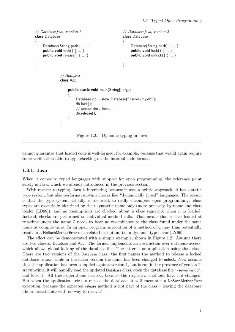
The effect can be demonstrated with a simple example, shown in Figure 1.2. Assume thereare two classes, Database and App. The former implements an abstraction over database access,which allows global locking of the database file. The latter is an application using that class.There are two versions of the Database class: the first names the method to release a lockeddatabase release, while in the latter version the name has been changed to unlock. Now assumethat the application has been compiled against version 1, but is run in the presence of version 2.At run-time, it will happily load the updated Database class, open the database file ”/serve/my.db”,and lock it. All these operations succeed, because the respective methods have not changed.But when the application tries to release the database, it will encounter a NoSuchMethodError
exception, because the expected release method is not part of the class – leaving the databasefile in locked state with no way to recover!
7
1. Introduction
The problem is that Java does not perform any structural check ensuring that App’s assump-tions about the Database class are still valid before allowing access to it. The checks are doneonly incrementally, but at that point it may already be too late. This is precisely the situationa type system should prevent.
Technically, Java’s type system may hence be considered unsound in the presence of open pro-gramming (although it is not unsafe – besides other dynamic checks, safety of dynamic loadingis ensured by a process called byte code verification). This lack of proper type soundness par-ticularly has ramifications on inter-process communication through serialisation (via persistenceor RMI): classes are identified by name, but there is no guarantee that different sites (or onesite at different times) actual use the same classes. Unexpected deserialisation failures may be aresult, or worse, values may successfully deserialise, but fail to meet semantic invariants of thelocal class implementation. In other words, Java cannot prevent accidental breach of abstractionsafety across process boundaries.
A simple but overly restrictive solution to this problem might be to hash class files witha cryptographic checksum. This would rule out incompatible changes to a class, but also allcompatible changes, i.e. simple interface extensions. In an open programming scenario suchinflexibility is not desirable.
1.3.2. Dynamics
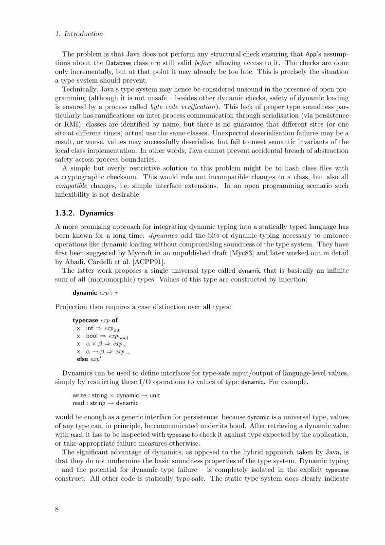
A more promising approach for integrating dynamic typing into a statically typed language hasbeen known for a long time: dynamics add the bits of dynamic typing necessary to embraceoperations like dynamic loading without compromising soundness of the type system. They havefirst been suggested by Mycroft in an unpublished draft [Myc83] and later worked out in detailby Abadi, Cardelli et al. [ACPP91].
The latter work proposes a single universal type called dynamic that is basically an infinitesum of all (monomorphic) types. Values of this type are constructed by injection:
dynamic exp : τ
Projection then requires a case distinction over all types:
typecase exp of
x : int ⇒ expint
x : bool ⇒ expbool
x : α× β ⇒ exp×
x : α→ β ⇒ exp→
else exp′
Dynamics can be used to define interfaces for type-safe input/output of language-level values,simply by restricting these I/O operations to values of type dynamic. For example,
write : string × dynamic → unitread : string → dynamic
would be enough as a generic interface for persistence: because dynamic is a universal type, valuesof any type can, in principle, be communicated under its hood. After retrieving a dynamic valuewith read, it has to be inspected with typecase to check it against type expected by the application,or take appropriate failure measures otherwise.
The significant advantage of dynamics, as opposed to the hybrid approach taken by Java, isthat they do not undermine the basic soundness properties of the type system. Dynamic typing– and the potential for dynamic type failure – is completely isolated in the explicit typecase
construct. All other code is statically type-safe. The static type system does clearly indicate
8
1.4. Contribution
where knowledge about the type of values is limited, by assigning type dynamic. The boundariesof static typing are thereby evident in a program.
There has been a range of follow-up work improving on dynamics, particularly by allowingpolymorphic content [LM93, ACPR95]. Later work has decoupled dynamic case switching ontypes by introducing type analysis as a stand-alone construct [HM95, CWM98, TSS00, Wei02],thereby allowing to reduce dynamics to values of existential type ∃α.α.
So, if everything is roses, why have dynamics not been widely adopted in typed programminglanguages? Our view is that there are two main problems with dynamics that have preventedtheir wide-spread adoption so far:
• Pragmatically, dynamics as proposed are too inconvenient for many applications. A gen-eral type case with the ability to handle polymorphism is complex and sometimes notstraightforward to use. More seriously, it is too fine-grained for the purpose of open pro-gramming, because it works on the granularity of single values. If one wants to transfera program component it is highly undesirable to require encoding its content in, say, asingle tuple value. Moreover, components may contain other entities than plain values,that cannot be directly stored in a value. Furthermore, type case is too inflexible to beused in evolving software systems, because the content type must be known very preciselyin order to unpack a dynamic. Subtyping would be very desirable, but raises coherenceissues in conjunction with a rich type case [ACPR95].
• Technically, the presence of dynamics (as well as general type analysis) destroys para-metricity [Rey83, BFSS89, ACC93], a valuable property of polymorphically typed lan-guages. Intuitively, parametricity means that an expression will always evaluate uniformly,no matter how any of its free types is instantiated, i.e. evaluation does not depend on types.That is a desirable abstraction property of polymorphism, for which Wadler coined theslogan “theorems for free” [Wad89]. For example, in plain polymorphic lambda calculus,a function of type ∀α.α → α is known to be the identity function. This is no longer truewith dynamics or more general forms of type analysis.
The loss of parametricity particularly affects the semantics of abstract types: in thestandard model of type abstraction, which is based on scoping of existential quantifi-cation [MP88], abstraction safety is lost because the representation of an abstract typecan be rediscovered dynamically, effectively allowing the definition of casts between ab-stract types and their representations. Lack of parametricity also has significant impacton the implementation and efficiency of a language: because types become part of theoperational semantics, they can no longer be erased, as it is done in almost all practicalimplementations of programming languages today. Instead, polymorphism requires a typepassing implementation.
Consequently, no practical programming language implements dynamics in their full beauty,nor does any seriously use it for open programming. Some languages, namely Clean [Pv00],Mercury [HCS+01], and the GHC implementation of Haskell [MPO02] incorporate simple vari-ants of dynamics, but except for Clean they make no use of it in their libraries. The GHCimplementation of dynamics even is unsafe, as it is not primitive but uses user-defined stringsto identify types.
1.4. Contribution
In this dissertation we develop a concrete and realistic language design for typed open pro-gramming. We focus on how typing interacts with open programming, primarily considering
9
1. Introduction
modularity and dynamicity. We also cover other aspects of open programming, like concurrencyand distribution, to a limited extent.
Our approach is based on the idea underlying dynamics, but does not suffer from the problemsdescribed above. In particular, it is easier for the programmer to understand and more convenientto use than dynamics. Furthermore, to reconcile it with type abstraction, we develop a semanticsfor type abstraction that is not compromised by the lack of parametricity.
In detail, our contributions are the following:
• We describe the design of a concrete, non-toy language, Alice ML, which is based onStandard ML [MTHM97], and incorporates a range of open programming features in acoherent way. It thus combines a particularly strong type system with flexible supportfor typed open programming. The presentation we give extends on previously publishedwork [RLT+06, Ros06].
• In particular, we introduce packages as a variation of dynamics that differ in that theycarry (potentially higher-order) modules instead of plain values. This allows to exchangearbitrary bundles of objects in convenient ways. When unpacked, a package is matchedagainst an expected interface in an intuitive manner already known from the modulesystem. Moreover, it implies a natural notion of interface inclusion that makes thesechecks robust against evolutionary changes.
• While we cannot avoid the loss of parametricity in principle, our language design confinesit to the module level – leaving parametricity intact for all uses of polymorphism occur-ring in the underlying core language. That maintains “theorems” where they are usuallyexploited, and allows for an efficient type erasing implementation.
• On top of packages and pickling we are able to define, as a layer of straightforward syntacticsugar, a powerful system of first-class components similar to what is found in Oz. Itsupports type-safe lazy dynamic linking, dynamic creation, and user-programmed linkingpolicies for security.
• We address the problem of abstraction safety (which still persists if parametricity is givenup for modules) by formulating a non-standard theory of abstract types in a calculus withdynamic generation of fresh type names instead of existential quantification. Unlike previ-ously published work [Ros03, Ros06], the calculus incorporates both type generation andtranslucency, expressed by singleton kinds, and hence captures the essentials of advancedmodule systems.
• The calculus employs coercions as a means of giving a reduction semantics for ADTs. Bygeneralising to higher-order coercions, we are able to recover the semantics of generativesealing for creating abstractions a posteriori, as it is common in module systems. Thecalculus seems to be the first that combines higher-order coercions with dependent andsingleton kinds, a combination that raises a number of technical difficulties.
• Our calculus also includes a simple but informative abstract semantics of pickling. Thatallows us to identify two independent forms of dynamic checking that have to be performedwhen unpickling.
• Our language design has been implemented in the Alice Programming System [Ali03],which is a full-scale programming environment available as open source software. Thesystem is being used in research and teaching.
10
1.5. Structure
Altogether, these contributions show that typed open programming is indeed possible, thussubstantiating our thesis. Because our approach even maintains abstraction safety across pro-cesses, we claim that it in fact enables typeful open programming (see Section 1.1.1). Moreover,we believe that the design of Alice ML is elegant and convenient enough to also make it suitableas a practical language for typed open programming, although a thorough evaluation of thatstronger claim lies beyond the scope of the thesis.
1.5. Structure
The rest of this dissertation will be split in two parts, developing our approach from two sides.In Part 1 we address the practical side and present and motivate the design of the concrete
programming language, Alice ML. We incrementally introduce the relevant language concepts,explaining their semantics informally, and demonstrating their use with concrete program ex-amples. The notion of component is introduced as derived syntax on the language level.
• Chapter 2 gives a brief overview of the features of Alice ML and its relation to the under-lying Standard ML (SML) programming language.
• Chapter 3 motivates and explains extensions to the SML module system.
• Chapter 4 introduces packages as the central means for dynamic typing.
• Chapter 5 describes pickling, the mechanism for importing and exporting higher-orderlanguage values.
• Chapter 6 introduces futures, enabling light-weight concurrency and lazy evaluation.
• Chapter 7 presents the dynamic component system, and describes its decomposition intoa combination of the concepts from the preceding chapters.
• Chapter 8 explains the language’s approach to distributed programming, which again isbased on the concepts previously introduced.
• Chapter 9 gives a brief overview of the implementation and discuss possible future workwith respect to language design and implementation.
In Part 2 we will cover the theoretical side by developing a formal calculus and type systemmodelling the essentials of this language. We distill the relevant concepts and put them into thecontext of a standard higher-order typed λ-calculus, for which we prove soundness properties aswell as a moderate abstraction result. In this calculus, we can define sealing as derived syntax.
• Chapter 10 introduces the λωSAΨ-calculus and motivates each of its features by relating it
to examples from Alice ML.
• Chapter 11 discusses the type language of the calculus, particularly the semantics of single-ton kinds and the novel notion of abstraction kinds, and gives various properties, includingdecidability.
• Chapter 12 discusses the term language and its operational semantics, with focus on dy-namic typing and type generation, and gives a soundness result and an abstraction propertywe call opacity.
• Chapter 13 extends the calculus with higher-order constructs to encompass higher-orderabstraction and shows how these constructs allow the encoding of higher-order sealing,which is proved correct.
• Chapter 14 concludes and discusses possible directions for future work.
At the end of each chapter we discuss prior work related to the topic of the respective chapter.
11

1. Introduction
12
Part I.
Introducing Alice ML
13

2. Overview
The following chapters provide an overview of the functional programming language Alice ML.Alice ML has been specifically designed to support typed open programming. It extends theconventional feature set of functional languages with a novel combination of concepts supportingconcurrency, distribution, and particularly, type-safe import and export of program components– that is, typed open programming. We present the central concepts of Alice ML, motivatethem with examples, and show how they play together as a coherent whole.
This presentation is not intended to be a language specification. We keep the descriptioninformal and concentrate on the essentials of the semantics. Theoretic considerations are left tothe second and third part of this thesis, where we look at a more idealised language that lendsitself better to theoretic study. A formal specification of a significant subset of Alice ML is givenin a technical report [Ros05].
The material in this part of the thesis extends on previously published work describing aspectsof the design of Alice ML [RLT+06, Ros06]. We will discuss it along with other related work atthe end of each chapter.
To warm up, we start off in this chapter by giving a brief recap of Standard ML, on whichAlice ML is based, and summarise the extensions that Alice ML provides. We also introduce theAlice Programming System [Ali03], that implements the Alice ML language. In the followingchapters we then present the key concepts of Alice ML in more detail: higher-order modules(Chapter 3), dynamic typing with packages (Chapter 4), high-level import/export with pickling(Chapter 5), concurrency with futures (Chapter 6), the component system (Chapter 7), anddistributed programming (Chapter 8). On the way, we introduce many of the open programmingfacilities provided by the Alice library, which make use of all the aforementioned concepts.
2.1. Standard ML Heritage
Alice ML is a functional programming language in the tradition of ML, a family of typedfunctional languages with pragmatic support for imperative programming. Alice ML has beendesigned as a mostly conservative extension of the ML incarnation known as Standard ML[MTHM97], or simply SML.
ML was originally developed in the late 1970s by Milner as a Meta Language for the LCFproof-checking system [GMW79]. Over the years, its development brought three major innova-tions to the field of programming languages: the introduction of polymorphic typing with typeinference [Mil78, DM82] (the same idea already had been discovered earlier in the context of com-binatory logic [Hin69]), a parametric module system based on dependent types [Mac86, Mac84],and rigorous formal specification of a complete language, the Definition of Standard ML[MTH90, MTHM97].
Today, there are several implementations of Standard ML, plus a major dialect called Ob-jective Caml [Ler03], which particularly adds a rich object-oriented sublanguage. ML enjoys aprominent position in language research and teaching, thanks to its clean design and specifica-tion, and the expressive yet robust higher-order semantics. The main features of the ML familyof languages as of today can be summarized as follows:
15
2. Overview
• Functional core. A higher-order functional language with a strict evaluation regimeconstitutes the core language.
• Imperative features. Besides a pure functional subset, imperative constructs like ex-ception handling and mutable references are available.
• Algebraic data types. User-defined data types come with a concise notation for patternmatching.
• Polymorphic type system. A strong static type system provides parametric polymor-phism and supports type inference.
• Parametric module system. The module system is a functional language on its own,with strong support for encapsulation and parameterisation.
• Safe semantics. No program can ever “go wrong”, i.e. access computational resourcesin an invalid or unsafe way.
Due to its clean formal specification, SML is a particularly well suited vehicle for programminglanguage research. Its comparatively expressive and well-studied type and module system is agood match for exploring typed open programming. Consequently, Alice ML has been designedas a conservative extension to the revised version of Standard ML, with some ideas borrowedfrom Objective Caml.
Giving an introduction to Standard ML, or to functional programming in general, is out ofthe scope of this work. We refer the interested reader to the available literature [Har06, Pau96,Ull97, HR99]. In the following, we assume a working knowledge of SML, or some other dialectof the ML family of languages. Where important, we will briefly summarize central concepts ofSML alongside our presentation of Alice ML.
2.2. Extensions and Oz Heritage
Alice ML has been designed as a conservative extension of SML. Most SML programs can bereadily interpreted as Alice ML programs. However, while Alice ML is backward compatiblewith SML, it also features significant extensions:
• Futures. A future is a place-holder for a yet undetermined value, usually computed by aconcurrent thread. Different flavours of futures provide laziness, light-weight concurrency,and promises, a restricted form of logic variable.
• Higher-order modules. Structures, functors, and signatures can be defined locally andcomposed arbitrarily. In particular, signatures can contain signature members, and liketypes, these may be abstract or concrete.
• Packages. Modules may be passed as dynamically typed first-class values by injectingthem into a special type known as package. A package value carries information about thecontained module’s signature. When accessing the package, the signature is verified bya dynamic type check. Packages are the basis for type-safe persistence and distribution.Thanks to higher-order modules, packages can contain arbitrary language entities.
• Pickling. A generic mechanism for import and export of language-level data structures,including code. A pickle is a self-contained, platform-independent external representationof an Alice ML value. The library interface to pickling is type-safe because it operates onpackages.
16
2.3. The Alice Programming System
• Components. Programs are decomposed into separate components that are connectedvia import relations. Linking of imported components is performed dynamically and ona by-need basis, and involves dynamic verification of signature assumptions. Componentsare expressed in terms of packages, pickling and lazy futures.
• Distribution. Alice processes on different sites can connect to each other and safelyexchange almost arbitrary Alice data structures. Processes may create proxies to localfunctions that, when applied, transparently perform a remote procedure call to the orig-inal process. Futures play an important role to deal with asynchronicity and latency indistributed programming.
Each of these concepts is realised by augmenting the basic language with only a few simple andorthogonal, yet general and powerful constructs. These constructs extend the semantics of theoriginal language in considerable ways, while maintaining most of its valuable properties.
Most of the features specifically targeting open programming – i.e. pickling, components anddistribution – are inherited in one form or another from the concurrent constraint programminglanguage Oz [Smo95, VH04, DKSS98, Moz04]. We will discuss the relation where appropriate.
Packages and a strongly typed model of components are the primary features that are novelto Alice ML and the main concern of this thesis. In the following chapters, we will introduce andmotivate all of the above features, because they all play together to enable open programming.But because the design of packages and components is the main contribution of this thesis, wewill particularly focus on packages and components and the issues with dynamic typing thatthey address.
2.3. The Alice Programming System
Alice ML has been implemented in a fully-featured programming system [Ali03]. Having athand not only a toy implementation, but a fully-featured prototype that allows playing with thelanguage under realistic conditions, proved immensely helpful during the design of Alice ML. TheAlice System provides a compiler for the full language, an efficient platform-independent virtualmachine with support for distributed programming, several interactive development tools, andextensive libraries.
Another central feature of the Alice Programming System is its rich support for constraintprogramming [Apt03, Sch02], based on the Gecode constraint programming library [Gec05,ST05]. Since constraint programming in Alice ML is purely a library issue and does not requirespecial language support we will not discuss that aspect of Alice further in this thesis. We referthe reader to the Alice documentation [Ali03] for details.
The first pre-version of Alice (still based on the Mozart Programming System [Moz04]) wasreleased in December 2002. The official 1.0 release of Alice followed in 2004, and there havebeen regular updates since. The Alice Programming System is freely available as open sourcesoftware, and runs on all major platforms.
2.4. Summary
• Alice ML is a language designed for typed open programming.
• It is a mostly conservative extension of Standard ML.
17
2. Overview
• Notable extensions are future-based concurrency and laziness, higher-order modules, dy-namically typed modules (packages), pickling, components, and distributed programmingfeatures.
• Alice ML has been fully implemented in the Alice Programming System, which is availableas open source software.
18
3. Higher-Order Modules
Large-scale programming requires the ability to break down the complexity of programs, andto avoid duplicating work for different programs or different parts of a single program. Hence,modules allow the decomposition of programs into units that implement dedicated aspects of itslogic and functionality. They particularly support the definition of abstractions, which reducescoupling and increases the potential for re-use in different contexts.
Modules thus play a central role in structuring ML programs. The ML module system stilldefines the state-of-the-art in language design for typed modular programming. The followingis a brief summary of the main features of the SML module system:
• Structures are the basic form of module. They are containers that can carry arbitrary corelanguage entities, like values and types, as well as nested structures. Structure membersare named and can be accessed by dot notation.
• Signatures are the types of structures. They describe the members of a structure. Signa-tures are translucent, that is, types can be described either concretely (transparent, mani-fest) or abstractly (opaque). In the former case, the type equivalence is revealed, while inthe latter it is not. Every structure has a principal signature that is fully concrete.1
• Matching is subtyping on signatures. The subtyping relation consists of two dimensions:enrichment allows a subsignature to extend a supersignature with additional members;instantiation allows a subsignature to concretise types that are abstract in the supersig-nature. The signature language contains syntax for refining a given signature along bothdimensions.
• Sealing is an operation that ascribes a signature to a structure, using the syntax strexp:> sigexp. The identity of any type described abstractly in the signature is thereby hiddenoutside the sealed structure. Sealing is said to be generative, because it effectively generatesnew abstract types that are distinct from all others.
• Functors are (first-order) functions over structures. By applying a functor to a structurea new structure is computed whose content and signature can depend on the suppliedargument. Functors are also said to be generative, because applying the same functortwice to the same argument produces distinct abstract types, if the functor returns asealed structure.
• Stratification describes the fact that the module language is completely separated fromthe core language. Core language expressions cannot contain module expressions anddeclarations. Modules are solely a means for structuring large programs and describingprogram architectures.
When it comes to open programming, good language support for modularity is essential. TheSML module system is quite advanced in comparison to most other languages, but still limitedby its restriction to first-order parameterisation and its stratified setup. Since the design of
1Although not all principal signatures are expressible in the surface syntax.
19
3. Higher-Order Modules
the original SML module system there has been a long line of work on extending its expressivepower (Section 3.4). Alice ML integrates some of that work by extending the module system ofSML in three ways:
• Higher-order functors. Functors can be arbitrarily nested and parameterised over otherfunctors.
• Nested and abstract signatures. Signatures can be wrapped in structures and bespecified abstractly.
• Local modules. Modules can be defined within core let expressions.
These extensions allow new and more flexible forms of abstraction. Modular techniques areapplicable at more fine-grained levels, which is particularly important for dealing with pack-ages (Chapter 4). Simultaneously, the extensions generalise the module language such that itis rendered more regular and compositional than in plain SML. Most importantly, structuresbecome a general container that can carry all sorts of language entities (values, types, modules,signatures, even fixity directives). Again, this is crucial to the expressive power of packages, andit is essential to the design of the Alice component system (Chapter 7).
Higher-order modules are neither new nor exclusive to Alice ML. Consequently, this chapteronly gives some motivation for adding them and an overview of their specific design in Al-ice ML. Their semantics and theoretical underpinnings have been investigated extensively inliterature [HMM90, MT94, HL94, Ler95, DCH03, Rus98].
3.1. Higher-Order Functors
The module language of Standard ML is first-order: functors can take structures as argumentsand return structures as results, but they cannot accept or return other functors. Neither canfunctors be put into structures. The first-order restriction on functors can sometimes hampermodular design, even without the particular requirements of open programming.
Consider a conventional example: a compiler that consists of several phases (stages). Eachphase translates one intermediate program representation into another one, using some contex-tual information. A suitable signature for describing a compiler phase might be the following:
signature PHASE =sig
type in reptype out reptype contextval translate : context → in rep → out rep
end
A compiler is essentially a pipe of different phases. To construct it, we need a way to plug phasestogether. We can achieve this by repeatedly applying a functor for composing two consecutivephases:2
functor ComposePhases(structure Phase1 : PHASEstructure Phase2 : PHASE where type in rep = Phase1.out rep) =
struct
type in rep = Phase1.in rep
2The Alice ML compiler itself is constructed this way.
20
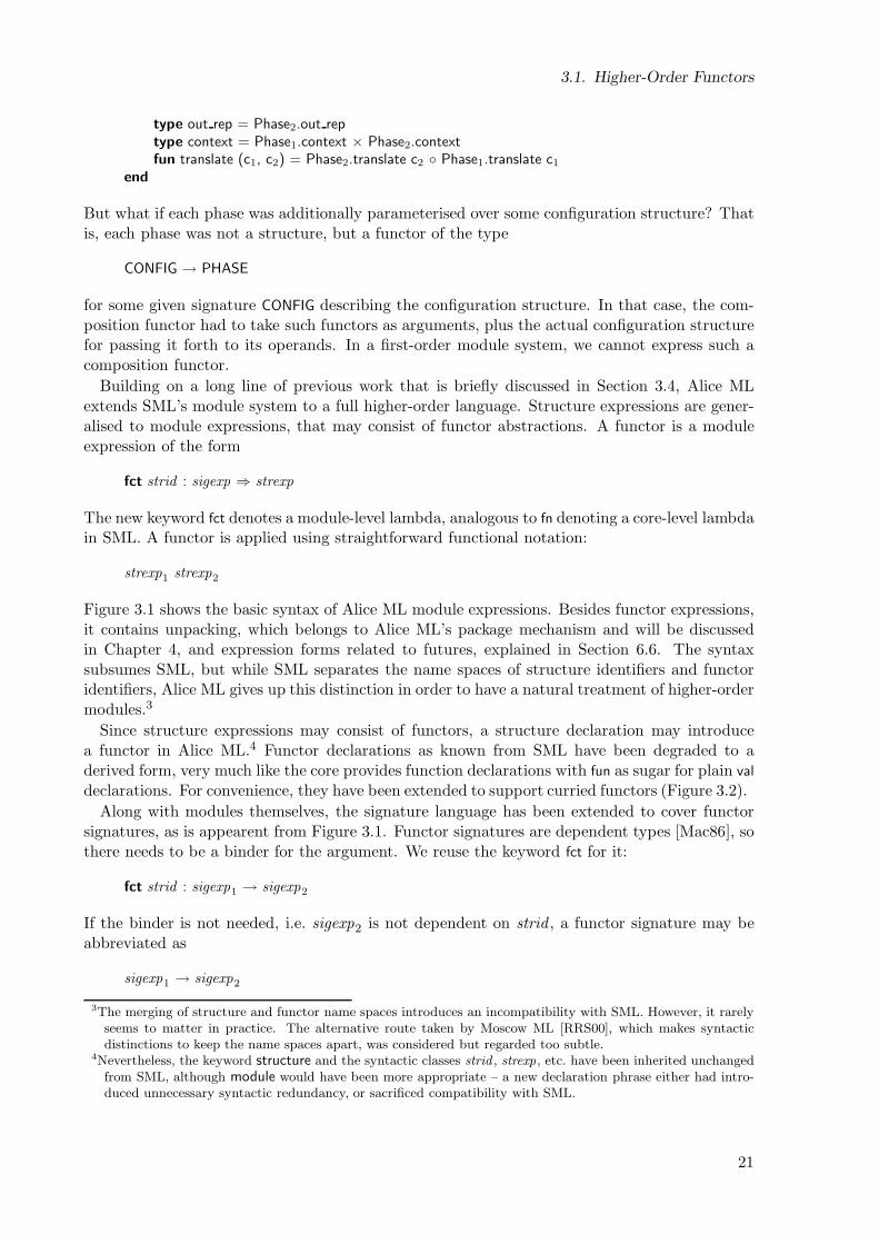
3.1. Higher-Order Functors
type out rep = Phase2.out reptype context = Phase1.context × Phase2.contextfun translate (c1, c2) = Phase2.translate c2 Phase1.translate c1
end
But what if each phase was additionally parameterised over some configuration structure? Thatis, each phase was not a structure, but a functor of the type
CONFIG → PHASE
for some given signature CONFIG describing the configuration structure. In that case, the com-position functor had to take such functors as arguments, plus the actual configuration structurefor passing it forth to its operands. In a first-order module system, we cannot express such acomposition functor.
Building on a long line of previous work that is briefly discussed in Section 3.4, Alice MLextends SML’s module system to a full higher-order language. Structure expressions are gener-alised to module expressions, that may consist of functor abstractions. A functor is a moduleexpression of the form
fct strid : sigexp ⇒ strexp
The new keyword fct denotes a module-level lambda, analogous to fn denoting a core-level lambdain SML. A functor is applied using straightforward functional notation:
strexp1 strexp2
Figure 3.1 shows the basic syntax of Alice ML module expressions. Besides functor expressions,it contains unpacking, which belongs to Alice ML’s package mechanism and will be discussedin Chapter 4, and expression forms related to futures, explained in Section 6.6. The syntaxsubsumes SML, but while SML separates the name spaces of structure identifiers and functoridentifiers, Alice ML gives up this distinction in order to have a natural treatment of higher-ordermodules.3
Since structure expressions may consist of functors, a structure declaration may introducea functor in Alice ML.4 Functor declarations as known from SML have been degraded to aderived form, very much like the core provides function declarations with fun as sugar for plain val
declarations. For convenience, they have been extended to support curried functors (Figure 3.2).
Along with modules themselves, the signature language has been extended to cover functorsignatures, as is appearent from Figure 3.1. Functor signatures are dependent types [Mac86], sothere needs to be a binder for the argument. We reuse the keyword fct for it:
fct strid : sigexp1 → sigexp2
If the binder is not needed, i.e. sigexp2 is not dependent on strid , a functor signature may beabbreviated as
sigexp1 → sigexp2
3The merging of structure and functor name spaces introduces an incompatibility with SML. However, it rarelyseems to matter in practice. The alternative route taken by Moscow ML [RRS00], which makes syntacticdistinctions to keep the name spaces apart, was considered but regarded too subtle.
4Nevertheless, the keyword structure and the syntactic classes strid , strexp, etc. have been inherited unchangedfrom SML, although module would have been more appropriate – a new declaration phrase either had intro-duced unnecessary syntactic redundancy, or sacrificed compatibility with SML.
21
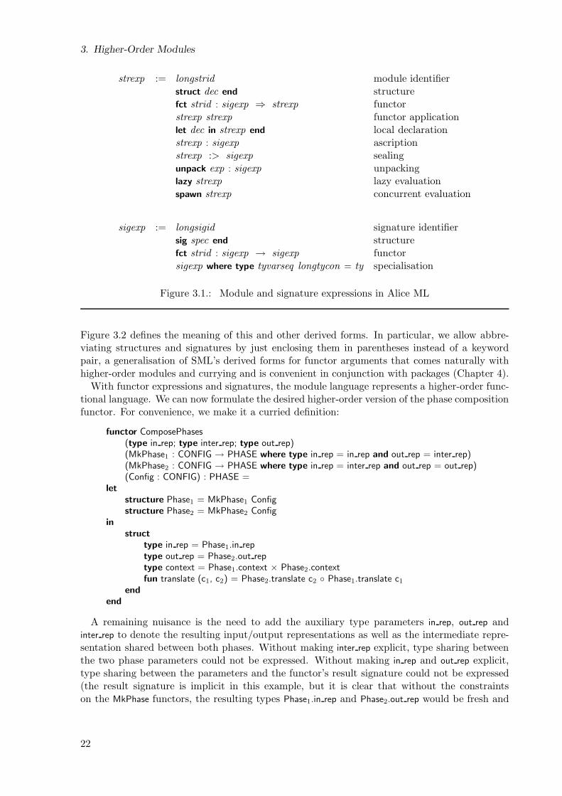
3. Higher-Order Modules
strexp := longstrid module identifierstruct dec end structurefct strid : sigexp ⇒ strexp functorstrexp strexp functor applicationlet dec in strexp end local declarationstrexp : sigexp ascriptionstrexp :> sigexp sealingunpack exp : sigexp unpackinglazy strexp lazy evaluationspawn strexp concurrent evaluation
sigexp := longsigid signature identifiersig spec end structurefct strid : sigexp → sigexp functorsigexp where type tyvarseq longtycon = ty specialisation
Figure 3.1.: Module and signature expressions in Alice ML
Figure 3.2 defines the meaning of this and other derived forms. In particular, we allow abbre-viating structures and signatures by just enclosing them in parentheses instead of a keywordpair, a generalisation of SML’s derived forms for functor arguments that comes naturally withhigher-order modules and currying and is convenient in conjunction with packages (Chapter 4).
With functor expressions and signatures, the module language represents a higher-order func-tional language. We can now formulate the desired higher-order version of the phase compositionfunctor. For convenience, we make it a curried definition:
functor ComposePhases(type in rep; type inter rep; type out rep)(MkPhase1 : CONFIG → PHASE where type in rep = in rep and out rep = inter rep)(MkPhase2 : CONFIG → PHASE where type in rep = inter rep and out rep = out rep)(Config : CONFIG) : PHASE =
let
structure Phase1 = MkPhase1 Configstructure Phase2 = MkPhase2 Config
in
struct
type in rep = Phase1.in reptype out rep = Phase2.out reptype context = Phase1.context × Phase2.contextfun translate (c1, c2) = Phase2.translate c2 Phase1.translate c1
end
end
A remaining nuisance is the need to add the auxiliary type parameters in rep, out rep andinter rep to denote the resulting input/output representations as well as the intermediate repre-sentation shared between both phases. Without making inter rep explicit, type sharing betweenthe two phase parameters could not be expressed. Without making in rep and out rep explicit,type sharing between the parameters and the functor’s result signature could not be expressed(the result signature is implicit in this example, but it is clear that without the constraintson the MkPhase functors, the resulting types Phase1.in rep and Phase2.out rep would be fresh and
22
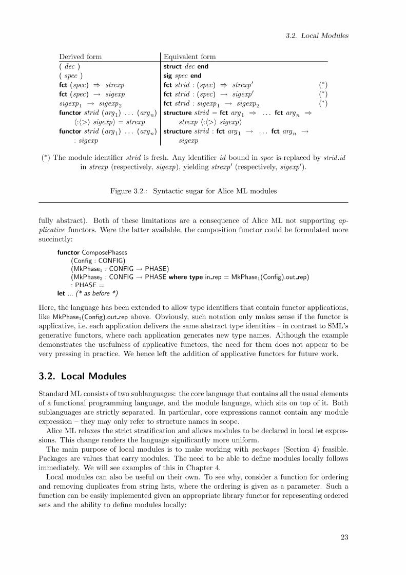
3.2. Local Modules
Derived form Equivalent form
( dec ) struct dec end
( spec ) sig spec end
fct (spec) ⇒ strexp fct strid : (spec) ⇒ strexp ′ (∗)fct (spec) → sigexp fct strid : (spec) → sigexp′ (∗)sigexp1 → sigexp2 fct strid : sigexp1 → sigexp2 (∗)functor strid (arg1) . . . (argn) structure strid = fct arg1 ⇒ . . . fct argn ⇒
〈:〈>〉 sigexp〉 = strexp strexp 〈:〈>〉 sigexp〉functor strid (arg1) . . . (argn) structure strid : fct arg1 → . . . fct argn →
: sigexp sigexp
(∗) The module identifier strid is fresh. Any identifier id bound in spec is replaced by strid .id
in strexp (respectively, sigexp), yielding strexp ′ (respectively, sigexp′).
Figure 3.2.: Syntactic sugar for Alice ML modules
fully abstract). Both of these limitations are a consequence of Alice ML not supporting ap-plicative functors. Were the latter available, the composition functor could be formulated moresuccinctly:
functor ComposePhases(Config : CONFIG)(MkPhase1 : CONFIG → PHASE)(MkPhase2 : CONFIG → PHASE where type in rep = MkPhase1(Config).out rep): PHASE =
let ... (* as before *)
Here, the language has been extended to allow type identifiers that contain functor applications,like MkPhase1(Config).out rep above. Obviously, such notation only makes sense if the functor isapplicative, i.e. each application delivers the same abstract type identities – in contrast to SML’sgenerative functors, where each application generates new type names. Although the exampledemonstrates the usefulness of applicative functors, the need for them does not appear to bevery pressing in practice. We hence left the addition of applicative functors for future work.
3.2. Local Modules
Standard ML consists of two sublanguages: the core language that contains all the usual elementsof a functional programming language, and the module language, which sits on top of it. Bothsublanguages are strictly separated. In particular, core expressions cannot contain any moduleexpression – they may only refer to structure names in scope.
Alice ML relaxes the strict stratification and allows modules to be declared in local let expres-sions. This change renders the language significantly more uniform.
The main purpose of local modules is to make working with packages (Section 4) feasible.Packages are values that carry modules. The need to be able to define modules locally followsimmediately. We will see examples of this in Chapter 4.
Local modules can also be useful on their own. To see why, consider a function for orderingand removing duplicates from string lists, where the ordering is given as a parameter. Such afunction can be easily implemented given an appropriate library functor for representing orderedsets and the ability to define modules locally:
23
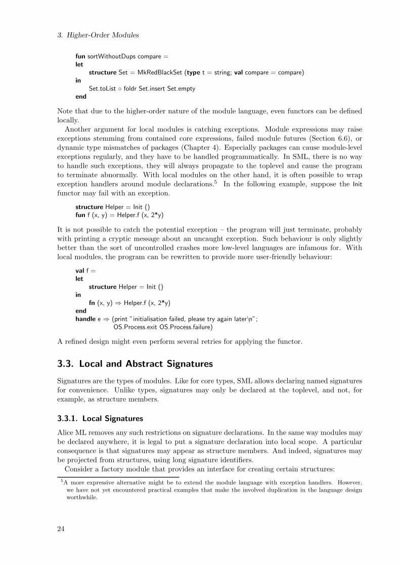
3. Higher-Order Modules
fun sortWithoutDups compare =let
structure Set = MkRedBlackSet (type t = string; val compare = compare)in
Set.toList foldr Set.insert Set.emptyend
Note that due to the higher-order nature of the module language, even functors can be definedlocally.
Another argument for local modules is catching exceptions. Module expressions may raiseexceptions stemming from contained core expressions, failed module futures (Section 6.6), ordynamic type mismatches of packages (Chapter 4). Especially packages can cause module-levelexceptions regularly, and they have to be handled programmatically. In SML, there is no wayto handle such exceptions, they will always propagate to the toplevel and cause the programto terminate abnormally. With local modules on the other hand, it is often possible to wrapexception handlers around module declarations.5 In the following example, suppose the Init
functor may fail with an exception.
structure Helper = Init ()fun f (x, y) = Helper.f (x, 2*y)
It is not possible to catch the potential exception – the program will just terminate, probablywith printing a cryptic message about an uncaught exception. Such behaviour is only slightlybetter than the sort of uncontrolled crashes more low-level languages are infamous for. Withlocal modules, the program can be rewritten to provide more user-friendly behaviour:
val f =let
structure Helper = Init ()in
fn (x, y) ⇒ Helper.f (x, 2*y)end
handle e ⇒ (print ”initialisation failed, please try again later\n”;OS.Process.exit OS.Process.failure)
A refined design might even perform several retries for applying the functor.
3.3. Local and Abstract Signatures
Signatures are the types of modules. Like for core types, SML allows declaring named signaturesfor convenience. Unlike types, signatures may only be declared at the toplevel, and not, forexample, as structure members.
3.3.1. Local Signatures
Alice ML removes any such restrictions on signature declarations. In the same way modules maybe declared anywhere, it is legal to put a signature declaration into local scope. A particularconsequence is that signatures may appear as structure members. And indeed, signatures maybe projected from structures, using long signature identifiers.
Consider a factory module that provides an interface for creating certain structures:
5A more expressive alternative might be to extend the module language with exception handlers. However,we have not yet encountered practical examples that make the involved duplication in the language designworthwhile.
24
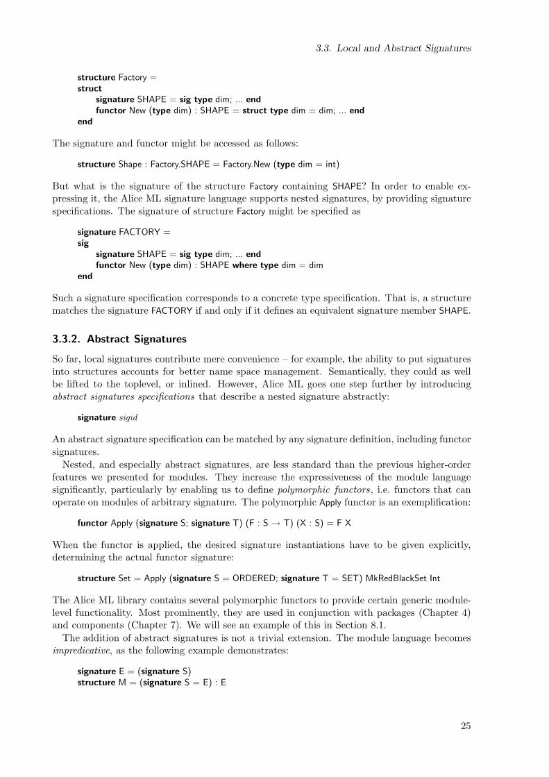
3.3. Local and Abstract Signatures
structure Factory =struct
signature SHAPE = sig type dim; ... end
functor New (type dim) : SHAPE = struct type dim = dim; ... end
end
The signature and functor might be accessed as follows:
structure Shape : Factory.SHAPE = Factory.New (type dim = int)
But what is the signature of the structure Factory containing SHAPE? In order to enable ex-pressing it, the Alice ML signature language supports nested signatures, by providing signaturespecifications. The signature of structure Factory might be specified as
signature FACTORY =sig
signature SHAPE = sig type dim; ... end
functor New (type dim) : SHAPE where type dim = dimend
Such a signature specification corresponds to a concrete type specification. That is, a structurematches the signature FACTORY if and only if it defines an equivalent signature member SHAPE.
3.3.2. Abstract Signatures
So far, local signatures contribute mere convenience – for example, the ability to put signaturesinto structures accounts for better name space management. Semantically, they could as wellbe lifted to the toplevel, or inlined. However, Alice ML goes one step further by introducingabstract signatures specifications that describe a nested signature abstractly:
signature sigid
An abstract signature specification can be matched by any signature definition, including functorsignatures.
Nested, and especially abstract signatures, are less standard than the previous higher-orderfeatures we presented for modules. They increase the expressiveness of the module languagesignificantly, particularly by enabling us to define polymorphic functors, i.e. functors that canoperate on modules of arbitrary signature. The polymorphic Apply functor is an exemplification:
functor Apply (signature S; signature T) (F : S → T) (X : S) = F X
When the functor is applied, the desired signature instantiations have to be given explicitly,determining the actual functor signature:
structure Set = Apply (signature S = ORDERED; signature T = SET) MkRedBlackSet Int
The Alice ML library contains several polymorphic functors to provide certain generic module-level functionality. Most prominently, they are used in conjunction with packages (Chapter 4)and components (Chapter 7). We will see an example of this in Section 8.1.
The addition of abstract signatures is not a trivial extension. The module language becomesimpredicative, as the following example demonstrates:
signature E = (signature S)structure M = (signature S = E) : E
25
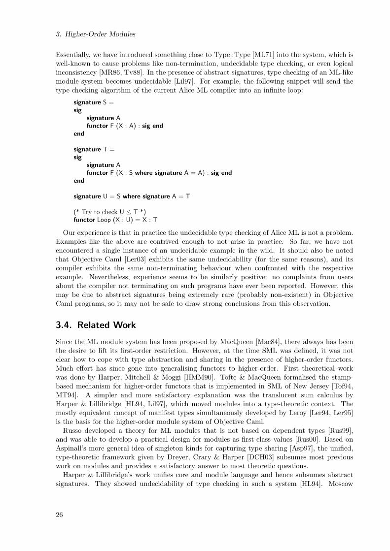
3. Higher-Order Modules
Essentially, we have introduced something close to Type : Type [ML71] into the system, which iswell-known to cause problems like non-termination, undecidable type checking, or even logicalinconsistency [MR86, Tv88]. In the presence of abstract signatures, type checking of an ML-likemodule system becomes undecidable [Lil97]. For example, the following snippet will send thetype checking algorithm of the current Alice ML compiler into an infinite loop:
signature S =sig
signature Afunctor F (X : A) : sig end
end
signature T =sig
signature Afunctor F (X : S where signature A = A) : sig end
end
signature U = S where signature A = T
(* Try to check U ≤ T *)functor Loop (X : U) = X : T
Our experience is that in practice the undecidable type checking of Alice ML is not a problem.Examples like the above are contrived enough to not arise in practice. So far, we have notencountered a single instance of an undecidable example in the wild. It should also be notedthat Objective Caml [Ler03] exhibits the same undecidability (for the same reasons), and itscompiler exhibits the same non-terminating behaviour when confronted with the respectiveexample. Nevertheless, experience seems to be similarly positive: no complaints from usersabout the compiler not terminating on such programs have ever been reported. However, thismay be due to abstract signatures being extremely rare (probably non-existent) in ObjectiveCaml programs, so it may not be safe to draw strong conclusions from this observation.
3.4. Related Work
Since the ML module system has been proposed by MacQueen [Mac84], there always has beenthe desire to lift its first-order restriction. However, at the time SML was defined, it was notclear how to cope with type abstraction and sharing in the presence of higher-order functors.Much effort has since gone into generalising functors to higher-order. First theoretical workwas done by Harper, Mitchell & Moggi [HMM90]. Tofte & MacQueen formalised the stamp-based mechanism for higher-order functors that is implemented in SML of New Jersey [Tof94,MT94]. A simpler and more satisfactory explanation was the translucent sum calculus byHarper & Lillibridge [HL94, Lil97], which moved modules into a type-theoretic context. Themostly equivalent concept of manifest types simultaneously developed by Leroy [Ler94, Ler95]is the basis for the higher-order module system of Objective Caml.
Russo developed a theory for ML modules that is not based on dependent types [Rus99],and was able to develop a practical design for modules as first-class values [Rus00]. Based onAspinall’s more general idea of singleton kinds for capturing type sharing [Asp97], the unified,type-theoretic framework given by Dreyer, Crary & Harper [DCH03] subsumes most previouswork on modules and provides a satisfactory answer to most theoretic questions.
Harper & Lillibridge’s work unifies core and module language and hence subsumes abstractsignatures. They showed undecidability of type checking in such a system [HL94]. Moscow
26
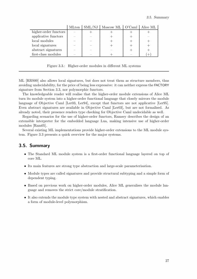
3.5. Summary
MLton SML/NJ Moscow ML O’Caml Alice ML
higher-order functors – + + + +applicative functors – – + + –local modules – – + + +local signatures – – + + +abstract signatures – – – + +first-class modules – – + – (+)
Figure 3.3.: Higher-order modules in different ML systems
ML [RRS00] also allows local signatures, but does not treat them as structure members, thusavoiding undecidability, for the price of being less expressive: it can neither express the FACTORY
signature from Section 3.3, nor polymorphic functors.The knowledgeable reader will realise that the higher-order module extensions of Alice ML
turn its module system into a higher-order functional language that closely mirrors the modulelanguage of Objective Caml [Ler03, Ler94], except that functors are not applicative [Ler95].Even abstract signatures are available in Objective Caml [Ler03], but are not formalised. Asalready noted, their presence renders type checking for Objective Caml undecidable as well.
Regarding scenarios for the use of higher-order functors, Ramsey describes the design of anextensible interpreter for the embedded language Lua, making intensive use of higher-ordermodules [Ram05].
Several existing ML implementations provide higher-order extensions to the ML module sys-tem. Figure 3.3 presents a quick overview for the major systems.
3.5. Summary
• The Standard ML module system is a first-order functional language layered on top ofcore ML.
• Its main features are strong type abstraction and large-scale parameterisation.
• Module types are called signatures and provide structural subtyping and a simple form ofdependent typing.
• Based on previous work on higher-order modules, Alice ML generalises the module lan-guage and removes the strict core/module stratification.
• It also extends the module type system with nested and abstract signatures, which enablesa form of module-level polymorphism.
27

3. Higher-Order Modules
28
4. Packages
ML style modules are an indispensable aid for large-scale programming, thanks to their abilityto express complex modular abstractions. They provide namespacing, encapsulation, genericity,and architectural configuration in form of a small higher-order language with an expressive,strong type system. Higher-order modules even provide a semantic and linguistic foundation fornon-trivial architectural programming, or programming-in-the-large.
However, all this expressive power is purely static: a program has to be a closed moduleexpression. That is, the program must be determined and provided in its entirety at compiletime, prior to running it (compile time may include static linking steps). The program’s moduleexpressions could actually be evaluated at compile time1, and some implementations of StandardML in fact do that [Els99]. Once built, configuration, functionality, and extent of a conventionalML program is fixed – in other words, programs are closed. This situation is at odds with theopen programming scenario discussed in Section 1.2, where we identified the need to acquireprogram components dynamically, without them necessarily being available, or even anticipated,in advance. The ML module language provides nothing to address that need. Obviously, someadditional amount of dynamism is required, including the ability to defer some type checking toruntime – in other words, we need some form of dynamic typing.
Alice ML employs the novel notion of package to resolve this tension. Packages complementthe static module and type system of SML with the necessary amount of dynamic typing to gainthe desired dynamic flexibility, while not compromising any of the advantages of static typing.More precisely, they add two important capabilities to the language:
• Dynamic typing. The static type system is complemented with a flexible, controlledform of dynamic typing.
• Modules as first-class values. Modules can be encapsulated as first-class values, en-abling computations over modules.
Although this represents quite a dramatic change to the expressivity of the language, packagescome with the following properties:
• Type safety. Soundness and abstraction properties of the static type system are notcompromised.
• Economic design. Minimal conceptual overhead through maximal conceptual re-use.
• Idiomatic use. Well-understood idioms for module programming apply unchanged.
The package concept is a variation of the well-known idea of dynamics [ACPP91, LM93,ACPR95, Dug99]. The main difference is that they carry modules instead of plain values.As a consequence, they can reuse the module system’s flexible subtyping relation for dynamictype checking, instead of necessitating a complicated typecase construct for matching types.
The presence of packages has severe implications on other aspects of the language. A closelyrelated but more technical contribution of our work on Alice ML hence is a refined semantics
1Local modules as available in Alice ML (Section 3.2) generally cannot be evaluated statically, though.
29
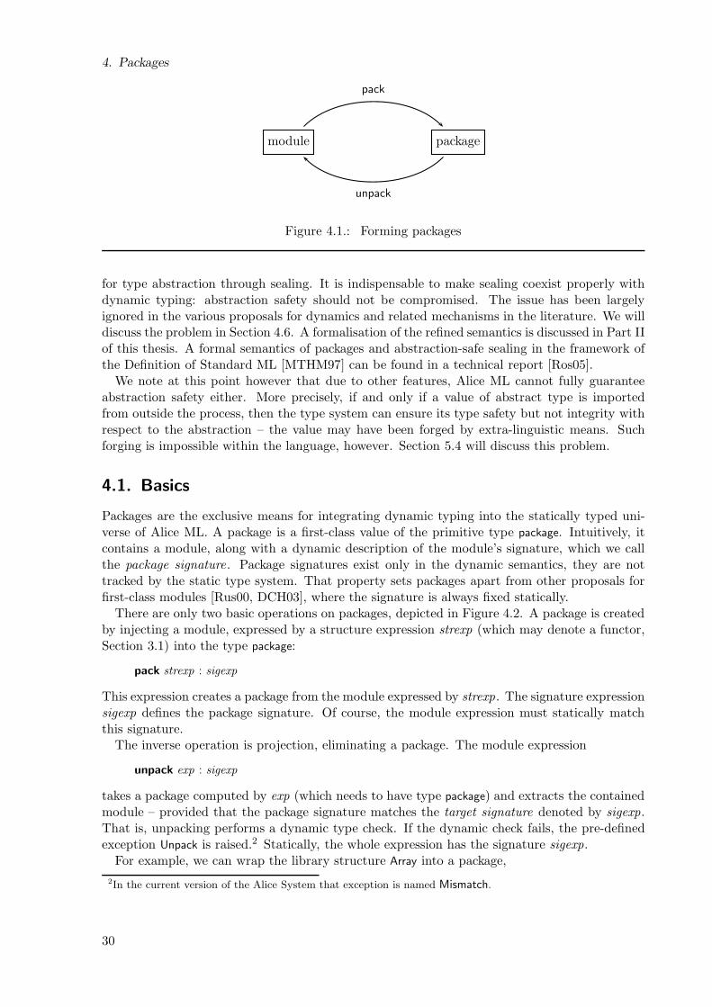
4. Packages
module package
pack
unpack
Figure 4.1.: Forming packages
for type abstraction through sealing. It is indispensable to make sealing coexist properly withdynamic typing: abstraction safety should not be compromised. The issue has been largelyignored in the various proposals for dynamics and related mechanisms in the literature. We willdiscuss the problem in Section 4.6. A formalisation of the refined semantics is discussed in Part IIof this thesis. A formal semantics of packages and abstraction-safe sealing in the framework ofthe Definition of Standard ML [MTHM97] can be found in a technical report [Ros05].
We note at this point however that due to other features, Alice ML cannot fully guaranteeabstraction safety either. More precisely, if and only if a value of abstract type is importedfrom outside the process, then the type system can ensure its type safety but not integrity withrespect to the abstraction – the value may have been forged by extra-linguistic means. Suchforging is impossible within the language, however. Section 5.4 will discuss this problem.
4.1. Basics
Packages are the exclusive means for integrating dynamic typing into the statically typed uni-verse of Alice ML. A package is a first-class value of the primitive type package. Intuitively, itcontains a module, along with a dynamic description of the module’s signature, which we callthe package signature. Package signatures exist only in the dynamic semantics, they are nottracked by the static type system. That property sets packages apart from other proposals forfirst-class modules [Rus00, DCH03], where the signature is always fixed statically.
There are only two basic operations on packages, depicted in Figure 4.2. A package is createdby injecting a module, expressed by a structure expression strexp (which may denote a functor,Section 3.1) into the type package:
pack strexp : sigexp
This expression creates a package from the module expressed by strexp. The signature expressionsigexp defines the package signature. Of course, the module expression must statically matchthis signature.
The inverse operation is projection, eliminating a package. The module expression
unpack exp : sigexp
takes a package computed by exp (which needs to have type package) and extracts the containedmodule – provided that the package signature matches the target signature denoted by sigexp.That is, unpacking performs a dynamic type check. If the dynamic check fails, the pre-definedexception Unpack is raised.2 Statically, the whole expression has the signature sigexp.
For example, we can wrap the library structure Array into a package,
2In the current version of the Alice System that exception is named Mismatch.
30
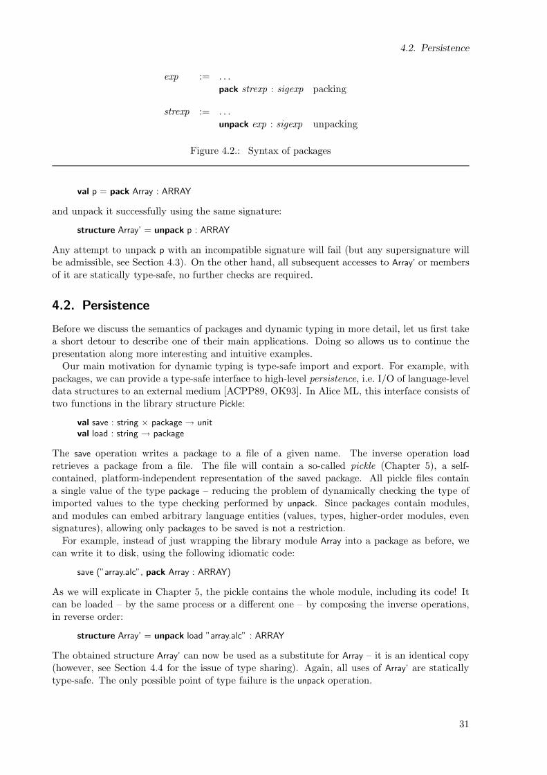
4.2. Persistence
exp := . . .pack strexp : sigexp packing
strexp := . . .unpack exp : sigexp unpacking
Figure 4.2.: Syntax of packages
val p = pack Array : ARRAY
and unpack it successfully using the same signature:
structure Array’ = unpack p : ARRAY
Any attempt to unpack p with an incompatible signature will fail (but any supersignature willbe admissible, see Section 4.3). On the other hand, all subsequent accesses to Array’ or membersof it are statically type-safe, no further checks are required.
4.2. Persistence
Before we discuss the semantics of packages and dynamic typing in more detail, let us first takea short detour to describe one of their main applications. Doing so allows us to continue thepresentation along more interesting and intuitive examples.
Our main motivation for dynamic typing is type-safe import and export. For example, withpackages, we can provide a type-safe interface to high-level persistence, i.e. I/O of language-leveldata structures to an external medium [ACPP89, OK93]. In Alice ML, this interface consists oftwo functions in the library structure Pickle:
val save : string × package → unitval load : string → package
The save operation writes a package to a file of a given name. The inverse operation load
retrieves a package from a file. The file will contain a so-called pickle (Chapter 5), a self-contained, platform-independent representation of the saved package. All pickle files containa single value of the type package – reducing the problem of dynamically checking the type ofimported values to the type checking performed by unpack. Since packages contain modules,and modules can embed arbitrary language entities (values, types, higher-order modules, evensignatures), allowing only packages to be saved is not a restriction.
For example, instead of just wrapping the library module Array into a package as before, wecan write it to disk, using the following idiomatic code:
save (”array.alc”, pack Array : ARRAY)
As we will explicate in Chapter 5, the pickle contains the whole module, including its code! Itcan be loaded – by the same process or a different one – by composing the inverse operations,in reverse order:
structure Array’ = unpack load ”array.alc” : ARRAY
The obtained structure Array’ can now be used as a substitute for Array – it is an identical copy(however, see Section 4.4 for the issue of type sharing). Again, all uses of Array’ are staticallytype-safe. The only possible point of type failure is the unpack operation.
31
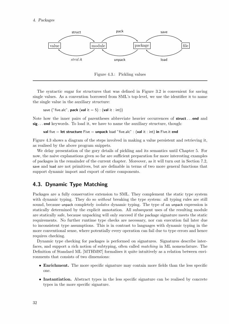
4. Packages
value module package file
struct pack save
loadunpackstrid .it
Figure 4.3.: Pickling values
The syntactic sugar for structures that was defined in Figure 3.2 is convenient for savingsingle values. As a convention borrowed from SML’s top-level, we use the identifier it to namethe single value in the auxiliary structure:
save (”five.alc”, pack (val it = 5) : (val it : int))
Note how the inner pairs of parentheses abbreviate heavier occurrences of struct . . . end andsig . . . end keywords. To load it, we have to name the auxiliary structure, though:
val five = let structure Five = unpack load ”five.alc” : (val it : int) in Five.it end
Figure 4.3 shows a diagram of the steps involved in making a value persistent and retrieving it,as realised by the above program snippets.
We delay presentation of the gory details of pickling and its semantics until Chapter 5. Fornow, the naive explanations given so far are sufficient preparation for more interesting examplesof packages in the remainder of the current chapter. Moreover, as it will turn out in Section 7.2,save and load are not primitives, but are definable in terms of two more general functions thatsupport dynamic import and export of entire components.
4.3. Dynamic Type Matching
Packages are a fully conservative extension to SML. They complement the static type systemwith dynamic typing. They do so without breaking the type system: all typing rules are stillsound, because unpack completely isolates dynamic typing. The type of an unpack expression isstatically determined by the explicit annotation. All subsequent uses of the resulting moduleare statically safe, because unpacking will only succeed if the package signature meets the staticrequirements. No further runtime type checks are necessary, nor can execution fail later dueto inconsistent type assumptions. This is in contrast to languages with dynamic typing in themore conventional sense, where potentially every operation can fail due to type errors and hencerequires checking.
Dynamic type checking for packages is performed on signatures. Signatures describe inter-faces, and support a rich notion of subtyping, often called matching in ML nomenclature. TheDefinition of Standard ML [MTHM97] formalises it quite intuitively as a relation between envi-ronments that consists of two dimensions:
• Enrichment. The more specific signature may contain more fields than the less specificone.
• Instantiation. Abstract types in the less specific signature can be realised by concretetypes in the more specific signature.
32
4.4. Dynamic Type Sharing
Subtyping hence allows a great amount of flexibility with respect to composing modules. Inparticular, it is robust against extension or specialisation of a module interface. That is essentialfor adequately describing program architectures in a modular manner.
Obviously, robustness against future extensions is even more desirable in – potentially ever-changing – dynamic applications. Packages provide it to a wide extent, by having the dynamictype check verify the package signature up to the subtype relation. When a client processretrieves a module from some external location, only minimum assumptions about its signatureneed to be made. The provider of the module is free to replace it with a richer version, as longas the new interface just extends or refines the previous one. All client code will continue towork. In fact, even incompatible changes of the interface will work with clients that did notmake assumptions about that part of the module because they did not access it.
For example, consider a provider offering a package implementing efficient functional dictio-naries over strings:
type α dictval empty : α dictval insert : α dict × string × α → α dictval lookup : α dict × string → α optionval filter : (α → bool) × α dict → α dict
A client retrieves and unpacks the module as follows:
structure Rat = unpack load ”Dict” :sig
type α dictval empty : α dictval insert : α dict × string × α → α dictval lookup : α dict × string → α option
end
Note that the signature does not mention the filter function, since the client does not use it.Consequently, the client will not break if the module one day is changed and extended tosupport the following signature:
type α dictval empty : α dictval insert : α dict × string × α → α dictval lookup : α dict × string → α optionval filter : (string × α → bool) × α dict → α dictval adjoin : α dict × α dict → α dict
Neither the added function adjoin nor the modified type of the filter function will affect the client,the signature still matches the one it assumed.
4.4. Dynamic Type Sharing
In Section 4.2 we claimed that the module Array’ obtained by pickling and unpickling the originallibrary module Array is an identical copy. Although that is true, there is a caveat: the ARRAY
signature contains the abstract type array. The way we unpacked it, the type Array’.array willbe statically incompatible with the original type Array.array. Since there generally is no way todetermine statically what type identities are found in a package, all abstract types in the targetsignature must indeed be considered fully abstract – and hence different from any other – by the(static) type system. The copy can hence only substitute the original as far as type compatibilityis not required.
33
4. Packages
However, type compatibility can be obtained easily – we just need to enforce it in the usualML way, namely by putting type sharing constraints on the target signature:
structure Array’ = unpack Pickle.load ”array.alc” : ARRAY where type array = Array.array
With this formulation, the type Array’.array is statically known to be equal to Array.array. Ofcourse, unpacking will only succeed if the package actually meets this requirement at runtime.
The constraint effectively expresses dynamic type sharing. By restricting the target signaturewe ensure static compatibility, for the price of precluding successful use of non-standard imple-mentations of arrays. Much like for programming with functors, it depends on the applicationhow much sharing is required. Section 4.7 will demonstrate more intricate uses of dynamic typesharing.
4.4.1. Package Signature Refinement
There is a subtlety involved in the previous example: dynamic type sharing works as demon-strated only because the package signature supplied with a pack expression is interpreted trans-parently. That is, writing
val p = pack Array : ARRAY
actually is equivalent to
val p = pack Array : ARRAY where type α array = α Array.array
This behaviour mirrors the semantics of SML’s transparent ascription operator (:), but dy-namically: the actual package signature is obtained by refining the ascribed signature with theconcrete types found in the respective module. Technically, dynamic selfification [HL94], orstrengthening [Ler94], is performed.
As we pointed out in [Ros06], it is worth noting that without the transparent interpretation,the fragment
val p = pack Array : ARRAYstructure Array’ = unpack p
: ARRAY where type α array = α Array.array
would fail with an Unpack exception (as one would expect), but the contorted, yet seeminglyequivalent example
val p = pack Array : ARRAYstructure Aux = unpack p : ARRAYval p’ = pack Aux : ARRAY where type α array = α Aux.arraystructure Array’ = unpack p’
: ARRAY where type α array = α Array.array
would still succeed. Obviously, such pathological behaviour is neither desirable nor useful, thuswe chose the transparent interpretation.
In summary, the transparent interpretation maintains consistency between a package signatureand the contained module. That allows a package to be unpacked with the most specific type ofthe contained module and saves the programmer from cluttering pack expressions with redundantwhere constraints to achieve type propagation.
Note that, due to the presence of abstract signatures (Section 3.3.2), the necessary refinementof the package signature cannot be determined statically in all cases. For example, consider afunctor that corresponds to an η-expansion of the pack operator:
34
4.5. Parametricity
functor Pack (signature S) (X : S) = (val it = pack X : S)
Applying that functor to Array,
val p = let structure P = Pack (signature S = ARRAY) Array in P.it end
should have the same effect as the previous definition of p. Obviously, this requires the signature S
to be dynamically refined inside the functor. Thus, package signatures are generally constructedat runtime.
4.5. Parametricity
The integration of dynamic typing has a severe impact on the semantics of the language: byutilising dynamic type sharing it is possible to dynamically test for type equivalences and have aprogram behave differently depending on the outcome of such a test. Consequently, evaluation isno longer parametric [Rey83, BFSS89, ACC93]. Intuitively, a polymorphically typed expressionis parametric if its evaluation is independent of the concrete type instantiation. A language issaid to be parametric if all polymorphism is parametric.
Parametricity is a valuable property for polymorphic languages, offering important advan-tages:
• Type erasure. Programs can be compiled and executed without maintaining costly typeinformation at runtime.
• Theorems [Wad89]. Polymorphic types state strong invariants about terms, which allowderiving a variety of useful laws.
• Abstraction [Rey83, MP88]. It is possible to achieve encapsulation solely by abstractingor quantifying over types.
Looking closer, it is obvious that evaluation of modules cannot be parametric in the presenceof packages – the behaviour of unpack must depend on dynamic type information. However,for Alice ML the semantics of dynamic types has been crafted such that the core language,where polymorphism is ubiquitous, is not affected. In particular, unlike functors, polymorphicfunctions are still fully parametric: the usual laws still hold, and they can be compiled usingstandard type erasure techniques.
This nicely fits the syntactic setup of ML: on the module level, passing types is always madeexplicit in the syntax. Core polymorphism, on the other hand, is completely implicit. Thus thesyntax provides a clear model to the programmer: only types explicitly supplied in a program, bymeans of named type declarations, can potentially affect its operational behaviour, and inducea cost.
In order to maintain parametricity for core polymorphism we need strict separation betweenimplicit and explicit types. More precisely, it is required that no operation consuming dynamictypes – i.e. unpack and sealing (Section 4.1) – may ever depend on the instantiation of a poly-morphic type variable. Fortunately, this comes for free, thanks to ML’s syntactic treatment oftype variables: both these operations require a signature to be written explicitly. Signature ex-pressions can only refer to other type and signature declarations (possibly nested in structures),and there are only two places in type or signature declarations where type variables can occur:
1. in type declarations and specifications, where type variables on the right side always haveto refer to variables bound on the left side,3
3Actually, that very restriction is missing from the 1997 revision of the SML Definition [MTHM97], but itsabsence has been confirmed as a mistake on part of the Definition, because it leads to unsoundness [Ros01].
35
4. Packages
2. in value specifications, where all type variables occurring in the type are interpreted asuniversally quantified (except for exception specifications, where they are explicitly disal-lowed).
Together, the closedness restriction on type declarations and the implicit local quantification invalue specifications ensure that no dynamic type can depend on a polymorphic type variable,even with local modules (Section 3.2). That is a sufficient condition to maintain parametricityin the extended language Alice ML. For instance,
fun α mypack (x : α) = pack (val it = x) : (val it : α) (* illegal! *)
will not type check, because the local α in the signature is considered locally quantified (andhence different from the one bound at the surrounding declaration), and x does not have theuniversal type ∀α.α. Neither is it possible to type the package by using an auxiliary typedeclaration,
fun α mypack (x : α) =let
type t = α (* illegal! *)in
pack (val it = x) : (val it : t)end
because the local type declaration for t, containing a free occurrence of α, is not allowed by theSML Definition. There is no way to make the package signature refer directly or indirectly tothe polymorphic type variable α, therefore the package signature cannot depend on it.
4.5.1. Working Around Parametricity
Maintaining parametricity in the core language is not without drawback – there is a tensionbetween desirable properties and expressiveness. The fact that ordinary core-level evaluationcannot directly depend on types may appear to be a severe restriction in some dynamic scenarios.The expressive power of dynamic typing remains relatively limited, maybe too limited.
However, that objection can be diluted by the existence of work-arounds that allow emulatingmost of the missing expressiveness:
• Local modules and higher-order functors (Chapter 3) often enable lifting polymorphicfunction definitions to the module level, by turning them into functors. For example, thefunction mypack from above can be reformulated straightforwardly as a functor:
functor MyPack (type t; val x : t) = (val p = pack (val it = x) : (val it : t))
Thanks to local modules, a functor formulation is possible even for local functions. How-ever, this technique potentially requires turning all polymorphic functions up the call chaininto functors, which might quickly become unwieldy. Moreover, the module language is notTuring-complete, so not all desired functions may be expressible (still, it contains SystemFω).
• A more general work-around is to abuse packages as means for communicating types andmodules as first-class values. By wrapping types into packages, they can be passed to corefunctions, which may unpack them locally in order to perform consecutive dynamic typeoperations. Of course, that approach could be deemed somewhat questionable, becauseit essentially means evading the static type system and relying on dynamic typing morethan necessary.
36
4.6. Abstract Types
• If this should prove to be insufficient, adding conventional first-class modules [Rus00] tothe language would be a general solution.
So far, we have only encountered few interesting examples – in the context of what dynamictyping in Alice ML is intended for – which needed to employ any work-around, and the formertwo were adequate enough in those cases.
If the availability of non-parametric core functions should be deemed necessary, the advan-tages of parametricity could still be generally maintained. Instead of abolishing parametricityaltogether, two kinds of type variables could be distinguished, namely conventional ones, whichstay parametric and can be erased, and dynamic ones, that can be used to represent dynamictypes. Parametric variables could be instantiated with types containing dynamic ones, but notvice versa. Something similar has been proposed by Dubois, Rouaix & Weis to support genericfunctions [DRW95]. It is relatively straightforward to extend ML type inference accordingly.
4.6. Abstract Types
An important purpose of a type and module system is erecting and statically verifying abstrac-tion boundaries [Mor73b]. Type abstraction is the respective tool given to the programmer bythe type system. It also is the central feature of the ML module system, where it is supportedthrough sealing (Chapter 3). The ML type system guarantees abstraction safety : values of ab-stract type can only be constructed and deconstructed by the implementation of the abstractionitself. There is no means within the language that allows client code to break an abstraction.
As we saw in the previous section, Alice ML lacks full parametricity. In that situation,type abstraction cannot be guaranteed by means of static scoping of type variables, as in thestandard models of abstract types that are based on existential quantification [MP88, Ros03].The addition of dynamic typing thus raises an important question: Should dynamic typing berequired to respect abstraction? Or can we allow to explicitly overcome abstraction barriers bymeans of dynamic typing?
Alice ML takes a clear stance: type abstraction is a central feature of the ML type system,and no code should be able to sneak across an abstraction barrier. Abstraction safety shall bemaintained at all times. For example, consider an abstract type for generating time stamps:
signature STAMP = (eqtype stamp; val stamp : unit → stamp)structure Stamp :> STAMP =struct
type t = intval state = ref 0fun stamp () = (state := !state+1; !state)
end
The abstraction guarantees that every call to stamp actually delivers a fresh, distinct stamp.Hence it is crucial that the following code cannot be executed successfully:
val p = pack (val x = 13) : (val x : int)structure Fake = unpack p : (val x : Stamp.t)
If the unpack operation succeeded, we would have forged a bogus stamp value – the stamp proce-dure would no longer be guaranteed to deliver distinct values. Hence we need unpack to fail in thisexample. Apparently, this means that Stamp.t must be a type different from int – dynamically!
Alice ML achieves the desired semantics by employing dynamic generativity. That is, everyabstract type is represented by a dynamic type name, and this name is generated at runtime,when the respective declaration is evaluated. In particular, sealing, i.e. evaluating a structureexpression of the form
37
4. Packages
strexp :> sigexp
generates a new name for every type specified abstractly in the signature sigexp. This happenseach time the expression is evaluated, hence the functor
functor MkStamp () :> STAMP =struct
type t = intval state = ref 0fun stamp () = (state := !state+1; !state)
end
generates multiple distinct stamp types when applied multiple times – exactly as suggested bythe static semantics of SML.
Dynamic type names are globally unique. In general, this is necessary to avoid forging ofabstract values by other processes. Pickling (Section 4.2) allows arbitrary values to be madepersistent or be exchanged between different processes, and this includes values of abstract type.In order to maintain abstraction safety, the type names generated in one process must hence bedifferent from any type name generated in any other process, at any time.
4.6.1. Internal and External View of Abstraction
Though the dynamic semantics of sealing and type generativity are relatively straightforward,they can have subtle effects. In particular, sealing is performed after evaluating the sealed mod-ule itself. Consequently, the module’s internals know nothing about the type names generated.As statically, a dynamic type abstracted via sealing is fully transparent inside the abstraction.Dynamic types crossing abstraction boundaries may hence not satisfy equivalences one mightnaively expect. For example, after evaluating
structure M :> (type t; val f : t → string) =struct
type t = intfun f x = Int.toString xval = Pickle.save (”m.alc”, pack (val it = 37) : (val it : t))
end
the type M.t, being opaque, is different from the type occurring in the signature of the packagewritten to the file, which is just int. Hence
structure It = unpack Pickle.load ”m.alc” : (val it : M.t)
will fail. On the other hand,
structure It = unpack Pickle.load ”m.alc” : (val it : int)
actually succeeds! Probably not what is desired. The problem is that there are two incompatibleviews of an abstract type, the internal and the external one. The type system ensures thatthe views are properly switched whenever a value of the abstract type crosses the abstractionboundary. If we, like in the example above, sidestep the static type system by passing such avalue dynamically typed, then the type system cannot know about that. Abstractions need tobe implemented such that this does not happen.
Fortunately, occasions where the abstraction has to construct a dynamic value of abstract typeinternally – like above – are rare. The desired effect can always be achieved by a two-stagedconstruction:
38
4.7. Typeful Dynamic Programming
structure M : (type t; val f : t → string) =struct
structure Abs :> (type t; val it : t; val f : t → string) =struct
type t = intfun f x = Int.toString x
end
open Absval = Pickle.save (”m.alc”, pack (val it = Abs.it) : (val it : Abs.t))
end
In general, the main implementation of an abstraction would go into a sealed, inner auxiliarystructure like Abs. Only operations requiring access to the abstract type name are definedoutside. Note that the outer signature ascription is transparent, in order not to generate asecond level of abstraction that would defeat the whole purpose of the construction.
4.7. Typeful Dynamic Programming
No abstraction can be breached by means of dynamic typing. But is that behaviour useful? Canwe really work with rock-solid abstract types in the context of open programming? For example,when a process pickles a value of abstract type, and the type was created by the process, how canthe value ever be unpacked after that process has terminated? Due to the generative semanticsof sealing, even a subsequent process running the same program will not be able to unpack it.
The answer is quite simple: one has to export and share the abstraction as well. Recall thatall import/export is based on packages, and packages contain modules. Hence it is perfectlyvalid to pickle the module implementing an abstraction. In fact, dynamic type sharing canbe employed for typeful programming [Car91] with dynamic types, when packages themselvescontain the implementation of abstract types.
Consider a strategy game. It allows initiating a new campaign, and during a campaign arbi-trary snapshots (saved games) can be stored that allow reverting to that point of the campaignlater on. When the program is exited, the current campaign is pickled and can be continuednext time the game is started. At any point, a stored snapshot can be loaded.
Different campaigns may use different configurations (e.g. map sizes). A snapshot only isvalid in conjunction with the campaign that it belongs to. To prevent mixing up snapshots ofincompatible campaigns, a snapshot can be modelled as an abstract type that is created alongwith a particular campaign. More precisely, a campaign is a structure with the signature
signature CAMPAIGN =sig
type worldval getWorld : unit → worldval setWorld : world → unit...
end
where the abstract type world encapsulates the state of the campaign. A new campaign mightbe created by means of a functor:
functor MkCampaign (Config : CONFIG) :> CAMPAIGN = ...structure Campaign = MkCampaign MyConfig
A fresh world type is generated along with an initial world state. A snapshot of a campaign cannow be created by retrieving its current world and pickling it to a file:
39
4. Packages
Pickle.save (”snapshot”, pack (val world = Campaign.getWorld ()) : (val world : Campaign.world))
As long as the application has not terminated, it is easy to reload previous snapshots of therunning campaign:
structure W = unpack Pickle.load ”snapshot” : (val world : Campaign.world)Campaign.setWorld W.world
When the application exits, it pickles the campaign itself:
Pickle.save (”campaign”, pack Campaign : CAMPAIGN)
When the game is run the next time the user can choose to continue an existing campaign, ata given snapshot. This is implemented by unpickling the previous campaign instead of creatinga new one, along with the selected snapshot:
structure Campaign = unpack load ”campaign” : CAMPAIGNstructure W = unpack Pickle.load ”snapshot” : (val world : Campaign.world)Campaign.setWorld W.world
Unpacking the snapshot will only succeed if it actually belongs to the given campaign. What wesee in the example is an interesting instance of dynamic type sharing (Section 4.4): the signatureused to unpack one module refers to a type dynamically obtained from another package. Thegenerative semantics of sealing (Section 4.6) makes it possible to detect type sharing dynamically,while still not being able to discover the underlying implementation types.
In simple examples like the above, type sharing is straightforward to express, because theascribed signature can easily be given inline. In order to deal with more complex examples,SML’s module system already provides features for expressing more involved type sharing: typeconstraints on signatures, i.e. type specialisation using where as well as sharing specifications,both useful in the static type system, will come in handy for dynamic typing as well.
Assume that a campaign snapshot should not only contain the state of the game world, butalso some meta information like when the snapshot was created, on what system, etc. In thatcase, it is more convenient to define a signature:
signature SNAPSHOT =sig
type worldval world : worldval date : dateval system : string...
end
The world type has to be abstract in the signature, because it will differ between uses. In orderto concretise it when we ascribe the respective unpack operation, we simply put a respectiveconstraint on the signature:
structure Campaign = unpack Pickle.load ”campaign” : CAMPAIGNstructure World =
unpack Pickle.load ”snapshot” : SNAPSHOT where type world = Campaign.world
In general, the same language mechanisms are applicable for expressing dynamic sharing withpackages as for expressing static sharing between functor parameters. No additional structurein the type language is necessary. The introduction of dynamic typing stays economic from asemantic point of view and, to a large extent, enables the programmer to reuse her knowledgeabout expressing type relations with modules.
40
4.8. Related Work
4.8. Related Work
In previous work we have presented the basic design of packages in Alice ML [RLT+06], andwe have formalised packages and pickling as part of a calculus of higher-order modules [Ros06]that we proved sound. The latter work gives a relatively direct type-theoretic account for thesemantics of packages. We also have integrated a formalisation of packages directly into theformal language specification of Standard ML [Ros05].
The concept of dynamics has long been folklore. Dynamics were already proposed for the verypurpose of open programming in an unpublished article by Mycroft [Myc83], and later madeprecise by Abadi, Cardelli, Pierce & Plotkin [ACPP91, ACPR95]. Their proposal involved acomplex typecase construct for projection, in order to dispatch on the type of the dynamic. Ourunpack operator is less expressive, although type dispatch can be simulated to a certain extendby a sequence of unpack operations with different signatures. On the other hand, unpack supportssubtyping, hence making the use of packages more flexible and robust against changes. In ourexperience, this dimension actually is much more important for the applications dynamics areintended for.
Some typed languages offer slightly different variations of dynamic typing. Alanko [Ala04]gives an overview of the use of dynamic typing and reflection in typed languages.
The syntax for package injection and projection has been borrowed from Russo’s work on first-class modules [Rus00, Rus98], and indeed there is a close relation. The fundamental differencebetween packages and first-class modules is that the latter are statically typed (i.e. the typeof a module value describes its full signature), while packages are dynamically typed (the typepackage is abstract).
A package can be understood as a first-class module wrapped into a conventional dynamic.However, coupling both mechanisms enables unpack to exploit subtype polymorphism, which isnot possible otherwise, due to the lack of subtyping in the ML core language. For example,assume two signatures S ≤ S′. Given a package with signature S we can unpack it undersignature S′, without actually knowing S. With dynamics and first-class modules however,given a dynamic carrying a first-class module of signature S, i.e. a value of type 〈S〉, we firstwould have to unwrap the dynamic under type 〈S〉 – since there is no subtyping in the corelanguage, we would have to know S exactly at this point. We could only go to S′ after havingprojected the module. Clearly, this would severely weaken modularity and robustness.
4.9. Summary
• We introduce packages as a novel variant of dynamics; they carry a module along with itsdynamic signature.
• Accessing a package requires a dynamic type-check against a static target signature.
• The type-check employs structural subtyping to make clients robust against interfacechanges.
• Based on packages, Alice ML provides type-safe persistence.
• Dynamic type sharing can be expressed with idioms known from ML modules, and enablestypeful dynamic programming.
• Unlike with previous work on dynamics, dynamic typing is confined to the module lan-guage, the core language is still parametric.
• Abstraction safety is maintained within the language – type abstraction dynamically gen-erates fresh, globally unique type names.
41

4. Packages
42
5. Pickling
The most important characteristic of an open program is the need to communicate with theoutside world. More precisely, an open program has to exchange information with its environ-ment, other programs, or other instances of the same program. In a high-level language, wewant to be able to represent such information as language-level values wherever possible. Thatis, the language should enable us to import and export potentially arbitrary language-level datastructures. In a higher-order language with first-class functions, that naturally includes func-tions, and hence code – opening up a whole range of applications for exchanging functionalityand behaviour. Furthermore, in a language with strong emphasis on types and modules forstructuring data and functionality, we want to be able to exchange entire program fragments inthe form of modules.
The task of exporting a value from a process is often known as serialisation or marshalling.For reasons discussed in the next section, we prefer the somewhat less common term pick-ling [BJW87].
Unlike the features discussed in the previous chapters, pickling is not a language constructper se, but rather a generic mechanism underlying a number of other language constructs.Nevertheless, its central role and recurring semantic implications justify treatment in a separatechapter.
Pickling or related mechanisms have been employed in many previous languages to sup-port persistence and inter-process communication, e.g. CLU [HL82], Modula-3 [BNOW95], orJava [RWWB96]. The Mozart System for Oz was the first to systematically and uniformlybase its compilation and distribution model on pickles, in particular by supporting pickling ofcode [DKSS98]. Alice ML adopts the Oz approach and puts it into a typed context.
5.1. Pickles
In order to export a value from a process, it must be transformed into an external representation.To support open programming in a most general and safe way, we require several properties ofsuch a representation:
• Transparency. The composition of pickling and unpickling a value should yield a copythat is observationally equivalent to the original value.
• Universality. The representation should support all possible types of values found in thelanguage. In particular, it should readily support higher-order and user-defined types, aswell as cyclic structures. The only exceptions are primitive types whose meaning is boundto the current process, so-called resources (e.g. file handles, thread names, etc.).
• Closedness. An external representation should always be self-contained. That is, itshould contain the transitive closure of all values reachable by the one meant to be ex-ported. For functions, it has to include their code.
• Portability. The representation should be independent from and portable between dif-ferent computer architectures, operating systems, and implementations of the language.
43
5. Pickling
• Verifiability. It should be possible to test the integrity of an external representation, i.e.the format must be self-describing enough to support checking that a given instance reallyrepresents a well-formed value of the language.
• Security. An external value should not be allowed to contain references to critical re-sources that might enable contained functions to silently perform unapproved, security-relevant actions when applied on an importing site.
• Efficiency. The space required for the representation of a value should be at most linearin the size it takes in memory. That particularly implies that sharing between values in aclosure must be maintained.
We call an external representation meeting these requirements a pickle. This terminology em-phasises the fact that it is really a self-contained representation, which is not the case for mostexisting serialisation or marshalling mechanisms, especially with respect to code.
Obviously, the requirement for universality demands pickling to be made available as a genericmechanism. A library or user-defined infrastructure, like often found in other languages, is notenough, because it could not deal with functions, abstract types, or modules, etc. In Alice ML,pickling, and its inverse, unpickling, thus need to be built-in services of the runtime system.Pickling takes a value and produces a copy that can be transferred to other processes. On amore technical level, pickling transforms the internal graph-like representation of an object inmemory into a linear, platform-independent external representation [TKS06, Tac03]. From apickle an equivalent copy of the original object can be reconstructed. A pickle includes thetransitive closure of the respective object, i.e. the reachable subgraph. This graph can be cyclic.
For a rich language like ML, designing and specifying a pickle format that meets all of theabove requirements is a complex endeavour. In particular, it implies giving a full specificationof the external code format of the language. Furthermore, it involves specifying a low-leveltype system to support verification of code and data. This in turn has potential impact on theimplementation of a runtime system for the language, because it must be able to produce thistype information upon pickling.
Clearly, such questions are beyond the scope of this thesis. Here, we are only concerned withthe design and semantics of the mere language, not its implementation. We hence stay in orbitof these issues and take the desired properties for granted, as far as they are transparent in thesemantics.1 We refer the interested reader to the works of Kornstaedt and Tack [TKS06, Kor06,Tac03] for an in-depth discussion of the design and implementation of a pickling mechanism.
Another aspect we generally remain naive about in this thesis is security. We consider securityissues only as far as not making the language semantics violate obvious security concerns inirreparable manners, and by providing some hooks to implement more elaborate strategies.
5.2. Type checking and verification
In Alice ML, almost arbitrary language-level data structures can be pickled. How do we achievetype-safety if we allow values of arbitrary type to be retrieved from files at runtime? How cana load operation be typed, when it is impossible for the compiler to know what files will beaccessed dynamically, and what types of values they contain?
Obviously, loading pickles generally requires dynamic checks to establish type-safety. We candistinguish two kinds of check:
1The current version of the Alice System does not yet meet all of the requirements. In particular, the pickleformat does only support a rudimentary amount of verification, and no attempt has been made to actuallymake the system a secure platform.
44
5.2. Type checking and verification
• Verification. Checks internal consistence of a pickle, i.e. whether it represents a well-formed value (of a fixed type).
• Dynamic Typing. Checks external consistence, i.e. compares the type of the pickle withthe one expected by the consuming code.
Both these checks are orthogonal: if the producer of a pickle is trusted, verification may beomitted; if the type of the value represented by the pickle is known statically, dynamic typing isnot needed. In the latter case, the pickle need not include a description of its own type, becauseit can be determined from context. All combinations are possible – consider the followingscenarios:
• Persistence: the content type of a file cannot be known statically, hence dynamic typingis required; however, if the environment is trusted, we may omit verification of the file.
• Typed communication channel: the channel type determines the type of values receivedover the channel, hence it need not be transmitted nor checked for each value (it is checkedonce when the connection is established). However, if the sender is untrusted, the individ-ual values must still be verified to be well-formed with respect to that type.
Moreover, although both checks can be understood as a form of dynamic type checking, theirnature is quite different: verification has to look at the structure of a pickle, while dynamic typingcan be realised simply by comparing a type description that is part of the pickle (and mightitself require verification). Both checks operate on different levels of abstraction. For example,verification must be able to see the representation of abstract types, while dynamic typingshould not (Section 4.6). Verification might involve more (and lower-level) type informationthan visible in the type system of the language, because it has to encompass internal invariantsof the low-level representation, especially of code.2
Thanks to packages, we can separate concerns: we uncouple dynamic typing from (un)picklinginstead of building it into the pickling mechanism. We rely on packages as an independentmechanism, while unpickling itself only performs verification (if necessary).
Section 4.2 briefly introduced the primitives for persistence provided in Alice ML:
val save : string × package → unitval load : string → package
All pickle files thus created contain values of one and the same type, package, thus supportingdynamic typing. The idiomatic usage of the primitives then is as follows:
save (”file.alc”, pack Module : SIG)structure Module’ = unpack load ”file.alc” : SIG’
The code clearly separates the two kinds of checks discussed above:
• The load operation has to perform verification, i.e. checks that the file contains a well-formed pickle, representing a package. Failure at this point is considered I/O failure.3
• The unpack operator has to check that the package signature matches the static assump-tions, i.e. the target signature. Failure at this point is a dynamic type error.
2Alternatively, verification can also be substituted by authentication. In that approach, pickles are signedusing cryptographic methods, and only pickles stemming from trusted authorities are accepted as well-formed.Obviously, this is less flexible, but might be sufficient for certain scenarios. We will not explore that possibilityhere.
3As mentioned, this check is not properly implemented in the current version of Alice.
45
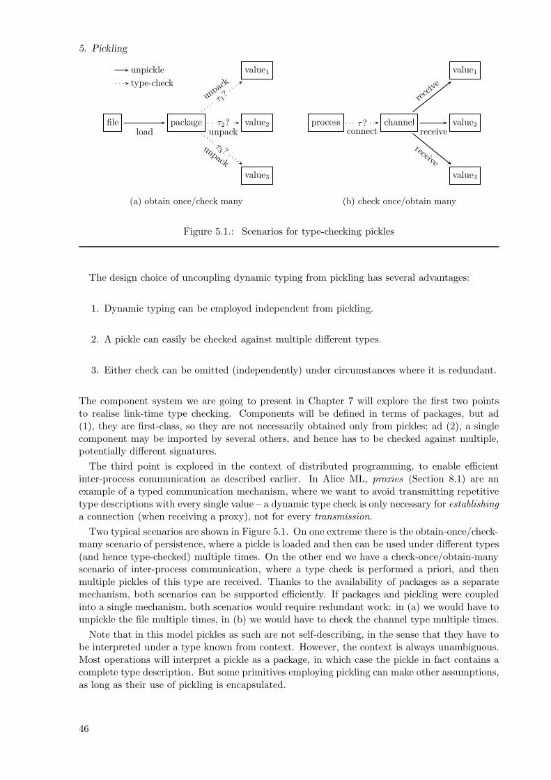
5. Pickling
(a) obtain once/check many
file package
value1
value2
value3
load
unpa
ck
τ1?
unpackτ2?
unpack
τ3 ?
unpickle
type-check
(b) check once/obtain many
process channel
value1
value2
value3
connectτ?
rece
ive
receive
receive
Figure 5.1.: Scenarios for type-checking pickles
The design choice of uncoupling dynamic typing from pickling has several advantages:
1. Dynamic typing can be employed independent from pickling.
2. A pickle can easily be checked against multiple different types.
3. Either check can be omitted (independently) under circumstances where it is redundant.
The component system we are going to present in Chapter 7 will explore the first two pointsto realise link-time type checking. Components will be defined in terms of packages, but ad(1), they are first-class, so they are not necessarily obtained only from pickles; ad (2), a singlecomponent may be imported by several others, and hence has to be checked against multiple,potentially different signatures.
The third point is explored in the context of distributed programming, to enable efficientinter-process communication as described earlier. In Alice ML, proxies (Section 8.1) are anexample of a typed communication mechanism, where we want to avoid transmitting repetitivetype descriptions with every single value – a dynamic type check is only necessary for establishinga connection (when receiving a proxy), not for every transmission.
Two typical scenarios are shown in Figure 5.1. On one extreme there is the obtain-once/check-many scenario of persistence, where a pickle is loaded and then can be used under different types(and hence type-checked) multiple times. On the other end we have a check-once/obtain-manyscenario of inter-process communication, where a type check is performed a priori, and thenmultiple pickles of this type are received. Thanks to the availability of packages as a separatemechanism, both scenarios can be supported efficiently. If packages and pickling were coupledinto a single mechanism, both scenarios would require redundant work: in (a) we would have tounpickle the file multiple times, in (b) we would have to check the channel type multiple times.
Note that in this model pickles as such are not self-describing, in the sense that they have tobe interpreted under a type known from context. However, the context is always unambiguous.Most operations will interpret a pickle as a package, in which case the pickle in fact contains acomplete type description. But some primitives employing pickling can make other assumptions,as long as their use of pickling is encapsulated.
46
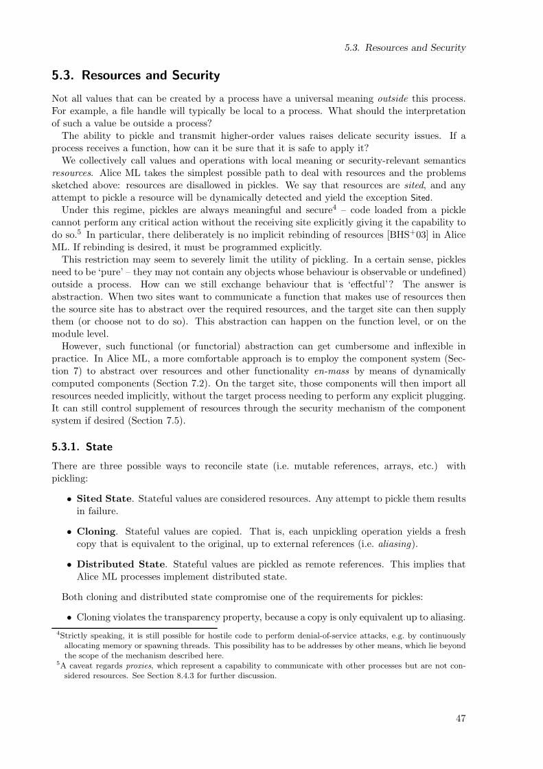
5.3. Resources and Security
5.3. Resources and Security
Not all values that can be created by a process have a universal meaning outside this process.For example, a file handle will typically be local to a process. What should the interpretationof such a value be outside a process?
The ability to pickle and transmit higher-order values raises delicate security issues. If aprocess receives a function, how can it be sure that it is safe to apply it?
We collectively call values and operations with local meaning or security-relevant semanticsresources. Alice ML takes the simplest possible path to deal with resources and the problemssketched above: resources are disallowed in pickles. We say that resources are sited, and anyattempt to pickle a resource will be dynamically detected and yield the exception Sited.
Under this regime, pickles are always meaningful and secure4 – code loaded from a picklecannot perform any critical action without the receiving site explicitly giving it the capability todo so.5 In particular, there deliberately is no implicit rebinding of resources [BHS+03] in AliceML. If rebinding is desired, it must be programmed explicitly.
This restriction may seem to severely limit the utility of pickling. In a certain sense, picklesneed to be ‘pure’ – they may not contain any objects whose behaviour is observable or undefined)outside a process. How can we still exchange behaviour that is ‘effectful’? The answer isabstraction. When two sites want to communicate a function that makes use of resources thenthe source site has to abstract over the required resources, and the target site can then supplythem (or choose not to do so). This abstraction can happen on the function level, or on themodule level.
However, such functional (or functorial) abstraction can get cumbersome and inflexible inpractice. In Alice ML, a more comfortable approach is to employ the component system (Sec-tion 7) to abstract over resources and other functionality en-mass by means of dynamicallycomputed components (Section 7.2). On the target site, those components will then import allresources needed implicitly, without the target process needing to perform any explicit plugging.It can still control supplement of resources through the security mechanism of the componentsystem if desired (Section 7.5).
5.3.1. State
There are three possible ways to reconcile state (i.e. mutable references, arrays, etc.) withpickling:
• Sited State. Stateful values are considered resources. Any attempt to pickle them resultsin failure.
• Cloning. Stateful values are copied. That is, each unpickling operation yields a freshcopy that is equivalent to the original, up to external references (i.e. aliasing).
• Distributed State. Stateful values are pickled as remote references. This implies thatAlice ML processes implement distributed state.
Both cloning and distributed state compromise one of the requirements for pickles:
• Cloning violates the transparency property, because a copy is only equivalent up to aliasing.
4Strictly speaking, it is still possible for hostile code to perform denial-of-service attacks, e.g. by continuouslyallocating memory or spawning threads. This possibility has to be addresses by other means, which lie beyondthe scope of the mechanism described here.
5A caveat regards proxies, which represent a capability to communicate with other processes but are not con-sidered resources. See Section 8.4.3 for further discussion.
47
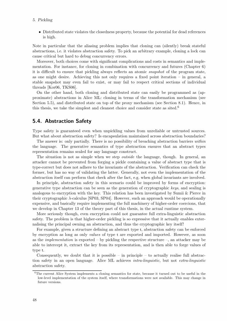
5. Pickling
• Distributed state violates the closedness property, because the potential for dead referencesis high.
Note in particular that the aliasing problem implies that cloning can (silently) break statefulabstractions, i.e. it violates abstraction safety. To pick an arbitrary example, cloning a lock cancause critical but hard to debug concurrency errors.
Moreover, both choices come with significant complications and costs in semantics and imple-mentation. For instance, for cloning in combination with concurrency and futures (Chapter 6)it is difficult to ensure that pickling always reflects an atomic snapshot of the program state,as one might desire. Achieving this not only requires a fixed point iteration – in general, astable snapshot may even fail to exist, or may fail to respect critical sections of individualthreads [Kor06, TKS06].
On the other hand, both cloning and distributed state can easily be programmed as (ap-proximate) abstractions in Alice ML: cloning in terms of the transformation mechanism (seeSection 5.5), and distributed state on top of the proxy mechanism (see Section 8.1). Hence, inthis thesis, we take the simplest and cleanest choice and consider state as sited.6
5.4. Abstraction Safety
Type safety is guaranteed even when unpickling values from unreliable or untrusted sources.But what about abstraction safety? Is encapsulation maintained across abstraction boundaries?
The answer is: only partially. There is no possibility of breaching abstraction barriers withinthe language. The generative semantics of type abstraction ensures that an abstract typesrepresentation remains sealed for any language construct.
The situation is not as simple when we step outside the language, though. In general, anattacker cannot be prevented from forging a pickle containing a value of abstract type that istype-correct but does not adhere to the invariants of the abstraction. Verification can check theformer, but has no way of validating the latter. Generally, not even the implementation of theabstraction itself can perform that check after the fact, e.g. when global invariants are involved.
In principle, abstraction safety in this scenario could be improved by forms of encryption:generative type abstraction can be seen as the generation of cryptographic keys, and sealing isanalogous to encryption with the key. This relation has been investigated by Sumii & Pierce intheir cryptographic λ-calculus [SP03, SP04]. However, such an approach would be operationallyexpensive, and basically require implementing the full machinery of higher-order coercions, thatwe develop in Chapter 13 of the theory part of this thesis, in the actual runtime system.
More seriously though, even encryption could not guarantee full extra-linguistic abstractionsafety. The problem is that higher-order pickling is so expressive that it actually enables exter-nalising the principal owning an abstraction, and thus the cryptographic key itself!
For example, given a structure defining an abstract type t, abstraction safety can be enforcedby encryption as long as only values of type t are exported and imported. However, as soonas the implementation is exported – by pickling the respective structure –, an attacker may beable to intercept it, extract the key from its representation, and is then able to forge values oftype t.
Consequently, we doubt that it is possible – in principle – to actually realise full abstrac-tion safety in an open language. Alice ML achieves intra-linguistic, but not extra-linguisticabstraction safety.
6The current Alice System implements a cloning semantics for state, because it turned out to be useful in thelow-level implementation of the system itself, where transformations were not available. This may change infuture versions.
48
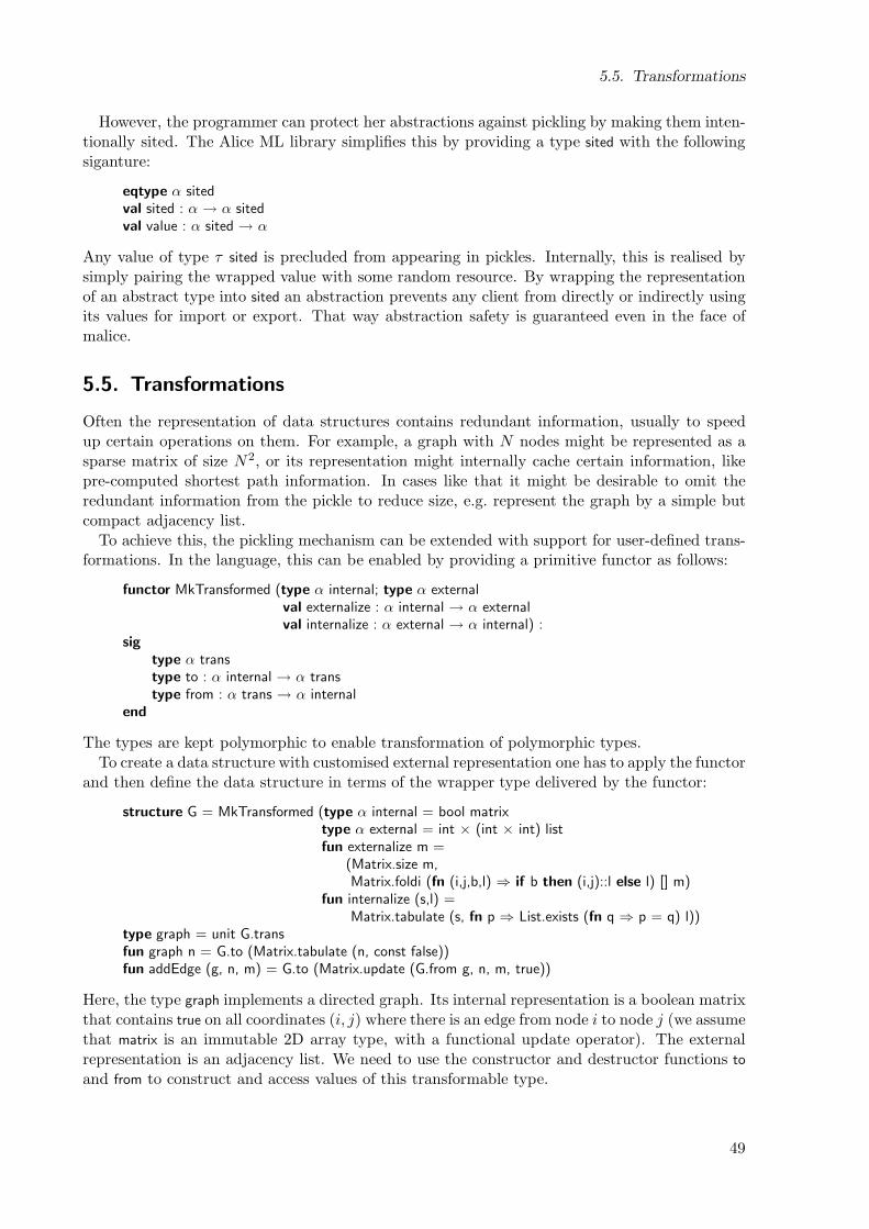
5.5. Transformations
However, the programmer can protect her abstractions against pickling by making them inten-tionally sited. The Alice ML library simplifies this by providing a type sited with the followingsiganture:
eqtype α sitedval sited : α → α sitedval value : α sited → α
Any value of type τ sited is precluded from appearing in pickles. Internally, this is realised bysimply pairing the wrapped value with some random resource. By wrapping the representationof an abstract type into sited an abstraction prevents any client from directly or indirectly usingits values for import or export. That way abstraction safety is guaranteed even in the face ofmalice.
5.5. Transformations
Often the representation of data structures contains redundant information, usually to speedup certain operations on them. For example, a graph with N nodes might be represented as asparse matrix of size N2, or its representation might internally cache certain information, likepre-computed shortest path information. In cases like that it might be desirable to omit theredundant information from the pickle to reduce size, e.g. represent the graph by a simple butcompact adjacency list.
To achieve this, the pickling mechanism can be extended with support for user-defined trans-formations. In the language, this can be enabled by providing a primitive functor as follows:
functor MkTransformed (type α internal; type α externalval externalize : α internal → α externalval internalize : α external → α internal) :
sig
type α transtype to : α internal → α transtype from : α trans → α internal
end
The types are kept polymorphic to enable transformation of polymorphic types.To create a data structure with customised external representation one has to apply the functor
and then define the data structure in terms of the wrapper type delivered by the functor:
structure G = MkTransformed (type α internal = bool matrixtype α external = int × (int × int) listfun externalize m =
(Matrix.size m,Matrix.foldi (fn (i,j,b,l) ⇒ if b then (i,j)::l else l) [] m)
fun internalize (s,l) =Matrix.tabulate (s, fn p ⇒ List.exists (fn q ⇒ p = q) l))
type graph = unit G.transfun graph n = G.to (Matrix.tabulate (n, const false))fun addEdge (g, n, m) = G.to (Matrix.update (G.from g, n, m, true))
Here, the type graph implements a directed graph. Its internal representation is a boolean matrixthat contains true on all coordinates (i, j) where there is an edge from node i to node j (we assumethat matrix is an immutable 2D array type, with a functional update operator). The externalrepresentation is an adjacency list. We need to use the constructor and destructor functions to
and from to construct and access values of this transformable type.
49
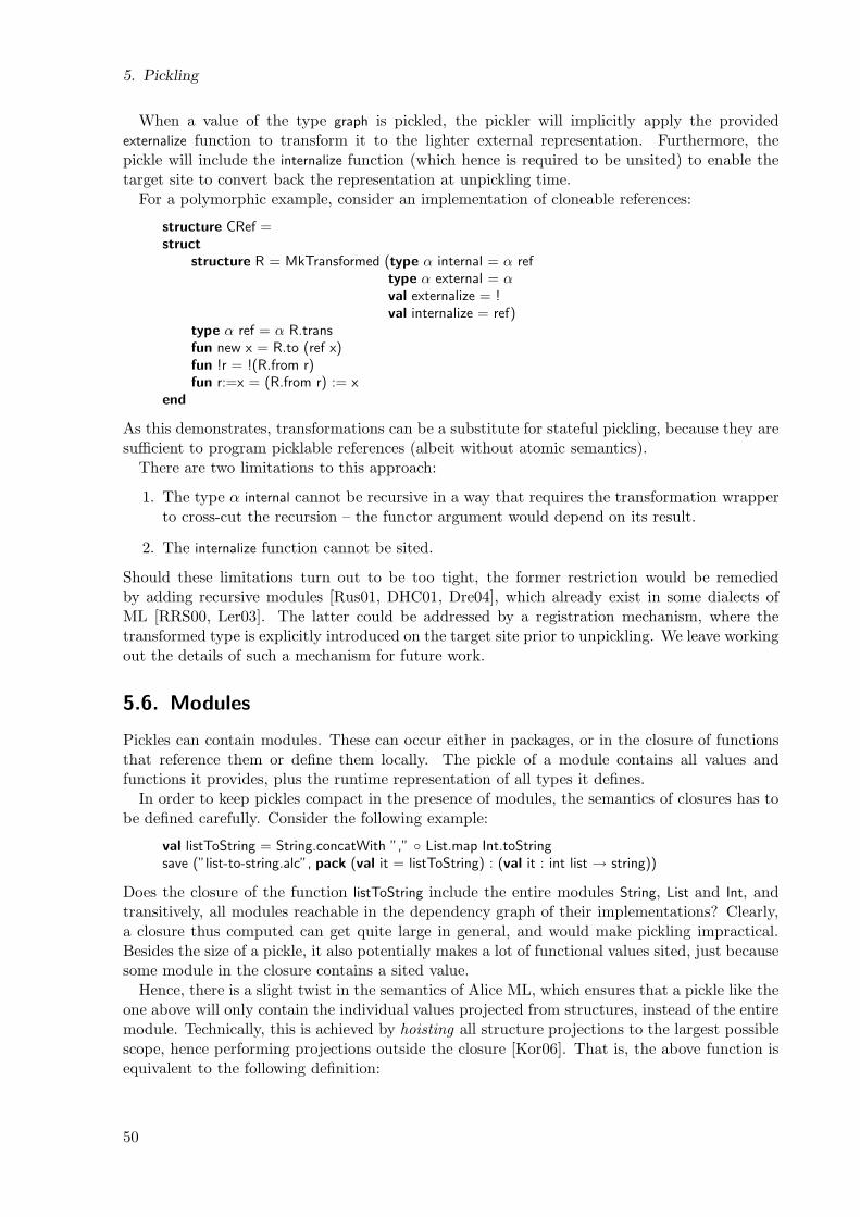
5. Pickling
When a value of the type graph is pickled, the pickler will implicitly apply the providedexternalize function to transform it to the lighter external representation. Furthermore, thepickle will include the internalize function (which hence is required to be unsited) to enable thetarget site to convert back the representation at unpickling time.
For a polymorphic example, consider an implementation of cloneable references:
structure CRef =struct
structure R = MkTransformed (type α internal = α reftype α external = αval externalize = !val internalize = ref)
type α ref = α R.transfun new x = R.to (ref x)fun !r = !(R.from r)fun r:=x = (R.from r) := x
end
As this demonstrates, transformations can be a substitute for stateful pickling, because they aresufficient to program picklable references (albeit without atomic semantics).
There are two limitations to this approach:
1. The type α internal cannot be recursive in a way that requires the transformation wrapperto cross-cut the recursion – the functor argument would depend on its result.
2. The internalize function cannot be sited.
Should these limitations turn out to be too tight, the former restriction would be remediedby adding recursive modules [Rus01, DHC01, Dre04], which already exist in some dialects ofML [RRS00, Ler03]. The latter could be addressed by a registration mechanism, where thetransformed type is explicitly introduced on the target site prior to unpickling. We leave workingout the details of such a mechanism for future work.
5.6. Modules
Pickles can contain modules. These can occur either in packages, or in the closure of functionsthat reference them or define them locally. The pickle of a module contains all values andfunctions it provides, plus the runtime representation of all types it defines.
In order to keep pickles compact in the presence of modules, the semantics of closures has tobe defined carefully. Consider the following example:
val listToString = String.concatWith ”,” List.map Int.toStringsave (”list-to-string.alc”, pack (val it = listToString) : (val it : int list → string))
Does the closure of the function listToString include the entire modules String, List and Int, andtransitively, all modules reachable in the dependency graph of their implementations? Clearly,a closure thus computed can get quite large in general, and would make pickling impractical.Besides the size of a pickle, it also potentially makes a lot of functional values sited, just becausesome module in the closure contains a sited value.
Hence, there is a slight twist in the semantics of Alice ML, which ensures that a pickle like theone above will only contain the individual values projected from structures, instead of the entiremodule. Technically, this is achieved by hoisting all structure projections to the largest possiblescope, hence performing projections outside the closure [Kor06]. That is, the above function isequivalent to the following definition:
50
5.7. Related Work
val Int toString = Int.toStringval String concatWith = String.concatWithval List map = List.mapval listToString = String concatWith ”,” List map Int toString
In order to give a sense for the relevance of this transformation, consider the pickle createdabove. Thanks to the hoisting semantics, it will produce a file of 1181 bytes in the current versionof the Alice System. This pickle contains the code of 8 functions appearing in the transitiveclosure. In a naive semantics, the pickle would contain 9 modules with a total of 210 functionsinstead! Pickling this set of modules takes 18966 bytes with the current library, a more than16-fold increase. Keep in mind that this is a very simple example, only referencing the mostprimitive library modules – for more high-level modules the ratio is likely to get significantlyworse.
It is worth noting that this optimisation crucially relies on the fact that ML is a module-centric language and not an object-oriented one. With modules, a value is free-standing, anddoes not carry any functionality of its own (unless it is of higher-order type). In contrast, in anobject-oriented model every value carries all its methods – either directly, or indirectly throughits class, which will always be part of an object’s closure. No comparable transformation can beapplied, because all methods remain reachable through the original object.
5.7. Related Work
The term pickling was originally coined in the context of databases and operating systems, byBirrell, Jones & Wobber [BJW87]. However, the first programming language that was equippedwith a comparable mechanism already was CLU [HL82], which had a particular focus on typeabstraction, and required the programmer to provide transformation functions to pickle valuesof abstract type. CLU later inspired a similar mechanism for the object-oriented languages Mod-ula 3 [BNOW95] and Java [RWWB96]. Neither of these languages meets all of the requirementsstated in Section 5.1. In particular, they remain limited with respect to universality, closedness,and portability. Only Java ensures the latter and performs verification on class files.
Oz [Smo95, DKSS98, VH04] and the Mozart Programming System directly inspired the pick-ling mechanism found in Alice ML. Like Alice ML, pickling in Oz meets all of the listed require-ments except Verifiability. Since Oz is a dynamically checked language, dynamic typing is notemployed.
Acute [SLW+05] is an ML-based language for distributed programming that is closest to AliceML and also provides a generic pickling mechanism. Unlike in Alice ML, pickling is not separatedfrom dynamic typing (Section 5.2). Also, Acute is not intended to “protect against fraud”,so there is no concept of security: pickles are type-checked but not verified,7 and unpicklingperforms uncontrolled implicit rebinding of resources.
Several other functional languages also provide pickling functionality, for instance SML ofNew Jersey [Luc00] and Objective Caml [Ler03]. In most of them pickling is not even a type-safe operation. The only notable exception is Clean, which features high-level I/O based ondynamics [Pil96].
Kornstaedt [Kor06] discusses the design space of many aspects of pickling in detail, and alsoprovides a more in-depth comparison of the mechanisms available in the forementioned lan-guages. The low-level semantics and implementation of pickling in the Alice System is describedby Tack & Kornstaedt [TKS06, Tac03]. They also describe a generic minimisation mechanism
7As mentioned, Alice ML does not implement this yet either.
51
5. Pickling
(implemented in the Alice System) that reduces the size of pickles by applying automaton min-imization algorithms to the data graph.
We have given a high-level formal semantics of pickling in Alice ML in previous work [Ros06].It closely mirrors the formal development in Chapter 12 of this thesis, but was in the frameworkof a module calculus modelling ML modules. Some of the aspects regarding the role of picklingin Alice ML we present here are also discussed in that and other earlier work [RLT+06].
Kennedy implements a limited form of pickling in form of a combinator library written inML [Ken04]. This is attractive for more lightweight applications like simple data persistence,but as already mentioned, a library approach fails to meet most of the requirements imposedby an open programming scenario (Section 5.1): although surprsingly flexible, Kennedy’s com-binators are neither universal (especially, they cannot deal with function values), nor can theyguarantee properties like transparency, closedness, portability, or security. Efficiency also is amajor concern: maintaining sharing requires extra effort and can only be achieved for a staticallybounded number of types, because it needs per-type environments.
5.8. Summary
• Pickling is a generic mechanism for exporting and importing language-level values; it isthe basis for services like persistence and inter-process communication.
• Following Oz, pickles in Alice ML are self-contained, portable and higher-order (i.e. cancontain code).
• Furthermore, Alice ML pickles are type-safe.
• Pickles are generally not abstraction-safe, because abstractions can be forged by extra-linguistic means. However, abstractions can be protected against pickling explicitly.
• Pickles cannot contain resources and are hence secure with respect to critical operations.
• We identify two orthogonal dynamic checks required when importing a pickle: internalverification and external type checking.
• We propose a type-based, language-level mechanism for customising pickling by employinguser-defined transformations.
• Pickling is practical even in the presence of deep module dependencies.
52
6. Futures
Programs communicating with the outside world often have to deal with a multitude of inputsand events that can occur at arbitrary points in time. For example, with a graphical user inter-face a user can usually trigger actions in ways that are not necessarily sequential. The programmight have to display and handle several interactive windows at the same time. Conventionalsequential programming techniques cannot adequately handle such scenarios, particularly whenthe process has to stay active while waiting for input. Under such scenarios it is vital to employconcurrency to establish several simultaneous flows of control.
Concurrency – parallel or interleaved execution of multiple interacting sequential computations– has become an omni-present phenomenon in today’s computing, with natural applications inmany areas: interactive systems, servers, databases, operating systems, or distributed systemsusually have to perform tasks in an inherently concurrent manner. Yet, few programminglanguages offer adequate language-level support for concurrent programming. For the purposeof open programming in Alice ML, it was deemed crucial.
Concurrency in Alice ML is based uniformly on the concept of futures, an expressive mecha-nism for implicit synchronisation between threads that was first proposed by Halstead [Hal85]to make automatic parallelisation of functional programs in his Multilisp language effective. Afuture is a transparent place-holder for a yet undetermined value that allows for implicit syn-chronisation based on data flow. The particular design of concurrency and futures in Alice MLis due to Smolka [Smo99]. It offers four different kinds of future:
• Concurrent future. Holds place for the result of an expression computed in its ownthread. All threads evaluate an expression and possess a result, hence we speak of func-tional threads.
• Lazy future. Also stands for the result of a concurrently evaluated expression. However,the computation is delayed until another thread actually requires its result. With lazyfutures, techniques from lazy functional programming can be employed directly.
• Promised future. Is created through an explicit handle called a promise. A promisedfuture is eliminated by fulfilling the associated promise through an explicit operation.Promises are reminiscent of single-assignment variables or logic variables and allow theconstruction of data structures with ‘holes’.
• Failed future. Replaces a future that could not be eliminated because the associatedcomputation terminated with an exception. Whenever a failed future is accessed, therespective exception will be re-raised in the thread accessing it.
We will describe the different flavours of futures informally in the following sections. A formalsemantics of futures has been given by Niehren, Schwinghammer & Smolka [NSS05].
Futures are a convenient generic mechanism for implicit communication and synchronisationbetween threads. As such they are comparatively simple, but expressive enough to enableformulation of a broad range of concurrency abstractions. Note that threads also have sharedstate, which allows them to communicate through conventional stateful data structures. Futuresenable the implementation of the necessary locking mechanisms for controlling access to them.
53
6. Futures
Since the focus of this thesis lies elsewhere, we will only briefly discuss concurrent program-ming. We refer the interested reader to related literature on the subject for a more thoroughdiscussion of the issues involved in designing and using concurrent programming languages. Agood starting point presenting a different approach for integrating concurrency into SML is thebook by Reppy [Rep99]. More specific examples demonstrating the use of futures can be foundin [Smo99].
6.1. Concurrency
Future-based concurrency is very light-weight – any expression can be evaluated in its ownthread. Thread creation is straightforward: a concurrent computation is forked off be prefixingan expression with the spawn keyword:
spawn exp
This phrase immediately evaluates to a fresh concurrent future, standing for the yet unknownresult of exp. Simultanously, evaluation of exp is initiated in a new thread. As soon as thethread terminates, its result value globally replaces the future.
A thread is said to touch a future [FF95] when it performs an operation that requires theactual value the future stands for. A thread that touches a future is suspended automaticallyuntil the actual value is determined. That is, synchronisation on futures is implicit, there areno explicit operations to access a future. This is known as data flow synchronisation.
Thanks to futures, threads give results, and concurrency can be orthogonally introduced forarbitrary parts of an expression. For example, to evaluate all constituents of the applicatione1(e2, e3) concurrently, it is sufficient to annotate the application as follows:
(spawn e1) (spawn e2, spawn e3)
Hence, threads with futures blend perfectly into the “everything is an expression” philosophy offunctional programming languages. For that reason, we call them functional threads.
6.1.1. Synchronisation
A thread blocks when it touches a future. Only few operations touch futures:
• Procedure application touches the procedure value.
• Pattern matching touches the examined value (unless the pattern is a variable or wild-card).1
• Exception raising touches the exception value.
• Unpacking (Chapter 4) touches the package.
• Primitive operations (e.g. op+, op:=) touch some or all of their arguments.
• Structural primitive operations (e.g. op=, or pickling (Section 4.2)) may perform deeptouches; that is, they traverse structured values (usually depth-first, left-to-right) andpotentially touch all of the contained futures.2
1This implies that projection from a record or tuple, and access to a reference touch their respective argument,because they are all defined by pattern matching.
2The precise behaviour depends on the operation. For example, polymorphic equality will terminate traversalas soon as equality is discovered to be disentailed. Moreover, operations might abort with an exception –particularly when encountering a failed future (Section 6.3).
54
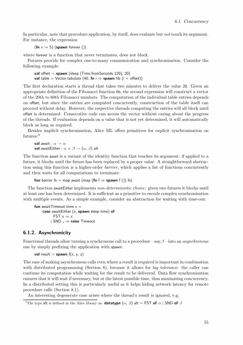
6.1. Concurrency
In particular, note that procedure application, by itself, does evaluate but not touch its argument.For instance, the expression
(fn x ⇒ 5) (spawn forever ())
where forever is a function that never terminates, does not block.Futures provide for complex one-to-many communication and synchronisation. Consider the
following example:
val offset = spawn (sleep (Time.fromSeconds 120); 20)val table = Vector.tabulate (40, fn i ⇒ spawn fib (i + offset))
The first declaration starts a thread that takes two minutes to deliver the value 20. Given anappropriate definition of the Fibonacci function fib, the second expression will construct a vectorof the 20th to 60th Fibonacci numbers. The computation of the individual table entries dependson offset, but since the entries are computed concurrently, construction of the table itself canproceed without delay. However, the respective threads computing the entries will all block untiloffset is determined. Consecutive code can access the vector without caring about the progressof the threads. If evaluation depends on a value that is not yet determined, it will automaticallyblock as long as required.
Besides implicit synchronisation, Alice ML offers primitives for explicit synchronisation onfutures:3
val await : α → αval awaitEither : α × β → (α, β) alt
The function await is a variant of the identity function that touches its argument: if applied to afuture, it blocks until the future has been replaced by a proper value. A straightforward abstrac-tion using this function is a higher-order barrier, which applies a list of functions concurrentlyand then waits for all computations to terminate:
fun barrier fs = map await (map (fn f ⇒ spawn f ()) fs)
The function awaitEither implements non-deterministic choice: given two futures it blocks untilat least one has been determined. It is sufficient as a primitive to encode complex synchronisationwith multiple events. As a simple example, consider an abstraction for waiting with time-out:
fun awaitTimeout time x =case awaitEither (x, spawn sleep time) of
FST x ⇒ x| SND ⇒ raise Timeout
6.1.2. Asynchronicity
Functional threads allow turning a synchronous call to a procedure – say, f – into an asynchronousone by simply prefixing the application with spawn:
val result = spawn f(x, y, z)
The ease of making asynchronous calls even where a result is required is important in combinationwith distributed programming (Section 8), because it allows for lag tolerance: the caller cancontinue its computation while waiting for the result to be delivered. Data flow synchronisationensures that it will wait if necessary, but at the latest possible time, thus maximising concurrency.In a distributed setting this is particularly useful as it helps hiding network latency for remoteprocedure calls (Section 8.1).
An interesting degenerate case arises where the thread’s result is ignored, e.g.
3The type alt is defined in the Alice library as: datatype (α, β) alt = FST of α | SND of β
55
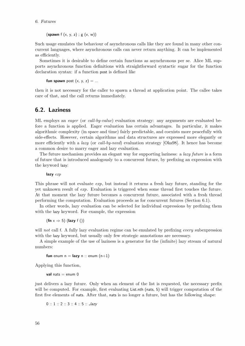
6. Futures
(spawn f (x, y, z) ; g (v, w))
Such usage emulates the behaviour of asynchronous calls like they are found in many other con-current languages, where asynchronous calls can never return anything. It can be implementedas efficiently.
Sometimes it is desirable to define certain functions as asynchronous per se. Alice ML sup-ports asynchronous function definitions with straightforward syntactic sugar for the functiondeclaration syntax: if a function post is defined like
fun spawn post (x, y, z) = ...
then it is not necessary for the caller to spawn a thread at application point. The callee takescare of that, and the call returns immediately.
6.2. Laziness
ML employs an eager (or call-by-value) evaluation strategy: any arguments are evaluated be-fore a function is applied. Eager evaluation has certain advantages. In particular, it makesalgorithmic complexity (in space and time) fairly predictable, and coexists more peacefully withside-effects. However, certain algorithms and data structures are expressed more elegantly ormore efficiently with a lazy (or call-by-need) evaluation strategy [Oka98]. It hence has becomea common desire to marry eager and lazy evaluation.
The future mechanism provides an elegant way for supporting laziness: a lazy future is a formof future that is introduced analogously to a concurrent future, by prefixing an expression withthe keyword lazy:
lazy exp
This phrase will not evaluate exp, but instead it returns a fresh lazy future, standing for theyet unknown result of exp. Evaluation is triggered when some thread first touches the future.At that moment the lazy future becomes a concurrent future, associated with a fresh threadperforming the computation. Evaluation proceeds as for concurrent futures (Section 6.1).
In other words, lazy evaluation can be selected for individual expressions by prefixing themwith the lazy keyword. For example, the expression
(fn x ⇒ 5) (lazy f ())
will not call f. A fully lazy evaluation regime can be emulated by prefixing every subexpressionwith the lazy keyword, but usually only few strategic annotations are necessary.
A simple example of the use of laziness is a generator for the (infinite) lazy stream of naturalnumbers:
fun enum n = lazy n :: enum (n+1)
Applying this function,
val nats = enum 0
just delivers a lazy future. Only when an element of the list is requested, the necessary prefixwill be computed. For example, first evaluating List.nth (nats, 5) will trigger computation of thefirst five elements of nats. After that, nats is no longer a future, but has the following shape:
0 :: 1 :: 2 :: 3 :: 4 :: 5 :: lazy
56
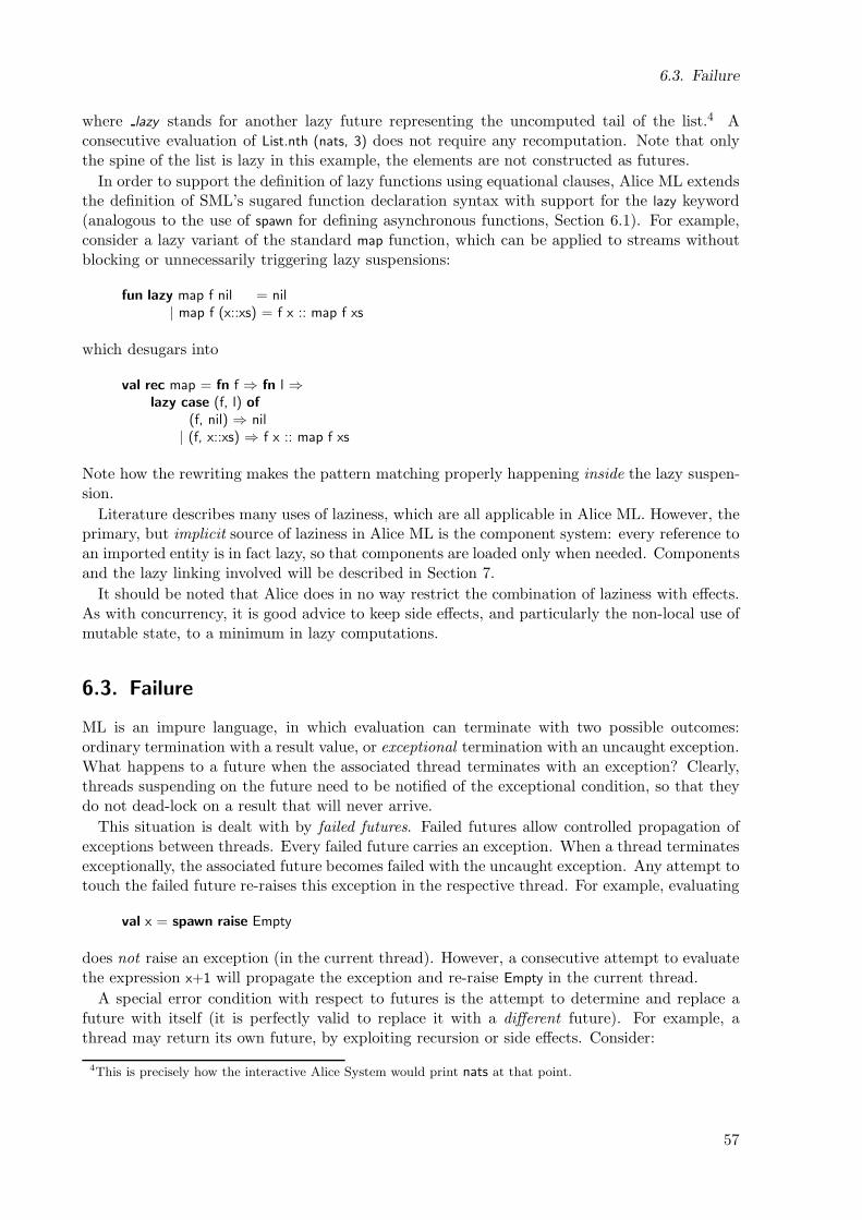
6.3. Failure
where lazy stands for another lazy future representing the uncomputed tail of the list.4 Aconsecutive evaluation of List.nth (nats, 3) does not require any recomputation. Note that onlythe spine of the list is lazy in this example, the elements are not constructed as futures.
In order to support the definition of lazy functions using equational clauses, Alice ML extendsthe definition of SML’s sugared function declaration syntax with support for the lazy keyword(analogous to the use of spawn for defining asynchronous functions, Section 6.1). For example,consider a lazy variant of the standard map function, which can be applied to streams withoutblocking or unnecessarily triggering lazy suspensions:
fun lazy map f nil = nil| map f (x::xs) = f x :: map f xs
which desugars into
val rec map = fn f ⇒ fn l ⇒lazy case (f, l) of
(f, nil) ⇒ nil| (f, x::xs) ⇒ f x :: map f xs
Note how the rewriting makes the pattern matching properly happening inside the lazy suspen-sion.
Literature describes many uses of laziness, which are all applicable in Alice ML. However, theprimary, but implicit source of laziness in Alice ML is the component system: every reference toan imported entity is in fact lazy, so that components are loaded only when needed. Componentsand the lazy linking involved will be described in Section 7.
It should be noted that Alice does in no way restrict the combination of laziness with effects.As with concurrency, it is good advice to keep side effects, and particularly the non-local use ofmutable state, to a minimum in lazy computations.
6.3. Failure
ML is an impure language, in which evaluation can terminate with two possible outcomes:ordinary termination with a result value, or exceptional termination with an uncaught exception.What happens to a future when the associated thread terminates with an exception? Clearly,threads suspending on the future need to be notified of the exceptional condition, so that theydo not dead-lock on a result that will never arrive.
This situation is dealt with by failed futures. Failed futures allow controlled propagation ofexceptions between threads. Every failed future carries an exception. When a thread terminatesexceptionally, the associated future becomes failed with the uncaught exception. Any attempt totouch the failed future re-raises this exception in the respective thread. For example, evaluating
val x = spawn raise Empty
does not raise an exception (in the current thread). However, a consecutive attempt to evaluatethe expression x+1 will propagate the exception and re-raise Empty in the current thread.
A special error condition with respect to futures is the attempt to determine and replace afuture with itself (it is perfectly valid to replace it with a different future). For example, athread may return its own future, by exploiting recursion or side effects. Consider:
4This is precisely how the interactive Alice System would print nats at that point.
57
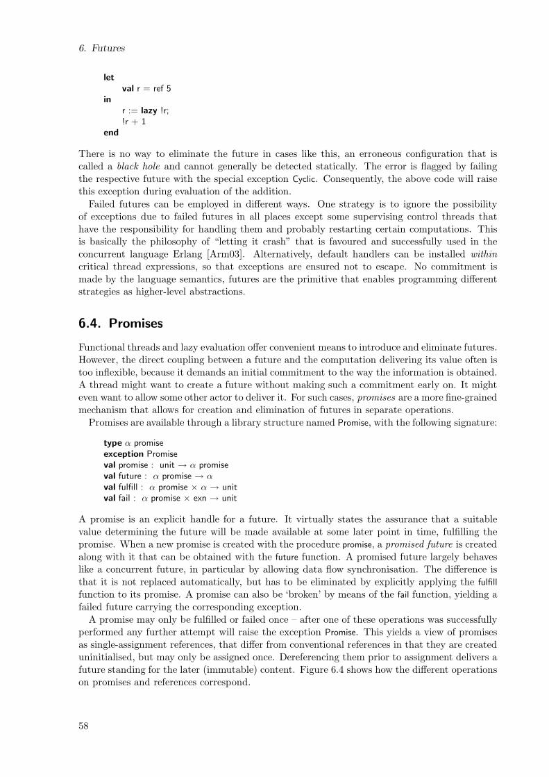
6. Futures
let
val r = ref 5in
r := lazy !r;!r + 1
end
There is no way to eliminate the future in cases like this, an erroneous configuration that iscalled a black hole and cannot generally be detected statically. The error is flagged by failingthe respective future with the special exception Cyclic. Consequently, the above code will raisethis exception during evaluation of the addition.
Failed futures can be employed in different ways. One strategy is to ignore the possibilityof exceptions due to failed futures in all places except some supervising control threads thathave the responsibility for handling them and probably restarting certain computations. Thisis basically the philosophy of “letting it crash” that is favoured and successfully used in theconcurrent language Erlang [Arm03]. Alternatively, default handlers can be installed withincritical thread expressions, so that exceptions are ensured not to escape. No commitment ismade by the language semantics, futures are the primitive that enables programming differentstrategies as higher-level abstractions.
6.4. Promises
Functional threads and lazy evaluation offer convenient means to introduce and eliminate futures.However, the direct coupling between a future and the computation delivering its value often istoo inflexible, because it demands an initial commitment to the way the information is obtained.A thread might want to create a future without making such a commitment early on. It mighteven want to allow some other actor to deliver it. For such cases, promises are a more fine-grainedmechanism that allows for creation and elimination of futures in separate operations.
Promises are available through a library structure named Promise, with the following signature:
type α promiseexception Promiseval promise : unit → α promiseval future : α promise → αval fulfill : α promise × α → unitval fail : α promise × exn → unit
A promise is an explicit handle for a future. It virtually states the assurance that a suitablevalue determining the future will be made available at some later point in time, fulfilling thepromise. When a new promise is created with the procedure promise, a promised future is createdalong with it that can be obtained with the future function. A promised future largely behaveslike a concurrent future, in particular by allowing data flow synchronisation. The difference isthat it is not replaced automatically, but has to be eliminated by explicitly applying the fulfill
function to its promise. A promise can also be ‘broken’ by means of the fail function, yielding afailed future carrying the corresponding exception.
A promise may only be fulfilled or failed once – after one of these operations was successfullyperformed any further attempt will raise the exception Promise. This yields a view of promisesas single-assignment references, that differ from conventional references in that they are createduninitialised, but may only be assigned once. Dereferencing them prior to assignment delivers afuture standing for the later (immutable) content. Figure 6.4 shows how the different operationson promises and references correspond.
58
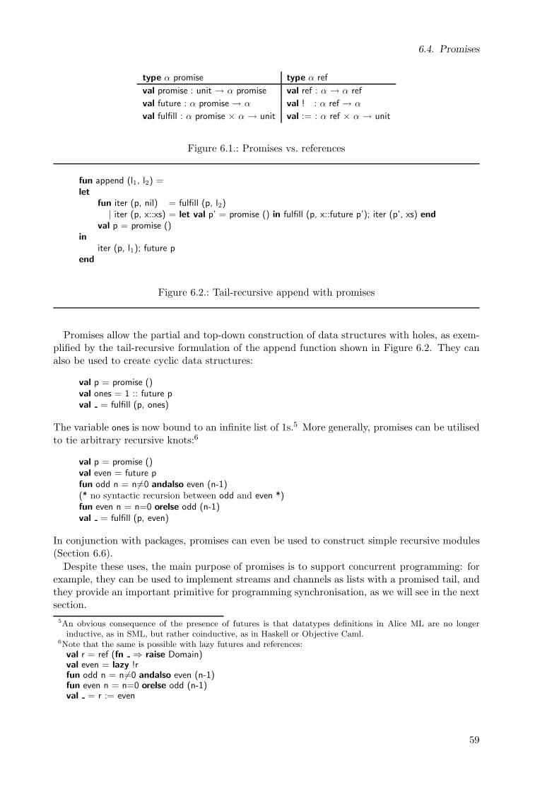
6.4. Promises
type α promise type α ref
val promise : unit → α promise val ref : α → α ref
val future : α promise → α val ! : α ref → α
val fulfill : α promise × α → unit val := : α ref × α → unit
Figure 6.1.: Promises vs. references
fun append (l1, l2) =let
fun iter (p, nil) = fulfill (p, l2)| iter (p, x::xs) = let val p’ = promise () in fulfill (p, x::future p’); iter (p’, xs) end
val p = promise ()in
iter (p, l1); future pend
Figure 6.2.: Tail-recursive append with promises
Promises allow the partial and top-down construction of data structures with holes, as exem-plified by the tail-recursive formulation of the append function shown in Figure 6.2. They canalso be used to create cyclic data structures:
val p = promise ()val ones = 1 :: future pval = fulfill (p, ones)
The variable ones is now bound to an infinite list of 1s.5 More generally, promises can be utilisedto tie arbitrary recursive knots:6
val p = promise ()val even = future pfun odd n = n6=0 andalso even (n-1)(* no syntactic recursion between odd and even *)fun even n = n=0 orelse odd (n-1)val = fulfill (p, even)
In conjunction with packages, promises can even be used to construct simple recursive modules(Section 6.6).
Despite these uses, the main purpose of promises is to support concurrent programming: forexample, they can be used to implement streams and channels as lists with a promised tail, andthey provide an important primitive for programming synchronisation, as we will see in the nextsection.
5An obvious consequence of the presence of futures is that datatypes definitions in Alice ML are no longerinductive, as in SML, but rather coinductive, as in Haskell or Objective Caml.
6Note that the same is possible with lazy futures and references:val r = ref (fn ⇒ raise Domain)val even = lazy !rfun odd n = n6=0 andalso even (n-1)fun even n = n=0 orelse odd (n-1)val = r := even
59
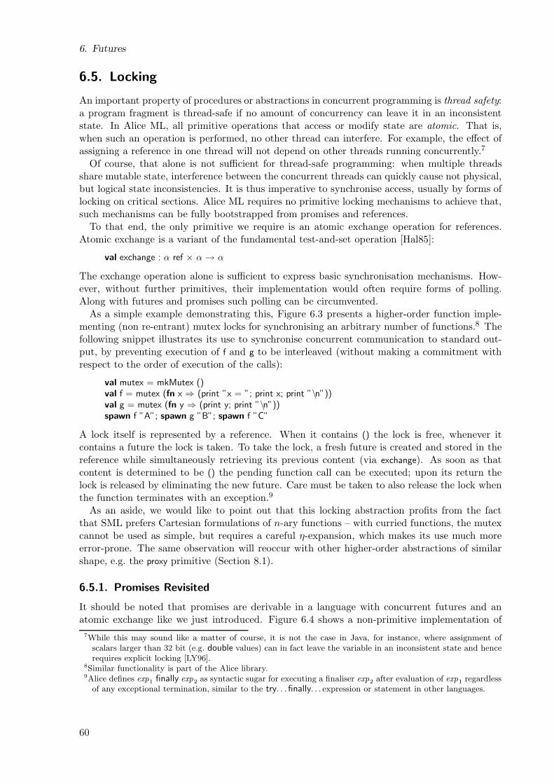
6. Futures
6.5. Locking
An important property of procedures or abstractions in concurrent programming is thread safety:a program fragment is thread-safe if no amount of concurrency can leave it in an inconsistentstate. In Alice ML, all primitive operations that access or modify state are atomic. That is,when such an operation is performed, no other thread can interfere. For example, the effect ofassigning a reference in one thread will not depend on other threads running concurrently.7
Of course, that alone is not sufficient for thread-safe programming: when multiple threadsshare mutable state, interference between the concurrent threads can quickly cause not physical,but logical state inconsistencies. It is thus imperative to synchronise access, usually by forms oflocking on critical sections. Alice ML requires no primitive locking mechanisms to achieve that,such mechanisms can be fully bootstrapped from promises and references.
To that end, the only primitive we require is an atomic exchange operation for references.Atomic exchange is a variant of the fundamental test-and-set operation [Hal85]:
val exchange : α ref × α → α
The exchange operation alone is sufficient to express basic synchronisation mechanisms. How-ever, without further primitives, their implementation would often require forms of polling.Along with futures and promises such polling can be circumvented.
As a simple example demonstrating this, Figure 6.3 presents a higher-order function imple-menting (non re-entrant) mutex locks for synchronising an arbitrary number of functions.8 Thefollowing snippet illustrates its use to synchronise concurrent communication to standard out-put, by preventing execution of f and g to be interleaved (without making a commitment withrespect to the order of execution of the calls):
val mutex = mkMutex ()val f = mutex (fn x ⇒ (print ”x = ”; print x; print ”\n”))val g = mutex (fn y ⇒ (print y; print ”\n”))spawn f ”A”; spawn g ”B”; spawn f ”C”
A lock itself is represented by a reference. When it contains () the lock is free, whenever itcontains a future the lock is taken. To take the lock, a fresh future is created and stored in thereference while simultaneously retrieving its previous content (via exchange). As soon as thatcontent is determined to be () the pending function call can be executed; upon its return thelock is released by eliminating the new future. Care must be taken to also release the lock whenthe function terminates with an exception.9
As an aside, we would like to point out that this locking abstraction profits from the factthat SML prefers Cartesian formulations of n-ary functions – with curried functions, the mutexcannot be used as simple, but requires a careful η-expansion, which makes its use much moreerror-prone. The same observation will reoccur with other higher-order abstractions of similarshape, e.g. the proxy primitive (Section 8.1).
6.5.1. Promises Revisited
It should be noted that promises are derivable in a language with concurrent futures and anatomic exchange like we just introduced. Figure 6.4 shows a non-primitive implementation of
7While this may sound like a matter of course, it is not the case in Java, for instance, where assignment ofscalars larger than 32 bit (e.g. double values) can in fact leave the variable in an inconsistent state and hencerequires explicit locking [LY96].
8Similar functionality is part of the Alice library.9Alice defines exp1 finally exp2 as syntactic sugar for executing a finaliser exp2 after evaluation of exp1 regardless
of any exceptional termination, similar to the try. . .finally. . . expression or statement in other languages.
60
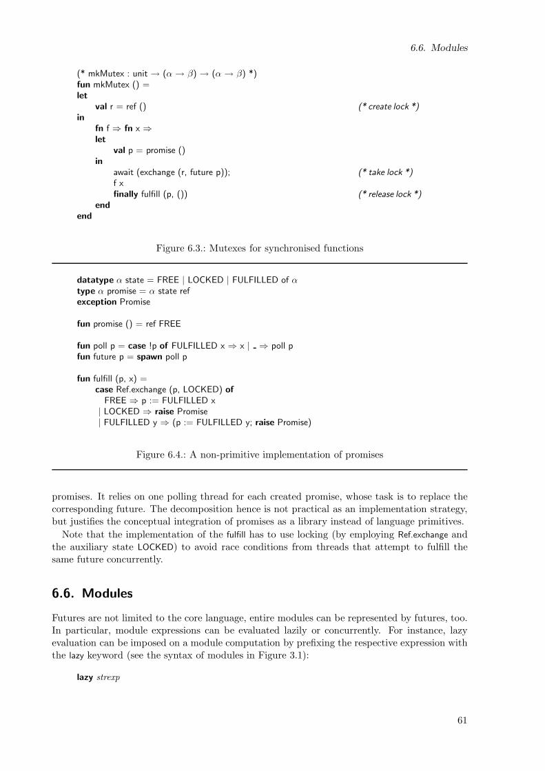
6.6. Modules
(* mkMutex : unit → (α → β) → (α → β) *)fun mkMutex () =let
val r = ref () (* create lock *)in
fn f ⇒ fn x ⇒let
val p = promise ()in
await (exchange (r, future p)); (* take lock *)f xfinally fulfill (p, ()) (* release lock *)
end
end
Figure 6.3.: Mutexes for synchronised functions
datatype α state = FREE | LOCKED | FULFILLED of αtype α promise = α state refexception Promise
fun promise () = ref FREE
fun poll p = case !p of FULFILLED x ⇒ x | ⇒ poll pfun future p = spawn poll p
fun fulfill (p, x) =case Ref.exchange (p, LOCKED) of
FREE ⇒ p := FULFILLED x| LOCKED ⇒ raise Promise| FULFILLED y ⇒ (p := FULFILLED y; raise Promise)
Figure 6.4.: A non-primitive implementation of promises
promises. It relies on one polling thread for each created promise, whose task is to replace thecorresponding future. The decomposition hence is not practical as an implementation strategy,but justifies the conceptual integration of promises as a library instead of language primitives.
Note that the implementation of the fulfill has to use locking (by employing Ref.exchange andthe auxiliary state LOCKED) to avoid race conditions from threads that attempt to fulfill thesame future concurrently.
6.6. Modules
Futures are not limited to the core language, entire modules can be represented by futures, too.In particular, module expressions can be evaluated lazily or concurrently. For instance, lazyevaluation can be imposed on a module computation by prefixing the respective expression withthe lazy keyword (see the syntax of modules in Figure 3.1):
lazy strexp
61
6. Futures
Concurrent evaluation of modules using spawn is available analogously. Lazy modules are some-times useful to perform functor applications lazily. However, the main importance of futureswith respect to modules lies in the central role they play for the Alice ML component system(Chapter 7): lazy module futures are ubiquitous as a consequence of the lazy linking mechanismfor components.
Like in the core language, a module future is touched by particular operations:
• Functor application touches the functor.
• Some primitive library functors touch some or all of their arguments.
• Applying certain primitive functions on packages (in particular pickling), touches the con-tained module.
It has to be stressed that projection from a structure (via a long identifier M.a) does not touchthe respective structure. That is, structure selection is implicitly lazy, and a structure is onlytouched if one if its fields is touched itself. Hence, evaluating a structure lazily defers evaluationof its body until one of its fields is needed. Consider:
structure M = lazy struct fun id x = x; val = print ”Now” end
val id = M.idval = print ”Not”val x = id 7
Merely evaluating M.id does not touch M, but applying it to an argument does – executing theabove program fragment prints ”NotNow”. The lazy semantics for structure projection naturallyextends to open declarations. It is motivated by the observation that structures are primarilyused to define local scopes and organise name spaces. It is not desirable that mere groupingand qualified naming changes strictness – otherwise modular programming would become anobstacle for laziness (and particularly lazy linking of components – Chapter 7).
Also note that creating and accessing packages (Chapter 4) does not per se touch the respectivemodule.
Module futures can be failed, e.g. if the module evaluation terminates with an exception.Exceptions from failed module futures can be caught because Alice ML allows modules to bedeclared in local scope (Section 3.2), which can be surrounded by a handler.
There are no promised module futures, but a module can be projected from a package (Chap-ter 4) that is a promised future, giving a similar effect. For example, we can create simplemutual recursion between modules:
val p = promise ()structure E = lazy unpack future p : sig val even : int → bool end
structure O = struct fun odd n = n6=0 andalso E.even (n-1) end
structure E = struct fun even n = n=0 orelse O.odd (n-1) end
val = fulfill (p, pack E : sig val even : int → bool end)
Note however, that any attempt to actually make type members mutually recursive will mostlikely result in a deadlock, because of the behaviour of type futures described below. More-over, the module’s signatures cannot be made mutually recursive. Hence, this approach is nosubstitute for a proper recursive module mechanism [Rus01, DHC01, Dre04].
6.7. Types
Types (which includes signatures) may reside in structures. The existence of module futureshence implies the existence of type futures. The notion of a type future is a novel concept that,
62
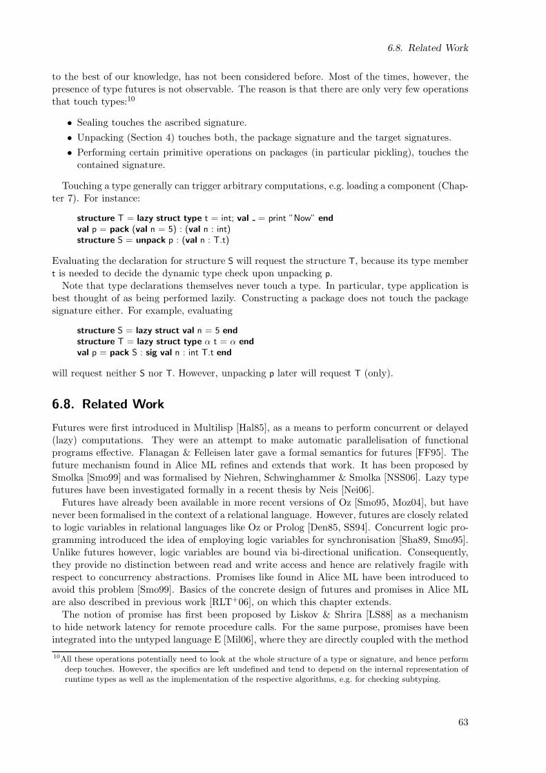
6.8. Related Work
to the best of our knowledge, has not been considered before. Most of the times, however, thepresence of type futures is not observable. The reason is that there are only very few operationsthat touch types:10
• Sealing touches the ascribed signature.
• Unpacking (Section 4) touches both, the package signature and the target signatures.
• Performing certain primitive operations on packages (in particular pickling), touches thecontained signature.
Touching a type generally can trigger arbitrary computations, e.g. loading a component (Chap-ter 7). For instance:
structure T = lazy struct type t = int; val = print ”Now” end
val p = pack (val n = 5) : (val n : int)structure S = unpack p : (val n : T.t)
Evaluating the declaration for structure S will request the structure T, because its type membert is needed to decide the dynamic type check upon unpacking p.
Note that type declarations themselves never touch a type. In particular, type application isbest thought of as being performed lazily. Constructing a package does not touch the packagesignature either. For example, evaluating
structure S = lazy struct val n = 5 end
structure T = lazy struct type α t = α end
val p = pack S : sig val n : int T.t end
will request neither S nor T. However, unpacking p later will request T (only).
6.8. Related Work
Futures were first introduced in Multilisp [Hal85], as a means to perform concurrent or delayed(lazy) computations. They were an attempt to make automatic parallelisation of functionalprograms effective. Flanagan & Felleisen later gave a formal semantics for futures [FF95]. Thefuture mechanism found in Alice ML refines and extends that work. It has been proposed bySmolka [Smo99] and was formalised by Niehren, Schwinghammer & Smolka [NSS06]. Lazy typefutures have been investigated formally in a recent thesis by Neis [Nei06].
Futures have already been available in more recent versions of Oz [Smo95, Moz04], but havenever been formalised in the context of a relational language. However, futures are closely relatedto logic variables in relational languages like Oz or Prolog [Den85, SS94]. Concurrent logic pro-gramming introduced the idea of employing logic variables for synchronisation [Sha89, Smo95].Unlike futures however, logic variables are bound via bi-directional unification. Consequently,they provide no distinction between read and write access and hence are relatively fragile withrespect to concurrency abstractions. Promises like found in Alice ML have been introduced toavoid this problem [Smo99]. Basics of the concrete design of futures and promises in Alice MLare also described in previous work [RLT+06], on which this chapter extends.
The notion of promise has first been proposed by Liskov & Shrira [LS88] as a mechanismto hide network latency for remote procedure calls. For the same purpose, promises have beenintegrated into the untyped language E [Mil06], where they are directly coupled with the method
10All these operations potentially need to look at the whole structure of a type or signature, and hence performdeep touches. However, the specifics are left undefined and tend to depend on the internal representation ofruntime types as well as the implementation of the respective algorithms, e.g. for checking subtyping.
63
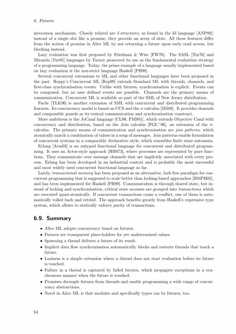
6. Futures
invocation mechanism. Closely related are I-structures, as found in the Id language [ANP89]:instead of a single slot like a promise, they provide an array of slots. All these features differfrom the notion of promise in Alice ML by not returning a future upon early read access, butblocking instead.
Lazy evaluation was first proposed by Friedman & Wise [FW76]. The SASL [Tur76] andMiranda [Tur85] languages by Turner pioneered its use as the fundamental evaluation strategyof a programming language. Today, the prime example of a language usually implemented basedon lazy evaluation is the non-strict language Haskell [PH99].
Several concurrent extensions to ML and other functional languages have been proposed inthe past. Reppy’s Concurrent ML [Rep99] extends Standard ML with threads, channels, andfirst-class synchronisation events. Unlike with futures, synchronisation is explicit. Events canbe composed, but no user defined events are possible. Channels are the primary means ofcommunication. Concurrent ML is available as part of the SML of New Jersey distribution.
Facile [TLK96] is another extension of SML with concurrent and distributed programmingfeatures. Its concurrency model is based on CCS and the π-calculus [Mil89]. It provides channelsand composable guards as its central communication and synchronisation construct.
More ambitious is the JoCaml language [CL99, FMS01], which extends Objective Caml withconcurrency and distribution, based on the Join calculus [FGL+96], an extension of the π-calculus. The primary means of communication and synchronisation are join patterns, whichatomically match a combination of values in a soup of messages. Join patterns enable formulationof concurrent systems in a comparably declarative style, which resembles finite state automata.
Erlang [Arm03] is an untyped functional language for concurrent and distributed program-ming. It uses an Actor-style approach [HBS73], where processes are represented by pure func-tions. They communicate over message channels that are implicitly associated with every pro-cess. Erlang has been developed in an industrial context and is probably the most successfuland most widely used concurrent functional language so far.
Lately, transactional memory has been proposed as an alternative, lock-free paradigm for con-current programming that is supposed to scale better than locking-based approaches [HMPH05],and has been implemented for Haskell [PH99]. Communication is through shared state, but in-stead of locking and synchronisation, critical state accesses are grouped into transactions whichare executed quasi-atomically. If concurrent transactions cause a conflict, one of them is auto-matically rolled back and retried. The approach benefits greatly from Haskell’s expressive typesystem, which allows to statically enforce purity of transactions.
6.9. Summary
• Alice ML adopts concurrency based on futures.
• Futures are transparent place-holders for yet undetermined values.
• Spawning a thread delivers a future of its result.
• Implicit data flow synchronisation automatically blocks and restarts threads that touch afuture.
• Laziness is a simple extension where a thread does not start evaluation before its futureis touched.
• Failure in a thread is captured by failed futures, which propagate exceptions in a syn-chronous manner when the future is touched.
• Promises decouple futures from threads and enable programming a wide range of concur-rency abstractions.
• Novel in Alice ML is that modules and specifically types can be futures, too.
64
7. Components
Software of non-trivial complexity can neither be developed nor deployed as a monolithic block.To keep the development process manageable, and to allow flexible installation and configu-ration, software has to be split into functional building blocks that can be created separately,configured dynamically, and even be exchanged between processes. Such building blocks arecalled components.
We distinguish components from modules: while modules provide logical separation, namespacing, genericity, and encapsulation, components provide physical separation and dynamiccomposition. Modules are referred to by identifiers and static scoping rules, where componentsare identified by extra-linguistic means that are resolved dynamically. Both mechanisms com-plement each other. More precisely, components contain modules. It is the component systemthat enables closing over free references in a module implementation and hence turning it intoa self-contained entity.
Alice ML incorporates a powerful notion of component that is a refinement and extension ofthe component system found in the Oz language1 [DKSS98], which in turn was partially inspiredby Modula-3 [BNOW95] and Java [GJS96]. It provides all of the following:
• Separate compilation. Components can be translated independently.
• Lazy dynamic linking. Loading can be performed automatically when needed.
• Type safety. Components carry strong type information and linking checks it.
• Subtyping. Type checking is tolerant against interface changes.
• Static linking. Components can be bundled into larger components off-line.
• Dynamic creation. Components can be computed and exported dynamically.
• Sandboxing. Custom component managers enable selective import policies.
The component system of Alice ML is based on a combination of different mechanisms pre-sented in the previous chapters:
• Higher-order modules (Chapter 3), for encapsulating all possible language entities,
• Packages (Chapter 4), for dynamic type checking of imports,
• Pickling (Chapter 5), for representing components externally,
• Futures (Chapter 6), for performing linking lazily.
Packages already allow dynamic loading and exchanging of modules. However, these moduleshave to be fully evaluated and closed. If we wanted to delay evaluation, or to have it dependon other modules, then we would have to resort to functional (or functorial) abstraction. Com-ponents provide a much more comfortable and flexible means for achieving the same effect.Nevertheless, in Section 7.6 we will see that they can actually be expressed as a – relativelysimple – functional abstraction. We will first present components as an independent featurebefore we show how precisely they relate to the mechanisms listed above.
1In Oz, components are called functors by slight abuse of terminology.
65
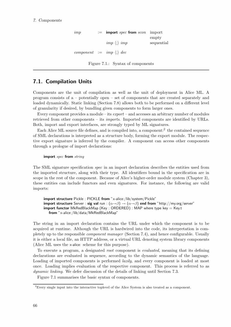
7. Components
imp := import spec from scon importempty
imp 〈;〉 imp sequential
component := imp 〈;〉 dec
Figure 7.1.: Syntax of components
7.1. Compilation Units
Components are the unit of compilation as well as the unit of deployment in Alice ML. Aprogram consists of a – potentially open – set of components that are created separately andloaded dynamically. Static linking (Section 7.8) allows both to be performed on a different levelof granularity if desired, by bundling given components to form larger ones.
Every component provides a module – its export – and accesses an arbitrary number of modulesretrieved from other components – its imports. Imported components are identified by URLs.Both, import and export interfaces, are strongly typed by ML signatures.
Each Alice ML source file defines, and is compiled into, a component:2 the contained sequenceof SML declarations is interpreted as a structure body, forming the export module. The respec-tive export signature is inferred by the compiler. A component can access other componentsthrough a prologue of import declarations:
import spec from string
The SML signature specification spec in an import declaration describes the entities used fromthe imported structure, along with their type. All identifiers bound in the specification are inscope in the rest of the component. Because of Alice’s higher-order module system (Chapter 3),these entities can include functors and even signatures. For instance, the following are validimports:
import structure Pickle : PICKLE from ”x-alice:/lib/system/Pickle”import structure Server : sig val run : (α→β) → (α→β) end from ”http://my.org/server”import functor MkRedBlackMap (Key : ORDERED) : MAP where type key = Key.t
from ”x-alice:/lib/data/MkRedBlackMap”
The string in an import declaration contains the URL under which the component is to beacquired at runtime. Although the URL is hardwired into the code, its interpretation is com-pletely up to the responsible component manager (Section 7.4), and hence configurable. Usuallyit is either a local file, an HTTP address, or a virtual URL denoting system library components(Alice ML uses the x-alice: scheme for this purpose).
To execute a program, a designated root component is evaluated, meaning that its definingdeclarations are evaluated in sequence, according to the dynamic semantics of the language.Loading of imported components is performed lazily, and every component is loaded at mostonce. Loading implies evaluation of the respective component. This process is referred to asdynamic linking. We defer discussion of the details of linking until Section 7.3.
Figure 7.1 summarises the basic syntax of components.
2Every single input into the interactive toplevel of the Alice System is also treated as a component.
66
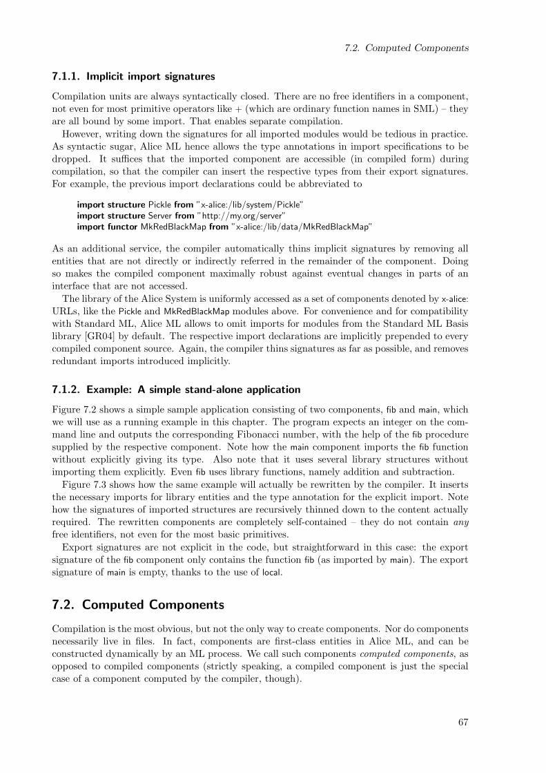
7.2. Computed Components
7.1.1. Implicit import signatures
Compilation units are always syntactically closed. There are no free identifiers in a component,not even for most primitive operators like + (which are ordinary function names in SML) – theyare all bound by some import. That enables separate compilation.
However, writing down the signatures for all imported modules would be tedious in practice.As syntactic sugar, Alice ML hence allows the type annotations in import specifications to bedropped. It suffices that the imported component are accessible (in compiled form) duringcompilation, so that the compiler can insert the respective types from their export signatures.For example, the previous import declarations could be abbreviated to
import structure Pickle from ”x-alice:/lib/system/Pickle”import structure Server from ”http://my.org/server”import functor MkRedBlackMap from ”x-alice:/lib/data/MkRedBlackMap”
As an additional service, the compiler automatically thins implicit signatures by removing allentities that are not directly or indirectly referred in the remainder of the component. Doingso makes the compiled component maximally robust against eventual changes in parts of aninterface that are not accessed.
The library of the Alice System is uniformly accessed as a set of components denoted by x-alice:
URLs, like the Pickle and MkRedBlackMap modules above. For convenience and for compatibilitywith Standard ML, Alice ML allows to omit imports for modules from the Standard ML Basislibrary [GR04] by default. The respective import declarations are implicitly prepended to everycompiled component source. Again, the compiler thins signatures as far as possible, and removesredundant imports introduced implicitly.
7.1.2. Example: A simple stand-alone application
Figure 7.2 shows a simple sample application consisting of two components, fib and main, whichwe will use as a running example in this chapter. The program expects an integer on the com-mand line and outputs the corresponding Fibonacci number, with the help of the fib proceduresupplied by the respective component. Note how the main component imports the fib functionwithout explicitly giving its type. Also note that it uses several library structures withoutimporting them explicitly. Even fib uses library functions, namely addition and subtraction.
Figure 7.3 shows how the same example will actually be rewritten by the compiler. It insertsthe necessary imports for library entities and the type annotation for the explicit import. Notehow the signatures of imported structures are recursively thinned down to the content actuallyrequired. The rewritten components are completely self-contained – they do not contain anyfree identifiers, not even for the most basic primitives.
Export signatures are not explicit in the code, but straightforward in this case: the exportsignature of the fib component only contains the function fib (as imported by main). The exportsignature of main is empty, thanks to the use of local.
7.2. Computed Components
Compilation is the most obvious, but not the only way to create components. Nor do componentsnecessarily live in files. In fact, components are first-class entities in Alice ML, and can beconstructed dynamically by an ML process. We call such components computed components, asopposed to compiled components (strictly speaking, a compiled component is just the specialcase of a component computed by the compiler, though).
67
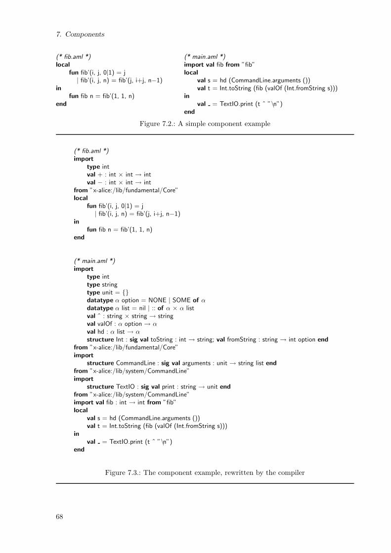
7. Components
(* fib.aml *)local
fun fib’(i, j, 0|1) = j| fib’(i, j, n) = fib’(j, i+j, n−1)
in
fun fib n = fib’(1, 1, n)end
(* main.aml *)import val fib from ”fib”local
val s = hd (CommandLine.arguments ())val t = Int.toString (fib (valOf (Int.fromString s)))
in
val = TextIO.print (t ˆ ”\n”)end
Figure 7.2.: A simple component example
(* fib.aml *)import
type intval + : int × int → intval − : int × int → int
from ”x-alice:/lib/fundamental/Core”local
fun fib’(i, j, 0|1) = j| fib’(i, j, n) = fib’(j, i+j, n−1)
in
fun fib n = fib’(1, 1, n)end
(* main.aml *)import
type inttype stringtype unit = datatype α option = NONE | SOME of αdatatype α list = nil | :: of α × α listval ˆ : string × string → stringval valOf : α option → αval hd : α list → αstructure Int : sig val toString : int → string; val fromString : string → int option end
from ”x-alice:/lib/fundamental/Core”import
structure CommandLine : sig val arguments : unit → string list end
from ”x-alice:/lib/system/CommandLine”import
structure TextIO : sig val print : string → unit end
from ”x-alice:/lib/system/CommandLine”import val fib : int → int from ”fib”local
val s = hd (CommandLine.arguments ())val t = Int.toString (fib (valOf (Int.fromString s)))
in
val = TextIO.print (t ˆ ”\n”)end
Figure 7.3.: The component example, rewritten by the compiler
68
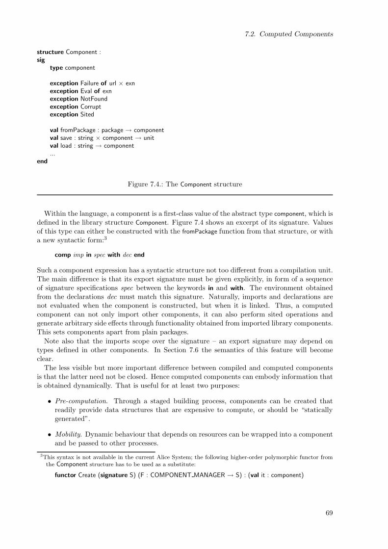
7.2. Computed Components
structure Component :sig
type component
exception Failure of url × exnexception Eval of exnexception NotFoundexception Corruptexception Sited
val fromPackage : package → componentval save : string × component → unitval load : string → component...
end
Figure 7.4.: The Component structure
Within the language, a component is a first-class value of the abstract type component, which isdefined in the library structure Component. Figure 7.4 shows an excerpt of its signature. Valuesof this type can either be constructed with the fromPackage function from that structure, or witha new syntactic form:3
comp imp in spec with dec end
Such a component expression has a syntactic structure not too different from a compilation unit.The main difference is that its export signature must be given explicitly, in form of a sequenceof signature specifications spec between the keywords in and with. The environment obtainedfrom the declarations dec must match this signature. Naturally, imports and declarations arenot evaluated when the component is constructed, but when it is linked. Thus, a computedcomponent can not only import other components, it can also perform sited operations andgenerate arbitrary side effects through functionality obtained from imported library components.This sets components apart from plain packages.
Note also that the imports scope over the signature – an export signature may depend ontypes defined in other components. In Section 7.6 the semantics of this feature will becomeclear.
The less visible but more important difference between compiled and computed componentsis that the latter need not be closed. Hence computed components can embody information thatis obtained dynamically. That is useful for at least two purposes:
• Pre-computation. Through a staged building process, components can be created thatreadily provide data structures that are expensive to compute, or should be “staticallygenerated”.
• Mobility. Dynamic behaviour that depends on resources can be wrapped into a componentand be passed to other processes.
3This syntax is not available in the current Alice System; the following higher-order polymorphic functor fromthe Component structure has to be used as a substitute:
functor Create (signature S) (F : COMPONENT MANAGER → S) : (val it : component)
69
7. Components
Pre-computation already is enabled to a certain degree by packages and persistence (Sec-tion 4.2). However, packages are relatively limited: as pickles, they have to be closed, i.e. theycannot make use of any library functionality local to the site where they are loaded. In partic-ular, they cannot easily provide behaviour that requires access to resources – e.g. input/output– because such resources and operations on them cannot be stored in pickles (Section 5.3).Components come to the rescue.
To demonstrate the utility of computed components, consider the example of a simple HelloWorld application. The following program computes a component that exports a function thatprints a message containing the component’s date of creation when invoked later:
val date = Date.toString (Date.fromTimeLocal (Time.now ()))val component =
comp
import structure TextIO from ”x-alice:/lib/system/TextIO”in
val hello : unit → unitwith
fun hello () = TextIO.print (”Hello world! Created at ” ˆ date ˆ ”\n”)end
val = Component.save (”hello”, component)
Note that date is computed outside the component, and hence included as a value. Component.save
pickles a computed component to a file. Component files created this way behave exactly likecomponents created by the compiler, they can be loaded or imported. For example, the simplestpossible program utilising the component created above is the following:
import val hello : unit → unit from ”hello”val = hello ()
Alternatively, we can use Component.load to load it as a first-class value, but it then requires anexplicit component manager (Section 7.4) to evaluate it.
Packages can be directly converted to components with the Component.fromPackage function,which is sometimes convenient – we speak of evaluated components in this case, because theyjust export a constant module value. However, the key difference between a component and asimple package is that a component enables import of resources and other functionality local tothe target site. As the example shows, computed components can thus have arbitrary, ‘impure’behaviour, but are yet mobile, i.e. exportable through pickling. For instance, the example wouldnot work if we omitted the import declaration for TextIO – then the local instance of TextIO.print
would be in the closure of component, and pickling would fail with a Sited exception because print
is a resourceful operation (Section 5.3). With the import, we effectively enforce rebinding of allscoped references to TextIO on the target site. However, the target site may choose to preventthe import if it wishes to restrict the capabilities of an untrusted component (Section 7.5).
Rebinding is particularly important for distributed programming. Exchanging dynamic be-haviour between processes can be achieved by creating a mobile component serving two purposes:
• it closes over all entities obtained at creation site, thus containing the necessary dynamicinformation (like date above),
• it abstracts over all entities to be obtained at the target site, thus enabling pickling and(re)binding (like TextIO above).
The former is handled automatically by closure and the semantics of pickling. The latter canbe controlled by the use of import declarations in the definition of the mobile component. The
70
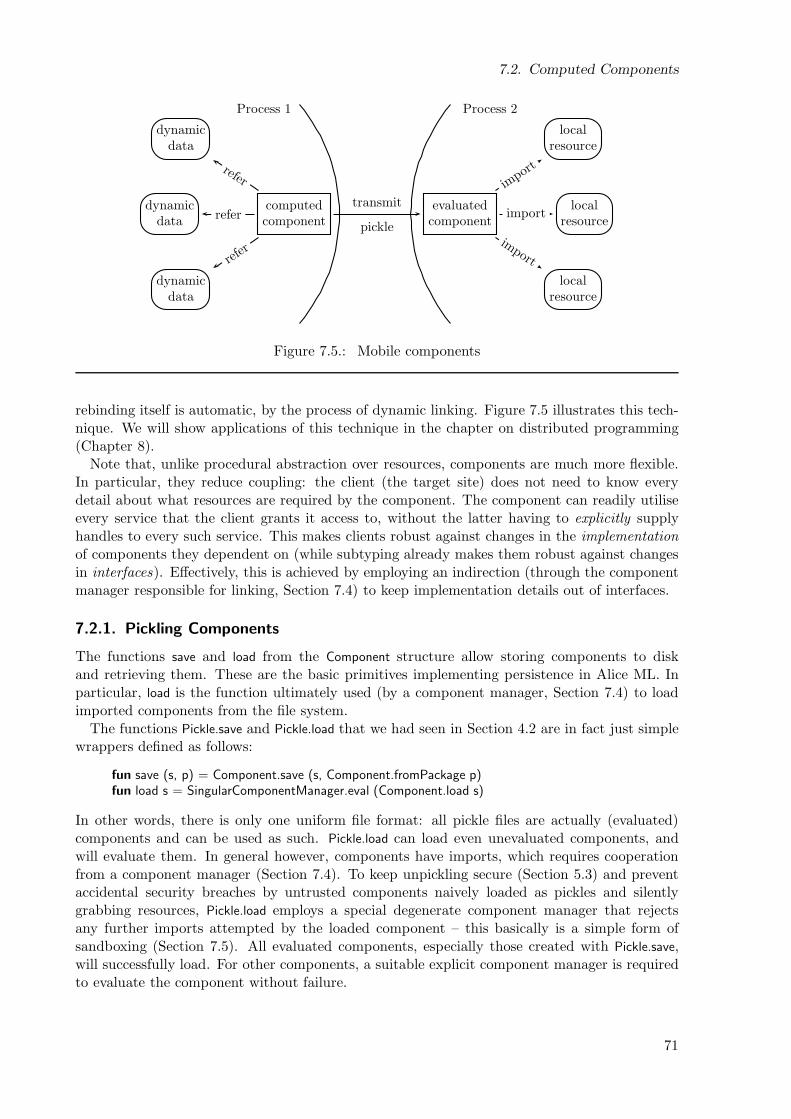
7.2. Computed Components
dynamicdata
dynamicdata
dynamicdata
computedcomponent
evaluatedcomponent
localresource
localresource
localresource
refer
refer
refer
transmit
pickle
impo
rt
import
import
Process 1 Process 2
Figure 7.5.: Mobile components
rebinding itself is automatic, by the process of dynamic linking. Figure 7.5 illustrates this tech-nique. We will show applications of this technique in the chapter on distributed programming(Chapter 8).
Note that, unlike procedural abstraction over resources, components are much more flexible.In particular, they reduce coupling: the client (the target site) does not need to know everydetail about what resources are required by the component. The component can readily utiliseevery service that the client grants it access to, without the latter having to explicitly supplyhandles to every such service. This makes clients robust against changes in the implementationof components they dependent on (while subtyping already makes them robust against changesin interfaces). Effectively, this is achieved by employing an indirection (through the componentmanager responsible for linking, Section 7.4) to keep implementation details out of interfaces.
7.2.1. Pickling Components
The functions save and load from the Component structure allow storing components to diskand retrieving them. These are the basic primitives implementing persistence in Alice ML. Inparticular, load is the function ultimately used (by a component manager, Section 7.4) to loadimported components from the file system.
The functions Pickle.save and Pickle.load that we had seen in Section 4.2 are in fact just simplewrappers defined as follows:
fun save (s, p) = Component.save (s, Component.fromPackage p)fun load s = SingularComponentManager.eval (Component.load s)
In other words, there is only one uniform file format: all pickle files are actually (evaluated)components and can be used as such. Pickle.load can load even unevaluated components, andwill evaluate them. In general however, components have imports, which requires cooperationfrom a component manager (Section 7.4). To keep unpickling secure (Section 5.3) and preventaccidental security breaches by untrusted components naively loaded as pickles and silentlygrabbing resources, Pickle.load employs a special degenerate component manager that rejectsany further imports attempted by the loaded component – this basically is a simple form ofsandboxing (Section 7.5). All evaluated components, especially those created with Pickle.save,will successfully load. For other components, a suitable explicit component manager is requiredto evaluate the component without failure.
71
7. Components
7.3. Dynamic Linking
The components making up an application form a directed graph with respect to their importdependencies. A designated root is the main component of a program. Primitive library com-ponents providing system services and the most basic functionality make up the leaves of thegraph.
To execute a program, its root component is evaluated. For compiled components, this meansthat the respective declarations are evaluated in sequence. As already explained, loading ofimported components is performed lazily, and every component is loaded and evaluated onlyonce. This is achieved by treating every cross-component reference as a lazy future (Section 6.2).Conceptually, the lazy thread suspended by the future is responsible for loading the componentwhen it is touched.
The process of loading and evaluating a component requested as import (by another compo-nent) is referred to as dynamic linking. Linking a component involves several steps:
1. Resolution. The import URL is normalised relative to the URL of the current component.
2. Acquisition. If that URL is being requested for the first time, it is loaded.
3. Evaluation. If the component has been loaded afresh, its body is evaluated and itsdynamic export signature computed.
4. Type Checking. The component’s export signature is matched against the respectiveimport signature.
Each of the steps can fail: for instance, the component might be inaccessible or malformed,evaluation may terminate with an exception, or type checking may discover a mismatch. Undereach of these circumstances, all futures representing references to the component are failed(Section 6.3) with the standard exception Component.Failure (Figure 7.4):
exception Failure of url × exn
The URL denotes the requested component and the nested exception describes the precise causeof the failure. In particular, it can be an I/O exception, the exception Unpack (Section 4.1),or any of the following exceptions, which are also defined in the library structure Component
(Figure 7.4):
exception NotFound (* component was not found *)exception Corrupt (* component is malformed *)exception Eval of exn (* component evaluation terminated with an exception *)
In the case of Eval, the uncaught exception is in turn nested.
Note that the import graph of a program may contain cycles. In the extreme, a componentmay even import itself, although this is hardly useful. Thanks to lazy linking, cycles pose noproblem as long as at least one of the components on the cycle does not need its respectiveimport immediately. Otherwise a deadlock may occur. In practice, cyclic imports are very rare.Programs typically rely on implicit import signatures inserted by the compiler (Section 7.1). Byconstruction, such imports can never be cyclic, unless some of the components are changed andrecompiled during the build process.4
4A trick that also works in Java.
72
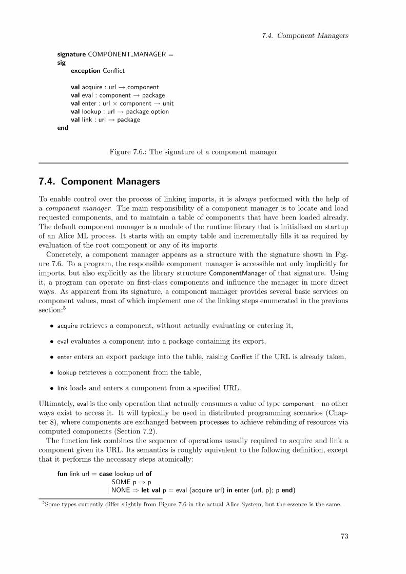
7.4. Component Managers
signature COMPONENT MANAGER =sig
exception Conflict
val acquire : url → componentval eval : component → packageval enter : url × component → unitval lookup : url → package optionval link : url → package
end
Figure 7.6.: The signature of a component manager
7.4. Component Managers
To enable control over the process of linking imports, it is always performed with the help ofa component manager. The main responsibility of a component manager is to locate and loadrequested components, and to maintain a table of components that have been loaded already.The default component manager is a module of the runtime library that is initialised on startupof an Alice ML process. It starts with an empty table and incrementally fills it as required byevaluation of the root component or any of its imports.
Concretely, a component manager appears as a structure with the signature shown in Fig-ure 7.6. To a program, the responsible component manager is accessible not only implicitly forimports, but also explicitly as the library structure ComponentManager of that signature. Usingit, a program can operate on first-class components and influence the manager in more directways. As apparent from its signature, a component manager provides several basic services oncomponent values, most of which implement one of the linking steps enumerated in the previoussection:5
• acquire retrieves a component, without actually evaluating or entering it,
• eval evaluates a component into a package containing its export,
• enter enters an export package into the table, raising Conflict if the URL is already taken,
• lookup retrieves a component from the table,
• link loads and enters a component from a specified URL.
Ultimately, eval is the only operation that actually consumes a value of type component – no otherways exist to access it. It will typically be used in distributed programming scenarios (Chap-ter 8), where components are exchanged between processes to achieve rebinding of resources viacomputed components (Section 7.2).
The function link combines the sequence of operations usually required to acquire and link acomponent given its URL. Its semantics is roughly equivalent to the following definition, exceptthat it performs the necessary steps atomically:
fun link url = case lookup url of
SOME p ⇒ p| NONE ⇒ let val p = eval (acquire url) in enter (url, p); p end)
5Some types currently differ slightly from Figure 7.6 in the actual Alice System, but the essence is the same.
73

7. Components
Note that there is no operation to remove a component from the table. While this is not apre-requisite for achieving soundness – thanks to typing being based on generative type names– it is a desirable property of a component manager to grow monotonically, in order to maintainthe property that every component is evaluated only once. If required, unloading of componentscan be simulated by creating a child component manager (Section 7.5), link a component withit, and then drop all references to it [Kor06].
7.5. Resources and Sandboxing
The relevance of component managers lies in their ability to control imports. That ability canbe utilised to realise security measures. In an open setting it is important to handle untrustedcomponents, and to restrict their capabilities. For example, not all components should be givenunrestricted access to the local file system.
To deal with this, component managers can be employed to adopt the approach taken byJava: they can form a sandbox to execute untrusted components in. Sandboxing relies on threefactors:
• Sited Resources. All critical operations and other objects that provide access to effectfulservices (e.g. input/output, system calls, various runtime services) are considered resources(Section 5.3). Resources cannot be pickled, hence there is no way to export them froma process. Consequently, no component imported into a process can contain any directreference to resources.
• Resource Acquisition through Component Managers. The only way a componentcan gain access to resources is by importing them from so-called primitive components onthe local site. Because all imports are controlled by a component manager, and primitivecomponents are identified by a stable naming scheme, the responsible manager can thusdecide what access to grant a given component.
• Custom Managers. It is possible to create custom managers that restrict the access tocertain components and explicitly link untrusted components through them. A componentmanager is inherited, i.e. all imports directly or indirectly requested by a component willbe linked using the same manager (or another custom manager that can only be definedin terms of that manager).
In other words, every component initially receives an (implicit) reference to exactly one resource:its component manager. It is then the responsibility of this manager to decide what furtherresources, and hence capabilities, are given to the component or its descendants.
The initial manager starting up an Alice process usually provides access to all resources. Theresourceful primitive components made available by this manager are an integral part of theruntime system and do not exist independently from it.
On the language level, a custom manager simply is a user-defined implementation of theCOMPONENT MANAGER signature. For example, the Alice ML library provides a functor tocreate new managers with specialised behaviour. When a custom manager is created, then itcan only use capabilities provided by its own ‘parent’ manager. In particular, the only way toprovide access to primitive components is by forwarding the respective requests to the parentmanager. Hence a custom manager can never grant more access than it has itself. Thus there isno way to bypass the restrictions of a manager – a custom manager represents a proper sandbox.
There are several possible ways in which a custom manager can restrict access:
74
7.6. Decomposition of the Component System
• It can simply reject loading from specific system URLs altogether, and only forward re-quests it deems save.
• It can restrict the signature under which specific components are made available, by for-warding the request to its parent manager, but repackaging the result with a thinnersignature (e.g. removing the operations for opening output files from TextIO).
• It can substitute critical components by security-sensitive wrappers, that dynamicallycheck access per operation, using fine-grained policies (this corresponds to Java’s SecurityManager).
For Alice ML, either of these approaches is feasible and programmable. So far, the Alice MLlibrary provides only minimal infrastructure for setting up custom managers. A thorough anal-ysis of the design space is independent of language design issues as discussed here, and thus leftfor future work. However, the language semantics provide all necessary prerequisites.
Scharfstein describes one possible design and implementation of a sandboxing library for AliceML [Sch06], which uses secure wrapper components performing dynamic checks with respect touser-configurable policies, but also enables the user of the sandbox to plug in her own behaviour.Noteworthily, sandboxing is realised fully within the language itself and does not require anydirect support from the core system.
We should stress again that security is not the focus of this thesis, and that the above descrip-tion is only meant to show that Alice ML is potentially secure. We do not claim to describe anend-to-end security concept. Nor does the current implementation of the language provide it.
7.6. Decomposition of the Component System
At first, components may look like a complex mechanism. In this section we will refute thispresumption, by giving a simple reduction of components to functions and packages. The meritof this reduction is three-fold:
• It keeps the language conceptually simple.
• It defines component semantics without need for additional technical machinery.
• Soundness and related properties follow for free.
The close relation between components and the concepts presented in previous chapters –like modules, packages and futures – is obvious, so one might hope that there exists a simplereduction. And indeed, components can be understood as mere syntactic sugar.
7.6.1. Components
A component can be seen as a function that evaluates to a package (Chapter 4). The packageencapsulates the export module and its signature.
More precisely, the abstract type component can be implemented as a higher-order functiontype:
type component = (url → package) → package
Its argument encapsulates the component manager, needed to acquire imports. Supplying thefunction evaluates the component.
Accordingly, a component expression
75
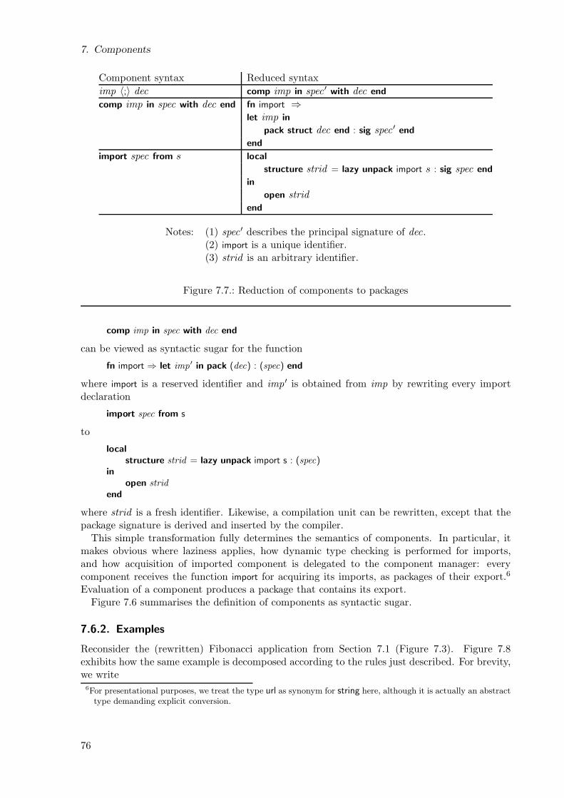
7. Components
Component syntax Reduced syntax
imp 〈;〉 dec comp imp in spec ′ with dec end
comp imp in spec with dec end fn import ⇒let imp in
pack struct dec end : sig spec ′ end
end
import spec from s local
structure strid = lazy unpack import s : sig spec end
in
open stridend
Notes: (1) spec ′ describes the principal signature of dec.(2) import is a unique identifier.(3) strid is an arbitrary identifier.
Figure 7.7.: Reduction of components to packages
comp imp in spec with dec end
can be viewed as syntactic sugar for the function
fn import ⇒ let imp′ in pack (dec) : (spec) end
where import is a reserved identifier and imp ′ is obtained from imp by rewriting every importdeclaration
import spec from s
to
local
structure strid = lazy unpack import s : (spec)in
open stridend
where strid is a fresh identifier. Likewise, a compilation unit can be rewritten, except that thepackage signature is derived and inserted by the compiler.
This simple transformation fully determines the semantics of components. In particular, itmakes obvious where laziness applies, how dynamic type checking is performed for imports,and how acquisition of imported component is delegated to the component manager: everycomponent receives the function import for acquiring its imports, as packages of their export.6
Evaluation of a component produces a package that contains its export.Figure 7.6 summarises the definition of components as syntactic sugar.
7.6.2. Examples
Reconsider the (rewritten) Fibonacci application from Section 7.1 (Figure 7.3). Figure 7.8exhibits how the same example is decomposed according to the rules just described. For brevity,we write
6For presentational purposes, we treat the type url as synonym for string here, although it is actually an abstracttype demanding explicit conversion.
76
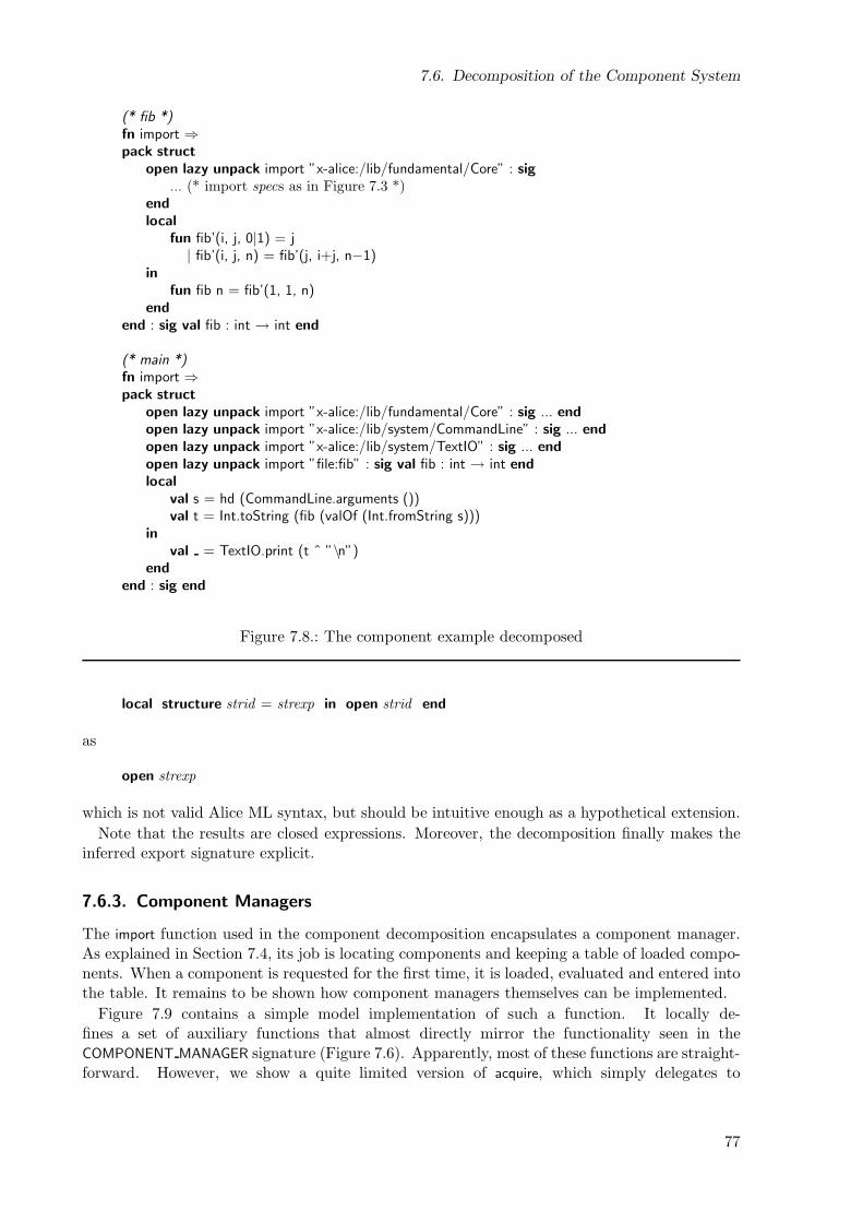
7.6. Decomposition of the Component System
(* fib *)fn import ⇒pack struct
open lazy unpack import ”x-alice:/lib/fundamental/Core” : sig
... (* import specs as in Figure 7.3 *)end
local
fun fib’(i, j, 0|1) = j| fib’(i, j, n) = fib’(j, i+j, n−1)
in
fun fib n = fib’(1, 1, n)end
end : sig val fib : int → int end
(* main *)fn import ⇒pack struct
open lazy unpack import ”x-alice:/lib/fundamental/Core” : sig ... end
open lazy unpack import ”x-alice:/lib/system/CommandLine” : sig ... end
open lazy unpack import ”x-alice:/lib/system/TextIO” : sig ... end
open lazy unpack import ”file:fib” : sig val fib : int → int end
local
val s = hd (CommandLine.arguments ())val t = Int.toString (fib (valOf (Int.fromString s)))
in
val = TextIO.print (t ˆ ”\n”)end
end : sig end
Figure 7.8.: The component example decomposed
local structure strid = strexp in open strid end
as
open strexp
which is not valid Alice ML syntax, but should be intuitive enough as a hypothetical extension.
Note that the results are closed expressions. Moreover, the decomposition finally makes theinferred export signature explicit.
7.6.3. Component Managers
The import function used in the component decomposition encapsulates a component manager.As explained in Section 7.4, its job is locating components and keeping a table of loaded compo-nents. When a component is requested for the first time, it is loaded, evaluated and entered intothe table. It remains to be shown how component managers themselves can be implemented.
Figure 7.9 contains a simple model implementation of such a function. It locally de-fines a set of auxiliary functions that almost directly mirror the functionality seen in theCOMPONENT MANAGER signature (Figure 7.6). Apparently, most of these functions are straight-forward. However, we show a quite limited version of acquire, which simply delegates to
77
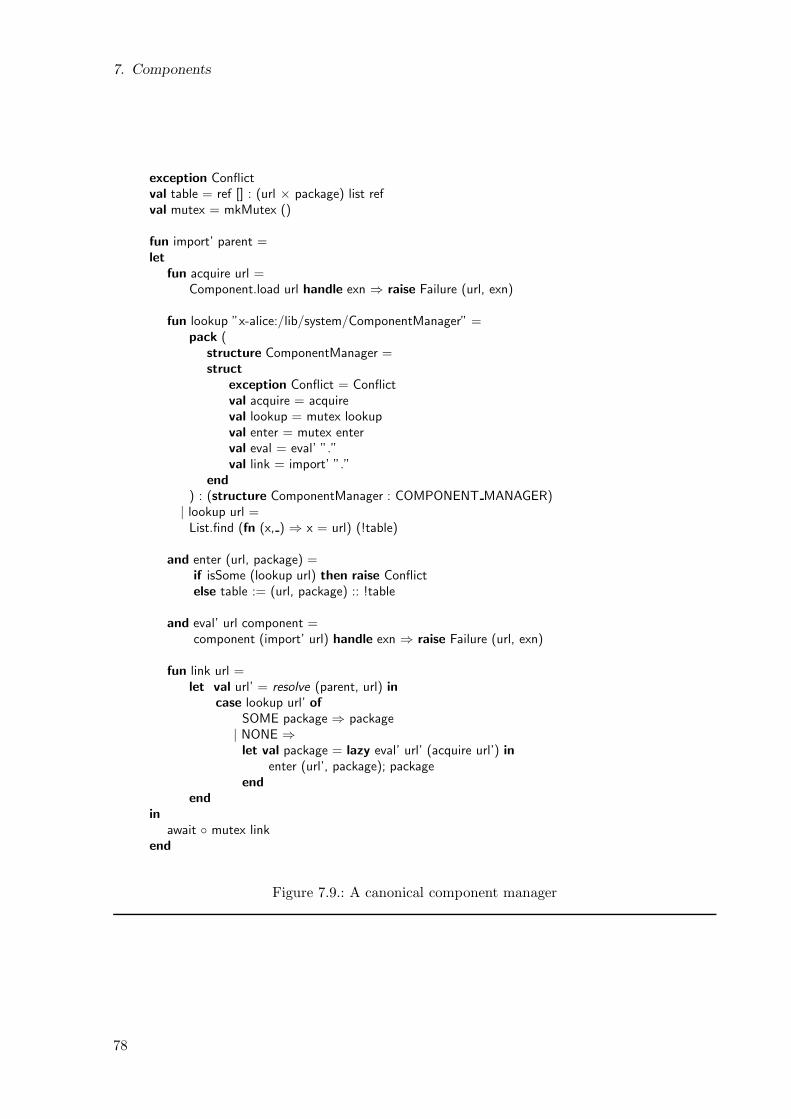
7. Components
exception Conflictval table = ref [] : (url × package) list refval mutex = mkMutex ()
fun import’ parent =let
fun acquire url =Component.load url handle exn ⇒ raise Failure (url, exn)
fun lookup ”x-alice:/lib/system/ComponentManager” =pack (
structure ComponentManager =struct
exception Conflict = Conflictval acquire = acquireval lookup = mutex lookupval enter = mutex enterval eval = eval’ ”.”val link = import’ ”.”
end
) : (structure ComponentManager : COMPONENT MANAGER)| lookup url =List.find (fn (x, ) ⇒ x = url) (!table)
and enter (url, package) =if isSome (lookup url) then raise Conflictelse table := (url, package) :: !table
and eval’ url component =component (import’ url) handle exn ⇒ raise Failure (url, exn)
fun link url =let val url’ = resolve (parent, url) in
case lookup url’ of
SOME package ⇒ package| NONE ⇒let val package = lazy eval’ url’ (acquire url’) in
enter (url’, package); packageend
end
in
await mutex linkend
Figure 7.9.: A canonical component manager
78
7.6. Decomposition of the Component System
Component.load (Section 7.2) and thus can only handle file URLs. For other URL schemes (par-ticularly http:) additional services may be accessed, which we will not describe here. We alsoignore primitive components.
The main complication is URL resolution: all URLs in an import declaration have to beinterpreted relative to the domain (authority) and path of the URL under which the importingcomponent was acquired. This is necessary to make groups of components relocatable acrossdirectory structures and network domains. Consequently, the import function passed to a com-ponent must know about the component’s associated URL, so that URL has to be passed as anadditional parent argument – import’ is the abstraction of import over this additional argument.Assuming existence of an auxiliary function resolve : url × url → url that syntactically resolvesa URL relative to another one, the internal link function can then perform the necessary reso-lution. When evaluating a component C, link passes along C’s URL to the evaluation functioneval’, which constructs an import function from it that is suitable for loading C’s own imports.
Explicit access to the component manager is enabled in this implementation by special-casingthe internal lookup function on the system URL of the component manager. If applied to thatURL, lookup just returns an appropriate package containing the required functionality. Note thatthese functions do not interpret URLs relative to a parent – no unambiguous notion of parentexists in their case, because the functions can be passed around first-class. Instead, URLs arepragmatically resolved relative to the local host and current working directory, which we indicatewith ”.” here.
The component table is stateful. To achieve thread safety, the manager must perform locking.We reuse the mutex abstraction from Section 6.5 for this purpose, which synchronises functionsvia mutual exclusion. All functions that access the table and are passed outside the closure –namely lookup, enter and link – are synchronised by applying the mutex.
Note that the link function enters the component into the table immediately, but actuallysuspends loading and evaluation through laziness. This is necessary to achieve re-entrancy ofthe manager, which is required because evaluating the component might spawn new threadsand request new components before returning. By returning from the synchronised link functionbefore actually initiating evaluation, the mutex lock is released first and a deadlock is avoided.To compensate, we must ensure that the lazy future is touched after the lock is released. We dothat by wrapping the synchronised link function with an explicit call to await to touch it.
7.6.4. Program Execution
Given the described reduction of components and component managers, execution of an AliceML program can be thought of as evaluation of the simple application
import’ ”.” root
where import’ refers to the initial component manager, and root is the URL of the program’s rootcomponent, resolved relative to the current host and working directory, which we again indicateby a dot URL.
In summary, all observable properties of program execution and dynamic linking follow fromthe decomposition we gave:
• Lazy Linking: Import is fully lazy. The first access to an imported component triggers itsactual loading, evaluation, and type checking.
• Type Propagation: Export signatures are dynamic types. Type checking fully takes dy-namic type equivalences into account. Through lazy types, a type check may triggerloading of other components.
79
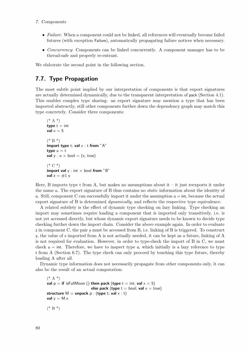
7. Components
• Failure: When a component could not be linked, all references will eventually become failedfutures (with exception Failure), automatically propagating failure notices when necessary.
• Concurrency: Components can be linked concurrently. A component manager has to bethread-safe and properly re-entrant.
We elaborate the second point in the following section.
7.7. Type Propagation
The most subtle point implied by our interpretation of components is that export signaturesare actually determined dynamically, due to the transparent interpretation of pack (Section 4.1).This enables complex type sharing: an export signature may mention a type that has beenimported abstractly, still other components further down the dependency graph may match thistype concretely. Consider three components:
(* A *)type t = intval x = 5
(* B *)import type t; val x : t from ”A”type u = tval y : u × bool = (x, true)
(* C *)import val y : int × bool from ”B”val z = #1 y
Here, B imports type t from A, but makes no assumptions about it – it just reexports it underthe name u. The export signature of B thus contains no static information about the identity ofu. Still, component C can successfully import it under the assumption u = int, because the actualexport signature of B is determined dynamically, and reflects the respective type equivalence.
A related subtlety is the effect of dynamic type checking on lazy linking. Type checking animport may sometimes require loading a component that is imported only transitively, i.e. isnot yet accessed directly, but whose dynamic export signature needs to be known to decide typechecking further down the import chain. Consider the above example again. In order to evaluatez in component C, the pair y must be accessed from B, i.e. linking of B is triggered. To constructy, the value of x imported from A is not actually needed, it can be kept as a future, linking of Ais not required for evaluation. However, in order to type-check the import of B in C, we mustcheck u = int. Therefore, we have to inspect type u, which initially is a lazy reference to typet from A (Section 6.7). The type check can only proceed by touching this type future, therebyloading A after all.
Dynamic type information does not necessarily propagate from other components only, it canalso be the result of an actual computation:
(* A *)val p = if isFullMoon () then pack (type t = int; val x = 5)
else pack (type t = bool; val x = true)structure M = unpack p : (type t; val x : t)val y = M.x
(* B *)
80
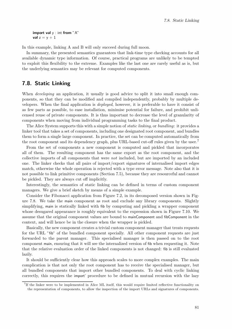
7.8. Static Linking
import val y : int from ”A”val z = y + 1
In this example, linking A and B will only succeed during full moon.
In summary, the presented semantics guarantees that link-time type checking accounts for allavailable dynamic type information. Of course, practical programs are unlikely to be temptedto exploit this flexibility to the extreme. Examples like the last one are rarely useful as is, butthe underlying semantics may be relevant for computed components.
7.8. Static Linking
When developing an application, it usually is good advice to split it into small enough com-ponents, so that they can be modified and compiled independently, probably by multiple de-velopers. When the final application is deployed, however, it is preferable to have it consist ofas few parts as possible, to ease installation, minimise potential for failure, and prohibit unli-censed reuse of private components. It is thus important to decrease the level of granularity ofcomponents when moving from individual programming tasks to the final product.
The Alice System supports this with a simple notion of static linking, or bundling : it provides alinker tool that takes a set of components, including one designated root component, and bundlesthem to form a single large component. In practice, the set can be computed automatically fromthe root component and its dependency graph, plus URL-based cut-off rules given by the user.7
From the set of components a new component is computed and pickled that incorporatesall of them. The resulting component has the same export as the root component, and thecollective imports of all components that were not included, but are imported by an includedone. The linker checks that all pairs of import/export signatures of internalised import edgesmatch, otherwise the whole operation is rejected with a type error message. Note also that it isnot possible to link primitive components (Section 7.5), because they are resourceful and cannotbe pickled. They are always cut off implicitly.
Interestingly, the semantics of static linking can be defined in terms of custom componentmanagers. We give a brief sketch by means of a simple example.
Consider the Fibonacci application from Figure 7.2, in its decomposed version shown in Fig-ure 7.8. We take the main component as root and exclude any library components. Slightlysimplifying, main is statically linked with fib by computing and pickling a wrapper componentwhose desugared appearance is roughly equivalent to the expression shown in Figure 7.10. Weassume that the original component values are bound to mainComponent and fibComponent in thecontext, and will hence be in the closure when the wrapper is pickled.
Basically, the new component creates a trivial custom component manager that treats requestsfor the URL ”fib” of the bundled component specially. All other component requests are justforwarded to the parent manager. This specialised manager is then passed on to the rootcomponent main, ensuring that it will see the internalized version of fib when requesting it. Notethat the relative evaluation order of the linked components is not changed: fib is still evaluatedlazily.
It should be sufficiently clear how this approach scales to more complex examples. The maincomplication is that not only the root component has to receive the specialised manager, butall bundled components that import other bundled components. To deal with cyclic linkingcorrectly, this requires the import’ procedure to be defined in mutual recursion with the lazy
7If the linker were to be implemented in Alice ML itself, this would require limited reflective functionality onthe representation of components, to allow the inspection of the import URLs and signatures of components.
81
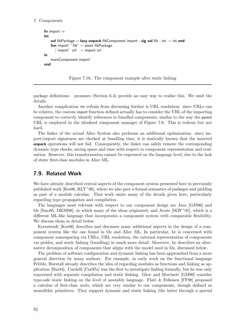
7. Components
fn import ⇒let
val fibPackage = lazy unpack fibComponent import : sig val fib : int → int end
fun import’ ”fib” = await fibPackage| import’ url = import url
in
mainComponent import’end
Figure 7.10.: The component example after static linking
package definitions – promises (Section 6.4) provide an easy way to realise this. We omit thedetails.
Another complication we refrain from discussing further is URL resolution: since URLs canbe relative, the custom import function defined actually has to consider the URL of the importingcomponent to correctly identify references to bundled components, similar to the way the parent
URL is employed in the idealised component manager of Figure 7.9. This is tedious but nothard.
The linker of the actual Alice System also performs an additional optimization: since im-port/export signatures are checked at bundling time, it is statically known that the insertedunpack operations will not fail. Consequently, the linker can safely remove the correspondingdynamic type checks, saving space and time with respect to component representation and eval-uation. However, this transformation cannot be expressed on the language level, due to the lackof static first-class modules in Alice ML.
7.9. Related Work
We have already described central aspects of the component system presented here in previouslypublished work [Ros06, RLT+06], where we also gave a formal semantics of packages and picklingas part of a module calculus. That work omits many of the details given here, particularlyregarding type propagation and compilation.
The languages most relevant with respect to our component design are Java [GJS96] andOz [Smo95, DKSS98], in which many of the ideas originated, and Acute [SLW+05], which is adifferent ML-like language that incorporates a component system with comparable flexibility.We discuss them in detail below.
Kornsteadt [Kor06] describes and discusses many additional aspects in the design of a com-ponent system like the one found in Oz and Alice ML. In particular, he is concerned withcomponent namespacing via URLs, URL resolution, the external representation of componentsvia pickles, and static linking (bundling) in much more detail. Moreover, he describes an alter-native decomposition of components that aligns with the model used in Oz, discussed below.
The problem of software configuration and dynamic linking has been approached from a moregeneral direction by many authors. For example, in early work on the functional languagePebble, Burstall already describes the idea of regarding modules as functions and linking as ap-plication [Bur84]. Cardelli [Car97a] was the first to investigate linking formally, but he was onlyconcerned with separate compilation and static linking. Glew and Morrisett [GM99] considertype-safe static linking on the level of assembly language. Flatt & Felleisen [FF98] proposeda calculus of first-class units, which are very similar to our components, though defined asmonolithic primitives. They support dynamic and static linking (the latter through a special
82
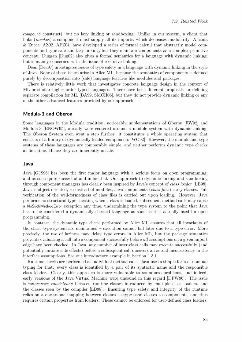
7.9. Related Work
compound construct), but no lazy linking or sandboxing. Unlike in our system, a client thatlinks (invokes) a component must supply all its imports, which decreases modularity. Ancona& Zucca [AZ02, AFZ04] have developed a series of formal calculi that abstractly model com-ponents and type-safe and lazy linking, but they maintain components as a complex primitiveconcept. Duggan [Dug02] also gives a formal semantics for a language with dynamic linking,but is mainly concerned with the issue of recursive linking.
Dean [Dea97] investigates issues of type safety in a language with dynamic linking in the styleof Java. None of these issues arise in Alice ML, because the semantics of components is definedpurely by decomposition into (safe) language features like modules and packages.
There is relatively little work that investigates concrete language design in the context ofML or similar higher-order typed languages. There have been different proposals for definingseparate compilation for ML [BA99, SMCH06], but they do not provide dynamic linking or anyof the other advanced features provided by our approach.
Modula-3 and Oberon
Some languages in the Modula tradition, noticeably implementations of Oberon [RW92] andModula-3 [BNOW95], already were centered around a module system with dynamic linking.The Oberon System even went a step further: it constitutes a whole operating system thatconsists of a library of dynamically loaded components [WG92]. However, the module and typesystems of these languages are comparably simple, and neither performs dynamic type checksat link time. Hence they are inherently unsafe.
Java
Java [GJS96] has been the first major language with a serious focus on open programming,and as such quite successful and influential. Our approach to dynamic linking and sandboxingthrough component managers has clearly been inspired by Java’s concept of class loader [LB98].Java is object-oriented, so instead of modules, Java components (class files) carry classes. Fullverification of the well-formedness of class files is carried out upon loading. However, Javaperforms no structural type checking when a class is loaded, subsequent method calls may causea NoSuchMethodError exception any time, undermining the type system to the point that Javahas to be considered a dynamically checked language as soon as it is actually used for openprogramming.
In contrast, the dynamic type check performed by Alice ML ensures that all invariants ofthe static type system are maintained – execution cannot fail later due to a type error. Moreprecisely, the use of laziness may delay type errors in Alice ML, but the package semanticsprevents evaluating a call into a component successfully before all assumptions on a given importedge have been checked. In Java, any number of inter-class calls may execute successfully (andpotentially initiate side effects) before a subsequent call uncovers an actual inconsistency in theinterface assumptions. See our introductory example in Section 1.3.1.
Runtime checks are performed at individual method calls. Java uses a simple form of nominaltyping for that: every class is identified by a pair of its syntactic name and the responsibleclass loader. Clearly, this approach is more vulnerable to soundness problems, and indeed,early versions of the Java Virtual Machine were unsound in this regard [DFW96]. The issueis namespace consistency between runtime classes introduced by multiple class loaders, andthe classes seen by the compiler [LB98]. Ensuring type safety and integrity of the runtimerelies on a one-to-one mapping between classes as types and classes as components, and thusrequires certain properties from loaders. These cannot be enforced for user-defined class loaders.
83
7. Components
Consequently, the Java runtime not only has to ensure that no class loader is ever invoked twicefor the same class, it also has to double-check the name of classes delivered by a loader.
None of these problems exist in Alice ML, where type identity is established by generativity,and type safety thus is completely independent from the identity of components. Consequently,component managers are safe by construction, since they can be expressed solely in terms ofproper language constructs, which are known to be type-safe. Even nonsensical managers, e.g.ones that deliver a different component each time the same URL is requested, cannot compromisesoundness.
Java has a built-in mechanism for serialization that even supports versioning. However, it isnot interchangeable with class files and not generic. In particular, code cannot be serialised, onlyclass names can be used to represent code in serialised objects, which is a comparatively inflexibleand fragile abstraction. Consequently, there is no equivalent to computed components. Instead,if required, classes have to be exchanged manually as class files, separate from objects. In thecase of distributed programming, the Java RMI (remote method invocation) framework [WRW96]encapsulates transmission of class files in the library. Classes can be loaded as first-class entities,but as such they can only be accessed indirectly per Java’s reflection mechanism, which precludesany form of static type checking.
Java was originally intended for writing applets running in Web browsers. For that purpose,Java provides sandboxing as an integral part of its runtime infrastructure. Custom class loadersallow to control access to certain classes. Every class loader is accompanied by a security managerthat checks access on a per-operation basis. In more recent versions, the sandbox model hasbeen refined with a system of cryptographically verified trust and more fine-grained, user-definedpermissions and policies. The sandboxing infrastructure needs to be built into the core systemin Java, in contrast to our approach, where it can be realised fully within the language.
Java Archives (JARs) are bundled collections of Java class files. Unlike static linking in AliceML, creation of Java archives does not perform type checks, and intra-archive linking can stillfail at runtime.
Scala
Scala [Ode05] is a hybrid object-oriented/functional language on top of the Java infrastructure.It has a very powerful static type and class system [OCRZ03] that subsumes Java as well asmuch of ML modules, and additionally provides features like multiple inheritance, mixins, andviews.
Still, open programming in Scala suffers from the same shortcomings as in Java, due to itsapproach of reusing most of Java’s runtime and library. It hence inherits most of Java’s problemsregarding open programming. In particular, the expressiveness of the static type system does notcarry over to dynamic typing, because Scala types are erased to Java types during compilation.
“.NET”
The Microsoft “.NET” Common Language Runtime [Mic03] is a framework that is very similarto the Java Virtual Machine and library in most aspects related to open programming, butis meant to support multiple languages. Unlike Java it allows components (assemblies) to becreated dynamically via its reflection mechanism, but like Java class files, assemblies can onlycontain static data of very limited form.
84
7.9. Related Work
Oz
The overall design of the component system for Alice ML was directly inspired by Oz [Smo95,VH04], which also has a first-class component system with lazy linking, computed components,managers, and a definition by decomposition [DKSS98, Kor06]. Dynamic linking in Oz in turnwas partially inspired by Java’s class loading mechanism.
Oz components are called functors. Like our components, they depend on a number of importsidentified by URLs, and provide a record of values as export. Linking is performed by a modulemanager, which directly corresponds to our component manager. Functors are represented aspickles externally, although these are not interchangeable with plain pickles like in our design(all functor files are pickles, but not vice versa). As an extension to the system presented here,Oz provides syntactic sugar for creating computed components directly during compilation.
With Oz being an untyped language, no dynamic type-checking is performed for imports.The decomposition of Oz components thus differs from the one in our approach (Section 7.6):instead of being abstracted over an indirect linking function, Oz functors are directly representedas functions over the tuple of import modules. This approach is inapplicable in a typed setting,because there would be no fixed representation type for components: import signatures aredependently typed, which precludes passing imports as homogeneous variable-length vectors– thus component functions would actually have to vary in arity. Linking in the Oz modelrequires reflective capabilities that cannot be typed either. Moreover, the model cannot capturethe actual type-checking semantics, especially the fact that export signatures are dynamicallycomputed by evaluating the component. Consequently, the interplay between dynamic type-checking and lazy types could not be reflected properly either.
Another difference between the two approaches is that Oz makes the linking policy [Kor06](e.g. use of laziness) the responsibility of the manager, while our approach could allow everycomponent to select it on a per-import basis. This has the arguable advantage that it rendersthe semantics of imports more transparent and the manager itself becomes somewhat simpler.Another advantage we see in our approach is that imports are clearly modelled as implementationdetails of a component, which mirrors the language-level situation more accurately.8
Acute
Acute [SLW+05] is an experimental, ML-like language for typed open programming, probablyclosest in spirit to Alice ML. It addresses many issues of open programming, including type-safe pickling (marshalling), abstraction safety, dynamic linking, and even versioning [Sew01,BHS+03].
Although Acute has no explicit notion of component, modules can be lazily imported fromfiles or URLs very much like in Alice ML. The module system itself is simple: only structuresare supported, functors are not available.
Instead of providing first-class or computed components, pickling in Acute incorporates adifferent mechanism for controlling rebinding: individual modules can be declared as “imported”,which means that they are potentially rebound on the target site when the pickle is loaded. Theprecise extent of rebinding is controlled by decorating a program with symbolic marks. A picklingoperation can then initiate rebinding up to a particular mark. This approach crucially requiresprograms to be viewed as linear sequences of module definitions. To control rebinding properly,a programmer might have to construct a program such that a suitable global ordering on allits modules and marks is imposed. Hence the approach appears to be inherently unmodular;
8Only static linking requires knowledge about the import list, at least if computation of the dependency graphshould be automatic.
85
7. Components
it is not clear how the ordering could be maintained in the presence independently developedlibraries, which might even have conflicting requirements on imports shared in a diamond-graphmanner.
In contrast, Alice ML’s computed components allow rebinding to be controlled locally andmuch more fine-grained. On the other hand, they do not enable rebinding in pre-computedparts of the component – i.e. abstraction after the fact. That is possible with Acute’s markmechanism, although even marks cover only a limited class of cases. For example, there seemsto be no way to control rebinding of modules that do not appear in the static program text, butwere implicitly received by a preceding unmarshalling operation.
Acute takes a more monolithic approach to language design: its mechanisms are all built-inas comparatively complex language constructs, with no obvious reduction into simpler conceptslike in our approach. For example, there is no equivalent to component managers, the completelinking process is primitive in the language semantics.
A severe consequence is that linking strategies cannot be customised by the programmer. Dueto that – and Acute’s uncontrolled implicit rebinding – it is not clear how sandboxing or othersecurity mechanism could be programmed. Static linking can be simulated to a limited extendusing Acute’s inclusion mechanism for compiled code.
Acute provides a number of interesting features not available in Alice ML. Most notably,module definitions and imports can be decorated with versioning constraints, which are checkedduring linking. Moreover, Acute gives means to redefine the implementation of existing modules,by explicitly breaking type abstractions in a type-safe manner (i.e. without changing the actualrepresentation of abstract types). The latter violates abstraction safety, but Sewell et al. arguethat it is necessary to support software evolution in practice [SLW+05].
7.10. Summary
• Alice ML recasts the component system from Oz in a typed context.
• Components complement ML’s static module system with type-safe, lazy dynamic linking.
• Alice ML is unique in that components are strongly typed by dynamic higher-order modulesignatures.
• Through structural signature subtyping, link-time type checking is robust against interfacechanges.
• Every source file is interpreted as a component definition with an implicit signature.
• Components can also be computed dynamically, and thus allow processes to exchangebehaviour that encapsulates dynamic information and depends on local resources.
• Customisable component managers give control over imports and enable security policiesfor resources.
• Static bundling allows formation of large components from smaller ones.
• The component system can be explained solely in terms of modules, packages and futures.The model differs from previous work in that export signatures are computed from concretedynamic type information.
86
8. Distribution
Networks are ubiquitous in today’s computing world. Fast local networks connect individualmachines and enable them to share resources, either in hardware or software. Slower globalnetworks – particularly the Internet – connect computers and local networks all over the worldand enable them to communicate and exchange various kinds of data.
Many applications today are distributed over multiple communicating and cooperating ma-chines:
• Classical client/server applications, where multiple client programs benefit from servicesprovided by a (single) server program. The most dominant example of this architecturetoday is the World Wide Web.
• Peer-to-peer applications, where many programs connect to each other and form a dynamicnetwork for storing, locating and exchanging information. File sharing software is a popularexample.
• Cluster and grid computing, where a large number of machines shares computational re-sources to solve costly tasks in parallel. For example, this concept is found in renderfarms creating computer-generated imagery (CGI), or search engines indexing large setsof data [DG04].
• Mobile agents, where autonomous programs migrate between different sites to gather in-formation, manage a network, deploy software, or perform other tasks. Ironically, the mostwide-spread incarnation of this principle today are computer viruses.
A lot can be said about distributed programming, its applications, techniques, and the problemsinvolved. However, within the scope of this thesis, we are mainly concerned with the problemof establishing type safety across process boundaries. We deliberately stay ignorant aboutother delicate aspects of distributed programming – like network latency, failure recovery, etc.Excellent work exists in literature that covers these issues, one good starting point is the thesisof Armstrong [Arm03]. The rest of this chapter restricts itself to describing the basic languageprimitives that exist in Alice ML to support distributed programming, along with a few simpleexamples that illuminate questions of typing.
A distributed system consists of a number of interacting processes. Every process executes aprogram. The processes run on potentially different sites in a network. We will use the termsprocess and site almost interchangeably, to emphasise that processes are usually located onphysically different locations in a network.
The goal of having language support for distribution is to allow processes to be expressed ashigh-level Alice ML programs. The design we present offers the following desirable properties:
• Network transparency. A process can obtain references to values in another process(remote values), which are handled in (almost) the same way as local values. Hence thesame abstraction mechanisms and idioms can be applied for local and remote operationsand communication.
87
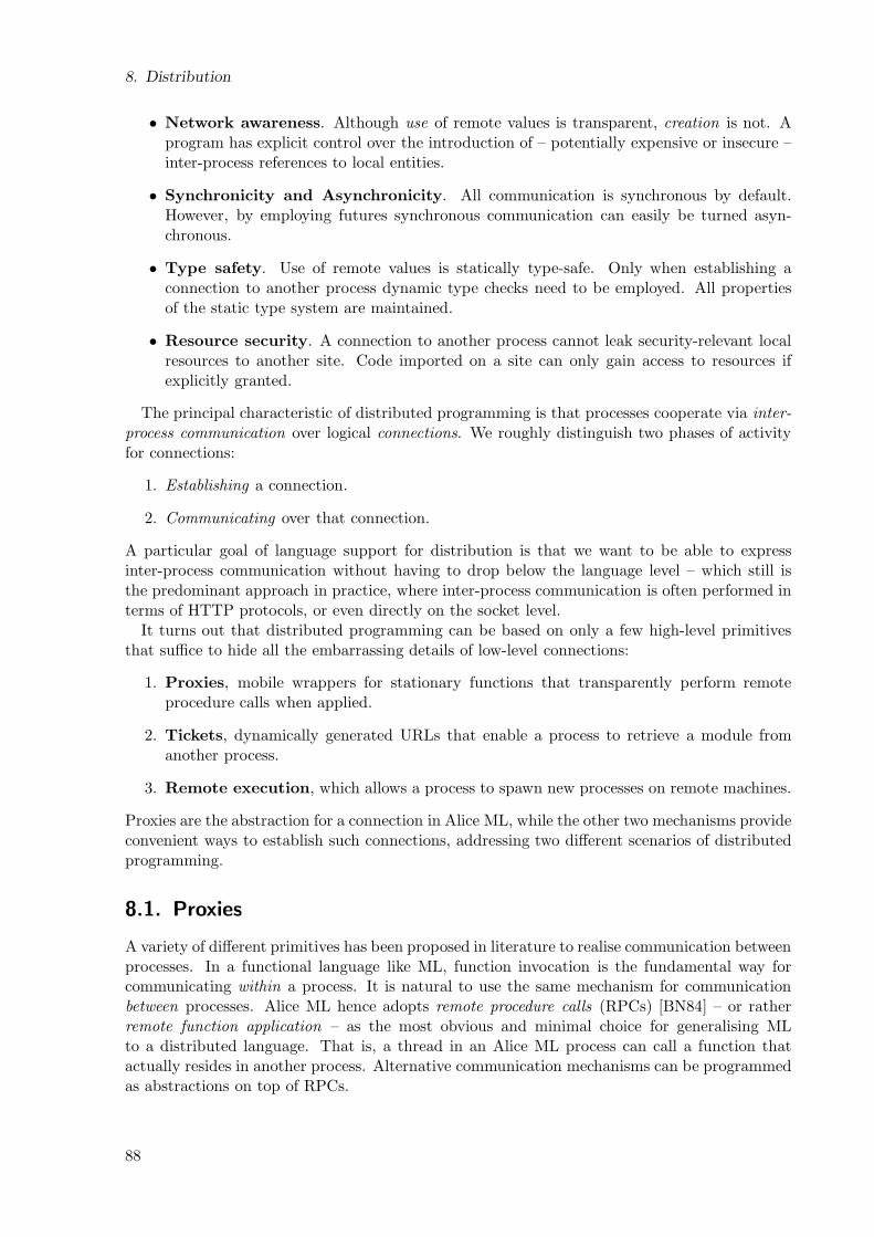
8. Distribution
• Network awareness. Although use of remote values is transparent, creation is not. Aprogram has explicit control over the introduction of – potentially expensive or insecure –inter-process references to local entities.
• Synchronicity and Asynchronicity. All communication is synchronous by default.However, by employing futures synchronous communication can easily be turned asyn-chronous.
• Type safety. Use of remote values is statically type-safe. Only when establishing aconnection to another process dynamic type checks need to be employed. All propertiesof the static type system are maintained.
• Resource security. A connection to another process cannot leak security-relevant localresources to another site. Code imported on a site can only gain access to resources ifexplicitly granted.
The principal characteristic of distributed programming is that processes cooperate via inter-process communication over logical connections. We roughly distinguish two phases of activityfor connections:
1. Establishing a connection.
2. Communicating over that connection.
A particular goal of language support for distribution is that we want to be able to expressinter-process communication without having to drop below the language level – which still isthe predominant approach in practice, where inter-process communication is often performed interms of HTTP protocols, or even directly on the socket level.
It turns out that distributed programming can be based on only a few high-level primitivesthat suffice to hide all the embarrassing details of low-level connections:
1. Proxies, mobile wrappers for stationary functions that transparently perform remoteprocedure calls when applied.
2. Tickets, dynamically generated URLs that enable a process to retrieve a module fromanother process.
3. Remote execution, which allows a process to spawn new processes on remote machines.
Proxies are the abstraction for a connection in Alice ML, while the other two mechanisms provideconvenient ways to establish such connections, addressing two different scenarios of distributedprogramming.
8.1. Proxies
A variety of different primitives has been proposed in literature to realise communication betweenprocesses. In a functional language like ML, function invocation is the fundamental way forcommunicating within a process. It is natural to use the same mechanism for communicationbetween processes. Alice ML hence adopts remote procedure calls (RPCs) [BN84] – or ratherremote function application – as the most obvious and minimal choice for generalising MLto a distributed language. That is, a thread in an Alice ML process can call a function thatactually resides in another process. Alternative communication mechanisms can be programmedas abstractions on top of RPCs.
88
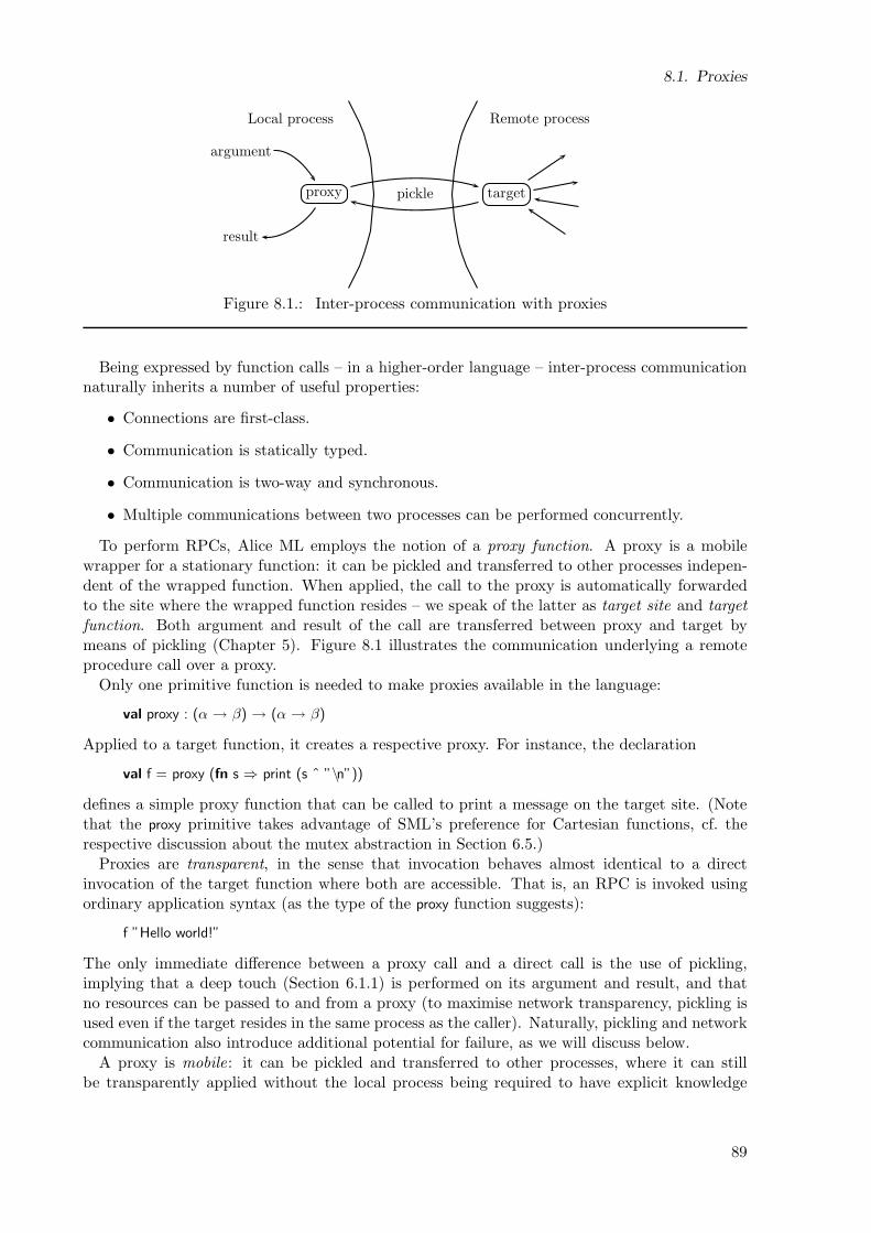
8.1. Proxies
argument
result
proxy targetpickle
Local process Remote process
Figure 8.1.: Inter-process communication with proxies
Being expressed by function calls – in a higher-order language – inter-process communicationnaturally inherits a number of useful properties:
• Connections are first-class.
• Communication is statically typed.
• Communication is two-way and synchronous.
• Multiple communications between two processes can be performed concurrently.
To perform RPCs, Alice ML employs the notion of a proxy function. A proxy is a mobilewrapper for a stationary function: it can be pickled and transferred to other processes indepen-dent of the wrapped function. When applied, the call to the proxy is automatically forwardedto the site where the wrapped function resides – we speak of the latter as target site and targetfunction. Both argument and result of the call are transferred between proxy and target bymeans of pickling (Chapter 5). Figure 8.1 illustrates the communication underlying a remoteprocedure call over a proxy.
Only one primitive function is needed to make proxies available in the language:
val proxy : (α → β) → (α → β)
Applied to a target function, it creates a respective proxy. For instance, the declaration
val f = proxy (fn s ⇒ print (s ˆ ”\n”))
defines a simple proxy function that can be called to print a message on the target site. (Notethat the proxy primitive takes advantage of SML’s preference for Cartesian functions, cf. therespective discussion about the mutex abstraction in Section 6.5.)
Proxies are transparent, in the sense that invocation behaves almost identical to a directinvocation of the target function where both are accessible. That is, an RPC is invoked usingordinary application syntax (as the type of the proxy function suggests):
f ”Hello world!”
The only immediate difference between a proxy call and a direct call is the use of pickling,implying that a deep touch (Section 6.1.1) is performed on its argument and result, and thatno resources can be passed to and from a proxy (to maximise network transparency, pickling isused even if the target resides in the same process as the caller). Naturally, pickling and networkcommunication also introduce additional potential for failure, as we will discuss below.
A proxy is mobile: it can be pickled and transferred to other processes, where it can stillbe transparently applied without the local process being required to have explicit knowledge
89

8. Distribution
of the originating site – this knowledge is encapsulated in the proxy. The important featurehere is that, when pickling a proxy, the target function is not pickled along with it – contrastthis to pickling of ordinary functions that have other functions in their closure (Section 5.1).In particular, the target function can be sited (Section 5.3) without compromising mobility ofthe proxy. This is the only deviation that Alice ML makes from the closedness principle forpickles (Section 5.1) – it is crucial however to allow capturing connections to processes in pickles(because obviously, processes cannot be included in a pickle).
A connection to another process now simply consists of a proxy that has been created in thatprocess. Receiving a proxy can be understood as establishing a connection. Communication isengaged by calling a proxy. For instance, if we pickle the above proxy function to a file,
Pickle.save (”/home/rossberg/hello”, pack (val it = f) : (val it : string → unit))
and load the pickle in a second process (that has access to the same file system) then we cansend a greeting to the first process:
structure H = unpack Pickle.load ”/home/rossberg/hello” : (val it : string → unit)H.it ”Hello world!”
Note that we could not have pickled the target function itself, because print is a sited operation!Proxies are typed connections. A proxy invocation is statically type-safe because proxies can
only be received through pickles, where type consistency is always ensured. In other words,once the connection is established – by successfully receiving the proxy – no further type checksare required. However, the runtime system may need to perform verification (Section 5.2) ofarguments or results received for proxy calls, if it does not trust the other process (Section 8.4).
All invocations of a proxy are synchronous: the call to H.it in the above example does notreturn before the message has been printed in the remote process. However, asynchronous callscan easily be achieved by employing futures (Section 6.1.2):
spawn H.it ”Hello world!”
Now we have turned the application into an asynchronous remote call – it immediately evaluatesto a future. In other words, futures give us the ability to use just one uniform RPC semanticswhile still providing synchronous and asynchronous calls, orthogonally. More interestingly, un-like asynchronous calls in most other languages, futures in Alice ML enable even asynchronouscalls to return results. This feature allows to conveniently formulate bi-directional query/replycommunication while still hiding network latency as much as possible.
The function proxy is provided in the structure Remote of the Alice library, whose signature isshown in Figure 8.2. Besides other functions explained in the following sections, it also containsa higher-order polymorphic functor Proxy, which conveniently allows wrapping all functions in agiven structure (or functor) into proxies in one go. For example, we can give another Alice MLprocess access to local I/O by wrapping the whole TextIO structure and pickling the result:
Pickle.save (”myio”, pack Proxy (signature S=TEXT IO; structure X=TextIO) : TEXT IO)
The Proxy functor uses the dynamic signature information to operate in a type-directed manner.Consequently, it is able to handle even curried functions correctly, by recursively wrapping eachpartial application in its own proxy. For example,
Proxy (signature S = sig val f : string → string → string end
structure X = struct fun f s1 = (print s1; fn s2 ⇒ (print s2; s1ˆs2)) end)
returns a structure containing a wrapper for f as follows:
proxy (fn s1 ⇒ proxy (f s1))
90
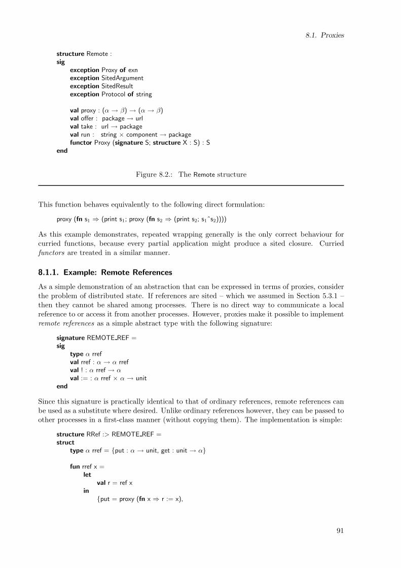
8.1. Proxies
structure Remote :sig
exception Proxy of exnexception SitedArgumentexception SitedResultexception Protocol of string
val proxy : (α → β) → (α → β)val offer : package → urlval take : url → packageval run : string × component → packagefunctor Proxy (signature S; structure X : S) : S
end
Figure 8.2.: The Remote structure
This function behaves equivalently to the following direct formulation:
proxy (fn s1 ⇒ (print s1; proxy (fn s2 ⇒ (print s2; s1ˆs2))))
As this example demonstrates, repeated wrapping generally is the only correct behaviour forcurried functions, because every partial application might produce a sited closure. Curriedfunctors are treated in a similar manner.
8.1.1. Example: Remote References
As a simple demonstration of an abstraction that can be expressed in terms of proxies, considerthe problem of distributed state. If references are sited – which we assumed in Section 5.3.1 –then they cannot be shared among processes. There is no direct way to communicate a localreference to or access it from another processes. However, proxies make it possible to implementremote references as a simple abstract type with the following signature:
signature REMOTE REF =sig
type α rrefval rref : α → α rrefval ! : α rref → αval := : α rref × α → unit
end
Since this signature is practically identical to that of ordinary references, remote references canbe used as a substitute where desired. Unlike ordinary references however, they can be passed toother processes in a first-class manner (without copying them). The implementation is simple:
structure RRef :> REMOTE REF =struct
type α rref = put : α → unit, get : unit → α
fun rref x =let
val r = ref xin
put = proxy (fn x ⇒ r := x),
91
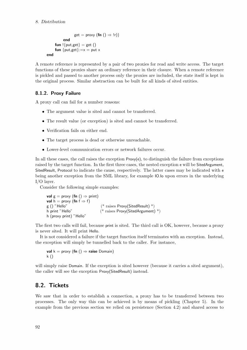
8. Distribution
get = proxy (fn () ⇒ !r)end
fun !put,get = get ()fun put,get:=x = put x
end
A remote reference is represented by a pair of two proxies for read and write access. The targetfunctions of these proxies share an ordinary reference in their closure. When a remote referenceis pickled and passed to another process only the proxies are included, the state itself is kept inthe original process. Similar abstraction can be built for all kinds of sited entities.
8.1.2. Proxy Failure
A proxy call can fail for a number reasons:
• The argument value is sited and cannot be transferred.
• The result value (or exception) is sited and cannot be transferred.
• Verification fails on either end.
• The target process is dead or otherwise unreachable.
• Lower-level communication errors or network failures occur.
In all these cases, the call raises the exception Proxy(e), to distinguish the failure from exceptionsraised by the target function. In the first three cases, the nested exception e will be SitedArgument,SitedResult, Protocol to indicate the cause, respectively. The latter cases may be indicated with e
being another exception from the SML library, for example IO.Io upon errors in the underlyingI/O layer.
Consider the following simple examples:
val g = proxy (fn () ⇒ print)val h = proxy (fn f ⇒ f)g () ”Hello” (* raises Proxy(SitedResult) *)h print ”Hello” (* raises Proxy(SitedArgument) *)h (proxy print) ”Hello”
The first two calls will fail, because print is sited. The third call is OK, however, because a proxyis never sited. It will print Hello.
It is not considered a failure if the target function itself terminates with an exception. Instead,the exception will simply be tunnelled back to the caller. For instance,
val k = proxy (fn () ⇒ raise Domain)k ()
will simply raise Domain. If the exception is sited however (because it carries a sited argument),the caller will see the exception Proxy(SitedResult) instead.
8.2. Tickets
We saw that in order to establish a connection, a proxy has to be transferred between twoprocesses. The only way this can be achieved is by means of pickling (Chapter 5). In theexample from the previous section we relied on persistence (Section 4.2) and shared access to
92
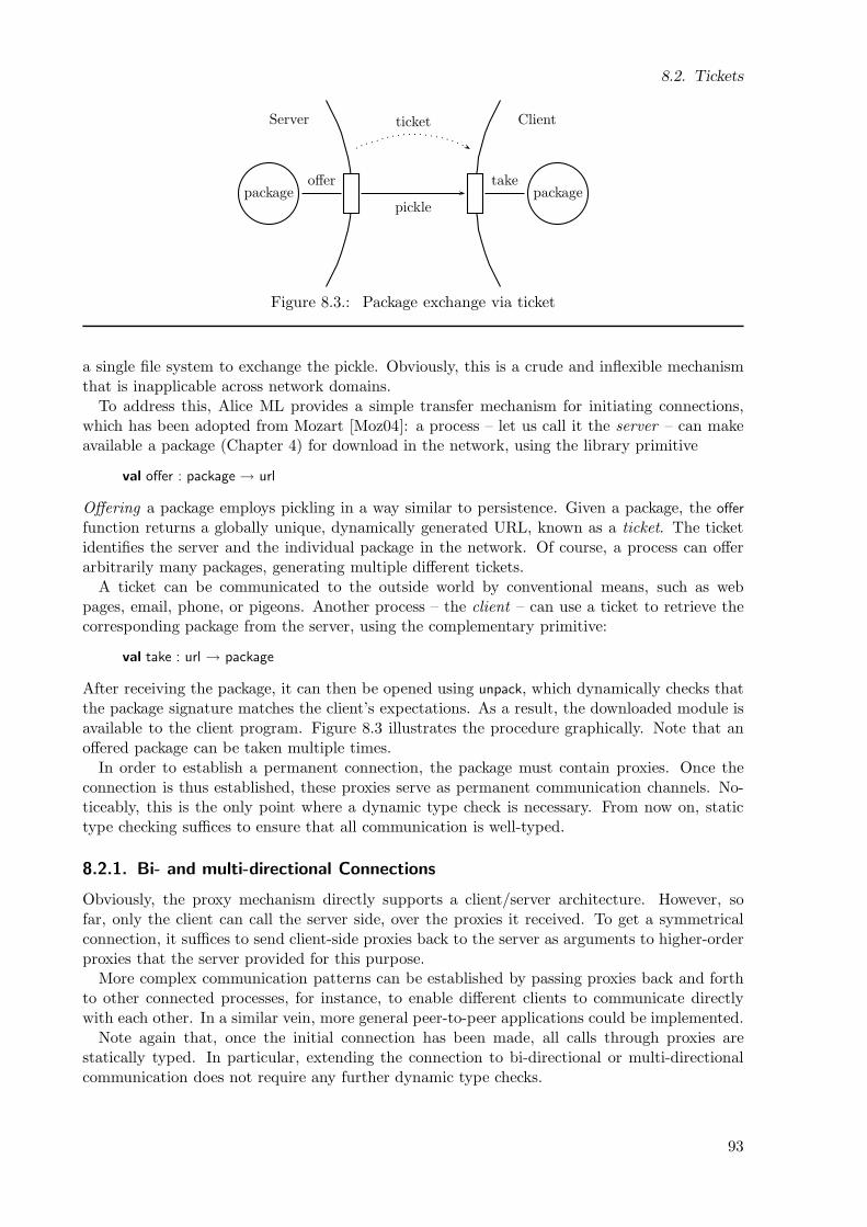
8.2. Tickets
package packageoffer
pickle
take
ticketServer Client
Figure 8.3.: Package exchange via ticket
a single file system to exchange the pickle. Obviously, this is a crude and inflexible mechanismthat is inapplicable across network domains.
To address this, Alice ML provides a simple transfer mechanism for initiating connections,which has been adopted from Mozart [Moz04]: a process – let us call it the server – can makeavailable a package (Chapter 4) for download in the network, using the library primitive
val offer : package → url
Offering a package employs pickling in a way similar to persistence. Given a package, the offer
function returns a globally unique, dynamically generated URL, known as a ticket. The ticketidentifies the server and the individual package in the network. Of course, a process can offerarbitrarily many packages, generating multiple different tickets.
A ticket can be communicated to the outside world by conventional means, such as webpages, email, phone, or pigeons. Another process – the client – can use a ticket to retrieve thecorresponding package from the server, using the complementary primitive:
val take : url → package
After receiving the package, it can then be opened using unpack, which dynamically checks thatthe package signature matches the client’s expectations. As a result, the downloaded module isavailable to the client program. Figure 8.3 illustrates the procedure graphically. Note that anoffered package can be taken multiple times.
In order to establish a permanent connection, the package must contain proxies. Once theconnection is thus established, these proxies serve as permanent communication channels. No-ticeably, this is the only point where a dynamic type check is necessary. From now on, statictype checking suffices to ensure that all communication is well-typed.
8.2.1. Bi- and multi-directional Connections
Obviously, the proxy mechanism directly supports a client/server architecture. However, sofar, only the client can call the server side, over the proxies it received. To get a symmetricalconnection, it suffices to send client-side proxies back to the server as arguments to higher-orderproxies that the server provided for this purpose.
More complex communication patterns can be established by passing proxies back and forthto other connected processes, for instance, to enable different clients to communicate directlywith each other. In a similar vein, more general peer-to-peer applications could be implemented.
Note again that, once the initial connection has been made, all calls through proxies arestatically typed. In particular, extending the connection to bi-directional or multi-directionalcommunication does not require any further dynamic type checks.
93
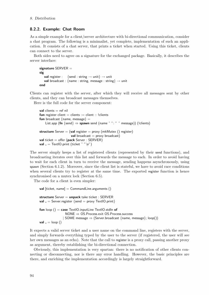
8. Distribution
8.2.2. Example: Chat Room
As a simple example for a client/server architecture with bi-directional communication, considera chat program. The following is a minimalist, yet complete, implementation of such an appli-cation. It consists of a chat server, that prints a ticket when started. Using this ticket, clientscan connect to the server.
Both sides need to agree on a signature for the exchanged package. Basically, it describes theserver interface:
signature SERVER =sig
val register : send : string → unit → unitval broadcast : name : string, message : string → unit
end
Clients can register with the server, after which they will receive all messages sent by otherclients, and they can broadcast messages themselves.
Here is the full code for the server component:
val clients = ref nilfun register client = clients := client :: !clientsfun broadcast name, message =
List.app (fn send ⇒ spawn send (name ˆ ”: ” ˆ message)) (!clients)
structure Server = (val register = proxy (mkMutex () register)val broadcast = proxy broadcast)
val ticket = offer (pack Server : SERVER)val = TextIO.print (ticket ˆ ”\n”)
The server simply keeps a list of registered clients (represented by their send functions), andbroadcasting iterates over this list and forwards the message to each. In order to avoid havingto wait for each client in turn to receive the message, sending happens asynchronously, usingspawn (Section 6.1.2). Moreover, since the client list is stateful, we have to avoid race conditionswhen several clients try to register at the same time. The exported register function is hencesynchronised on a mutex lock (Section 6.5).
The code for a client is even simpler:
val [ticket, name] = CommandLine.arguments ()
structure Server = unpack take ticket : SERVERval = Server.register send = proxy TextIO.print
fun loop () = case TextIO.inputLine TextIO.stdIn of
NONE ⇒ OS.Process.exit OS.Process.success| SOME message ⇒ (Server.broadcast name, message; loop())
val = loop ()
It expects a valid server ticket and a user name on the command line, registers with the server,and simply forwards everything typed by the user to the server (if registered, the user will seeher own messages as an echo). Note that the call to register is a proxy call, passing another proxyas argument, thereby establishing the bi-directional connection.
Obviously, this implementation is very spartan: there is no notification of other clients con-necting or disconnecting, nor is there any error handling. However, the basic principles arethere, and enriching the implementation accordingly is largely straightforward.
94
8.3. Remote Execution
With respect to multi-directional connections, the client/server interface could be extendedsuch that the server can hand send functions from one client to another. The latter client couldthen send private messages to the former itself, directly, without further assistance from theserver.
8.3. Remote Execution
In the client/server setting, client processes choose independently to connect to a known serverprocess. A different scenario of distributed programming arises in applications like cluster com-puting. There, we usually find a master process (sometimes known as the manager) that shiftscomputational tasks to a number of slaves (or workers). In this scenario, it is the central masterwho initiates connections, by actually spawning new processes on remote machines.
To support this scenario, the Remote module of the Alice ML library features a further function:
val run : string × component → package
This function performs most of the required procedure: it connects to a remote machine byusing a low-level service (such as ssh), the host name is given by the string argument. On thatmachine it starts a fresh Alice ML process as slave. The slave immediately connects to themaster to receive the component argument, and evaluates the component. It sends back theresulting module as a package.
The transmitted component will typically be computed (Section 7.2) in the master process.By capturing proxies defined outside of the component, and by creating proxies inside it andexporting them, a two-way communication is immediately established.
8.3.1. Example: Distributed Search
Let us illustrate remote execution – and other features of Alice ML – by showing the imple-mentation of a distributed application, namely a distributed solver for constraint program-ming [Apt03, Sch02]. This example is taken from [RLT+06].
In the context of constraint programming, a solver is a program that explores a search treein order to find the solutions of a given constraint problem. Nodes of the tree represent choicepoints, leaves represent either solutions or failures (where previous choices are inconsistent).From a logical point of view, searching amounts to traversing a tree and asking the status ofeach leaf node.
In a distributed setting, a number of workers perform the search, such that each worker ex-plores a different subtree. The interesting information, that is the solutions, are transmittedback to a manager. The manager also organises the search. In the following, we focus on thedistribution aspect. Details about the search itself can be found in [TL04], which contains aformalisation of the underlying abstractions, performing efficient backtracking and vital optimi-sations such as branch and bound.
The interface between the workers and the manager can be represented as shown in Fig-ure 8.4 [Sch02]:
• find is sent by an idle worker to request a new job, that is, the path of a subtree thatremains to be explored.
• collect is send by a worker when it finds a solution. The message will contain the respectivesolution.
95
8. Distribution
manager worker
share
explore
stop
find
collect
Figure 8.4.: Distributed search interface
• share is used by the manager to ask a worker whether it can give away a subtree thatremains to be explored. The worker is required to answer either negatively, or positivelyby providing the path associated with the corresponding unexplored subtree.
• explore commands a worker to explore the subtree at a given path.
• stop is used to interrupt a worker when the search is finished.
The implementation of the distributed search engine consists of two components: the managerand the worker. The manager creates workers by using the Remote.run primitive. Each workerhas the same interface:
signature WORKER =sig
val share : unit → path optionval explore : path → unitval stop : unit → unit
end
Workers are components dynamically computed by the manager (Section 7.2). They captureproxies to the two functions find and collect of the manager interface in their closure. The managerhence defines these functions as follows:
val find = proxy (fn () ⇒ (* request new subtree from a worker and return its path *))val collect = proxy (fn sol ⇒ (* store sol; request new subtree and explore *))
Since a worker is a computed component, the definition of a worker also takes place in themanager. Basically, we create a computed component that exports the three operations share,explore, and stop from the WORKER signature. Naturally, they are also defined as proxies. Butsince the component is evaluated on the remote site, the proxies are created there and thusrepresent an inverse connection:
val worker =comp
import structure Gecode from ”x-alice:/lib/Gecode”with
include WORKERin
val share = proxy (fn () ⇒ (* find some unexplored subtree *))val explore = proxy (fn path ⇒ (* explore the given subtree *))val stop = proxy (fn () ⇒ OS.Process.exit OS.Process.success)
end
96
8.4. Safety
The library used for constraint solving, named Gecode [Gec05, ST05], is a native library thatis sited (Section 5.3). Thus, each worker needs to acquire this library by importing it locally onthe remote site.
In the implementation of explore, two special cases are interesting. If the exploration is finished,the worker asks for some more work by calling find. If a solution sol is found, it is transmittedto the manager by performing an asynchronous call:
spawn collect sol
In both cases, a remote procedure call is performed, since the corresponding functions find andcollect are proxies.
In order to create multiple workers, the manager applies the run function repeatedly:
val hosts = (* list of host names *)val workers = List.map (fn host ⇒ Remote.run (host, worker)) hosts
The workers are remembered simply as a list of packages, encapsulating the respective connec-tions.
Now, the search starts by sending the root path of the search tree to the first worker of thelist, then asking it for some work to give to other workers:
structure W1 = unpack List.hd workers : WORKERW1.explore rootList.map (fn w ⇒ let structure W = unpack w : WORKER in W.explore (W1.share ()) end)
(List.tl workers)
From now on, the manager handles concurrent requests from workers. For example, the collect
message stores the given solution in a list, which must be protected using a locking mechanism(Section 6.5).
Noticeably, the list of collected solutions can be returned immediately when the search enginestarts, in the form of a future. The list will then be built concurrently while solutions are sentto the manager.
As the last code snippet demonstrates, we have to perform a dynamic type check each timea worker is selected from the list. This is an unfortunate consequence of the lack of staticallytyped first-class modules in Alice ML – we have to abuse packages to store the modules asfirst-class values in a list (Section 4.5). While it would not increase expressiveness, type safetyin this example obviously could profit from the addition of first-class modules to the language.
8.4. Safety
To round up our presentation of distribution in Alice ML, let us have a look on how safety andsecurity are maintained for programs that participate in distributed programming.
8.4.1. Type Safety and Verification
We already discussed type safety in the previous sections:
• Proxies are typed communication channels. Hence communication itself cannot violatetype safety within the language. Communication with untrusted partners may requireverification of received data on the implementation level, though (Section 5.2).
• Modules retrieved via the ticket mechanism are wrapped in packages, thus enforcing anexplicit dynamic type check before being accessed. The packages are received as pickles,and unpickling can perform verification if necessary.
97
8. Distribution
• Remote execution will verify and dynamically type-check the mobile component on theremote site, and the result package transmitted back will likewise be checked on the originalsite.
There are no other ways of communication (except for low-level string-based communicationon sockets), so we conjecture that this setup leaves no hole that could allow communication tocompromise type safety. Short of a formalisation of inter-process communication, we cannotprovide a formal proof for this, of course.
One important limitation is verification of pickles containing proxies. Since proxies are notclosed values, verification cannot fully check their consistency. Doing so would require cooper-ation from the originating process – which in turn cannot necessarily be trusted. Hence veri-fication can generally check only consistency of the local end of a proxy connection. However,whenever there is an inconsistency with the other end of that connection, it will be capturedby verification of the communicated values. Unlike the dynamic type check, this check can faillate, on a connection that has already been used successfully. Unfortunately, this situation isprincipally unavoidable in an open setting.
The sceptical reader may ask whether the separation of dynamic type checking and verification(Section 5.2) is worthwhile in the face of this limitation. We believe that it makes a significantdifference, because both kinds of check address different classes of errors:
• Verification is meant to protect against malice, violations should be extremely rare inpractice – ideally, non-existent.
• Dynamic type checks protect against accident and occasional incompatibilities – they areexpected to arise much more frequently, and often have to be handled programmatically.
Considering these observations, it seems desirable to detect dynamic type mismatches as earlyas possible – that is, earlier than malice can be detected. The presented approach achieves this.
If communication through proxies was not conducted in a typed manner (but instead througha port-like generalisation of the ticket mechanism, for instance), then each transmitted piece ofdata would have to be dynamically type-checked. According to the above argument that makesfor weaker static invariants.
There also is a cost issue: for proxies in particular, verification often can be significantlycheaper than a dynamic type check. For instance, verifying that something is a valid integer hasalmost no cost. On the other hand, dynamic type checking would not only cost more in terms ofan additional check per communicated value, it also increases the cost of pickling, transmissionand verification themselves, because the dynamic type information has to be transmitted andverified as well – and it tends to be larger than the actual data in those cases.
8.4.2. Resources
Having ensured type safety (which implies memory safety), another major safety concern isunauthorised access to critical resources (Section 5.3). A malicious process could try to transferresources to or from another process it communicates with.
Fortunately, this is prevented by two simple design choices that apply to all data received bya process:
• Pickling. All communication is performed in terms of pickles, hence no resources can betransmitted (Section 5.3).
• No hidden linking. Proxies do communicate values, not components. Hence no implicitlinking is performed that could provide access to local resources behind the local program’sback. Likewise, transmission using the ticket mechanism is restricted to plain packages.
98
8.5. Related Work
This should explain why the ticket mechanism transfers plain packages instead of first-class com-ponents (Section 7.2), although the latter are in fact more general: we want take to be realisableas a secure operation (Section 5.3). Like with the load operation for persistence (Section 7.2),the restriction to packages prevents any implicit rebinding from happening (Section 7.4), andthus calling functions received over the network is always secure with respect to local resources,unless they are explicitly supplied.
Only remote execution in fact does transmit a component to a remote site and evaluatesit there unasked, implicitly linking possible imports. However, network and operating systempermissions should be sufficient to guarantee that no untrusted site is able to spawn a process ona given site in the first place.1 Assuming proper security measures on this level, the remote sitecan implicitly trust the originating site and proceed linking the component. Several refinementsare conceivable: for example, a site could be configured for restricted remote execution only, byrunning all processes invoked from remote sites in pre-defined sandboxes (Section 7.5). However,such considerations lie outside the language itself, hence we will not explore them here.
Of course, components are by no means precluded from communication. On the contrary:since they are first class, they can easily be transmitted. However, transmitted components willbe explicit, and require the receiver to explicitly evaluate them under a component manager ofhis choice. Hence security cannot be breached by accident. The receiver can employ a sandboxcomponent manager (Section 7.5) if he does not trust the producer of the component.
8.4.3. Other Security Concerns
It should be noted that the security model we sketched is only concerned with resources. Otherconsiderations are beyond the scope of this work.
In particular, the proxy mechanism as described in this chapter does not meet strong secu-rity requirements: the semantics of pickling does not prevent proxies from unknowingly beingimported and called by a process. It is thus possible to foist “phone home” functionality on aprocess. Such unwarranted communication may be deemed unacceptable under many circum-stances. More seriously, proxies are the single form of remote reference in Alice ML, and assuch face the risk of being forged. An attacker may use a forged proxy to perform a call into aprocess.
Currently, Alice ML does not address such concerns. At least, leakage of local information isonly possible if a process explicitly makes it available for external communication in some way:an imported proxy can only communicate back information explicitly passed to it in a local call,and a remote call to a local function can only be forged if the local process ever created a proxyfor it.
We leave it as future work to develop a tighter and more comprehensive security regime thatenables controlling the use of proxy communication and other possible issues. With regard toproxies, one possible approach might be to make proxies themselves resources and rely on anextended transformation mechanism (Section 5.5) that allows target sites to customise internal-isation of proxies.
8.5. Related Work
This chapter extends on previous work on the design of Alice ML [RLT+06]. The proxy mech-anism is also described in more detail by Kornstaedt [Kor06], who focusses on the lower-levelimplementation underlying it. In particular, he shows that proxy creation can be reduced to pick-ling and two further primitives for creating and addressing call targets, the rest can be realised
1In practice, many security holes can occur in this setup, but they are outside the reach of the language.
99
8. Distribution
within the source language. We conjecture that even those two primitives could be implementedby means of the language-level transformation mechanism for pickling abstract values that wedescribed in Section 5.5, on top of a conventional socket library. Similar ideas have already beenexplored by Ohori, who developes a typed translation of high-level inter-process communicationoperations into low-level primitives in an ML-like language [OK93].
Oz and Mozart inspired the ticket mechanism of Alice ML for dynamic connectivity thatavoids the need for a centralised server for establishing connections [HRBS98]. Unlike AliceML however, Mozart provides true distributed state: reference cells as well as futures andlogic variables can be accessed remotely, and are in fact mobile, making for a significantlymore expressive semantics than most of the previously mentioned languages. Consequently,no explicit facility for remote communication is needed, channels or proxies can in fact beprogrammed as abstractions. The price is a significantly more complex semantics and languageimplementation [HRB+99]. Although Alice ML inherits most of Mozart’s open programmingfacilities, it was a conscious design decision to forgo its rich distribution features and avoid theensuing semantic complexity. Distribution in Alice ML can uniformly be based on its standardpickling mechanism, which is not the case for Mozart, where multiple modes of pickling withdiffering semantics regarding state and synchronisation are required.
Many programming languages feature some form of support for distributed programming,but mostly in the form of comparatively low-level libraries. There are much fewer languagesthat have been designed with distribution in mind. Even among those there is a wide spectrumof support, ranging from simple mechanisms for higher-level inter-process communication, overdistributed state, to fully-fledged thread mobility.
The first language with language-level support for inter-process communication probably wasCLU [LAB+79, HL82]. It had a built-in mechanism for remote procedure calls that allowedvalues of transmissible types to be passed to other processes, using a simple form of pickling.However, no runtime checks were performed, communication hence was unsafe.
Modula-3 Network Objects [BNOW95] use a similar approach, but based on objects. Sincepickling is not higher-order, only objects of transmissible types, for which stub modules havebeen statically created at the client site, can be called remotely. Connections are establishedwith the help of a separate agent server, where objects can be registered for remote access. Theticket mechanism we presented allows for relatively easy implementation of such a server withinthe language, but also enables less centralised approaches.
Java’s remote method invocation (RMI) [WRW96] inherits most of the ideas from Modula-3,but can generate and transfer stubs automatically at runtime. Because Java is dynamicallychecked, RMI also is safe, albeit not type-safe in the conventional sense: because local instancesof classes might differ, the underlying class loading may yield classes with incompatible signatures(Section 7.9).
Early examples of languages specifically designed for distributed programming include theuntyped imperative language Linda [ACG86], which allowed processes to synchronise and com-municate through a shared memory pool called the tuple space, where vectors of values couldbe stored and retrieved by a form of pattern matching. Unlike later approaches, including ours,inter-process communication is thereby based on a paradigm completely different from localmeans of data transfer, which makes it much less transparent.
Obliq [Car95] is an experimental untyped object-oriented language that allows objects tomigrate over the network and performs remote method invocations transparently. Mutableobjects stay stationary, but mobile proxies are created implicitly. An explicit copy operationallows stateful objects to be cloned on remote sites. Obliq probably was the first languagefeaturing mobile code, but the implementation used a source language representation for transfer.
Erlang [Arm03] is an untyped distributed language for embedded telecommunications systems.
100
8.6. Summary
Processes can be spawned on different nodes in a network and communicate through channels.Although Erlang is a higher-order language, functions cannot directly be communicated. SinceErlang is used in industrial-strength, massively distributed systems, it has a particular focus ondealing with robustness and failure recovery, where it provides some unique mechanisms such asprocess linking, which allows failure to be detected for whole groups of processes. Erlang primar-ily targets embedded systems, consequently it is not concerned with security or inhomogeneousnetworks.
In the world of typed functional programming, Facile [TLK96] extends Standard ML withfacilities for concurrency and distributed programming inspired by the π-calculus [Mil89]. Itallows new processes to be initiated on remote sites, similar to our Remote.run primitive, butnot from something as rich as components. Instead of remote procedure calls, remote commu-nication takes place through typed channels. There is no direct equivalent to Alice ML’s ticketmechanism. Instead, to achieve dynamic connectivity, Facile also requires taking an indirectionthrough a cetnral structure server, which allows making persistent ML structures. A structureis retrieved from the server by requesting a module with a suitable signature, which naturallyimplies a form of dynamic signature check. If several structures match a given signature, thelast one stored is returned.
JoCaml [CL99] takes a similar stake as Facile, but extending Objective Caml [Ler03] andwith concurrency being based on the richer Join Calculus [FGL+96]. Inspired by Obliq, itallows processes to migrate over the network. Similar to most of the previous approaches, acentral name server storing channel names is needed to establish connections, which is lessflexible than Alice ML’s ticket concept. Communication is type-safe but not secure, becauseresources are implicitly rebound during transfer.
Distributed Caml [WAM99] is another distributed extension of Objective Caml. It does notprovide for dynamic connectivity, all processes have to be spawned from a single site, andexecute the same program. More distributed dialects of ML have been proposed, includingParaML [BNSS94] and Distributed ML [CK92].
Acute [SLW+05] is another experimental ML-like language with support for open program-ming. It provides only simplistic support for inter-process communication. Every process hasone implicit communication channel. Like in Alice ML, communication is based on pickling,but all communication is dynamically typed per transmission instead of initiating typed com-munication by a single type check. Acute has a primitive for thunkifying running threads intofirst-class values that can be pickled, which provides a limited form of thread mobility. However,due to the lack of distributed state, this form of mobility is rather fragile, because it can silentlycapture and duplicate stateful entities, especially locks, undermining the safety of concurrentabstractions. Implicit rebinding of resources increases expressiveness compared to Alice ML,but makes communication inherently insecure.
8.6. Summary
• Remote procedure calls are the main means of inter-process communication in Alice ML.
• All data transfer is reduced to pickling.
• Proxies transparently perform remote procedure calls; they are type-safe first-class func-tions that represent live connections for communication.
• Connections can be provided by offering a module containing proxies on the network.
• Connections are established by retrieving such a module.
101
8. Distribution
• Connections can be opened by offering a module that is then referred to by a URL calleda ticket.
• Alternatively, a process can itself spawn new processes remotely.
• Only establishing connections requires flexible type checking; communication itself onlyneeds verification, which may be cheaper.
• Distribution is secure with respect to resources.
102
9. Implementation and Outlook
Alice ML, as presented in the preceding chapters, has been implemented as part of the AliceProgramming System [Ali03] to allow evaluation of and experimentation with its concepts underrealistic conditions. The Alice System is freely available as open source software. Pre-builtpackages are available for major platforms.
9.1. Architecture of the Alice System
The Alice implementation consists of five major parts:
• SEAM. The Simple Extensible Abstract Machine [BK02, BK03, Sea04] is a portable in-frastructure for building virtual machines. It implements generic services like memorymanagement, thread management, pickling [TKS06], etc.
• Alice VM. A virtual machine is needed to execute Alice ML programs. The VM is con-structed on top of the SEAM infrastructure. It defines the Alice abstract code formatand implements several interpreters for it that execute this code inside the VM. Notice-ably, two of these interpreters employ just-in-time compilation of the abstract code intomore efficient formats to speed up execution (either native machine code, or efficient bytecode [Mul06]).
• Compiler. The compiler is bootstrapped within Alice ML itself and supports the fulllanguage as described in this thesis. The compiler can be accessed as a batch tool, butalso online from within Alice ML programs, as part of the Alice library, to compile sourcecode dynamically.
• Library. The library consists of the obligatory parts of the Standard ML Basis li-brary [GR04], as well as modules that support specific features of Alice ML, e.g. componentmanagers and distribution [Kor06]. The runtime representation of types is also part ofthe library. Moreover, the library contains rich bindings for programming graphical userinterfaces, database access, and other services.
• Tools. The Alice System comes with several software development tools, including com-piler, static linker (Section 7.8), an interactive top-level with graphical user interface, andgraphical tools.
SEAM and the Alice VM have been implemented in C++, while the rest of the system is almostentirely bootstrapped in Alice ML.
9.2. Other Language Extensions in Alice ML
Besides the fundamental features presented in the preceeding chapters, Alice ML incorporatesa number of other minor extensions to Standard ML:
103
9. Implementation and Outlook
• Structural Datatypes. Unlike SML, Alice ML does not treat datatype declarations gen-eratively. That is, given two datatypes with identical definitions, they will be compatible.This eases distributed use of datatypes, because communicating processes are not forcedto share a common definition a priori.
• Extensible Types. Alice ML generalises the extensible type concept underlying theexception type in SML: in Alice ML, the user can define her own extensible types, plusconstructors thereof [Mac93]. Unlike exceptions, such types can be parameterised andhence have polymorphic constructors. Constructor declarations for extensible types aregenerative. They hence provide an elegant and high-level means to dynamically generateglobally unique names in Alice ML, including the ability to have name-dependent types(via constructor arguments).
• Syntactic Sugar. Alice ML also provides a variety of minor syntactic enhancementsover SML, including an extended pattern matching language, additional record features,finalisation, assertions, and wildcards in type annotations.
Detailed descriptions of these features can be found in the Alice manual [Ali03].
9.3. Limitations
The Alice System implements most of the Alice ML language as described in this thesis. How-ever, the current version still has limitations in a number of areas:
• SML Support. Not the full extent of SML is yet supported. The main missing featuresare include specifications and overloaded literals. Moreover, equality type attributes arenot checked by the compiler.
• Component Syntax. The built-in syntax for computed components as presented inSection 7.2 is not yet available. The Component structure from the library provides thepolymorphic functor Create as a less convenient substitute.
• Pickle Verification. The most severe omission of the current Alice implementation isthe lack of verification for pickles, as described in Section 5.2. Verification for higher-orderpickles is an interesting and non-trivial problem. It requires a typed code format as well asthe ability to check the type of heap data structures at runtime (because a pickle basicallyis an extract from the heap). Addressing these issues has been consciously left for futurework.
• Security. The implementation has not been tailored to security. For example, the AliceSystem is equipped with a foreign function interface (FFI) that allows linking of so-callednative components implemented in C++. Native components are employed for bindingsto external libraries as well as most primitive libraries (e.g. TextIO), which ultimatelyimplement resourceful operations. Currently, the runtime system does not restrict theimport of native components, such that they represent a potential hole in the securitystructure. Other holes may exist in the architecture, parituclarly with respect to proxies.
• Distributed Garbage Collection. Since distribution in Alice ML mainly relies onpickling (i.e. copying) and does not support distributed state, there is no need for full-scale distributed garbage collection. However, proxies (Section 8.1) represent a form ofinter-process reference in Alice ML. Currently, a function for which a proxy has beenconstructed can never be collected, thus potentially creating a space leak. A form ofdistributed garbage collection would be necessary to address this shortcoming.
104
9.4. Future Work
• Native Threading. SEAM implements threads purely in software, using its own schedul-ing mechanism. It does not yet enable employment of system threads. Consequently, anAlice ML program cannot yet take advantage of multi-processor machines and multi-coreprocessors.
We hope to be able to address some of these limitations in the future.
9.4. Future Work
9.4.1. Possible Extensions
Alice ML already is a comparably rich language. However, practice occasionally raises the desirefor extending it with further features that would integrate naturally:
• Dynamic Import URLs. The language as presented requires all URLs given withimport declarations to be constant strings. It is natural to ask – especially in the presenceof computed component (Section 7.2) – whether it should be possible to compute theseURLs dynamically.
• First-class modules. The parametricity restriction on the core language (Section 4.5)and the distributed search example from Section 8.3.1 showed that, besides packages, it isdesirable to also have statically typed first-class modules in the language.
• Applicative Functors and Components. The higher-order functor example in Sec-tion 3.1 exhibited that higher-order modules are of limited use without applicative functorsignatures. More seriously, fully generative type abstraction can be a hurdle for distributedprogramming and persistence, because it always forces pickling the abstractions themselves(Section 4.6). Compile-time generative types would be more flexible here. However, carehas to be taken to prevent unsoundness from mixing runtime and compile-time generativetypes in invalid ways (in particular, a compile-time type may not refer to imported typesthat are not known to be fully compile-time themselves).
• Reflection. The dynamic typing facility provided by packages could be driven furthertowards richer reflection primitives, which, for example, would allow selecting a structuremember whose label is computed at runtime. Such operations are supported by manydynamically checked languages, including Java. Even constructing structures at runtimeis a possibility. For example, component frameworks like JavaBeans [Sun97] heavily relyon reflection. It is unclear however, to what extent such features would be desirable in alanguage like Alice ML.
Most of these features are reasonably well-understood in literature and we believe that theycould be integrated into Alice ML without fundamental problems.
9.4.2. Language Specification
So far, we have not produced a formal specification of the full Alice ML language, as describedin the previous chapters. The remaining parts of this thesis develop a formal semantics for anidealised subset of the language. However, formalising the full language probably is a dauntingtask. In particular, it is not possible to simply extend the SML language definition [MTHM97]with a specification of the new language features we added. There are a number of difficulties:
• Concurrency. The SML definition defines the operational semantics in a big-step style.The concurrent nature of Alice ML would require replacing this by a small-step semantics.
105
9. Implementation and Outlook
• Futures. Making precise the synchronisation behaviour of non-trivial operations – e.g.nested pattern matching, deep strict operations like polymorphic equality, and particularlythe details of touching type futures during dynamic type checks – are tedious to describeprecisely. In the case of dynamic types a complete specification might in fact unwantedlyover-constrain implementations and their choice of algorithm for testing subtyping andtype equivalence (Section 6.6).
• Closures. An operation like pickling traverses the whole transitive closure of a value. Inthe presence of futures or resources it is observable what is included in this closure. Theextent of closures – particularly of functions or modules – must hence be fully defined. Inparticular, such a definition may enforce – or prohibit – certain program transformationsand optimisations by the compiler (consider hoisting of structure projections as describedin Section 6.6).
• Principal signatures. Since the compiler is required to derive the export signature ofcompilation units (Section 7.1), the language definition must fix the details of this process.In other words, it must require derivation of principal types and signatures for compilationunits.
• Undecidability. Type checking of Alice ML’s higher-order modules is undecidable (Sec-tion 3.3.2). In order to guarantee portability, it may be necessary to fix details of thetype checking algorithm in the language definition, to ensure that non-termination (or,equivalently, abortion of compilation) is encountered for the same set of programs withevery implementation. Dynamic type checking is affected by this problem too, so fixedbehaviour is in fact a prerequisite for a fully specified operational semantics.
• Library. Much of the functionality of Alice ML is available not as syntax, but in the form oflibrary primitives (e.g. the operations on first-class components and component managers).A realistic language specification hence would have to include significant portions of thelibrary. For the existing library, details about sitedness and strictness with respect tofutures would have to be added for all operations.
The above aspects only cover the internal semantics of the language. If the specification ismeant to be truly open, i.e. make different implementations interoperable dynamically, then itmust also cover the external semantics, where even harder problems arise (this certainly is notan exhaustive list):
• Pickling. An open definition must specify a typed pickle format. This would in fact includea complete specification of the external code representation, plus a verification algorithm.
• Distribution. Likewise, the specification would have to fix a protocol for inter-processcommunication and distributed collection of proxies.
• Generativity. To avoid name clashes on global scope, the language specification mustdetermine the format and generation algorithm for type and constructor names.
Despite these problems, we believe that it would be highly interesting – and doable! – toembark on such an endeavour and work out a language specification for Alice ML in futurework. At least an internal semantics covering most of the above issues seems a realistic goal forscientific work. A comprehensive external semantics appears to be beyond a scientific project,and would only be practical as an industrial standardisation effort. Still, certain aspects mightprove to be interesting from a scientific point of view, and investigating an idealised sublanguagecertainly would be manageable goal.
106
9.4. Future Work
9.4.3. Implementation
• Pickle verification. Our language design, and the theory we develop in the secondpart, assume that pickles are verified upon unpickling. As mentioned above, this hasnot been implemented yet, and is not a trivial problem. It has to be investigated howmuch dynamic type annotations are required to enable this (e.g. for closures, generativeconstructors, abstract data types).
• Security. Although the design of Alice ML does consider security to some extend, noend-to-end security regime has been put in place. Some aspects of the design, particularlyproxies, may be too lax regarding serious security requirements. Numerous approachesto security are described in literature, and it remains open which are best-suited for thelanguage and implementation, and how they can be integrated.
• Efficient type representation. The implementation of packages requires runtime opera-tions on complex type structures (ML module signatures). The current implementation ofAlice ML uses a comparatively naive representation. It might be interesting to investigatetechniques like incremental minimal construction to improve space and time behaviour ofruntime types. This will be complicated by the requirement to make runtime types thread-safe. Some preliminary work has been done by Paltzer in his Bachelor’s Thesis [Pal05].
• Case studies. The Alice ML design has been evaluated on a handful of relatively simpleapplications, e.g. a distributed search engine, a distributed multi-user game, and a smallchat program. More complex case studies would be necessary to get confident that thelanguage and its implementation really scale.
107

9. Implementation and Outlook
108
Part II.
Theory
109

10. A Calculus for Components
In the first part of this work we presented Alice ML, a programming language designed fortyped open programming. We motivated its design and discussed examples of its use in practice,backing up our thesis (Chapter 1) from the practical perspective. However, we described theAlice ML semantics only informally.
In order to approach and substantiate our thesis from the theoretical side, the second part ofthis work will develop a formal semantics. Clearly, a semantics for the full language is far out ofscope for a work like this, so we will restrict ourselves to core elements of the Alice ML semanticsthat we isolate and model in a formal calculus, λω
SAΨ, for which we prove relevant properties.Since our main interest is in typing issues, this calculus will largely focus on the semantics oftypes.
The type system of Alice ML is quite intricate, statically and dynamically. While the staticaspects are well-known from ML and investigated extensively in literature on polymorphic typesystems [Pie02] and modules [HMM90, MT94, HL94, Ler95, Rus98, DCH03], Alice ML alsoexhibits a number of dynamic aspects not present in conventional languages:
• Dynamic type matching. Packages require arbitrarily complex types (signatures) to becompared at runtime.
• Dynamic type checking. Pickling requires arbitrary pieces of code to be type-checkedat runtime.
• Dynamic type sharing. Type matching has to check equivalences between staticallyundetermined types at runtime.
• Dynamic type generativity. Maintaining abstraction safety in the presence of dynamictype sharing requires a notion of runtime type generation.
• Dynamic sealing. Types may not just be generated individually, but in fact by sealingof entire (higher-order) modules.
• Lazy types. Module-level laziness, particularly with linking, induces the notion of lazytype variables that are triggered by runtime operations on types.
Our calculus will be an idealised functional language that provides all these features, except forthe last (see below). We believe that λω
SAΨ provides a uniform and simplest possible account forthe mechanisms that form the essence of Alice ML’s dynamic type system.
On the other hand, although it is intended to model the essentials of Alice ML, we willnot provide a formal translation from the language into λω
SAΨ– we restrict ourselves to giving anintuitive understanding of the relation between the two, based on examples. As clarified already,a formalisation of the full Alice ML language – either directly or by translation – is beyond thescope of this work.
In the remainder of this chapter we will introduce the main concepts of λωSAΨ. We will do
so incrementally, starting with a standard polymorphic λ-calculus and enriching it step by stepwith constructs modelling individual aspects of the language. These are the following:
111
10. A Calculus for Components
• Higher-order polymorphic λ-calculus to represent the core language.
• Existential types and product kinds to express modules.
• Singleton kinds and subtyping to express translucent signatures.
• Dynamic type analysis to model dynamic type matching.
• Type generativity with coercions for recovering abstraction safety.
• Higher-order coercions and generativity to explain sealing.
• Pickling operations to capture the semantics of pickles.
We will motivate each feature in turn, relating it to simple examples from Alice ML. Moredetailed explanations of the calculus and a precise semantics will be given in later chapters,where we deal with its individual features and the meta-theory in depth.
The main technical contribution of our work is a semantics for sealing as higher-order dynamictype generativity, in the presence of singleton kinds. As it turns out, the combination of thesetwo features is surprisingly complicated, mainly due to the presence of dependent kinds that isenforced by singletons (Section 10.3). The dependency of kinds on types requires not only theintroduction of (higher-order) coercions on the term level for mitigating between generated typesand their representations, but also demands for similar coercions on the type level. The workpresented in this thesis thus significantly extends on our earlier work on generativity [Ros03],which only considered plain polymorphic λ-calculus, and it gives an alternative view on packagesand pickling, which we first formally described in the context of a module calculus [Ros06], butwithout considering type abstraction.
The complete calculus we devise is not simple. However, it is relatively canonical, and webelieve that it cannot be simplified further without depriving it of essential expressiveness.The interesting aspects of the type system of Alice ML are in the interaction and interferenceof different features, particularly type abstraction, dynamic typing, and type sharing. Theycannot be modelled without modelling all these features. However, we split the development intwo parts: first we develop a basic calculus with a straightforward but inflexible notion of typeabstraction, which is sufficient to study most of the interesting properties. Then we extend itwith more realistic higher-order abstraction and show that it maintains these properties.
One interesting aspect of Alice ML’s dynamic typing semantics not covered by the above listis laziness: the combination of dynamic type analysis induces a notion of lazy types, becausetype analysis may need to trigger a lazy suspension binding type variables. Neis has givenan account of lazy types in a higher-order polymorphic λ-calculus [Nei06], but unfortunately,the type equivalence we consider in our system is significantly more complex due to singletonkinds (Section 10.3) and relies on the environment, so that his approach cannot readily betransplanted. We thus leave the integration of lazy types into our calculus as future work.
10.1. Core Language: Higher-order Polymorphic λ-calculus
ML is a mostly functional programming language, and in this thesis, we only consider itsfunctional subset. The canonical choice for a formal model of such a language is the λ-calculus [Bar92, Pie02]. Specifically, because ML is polymorphically typed, it naturally maps tothe polymorphic λ-calculus [Gir71, Rey74, Bar92, Pie02], also known as System F [Gir71]. Sincethe λ-calculus and its use for modelling basic programming language features are completelystandard [Pie02], we are only going to recap it briefly, by means of a few representative exam-ples. Specifically, we refer to Harper & Mitchell’s work on the type structure of ML [HM93] for a
112
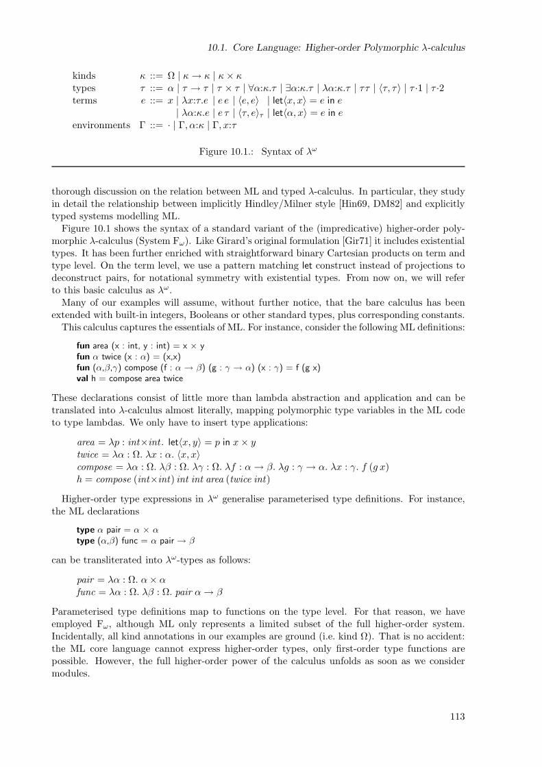
10.1. Core Language: Higher-order Polymorphic λ-calculus
kinds κ ::= Ω | κ→ κ | κ× κtypes τ ::= α | τ → τ | τ × τ | ∀α:κ.τ | ∃α:κ.τ | λα:κ.τ | ττ | 〈τ, τ〉 | τ ·1 | τ ·2terms e ::= x | λx:τ.e | e e | 〈e, e〉 | let〈x, x〉 = e in e
| λα:κ.e | e τ | 〈τ, e〉τ | let〈α, x〉 = e in eenvironments Γ ::= · | Γ, α:κ | Γ, x:τ
Figure 10.1.: Syntax of λω
thorough discussion on the relation between ML and typed λ-calculus. In particular, they studyin detail the relationship between implicitly Hindley/Milner style [Hin69, DM82] and explicitlytyped systems modelling ML.
Figure 10.1 shows the syntax of a standard variant of the (impredicative) higher-order poly-morphic λ-calculus (System Fω). Like Girard’s original formulation [Gir71] it includes existentialtypes. It has been further enriched with straightforward binary Cartesian products on term andtype level. On the term level, we use a pattern matching let construct instead of projections todeconstruct pairs, for notational symmetry with existential types. From now on, we will referto this basic calculus as λω.
Many of our examples will assume, without further notice, that the bare calculus has beenextended with built-in integers, Booleans or other standard types, plus corresponding constants.
This calculus captures the essentials of ML. For instance, consider the following ML definitions:
fun area (x : int, y : int) = x × yfun α twice (x : α) = (x,x)fun (α,β,γ) compose (f : α → β) (g : γ → α) (x : γ) = f (g x)val h = compose area twice
These declarations consist of little more than lambda abstraction and application and can betranslated into λ-calculus almost literally, mapping polymorphic type variables in the ML codeto type lambdas. We only have to insert type applications:
area = λp : int×int . let〈x, y〉 = p in x× ytwice = λα : Ω. λx : α. 〈x, x〉compose = λα : Ω. λβ : Ω. λγ : Ω. λf : α→ β. λg : γ → α. λx : γ. f (g x)h = compose (int×int) int int area (twice int)
Higher-order type expressions in λω generalise parameterised type definitions. For instance,the ML declarations
type α pair = α × αtype (α,β) func = α pair → β
can be transliterated into λω-types as follows:
pair = λα : Ω. α× αfunc = λα : Ω. λβ : Ω. pair α→ β
Parameterised type definitions map to functions on the type level. For that reason, we haveemployed Fω, although ML only represents a limited subset of the full higher-order system.Incidentally, all kind annotations in our examples are ground (i.e. kind Ω). That is no accident:the ML core language cannot express higher-order types, only first-order type functions arepossible. However, the full higher-order power of the calculus unfolds as soon as we considermodules.
113
10. A Calculus for Components
One noteworthy omission of the calculus when compared to the ML core language is theabsence of a fixed point operator. Unlike ML, bare Fω cannot express general recursion, so thatit in fact is terminating [Gir71, Bar92]. We do not add a primitive for recursion because thedynamic typing construct we will introduce in Section 10.4 actually allows expressing a fixedpoint operator for any inhabited type. It hence is unnecessary to make recursion primitive.
10.2. Modules: Existential Types and Higher-order Quantification
Modules play an important role in ML. Moreover, Alice ML’s dynamic typing facilities andcomponent system are centred around modules.
The ML module system has originally been proposed as a language based on dependenttypes [Mac86, Mac84]. That approach induces quite a heavyweight meta-theory, which had to betamed in a long line of work [HMM90, MT94, HL94, DCH03]. It has repeatedly been suggestedthat dependent types are overkill for representing modules, and that most of its features can besufficiently approximated in a simpler language based on a second-order calculus [Rus99]. Wehence follow more recent work [HMM90, Rus99, Dre05] and express modular structure in termsof λω with only moderate extensions.
The plain λω-calculus already is expressive enough to cover most of ML’s module language. Inparticular, the existential types of λω have a close correspondence to signatures: the signature
signature COMPLEX =sig
type complexval i : complexval mk : real → real → complexval re : complex → realval im : complex → realval mul : complex → complex → complex
end
can be interpreted as a λω-type as follows (reading × as a right-associative operator):
COMPLEX =∃complex : Ω. complex × (real → real → complex ) × (complex → real )
× (complex → real ) × (complex → complex → complex )
Signatures with more than one type can be expressed either by nested quantifiers, or in a moreregular manner, by quantification over product kinds [HS00]. For example,
signature GENERIC COMPLEX =sig
type basetype complexval i : complexval mk : base → base → complexval re : complex → baseval im : complex → baseval mul : complex → complex → complex
end
can be mapped to the type
GENERICCOMPLEX =∃〈base, complex 〉 : (Ω × Ω). (complex × (base → base → complex )
× (complex → base) × (complex → base)× (complex → complex → complex ))
114
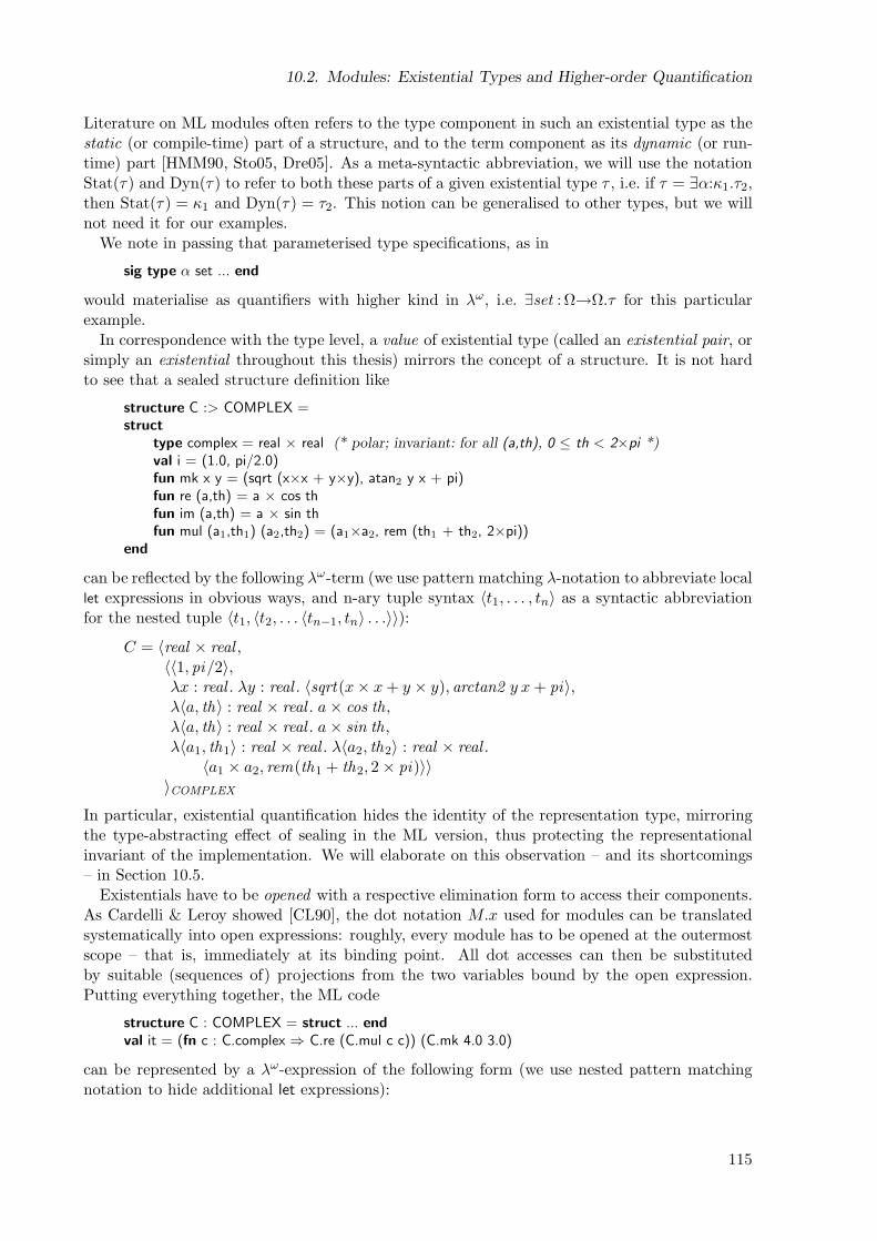
10.2. Modules: Existential Types and Higher-order Quantification
Literature on ML modules often refers to the type component in such an existential type as thestatic (or compile-time) part of a structure, and to the term component as its dynamic (or run-time) part [HMM90, Sto05, Dre05]. As a meta-syntactic abbreviation, we will use the notationStat(τ) and Dyn(τ) to refer to both these parts of a given existential type τ , i.e. if τ = ∃α:κ1.τ2,then Stat(τ) = κ1 and Dyn(τ) = τ2. This notion can be generalised to other types, but we willnot need it for our examples.
We note in passing that parameterised type specifications, as in
sig type α set ... end
would materialise as quantifiers with higher kind in λω, i.e. ∃set : Ω→Ω.τ for this particularexample.
In correspondence with the type level, a value of existential type (called an existential pair, orsimply an existential throughout this thesis) mirrors the concept of a structure. It is not hardto see that a sealed structure definition like
structure C :> COMPLEX =struct
type complex = real × real (* polar; invariant: for all (a,th), 0 ≤ th < 2×pi *)val i = (1.0, pi/2.0)fun mk x y = (sqrt (x×x + y×y), atan2 y x + pi)fun re (a,th) = a × cos thfun im (a,th) = a × sin thfun mul (a1,th1) (a2,th2) = (a1×a2, rem (th1 + th2, 2×pi))
end
can be reflected by the following λω-term (we use pattern matching λ-notation to abbreviate locallet expressions in obvious ways, and n-ary tuple syntax 〈t1, . . . , tn〉 as a syntactic abbreviationfor the nested tuple 〈t1, 〈t2, . . . 〈tn−1, tn〉 . . .〉〉):
C = 〈real × real ,〈〈1, pi/2〉,λx : real . λy : real . 〈sqrt(x× x+ y × y), arctan2 y x+ pi〉,λ〈a, th〉 : real × real . a× cos th,λ〈a, th〉 : real × real . a× sin th,λ〈a1, th1〉 : real × real . λ〈a2, th2〉 : real × real .
〈a1 × a2, rem(th1 + th2, 2 × pi)〉〉〉COMPLEX
In particular, existential quantification hides the identity of the representation type, mirroringthe type-abstracting effect of sealing in the ML version, thus protecting the representationalinvariant of the implementation. We will elaborate on this observation – and its shortcomings– in Section 10.5.
Existentials have to be opened with a respective elimination form to access their components.As Cardelli & Leroy showed [CL90], the dot notation M.x used for modules can be translatedsystematically into open expressions: roughly, every module has to be opened at the outermostscope – that is, immediately at its binding point. All dot accesses can then be substitutedby suitable (sequences of) projections from the two variables bound by the open expression.Putting everything together, the ML code
structure C : COMPLEX = struct ... end
val it = (fn c : C.complex ⇒ C.re (C.mul c c)) (C.mk 4.0 3.0)
can be represented by a λω-expression of the following form (we use nested pattern matchingnotation to hide additional let expressions):
115
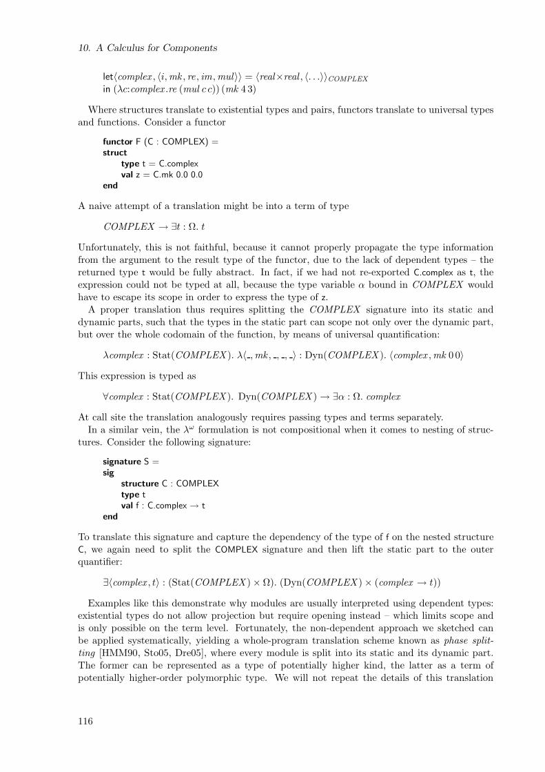
10. A Calculus for Components
let〈complex , 〈i,mk , re , im ,mul〉〉 = 〈real×real , 〈. . .〉〉COMPLEX
in (λc:complex .re (mul c c)) (mk 4 3)
Where structures translate to existential types and pairs, functors translate to universal typesand functions. Consider a functor
functor F (C : COMPLEX) =struct
type t = C.complexval z = C.mk 0.0 0.0
end
A naive attempt of a translation might be into a term of type
COMPLEX → ∃t : Ω. t
Unfortunately, this is not faithful, because it cannot properly propagate the type informationfrom the argument to the result type of the functor, due to the lack of dependent types – thereturned type t would be fully abstract. In fact, if we had not re-exported C.complex as t, theexpression could not be typed at all, because the type variable α bound in COMPLEX wouldhave to escape its scope in order to express the type of z.
A proper translation thus requires splitting the COMPLEX signature into its static anddynamic parts, such that the types in the static part can scope not only over the dynamic part,but over the whole codomain of the function, by means of universal quantification:
λcomplex : Stat(COMPLEX ). λ〈 ,mk , , , 〉 : Dyn(COMPLEX ). 〈complex ,mk 0 0〉
This expression is typed as
∀complex : Stat(COMPLEX ). Dyn(COMPLEX ) → ∃α : Ω. complex
At call site the translation analogously requires passing types and terms separately.In a similar vein, the λω formulation is not compositional when it comes to nesting of struc-
tures. Consider the following signature:
signature S =sig
structure C : COMPLEXtype tval f : C.complex → t
end
To translate this signature and capture the dependency of the type of f on the nested structureC, we again need to split the COMPLEX signature and then lift the static part to the outerquantifier:
∃〈complex , t〉 : (Stat(COMPLEX ) × Ω). (Dyn(COMPLEX ) × (complex → t))
Examples like this demonstrate why modules are usually interpreted using dependent types:existential types do not allow projection but require opening instead – which limits scope andis only possible on the term level. Fortunately, the non-dependent approach we sketched canbe applied systematically, yielding a whole-program translation scheme known as phase split-ting [HMM90, Sto05, Dre05], where every module is split into its static and its dynamic part.The former can be represented as a type of potentially higher kind, the latter as a term ofpotentially higher-order polymorphic type. We will not repeat the details of this translation
116
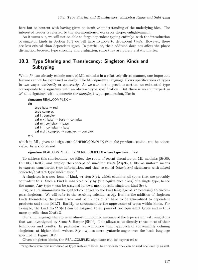
10.3. Type Sharing and Translucency: Singleton Kinds and Subtyping
here but be content with having given an intuitive understanding of the underlying idea. Theinterested reader is referred to the aforementioned works for deeper enlightenment.
As it turns out, we will not be able to forgo dependent typing entirely: with the introductionof singleton kinds in Section 10.3 we will have to move to dependent kinds. However, theseare less critical than dependent types. In particular, their addition does not affect the phasedistinction between type checking and evaluation, since they are purely a static matter.
10.3. Type Sharing and Translucency: Singleton Kinds and
Subtyping
While λω can already encode most of ML modules in a relatively direct manner, one importantfeature cannot be expressed as easily. The ML signature language allows specifications of typesin two ways: abstractly or concretely. As we saw in the previous section, an existential typecorresponds to a signature with an abstract type specification. But there is no counterpart inλω to a signature with a concrete (or manifest) type specification, like in
signature REAL COMPLEX =sig
type base = realtype complexval i : complexval mk : base → base → complexval re : complex → baseval im : complex → baseval mul : complex → complex → complex
end
which in ML, given the signature GENERIC COMPLEX from the previous section, can be abbre-viated by a short-hand:
signature REAL COMPLEX = GENERIC COMPLEX where type base = real
To address this shortcoming, we follow the route of recent literature on ML modules [Sto00,DCH03, Dre05], and employ the concept of singleton kinds [Asp95, SH06] as uniform meansto express transparent type information, and thus so-called translucent signatures with mixedconcrete/abstract type information.1
A singleton is a new form of kind, written S(τ), which classifies all types that are provablyequivalent to τ . Such a kind is inhabited only by (the equivalence class) of a single type, hencethe name. Any type τ can be assigned its own most specific singleton kind S(τ).
Figure 10.2 summarises the syntactic changes to the kind language of λω necessary to encom-pass singletons. We will refer to the resulting calculus as λω
S . Besides the addition of singletonkinds themselves, the plain arrow and pair kinds of λω have to be generalised to dependentproducts and sums [ML71, Bar92], to accommodate the appearance of types within kinds. Forexample, the kind Σα:Ω.S(α) can be assigned to all pairs of two equivalent types and is thusmore specific than Σα:Ω.Ω.
Our kind language thereby is an almost unmodified instance of the type system with singletonsthat was investigated by Stone & Harper [SH06]. This allows us to directly re-use most of theirtechniques and results. In particular, we will follow their approach of conveniently definingsingletons at higher kind, written S(τ : κ), as mere syntactic sugar over the basic languagespecified in Figure 10.2.
Given singleton kinds, the REAL COMPLEX signature can be expressed as
1Singletons were first introduced as types instead of kinds, but obviously they can be used one level up as well.
117
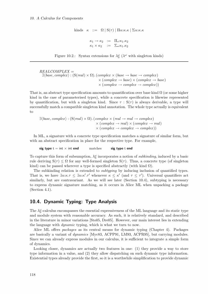
10. A Calculus for Components
kinds κ ::= Ω | S(τ) | Πα:κ.κ | Σα:κ.κ
κ1 → κ2 := Π :κ1.κ2
κ1 × κ2 := Σ :κ1.κ2
Figure 10.2.: Syntax extensions for λωS (λω with singleton kinds)
REALCOMPLEX =∃〈base, complex 〉 : (S(real ) × Ω). (complex × (base → base → complex )
× (complex → base) × (complex → base)× (complex → complex → complex ))
That is, an abstract type specification amounts to quantification over base kind Ω (or some higherkind in the case of parameterised types), while a concrete specification is likewise representedby quantification, but with a singleton kind. Since τ : S(τ) is always derivable, a type willsuccessfully match a compatible singleton kind annotation. The whole type actually is equivalentto
∃〈base, complex 〉 : (S(real ) × Ω). (complex × (real → real → complex )× (complex → real ) × (complex → real )× (complex → complex → complex ))
In ML, a signature with a concrete type specification matches a signature of similar form, butwith an abstract specification in place for the respective type. For example,
sig type t = int × int end matches sig type t end
To capture this form of subsumption, λωS incorporates a notion of subkinding, induced by a basic
rule deriving S(τ) ≤ Ω for any well-formed singleton S(τ). Thus, a concrete type (of singletonkind) can be passed wherever a type is specified abstractly (with kind Ω).
The subkinding relation is extended to subtyping by inducing inclusion of quantified types.That is, we have ∃α:κ.τ ≤ ∃α:κ′.τ ′ whenever κ ≤ κ′ (and τ ≤ τ ′). Universal quantifiers actsimilarly, but are contravariant. As we will see later (Section 10.4), subtyping is necessaryto express dynamic signature matching, as it occurs in Alice ML when unpacking a package(Section 4.1).
10.4. Dynamic Typing: Type Analysis
The λωS -calculus encompasses the essential expressiveness of the ML language and its static type
and module system with reasonable accuracy. As such, it is relatively standard, and describedin the literature in minor variations [Sto05, Dre05]. However, our main interest lies in extendingthe language with dynamic typing, which is what we turn to now.
Alice ML offers packages as its central means for dynamic typing (Chapter 4). Packagesare basically a variant of dynamics [Myc83, ACPP91, LM93, ACPR95], but carrying modules.Since we can already express modules in our calculus, it is sufficient to integrate a simple formof dynamics.
Looking closer, dynamics are actually two features in one: (1) they provide a way to storetype information in a value, and (2) they allow dispatching on such dynamic type information.Existential types already provide the first, so it is a worthwhile simplification to provide dynamic
118
10.4. Dynamic Typing: Type Analysis
type switching as a separate feature, and express dynamics in terms of these two, more primitivemechanisms.
Like dynamics, dynamic type analysis has been investigated extensively in literature [HM95,DRW95, Gle99, CW99, TSS00, Wei02, CWM02, VWW05]. Most of these works introduce atypecase construct of varying complexity for dispatching on the structure of a type, sometimesalong with a similar construct typerec on the type level, to encompass higher-order types.
We restrict ourselves to a much simpler construct, which just provides a way to compare twotypes, and branch according to the result:
case e1:τ1 of x:τ2.e2 else e3
Evaluating this expression compares the dynamic instantiations of the type τ1 of value e1 withτ2. If they match, the e2 branch is taken, with x bound to the value of e1, otherwise e3 isevaluated. However, the comparison is not for type equivalence, but for subtyping ! That is, ifτ1 ≤ τ2 then e2 is chosen. In other words, our type case is reminiscent of a checked downcast.More formally, it is a variant of Girard’s J operator [Gir71], or rather Harper & Mitchell’sTypeCond operator [HM99], enriched with subtyping (Section 12.3.3).
Given a primitive for dynamic type analysis, an equivalent to the Alice ML package type canbe defined in our system as ∃α:Ω.α, which we will abbreviate to package in the following. Theintuition is obvious: a package is a value of some type named α, paired with the actual type. Theequivalent to injecting some value into type package hence is nothing more than plain existentialconstruction.
Consider the following Alice ML example:
val p = pack (val it = 5) : (val it : int)
The straightforward translation is
p = 〈int , 5〉package
This scales to more complex modules in the obvious way. For instance, here is a module includinga type:
val q = pack (type t = int; fun f (n : int) = n) : (type t = int; val f : t → t)
It could be expressed as follows:
q = 〈∃t : S(int). t→ t, 〈int , λn : int . n〉∃t:S(int)〉package
Note the twofold use of existential types in this example: the inner existential expresses thestructure, the outer the package.
Since constructing a package obviously is straightforward, unpacking is the more interestingdirection: given a value of package type and a target signature (cf. Section 4.1) it should yieldthe contained module, if and only if the dynamic signature is a subtype of the target signature.Consider the following piece of Alice ML code:
unpack p : (val it : int)
It is not difficult to express this operation in terms of existential opening and type case:
let〈α, x′〉 = p in casex′ : α of x : int . x else ⊥int
Because we do not have exceptions in the calculus, we use ⊥ to indicate the exceptional case(we will see in Section 12.3.3 that we can find a diverging computation for all interesting types).
The second of the above packages, q, can be unpacked successfully in at least two differentways:
119
10. A Calculus for Components
structure M1 = unpack q : (type t = int; val f : t → t)structure M2 = unpack q : (type t; val f : t → t)
M1 unpacks it under its original, most precise signature. M2 however uses a supersignature wheret is left abstract. Both can be translated directly:
M1 = let〈α,M ′〉 = q in caseM ′ : α of M : (∃t : S(int). t→ t). M else ⊥M2 = let〈α,M ′〉 = q in caseM ′ : α of M : (∃t : Ω. t→ t). M else ⊥
The latter example demonstrates why we needed to built in subtyping (Section 10.3) into ourcalculus: the case expression in M2 does only evaluate successfully because ∃t : S(int). t → t ≤∃t : Ω. t→ t. Unlike static uses of subsumption [Sto05, Dre05], we cannot express the conversionbetween these types by η-expansion, because the package type is not statically known.
10.5. Loss of Parametricity and Abstraction Safety
Although the type case construct may look rather innocent at first, it has serious implica-tions on the properties of the calculus. As said above, it represents a variant of Girard’s Jcombinator [Gir71, HM99], and Girard showed that such an operator inherently destroys theparametricity property of the polymorphic λ-calculus.
Intuitively, parametricity means that a well-formed term always reduces in the same way,regardless of potential substitution of free type variables [Rey83, BFSS89, ACC93]. Obviously,a type case enables inspection of the dynamic instantiation of a type variable, and it can evaluateto different branches, accordingly.
As already explained in Section 4.5, a number of useful properties are consequences of para-metricity, and they get lost along the way. For example, unlike λω, the extended calculus isnot terminating (Section 12.3.3). More seriously, though, type abstraction can no longer beexpressed by conventional means.
Type abstraction is one of the most important tools of modular programming [Mor73a,Mor73b, MP88, HP05]. In the ML module system type abstraction is achieved through sealing(Chapter 3): the representation of a type defined by a structure is hidden to clients by ascribinga signature containing an abstract type specification. For example, recall our structure definingcomplex numbers:
signature COMPLEX =sig
type complexval i : complexval mk : real → real → complexval re : complex → realval im : complex → realval mul : complex → complex → complex
end
structure C :> COMPLEX =struct
type complex = real × real (* polar; invariant: for all (a,th), ≤ th < 2×pi *)val i = (1.0, pi/2.0)fun mk x y = (sqrt (x×x + y×y), atan2 y x + pi)fun re (a,th) = a × cos thfun im (a,th) = a × sin thfun mul (a1,th1) (a2,th2) = (a1×a2, rem (th1 + th2, 2×pi))
end
120
10.5. Loss of Parametricity and Abstraction Safety
This declaration defines an abstract type C.complex, whose representation is hidden from clients– they can only use the operations from the COMPLEX signature to construct, consume, andinspect values of this type.
If the language provides no way to breach an abstraction barrier erected through the use ofabstract types it is called abstraction safe. Standard ML and most similar languages have thisproperty.
In their classic paper, Mitchell & Plotkin observed that type abstraction is closely relatedto existential quantification [MP88]. In Section 10.2, we already saw how the complex numberADT can be expressed in λω as an existential:
C = 〈real × real ,〈〈1, pi/2〉,λx : real . λy : real . 〈sqrt(x× x+ y × y), arctan2 y x+ pi〉,λ〈a, th〉 : real × real . a× cos th,λ〈a, th〉 : real × real . a× sin th,λ〈a1, th1〉 : real × real . λ〈a2, th2〉 : real × real .
〈a1 × a2, rem(th1 + th2, 2 × pi)〉〉〉COMPLEX
Abstraction safety in this approach crucially relies on parametricity. To be accessed, theexistential has to be opened, as in
let〈γ, ops〉 = C in e
But only because the body e – which represents the client code of the structure – is parametricin the bound type variable γ representing the abstract type complex , it is guaranteed not to beable to break the abstraction: it simply cannot perform any computations that depend on therepresentation of γ, i.e. the concrete type that will be substituted during reduction.
Unfortunately, the loss of parametricity caused by the addition of dynamic type analysis inval-idates this solely static model of type abstraction. Specifically, we can construct an expressionthat breaks the abstraction of the complex number ADT by dynamically inspecting the abstracttype and consecutively constructing a value of the abstract type without using the mk operatorfrom its signature:
let〈γ, ops〉 = C in . . . case 〈0,−3 × pi〉 : real × real of x : γ. x else i . . .
The type case in this expression is perfectly well-typed. Dynamically, it checks whether real×realand the abstract type γ are equivalent, and in case they are, interprets the pair 〈0,−3 × pi〉as a complex value. And the check will indeed succeed, because the reduction rule for the let
expression opening the existential will substitute γ by real × real , implying γ ≡ real × real . Byevaluating this expression, we have forged a value of the abstract type for complex numbers.Note that indeed, 〈0,−3× pi〉 does not adhere to the intended invariant of the implementation,which would require −3π ∈ [0; 2π[.
There seem to be two principal ways to restore abstraction safety in the presence of dynamictype analysis:
1. Disallow dynamic analysis of certain types. This approach has been suggested by Harper& Morrisett [HM95], who propose statically distinguishing between analysable and non-analysable types, supposedly via the kind system.
2. Prevent substitution of (existentially) quantified types. Abadi, Cardelli, Pierce & Remy[ACPR95] propose to simply replacing the type variable bound by open with a “fresh”type constant during evaluation.
121
10. A Calculus for Components
The first solution is overly restrictive for our purposes, because it would preclude valuesof certain types – specifically, all abstract types – to be put in packages. Clearly, such alimitation would render packages insufficient as a basis for a component system. We need a fullreflexivity type analysis mechanism, i.e. all types have to be analysable – or rather, comparable– dynamically.2
The idea put forth by Abadi et al. is more promising. It amounts to changing the reductionrule for opening existientials to:
let〈α, x〉 = 〈τ, v〉 in e → e[t/α][v/x]
where t is a fresh type constant. Obviously, the representation type could no longer be analysedtransparently.
Unfortunately, this modification has two fundamental problems:
• The notion of “fresh type constant” is not formally defined. It needs to be made precisewhat dynamic freshness means.
• Worse, the rule destroys type preservation.
To see how type preservation is lost, consider the following example:
let〈complex , 〈i,mk , re , im ,mul〉〉 = C in (λc : complex . re c) i
It is easy to verify that this term is well-typed in λω . Nevertheless, after applying the abovereduction rule (and the implicit deconstructions of the nested operator tuple) the term becomes:
(λc : t. (λ〈a, th〉 : real × real . a× cos th) c) 〈1, pi/2〉
which is no longer typable! In two places there is a clash between the abstract type t – whichnow stands for complex – and its representation type real ×real : the tuple 〈1, pi/2〉 representingthe complex number i simply has type real × real where the outer λ-expression expects t, andvice versa, c has type t where the implementation of the re function expects a pair.
The approach we are going to present in the following takes up the idea of generating freshtypes to maintain abstraction safety, but avoiding the above problems:
• Instead of “fresh type constants” it introduces an explicit construct for dynamically gen-erating type names, independent from existential types.
• Type inconsistencies between abstract types and their representations are addressed byintroducing coercions for mitigating between the types.
The basic approach has been described previously in a paper of ours [Ros03]. However, in thepaper we did not consider the interaction with singleton kinds and the resulting dependencyof kinds on types, which turns out to be a severe complication. Moreover, the current workfeatures a more modular approach to recording the isomorphism between generated types andtheir representations, by using the kind system. It also simplifies higher-order coercions bytreating them as syntactic sugar.
2We borrow the term full reflexivity from Trifonov, Saha & Shao [TSS00], who introduced it in a slightly differentcontext to express the absence of any restriction on the syntactic form of types that are available for analysis(no such restriction is necessary for the simple form of type case used in this thesis).
122
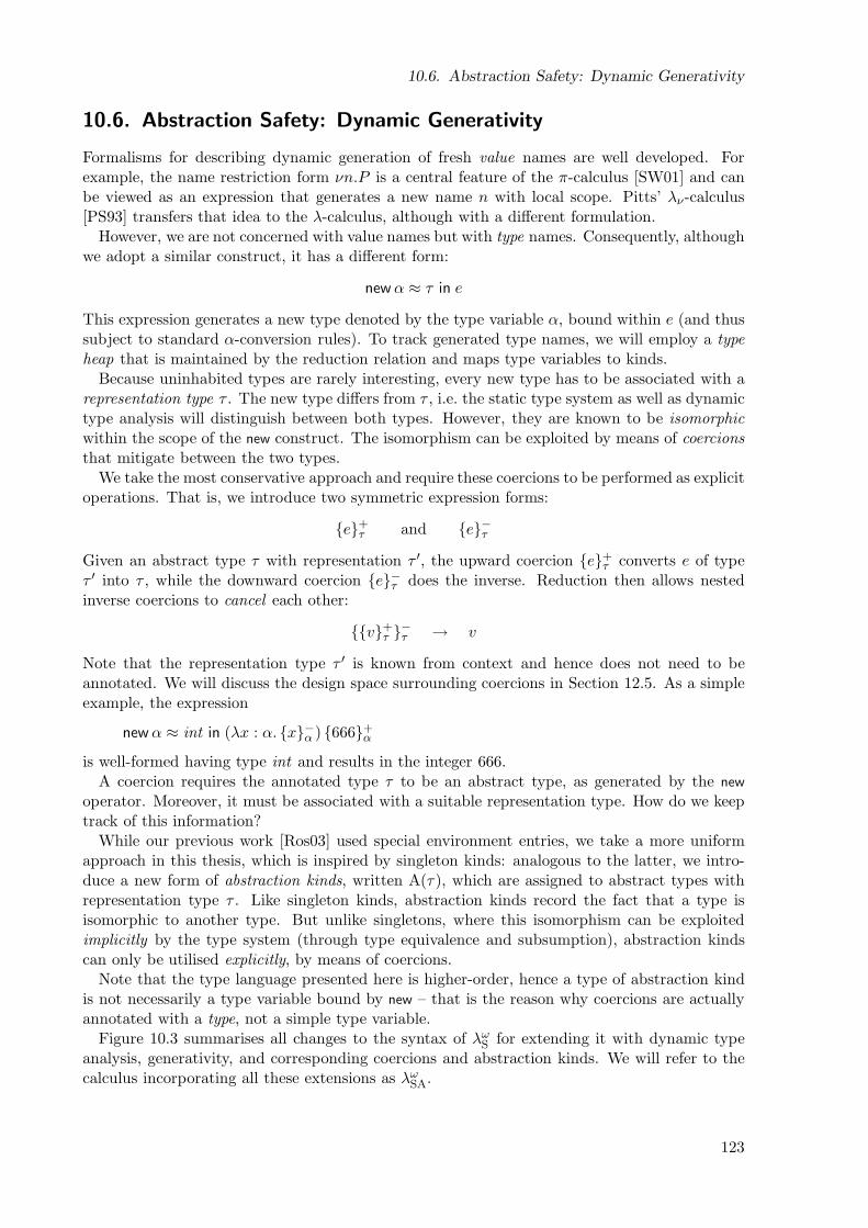
10.6. Abstraction Safety: Dynamic Generativity
10.6. Abstraction Safety: Dynamic Generativity
Formalisms for describing dynamic generation of fresh value names are well developed. Forexample, the name restriction form νn.P is a central feature of the π-calculus [SW01] and canbe viewed as an expression that generates a new name n with local scope. Pitts’ λν-calculus[PS93] transfers that idea to the λ-calculus, although with a different formulation.
However, we are not concerned with value names but with type names. Consequently, althoughwe adopt a similar construct, it has a different form:
newα ≈ τ in e
This expression generates a new type denoted by the type variable α, bound within e (and thussubject to standard α-conversion rules). To track generated type names, we will employ a typeheap that is maintained by the reduction relation and maps type variables to kinds.
Because uninhabited types are rarely interesting, every new type has to be associated with arepresentation type τ . The new type differs from τ , i.e. the static type system as well as dynamictype analysis will distinguish between both types. However, they are known to be isomorphicwithin the scope of the new construct. The isomorphism can be exploited by means of coercionsthat mitigate between the two types.
We take the most conservative approach and require these coercions to be performed as explicitoperations. That is, we introduce two symmetric expression forms:
e+τ and e−τ
Given an abstract type τ with representation τ ′, the upward coercion e+τ converts e of type
τ ′ into τ , while the downward coercion e−τ does the inverse. Reduction then allows nestedinverse coercions to cancel each other:
v+τ
−τ → v
Note that the representation type τ ′ is known from context and hence does not need to beannotated. We will discuss the design space surrounding coercions in Section 12.5. As a simpleexample, the expression
newα ≈ int in (λx : α. x−α ) 666+α
is well-formed having type int and results in the integer 666.A coercion requires the annotated type τ to be an abstract type, as generated by the new
operator. Moreover, it must be associated with a suitable representation type. How do we keeptrack of this information?
While our previous work [Ros03] used special environment entries, we take a more uniformapproach in this thesis, which is inspired by singleton kinds: analogous to the latter, we intro-duce a new form of abstraction kinds, written A(τ), which are assigned to abstract types withrepresentation type τ . Like singleton kinds, abstraction kinds record the fact that a type isisomorphic to another type. But unlike singletons, where this isomorphism can be exploitedimplicitly by the type system (through type equivalence and subsumption), abstraction kindscan only be utilised explicitly, by means of coercions.
Note that the type language presented here is higher-order, hence a type of abstraction kindis not necessarily a type variable bound by new – that is the reason why coercions are actuallyannotated with a type, not a simple type variable.
Figure 10.3 summarises all changes to the syntax of λωS for extending it with dynamic type
analysis, generativity, and corresponding coercions and abstraction kinds. We will refer to thecalculus incorporating all these extensions as λω
SA.
123
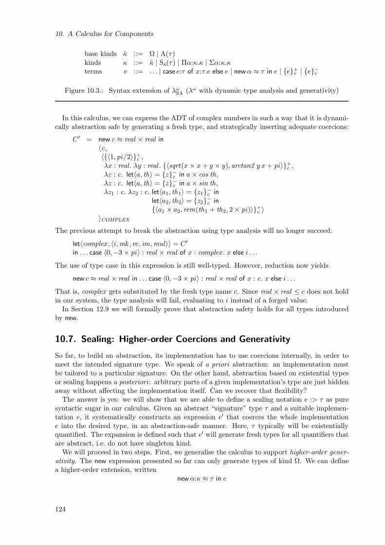
10. A Calculus for Components
base kinds κ ::= Ω | A(τ)kinds κ ::= κ | Sκ(τ) | Πα:κ.κ | Σα:κ.κterms e ::= . . . | case e:τ of x:τ.e else e | newα ≈ τ in e | e+
τ | e−τ
Figure 10.3.: Syntax extension of λωSA (λω with dynamic type analysis and generativity)
In this calculus, we can express the ADT of complex numbers in such a way that it is dynami-cally abstraction safe by generating a fresh type, and strategically inserting adequate coercions:
C ′ = new c ≈ real × real in〈c,〈〈1, pi/2〉+
c ,λx : real . λy : real . 〈sqrt(x× x+ y × y), arctan2 y x+ pi〉+
c ,λz : c. let〈a, th〉 = z−c in a× cos th,λz : c. let〈a, th〉 = z−c in a× sin th,λz1 : c. λz2 : c. let〈a1, th1〉 = z1
−c in
let〈a2, th2〉 = z2−c in
〈a1 × a2, rem(th1 + th2, 2 × pi)〉+c 〉
〉COMPLEX
The previous attempt to break the abstraction using type analysis will no longer succeed:
let〈complex , 〈i,mk , re , im ,mul〉〉 = C ′
in . . . case 〈0,−3 × pi〉 : real × real of x : complex . x else i . . .
The use of type case in this expression is still well-typed. However, reduction now yields
new c ≈ real × real in . . . case 〈0,−3 × pi〉 : real × real of x : c. x else i . . .
That is, complex gets substituted by the fresh type name c. Since real × real ≤ c does not holdin our system, the type analysis will fail, evaluating to i instead of a forged value.
In Section 12.9 we will formally prove that abstraction safety holds for all types introducedby new.
10.7. Sealing: Higher-order Coercions and Generativity
So far, to build an abstraction, its implementation has to use coercions internally, in order tomeet the intended signature type. We speak of a priori abstraction: an implementation mustbe tailored to a particular signature. On the other hand, abstraction based on existential typesor sealing happens a posteriori : arbitrary parts of a given implementation’s type are just hiddenaway without affecting the implementation itself. Can we recover that flexibility?
The answer is yes: we will show that we are able to define a sealing notation e :> τ as puresyntactic sugar in our calculus. Given an abstract “signature” type τ and a suitable implemen-tation e, it systematically constructs an expression e′ that coerces the whole implementatione into the desired type, in an abstraction-safe manner. Here, τ typically will be existentiallyquantified. The expansion is defined such that e′ will generate fresh types for all quantifiers thatare abstract, i.e. do not have singleton kind.
We will proceed in two steps. First, we generalise the calculus to support higher-order gener-ativity. The new expression presented so far can only generate types of kind Ω. We can definea higher-order extension, written
newα:κ ≈ τ in e
124
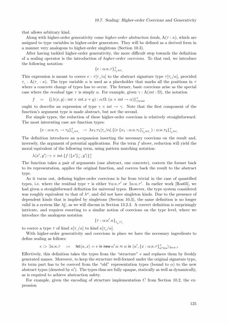
10.7. Sealing: Higher-order Coercions and Generativity
that allows arbitrary kind.Along with higher-order generativity come higher-order abstraction kinds, A(τ : κ), which are
assigned to type variables in higher-order generators. They will be defined as a derived form ina manner very analogous to higher-order singletons (Section 10.3).
After having tackled higher-order generativity, the more difficult step towards the definitionof a sealing operator is the introduction of higher-order coercions. To that end, we introducethe following notation:
e : α:κ.τ+τ+≈τ−
This expression is meant to coerce e : τ [τ−/α] to the abstract signature type τ [τ+/α], provided
τ+
: A(τ− : κ). The type variable α is used as a placeholder that marks all the positions in τwhere a concrete change of types has to occur. The former, basic coercions arise as the specialcase where the residual type τ is simply α. For example, given γ : A(int : Ω), the notation
f = (λ〈x, y〉 : int × int .x+ y) : α:Ω. (α× int → α)+γ≈int
ought to describe an expression of type γ × int → γ. Note that the first component of thefunction’s argument type is made abstract, but not the second.
For simple types, the reduction of these higher-order coercions is relatively straightforward.The most interesting case are function types:
v : α:κ.τ1 → τ2+τ+≈τ−
→ λx1:τ1[τ+/α].(v x1 : α:κ.τ1−τ+≈τ−
) : α:κ.τ2+τ+≈τ−
The definition introduces an η-expansion inserting the necessary coercions on the result and,inversely, the argument of potential applications. For the term f above, reduction will yield themoral equivalent of the following term, using pattern matching notation:
λ〈x′, y′〉 : γ × int .f 〈x′−γ , y′〉+
γ
The function takes a pair of arguments (one abstract, one concrete), coerces the former backto its representation, applies the original function, and coerces back the result to the abstracttype.
As it turns out, defining higher-order coercions is far from trivial in the case of quantifiedtypes, i.e. where the residual type τ is either ∀α:κ.τ ′ or ∃α:κ.τ ′. In earlier work [Ros03], wehad given a straightforward definition for universal types. However, the type system consideredwas roughly equivalent to that of λω, and did not have singleton kinds. Due to the presence ofdependent kinds that is implied by singletons (Section 10.3), the same definition is no longervalid in a system like λω
S , as we will discuss in Section 13.2.3. A correct definition is surprisinglyintricate, and requires resorting to a similar notion of coercions on the type level, where weintroduce the analogous notation
τ : α:κ′.κτ+
/τ−
to coerce a type τ of kind κ[τ−/α] to kind κ[τ+/α].
With higher-order generativity and coercions in place we have the necessary ingredients todefine sealing as follows:
e :> ∃α:κ.τ := let〈α, x〉 = e in newα′:κ ≈ α in 〈α′, x : α:κ.τ+α′≈α〉∃α:κ.τ
Effectively, this definition takes the types from the “structure” e and replaces them by freshlygenerated names. Moreover, to keep the structure well-formed under the original signature type,its term part has to be coerced from the “old” representation types (bound to α) to the newabstract types (denoted by α′). The types thus are fully opaque, statically as well as dynamically,as is required to achieve abstraction safety.
For example, given the encoding of structure implementation C from Section 10.2, the ex-pression
125
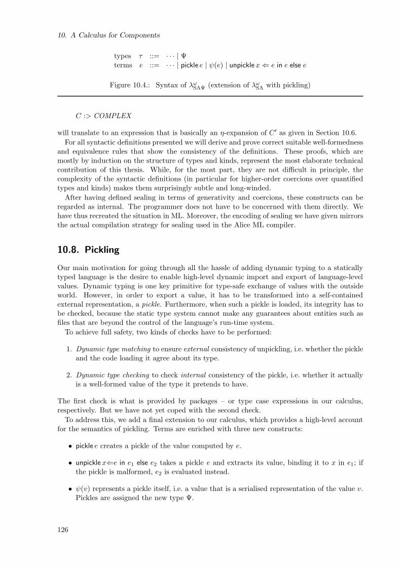
10. A Calculus for Components
types τ ::= · · · | Ψterms e ::= · · · | pickle e | ψ(e) | unpicklex⇐ e in e else e
Figure 10.4.: Syntax of λωSAΨ (extension of λω
SA with pickling)
C :> COMPLEX
will translate to an expression that is basically an η-expansion of C ′ as given in Section 10.6.
For all syntactic definitions presented we will derive and prove correct suitable well-formednessand equivalence rules that show the consistency of the definitions. These proofs, which aremostly by induction on the structure of types and kinds, represent the most elaborate technicalcontribution of this thesis. While, for the most part, they are not difficult in principle, thecomplexity of the syntactic definitions (in particular for higher-order coercions over quantifiedtypes and kinds) makes them surprisingly subtle and long-winded.
After having defined sealing in terms of generativity and coercions, these constructs can beregarded as internal. The programmer does not have to be concerned with them directly. Wehave thus recreated the situation in ML. Moreover, the encoding of sealing we have given mirrorsthe actual compilation strategy for sealing used in the Alice ML compiler.
10.8. Pickling
Our main motivation for going through all the hassle of adding dynamic typing to a staticallytyped language is the desire to enable high-level dynamic import and export of language-levelvalues. Dynamic typing is one key primitive for type-safe exchange of values with the outsideworld. However, in order to export a value, it has to be transformed into a self-containedexternal representation, a pickle. Furthermore, when such a pickle is loaded, its integrity has tobe checked, because the static type system cannot make any guarantees about entities such asfiles that are beyond the control of the language’s run-time system.
To achieve full safety, two kinds of checks have to be performed:
1. Dynamic type matching to ensure external consistency of unpickling, i.e. whether the pickleand the code loading it agree about its type.
2. Dynamic type checking to check internal consistency of the pickle, i.e. whether it actuallyis a well-formed value of the type it pretends to have.
The first check is what is provided by packages – or type case expressions in our calculus,respectively. But we have not yet coped with the second check.
To address this, we add a final extension to our calculus, which provides a high-level accountfor the semantics of pickling. Terms are enriched with three new constructs:
• pickle e creates a pickle of the value computed by e.
• unpicklex⇐e in e1 else e2 takes a pickle e and extracts its value, binding it to x in e1; ifthe pickle is malformed, e2 is evaluated instead.
• ψ(v) represents a pickle itself, i.e. a value that is a serialised representation of the value v.Pickles are assigned the new type Ψ.
126
10.9. Summary
Figure 10.4 summarises the extensions. We refer to the resulting calculus as λωSAΨ.
The key characteristic of the pickling formalism is that there is no requirement for the term vin a pickle ψ(v) to actually be well-formed! This models the fact that in practice, pickles can becreated outside the runtime, by extra-linguistic means, and the language has no way to enforcethat they are well-formed. Indeed, a pickle may be deliberately forged by an attacker (in a reallanguage, a pickle might not even be syntactically valid, but we abstract from that possibilityin our calculus, since it does not change the principle problem). This liberty is visible in thetyping rule for pickles, which will have the following form:
Γ ⊢
Γ ⊢ ψ(v) : Ψ(FV(v) ⊆ Dom(Γ))
This rule does not have any premise regarding v, except that it has to be closed with respect tothe environment (this side condition is needed for technical ease only, namely to maintain thecalculus’ usual Type Variable Containment lemma, which says that a well-formed term containsno unbound variables).
If pickles may be malformed, how can we establish soundness? This requires verification whena pickle is loaded. In our model, verification simply amounts to a well-formedness side conditionin the reduction rules for unpickle:
unpicklex⇐ ψ(v) in e1 else e2 → e1[v/x] if Γ ⊢ v : package
unpicklex⇐ ψ(v) in e1 else e2 → e2 otherwise
Upon deconstruction, it is checked that a pickle actually contains a well-formed representationof a value of package type package (Section 10.4). As we will explain in Section 12.4.2, theenvironment Γ is needed to capture previously generated types, as these may occur within apickle. Except for those, Γ is empty, reflecting the requirement that a pickle be a closed value.
Despite the robustness achieved by run-time verification, we want to preclude that malformedpickles can be created from within the language. A programmer has to invoke pickle e to createpickles – the form ψ(v) should be considered inaccessible in the surface language. A pickleexpression first evaluates its operand e and then creates a pickle from the result. Unlike thevalues in a pickle, the type system requires the operand e to be a well-formed term.
Note that we do not actually model processes: neither does our calculus have concurrency(which is orthogonal to the issues discussed here), nor does it encompass local state. The onlybit of state existent in our calculus is the heap of generated types, which simply acts as beingglobal to all computation. This is a simplifying assumption that does not reflect the practicallanguage, but abstracts from distracting detail that does not seem to add much technical insightto the problem at hand.
Also for simplicity, our calculus does not model resources either. An account for resources inthe spirit of Alice ML would be relatively straightforward to add: it amounts to extending thepickle operator to conditional form and adding a side condition to its primary reduction rule thatensures that no resource names occur in v. Resources themselves could simply be representedas names drawn from a specific set.
10.9. Summary
• The λωSAΨ-calculus models the essentials of the Alice ML type system.
• This includes dynamic type matching, type generativity, type sharing, and pickling.
• It is based on the higher-order polymorphic λ-calculus (System Fω).
127
10. A Calculus for Components
• Singletons express type sharing.
• Type analysis expresses dynamic typing.
• Type generativity is an explicit construct.
• Coercions are used to switch between abstract types and their representation.
• Pickling delays well-formedness checks for terms until reduction.
128
11. The Type Language
The λωSAΨ-calculus incorporates an expressive static type system as well as non-trivial means of
dynamic typing. In this chapter we discuss the language of types and its properties.
We will first give an overview of the type system. Most of it is standard, except for singletonand abstraction kinds. We will hence concentrate on those, first giving a recap of singletons andtheir implications and then discussing design issues surrounding abstraction kinds, which areclosely related to singletons in most ways.
We state a number of relevant properties of the system. In the last section, we give algorithmicformulations of all judgements of the system, which are correct and decidable. We will needthis result when we turn to the semantics of type case in Chapter 12. We only state the maintheorems and propositions in this chapter. Auxiliary propositions and lemmata and all proofscan be found in Appendix C.
Most of what we discuss in this chapter is covered in literature, such that we can keep thediscussion brief and concentrate on the most interesting issues. As far as the type language isconcerned, abstraction kinds are the primary innovation over previous work.
11.1. Basic System
The abstract syntax of λωSAΨ is shown in Figure 11.1. As usual, we identify phrases (terms,
types, and kinds) up to renaming of bound variables. Except where noted otherwise, we alsouse the distinct variable convention, whereby all bound variables in a phrase are assumed to bedistinct from each other, and from any occurring free variable.
We write FV(t) for the set of free variables (including term and type variables) in the phrase t,defined as usual. We use the notation t[t′/z] for the capture-avoiding substitution of the phraset′ for the variable z in the phrase t. Moreover, we use γ to range over finite substitutions andwrite γ(t) for the capture-free application of such a substitution to a phrase t.
The static semantics of the calculus consists of eight judgements:
(environment validity) Γ ⊢ (kind validity) Γ ⊢ κ : (kind equivalence) Γ ⊢ κ ≡ κ′ : (kind inclusion) Γ ⊢ κ ≤ κ′ : (type validity) Γ ⊢ τ : κ(type equivalence) Γ ⊢ τ ≡ τ ′ : κ(type inclusion) Γ ⊢ τ ≤ τ ′ : κ(term validity) Γ ⊢ e : τ
Figures 11.2 to 11.6 show the inference rules defining the these judgements, except for termvalidity, which we delay until Chapter 12.
129
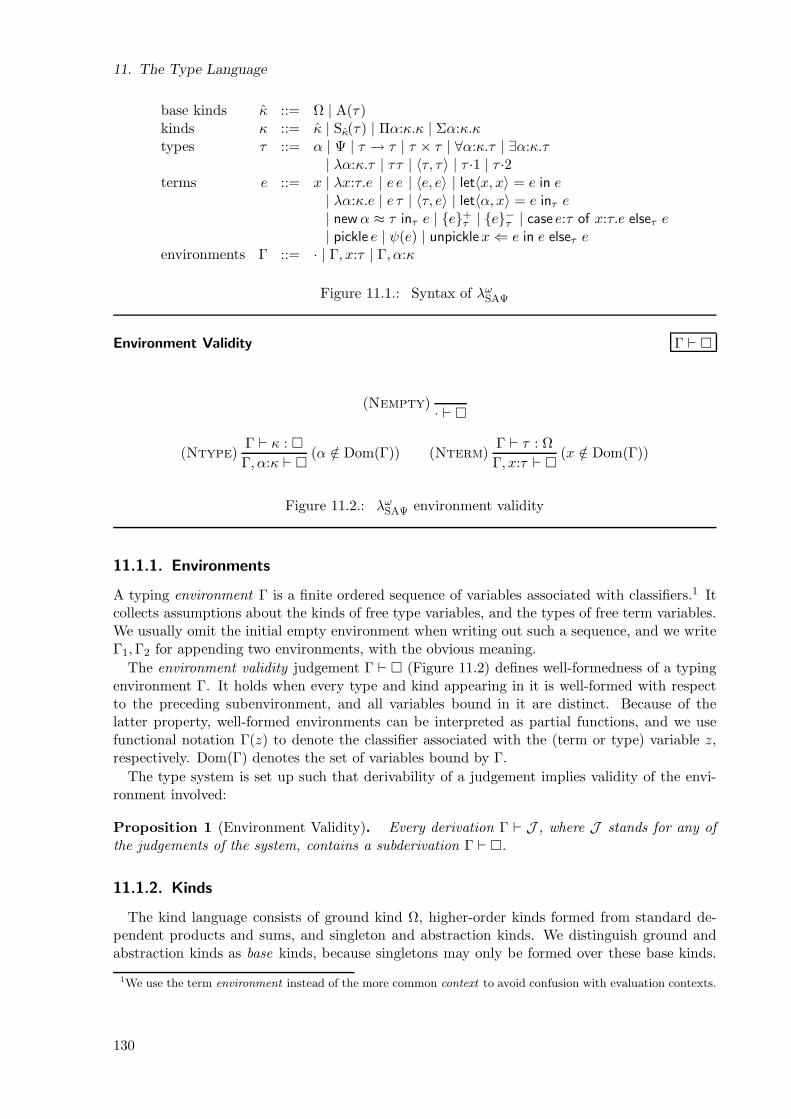
11. The Type Language
base kinds κ ::= Ω | A(τ)kinds κ ::= κ | Sκ(τ) | Πα:κ.κ | Σα:κ.κtypes τ ::= α | Ψ | τ → τ | τ × τ | ∀α:κ.τ | ∃α:κ.τ
| λα:κ.τ | ττ | 〈τ, τ〉 | τ ·1 | τ ·2terms e ::= x | λx:τ.e | e e | 〈e, e〉 | let〈x, x〉 = e in e
| λα:κ.e | e τ | 〈τ, e〉 | let〈α, x〉 = e inτ e| newα ≈ τ inτ e | e
+τ | e−τ | case e:τ of x:τ.e elseτ e
| pickle e | ψ(e) | unpicklex⇐ e in e elseτ eenvironments Γ ::= · | Γ, x:τ | Γ, α:κ
Figure 11.1.: Syntax of λωSAΨ
Environment Validity Γ ⊢
(Nempty)· ⊢
(Ntype)Γ ⊢ κ :
Γ, α:κ ⊢ (α /∈ Dom(Γ)) (Nterm)
Γ ⊢ τ : Ω
Γ, x:τ ⊢ (x /∈ Dom(Γ))
Figure 11.2.: λωSAΨ environment validity
11.1.1. Environments
A typing environment Γ is a finite ordered sequence of variables associated with classifiers.1 Itcollects assumptions about the kinds of free type variables, and the types of free term variables.We usually omit the initial empty environment when writing out such a sequence, and we writeΓ1,Γ2 for appending two environments, with the obvious meaning.
The environment validity judgement Γ ⊢ (Figure 11.2) defines well-formedness of a typingenvironment Γ. It holds when every type and kind appearing in it is well-formed with respectto the preceding subenvironment, and all variables bound in it are distinct. Because of thelatter property, well-formed environments can be interpreted as partial functions, and we usefunctional notation Γ(z) to denote the classifier associated with the (term or type) variable z,respectively. Dom(Γ) denotes the set of variables bound by Γ.
The type system is set up such that derivability of a judgement implies validity of the envi-ronment involved:
Proposition 1 (Environment Validity). Every derivation Γ ⊢ J , where J stands for any ofthe judgements of the system, contains a subderivation Γ ⊢ .
11.1.2. Kinds
The kind language consists of ground kind Ω, higher-order kinds formed from standard de-pendent products and sums, and singleton and abstraction kinds. We distinguish ground andabstraction kinds as base kinds, because singletons may only be formed over these base kinds.
1We use the term environment instead of the more common context to avoid confusion with evaluation contexts.
130
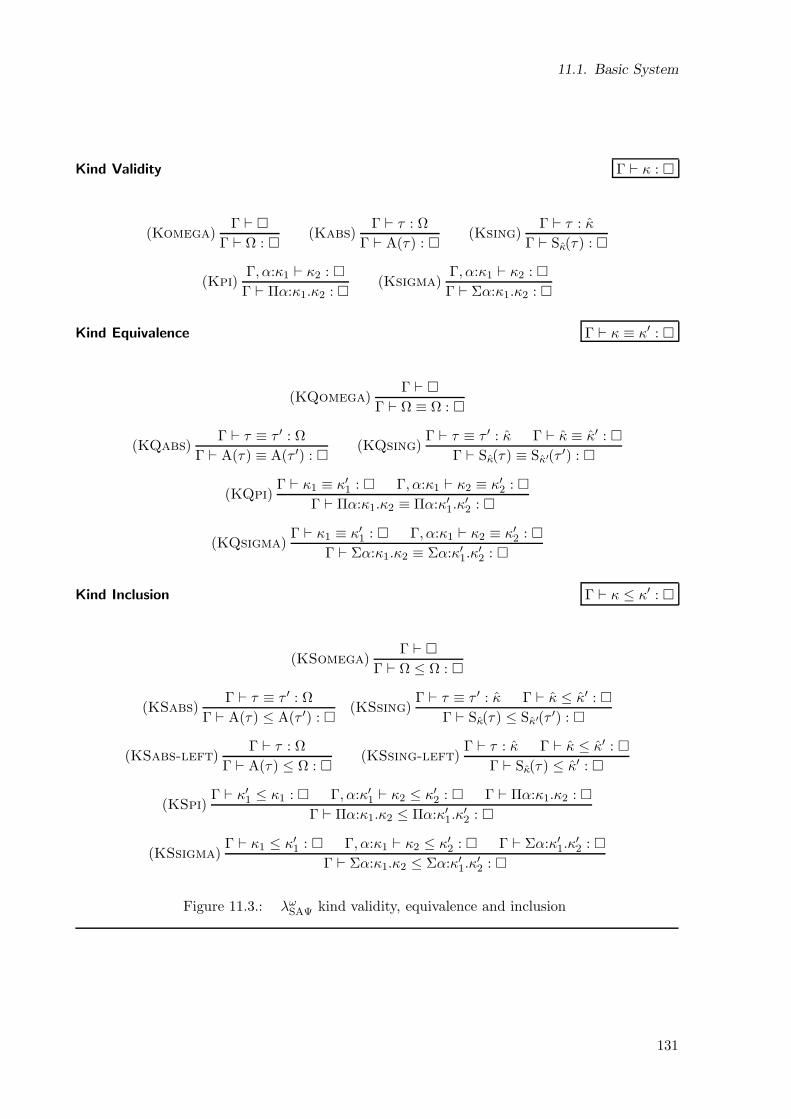
11.1. Basic System
Kind Validity Γ ⊢ κ :
(Komega)Γ ⊢
Γ ⊢ Ω : (Kabs)
Γ ⊢ τ : Ω
Γ ⊢ A(τ) : (Ksing)
Γ ⊢ τ : κ
Γ ⊢ Sκ(τ) :
(Kpi)Γ, α:κ1 ⊢ κ2 :
Γ ⊢ Πα:κ1.κ2 : (Ksigma)
Γ, α:κ1 ⊢ κ2 :
Γ ⊢ Σα:κ1.κ2 :
Kind Equivalence Γ ⊢ κ ≡ κ′ :
(KQomega)Γ ⊢
Γ ⊢ Ω ≡ Ω :
(KQabs)Γ ⊢ τ ≡ τ ′ : Ω
Γ ⊢ A(τ) ≡ A(τ ′) : (KQsing)
Γ ⊢ τ ≡ τ ′ : κ Γ ⊢ κ ≡ κ′ :
Γ ⊢ Sκ(τ) ≡ Sκ′(τ ′) :
(KQpi)Γ ⊢ κ1 ≡ κ′1 : Γ, α:κ1 ⊢ κ2 ≡ κ′2 :
Γ ⊢ Πα:κ1.κ2 ≡ Πα:κ′1.κ′2 :
(KQsigma)Γ ⊢ κ1 ≡ κ′1 : Γ, α:κ1 ⊢ κ2 ≡ κ′2 :
Γ ⊢ Σα:κ1.κ2 ≡ Σα:κ′1.κ′2 :
Kind Inclusion Γ ⊢ κ ≤ κ′ :
(KSomega)Γ ⊢
Γ ⊢ Ω ≤ Ω :
(KSabs)Γ ⊢ τ ≡ τ ′ : Ω
Γ ⊢ A(τ) ≤ A(τ ′) : (KSsing)
Γ ⊢ τ ≡ τ ′ : κ Γ ⊢ κ ≤ κ′ :
Γ ⊢ Sκ(τ) ≤ Sκ′(τ ′) :
(KSabs-left)Γ ⊢ τ : Ω
Γ ⊢ A(τ) ≤ Ω : (KSsing-left)
Γ ⊢ τ : κ Γ ⊢ κ ≤ κ′ :
Γ ⊢ Sκ(τ) ≤ κ′ :
(KSpi)Γ ⊢ κ′1 ≤ κ1 : Γ, α:κ′1 ⊢ κ2 ≤ κ′2 : Γ ⊢ Πα:κ1.κ2 :
Γ ⊢ Πα:κ1.κ2 ≤ Πα:κ′1.κ′2 :
(KSsigma)Γ ⊢ κ1 ≤ κ′1 : Γ, α:κ1 ⊢ κ2 ≤ κ′2 : Γ ⊢ Σα:κ′1.κ
′2 :
Γ ⊢ Σα:κ1.κ2 ≤ Σα:κ′1.κ′2 :
Figure 11.3.: λωSAΨ kind validity, equivalence and inclusion
131
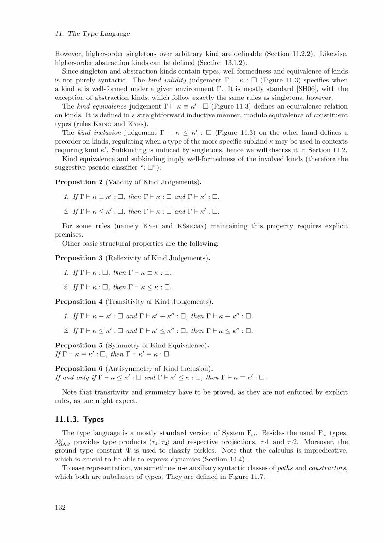
11. The Type Language
However, higher-order singletons over arbitrary kind are definable (Section 11.2.2). Likewise,higher-order abstraction kinds can be defined (Section 13.1.2).
Since singleton and abstraction kinds contain types, well-formedness and equivalence of kindsis not purely syntactic. The kind validity judgement Γ ⊢ κ : (Figure 11.3) specifies whena kind κ is well-formed under a given environment Γ. It is mostly standard [SH06], with theexception of abstraction kinds, which follow exactly the same rules as singletons, however.
The kind equivalence judgement Γ ⊢ κ ≡ κ′ : (Figure 11.3) defines an equivalence relationon kinds. It is defined in a straightforward inductive manner, modulo equivalence of constituenttypes (rules Ksing and Kabs).
The kind inclusion judgement Γ ⊢ κ ≤ κ′ : (Figure 11.3) on the other hand defines apreorder on kinds, regulating when a type of the more specific subkind κ may be used in contextsrequiring kind κ′. Subkinding is induced by singletons, hence we will discuss it in Section 11.2.
Kind equivalence and subkinding imply well-formedness of the involved kinds (therefore thesuggestive pseudo classifier “: ”):
Proposition 2 (Validity of Kind Judgements).
1. If Γ ⊢ κ ≡ κ′ : , then Γ ⊢ κ : and Γ ⊢ κ′ : .
2. If Γ ⊢ κ ≤ κ′ : , then Γ ⊢ κ : and Γ ⊢ κ′ : .
For some rules (namely KSpi and KSsigma) maintaining this property requires explicitpremises.
Other basic structural properties are the following:
Proposition 3 (Reflexivity of Kind Judgements).
1. If Γ ⊢ κ : , then Γ ⊢ κ ≡ κ : .
2. If Γ ⊢ κ : , then Γ ⊢ κ ≤ κ : .
Proposition 4 (Transitivity of Kind Judgements).
1. If Γ ⊢ κ ≡ κ′ : and Γ ⊢ κ′ ≡ κ′′ : , then Γ ⊢ κ ≡ κ′′ : .
2. If Γ ⊢ κ ≤ κ′ : and Γ ⊢ κ′ ≤ κ′′ : , then Γ ⊢ κ ≤ κ′′ : .
Proposition 5 (Symmetry of Kind Equivalence).If Γ ⊢ κ ≡ κ′ : , then Γ ⊢ κ′ ≡ κ : .
Proposition 6 (Antisymmetry of Kind Inclusion).If and only if Γ ⊢ κ ≤ κ′ : and Γ ⊢ κ′ ≤ κ : , then Γ ⊢ κ ≡ κ′ : .
Note that transitivity and symmetry have to be proved, as they are not enforced by explicitrules, as one might expect.
11.1.3. Types
The type language is a mostly standard version of System Fω. Besides the usual Fω types,λω
SAΨ provides type products 〈τ1, τ2〉 and respective projections, τ ·1 and τ ·2. Moreover, theground type constant Ψ is used to classify pickles. Note that the calculus is impredicative,which is crucial to be able to express dynamics (Section 10.4).
To ease representation, we sometimes use auxiliary syntactic classes of paths and constructors,which both are subclasses of types. They are defined in Figure 11.7.
132
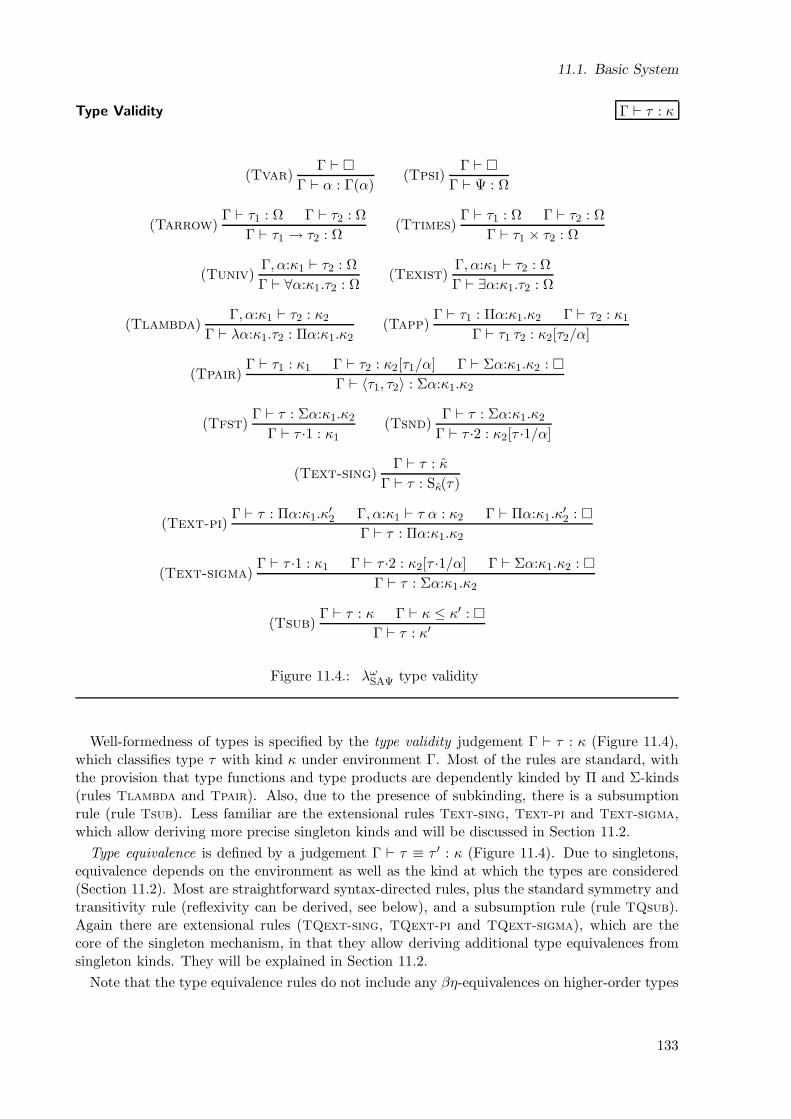
11.1. Basic System
Type Validity Γ ⊢ τ : κ
(Tvar)Γ ⊢
Γ ⊢ α : Γ(α)(Tpsi)
Γ ⊢
Γ ⊢ Ψ : Ω
(Tarrow)Γ ⊢ τ1 : Ω Γ ⊢ τ2 : Ω
Γ ⊢ τ1 → τ2 : Ω(Ttimes)
Γ ⊢ τ1 : Ω Γ ⊢ τ2 : Ω
Γ ⊢ τ1 × τ2 : Ω
(Tuniv)Γ, α:κ1 ⊢ τ2 : Ω
Γ ⊢ ∀α:κ1.τ2 : Ω(Texist)
Γ, α:κ1 ⊢ τ2 : Ω
Γ ⊢ ∃α:κ1.τ2 : Ω
(Tlambda)Γ, α:κ1 ⊢ τ2 : κ2
Γ ⊢ λα:κ1.τ2 : Πα:κ1.κ2(Tapp)
Γ ⊢ τ1 : Πα:κ1.κ2 Γ ⊢ τ2 : κ1
Γ ⊢ τ1 τ2 : κ2[τ2/α]
(Tpair)Γ ⊢ τ1 : κ1 Γ ⊢ τ2 : κ2[τ1/α] Γ ⊢ Σα:κ1.κ2 :
Γ ⊢ 〈τ1, τ2〉 : Σα:κ1.κ2
(Tfst)Γ ⊢ τ : Σα:κ1.κ2
Γ ⊢ τ ·1 : κ1(Tsnd)
Γ ⊢ τ : Σα:κ1.κ2
Γ ⊢ τ ·2 : κ2[τ ·1/α]
(Text-sing)Γ ⊢ τ : κ
Γ ⊢ τ : Sκ(τ)
(Text-pi)Γ ⊢ τ : Πα:κ1.κ
′2 Γ, α:κ1 ⊢ τ α : κ2 Γ ⊢ Πα:κ1.κ
′2 :
Γ ⊢ τ : Πα:κ1.κ2
(Text-sigma)Γ ⊢ τ ·1 : κ1 Γ ⊢ τ ·2 : κ2[τ ·1/α] Γ ⊢ Σα:κ1.κ2 :
Γ ⊢ τ : Σα:κ1.κ2
(Tsub)Γ ⊢ τ : κ Γ ⊢ κ ≤ κ′ :
Γ ⊢ τ : κ′
Figure 11.4.: λωSAΨ type validity
Well-formedness of types is specified by the type validity judgement Γ ⊢ τ : κ (Figure 11.4),which classifies type τ with kind κ under environment Γ. Most of the rules are standard, withthe provision that type functions and type products are dependently kinded by Π and Σ-kinds(rules Tlambda and Tpair). Also, due to the presence of subkinding, there is a subsumptionrule (rule Tsub). Less familiar are the extensional rules Text-sing, Text-pi and Text-sigma,which allow deriving more precise singleton kinds and will be discussed in Section 11.2.
Type equivalence is defined by a judgement Γ ⊢ τ ≡ τ ′ : κ (Figure 11.4). Due to singletons,equivalence depends on the environment as well as the kind at which the types are considered(Section 11.2). Most are straightforward syntax-directed rules, plus the standard symmetry andtransitivity rule (reflexivity can be derived, see below), and a subsumption rule (rule TQsub).Again there are extensional rules (TQext-sing, TQext-pi and TQext-sigma), which are thecore of the singleton mechanism, in that they allow deriving additional type equivalences fromsingleton kinds. They will be explained in Section 11.2.
Note that the type equivalence rules do not include any βη-equivalences on higher-order types
133
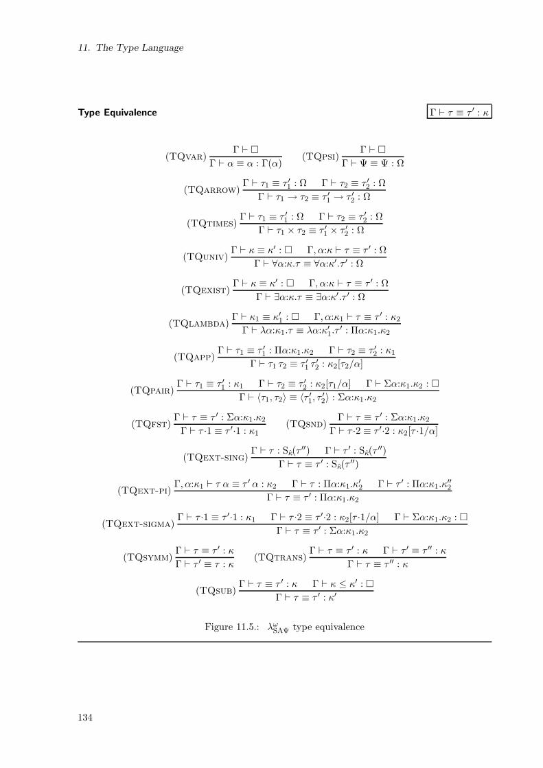
11. The Type Language
Type Equivalence Γ ⊢ τ ≡ τ ′ : κ
(TQvar)Γ ⊢
Γ ⊢ α ≡ α : Γ(α)(TQpsi)
Γ ⊢
Γ ⊢ Ψ ≡ Ψ : Ω
(TQarrow)Γ ⊢ τ1 ≡ τ ′1 : Ω Γ ⊢ τ2 ≡ τ ′2 : Ω
Γ ⊢ τ1 → τ2 ≡ τ ′1 → τ ′2 : Ω
(TQtimes)Γ ⊢ τ1 ≡ τ ′1 : Ω Γ ⊢ τ2 ≡ τ ′2 : Ω
Γ ⊢ τ1 × τ2 ≡ τ ′1 × τ ′2 : Ω
(TQuniv)Γ ⊢ κ ≡ κ′ : Γ, α:κ ⊢ τ ≡ τ ′ : Ω
Γ ⊢ ∀α:κ.τ ≡ ∀α:κ′.τ ′ : Ω
(TQexist)Γ ⊢ κ ≡ κ′ : Γ, α:κ ⊢ τ ≡ τ ′ : Ω
Γ ⊢ ∃α:κ.τ ≡ ∃α:κ′.τ ′ : Ω
(TQlambda)Γ ⊢ κ1 ≡ κ′1 : Γ, α:κ1 ⊢ τ ≡ τ ′ : κ2
Γ ⊢ λα:κ1.τ ≡ λα:κ′1.τ′ : Πα:κ1.κ2
(TQapp)Γ ⊢ τ1 ≡ τ ′1 : Πα:κ1.κ2 Γ ⊢ τ2 ≡ τ ′2 : κ1
Γ ⊢ τ1 τ2 ≡ τ ′1 τ′2 : κ2[τ2/α]
(TQpair)Γ ⊢ τ1 ≡ τ ′1 : κ1 Γ ⊢ τ2 ≡ τ ′2 : κ2[τ1/α] Γ ⊢ Σα:κ1.κ2 :
Γ ⊢ 〈τ1, τ2〉 ≡ 〈τ ′1, τ′2〉 : Σα:κ1.κ2
(TQfst)Γ ⊢ τ ≡ τ ′ : Σα:κ1.κ2
Γ ⊢ τ ·1 ≡ τ ′·1 : κ1(TQsnd)
Γ ⊢ τ ≡ τ ′ : Σα:κ1.κ2
Γ ⊢ τ ·2 ≡ τ ′·2 : κ2[τ ·1/α]
(TQext-sing)Γ ⊢ τ : Sκ(τ
′′) Γ ⊢ τ ′ : Sκ(τ′′)
Γ ⊢ τ ≡ τ ′ : Sκ(τ′′)
(TQext-pi)Γ, α:κ1 ⊢ τ α ≡ τ ′ α : κ2 Γ ⊢ τ : Πα:κ1.κ
′2 Γ ⊢ τ ′ : Πα:κ1.κ
′′2
Γ ⊢ τ ≡ τ ′ : Πα:κ1.κ2
(TQext-sigma)Γ ⊢ τ ·1 ≡ τ ′·1 : κ1 Γ ⊢ τ ·2 ≡ τ ′·2 : κ2[τ ·1/α] Γ ⊢ Σα:κ1.κ2 :
Γ ⊢ τ ≡ τ ′ : Σα:κ1.κ2
(TQsymm)Γ ⊢ τ ≡ τ ′ : κ
Γ ⊢ τ ′ ≡ τ : κ(TQtrans)
Γ ⊢ τ ≡ τ ′ : κ Γ ⊢ τ ′ ≡ τ ′′ : κ
Γ ⊢ τ ≡ τ ′′ : κ
(TQsub)Γ ⊢ τ ≡ τ ′ : κ Γ ⊢ κ ≤ κ′ :
Γ ⊢ τ ≡ τ ′ : κ′
Figure 11.5.: λωSAΨ type equivalence
134
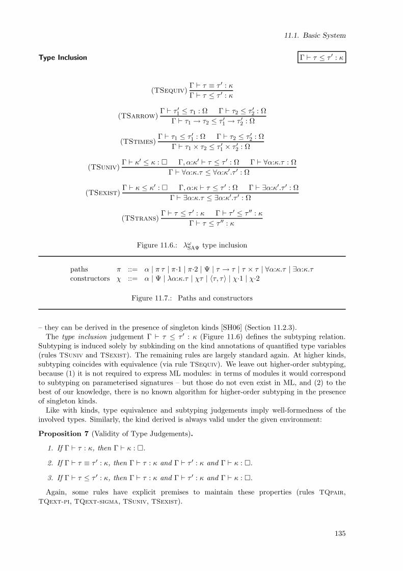
11.1. Basic System
Type Inclusion Γ ⊢ τ ≤ τ ′ : κ
(TSequiv)Γ ⊢ τ ≡ τ ′ : κ
Γ ⊢ τ ≤ τ ′ : κ
(TSarrow)Γ ⊢ τ ′1 ≤ τ1 : Ω Γ ⊢ τ2 ≤ τ ′2 : Ω
Γ ⊢ τ1 → τ2 ≤ τ ′1 → τ ′2 : Ω
(TStimes)Γ ⊢ τ1 ≤ τ ′1 : Ω Γ ⊢ τ2 ≤ τ ′2 : Ω
Γ ⊢ τ1 × τ2 ≤ τ ′1 × τ ′2 : Ω
(TSuniv)Γ ⊢ κ′ ≤ κ : Γ, α:κ′ ⊢ τ ≤ τ ′ : Ω Γ ⊢ ∀α:κ.τ : Ω
Γ ⊢ ∀α:κ.τ ≤ ∀α:κ′.τ ′ : Ω
(TSexist)Γ ⊢ κ ≤ κ′ : Γ, α:κ ⊢ τ ≤ τ ′ : Ω Γ ⊢ ∃α:κ′.τ ′ : Ω
Γ ⊢ ∃α:κ.τ ≤ ∃α:κ′.τ ′ : Ω
(TStrans)Γ ⊢ τ ≤ τ ′ : κ Γ ⊢ τ ′ ≤ τ ′′ : κ
Γ ⊢ τ ≤ τ ′′ : κ
Figure 11.6.: λωSAΨ type inclusion
paths π ::= α | π τ | π·1 | π·2 | Ψ | τ → τ | τ × τ | ∀α:κ.τ | ∃α:κ.τconstructors χ ::= α | Ψ | λα:κ.τ | χτ | 〈τ, τ〉 | χ·1 | χ·2
Figure 11.7.: Paths and constructors
– they can be derived in the presence of singleton kinds [SH06] (Section 11.2.3).The type inclusion judgement Γ ⊢ τ ≤ τ ′ : κ (Figure 11.6) defines the subtyping relation.
Subtyping is induced solely by subkinding on the kind annotations of quantified type variables(rules TSuniv and TSexist). The remaining rules are largely standard again. At higher kinds,subtyping coincides with equivalence (via rule TSequiv). We leave out higher-order subtyping,because (1) it is not required to express ML modules: in terms of modules it would correspondto subtyping on parameterised signatures – but those do not even exist in ML, and (2) to thebest of our knowledge, there is no known algorithm for higher-order subtyping in the presenceof singleton kinds.
Like with kinds, type equivalence and subtyping judgements imply well-formedness of theinvolved types. Similarly, the kind derived is always valid under the given environment:
Proposition 7 (Validity of Type Judgements).
1. If Γ ⊢ τ : κ, then Γ ⊢ κ : .
2. If Γ ⊢ τ ≡ τ ′ : κ, then Γ ⊢ τ : κ and Γ ⊢ τ ′ : κ and Γ ⊢ κ : .
3. If Γ ⊢ τ ≤ τ ′ : κ, then Γ ⊢ τ : κ and Γ ⊢ τ ′ : κ and Γ ⊢ κ : .
Again, some rules have explicit premises to maintain these properties (rules TQpair,TQext-pi, TQext-sigma, TSuniv, TSexist).
135
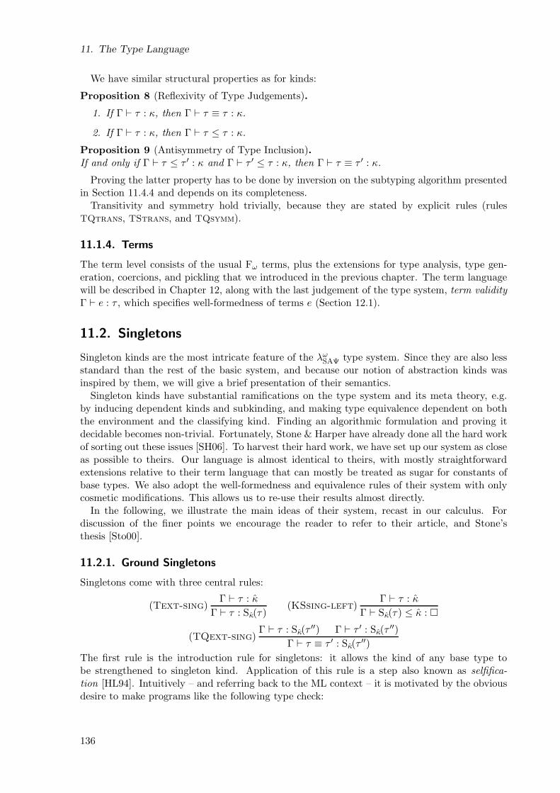
11. The Type Language
We have similar structural properties as for kinds:
Proposition 8 (Reflexivity of Type Judgements).
1. If Γ ⊢ τ : κ, then Γ ⊢ τ ≡ τ : κ.
2. If Γ ⊢ τ : κ, then Γ ⊢ τ ≤ τ : κ.
Proposition 9 (Antisymmetry of Type Inclusion).If and only if Γ ⊢ τ ≤ τ ′ : κ and Γ ⊢ τ ′ ≤ τ : κ, then Γ ⊢ τ ≡ τ ′ : κ.
Proving the latter property has to be done by inversion on the subtyping algorithm presentedin Section 11.4.4 and depends on its completeness.
Transitivity and symmetry hold trivially, because they are stated by explicit rules (rulesTQtrans, TStrans, and TQsymm).
11.1.4. Terms
The term level consists of the usual Fω terms, plus the extensions for type analysis, type gen-eration, coercions, and pickling that we introduced in the previous chapter. The term languagewill be described in Chapter 12, along with the last judgement of the type system, term validityΓ ⊢ e : τ , which specifies well-formedness of terms e (Section 12.1).
11.2. Singletons
Singleton kinds are the most intricate feature of the λωSAΨ type system. Since they are also less
standard than the rest of the basic system, and because our notion of abstraction kinds wasinspired by them, we will give a brief presentation of their semantics.
Singleton kinds have substantial ramifications on the type system and its meta theory, e.g.by inducing dependent kinds and subkinding, and making type equivalence dependent on boththe environment and the classifying kind. Finding an algorithmic formulation and proving itdecidable becomes non-trivial. Fortunately, Stone & Harper have already done all the hard workof sorting out these issues [SH06]. To harvest their hard work, we have set up our system as closeas possible to theirs. Our language is almost identical to theirs, with mostly straightforwardextensions relative to their term language that can mostly be treated as sugar for constants ofbase types. We also adopt the well-formedness and equivalence rules of their system with onlycosmetic modifications. This allows us to re-use their results almost directly.
In the following, we illustrate the main ideas of their system, recast in our calculus. Fordiscussion of the finer points we encourage the reader to refer to their article, and Stone’sthesis [Sto00].
11.2.1. Ground Singletons
Singletons come with three central rules:
(Text-sing)Γ ⊢ τ : κ
Γ ⊢ τ : Sκ(τ)(KSsing-left)
Γ ⊢ τ : κ
Γ ⊢ Sκ(τ) ≤ κ :
(TQext-sing)Γ ⊢ τ : Sκ(τ
′′) Γ ⊢ τ ′ : Sκ(τ′′)
Γ ⊢ τ ≡ τ ′ : Sκ(τ′′)
The first rule is the introduction rule for singletons: it allows the kind of any base type tobe strengthened to singleton kind. Application of this rule is a step also known as selfifica-tion [HL94]. Intuitively – and referring back to the ML context – it is motivated by the obviousdesire to make programs like the following type check:
136
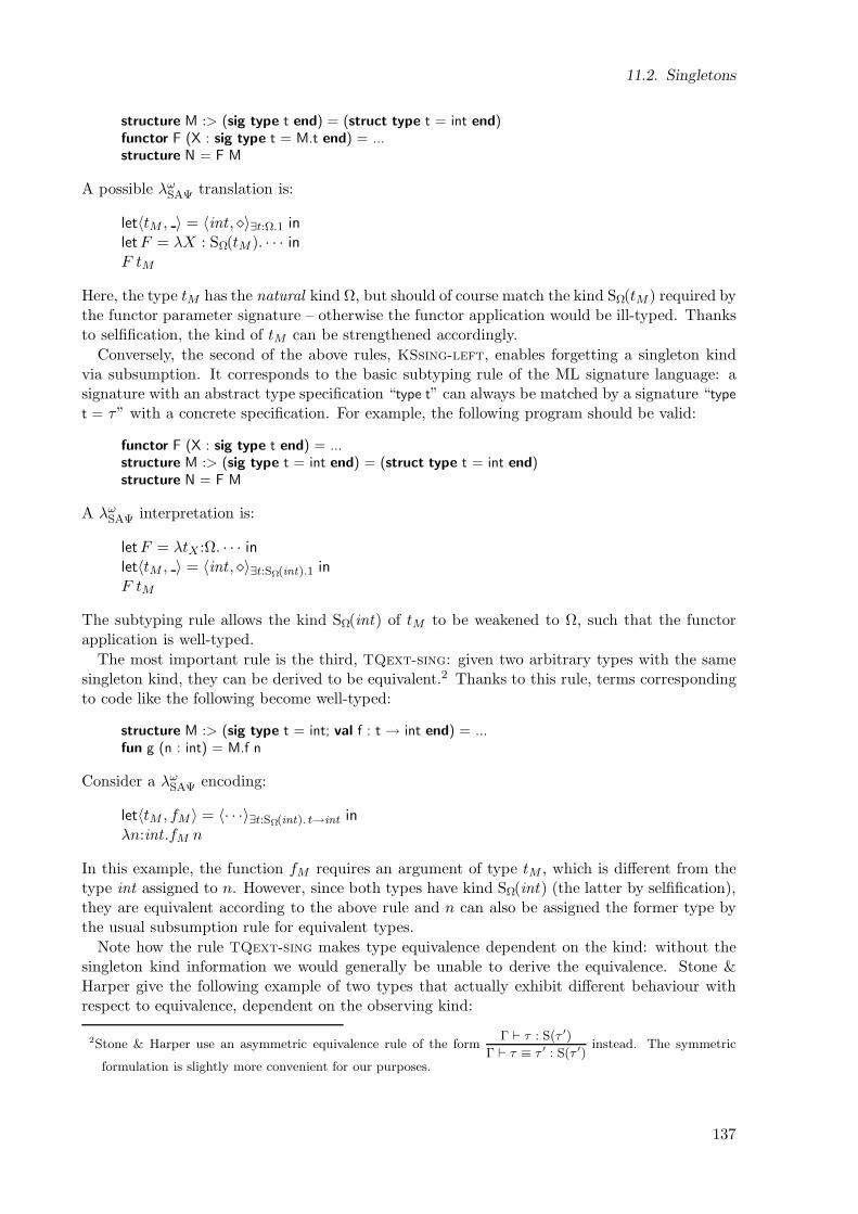
11.2. Singletons
structure M :> (sig type t end) = (struct type t = int end)functor F (X : sig type t = M.t end) = ...structure N = F M
A possible λωSAΨ translation is:
let〈tM , 〉 = 〈int , ⋄〉∃t:Ω.1 inletF = λX : SΩ(tM ). · · · inF tM
Here, the type tM has the natural kind Ω, but should of course match the kind SΩ(tM ) required bythe functor parameter signature – otherwise the functor application would be ill-typed. Thanksto selfification, the kind of tM can be strengthened accordingly.
Conversely, the second of the above rules, KSsing-left, enables forgetting a singleton kindvia subsumption. It corresponds to the basic subtyping rule of the ML signature language: asignature with an abstract type specification “type t” can always be matched by a signature “type
t = τ” with a concrete specification. For example, the following program should be valid:
functor F (X : sig type t end) = ...structure M :> (sig type t = int end) = (struct type t = int end)structure N = F M
A λωSAΨ interpretation is:
letF = λtX :Ω. · · · inlet〈tM , 〉 = 〈int , ⋄〉∃t:SΩ(int).1 inF tM
The subtyping rule allows the kind SΩ(int) of tM to be weakened to Ω, such that the functorapplication is well-typed.
The most important rule is the third, TQext-sing: given two arbitrary types with the samesingleton kind, they can be derived to be equivalent.2 Thanks to this rule, terms correspondingto code like the following become well-typed:
structure M :> (sig type t = int; val f : t → int end) = ...fun g (n : int) = M.f n
Consider a λωSAΨ encoding:
let〈tM , fM 〉 = 〈· · ·〉∃t:SΩ(int). t→int inλn:int .fM n
In this example, the function fM requires an argument of type tM , which is different from thetype int assigned to n. However, since both types have kind SΩ(int) (the latter by selfification),they are equivalent according to the above rule and n can also be assigned the former type bythe usual subsumption rule for equivalent types.
Note how the rule TQext-sing makes type equivalence dependent on the kind: without thesingleton kind information we would generally be unable to derive the equivalence. Stone &Harper give the following example of two types that actually exhibit different behaviour withrespect to equivalence, dependent on the observing kind:
2Stone & Harper use an asymmetric equivalence rule of the formΓ ⊢ τ : S(τ ′)
Γ ⊢ τ ≡ τ′ : S(τ ′)
instead. The symmetric
formulation is slightly more convenient for our purposes.
137
11. The Type Language
S(τ : Ω) := SΩ(τ)S(τ : A(τ ′)) := SA(τ ′)(τ)
S(τ : Sκ(τ′)) := Sκ(τ
′)S(τ : Πα:κ1.κ2) := Πα:κ1.S(τ α : κ2)S(τ : Σα:κ1.κ2) := S(τ ·1 : κ1) × S(τ ·2 : κ2[τ ·1/α])
Figure 11.8.: Higher-order singletons
τ1 = λα:Ω.ατ2 = λα:Ω.int
Both these types can be assigned kind Πα:Ω.Ω, under which they clearly differ. However, bysubsumption both also can be given the contravariant superkind Πα:SΩ(int).Ω, under whichthey are equivalent, because the only valid argument is type int , for which they both deliver thesame result!
11.2.2. Higher-Order Singletons
Singleton kinds are only defined on types of base kind. What about higher-order types? Forexample, how can the following ML signature be expressed?
sig type α pair = α × α end
The specification for type pair would correspond to a singleton S(λα:Ω.α×α). The kind of thecontained type function is Ω → Ω, however (i.e. Πα:Ω.Ω). Thus we need singletons at higher-order kind to express it.
Fortunately, it is not necessary to introduce higher-order singletons as primitive – they can bedefined inductively as syntactic sugar. Figure 11.8 gives a respective definition following Stone& Harper [SH06]. The only exception are abstraction kinds, which require primitive support(Section 11.3.1).
Higher-order singletons are defined such that generalised versions of the singleton rules pre-sented previously can be shown as propositions. These rules are given in Figure 11.9. Here andelsewhere, we will use the convention to name derived rules by appending an asterisk *.
Theorem 10 (Admissibility of Higher-Order Singleton Rules).The rules Ksing*, Text-sing, KQsing*, KSsing*, KSsing-left* and TQext-sing* are deriv-able.
Establishing the admissibility proofs crucially relies on extensional validity and equiva-lence rules for higher-order kinds that we have not discussed yet. Namely, the kinding rulesText-pi and Text-sigma (Figure 11.4) allow singleton kind selfification to be pushed throughη-expansions. For example, given Γ = α:(Σα1:Ω.Ω), rule Text-sigma enables deriving the mostprecise kind Γ ⊢ α : SΩ(α·1)× SΩ(α·2). Analogously, with the extensional rule Text-pi, we canderive β:(Πα1:Ω.Ω) ⊢ β : Πα1:Ω.SΩ(t α1), which indicates the kind of a type function that alwaysdeliver the same result as β – hence this is exactly the definition of a higher-order singleton atΠ-kind, i.e. we have derived Γ ⊢ β : S(β : Ω → Ω).
Similar extensionality rules are necessary for the type equivalence relation (Figure 11.5): ruleTQext-pi says that two type functions can be considered equivalent (under a given kind) whenthey deliver the same result for every argument (of the given argument kind). Likewise, ruleTQext-sigma says that pairs are equivalent whenever both their projections are.
138
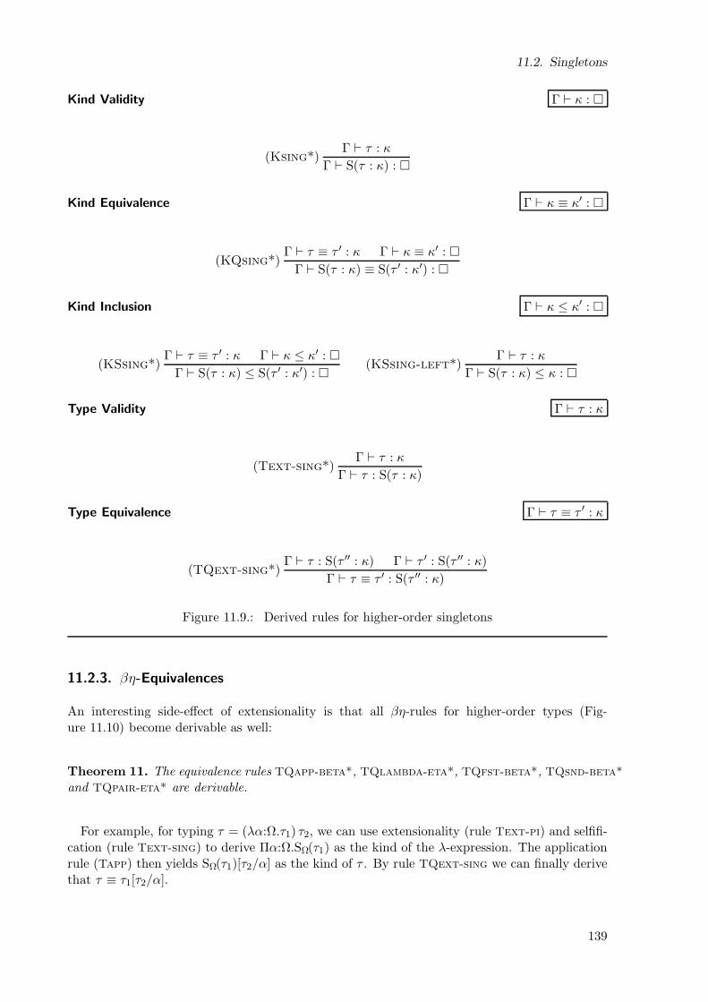
11.2. Singletons
Kind Validity Γ ⊢ κ :
(Ksing*)Γ ⊢ τ : κ
Γ ⊢ S(τ : κ) :
Kind Equivalence Γ ⊢ κ ≡ κ′ :
(KQsing*)Γ ⊢ τ ≡ τ ′ : κ Γ ⊢ κ ≡ κ′ :
Γ ⊢ S(τ : κ) ≡ S(τ ′ : κ′) :
Kind Inclusion Γ ⊢ κ ≤ κ′ :
(KSsing*)Γ ⊢ τ ≡ τ ′ : κ Γ ⊢ κ ≤ κ′ :
Γ ⊢ S(τ : κ) ≤ S(τ ′ : κ′) : (KSsing-left*)
Γ ⊢ τ : κ
Γ ⊢ S(τ : κ) ≤ κ :
Type Validity Γ ⊢ τ : κ
(Text-sing*)Γ ⊢ τ : κ
Γ ⊢ τ : S(τ : κ)
Type Equivalence Γ ⊢ τ ≡ τ ′ : κ
(TQext-sing*)Γ ⊢ τ : S(τ ′′ : κ) Γ ⊢ τ ′ : S(τ ′′ : κ)
Γ ⊢ τ ≡ τ ′ : S(τ ′′ : κ)
Figure 11.9.: Derived rules for higher-order singletons
11.2.3. βη-Equivalences
An interesting side-effect of extensionality is that all βη-rules for higher-order types (Fig-ure 11.10) become derivable as well:
Theorem 11. The equivalence rules TQapp-beta*, TQlambda-eta*, TQfst-beta*, TQsnd-beta*
and TQpair-eta* are derivable.
For example, for typing τ = (λα:Ω.τ1) τ2, we can use extensionality (rule Text-pi) and selfifi-cation (rule Text-sing) to derive Πα:Ω.SΩ(τ1) as the kind of the λ-expression. The applicationrule (Tapp) then yields SΩ(τ1)[τ2/α] as the kind of τ . By rule TQext-sing we can finally derivethat τ ≡ τ1[τ2/α].
139
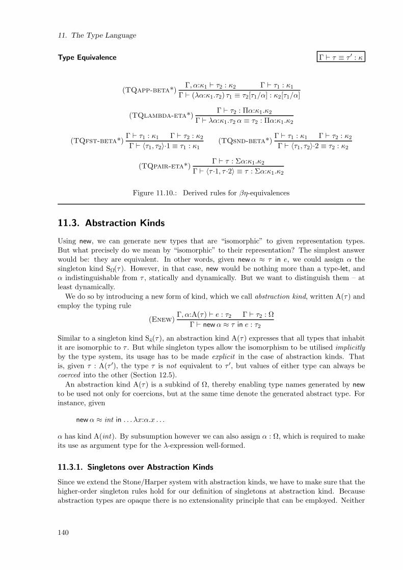
11. The Type Language
Type Equivalence Γ ⊢ τ ≡ τ ′ : κ
(TQapp-beta*)Γ, α:κ1 ⊢ τ2 : κ2 Γ ⊢ τ1 : κ1
Γ ⊢ (λα:κ1.τ2) τ1 ≡ τ2[τ1/α] : κ2[τ1/α]
(TQlambda-eta*)Γ ⊢ τ2 : Πα:κ1.κ2
Γ ⊢ λα:κ1.τ2 α ≡ τ2 : Πα:κ1.κ2
(TQfst-beta*)Γ ⊢ τ1 : κ1 Γ ⊢ τ2 : κ2
Γ ⊢ 〈τ1, τ2〉·1 ≡ τ1 : κ1(TQsnd-beta*)
Γ ⊢ τ1 : κ1 Γ ⊢ τ2 : κ2
Γ ⊢ 〈τ1, τ2〉·2 ≡ τ2 : κ2
(TQpair-eta*)Γ ⊢ τ : Σα:κ1.κ2
Γ ⊢ 〈τ ·1, τ ·2〉 ≡ τ : Σα:κ1.κ2
Figure 11.10.: Derived rules for βη-equivalences
11.3. Abstraction Kinds
Using new, we can generate new types that are “isomorphic” to given representation types.But what precisely do we mean by “isomorphic” to their representation? The simplest answerwould be: they are equivalent. In other words, given newα ≈ τ in e, we could assign α thesingleton kind SΩ(τ). However, in that case, new would be nothing more than a type-let, andα indistinguishable from τ , statically and dynamically. But we want to distinguish them – atleast dynamically.
We do so by introducing a new form of kind, which we call abstraction kind, written A(τ) andemploy the typing rule
(Enew)Γ, α:A(τ) ⊢ e : τ2 Γ ⊢ τ2 : Ω
Γ ⊢ newα ≈ τ in e : τ2
Similar to a singleton kind Sκ(τ), an abstraction kind A(τ) expresses that all types that inhabitit are isomorphic to τ . But while singleton types allow the isomorphism to be utilised implicitlyby the type system, its usage has to be made explicit in the case of abstraction kinds. Thatis, given τ : A(τ ′), the type τ is not equivalent to τ ′, but values of either type can always becoerced into the other (Section 12.5).
An abstraction kind A(τ) is a subkind of Ω, thereby enabling type names generated by newto be used not only for coercions, but at the same time denote the generated abstract type. Forinstance, given
newα ≈ int in . . . λx:α.x . . .
α has kind A(int). By subsumption however we can also assign α : Ω, which is required to makeits use as argument type for the λ-expression well-formed.
11.3.1. Singletons over Abstraction Kinds
Since we extend the Stone/Harper system with abstraction kinds, we have to make sure that thehigher-order singleton rules hold for our definition of singletons at abstraction kind. Becauseabstraction types are opaque there is no extensionality principle that can be employed. Neither
140
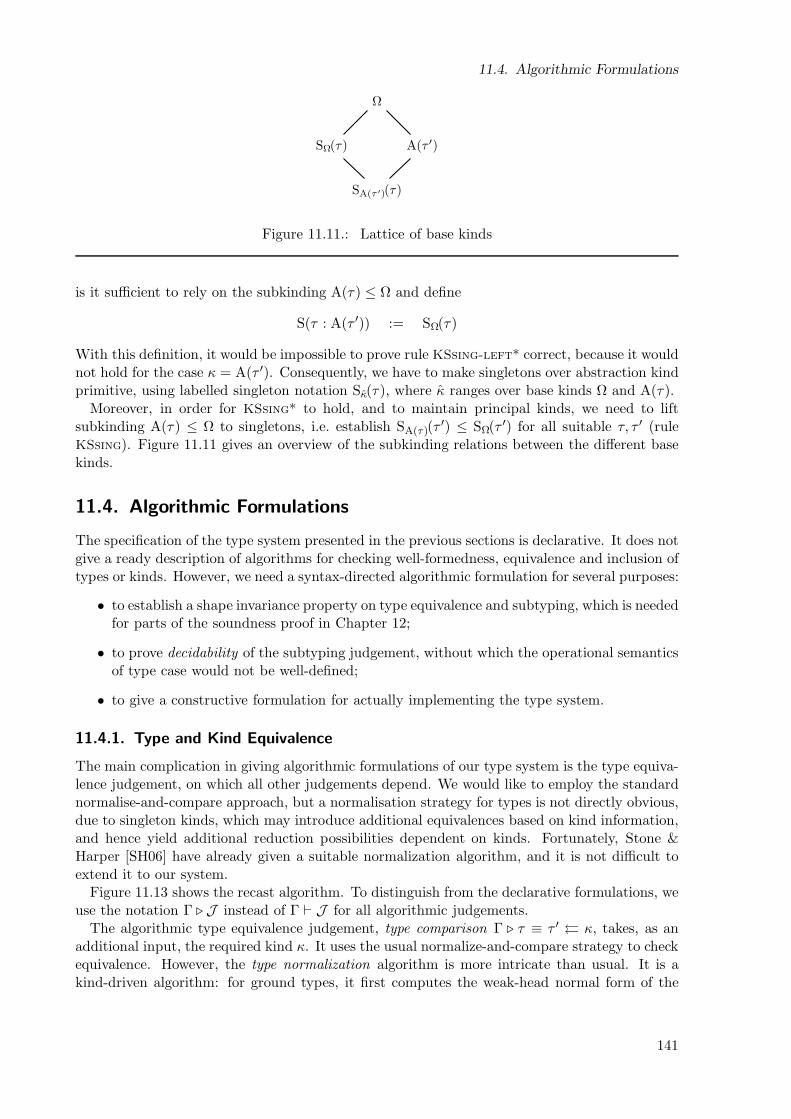
11.4. Algorithmic Formulations
Ω
SΩ(τ) A(τ ′)
SA(τ ′)(τ)
Figure 11.11.: Lattice of base kinds
is it sufficient to rely on the subkinding A(τ) ≤ Ω and define
S(τ : A(τ ′)) := SΩ(τ)
With this definition, it would be impossible to prove rule KSsing-left* correct, because it wouldnot hold for the case κ = A(τ ′). Consequently, we have to make singletons over abstraction kindprimitive, using labelled singleton notation Sκ(τ), where κ ranges over base kinds Ω and A(τ).
Moreover, in order for KSsing* to hold, and to maintain principal kinds, we need to liftsubkinding A(τ) ≤ Ω to singletons, i.e. establish SA(τ)(τ
′) ≤ SΩ(τ ′) for all suitable τ, τ ′ (ruleKSsing). Figure 11.11 gives an overview of the subkinding relations between the different basekinds.
11.4. Algorithmic Formulations
The specification of the type system presented in the previous sections is declarative. It does notgive a ready description of algorithms for checking well-formedness, equivalence and inclusion oftypes or kinds. However, we need a syntax-directed algorithmic formulation for several purposes:
• to establish a shape invariance property on type equivalence and subtyping, which is neededfor parts of the soundness proof in Chapter 12;
• to prove decidability of the subtyping judgement, without which the operational semanticsof type case would not be well-defined;
• to give a constructive formulation for actually implementing the type system.
11.4.1. Type and Kind Equivalence
The main complication in giving algorithmic formulations of our type system is the type equiva-lence judgement, on which all other judgements depend. We would like to employ the standardnormalise-and-compare approach, but a normalisation strategy for types is not directly obvious,due to singleton kinds, which may introduce additional equivalences based on kind information,and hence yield additional reduction possibilities dependent on kinds. Fortunately, Stone &Harper [SH06] have already given a suitable normalization algorithm, and it is not difficult toextend it to our system.
Figure 11.13 shows the recast algorithm. To distinguish from the declarative formulations, weuse the notation Γ ⊲ J instead of Γ ⊢ J for all algorithmic judgements.
The algorithmic type equivalence judgement, type comparison Γ ⊲ τ ≡ τ ′ κ, takes, as anadditional input, the required kind κ. It uses the usual normalize-and-compare strategy to checkequivalence. However, the type normalization algorithm is more intricate than usual. It is akind-driven algorithm: for ground types, it first computes the weak-head normal form of the
141
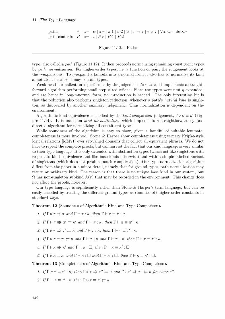
11. The Type Language
paths π ::= α | π τ | π·1 | π·2 | Ψ | τ → τ | τ × τ | ∀α:κ.τ | ∃α:κ.τpath contexts P ::= | P τ | P ·1 | P ·2
Figure 11.12.: Paths
type, also called a path (Figure 11.12). It then proceeds normalising remaining constituent typesby path normalization. For higher-order types, i.e. a function or pair, the judgement looks atthe η-expansions. To η-expand a lambda into a normal form it also has to normalize its kindannotation, because it may contain types.
Weak-head normalization is performed by the judgement Γ⊲τ π. It implements a straight-forward algorithm performing small step β-reductions. Since the types were first η-expanded,and are hence in long-η-normal form, no η-reduction is needed. The only interesting bit isthat the reduction also performs singleton reduction, whenever a path’s natural kind is single-ton, as discovered by another auxiliary judgement. Thus normalization is dependent on theenvironment.
Algorithmic kind equivalence is checked by the kind comparison judgement, Γ ⊲ κ ≡ κ′ (Fig-ure 11.14). It is based on kind normalization, which implements a straightforward syntax-directed algorithm for normalizing all constituent types.
While soundness of the algorithm is easy to show, given a handful of suitable lemmata,completeness is more involved. Stone & Harper show completeness using ternary Kripke-stylelogical relations [MM91] over set-valued domains that collect all equivalent phrases. We do nothave to repeat the complete proofs, but can harvest the fact that our kind language is very similarto their type language. It is only extended with abstraction types (which act like singletons withrespect to kind equivalence and like base kinds otherwise) and with a simple labelled variantof singletons (which does not produce much complication). Our type normalization algorithmdiffers from the paper in a minor detail, namely that for ground types, path normalization mayreturn an arbitrary kind. The reason is that there is no unique base kind in our system, butΩ has non-singleton subkind A(τ) that may be recorded in the environment. This change doesnot affect the proofs, however.
Our type language is significantly richer than Stone & Harper’s term language, but can beeasily encoded by treating the different ground types as (families of) higher-order constants instandard ways.
Theorem 12 (Soundness of Algorithmic Kind and Type Comparison).
1. If Γ ⊲ τ π and Γ ⊢ τ : κ, then Γ ⊢ τ ≡ π : κ.
2. If Γ ⊲ π π′ κ′ and Γ ⊢ π : κ, then Γ ⊢ π ≡ π′ : κ.
3. If Γ ⊲ τ τ ′ κ and Γ ⊢ τ : κ, then Γ ⊢ τ ≡ τ ′ : κ.
4. If Γ ⊲ τ ≡ τ ′ κ and Γ ⊢ τ : κ and Γ ⊢ τ ′ : κ, then Γ ⊢ τ ≡ τ ′ : κ.
5. If Γ ⊲ κ κ′ and Γ ⊢ κ : , then Γ ⊢ κ ≡ κ′ : .
6. If Γ ⊲ κ ≡ κ′ and Γ ⊢ κ : and Γ ⊢ κ′ : , then Γ ⊢ κ ≡ κ′ : .
Theorem 13 (Completeness of Algorithmic Kind and Type Comparison).
1. If Γ ⊢ τ ≡ τ ′ : κ, then Γ ⊲ τ τ ′′ κ and Γ ⊲ τ ′ τ ′′ κ for some τ ′′.
2. If Γ ⊢ τ ≡ τ ′ : κ, then Γ ⊲ τ ≡ τ ′ κ.
142
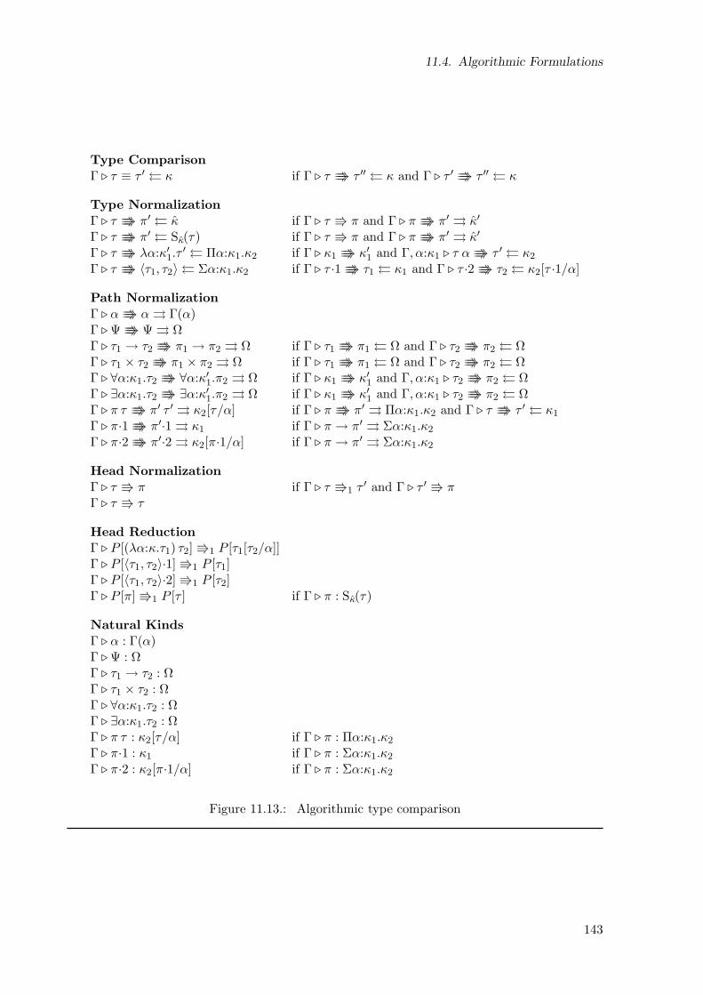
11.4. Algorithmic Formulations
Type Comparison
Γ ⊲ τ ≡ τ ′ κ if Γ ⊲ τ τ ′′ κ and Γ ⊲ τ ′ τ ′′ κ
Type Normalization
Γ ⊲ τ π′ κ if Γ ⊲ τ π and Γ ⊲ π π′ κ′
Γ ⊲ τ π′ Sκ(τ) if Γ ⊲ τ π and Γ ⊲ π π′ κ′
Γ ⊲ τ λα:κ′1.τ′ Πα:κ1.κ2 if Γ ⊲ κ1 κ′1 and Γ, α:κ1 ⊲ τ α τ ′ κ2
Γ ⊲ τ 〈τ1, τ2〉 Σα:κ1.κ2 if Γ ⊲ τ ·1 τ1 κ1 and Γ ⊲ τ ·2 τ2 κ2[τ ·1/α]
Path Normalization
Γ ⊲ α α Γ(α)Γ ⊲Ψ Ψ ΩΓ ⊲ τ1 → τ2 π1 → π2 Ω if Γ ⊲ τ1 π1 Ω and Γ ⊲ τ2 π2 ΩΓ ⊲ τ1 × τ2 π1 × π2 Ω if Γ ⊲ τ1 π1 Ω and Γ ⊲ τ2 π2 ΩΓ ⊲ ∀α:κ1.τ2 ∀α:κ′1.π2 Ω if Γ ⊲ κ1 κ′1 and Γ, α:κ1 ⊲ τ2 π2 ΩΓ ⊲ ∃α:κ1.τ2 ∃α:κ′1.π2 Ω if Γ ⊲ κ1 κ′1 and Γ, α:κ1 ⊲ τ2 π2 ΩΓ ⊲ π τ π′ τ ′ κ2[τ/α] if Γ ⊲ π π′ Πα:κ1.κ2 and Γ ⊲ τ τ ′ κ1
Γ ⊲ π·1 π′·1 κ1 if Γ ⊲ π → π′ Σα:κ1.κ2
Γ ⊲ π·2 π′·2 κ2[π·1/α] if Γ ⊲ π → π′ Σα:κ1.κ2
Head Normalization
Γ ⊲ τ π if Γ ⊲ τ 1 τ′ and Γ ⊲ τ ′ π
Γ ⊲ τ τ
Head Reduction
Γ ⊲ P [(λα:κ.τ1) τ2]1 P [τ1[τ2/α]]Γ ⊲ P [〈τ1, τ2〉·1]1 P [τ1]Γ ⊲ P [〈τ1, τ2〉·2]1 P [τ2]Γ ⊲ P [π]1 P [τ ] if Γ ⊲ π : Sκ(τ)
Natural Kinds
Γ ⊲ α : Γ(α)Γ ⊲Ψ : ΩΓ ⊲ τ1 → τ2 : ΩΓ ⊲ τ1 × τ2 : ΩΓ ⊲ ∀α:κ1.τ2 : ΩΓ ⊲ ∃α:κ1.τ2 : ΩΓ ⊲ π τ : κ2[τ/α] if Γ ⊲ π : Πα:κ1.κ2
Γ ⊲ π·1 : κ1 if Γ ⊲ π : Σα:κ1.κ2
Γ ⊲ π·2 : κ2[π·1/α] if Γ ⊲ π : Σα:κ1.κ2
Figure 11.13.: Algorithmic type comparison
143

11. The Type Language
Kind Comparison
Γ ⊲ κ ≡ κ′ if Γ ⊲ κ κ′′ and Γ ⊲ κ′ κ′′
Kind Normalization
Γ ⊲ Ω ΩΓ ⊲ A(τ) A(τ ′) if Γ ⊲ τ τ ′ ΩΓ ⊲ Sκ(τ) Sκ(τ
′) if Γ ⊲ τ τ ′ κΓ ⊲ Πα:κ1.κ2 Πα:κ′1.κ
′2 if Γ ⊲ κ1 κ′1 and Γ, α:κ1 ⊲ κ2 κ′2
Γ ⊲ Σα:κ1.κ2 Σα:κ′1.κ′2 if Γ ⊲ κ1 κ′1 and Γ, α:κ1 ⊲ κ2 κ′2
Figure 11.14.: Algorithmic kind comparison
Kind Matching
Γ ⊲ Ω ≤ ΩΓ ⊲ A(τ) ≤ ΩΓ ⊲ A(τ) ≤ A(τ ′) if Γ ⊲ τ ≡ τ ′ ΩΓ ⊲ Sκ(τ) ≤ κ′ if Γ ⊲ κ ≤ κ′
Γ ⊲ Sκ(τ) ≤ Sκ′(τ ′) if Γ ⊲ τ ≡ τ ′ κ and Γ ⊲ κ ≤ κ′
Γ ⊲ Πα:κ1.κ2 ≤ Πα:κ′1.κ′2 if Γ ⊲ κ′1 ≤ κ′1 and Γ, α:κ′1 ⊲ κ2 ≤ κ′2
Γ ⊲ Σα:κ1.κ2 ≤ Σα:κ′1.κ′2 if Γ ⊲ κ1 ≤ κ′1 and Γ, α:κ1 ⊲ κ2 ≤ κ′2
Figure 11.15.: Algorithmic kind matching
3. If Γ ⊢ κ ≡ κ′ : , then Γ ⊲ κ κ′′ and Γ ⊲ κ′ κ′′ for some κ′′.
4. If Γ ⊢ κ ≡ κ′ : , then Γ ⊲ κ ≡ κ′.
From soundness and completeness of the algorithmic equivalence judgements it follows imme-diately that the equivalence relations on kinds and types are decidable:
Corollary 14 (Decidability of Equivalence).
1. Given Γ ⊢ κ : and Γ ⊢ κ′ : , it is decidable whether Γ ⊢ κ ≡ κ : holds.
2. Given Γ ⊢ τ : κ and Γ ⊢ τ ′ : κ, it is decidable whether Γ ⊢ τ ≡ τ ′ : κ holds.
11.4.2. Subkinding
Given an algorithm for type equivalence, it is easy to define an algorithm to check subkinding.It is shown in Figure 11.15: kind checking, Γ ⊲ κ : , verifies that kind κ is well-formed underenvironment Γ, using straightforward structural recursion. The cases directly mirror the declar-ative rules. To check singletons and abstraction kinds, the algorithmic type equivalence checkis employed on the constituent types.
Theorem 15 (Soundness of Algorithmic Kind Matching).If Γ ⊲ κ ≤ κ′ and Γ ⊢ κ : and Γ ⊢ κ′ : , then Γ ⊢ κ ≤ κ′ : .
144
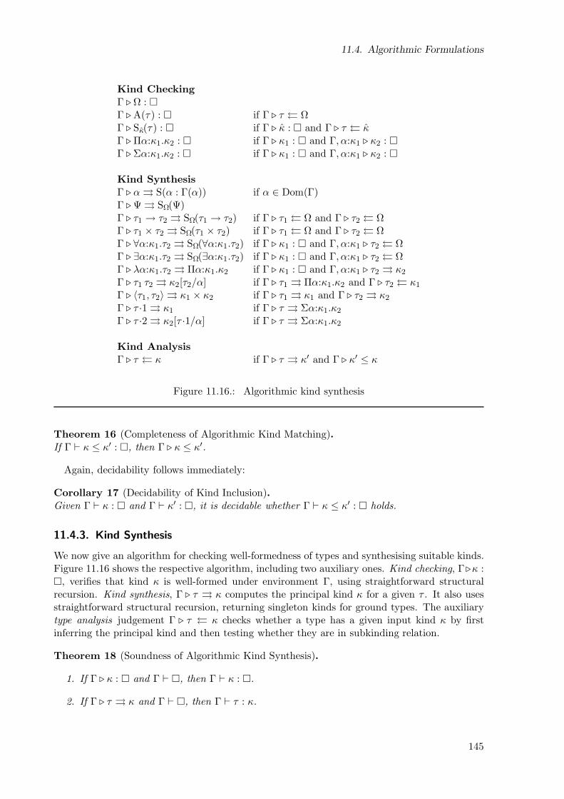
11.4. Algorithmic Formulations
Kind Checking
Γ ⊲Ω : Γ ⊲A(τ) : if Γ ⊲ τ ΩΓ ⊲ Sκ(τ) : if Γ ⊲ κ : and Γ ⊲ τ κΓ ⊲Πα:κ1.κ2 : if Γ ⊲ κ1 : and Γ, α:κ1 ⊲ κ2 : Γ ⊲Σα:κ1.κ2 : if Γ ⊲ κ1 : and Γ, α:κ1 ⊲ κ2 :
Kind Synthesis
Γ ⊲ α S(α : Γ(α)) if α ∈ Dom(Γ)Γ ⊲Ψ SΩ(Ψ)Γ ⊲ τ1 → τ2 SΩ(τ1 → τ2) if Γ ⊲ τ1 Ω and Γ ⊲ τ2 ΩΓ ⊲ τ1 × τ2 SΩ(τ1 × τ2) if Γ ⊲ τ1 Ω and Γ ⊲ τ2 ΩΓ ⊲ ∀α:κ1.τ2 SΩ(∀α:κ1.τ2) if Γ ⊲ κ1 : and Γ, α:κ1 ⊲ τ2 ΩΓ ⊲ ∃α:κ1.τ2 SΩ(∃α:κ1.τ2) if Γ ⊲ κ1 : and Γ, α:κ1 ⊲ τ2 ΩΓ ⊲ λα:κ1.τ2 Πα:κ1.κ2 if Γ ⊲ κ1 : and Γ, α:κ1 ⊲ τ2 κ2
Γ ⊲ τ1 τ2 κ2[τ2/α] if Γ ⊲ τ1 Πα:κ1.κ2 and Γ ⊲ τ2 κ1
Γ ⊲ 〈τ1, τ2〉 κ1 × κ2 if Γ ⊲ τ1 κ1 and Γ ⊲ τ2 κ2
Γ ⊲ τ ·1 κ1 if Γ ⊲ τ Σα:κ1.κ2
Γ ⊲ τ ·2 κ2[τ ·1/α] if Γ ⊲ τ Σα:κ1.κ2
Kind Analysis
Γ ⊲ τ κ if Γ ⊲ τ κ′ and Γ ⊲ κ′ ≤ κ
Figure 11.16.: Algorithmic kind synthesis
Theorem 16 (Completeness of Algorithmic Kind Matching).If Γ ⊢ κ ≤ κ′ : , then Γ ⊲ κ ≤ κ′.
Again, decidability follows immediately:
Corollary 17 (Decidability of Kind Inclusion).Given Γ ⊢ κ : and Γ ⊢ κ′ : , it is decidable whether Γ ⊢ κ ≤ κ′ : holds.
11.4.3. Kind Synthesis
We now give an algorithm for checking well-formedness of types and synthesising suitable kinds.Figure 11.16 shows the respective algorithm, including two auxiliary ones. Kind checking, Γ⊲κ :, verifies that kind κ is well-formed under environment Γ, using straightforward structuralrecursion. Kind synthesis, Γ ⊲ τ κ computes the principal kind κ for a given τ . It also usesstraightforward structural recursion, returning singleton kinds for ground types. The auxiliarytype analysis judgement Γ ⊲ τ κ checks whether a type has a given input kind κ by firstinferring the principal kind and then testing whether they are in subkinding relation.
Theorem 18 (Soundness of Algorithmic Kind Synthesis).
1. If Γ ⊲ κ : and Γ ⊢ , then Γ ⊢ κ : .
2. If Γ ⊲ τ κ and Γ ⊢ , then Γ ⊢ τ : κ.
145
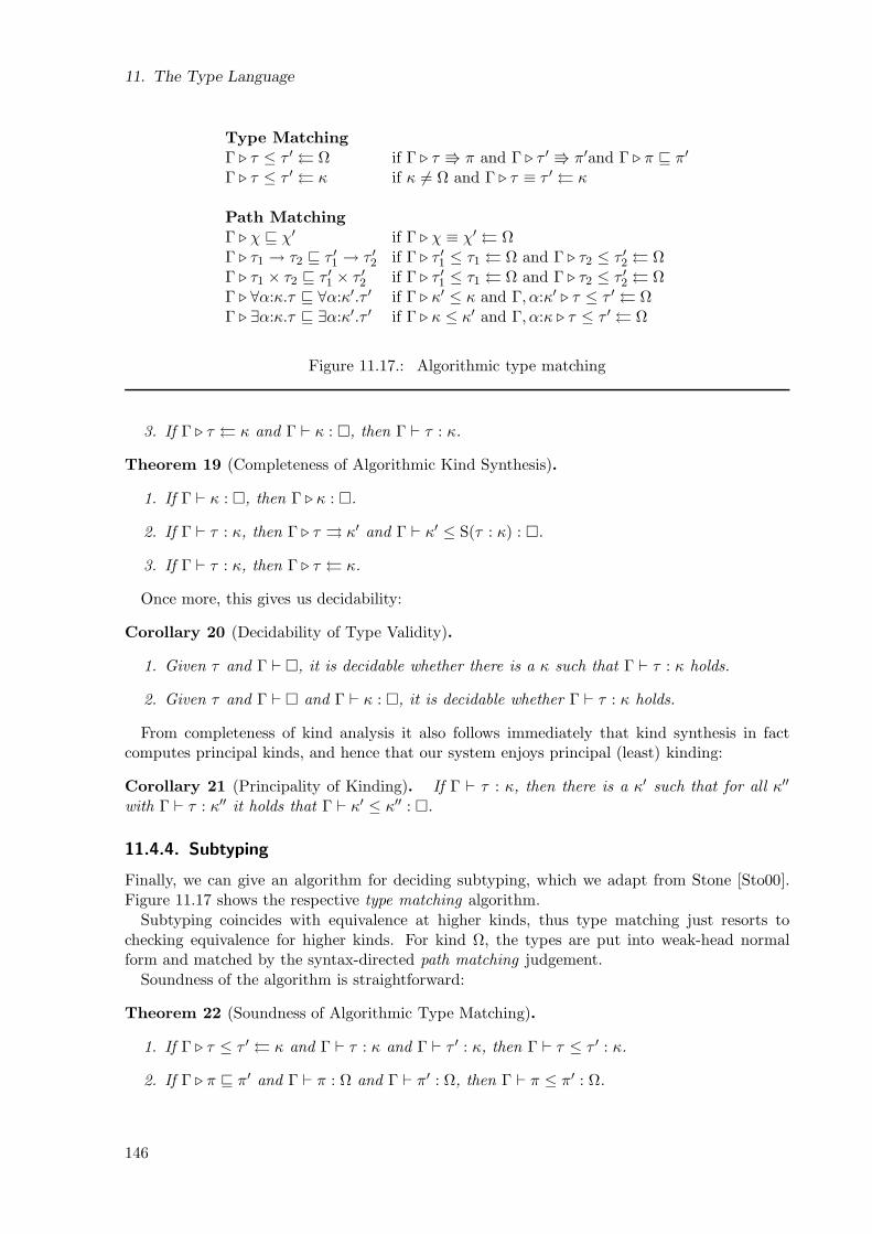
11. The Type Language
Type Matching
Γ ⊲ τ ≤ τ ′ Ω if Γ ⊲ τ π and Γ ⊲ τ ′ π′and Γ ⊲ π ⊑ π′
Γ ⊲ τ ≤ τ ′ κ if κ 6= Ω and Γ ⊲ τ ≡ τ ′ κ
Path Matching
Γ ⊲ χ ⊑ χ′ if Γ ⊲ χ ≡ χ′ ΩΓ ⊲ τ1 → τ2 ⊑ τ ′1 → τ ′2 if Γ ⊲ τ ′1 ≤ τ1 Ω and Γ ⊲ τ2 ≤ τ ′2 ΩΓ ⊲ τ1 × τ2 ⊑ τ ′1 × τ ′2 if Γ ⊲ τ ′1 ≤ τ1 Ω and Γ ⊲ τ2 ≤ τ ′2 ΩΓ ⊲ ∀α:κ.τ ⊑ ∀α:κ′.τ ′ if Γ ⊲ κ′ ≤ κ and Γ, α:κ′ ⊲ τ ≤ τ ′ ΩΓ ⊲ ∃α:κ.τ ⊑ ∃α:κ′.τ ′ if Γ ⊲ κ ≤ κ′ and Γ, α:κ ⊲ τ ≤ τ ′ Ω
Figure 11.17.: Algorithmic type matching
3. If Γ ⊲ τ κ and Γ ⊢ κ : , then Γ ⊢ τ : κ.
Theorem 19 (Completeness of Algorithmic Kind Synthesis).
1. If Γ ⊢ κ : , then Γ ⊲ κ : .
2. If Γ ⊢ τ : κ, then Γ ⊲ τ κ′ and Γ ⊢ κ′ ≤ S(τ : κ) : .
3. If Γ ⊢ τ : κ, then Γ ⊲ τ κ.
Once more, this gives us decidability:
Corollary 20 (Decidability of Type Validity).
1. Given τ and Γ ⊢ , it is decidable whether there is a κ such that Γ ⊢ τ : κ holds.
2. Given τ and Γ ⊢ and Γ ⊢ κ : , it is decidable whether Γ ⊢ τ : κ holds.
From completeness of kind analysis it also follows immediately that kind synthesis in factcomputes principal kinds, and hence that our system enjoys principal (least) kinding:
Corollary 21 (Principality of Kinding). If Γ ⊢ τ : κ, then there is a κ′ such that for all κ′′
with Γ ⊢ τ : κ′′ it holds that Γ ⊢ κ′ ≤ κ′′ : .
11.4.4. Subtyping
Finally, we can give an algorithm for deciding subtyping, which we adapt from Stone [Sto00].Figure 11.17 shows the respective type matching algorithm.
Subtyping coincides with equivalence at higher kinds, thus type matching just resorts tochecking equivalence for higher kinds. For kind Ω, the types are put into weak-head normalform and matched by the syntax-directed path matching judgement.
Soundness of the algorithm is straightforward:
Theorem 22 (Soundness of Algorithmic Type Matching).
1. If Γ ⊲ τ ≤ τ ′ κ and Γ ⊢ τ : κ and Γ ⊢ τ ′ : κ, then Γ ⊢ τ ≤ τ ′ : κ.
2. If Γ ⊲ π ⊑ π′ and Γ ⊢ π : Ω and Γ ⊢ π′ : Ω, then Γ ⊢ π ≤ π′ : Ω.
146
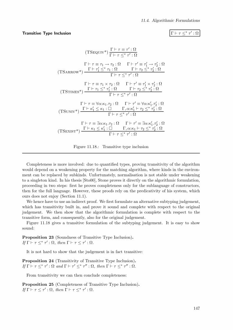
11.4. Algorithmic Formulations
Transitive Type Inclusion Γ ⊢ τ ≤∗ τ ′ : Ω
(TSequiv*)Γ ⊢ τ ≡ τ ′ : Ω
Γ ⊢ τ ≤∗ τ ′ : Ω
(TSarrow*)
Γ ⊢ τ ≡ τ1 → τ2 : Ω Γ ⊢ τ ′ ≡ τ ′1 → τ ′2 : ΩΓ ⊢ τ ′1 ≤∗ τ1 : Ω Γ ⊢ τ2 ≤∗ τ ′2 : Ω
Γ ⊢ τ ≤∗ τ ′ : Ω
(TStimes*)
Γ ⊢ τ ≡ τ1 × τ2 : Ω Γ ⊢ τ ′ ≡ τ ′1 × τ ′2 : ΩΓ ⊢ τ1 ≤∗ τ ′1 : Ω Γ ⊢ τ2 ≤∗ τ ′2 : Ω
Γ ⊢ τ ≤∗ τ ′ : Ω
(TSuniv*)
Γ ⊢ τ ≡ ∀α:κ1.τ2 : Ω Γ ⊢ τ ′ ≡ ∀α:κ′1.τ′2 : Ω
Γ ⊢ κ′1 ≤ κ1 : Γ, α:κ′1 ⊢ τ2 ≤∗ τ ′2 : Ω
Γ ⊢ τ ≤∗ τ ′ : Ω
(TSexist*)
Γ ⊢ τ ≡ ∃α:κ1.τ2 : Ω Γ ⊢ τ ′ ≡ ∃α:κ′1.τ′2 : Ω
Γ ⊢ κ1 ≤ κ′1 : Γ, α:κ1 ⊢ τ2 ≤∗ τ ′2 : Ω
Γ ⊢ τ ≤∗ τ ′ : Ω
Figure 11.18.: Transitive type inclusion
Completeness is more involved: due to quantified types, proving transitivity of the algorithmwould depend on a weakening property for the matching algorithm, where kinds in the environ-ment can be replaced by subkinds. Unfortunately, normalisation is not stable under weakeningto a singleton kind. In his thesis [Sto00], Stone proves it directly on the algorithmic formulation,proceeding in two steps: first he proves completeness only for the sublanguage of constructors,then for the full language. However, these proofs rely on the predicativity of his system, whichours does not enjoy (Section 11.1).
We hence have to use an indirect proof. We first formulate an alternative subtyping judgement,which has transitivity built in, and prove it sound and complete with respect to the originaljudgement. We then show that the algorithmic formulation is complete with respect to thetransitive form, and consequently, also for the original judgement.
Figure 11.18 gives a transitive formulation of the subtyping judgement. It is easy to showsound:
Proposition 23 (Soundness of Transitive Type Inclusion).If Γ ⊢ τ ≤∗ τ ′ : Ω, then Γ ⊢ τ ≤ τ ′ : Ω.
It is not hard to show that the judgement is in fact transitive:
Proposition 24 (Transitivity of Transitive Type Inclusion).If Γ ⊢ τ ≤∗ τ ′ : Ω and Γ ⊢ τ ′ ≤∗ τ ′′ : Ω, then Γ ⊢ τ ≤∗ τ ′′ : Ω.
From transitivity we can then conclude completeness:
Proposition 25 (Completeness of Transitive Type Inclusion).If Γ ⊢ τ ≤ τ ′ : Ω, then Γ ⊢ τ ≤∗ τ ′ : Ω.
147
11. The Type Language
Finally, we show completeness of the type matching algorithm by relating it to the transitivejudgement:
Theorem 26 (Completeness of Algorithmic Type Matching).
1. If Γ ⊢ τ ≤∗ τ ′ : Ω, then Γ ⊲ τ ≤ τ ′ Ω.
2. If Γ ⊢ τ ≤∗ τ ′ : Ω, then Γ ⊲ τ π and Γ ⊲ τ ′ π′ and Γ ⊲ π ⊑ π′.
3. If Γ ⊢ τ ≤ τ ′ : κ, then Γ ⊲ τ ≤ τ ′ κ.
From completeness of kind and type matching follows decidability:
Proposition 27 (Decidability of Type Inclusion).Given Γ ⊢ τ : κ and Γ ⊢ τ ′ : κ, it is decidable whether Γ ⊢ τ ≤ τ ′ : κ holds.
11.5. Related Work
11.5.1. Typed Lambda Calculi
There exists countless works on λ-calculi, type systems, and their use as models for programminglanguages. We refer the reader to two standard references, namely Barendregt’s handbookchapter on Lambda Calculi with Types [Bar92], which presents the basic theory from untypedcalculus to dependent types and the lambda cube, and Pierce’ book on Types and ProgrammingLanguages [Pie02], which gives an introduction to, and extensive overview of, the use of lambdacalculus as an idealised programming language, particularly exploring different dimensions oftype systems.
11.5.2. Singletons
Singleton types were first proposed as a means for expressing modular specifications by As-pinall [Asp95, Asp97]. He introduces higher-order singletons S(M : A) as primitive,3 whichproduces the minor technical complication that there is an infinite sequence of subtypesS(M : A) ≥ S(M : S(M : A)) ≥ . . . that has to be tamed by making all its elements equivalentwith an additional rule. Interestingly, his system does not have a separate equivalence judge-ment, but encodes it as validity of the form Γ ⊢ M : S(M ′ : A). The system does not haveη-equivalence.
As already mentioned, our system is closely based on the work of Stone & Harper [SH06].They introduce a simple lambda calculus with singleton types. The kind language of our systemis almost identical to their type language, except for the addition of abstraction kinds (andsingletons thereof). We adopted our type and kind equivalence algorithm directly from theirarticle, with only minor modifications to encompass the extensions. Our type language is richerthan their term language. However, with respect to equivalence and subkinding, the built-in typeconstructors of our type language can simply be treated as additional higher-order constantsthat do not affect the meta theory and algorithms. A variant of their system with a slightlyricher type language practically identical to ours (except for the lack of existential types) appearsin Stone’s chapter on Type Definitions [Sto05].
One substantial extension that our system adds to the picture is subtyping, which wouldcorrespond to a notion of “subterming”, or value subsumption, that does not exist in Stone& Harper’s system. However, in his thesis [Sto00] Stone studies a more complicated system
3He uses the syntax MA for this purpose.
148
11.6. Summary
featuring singleton kinds and singleton types, and subkinding as well as subtyping. He evendiscusses an extension with intensional type analysis. In a first approximation, our systemcan be seen as a subsystem of that one, except for the addition of abstraction kinds and typegenerativity. However, his system is predicative, while ours allows fully impredicative typeformation. That is crucial for our purposes, because we could not express dynamics (and hencepackages) with a predicative restriction – a package is represented by the polymorphic type∃α:Ω.α, and must be able to embed other polymorphic values. Thanks to predicativity, Stonecan prove completeness of the subtyping algorithm directly on the algorithmic formulation, whilewe were forced to take the detour through an auxiliary transitive subtyping judgement to showtransitivity of the algorithm.
Singletons have also been employed by Dreyer, Crary & Harper in their work on type sys-tems for higher-order modules [DCH03]. The language they describe consists of two layeredlanguages: terms and modules. Type equivalence depends on module equivalence, due to projec-tion of types from modules. Singletons appear in the module language, which induces dependentmodule types. Earlier work on higher-order module systems used translucent sums [HS00, Lil97]or, equivalently, manifest types [Ler94, Ler95] instead of singletons. They can basically be in-terpreted as a restricted form of singletons that can only be introduced in syntactically explicitpositions, and thus are somewhat more tractable.
11.5.3. Type Names, Environment and Abstraction Kinds
Many systems deal with type names for which an isomorphism must be recorded in the en-vironment. For example, Stone describes a simple system that deals with type definitions byrecording them as special entries in the environment [Sto05], but the types are just synonymsfor existing types.
In previous work [Ros03], we also used special environment entries of the form α ≈ τ to recordgenerated type names and their representations. Vytiniotis, Washburn & Weirich use a separatetype isomorphism environment for the same purpose [VWW05]. In both works, type names canonly be used for coercing between the type and its representation.
Dreyer also expresses type abstraction with explicit type generation to cope with recursivemodules [Dre07]. For that purpose, he separates generation from definition of abstract typenames, and hence requires multiple different environment entries that realise a simple effectsystem to ensure linearity of the bindings. See Section 12.10.3 for a more detailed comparison.
Where type names merely act as synonyms, singleton kinds represent a more uniform alterna-tive to specialised environment entries. We are not aware of any previous work that has appliedthe same generalisation to non-synonym type names, thus arriving at a notion equivalent to ourabstraction kinds.
11.6. Summary
• The type language of λωSAΨ is impredicative and higher-order with the usual built-in con-
structors, and including type pairs.
• The kind level has singleton kinds and abstraction kinds and is dependently kinded.
• Singletons induce subkinding and subtyping.
• Higher-order singletons are definable as a derived concept.
• Abstraction kinds classify explicit type isomorphisms.
149
11. The Type Language
• Standard βη-rules for type functions and pairs are derivable thanks to singletons.
• The judgements of the system are Environment, Kind and Type Validity, Type and KindEquivalence, Type and Kind Inclusion.
• We give algorithms for deciding all judgements of the type system.
150
12. The Term Language
In this chapter we present the term level of our calculus, its typing rules, and the operationalsemantics. Again, most of the system is fairly standard, and we concentrate the discussion onour additions: type analysis, type generation, coercions, and pickling.
We then state standard soundness properties for the operational semantics, which are essen-tially straightforward given the type system meta theory developed in the last chapter. However,we first have to know that the type system is decidable, since unpickling has to perform typechecking for verification.1 Hence, we develop an algorithmic formulation of the typing rules.
Finally, we give a moderate abstraction result that establishes that type generation and co-ercions are indeed sufficient to ensure abstraction safety. Similar to the last chapter, auxiliarypropositions and all proofs can be found in Appendix D.
12.1. Typing
Figure 12.1 shows the syntax of our term language. It consists of the standard constructions fromSystem Fω – functions, pairs, polymorphic abstractions, existential packages – enriched with typeanalysis, type generation, coercions, and pickles with respective operations. For symmetry withexistential types, pairs are eliminated by a pattern matching let construct instead of projection.We discuss the other extensions individually in the following sections.
Well-formedness and typing of terms is specified by the rules of the term validity judgement,Γ ⊢ e : τ (Figure 12.2). Besides the non-standard extensions, whose semantics we will describein the following sections, the rules bear little surprises. The only exception is rule Eclose
for forming existentials, which takes advantage of the presence of singleton kinds to assign aunique (principal) type without requiring the usual annotation. This corresponds closely to thesituation in ML, where a structure expression always is assigned a fully transparent signature.
In several places it will become convenient to have a unit type available. Also, a conventionallet-expression will come in handy. We assume the following encodings:
1 := ∀α:Ω. α→ α
⋄ := λα:Ω. λx:α. x
letx = e1 in e2 := let〈x, 〉 = 〈e1, ⋄〉 in e2
Similar to the other judgements of the system (Chapter 11), the structure of the typing rulesimplies that the classifying type τ derived by the judgement is valid under the environment Γ:
Proposition 28 (Validity of Term Validity Rules).If Γ ⊢ e : τ , then Γ ⊢ τ : Ω.
12.1.1. Principality
A technical problem with the rich type language in our calculus is that it does not automaticallylead to principal (or least) types. There are two problems.
1As noted in Chapter 3, the type system of Alice ML is in fact undecidable. For the calculus, we prefer a“cleaner” approach, especially since abstract signatures, which make Alice ML undecidable, are rather ofcursory utility.
151
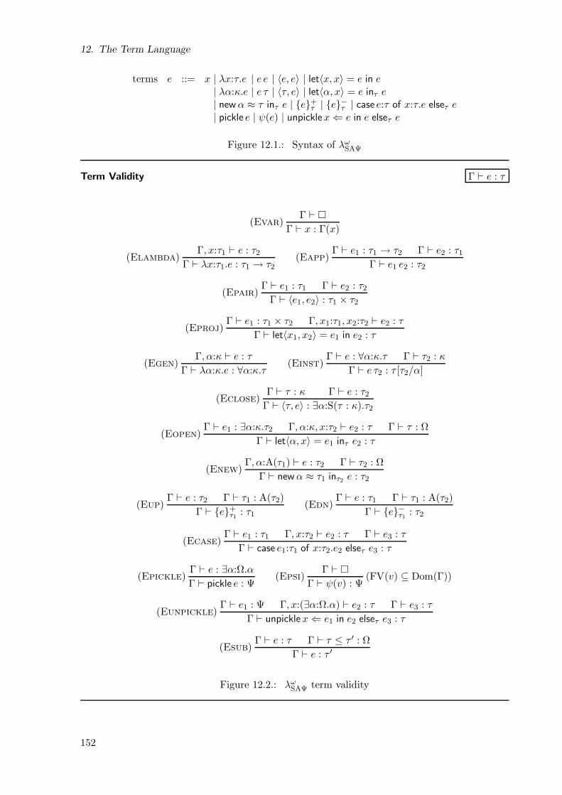
12. The Term Language
terms e ::= x | λx:τ.e | e e | 〈e, e〉 | let〈x, x〉 = e in e| λα:κ.e | e τ | 〈τ, e〉 | let〈α, x〉 = e inτ e| newα ≈ τ inτ e | e
+τ | e−τ | case e:τ of x:τ.e elseτ e
| pickle e | ψ(e) | unpicklex⇐ e in e elseτ e
Figure 12.1.: Syntax of λωSAΨ
Term Validity Γ ⊢ e : τ
(Evar)Γ ⊢
Γ ⊢ x : Γ(x)
(Elambda)Γ, x:τ1 ⊢ e : τ2
Γ ⊢ λx:τ1.e : τ1 → τ2(Eapp)
Γ ⊢ e1 : τ1 → τ2 Γ ⊢ e2 : τ1Γ ⊢ e1 e2 : τ2
(Epair)Γ ⊢ e1 : τ1 Γ ⊢ e2 : τ2
Γ ⊢ 〈e1, e2〉 : τ1 × τ2
(Eproj)Γ ⊢ e1 : τ1 × τ2 Γ, x1:τ1, x2:τ2 ⊢ e2 : τ
Γ ⊢ let〈x1, x2〉 = e1 in e2 : τ
(Egen)Γ, α:κ ⊢ e : τ
Γ ⊢ λα:κ.e : ∀α:κ.τ(Einst)
Γ ⊢ e : ∀α:κ.τ Γ ⊢ τ2 : κ
Γ ⊢ e τ2 : τ [τ2/α]
(Eclose)Γ ⊢ τ : κ Γ ⊢ e : τ2
Γ ⊢ 〈τ, e〉 : ∃α:S(τ : κ).τ2
(Eopen)Γ ⊢ e1 : ∃α:κ.τ2 Γ, α:κ, x:τ2 ⊢ e2 : τ Γ ⊢ τ : Ω
Γ ⊢ let〈α, x〉 = e1 inτ e2 : τ
(Enew)Γ, α:A(τ1) ⊢ e : τ2 Γ ⊢ τ2 : Ω
Γ ⊢ newα ≈ τ1 inτ2 e : τ2
(Eup)Γ ⊢ e : τ2 Γ ⊢ τ1 : A(τ2)
Γ ⊢ e+τ1 : τ1
(Edn)Γ ⊢ e : τ1 Γ ⊢ τ1 : A(τ2)
Γ ⊢ e−τ1 : τ2
(Ecase)Γ ⊢ e1 : τ1 Γ, x:τ2 ⊢ e2 : τ Γ ⊢ e3 : τ
Γ ⊢ case e1:τ1 of x:τ2.e2 elseτ e3 : τ
(Epickle)Γ ⊢ e : ∃α:Ω.α
Γ ⊢ pickle e : Ψ(Epsi)
Γ ⊢
Γ ⊢ ψ(v) : Ψ(FV(v) ⊆ Dom(Γ))
(Eunpickle)Γ ⊢ e1 : Ψ Γ, x:(∃α:Ω.α) ⊢ e2 : τ Γ ⊢ e3 : τ
Γ ⊢ unpicklex⇐ e1 in e2 elseτ e3 : τ
(Esub)Γ ⊢ e : τ Γ ⊢ τ ≤ τ ′ : Ω
Γ ⊢ e : τ ′
Figure 12.2.: λωSAΨ term validity
152
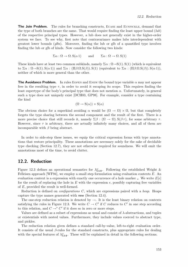
12.2. Reduction
The Join Problem. The rules for branching constructs, Ecase and Eunpickle, demand thatthe type of both branches are the same. That would require finding the least upper bound (lub)of the respective principal types. However, a lub does not generally exist in the higher-ordersystem we face. To see why, first note that contravariance makes lubs interdependent withgreatest lower bounds (glbs). Moreover, finding the lub or glb of a quantified type involvesfinding the lub or glb of kinds. Now consider the following two kinds:
Σα : Ω → Ω.S(α 1) and Σα : Ω → Ω.S(1)
These kinds have at least two common subkinds, namely Σα : Ω→S(1).S(1) (which is equivalentto Σα : Ω→S(1).S(α 1)) and Σα : (Πβ:Ω.S(β)).S(1) (equivalent to Σα : (Πβ:Ω.S(β)).S(α 1)),neither of which is more general than the other.
The Avoidance Problem. In rules Eopen and Enew the bound type variable α may not appearfree in the resulting type τ , in order to avoid it escaping its scope. This requires finding theleast supertype of the body’s principal type that does not mention α. Unfortunately, in generalsuch a type does not uniquely exist [DCH03, GP98]. For example, consider a type containingthe kind
(Ω → S(α)) × S(α)
The obvious choice for a superkind avoiding α would be (Ω → Ω) × Ω, but that completelyforgets the type sharing between the second component and the result of the first. There is amore precise choice that still records it, namely Σβ : (Ω → Ω).S(β τ), for some arbitrary τ .However, since τ is arbitrary, there are actually infinitely many choices, and all of them areincomparable with β being abstract.
In order to side-step these issues, we equip the critical expression forms with type annota-tions that restore principality. These annotations are necessary solely for the sake of decidabletype checking (Section 12.7), they are not otherwise required for soundness. We will omit theannotations most of the time, to avoid clutter.
12.2. Reduction
Figure 12.3 defines an operational semantics for λωSAΨ. Following the established Wright &
Felleisen approach [WF94], we employ a small step formulation using evaluation contexts E. Anevaluation context is a expression with exactly one occurrence of a hole marker . We write E[e]for the result of replacing the hole in E with the expression e, possibly capturing free variablesof E, provided the result is well-formed.
Reduction is defined on configurations C, which are expressions paired with a heap. Heapscapture the type names generated with new (Section 12.4).
The one-step reduction relation is denoted by →. It is the least binary relation on contextssatisfying the rules in Figure 12.3. We write C → C ′ if C reduces to C ′ in one step accordingto this relation, and C →∗ C ′ if it does so in zero or more steps.
Values are defined as a subset of expressions as usual and consist of λ-abstractions, and tuplesor existentials with nested values. Furthermore, they include values coerced to abstract type,and pickles.
The reduction relation given defines a standard call-by-value, left-to-right evaluation order.It consists of the usual β-rules for the standard constructs, plus appropriate rules for dealingwith the special features of λω
SAΨ. These will be explained in detail in the following sections.
153
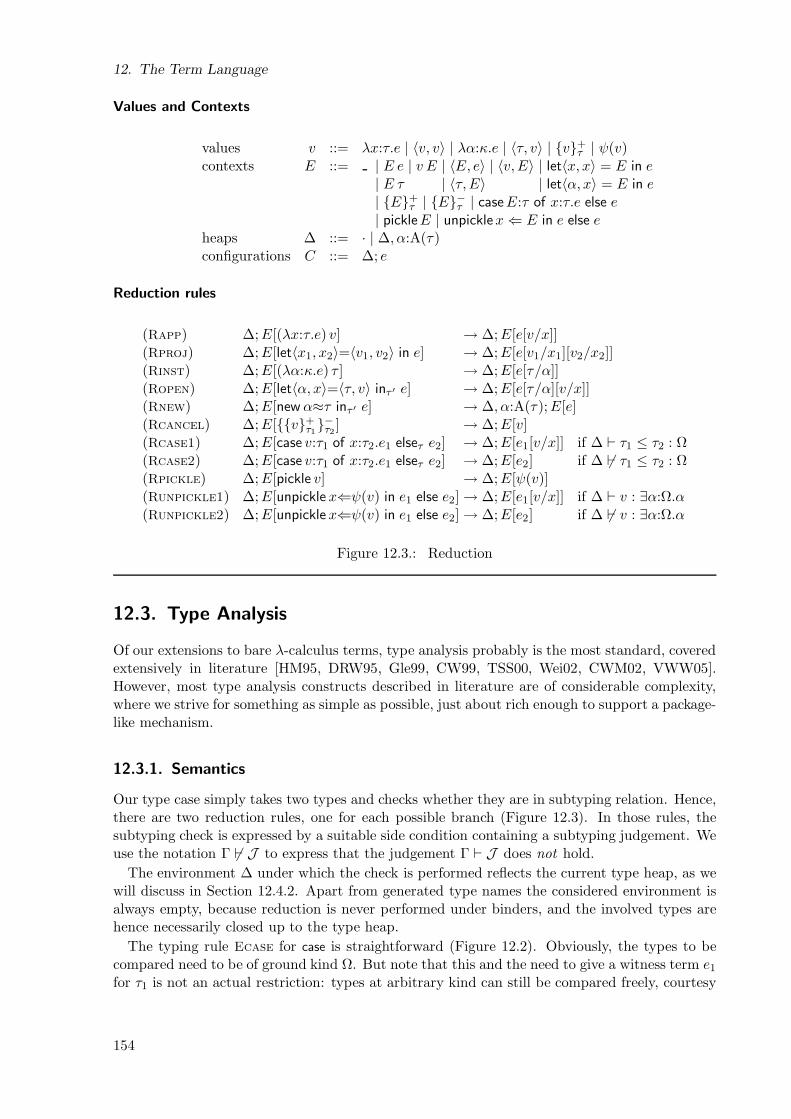
12. The Term Language
Values and Contexts
values v ::= λx:τ.e | 〈v, v〉 | λα:κ.e | 〈τ, v〉 | v+τ | ψ(v)
contexts E ::= | E e | v E | 〈E, e〉 | 〈v,E〉 | let〈x, x〉 = E in e| E τ | 〈τ,E〉 | let〈α, x〉 = E in e| E+
τ | E−τ | caseE:τ of x:τ.e else e| pickleE | unpicklex⇐ E in e else e
heaps ∆ ::= · | ∆, α:A(τ)configurations C ::= ∆; e
Reduction rules
(Rapp) ∆;E[(λx:τ.e) v] → ∆;E[e[v/x]](Rproj) ∆;E[let〈x1, x2〉=〈v1, v2〉 in e] → ∆;E[e[v1/x1][v2/x2]](Rinst) ∆;E[(λα:κ.e) τ ] → ∆;E[e[τ/α]](Ropen) ∆;E[let〈α, x〉=〈τ, v〉 inτ ′ e] → ∆;E[e[τ/α][v/x]](Rnew) ∆;E[new α≈τ inτ ′ e] → ∆, α:A(τ);E[e](Rcancel) ∆;E[v+
τ1−τ2 ] → ∆;E[v]
(Rcase1) ∆;E[case v:τ1 of x:τ2.e1 elseτ e2] → ∆;E[e1[v/x]] if ∆ ⊢ τ1 ≤ τ2 : Ω(Rcase2) ∆;E[case v:τ1 of x:τ2.e1 elseτ e2] → ∆;E[e2] if ∆ 6⊢ τ1 ≤ τ2 : Ω(Rpickle) ∆;E[pickle v] → ∆;E[ψ(v)](Runpickle1) ∆;E[unpickle x⇐ψ(v) in e1 else e2] → ∆;E[e1[v/x]] if ∆ ⊢ v : ∃α:Ω.α(Runpickle2) ∆;E[unpickle x⇐ψ(v) in e1 else e2] → ∆;E[e2] if ∆ 6⊢ v : ∃α:Ω.α
Figure 12.3.: Reduction
12.3. Type Analysis
Of our extensions to bare λ-calculus terms, type analysis probably is the most standard, coveredextensively in literature [HM95, DRW95, Gle99, CW99, TSS00, Wei02, CWM02, VWW05].However, most type analysis constructs described in literature are of considerable complexity,where we strive for something as simple as possible, just about rich enough to support a package-like mechanism.
12.3.1. Semantics
Our type case simply takes two types and checks whether they are in subtyping relation. Hence,there are two reduction rules, one for each possible branch (Figure 12.3). In those rules, thesubtyping check is expressed by a suitable side condition containing a subtyping judgement. Weuse the notation Γ 6⊢ J to express that the judgement Γ ⊢ J does not hold.
The environment ∆ under which the check is performed reflects the current type heap, as wewill discuss in Section 12.4.2. Apart from generated type names the considered environment isalways empty, because reduction is never performed under binders, and the involved types arehence necessarily closed up to the type heap.
The typing rule Ecase for case is straightforward (Figure 12.2). Obviously, the types to becompared need to be of ground kind Ω. But note that this and the need to give a witness term e1for τ1 is not an actual restriction: types at arbitrary kind can still be compared freely, courtesy
154
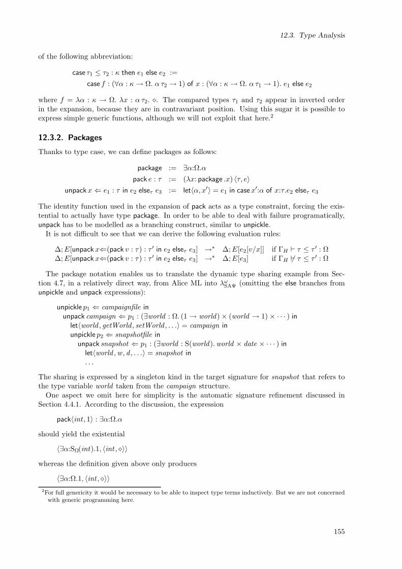
12.3. Type Analysis
of the following abbreviation:
case τ1 ≤ τ2 : κ then e1 else e2 :=
case f : (∀α : κ→ Ω. α τ2 → 1) of x : (∀α : κ→ Ω. α τ1 → 1). e1 else e2
where f = λα : κ → Ω. λx : α τ2. ⋄. The compared types τ1 and τ2 appear in inverted orderin the expansion, because they are in contravariant position. Using this sugar it is possible toexpress simple generic functions, although we will not exploit that here.2
12.3.2. Packages
Thanks to type case, we can define packages as follows:
package := ∃α:Ω.α
pack e : τ := (λx: package .x) 〈τ, e〉
unpackx⇐ e1 : τ in e2 elseτ e3 := let〈α, x′〉 = e1 in case x′:α of x:τ.e2 elseτ e3
The identity function used in the expansion of pack acts as a type constraint, forcing the exis-tential to actually have type package. In order to be able to deal with failure programatically,unpack has to be modelled as a branching construct, similar to unpickle.
It is not difficult to see that we can derive the following evaluation rules:
∆;E[unpackx⇐(pack v : τ) : τ ′ in e2 elseτ e3] →∗ ∆;E[e2[v/x]] if ΓH ⊢ τ ≤ τ ′ : Ω∆;E[unpackx⇐(pack v : τ) : τ ′ in e2 elseτ e3] →∗ ∆;E[e3] if ΓH 6⊢ τ ≤ τ ′ : Ω
The package notation enables us to translate the dynamic type sharing example from Sec-tion 4.7, in a relatively direct way, from Alice ML into λω
SAΨ (omitting the else branches fromunpickle and unpack expressions):
unpickle p1 ⇐ campaignfile inunpack campaign ⇐ p1 : (∃world : Ω. (1 → world) × (world → 1) × · · · ) in
let〈world , getWorld , setWorld , . . .〉 = campaign inunpickle p2 ⇐ snapshotfile in
unpack snapshot ⇐ p1 : (∃world : S(world).world × date × · · · ) inlet〈world ,w , d , . . .〉 = snapshot in. . .
The sharing is expressed by a singleton kind in the target signature for snapshot that refers tothe type variable world taken from the campaign structure.
One aspect we omit here for simplicity is the automatic signature refinement discussed inSection 4.4.1. According to the discussion, the expression
pack〈int , 1〉 : ∃α:Ω.α
should yield the existential
〈∃α:SΩ(int).1, 〈int , ⋄〉〉
whereas the definition given above only produces
〈∃α:Ω.1, 〈int , ⋄〉〉
2For full genericity it would be necessary to be able to inspect type terms inductively. But we are not concernedwith generic programming here.
155
12. The Term Language
Implementing such refinement generically would require to extract and separate the kind in-formation Stat(τ) embedded in an arbitrary type τ – which basically means defining a propermodule language by an appropriate inductive phase splitting translation. We give a sketch ofsuch a definition in Appendix B. Short of that, a properly refined package type can always begiven directly.
12.3.3. Recursion
Our type case operator is a variant of Girard’s J operator [Gir71, HM99] (Section 12.10.1).Girard showed that a profound implication of the J operator (and the corresponding loss ofparametericity, Section 10.5) is that – unlike plain Fω– a calculus providing it is no longerterminating. In particular, it is easy to construct a fixed point operator, say on type int →int [ACPP89]. In our system the following is one possible definition (for better readability, weuse the package notation defined in the previous section):
fixint→int = λf : (int→int) → (int→int).let f ′ =λp : package . λx : int .
unpack f ′ ⇐ p : package → (int→int) in f (f ′ p)x else 0in f ′ (pack f ′ : package → (int→int))
It is easy to check that this term is well-typed, and that its application to a suitable functionmeets the standard fixed point equation. The basic trick of the encoding is that the recursivetype usually needed to construct fix is avoided by hiding the recursive occurrence inside thepackage type – thanks to type case, we can still recover it dynamically.
Analogously, we can define a fixed point operator fixτ1→τ2 for any types τ1, τ2 where τ2 is in-habited. We will write ⊥τ for a diverging computation of type τ , which can easily be constructedfrom fix1→τ as follows:
⊥τ = fix1→τ (λf : 1 → τ. λx : 1. f x) ⋄
With this encoding, recursion and divergence are restricted to inhabited types, for whicha witness value is available (as a default value for the else branch of the unpack inside fix,although it will never be reached). It is easy to see that a general fixed point operator cannot beexpressed, because the type case does not allow the construction of terms that would otherwisebe uninhabited – the constituent term e3 needs to be a witness of the whole expression’s resulttype [HM99]. For our purposes, this limited form of recursion is good enough. It would bestraightforward to add a primitive fixed point operator to the calculus if needed.
12.4. Type Generation
The next feature we turn to is type generation. It is supported in our calculus through a singlesyntactic construct, namely new expressions.
12.4.1. Type Heap
Evaluating new is supposed to generate a fresh type. We employ an additional heap in whichgenerated types are allocated. The heap is simply a list of type variables classified by abstractionkinds. A configuration ∆; e then represents a snapshot of a computation. We consider the heap∆ in a configuration as a (multiple) binder, and hence configurations are equivalent moduloα-renaming.
156

12.4. Type Generation
Typing can be extended to configurations by the following straightforward rule, which takesadvantage of the fact that heaps are a syntactic subclass of environments:
(Cvalid)Γ,∆ ⊢ e : τ
Γ ⊢ ∆; e : τ
Thanks to Environment Validity (Section 11.1.1), the premise enforces that ∆ is well-formed.As an example of a computation involving the heap, consider the following reduction sequence:
·; (λf :int→int .f (newα ≈ int in f 4)) (λx:int . new β ≈ bool in x)→ (Rapp) ·; (λx:int . new β ≈ bool in x) (new α ≈ int in (λx:int . new β′ ≈ bool in x) 4)→ (Rnew) α:A(int); (λx:int . new β ≈ bool in x) ((λx:int . new β′ ≈ bool in x) 4)→ (Rapp) α:A(int); (λx:int . new β ≈ bool in x) (new β′ ≈ bool in 4)→ (Rnew) α:A(int), β′:A(bool ); (λx:int . new β ≈ bool in x) 4→ (Rapp) α:A(int), β′:A(bool ), β:A(bool ); 4
It terminates with a configuration of the form ∆; v, where v = 4 is the resulting value, and∆ = α:A(int), β′:A(bool ), β:A(bool ) represents the created type heap containing the three newtypes named α, β and β′. Note that, thanks to the variable convention and appropriate α-conversion, the generated types are all different, although β and β′ both stem from the sameexpression and have the same representation bool .
It should be noted that type generation is fully dynamic, i.e. the number of type names gen-erated is neither determined statically nor bounded. The following non-terminating expressionwill actually generate an infinite number of types:
(fix1→1 λf :1→1.λx:1. new α ≈ τ in f x) ⋄
12.4.2. Analysing Generated Types
The whole point about introducing dynamically generated types is to make them available inthe subtyping check performed by type case. Thus we must allow the types in a case expressionto refer to names from the heap. Consequently, the reduction rules for type case must embracethe heap. More precisely, the side conditions expressing the subtyping check must be using asuitable heap environment reflecting the bindings in the heap. Fortunately, since heaps havebeen defined such that they form a syntactic subclass of environments, we can use a heap ∆ asan environment directly in the rules.
Let us return to our previous example, which resulted in
∆; v = α:A(int), β′:A(bool ), β:A(bool ); 4
Obviously, a dynamic type test comparing the generated types, for instance,
∆; caseβ ≤ β′ : Ω then 1 else 0
(using the abbreviation defined in Section 12.3.1) will evaluate to 0 as desired, because ∆ ⊢ β ≤β′ : cannot be derived – the two types are incompatible. Note how this behaviour correspondsto the static semantics of generative functors in ML, where
functor F () = struct type t = bool end :> sig type t end
structure M1 = F ()structure M2 = F ()
yields incompatible types M1.t and M2.t.In Section 12.9 we will state formally that generated types maintain abstraction safety.
157

12. The Term Language
12.5. Coercions
To construct values of abstract type, values of the corresponding representation type have to becoerced into the new type. Our calculus demands such coercions to be explicit. An extensivediscussion of this design choice is only possible when considering higher-order abstraction, andhence appears in Section 13.6.1.
There are two symmetric expression forms, with dual typing rules:
(Eup)Γ ⊢ e : τ ′ Γ ⊢ τ : A(τ ′)
Γ ⊢ e+τ : τ
(Edn)Γ ⊢ e : τ Γ ⊢ τ : A(τ ′)
Γ ⊢ e−τ : τ ′
Upward and downward coercions can be seen as the introduction and elimination forms ofabstract types. An upward coercion v+
τ , where v is a value, is considered a value. Such avalue can be eliminated by the respective downward coercion, thanks to the Rcancel reductionrule.
Due to the side conditions in the rules, coercions are only available within the lexical scopeof the corresponding type generator, thus the transition across abstraction boundaries can onlybe triggered within the lexical scope of the generator, which is the crucial property ensuringabstraction. Moreover, the type system guarantees that only coercions belonging to the sametype can cancel each other out.
Note that the type τ used for coercion is not necessarily a type variable, although ultimatelyonly new can create types of abstraction kind, which have to be referred to as variables. However,due to the higher-order nature of our type system, τ may still be an arbitrary type expression,as in
λα : Ω → A(int). λx : α bool . 13+α bool
12.6. Pickling
The last feature of our calculus is pickling. Pickles are values of type Ψ, as the correspondingtyping rules reveal (Figure 12.2). The content of a pickle, however, always has to be an expressionof type ∃α:Ω.α – that is, a package.
The rule Epsi does not require the embedded value v to be well-formed, hence modellingpotentially malformed pickles. To simplify manners however, the rule syntactically restrictspickle values to be closed with respect to the environment Γ. This is to maintain the usualVariable Containment property, which states that all free variables of a well-formed term arebound by the environment (Appendix C.1).
Reduction rules for pickling implement the expected semantics (Figure 12.3): pickle justreduces to a pickle value (rule Rpickle), and unpickle branches dependent on whether the picklecontains a well-formed package (rules Runpickle1 and Runpickle2). Similar to the subtypingcheck performed by type case (Section 12.3), this is expressed by a side condition consisting ofa suitable typing judgement for the pickled value. And like for type case, the side condition hasto embrace the type heap, because pickles may refer to abstract types (in the value as well asthe type of the embedded package).
To clarify the interplay between dynamic type checking and dynamic type matching whenaccessing a pickled package, consider the following four examples (for brevity we omit branchesand variable binding of the unpack and unpickle operations):
1. unpack (unpickle pickle(packλx:1.⋄ : 1→1)) : 1→1
2. unpack (unpickle pickle(packλx:1.⋄ : 1→1)) : 1→1→1
3. unpack (unpickle ψ(packλx:1.x ⋄ : 1→1)) : 1→1
158
12.7. Algorithmic Type Checking
4. unpack (unpickle pickle(packλx:1.x ⋄ : 1→1)) : 1→1
The first three expressions are all (statically) well-typed, but only the first will evaluate success-fully. The second will fail due to a dynamic type error in unpack, the third due to a verificationerror during unpickling. The last example is rejected by the (static) type system, because thepickled value is not denoted by a well-formed expression. Contrast this to the third example,which represents a (statically valid) malformed pickle.
12.7. Algorithmic Type Checking
One of the most unusual aspects of pickling is that the operational semantics of λωSAΨ may involve
type-checking arbitrary expressions. We saw that this is simply expressed as a side condition inthe reduction rules Runpickle1 and Runpickle2 (Figure 12.3). To make the rules well-definedhowever (and thus for soundness), we have to show that this side condition is in fact decidable.That is, we have to give an algorithm for type checking λω
SAΨ-terms.
Figure 12.4 shows the type checking algorithm. It consists of three judgements: the syntax-directed type synthesis judgement Γ ⊲ e τ computes a (principal) type τ for a given term e.The auxiliary type analysis judgement Γ ⊲ e τ checks a term against a required type τ , up tosubtyping. Finally, another auxiliary judgement derives a principal type in weak-head normalform. It is used where a premise requires a type of a particular shape. The main structuraldifference to the declarative formulation is the usual removal of the subsumption rule, which hasbeen built-in into the rules where it is actually needed.
Correctness of the algorithm is relatively straightforward to show.
Theorem 29 (Soundness of Algorithmic Type Synthesis).Let Γ ⊢ .
1. If Γ ⊲ e τ , then Γ ⊢ e : τ .
2. If Γ ⊲ e π, then Γ ⊢ e : π.
3. If Γ ⊲ e τ with Γ ⊢ τ : Ω, then Γ ⊢ e : τ .
Theorem 30 (Completeness of Algorithmic Type Synthesis).
1. If Γ ⊢ e : τ , then Γ ⊲ e τ ′ with Γ ⊢ τ ′ ≤ τ : Ω.
2. If Γ ⊢ e : τ , then Γ ⊲ e π with Γ ⊢ π ≤ τ : Ω.
3. If Γ ⊢ e : τ and Γ ⊢ τ ≤ τ ′ : Ω, then Γ ⊲ e τ ′.
Because the algorithm is syntax-directed, it terminates, and hence implies decidability:
Corollary 31 (Decidability of Term Validity).
1. Given e and Γ ⊢ , it is decidable whether there is a τ such that Γ ⊢ e : τ holds.
2. Given e and Γ ⊢ and Γ ⊢ τ : Ω, it is decidable whether Γ ⊢ e : τ holds.
159
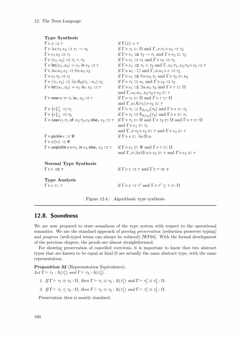
12. The Term Language
Type Synthesis
Γ ⊲ x τ if Γ(x) = τΓ ⊲ λx:τ1.e2 τ1 → τ2 if Γ ⊲ τ1 Ω and Γ, x:τ1 ⊲ e2 τ2Γ ⊲ e1 e2 τ1 if Γ ⊲ e1 τ2 → τ1 and Γ ⊲ e2 τ2Γ ⊲ 〈e1, e2〉 τ1 × τ2 if Γ ⊲ e1 τ1 and Γ ⊲ e2 τ2Γ ⊲ let〈x1, x2〉 = e1 in e2 τ if Γ ⊲ e1 τ1 × τ2 and Γ, x1:τ1, x2:τ2 ⊲ e2 τΓ ⊲ λα:κ1.e2 ∀α:κ1.τ2 if Γ ⊲ κ1 : and Γ, α:κ1 ⊲ e τ2Γ ⊲ e1 τ2 τ1 if Γ ⊲ e1 ∀α:κ2.τ1 and Γ ⊲ τ2 κ2
Γ ⊲ 〈τ1, e2〉 ∃α:SΩ(τ1 : κ1).τ2 if Γ ⊲ τ1 κ1 and Γ ⊲ e2 τ2Γ ⊲ let〈α1, x2〉 = e1 inτ e2 τ if Γ ⊲ e1 ∃α:κ1.τ2 and Γ ⊲ τ Ω
and Γ, α1:κ1, x2:τ2 ⊲ e2 τΓ ⊲ newα ≈ τ1 inτ e2 τ if Γ ⊲ τ1 Ω and Γ ⊲ τ Ω
and Γ, α:A(τ1) ⊲ e2 τΓ ⊲ e+
τ1 τ1 if Γ ⊲ τ1 SA(τ2)(τ3) and Γ ⊲ e τ2Γ ⊲ e−τ1 τ2 if Γ ⊲ τ1 SA(τ2)(τ3) and Γ ⊲ e τ1Γ ⊲ case e1:τ1 of x2:τ2.e2 elseτ e3 τ if Γ ⊲ τ1 Ω and Γ ⊲ τ2 Ω and Γ ⊲ τ Ω
and Γ ⊲ e1 τ1and Γ, x:τ2 ⊲ e2 τ and Γ ⊲ e3 τ
Γ ⊲ pickle e Ψ if Γ ⊲ e ∃α:Ω.αΓ ⊲ ψ(v) ΨΓ ⊲ unpicklex⇐e1 in e2 elseτ e3 τ if Γ ⊲ e1 Ψ and Γ ⊲ τ Ω
and Γ, x:∃α:Ω.α ⊲ e2 τ and Γ ⊲ e3 τ
Normal Type Synthesis
Γ ⊲ e π if Γ ⊲ e τ and Γ ⊲ τ π
Type Analysis
Γ ⊲ e τ if Γ ⊲ e τ ′ and Γ ⊲ τ ′ ≤ τ Ω
Figure 12.4.: Algorithmic type synthesis
12.8. Soundness
We are now prepared to state soundness of the type system with respect to the operationalsemantics. We use the standard approach of proving preservation (reduction preserves typing)and progress (well-typed terms can always be reduced) [WF94]. With the formal developmentof the previous chapter, the proofs are almost straightforward.
For showing preservation of cancelled coercions, it is important to know that two abstracttypes that are known to be equal at kind Ω are actually the same abstract type, with the samerepresentation:
Proposition 32 (Representation Equivalence).Let Γ ⊢ τ1 : A(τ ′1) and Γ ⊢ τ2 : A(τ ′2).
1. If Γ ⊢ τ1 ≡ τ2 : Ω, then Γ ⊢ τ1 ≡ τ2 : A(τ ′1) and Γ ⊢ τ ′1 ≡ τ ′2 : Ω.
2. If Γ ⊢ τ1 ≤ τ2 : Ω, then Γ ⊢ τ1 ≡ τ2 : A(τ ′1) and Γ ⊢ τ ′1 ≡ τ ′2 : Ω.
Preservation then is mostly standard:
160
12.9. Opacity
Theorem 33 (Preservation).
1. If ∆ ⊢ e : τ and ∆; e→ ∆′; e′ with E = , then ∆′ ⊢ e′ : τ .
2. If · ⊢ C : τ and C → C ′, then · ⊢ C ′ : τ .
The progress proof requires the usual “canonical forms” lemma, but here respecting the heap:
Proposition 34 (Canonical Values).Let Γ ⊢ v : τ .
1. If Γ ⊢ τ ≤ τ ′ : Ω and Γ ⊢ τ ′ : A(τ1), then v = v1+τ2 .
2. If Γ ⊢ τ ≤ Ψ : Ω, then v = ψ(v1).
3. If Γ ⊢ τ ≤ τ1 → τ2 : Ω, then v = λx:τ ′1.e2.
4. If Γ ⊢ τ ≤ τ1 × τ2 : Ω, then v = 〈v1, v2〉.
5. If Γ ⊢ τ ≤ ∀α:κ1.τ2 : Ω, then v = λα:κ′1.e2.
6. If Γ ⊢ τ ≤ ∃α:κ1.τ2 : Ω, then v = 〈τ1, v2〉.
The formulation of the progress theorem also has to embrace the type heap:
Theorem 35 (Progress).If ∆ ⊢ e : τ , then either e = v, or (∆; e) = (∆;E[e1]) → (∆′;E[e′1]) = (∆′; e′).
The proof is mostly standard.
12.9. Opacity
By having proved soundness, we have shown that our calculus actually models a type safelanguage. But we have not yet shown that it also is abstraction safe (Section 1.1.1). We doso by formalising suitable notions of secrecy and authentication and proving them for values ofabstract type.
More precisely, we show a simple parametricity property that we call opacity. We consider aterm e that has free occurrences of a type variable α : Ω and a term variable x : α. The terme can be viewed as a client of some abstraction. If we now substitute the free variables by aconcrete implementation, then reduction of e will proceed disregardless of what implementationwe chose – as long as the type τ we substitute for α has abstraction kind (note that α is notassigned abstraction kind, otherwise e would logically be part of the implementation of theabstraction, and of course not opaque). Consequently, the client cannot have been able to lookat the representation type of α or access the value behind x.
However, this only gives secrecy. For authentication, we need to show that e can even usea function from the abstraction that expects a value of type α, without changing the outcomeof the evaluation either. We model this by allowing e to refer to a second variable f : α → 1.A function of this type can have two possible outcomes: termination (with ⋄) or divergence.By assuming that the substituted function terminates on the value substituted for x, but notmaking any assumptions for other possible values, we can prove authentication by observingthat reduction still proceeds uniformly – because if f was applied to a value different from xreduction would be unpredictable. Hence e can not have forged a value of type α.
161
12. The Term Language
Opacity, as stated below, combines these characterisations of secrecy and authentication intoa single formulation. It is a rather technical formulation, but the proof is essentially a straight-forward induction on derivations. Interestingly, the proof is completely independent from theuse of coercions. This indicates that (explicit) coercions are inessential to the system.
The core of the authentication half of the proof actually is a straightforward lemma showingthat we cannot construct a value of variable type α if α : Ω (note that the kind assumption iscrucial, as for a type of kind Sκ(τ) or A(τ) we often could write down a value).
Proposition 36 (Abstractness). If Γ = Γ1, α:Ω, x:α,Γ2 and Γ ⊢ e : τ with Γ ⊢ τ ≤ α, then e isnot a value.
For opacity itself, we only consider two different substitutions (i.e. implementations), since theresult obviously generalises to an arbitrary number of different substitutions. Because of typecase and unpickling, we must first show that type inclusion and term validity stay independentof the substitution as well.
Theorem 37 (Opacity).Let Γ = α:Ω, x:α, f :α→1, and γi = [αi/α] ∪ [vi/x] ∪ [v′i/f ] ∪ [α′ | α′ ∈ Dom(∆′)/α′] with∆, γi(∆
′) ⊢ γi : Γ,∆′ and ∆; v′i vi →∗ ∆; ⋄ for i ∈ 1, 2.
1. Let Γ,∆′ ⊢ τ : κ.If and only if ∆, γ1(∆
′) ⊢ γ1(τ) : γ1(κ), then ∆, γ2(∆′) ⊢ γ2(τ) : γ2(κ).
2. Let Γ,∆′ ⊢ τ : Ω and Γ,∆′ ⊢ τ ′ : Ω.If and only if ∆, γ1(∆
′) ⊢ γ1(τ) ≤ γ1(τ′) : Ω, then ∆, γ2(∆
′) ⊢ γ2(τ) ≤ γ2(τ′) : Ω.
3. Let Γ,∆′ ⊢ e : τ .If and only if ∆, γ1(∆
′) ⊢ γ1(e) : γ1(τ), then ∆, γ2(∆′) ⊢ γ2(e) : γ2(τ).
4. Let Γ,∆′ ⊢ e : τ .If and only if ∆, γ1(∆
′); γ1(e) →∗ ∆, γ1(∆
′),∆1; v′, then ∆1 = γ1(∆
′′) and v′ = γ1(v) with∆, γ2(∆
′); γ2(e) →∗ ∆, γ2(∆
′), γ2(∆′′); γ2(v).
Note that the opacity theorem assumes that the client – the expression e – has no accessto the type heap containing the abstract type substituted. This is an optimistic assumption.As we explained in Section 5.4, in practice an open scenario may, under certain circumstances,enable a malicious client to access parts of the type heap “out of scope”, and thus circumventopacity. The λω
SAΨ-calculus cannot directly express such a situation, though. We leave thedevelopment of an adequate refinement that may address this particular problem to future work(Section 14.2).
12.10. Related Work
12.10.1. Type Analysis and Dynamics
The type case construct in our calculus is a (weaker) variant of Girard’s J operator [Gir71,HM99]. Girard defines it as a constant of type ∀α:Ω.∀β:Ω.α → β with the following reductionrule:
J τ1 τ2 v → v if τ1 ≡ τ2J τ1 τ2 v → 0 τ2 if τ1 6≡ τ2
Here, 0 is an auxiliary universal constant of type ∀α:Ω.α, used as a default value instead of afailure branch.
162

12.10. Related Work
Even closer to our construct is a variant of J discussed by Mitchell & Harper [HM99]. Theiroperator TypeCond : ∀α:Ω.∀β:Ω.α→ β → β has the following reduction rules:
TypeCond τ1 τ2 v1 v2 → v1 if τ1 ≡ τ2TypeCond τ1 τ2 v1 v2 → v2 if τ1 6≡ τ2
This operator does not require a 0 constant, and modulo syntax is almost identical to ourtype case, except that we extend it with subtyping (and have higher-order types). Mitchell &Harper demonstrate that even the weaker TypeCond is sufficient to destroy normalization. Theypoint out that a type Dynamic implicitly introduces a form of impredicativity (since it can beexpressed as ∃α.α), and that impredicativity is essential for expressing diverging computations.
Richer forms of type analysis have been extensively discussed in programming language liter-ature, either as stand-alone constructs, or in conjunction with dynamics.
Dynamics were first formalised by Abadi, Cardelli Pierce & Plotkin [ACPP91]. In their system,dynamics were eliminated directly by a type case construct that allowed pattern matching onthe dynamic type. In the original system, only monomorphic types were possible, but they couldcontain pattern variables that captured constituent types. Later work by the same and otherauthors [ACPR95, LM93] extended this idea to polymorphic types, which raises a number ofissues about scoping of type and pattern variables. Abadi et al. also discuss the interaction withsubtyping, pointing out that subtyping interferes badly with pattern variables, because thereno longer always is a unique type to bind them to. Our type case supports subtyping, but nopattern variables, so no such problems arise.
Other works investigate type-based dispatch as a stand-alone feature. In particular, Harper &Morrisett introduce intensional type analysis as a more general construct for analysing types ortype variables [HM95]. Their main motivation is a typed intermediate language that can copewith heterogeneous representations in a compiler. Their system has a typerec construct that isnot simply a pattern matching construct, but a primitive recursion operator on higher-ordertypes. Moreover, they also introduce an analogous Typerec on the type level and show that manyinteresting applications (in particular representation optimisations) could not be typed withoutit. The underlying type system is predicative, ensuring termination. Later work extended thisapproach to polymorphic types [CW99, TSS00, Wei02], and discusses how to reify types on theterm level in order to allow type erasure despite type analysis [CW99, CWM02].
In previous work [Ros06], we modelled packages directly as part of an expressive modulecalculus and proved it sound. The calculus correctly models the package signature refinementdiscussed in Sections 4.4.1 and 12.3.2. However, it does not support type abstraction. Besidespackages, it also features pickling, very much like shown here. We are not aware of any otherwork that formalises pickling on this level of abstraction.
We also have previously given a semantics of packages directly within the framework of theformal language specification of Standard ML [Ros05]. However, that framework is too complexto make proving of interesting formal properties tractable.
12.10.2. Term Name Generation
Dynamic generation of term names is a common need in programming languages and relatedsystems. Most prominently, the π-calculus [Mil99, SW01] provides the name restriction expres-sion νn.P as one of its central feature, which can be considered as a name generator. However,unlike in our system, generated names are not recorded on a heap, but maintained by floatingoutwards through a set of reduction rules for scope extrusion. A globally accumulated sequenceof ν-binders could be interpreted as a heap.
Pitts’ λν -calculus [PS93] transfers explicit name generation to the typed λ-calculus. It extendsplain λ-calculus by introducing a special type ν and the expression form νn.e for generating
163
12. The Term Language
values of that type. The only operation available on such names is comparison, if e1 = e2 thene3 else e4, where e1 and e2 must evaluate to names. Like our system, the operational semanticsuses an explicit type heap.
The λωSAΨ-calculus subsumes λν , because using existential types, it can express generation of
term names as a derived form: term names n can be represented as existential packages 〈α, ⋄〉carrying a type name α to identify the name. Term name generation then maps to type namegeneration and name comparison to a use of type case (making use of the abbreviation fromSection 12.3.1):
ν := ∃α:Ω.1νn.e := newαn≈1 in letn=〈αn, ⋄〉 in e
if e1=e2 then e3 else e4 := let〈α1, 〉=e1 in let〈α2, 〉=e2 in caseα1≤α2:Ω then e3 else e4
It is easy to verify that λν reduction can be simulated under this encoding, and that its typingrules are admissible.
12.10.3. Abstraction Safety and Type Generation
Literature on type abstraction goes back at least as far as Morris’ paper from 1973, where hesuggests that types should not primarily be seen as extensional classifications of values, butrather as abstract, intensional descriptions of their properties, enforcing authentication andsecrecy [Mor73b]. Reynolds later put this view in a nutshell by observing that “type structureis a syntactic discipline for enforcing levels of abstraction” [Rey83].
The first formal treatment of the notion of abstract type in the framework of type theory isdue to Mitchell & Plotkin, who give existential quantification types as a natural explanation fortype abstraction [MP88]. In their model, abstract types are actually first-class and have to beopened explicitly for use. However, the type can only be used locally. MacQueen criticised thisclosed scope restriction as too inflexible for modular purposes, and proposed dependent typesas an alternative [Mac86], which then let to the development of the ML module system
The existential model for type abstraction breaks in the presence of dynamic type analysis.Weirich in fact demonstrated that in a non-parametric setting arbitrary values of existentialtype can be cast back and forth to and from their actual representation type [Wei00]. Althoughthis problem has long been folklore, it has not received much attention in literature.
As already discussed in Section 10.5, Abadi et al. address this matter in their paper onpolymorphic dynamics [ACPR95] by proposing a modified reduction rule for opening existentials,where the type variable is substituted by a fresh type instead of the witness. However, as wedemonstrated, this proposal destroys type preservation, so that soundness cannot be establishedby standard means.
Harper & Morrisett also mention the issue in their discussion of intensional type analy-sis [HM95]. They briefly suggest to distinguish analysable from non-analysable types, supposedlyby instrumenting the kind system. As we already pointed out, any such approach is not appli-cable for our purposes, because expressing packages requires a fully reflexive solution, where alltypes can be analysed.
In earlier work [Ros03] we already addressed the abstraction problem by introducing an explicittype generation construct for generating fresh abstract type names. Unlike the system in thisthesis, the type system considered in the paper did not feature singleton kinds, and hence couldonly express abstract types but not translucency. Both are essential ingredients of ML-stylemodule systems. Also, we only proved secrecy, but not authentication in that work.
Although being simple in spirit, to our knowledge there was no previous work that isolatedthe dynamic aspect of type generativity for abstraction and formalises it in a calculus. One
164
12.10. Related Work
notable exception is Sewell, who uses sealing for modelling certain aspects of type abstractionin the presence of dynamic typing and gives a dynamic semantics [Sew01]. However, in hissystem generated abstract types are recorded with singleton kinds in a global environment, sothat opacity is not maintained dynamically. Followup work [LPSW03] uses type generativity tomaintain abstraction safety, similar to our approach. However, type name generation is staticin that system, i.e. performed at compile-time, not at run-time. The names are generated ascryptographic hashes over the implementation of the module defining the type, such that theyare even stable across compiles. This property allows for easier and more flexible sharing betweenprocesses, but is not safe for stateful abstractions. Their system does not have polymorphism.Consequently, even though it can express type sharing through a variant of singleton kinds,dynamic type sharing cannot be expressed. No opacity result is given for their system. It wouldnot hold unconditionally, due to another feature of the system, which allows to intentionallybreach an abstraction barrier and access the representation from outside its implementation.The authors argue that such a feature is needed to support software evolution, though it destroysabstraction safety.
Glew presented a calculus for generating new tagged types at runtime and dispatching onthem [Gle99]. His system is more complex than ours in order to allow for hierarchical types, butit is not fully reflexive since untagged types cannot be analysed.
Vytiniotis, Washburn & Weirich combine type analysis with type generation, very much likeour system [VWW05]. They have a richer type case with first-class, composable case arms. Onthe other hand, they do not have singleton kinds. They give a proof of soundness, but do notstate any Opacity result. We will discuss their system in more detail in Section 13.6, once wehave introduced higher-order coercions.
Dreyer employs explicit generativity to model type abstraction of recursive modules [Dre07].For that purpose, he sets up a system somewhat similar to ours, but separates generation(new α ↑ κ in e) and definition (set α :≈ τ in e) of type names. The type heap in his systemhence distinguishes multiple states for the type names it records, and the type system containsa simple effect system to ensure linearity of the definitions. He interprets all abstract typesas iso-recursive, such that they are not equivalent to their (unfolded) representation and therespective fold and unfold operations take the role of basic coercions. Because the isomorphismis only applicable in the scope of the respective set construct, we conjecture that his systemwould enjoy a similar Opacity property as ours in the presence of dynamic type analysis.
The λωSAΨ-calculus also reveals close similarities to the cryptographic lambda calculus by
Sumii and Pierce [SP03, SP04]: new correspond to key generation and sealing/unsealing toencryption/decryption operations in that calculus. However, their calculus is untyped, anddecryption may fail dynamically. As pointed out in Section 5.4, this work may point out adirection for improving extra-linguistic abstraction safety in Alice ML.
While module theories usually account for generativity as well, they do so solely on the staticlevel of typing rules. In fact, all of the influential theories for ML modules [Ler95, Lil97, DCH03]are not full calculi, but merely type systems, that side-step the issue of reduction. The presenceof ad-hoc typing rules encompassing type abstraction precludes a type-preserving reductionsemantics.
12.10.4. Opacity and Proof Techniques
A topic we have only scratched in this thesis is the proof-theoretic side of (type) abstraction.There is a rich body of literature on proof techniques for studying properties such as represen-tation independence or observational equivalence, which formulate when two implementationsof an abstraction are equivalent, e.g. in the sense of behaving equivalently in all possible con-
165
12. The Term Language
texts. This is a notoriously hard problem that classically has been addressed with semanticmethods such as logical relations [Mit91, PA93, Pit00, SP03]. However, for polymorphic types,these techniques crucially rely on parametricity [Rey83, BFSS89, ACC93]. It is not clear if andhow they can be adapted to a non-parametric setting like the one fundamental to the issues weaddress with the λω
SAΨ-calculus.Our opacity result can be interpreted as a form of representation independence or observational
equivalence over a fixed and very limited signature (the entities bound in Γ).More recently, there has been a trend towards more syntactic methods that tend to be less
powerful but also less heavyweight [Pit98, Pit05]. In non-deterministic settings – especiallywhen concurrency is involved – co-inductive methods like bisimulations [Mil99, SW01] are usu-ally preferred. Sumii and Pierce adopt bisimulation to reason about abstraction properties inuntyped and typed λ-calculi [SP04, SP05].
Grossman, Morrisett & Zdancewic propose a syntactic proof method that traces abstractionboundaries with explicit brackets to show simple abstraction properties [GMZ00]. One suchproperty they call value abstraction, which is mostly equivalent to the secrecy half of our opacityproperty, but without considering type analysis. Their abstraction brackets are basically a staticvariant of our higher-order coercions, as we will discuss later on in Section 13.6.
A step further into the direction of security go methods for enforcing non-interference ofinformation flow. Sabelfeld & Myers give a nice survey of language-related techniques proposedin literature [SM03].
12.11. Summary
• The operational semantics of λωSAΨ uses a type heap for recording generated types.
• Recursion is derivable for inhabited types by using type analysis.
• The semantics of pickling includes a dynamic term validity check.
• Coercions inhabit abstract types, otherwise, typing is largely standard.
• We give an algorithm for deciding well-typedness.
• The type system is sound with respect to the operational semantics.
• Soundness depends on decidable subtyping (for type analysis) and decidable type checking(for unpickling).
• Reduction preserves opacity (secrecy and authentication) for abstract types.
166
13. Higher-Order Abstraction
In the last two chapters we have developed the basic λωSAΨ-calculus and its meta-theory. We
have shown that it can express abstractions that are safe despite the presence of dynamic typeanalysis. However, there are some limitations to the system so far:
• It can only generate type names of kind Ω. Thus, higher-order abstract types cannot beexpressed. For example, a parametric type like stack (α) cannot be made abstract, becauseit has kind Ω → Ω.
• Abstraction can only be expressed a priori, because the implementation has to be scatteredwith suitable coercions. In contrast, module systems typically allow abstraction to beperformed a posteriori through a convenient sealing construct applied to an “untreated”implementation.
• Sealing also is more expressive because it enables abstraction without access to individualvalues. For example, a value of type stack(int) can be abstracted to stack(t) (if t is definedas int) without having to decompose it and abstract each of its elements individually, likenecessary in our calculus. For stateful abstractions, this would actually be crucial, becausedecomposition implies copying.
As the last part of our technical development, we hence extend the λωSAΨ-calculus with facilities
for higher-order abstraction:
• Higher-order generativity, to express abstract types of higher kind.
• Higher-order type coercions, to express abstraction after the fact.
These extensions are orthogonal to a certain extent, but both are more intricate than onemight be lead to believe: because of the interference with dependent kinds (Section 11.2), bothextensions require the introduction of another auxiliary concept, namely kind coercions. Kindcoercions are the type-level analogon to higher-order type coercions. Unlike type coercions, kindcoercions can be defined as a derived concept, independent of anything else. However, we feelthat the definition will be much easier to understand once we have introduced type coercions.Thus, we chose to first discuss higher-order generativity and type coercions, and come to kindcoercions last, even though the former concepts both depend on them.
13.1. Higher-Order Generativity
Superficially, generalising the λωSAΨ-calculus to support higher-order generativity seems straight-
forward: we just have to extend new to allow arbitrary kinds:
newα:κ ≈ τ in e
But this raises at least two questions: What is the kind assigned to α? And how does a coercionover α work when it is not ground? As we will see, both these questions can elegantly beanswered by a definition of higher-order abstraction kinds A(τ : κ) as a derived concept thatclosely mirrors the definition of higher-order singletons (Section 11.2.2).
167
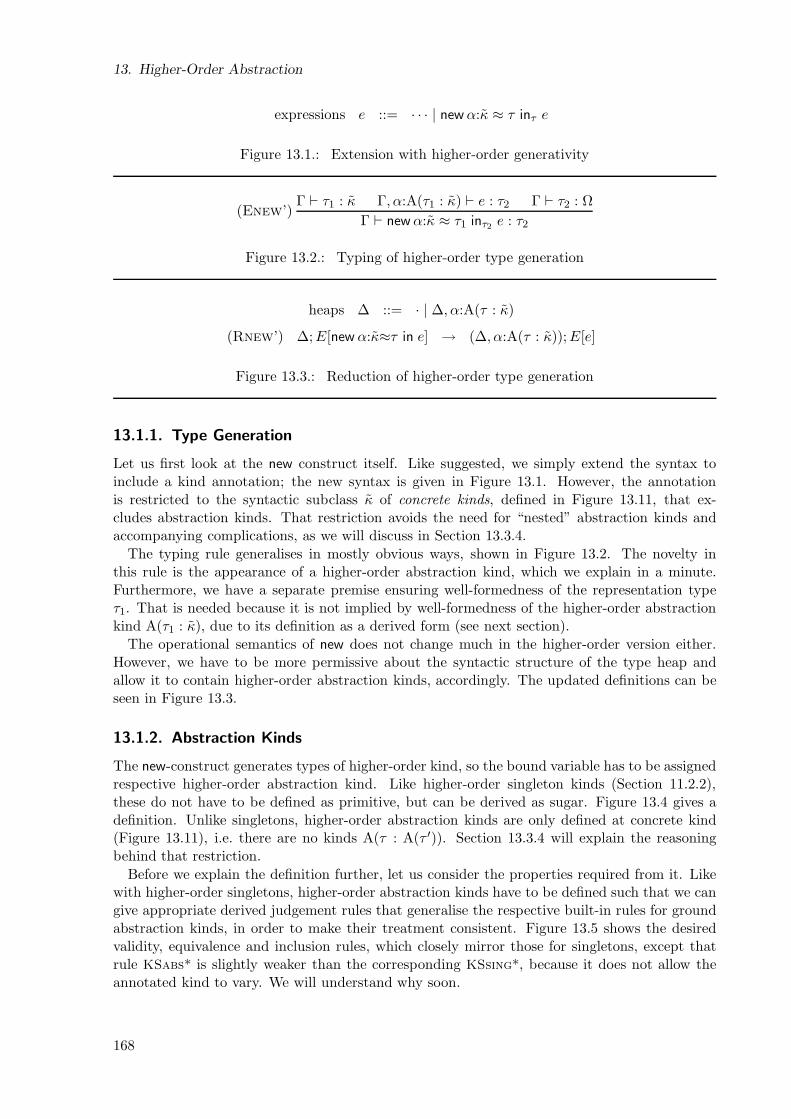
13. Higher-Order Abstraction
expressions e ::= · · · | newα:κ ≈ τ inτ e
Figure 13.1.: Extension with higher-order generativity
(Enew’)Γ ⊢ τ1 : κ Γ, α:A(τ1 : κ) ⊢ e : τ2 Γ ⊢ τ2 : Ω
Γ ⊢ newα:κ ≈ τ1 inτ2 e : τ2
Figure 13.2.: Typing of higher-order type generation
heaps ∆ ::= · | ∆, α:A(τ : κ)
(Rnew’) ∆;E[new α:κ≈τ in e] → (∆, α:A(τ : κ));E[e]
Figure 13.3.: Reduction of higher-order type generation
13.1.1. Type Generation
Let us first look at the new construct itself. Like suggested, we simply extend the syntax toinclude a kind annotation; the new syntax is given in Figure 13.1. However, the annotationis restricted to the syntactic subclass κ of concrete kinds, defined in Figure 13.11, that ex-cludes abstraction kinds. That restriction avoids the need for “nested” abstraction kinds andaccompanying complications, as we will discuss in Section 13.3.4.
The typing rule generalises in mostly obvious ways, shown in Figure 13.2. The novelty inthis rule is the appearance of a higher-order abstraction kind, which we explain in a minute.Furthermore, we have a separate premise ensuring well-formedness of the representation typeτ1. That is needed because it is not implied by well-formedness of the higher-order abstractionkind A(τ1 : κ), due to its definition as a derived form (see next section).
The operational semantics of new does not change much in the higher-order version either.However, we have to be more permissive about the syntactic structure of the type heap andallow it to contain higher-order abstraction kinds, accordingly. The updated definitions can beseen in Figure 13.3.
13.1.2. Abstraction Kinds
The new-construct generates types of higher-order kind, so the bound variable has to be assignedrespective higher-order abstraction kind. Like higher-order singleton kinds (Section 11.2.2),these do not have to be defined as primitive, but can be derived as sugar. Figure 13.4 gives adefinition. Unlike singletons, higher-order abstraction kinds are only defined at concrete kind(Figure 13.11), i.e. there are no kinds A(τ : A(τ ′)). Section 13.3.4 will explain the reasoningbehind that restriction.
Before we explain the definition further, let us consider the properties required from it. Likewith higher-order singletons, higher-order abstraction kinds have to be defined such that we cangive appropriate derived judgement rules that generalise the respective built-in rules for groundabstraction kinds, in order to make their treatment consistent. Figure 13.5 shows the desiredvalidity, equivalence and inclusion rules, which closely mirror those for singletons, except thatrule KSabs* is slightly weaker than the corresponding KSsing*, because it does not allow theannotated kind to vary. We will understand why soon.
168
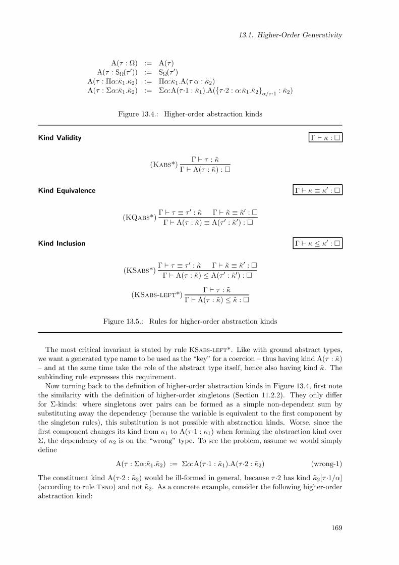
13.1. Higher-Order Generativity
A(τ : Ω) := A(τ)A(τ : SΩ(τ ′)) := SΩ(τ ′)
A(τ : Πα:κ1.κ2) := Πα:κ1.A(τ α : κ2)A(τ : Σα:κ1.κ2) := Σα:A(τ ·1 : κ1).A(τ ·2 : α:κ1.κ2α/τ ·1 : κ2)
Figure 13.4.: Higher-order abstraction kinds
Kind Validity Γ ⊢ κ :
(Kabs*)Γ ⊢ τ : κ
Γ ⊢ A(τ : κ) :
Kind Equivalence Γ ⊢ κ ≡ κ′ :
(KQabs*)Γ ⊢ τ ≡ τ ′ : κ Γ ⊢ κ ≡ κ′ :
Γ ⊢ A(τ : κ) ≡ A(τ ′ : κ′) :
Kind Inclusion Γ ⊢ κ ≤ κ′ :
(KSabs*)Γ ⊢ τ ≡ τ ′ : κ Γ ⊢ κ ≡ κ′ :
Γ ⊢ A(τ : κ) ≤ A(τ ′ : κ′) :
(KSabs-left*)Γ ⊢ τ : κ
Γ ⊢ A(τ : κ) ≤ κ :
Figure 13.5.: Rules for higher-order abstraction kinds
The most critical invariant is stated by rule KSabs-left*. Like with ground abstract types,we want a generated type name to be used as the “key” for a coercion – thus having kind A(τ : κ)– and at the same time take the role of the abstract type itself, hence also having kind κ. Thesubkinding rule expresses this requirement.
Now turning back to the definition of higher-order abstraction kinds in Figure 13.4, first notethe similarity with the definition of higher-order singletons (Section 11.2.2). They only differfor Σ-kinds: where singletons over pairs can be formed as a simple non-dependent sum bysubstituting away the dependency (because the variable is equivalent to the first component bythe singleton rules), this substitution is not possible with abstraction kinds. Worse, since thefirst component changes its kind from κ1 to A(τ ·1 : κ1) when forming the abstraction kind overΣ, the dependency of κ2 is on the “wrong” type. To see the problem, assume we would simplydefine
A(τ : Σα:κ1.κ2) := Σα:A(τ ·1 : κ1).A(τ ·2 : κ2) (wrong-1)
The constituent kind A(τ ·2 : κ2) would be ill-formed in general, because τ ·2 has kind κ2[τ ·1/α](according to rule Tsnd) and not κ2. As a concrete example, consider the following higher-orderabstraction kind:
169
13. Higher-Order Abstraction
κ = A(τ : Σα:Ω.SΩ(α) → Ω) with τ = 〈int , λβ:SΩ(int).β〉
It roughly corresponds to the following use of sealing in ML:
struct type t = int; functor F (type u = int) = (type v = u) end
:> sig type t; functor F (type u = t) : (type v) end
Assuming definition (wrong-1), κ would expand to
Σα:A(τ ·1).A(τ ·2 : SΩ(α) → Ω)
which further expands to
Σα:A(τ ·1).Πβ:SΩ(α).A(τ ·2β)
where the type application τ ·2β is ill-formed, because τ ·2 has argument kind SΩ(int), but β isof kind SΩ(α), and α 6≡ int .
On the other hand, defining
A(τ : Σα:κ1.κ2) := Σα:A(τ ·1 : κ1).A(τ ·2 : κ2[τ ·1/α]) (wrong-2)
would produce a well-formed expansion, but would also prevent A(τ : Σα:κ1.κ2) from being asubkind of the underlying kind Σα:κ1.κ2 – obviously, it would specialise only Σα:κ1.κ2[τ ·1/α].For our previous example, κ would become
Σα:A(τ ·1).A(τ ·2 : SΩ(int) → Ω)
Clearly, this cannot be a subkind of Σα:Ω.SΩ(α) → Ω, again because α 6≡ int . Consequently,definition (wrong-2) would break the essential rule KSabs-left*.
The expansion we actually need for κ is a kind that is equivalent to the following:
Σα:A(int).A(λβ:SΩ(α).β : SΩ(α) → Ω)
Here, instead of adapting the kind annotation in the second component, the critical occurrenceof int in τ ·2 has been “reverse-substituted” by α in the constitutent type, in order to matchthe original kind annotation. The expansion is well-formed and obeys the desired subkindingrelation. The kind coercion in Figure 13.4 achieves precisely this transformation and thus bridgesthe critical kind discrepancy.
We hence are left with developing kind coercions. However, kind coercions are somewhatintricate and likely to be more understandable once we have introduced the more earthly notionof type coercions. We thus delay the definition of kind coercions until Section 13.3.
Finally, note that well-formedness of a kind A(τ : κ) does not necessarily imply that τ : κ. Inparticular, in the case of κ = SΩ(τ ′) the expansion does not contain τ , so any judgement aboutA(τ : κ) is vacuous on τ . In contexts where a well-formed τ is needed that requirement has tobe stated separately. This is the same situation as with higher-order singletons [SH06].
13.1.3. Type Coercions
One interesting and nifty consequence of the fine-grained notion of abstraction kinds is that themove to higher-order generativity itself does not require any change to the concept of basic typecoercions: because we already allow the abstract type τ in a coercion e±τ to be representedby an arbitrary type expression, and because higher-order abstraction kinds simply decomposeinto ground ones, coercions already can express values of higher-order abstract type.
Consider an abstract type of stacks:
170
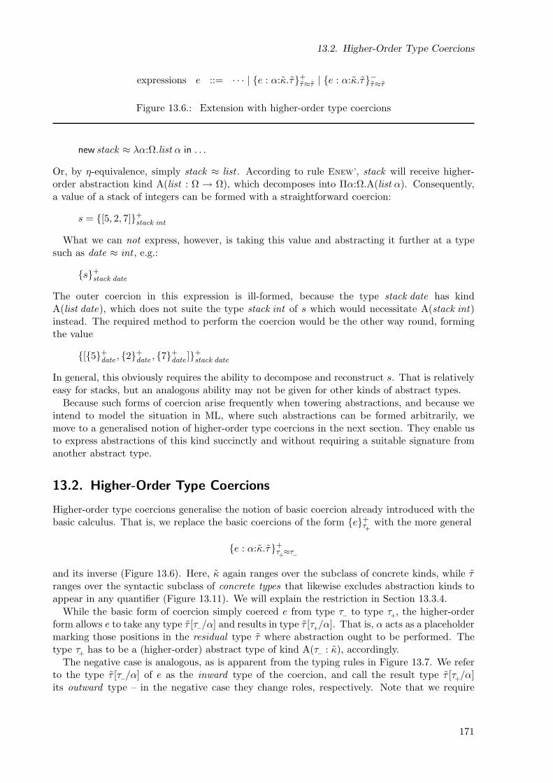
13.2. Higher-Order Type Coercions
expressions e ::= · · · | e : α:κ.τ+τ≈τ | e : α:κ.τ−τ≈τ
Figure 13.6.: Extension with higher-order type coercions
new stack ≈ λα:Ω.list α in . . .
Or, by η-equivalence, simply stack ≈ list . According to rule Enew’, stack will receive higher-order abstraction kind A(list : Ω → Ω), which decomposes into Πα:Ω.A(list α). Consequently,a value of a stack of integers can be formed with a straightforward coercion:
s = [5, 2, 7]+stack int
What we can not express, however, is taking this value and abstracting it further at a typesuch as date ≈ int , e.g.:
s+stack date
The outer coercion in this expression is ill-formed, because the type stack date has kindA(list date), which does not suite the type stack int of s which would necessitate A(stack int)instead. The required method to perform the coercion would be the other way round, formingthe value
[5+date
, 2+date
, 7+date
]+stack date
In general, this obviously requires the ability to decompose and reconstruct s. That is relativelyeasy for stacks, but an analogous ability may not be given for other kinds of abstract types.
Because such forms of coercion arise frequently when towering abstractions, and because weintend to model the situation in ML, where such abstractions can be formed arbitrarily, wemove to a generalised notion of higher-order type coercions in the next section. They enable usto express abstractions of this kind succinctly and without requiring a suitable signature fromanother abstract type.
13.2. Higher-Order Type Coercions
Higher-order type coercions generalise the notion of basic coercion already introduced with thebasic calculus. That is, we replace the basic coercions of the form e+
τ+
with the more general
e : α:κ.τ+τ+≈τ−
and its inverse (Figure 13.6). Here, κ again ranges over the subclass of concrete kinds, while τranges over the syntactic subclass of concrete types that likewise excludes abstraction kinds toappear in any quantifier (Figure 13.11). We will explain the restriction in Section 13.3.4.
While the basic form of coercion simply coerced e from type τ− to type τ+, the higher-order
form allows e to take any type τ [τ−/α] and results in type τ [τ+/α]. That is, α acts as a placeholder
marking those positions in the residual type τ where abstraction ought to be performed. Thetype τ
+has to be a (higher-order) abstract type of kind A(τ− : κ), accordingly.
The negative case is analogous, as is apparent from the typing rules in Figure 13.7. We referto the type τ [τ−/α] of e as the inward type of the coercion, and call the result type τ [τ
+/α]
its outward type – in the negative case they change roles, respectively. Note that we require
171
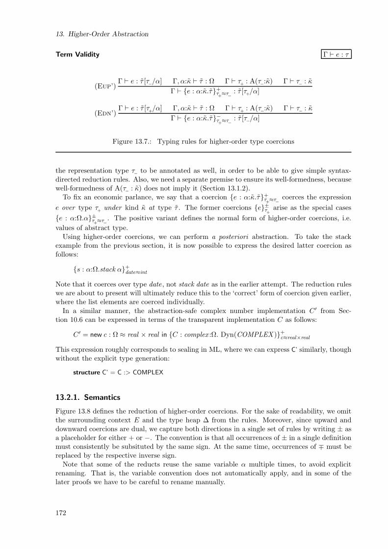
13. Higher-Order Abstraction
Term Validity Γ ⊢ e : τ
(Eup’)Γ ⊢ e : τ [τ−/α] Γ, α:κ ⊢ τ : Ω Γ ⊢ τ
+: A(τ−:κ) Γ ⊢ τ− : κ
Γ ⊢ e : α:κ.τ+τ+≈τ−
: τ [τ+/α]
(Edn’)Γ ⊢ e : τ [τ
+/α] Γ, α:κ ⊢ τ : Ω Γ ⊢ τ
+: A(τ−:κ) Γ ⊢ τ− : κ
Γ ⊢ e : α:κ.τ−τ+≈τ−
: τ [τ−/α]
Figure 13.7.: Typing rules for higher-order type coercions
the representation type τ− to be annotated as well, in order to be able to give simple syntax-directed reduction rules. Also, we need a separate premise to ensure its well-formedness, becausewell-formedness of A(τ− : κ) does not imply it (Section 13.1.2).
To fix an economic parlance, we say that a coercion e : α:κ.τ+τ+≈τ−
coerces the expression
e over type τ+
under kind κ at type τ . The former coercions e±τ+
arise as the special cases
e : α:Ω.α±τ+≈τ−
. The positive variant defines the normal form of higher-order coercions, i.e.
values of abstract type.
Using higher-order coercions, we can perform a posteriori abstraction. To take the stackexample from the previous section, it is now possible to express the desired latter coercion asfollows:
s : α:Ω.stack α+date≈int
Note that it coerces over type date , not stack date as in the earlier attempt. The reduction ruleswe are about to present will ultimately reduce this to the ‘correct’ form of coercion given earlier,where the list elements are coerced individually.
In a similar manner, the abstraction-safe complex number implementation C ′ from Sec-tion 10.6 can be expressed in terms of the transparent implementation C as follows:
C ′ = new c : Ω ≈ real × real in C : complex :Ω. Dyn(COMPLEX )+c≈real×real
This expression roughly corresponds to sealing in ML, where we can express C’ similarly, thoughwithout the explicit type generation:
structure C’ = C :> COMPLEX
13.2.1. Semantics
Figure 13.8 defines the reduction of higher-order coercions. For the sake of readability, we omitthe surrounding context E and the type heap ∆ from the rules. Moreover, since upward anddownward coercions are dual, we capture both directions in a single set of rules by writing ± asa placeholder for either + or −. The convention is that all occurrences of ± in a single definitionmust consistently be subsituted by the same sign. At the same time, occurrences of ∓ must bereplaced by the respective inverse sign.
Note that some of the reducts reuse the same variable α multiple times, to avoid explicitrenaming. That is, the variable convention does not automatically apply, and in some of thelater proofs we have to be careful to rename manually.
172
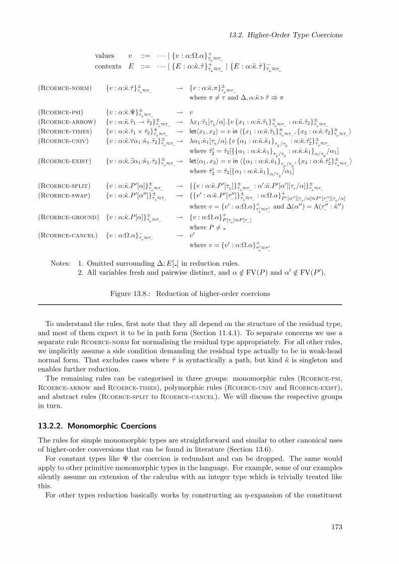
13.2. Higher-Order Type Coercions
values v ::= · · · | v : α:Ω.α+τ+≈τ−
contexts E ::= · · · | E : α:κ.τ+τ+≈τ−
| E : α:κ.τ−τ+≈τ−
(Rcoerce-norm) v : α:κ.τ±τ+≈τ
−→ v : α:κ.π±τ
+≈τ
−
where π 6= τ and ∆, α:κ ⊲ τ π
(Rcoerce-psi) v : α:κ.Ψ±τ+≈τ
−→ v
(Rcoerce-arrow) v : α:κ.τ1 → τ2±τ+≈τ−
→ λx1:τ1[τ±/α].v x1 : α:κ.τ1∓τ+≈τ−
: α:κ.τ2±τ+≈τ−
(Rcoerce-times) v : α:κ.τ1 × τ2±τ+≈τ−
→ let〈x1, x2〉 = v in 〈x1 : α:κ.τ1±τ+≈τ−
, x2 : α:κ.τ2±τ+≈τ−
〉
(Rcoerce-univ) v : α:κ.∀α1:κ1.τ2±τ+≈τ−
→ λα1:κ1[τ±/α].v α1 : α:κ.κ1τ∓/τ±: α:κ.τ ′2
±τ+≈τ−
where τ ′2 = τ2[α1 : α:κ.κ1τ∓
/τ±
: α:κ.κ1α/τ∓/α1]
(Rcoerce-exist) v : α:κ.∃α1:κ1.τ2±τ+≈τ−
→ let〈α1, x2〉 = v in 〈α1 : α:κ.κ1τ±
/τ∓, x2 : α:κ.τ ′2
±τ+≈τ−
〉
where τ ′2 = τ2[α1 : α:κ.κ1α/τ∓/α1]
(Rcoerce-split) v : α:κ.P ′[α]±τ+≈τ
−→ v : α:κ.P ′[τ∓]±τ
+≈τ
−: α′:κ.P ′[α′][τ
+/α]±τ
+≈τ
−
(Rcoerce-swap) v : α:κ.P ′[α′′]±τ+≈τ
−→ v′ : α:κ.P ′[τ ′′
−]±τ
+≈τ
−: α:Ω.α+
P ′[α′′][τ+
/α]≈P ′[τ ′′−
][τ+
/α]
where v = v′ : α:Ω.α+τ ′+≈τ ′
−and ∆(α′′) = A(τ ′′
−: κ′′)
(Rcoerce-ground) v : α:κ.P [α]±τ+≈τ
−→ v : α:Ω.α+
P [τ+]≈P [τ
−]
where P 6=(Rcoerce-cancel) v : α:Ω.α−τ
+≈τ−
→ v′
where v = v′ : α:Ω.α+τ ′+≈τ ′
−
Notes: 1. Omitted surrounding ∆;E[ ] in reduction rules.2. All variables fresh and pairwise distinct, and α /∈ FV(P ) and α′ /∈ FV(P ′).
Figure 13.8.: Reduction of higher-order coercions
To understand the rules, first note that they all depend on the structure of the residual type,and most of them expect it to be in path form (Section 11.4.1). To separate concerns we use aseparate rule Rcoerce-norm for normalising the residual type appropriately. For all other rules,we implicitly assume a side condition demanding the residual type actually to be in weak-headnormal form. That excludes cases where τ is syntactically a path, but kind κ is singleton andenables further reduction.
The remaining rules can be categorised in three groups: monomorphic rules (Rcoerce-psi,Rcoerce-arrow and Rcoerce-times), polymorphic rules (Rcoerce-univ and Rcoerce-exist),and abstract rules (Rcoerce-split to Rcoerce-cancel). We will discuss the respective groupsin turn.
13.2.2. Monomorphic Coercions
The rules for simple monomorphic types are straightforward and similar to other canonical usesof higher-order conversions that can be found in literature (Section 13.6).
For constant types like Ψ the coercion is redundant and can be dropped. The same wouldapply to other primitive monomorphic types in the language. For example, some of our examplessilently assume an extension of the calculus with an integer type which is trivially treated likethis.
For other types reduction basically works by constructing an η-expansion of the constituent
173
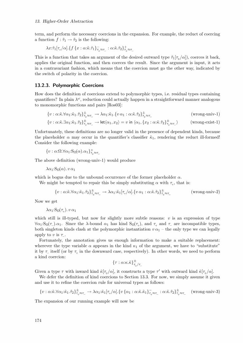
13. Higher-Order Abstraction
term, and perform the necessary coercions in the expansion. For example, the reduct of coercinga function f : τ1 → τ2 is the following:
λx:τ1[τ+/α].f x : α:κ.τ1−τ+≈τ−
: α:κ.τ2+τ+≈τ−
This is a function that takes an argument of the desired outward type τ1[τ±/α]), coerces it back,applies the original function, and then coerces the result. Since the argument is input, it actsin a contravariant fashion, which means that the coercion must go the other way, indicated bythe switch of polarity in the coercion.
13.2.3. Polymorphic Coercions
How does the definition of coercions extend to polymorphic types, i.e. residual types containingquantifiers? In plain λω, reduction could actually happen in a straightforward manner analogousto monomorphic functions and pairs [Ros03]:
v : α:κ.∀α1:κ1.τ2±τ+≈τ−
→ λα1:κ1.v α1 : α:κ.τ2±τ+≈τ−
(wrong-univ-1)
v : α:κ.∃α1:κ1.τ2±τ+≈τ−
→ let〈α1, x2〉 = v in 〈α1, x2 : α:κ.τ2±τ+≈τ−
〉 (wrong-exist-1)
Unfortunately, these definitions are no longer valid in the presence of dependent kinds, becausethe placeholder α may occur in the quantifier’s classifier κ1, rendering the reduct ill-formed!Consider the following example:
v : α:Ω.∀α1:SΩ(α).α1+τ+≈τ−
The above definition (wrong-univ-1) would produce
λα1:SΩ(α). v α1
which is bogus due to the unbound occurrence of the former placeholder α.We might be tempted to repair this be simply substituting α with τ
+, that is:
v : α:κ.∀α1:κ1.τ2±τ+≈τ−
→ λα1:κ1[τ+/α].v α1 : α:κ.τ2±τ+≈τ−
(wrong-univ-2)
Now we get
λα1:SΩ(τ+). v α1
which still is ill-typed, but now for slightly more subtle reasons: v is an expression of type∀α1:SΩ(τ−).α1. Since the λ-bound α1 has kind SΩ(τ
+), and τ
+and τ− are incompatible types,
both singleton kinds clash at the polymorphic instantiation v α1 – the only type we can legallyapply to v is τ−.
Fortunately, the annotation gives us enough information to make a suitable replacement:wherever the type variable α appears in the kind κ1 of the argument, we have to “substitute”it by τ− itself (or by τ
+in the downward case, respectively). In other words, we need to perform
a kind coercion:τ : α:κ.κ±τ
+/τ−
Given a type τ with inward kind κ[τ∓/α], it constructs a type τ ′ with outward kind κ[τ±/α].We defer the definition of kind coercions to Section 13.3. For now, we simply assume it given
and use it to refine the coercion rule for universal types as follows:
v : α:κ.∀α1:κ1.τ2±τ+≈τ−
→ λα1:κ1[τ+/α].v α1 : α:κ.κ1−τ+≈τ−
: α:κ.τ2±τ+≈τ−
(wrong-univ-3)
The expansion of our running example will now be
174
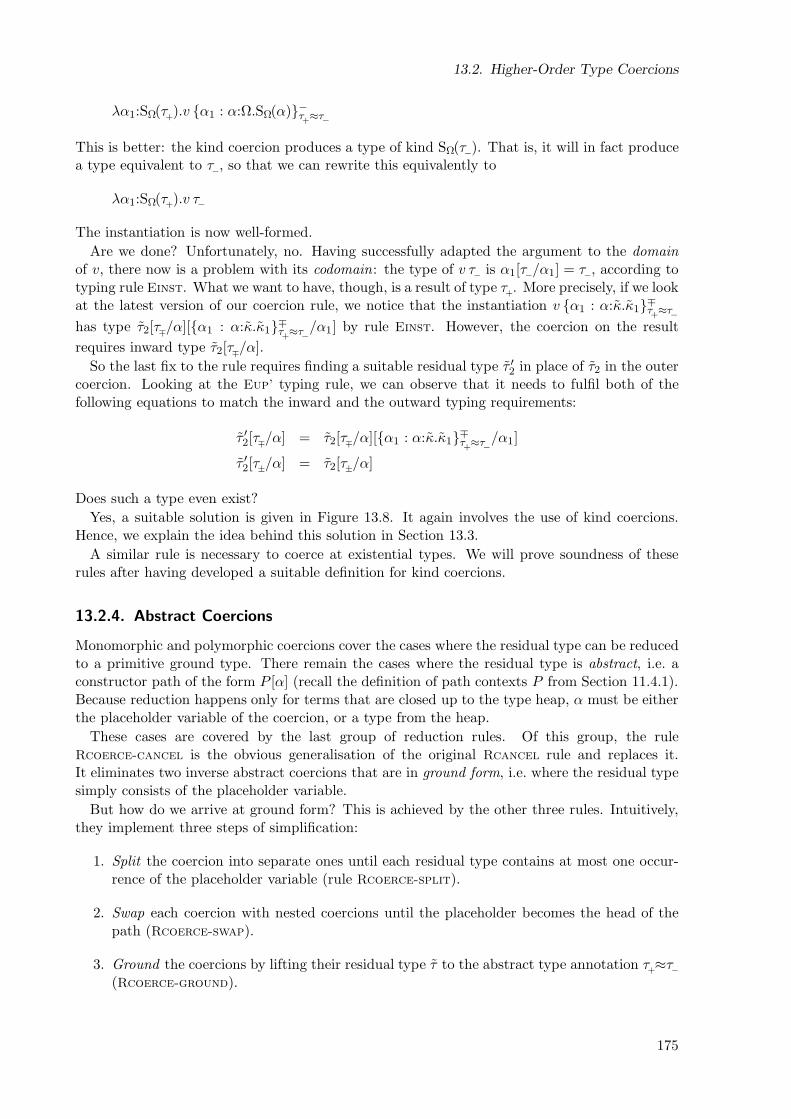
13.2. Higher-Order Type Coercions
λα1:SΩ(τ+).v α1 : α:Ω.SΩ(α)−τ
+≈τ−
This is better: the kind coercion produces a type of kind SΩ(τ−). That is, it will in fact producea type equivalent to τ−, so that we can rewrite this equivalently to
λα1:SΩ(τ+).v τ−
The instantiation is now well-formed.
Are we done? Unfortunately, no. Having successfully adapted the argument to the domainof v, there now is a problem with its codomain: the type of v τ− is α1[τ−/α1] = τ−, according totyping rule Einst. What we want to have, though, is a result of type τ
+. More precisely, if we look
at the latest version of our coercion rule, we notice that the instantiation v α1 : α:κ.κ1∓τ+≈τ−
has type τ2[τ∓/α][α1 : α:κ.κ1∓τ+≈τ−
/α1] by rule Einst. However, the coercion on the result
requires inward type τ2[τ∓/α].
So the last fix to the rule requires finding a suitable residual type τ ′2 in place of τ2 in the outercoercion. Looking at the Eup’ typing rule, we can observe that it needs to fulfil both of thefollowing equations to match the inward and the outward typing requirements:
τ ′2[τ∓/α] = τ2[τ∓/α][α1 : α:κ.κ1∓τ+≈τ−
/α1]
τ ′2[τ±/α] = τ2[τ±/α]
Does such a type even exist?
Yes, a suitable solution is given in Figure 13.8. It again involves the use of kind coercions.Hence, we explain the idea behind this solution in Section 13.3.
A similar rule is necessary to coerce at existential types. We will prove soundness of theserules after having developed a suitable definition for kind coercions.
13.2.4. Abstract Coercions
Monomorphic and polymorphic coercions cover the cases where the residual type can be reducedto a primitive ground type. There remain the cases where the residual type is abstract, i.e. aconstructor path of the form P [α] (recall the definition of path contexts P from Section 11.4.1).Because reduction happens only for terms that are closed up to the type heap, α must be eitherthe placeholder variable of the coercion, or a type from the heap.
These cases are covered by the last group of reduction rules. Of this group, the ruleRcoerce-cancel is the obvious generalisation of the original Rcancel rule and replaces it.It eliminates two inverse abstract coercions that are in ground form, i.e. where the residual typesimply consists of the placeholder variable.
But how do we arrive at ground form? This is achieved by the other three rules. Intuitively,they implement three steps of simplification:
1. Split the coercion into separate ones until each residual type contains at most one occur-rence of the placeholder variable (rule Rcoerce-split).
2. Swap each coercion with nested coercions until the placeholder becomes the head of thepath (Rcoerce-swap).
3. Ground the coercions by lifting their residual type τ to the abstract type annotation τ+≈τ−
(Rcoerce-ground).
175
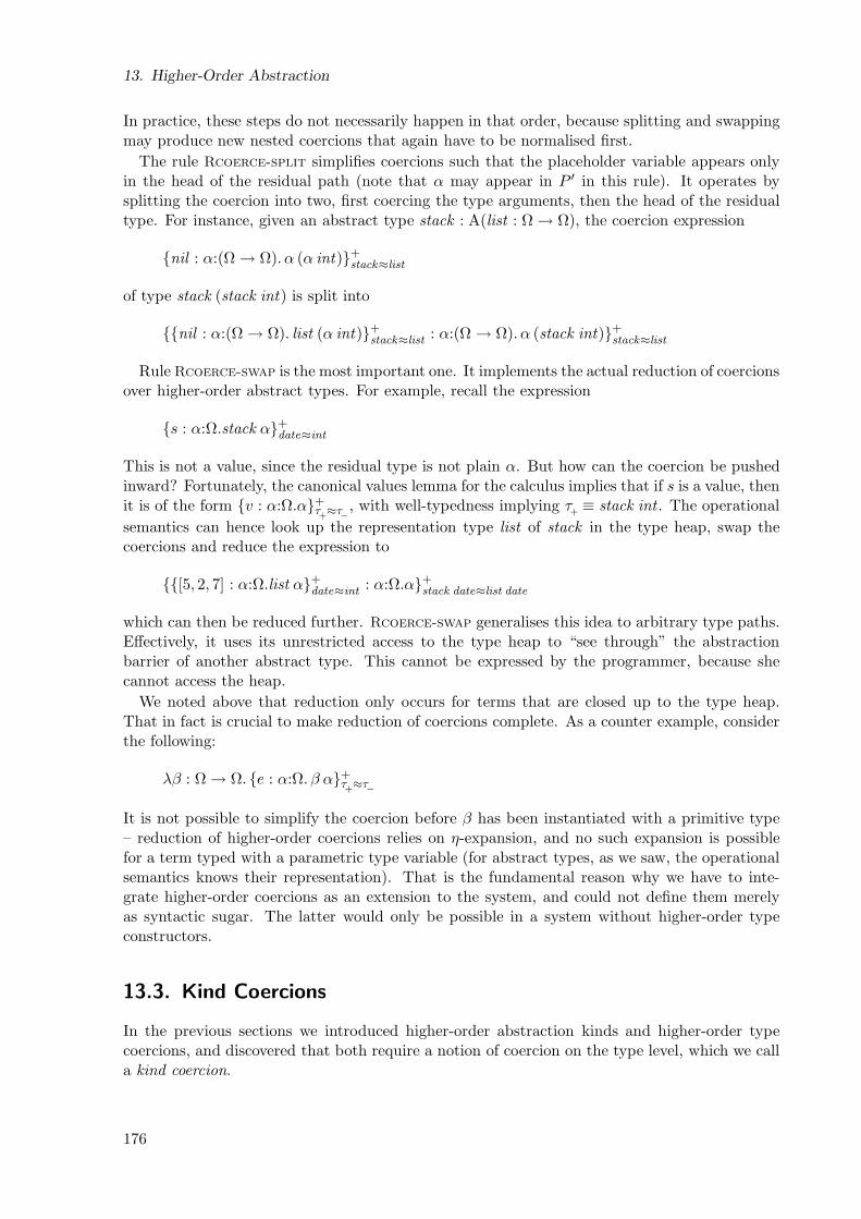
13. Higher-Order Abstraction
In practice, these steps do not necessarily happen in that order, because splitting and swappingmay produce new nested coercions that again have to be normalised first.
The rule Rcoerce-split simplifies coercions such that the placeholder variable appears onlyin the head of the residual path (note that α may appear in P ′ in this rule). It operates bysplitting the coercion into two, first coercing the type arguments, then the head of the residualtype. For instance, given an abstract type stack : A(list : Ω → Ω), the coercion expression
nil : α:(Ω → Ω). α (α int)+stack≈list
of type stack (stack int) is split into
nil : α:(Ω → Ω). list (α int)+stack≈list
: α:(Ω → Ω). α (stack int)+stack≈list
Rule Rcoerce-swap is the most important one. It implements the actual reduction of coercionsover higher-order abstract types. For example, recall the expression
s : α:Ω.stack α+date≈int
This is not a value, since the residual type is not plain α. But how can the coercion be pushedinward? Fortunately, the canonical values lemma for the calculus implies that if s is a value, thenit is of the form v : α:Ω.α+
τ+≈τ−
, with well-typedness implying τ+≡ stack int . The operational
semantics can hence look up the representation type list of stack in the type heap, swap thecoercions and reduce the expression to
[5, 2, 7] : α:Ω.list α+date≈int
: α:Ω.α+stack date≈list date
which can then be reduced further. Rcoerce-swap generalises this idea to arbitrary type paths.Effectively, it uses its unrestricted access to the type heap to “see through” the abstractionbarrier of another abstract type. This cannot be expressed by the programmer, because shecannot access the heap.
We noted above that reduction only occurs for terms that are closed up to the type heap.That in fact is crucial to make reduction of coercions complete. As a counter example, considerthe following:
λβ : Ω → Ω. e : α:Ω. β α+τ+≈τ−
It is not possible to simplify the coercion before β has been instantiated with a primitive type– reduction of higher-order coercions relies on η-expansion, and no such expansion is possiblefor a term typed with a parametric type variable (for abstract types, as we saw, the operationalsemantics knows their representation). That is the fundamental reason why we have to inte-grate higher-order coercions as an extension to the system, and could not define them merelyas syntactic sugar. The latter would only be possible in a system without higher-order typeconstructors.
13.3. Kind Coercions
In the previous sections we introduced higher-order abstraction kinds and higher-order typecoercions, and discovered that both require a notion of coercion on the type level, which we calla kind coercion.
176
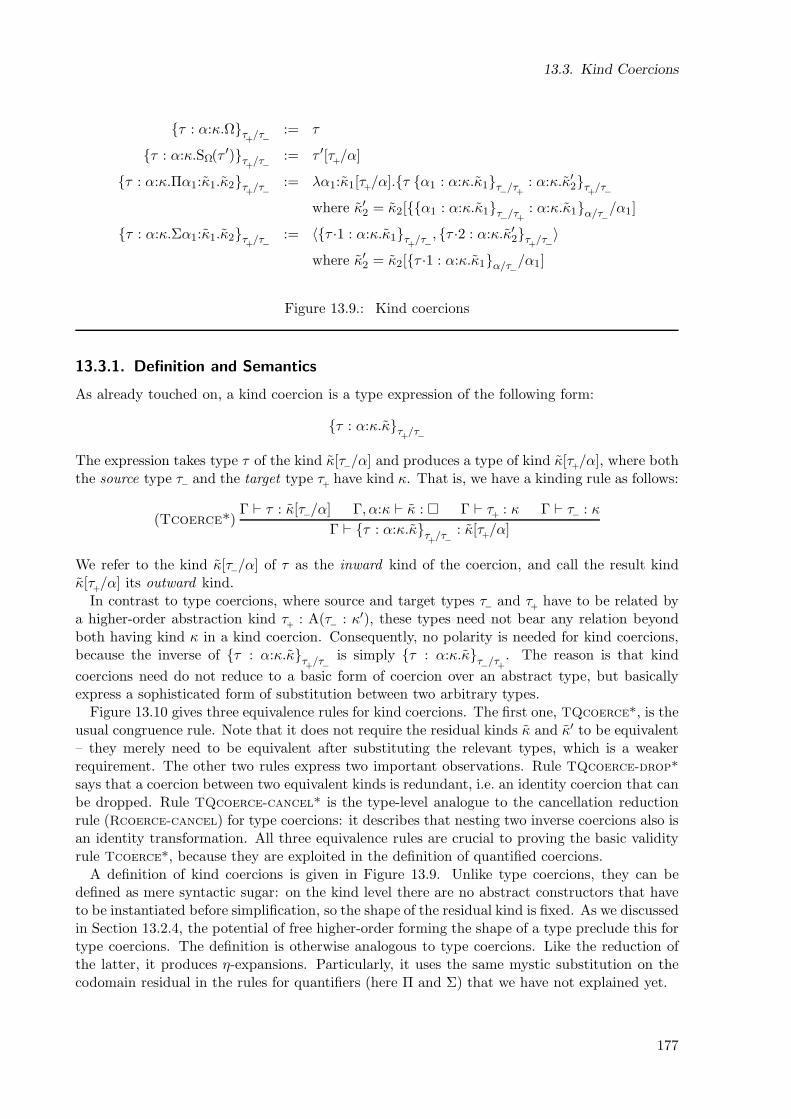
13.3. Kind Coercions
τ : α:κ.Ωτ+
/τ−:= τ
τ : α:κ.SΩ(τ ′)τ+
/τ−:= τ ′[τ
+/α]
τ : α:κ.Πα1:κ1.κ2τ+
/τ−:= λα1:κ1[τ+/α].τ α1 : α:κ.κ1τ−/τ
+: α:κ.κ′2τ
+/τ−
where κ′2 = κ2[α1 : α:κ.κ1τ−/τ+
: α:κ.κ1α/τ−/α1]
τ : α:κ.Σα1:κ1.κ2τ+
/τ−:= 〈τ ·1 : α:κ.κ1τ
+/τ−, τ ·2 : α:κ.κ′2τ
+/τ−
〉
where κ′2 = κ2[τ ·1 : α:κ.κ1α/τ−/α1]
Figure 13.9.: Kind coercions
13.3.1. Definition and Semantics
As already touched on, a kind coercion is a type expression of the following form:
τ : α:κ.κτ+
/τ−
The expression takes type τ of the kind κ[τ−/α] and produces a type of kind κ[τ+/α], where both
the source type τ− and the target type τ+
have kind κ. That is, we have a kinding rule as follows:
(Tcoerce*)Γ ⊢ τ : κ[τ−/α] Γ, α:κ ⊢ κ : Γ ⊢ τ
+: κ Γ ⊢ τ− : κ
Γ ⊢ τ : α:κ.κτ+
/τ−: κ[τ
+/α]
We refer to the kind κ[τ−/α] of τ as the inward kind of the coercion, and call the result kindκ[τ
+/α] its outward kind.
In contrast to type coercions, where source and target types τ− and τ+
have to be related bya higher-order abstraction kind τ
+: A(τ− : κ′), these types need not bear any relation beyond
both having kind κ in a kind coercion. Consequently, no polarity is needed for kind coercions,because the inverse of τ : α:κ.κτ
+/τ−
is simply τ : α:κ.κτ−/τ+
. The reason is that kind
coercions need do not reduce to a basic form of coercion over an abstract type, but basicallyexpress a sophisticated form of substitution between two arbitrary types.
Figure 13.10 gives three equivalence rules for kind coercions. The first one, TQcoerce*, is theusual congruence rule. Note that it does not require the residual kinds κ and κ′ to be equivalent– they merely need to be equivalent after substituting the relevant types, which is a weakerrequirement. The other two rules express two important observations. Rule TQcoerce-drop*
says that a coercion between two equivalent kinds is redundant, i.e. an identity coercion that canbe dropped. Rule TQcoerce-cancel* is the type-level analogue to the cancellation reductionrule (Rcoerce-cancel) for type coercions: it describes that nesting two inverse coercions also isan identity transformation. All three equivalence rules are crucial to proving the basic validityrule Tcoerce*, because they are exploited in the definition of quantified coercions.
A definition of kind coercions is given in Figure 13.9. Unlike type coercions, they can bedefined as mere syntactic sugar: on the kind level there are no abstract constructors that haveto be instantiated before simplification, so the shape of the residual kind is fixed. As we discussedin Section 13.2.4, the potential of free higher-order forming the shape of a type preclude this fortype coercions. The definition is otherwise analogous to type coercions. Like the reduction ofthe latter, it produces η-expansions. Particularly, it uses the same mystic substitution on thecodomain residual in the rules for quantifiers (here Π and Σ) that we have not explained yet.
177
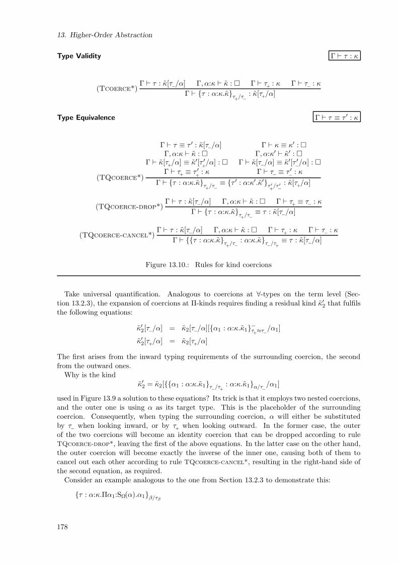
13. Higher-Order Abstraction
Type Validity Γ ⊢ τ : κ
(Tcoerce*)Γ ⊢ τ : κ[τ−/α] Γ, α:κ ⊢ κ : Γ ⊢ τ
+: κ Γ ⊢ τ− : κ
Γ ⊢ τ : α:κ.κτ+
/τ−: κ[τ
+/α]
Type Equivalence Γ ⊢ τ ≡ τ ′ : κ
(TQcoerce*)
Γ ⊢ τ ≡ τ ′ : κ[τ−/α] Γ ⊢ κ ≡ κ′ : Γ, α:κ ⊢ κ : Γ, α:κ′ ⊢ κ′ :
Γ ⊢ κ[τ+/α] ≡ κ′[τ ′
+/α] : Γ ⊢ κ[τ−/α] ≡ κ′[τ ′
−/α] :
Γ ⊢ τ+≡ τ ′
+: κ Γ ⊢ τ− ≡ τ ′
−: κ
Γ ⊢ τ : α:κ.κτ+
/τ−≡ τ ′ : α:κ′.κ′τ ′
+/τ ′
−
: κ[τ+/α]
(TQcoerce-drop*)Γ ⊢ τ : κ[τ−/α] Γ, α:κ ⊢ κ : Γ ⊢ τ
+≡ τ− : κ
Γ ⊢ τ : α:κ.κτ+
/τ−≡ τ : κ[τ−/α]
(TQcoerce-cancel*)Γ ⊢ τ : κ[τ−/α] Γ, α:κ ⊢ κ : Γ ⊢ τ
+: κ Γ ⊢ τ− : κ
Γ ⊢ τ : α:κ.κτ+
/τ−: α:κ.κτ−/τ
+
≡ τ : κ[τ−/α]
Figure 13.10.: Rules for kind coercions
Take universal quantification. Analogous to coercions at ∀-types on the term level (Sec-tion 13.2.3), the expansion of coercions at Π-kinds requires finding a residual kind κ′2 that fulfilsthe following equations:
κ′2[τ−/α] = κ2[τ−/α][α1 : α:κ.κ1−τ+≈τ−
/α1]
κ′2[τ+/α] = κ2[τ+/α]
The first arises from the inward typing requirements of the surrounding coercion, the secondfrom the outward ones.
Why is the kindκ′2 = κ2[α1 : α:κ.κ1τ−/τ
+: α:κ.κ1α/τ−
/α1]
used in Figure 13.9 a solution to these equations? Its trick is that it employs two nested coercions,and the outer one is using α as its target type. This is the placeholder of the surroundingcoercion. Consequently, when typing the surrounding coercion, α will either be substitutedby τ− when looking inward, or by τ
+when looking outward. In the former case, the outer
of the two coercions will become an identity coercion that can be dropped according to ruleTQcoerce-drop*, leaving the first of the above equations. In the latter case on the other hand,the outer coercion will become exactly the inverse of the inner one, causing both of them tocancel out each other according to rule TQcoerce-cancel*, resulting in the right-hand side ofthe second equation, as required.
Consider an example analogous to the one from Section 13.2.3 to demonstrate this:
τ : α:κ.Πα1:SΩ(α).α1β/τβ
178
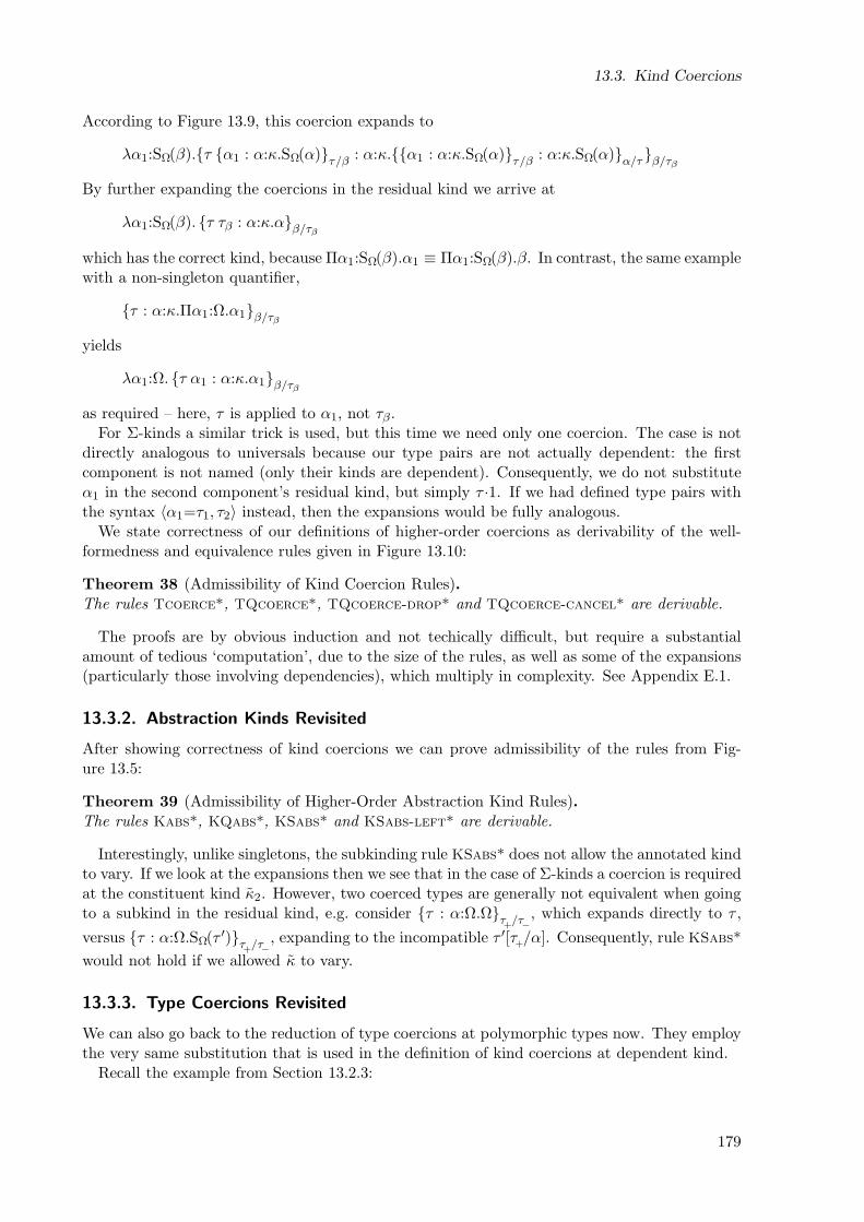
13.3. Kind Coercions
According to Figure 13.9, this coercion expands to
λα1:SΩ(β).τ α1 : α:κ.SΩ(α)τ/β : α:κ.α1 : α:κ.SΩ(α)τ/β : α:κ.SΩ(α)α/τβ/τβ
By further expanding the coercions in the residual kind we arrive at
λα1:SΩ(β). τ τβ : α:κ.αβ/τβ
which has the correct kind, because Πα1:SΩ(β).α1 ≡ Πα1:SΩ(β).β. In contrast, the same examplewith a non-singleton quantifier,
τ : α:κ.Πα1:Ω.α1β/τβ
yields
λα1:Ω. τ α1 : α:κ.α1β/τβ
as required – here, τ is applied to α1, not τβ.For Σ-kinds a similar trick is used, but this time we need only one coercion. The case is not
directly analogous to universals because our type pairs are not actually dependent: the firstcomponent is not named (only their kinds are dependent). Consequently, we do not substituteα1 in the second component’s residual kind, but simply τ ·1. If we had defined type pairs withthe syntax 〈α1=τ1, τ2〉 instead, then the expansions would be fully analogous.
We state correctness of our definitions of higher-order coercions as derivability of the well-formedness and equivalence rules given in Figure 13.10:
Theorem 38 (Admissibility of Kind Coercion Rules).The rules Tcoerce*, TQcoerce*, TQcoerce-drop* and TQcoerce-cancel* are derivable.
The proofs are by obvious induction and not techically difficult, but require a substantialamount of tedious ‘computation’, due to the size of the rules, as well as some of the expansions(particularly those involving dependencies), which multiply in complexity. See Appendix E.1.
13.3.2. Abstraction Kinds Revisited
After showing correctness of kind coercions we can prove admissibility of the rules from Fig-ure 13.5:
Theorem 39 (Admissibility of Higher-Order Abstraction Kind Rules).The rules Kabs*, KQabs*, KSabs* and KSabs-left* are derivable.
Interestingly, unlike singletons, the subkinding rule KSabs* does not allow the annotated kindto vary. If we look at the expansions then we see that in the case of Σ-kinds a coercion is requiredat the constituent kind κ2. However, two coerced types are generally not equivalent when goingto a subkind in the residual kind, e.g. consider τ : α:Ω.Ωτ
+/τ−
, which expands directly to τ ,
versus τ : α:Ω.SΩ(τ ′)τ+
/τ−, expanding to the incompatible τ ′[τ
+/α]. Consequently, rule KSabs*
would not hold if we allowed κ to vary.
13.3.3. Type Coercions Revisited
We can also go back to the reduction of type coercions at polymorphic types now. They employthe very same substitution that is used in the definition of kind coercions at dependent kind.
Recall the example from Section 13.2.3:
179
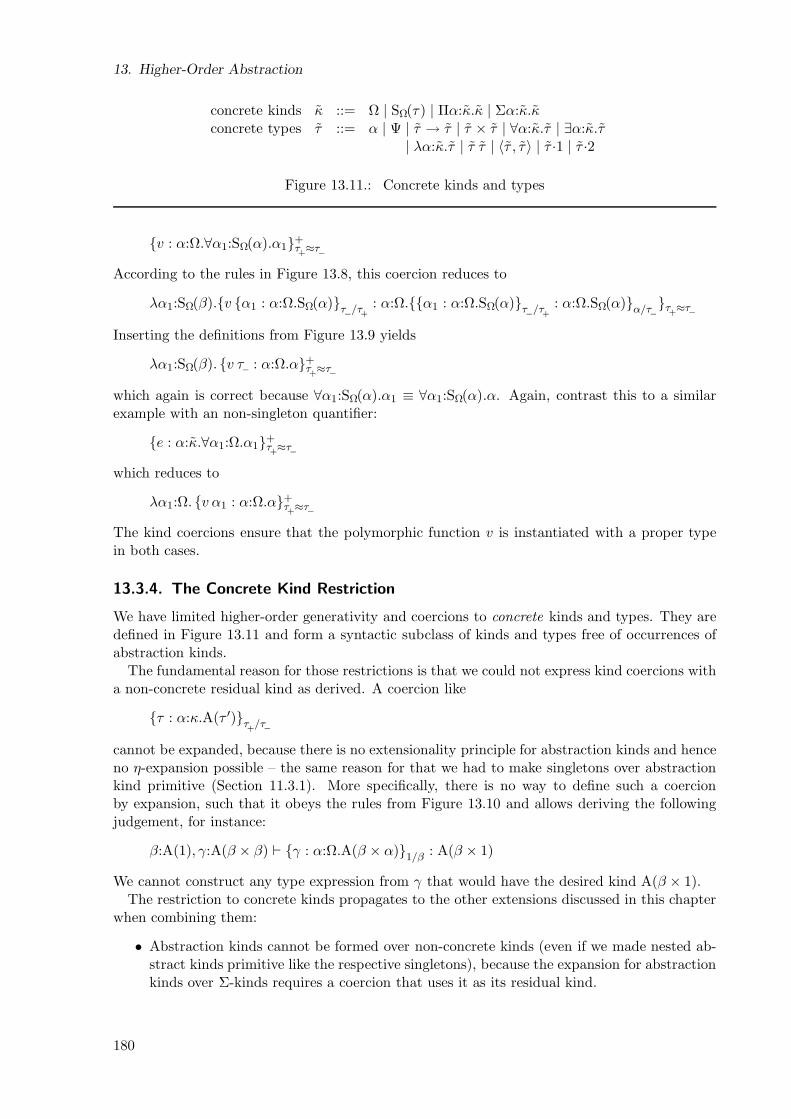
13. Higher-Order Abstraction
concrete kinds κ ::= Ω | SΩ(τ) | Πα:κ.κ | Σα:κ.κconcrete types τ ::= α | Ψ | τ → τ | τ × τ | ∀α:κ.τ | ∃α:κ.τ
| λα:κ.τ | τ τ | 〈τ , τ〉 | τ ·1 | τ ·2
Figure 13.11.: Concrete kinds and types
v : α:Ω.∀α1:SΩ(α).α1+τ+≈τ−
According to the rules in Figure 13.8, this coercion reduces to
λα1:SΩ(β).v α1 : α:Ω.SΩ(α)τ−/τ+
: α:Ω.α1 : α:Ω.SΩ(α)τ−/τ+
: α:Ω.SΩ(α)α/τ−τ
+≈τ−
Inserting the definitions from Figure 13.9 yields
λα1:SΩ(β). v τ− : α:Ω.α+τ+≈τ−
which again is correct because ∀α1:SΩ(α).α1 ≡ ∀α1:SΩ(α).α. Again, contrast this to a similarexample with an non-singleton quantifier:
e : α:κ.∀α1:Ω.α1+τ+≈τ−
which reduces to
λα1:Ω. v α1 : α:Ω.α+τ+≈τ−
The kind coercions ensure that the polymorphic function v is instantiated with a proper typein both cases.
13.3.4. The Concrete Kind Restriction
We have limited higher-order generativity and coercions to concrete kinds and types. They aredefined in Figure 13.11 and form a syntactic subclass of kinds and types free of occurrences ofabstraction kinds.
The fundamental reason for those restrictions is that we could not express kind coercions witha non-concrete residual kind as derived. A coercion like
τ : α:κ.A(τ ′)τ+
/τ−
cannot be expanded, because there is no extensionality principle for abstraction kinds and henceno η-expansion possible – the same reason for that we had to make singletons over abstractionkind primitive (Section 11.3.1). More specifically, there is no way to define such a coercionby expansion, such that it obeys the rules from Figure 13.10 and allows deriving the followingjudgement, for instance:
β:A(1), γ:A(β × β) ⊢ γ : α:Ω.A(β × α)1/β : A(β × 1)
We cannot construct any type expression from γ that would have the desired kind A(β × 1).The restriction to concrete kinds propagates to the other extensions discussed in this chapter
when combining them:
• Abstraction kinds cannot be formed over non-concrete kinds (even if we made nested ab-stract kinds primitive like the respective singletons), because the expansion for abstractionkinds over Σ-kinds requires a coercion that uses it as its residual kind.
180
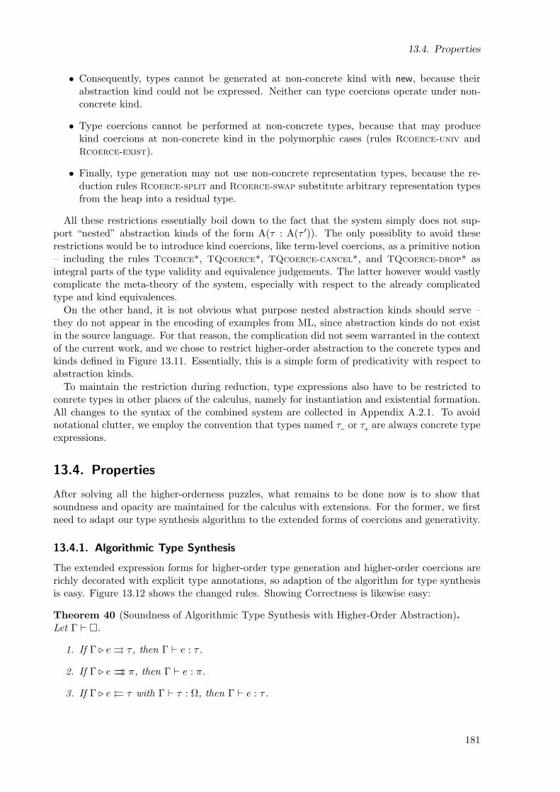
13.4. Properties
• Consequently, types cannot be generated at non-concrete kind with new, because theirabstraction kind could not be expressed. Neither can type coercions operate under non-concrete kind.
• Type coercions cannot be performed at non-concrete types, because that may producekind coercions at non-concrete kind in the polymorphic cases (rules Rcoerce-univ andRcoerce-exist).
• Finally, type generation may not use non-concrete representation types, because the re-duction rules Rcoerce-split and Rcoerce-swap substitute arbitrary representation typesfrom the heap into a residual type.
All these restrictions essentially boil down to the fact that the system simply does not sup-port “nested” abstraction kinds of the form A(τ : A(τ ′)). The only possiblity to avoid theserestrictions would be to introduce kind coercions, like term-level coercions, as a primitive notion– including the rules Tcoerce*, TQcoerce*, TQcoerce-cancel*, and TQcoerce-drop* asintegral parts of the type validity and equivalence judgements. The latter however would vastlycomplicate the meta-theory of the system, especially with respect to the already complicatedtype and kind equivalences.
On the other hand, it is not obvious what purpose nested abstraction kinds should serve –they do not appear in the encoding of examples from ML, since abstraction kinds do not existin the source language. For that reason, the complication did not seem warranted in the contextof the current work, and we chose to restrict higher-order abstraction to the concrete types andkinds defined in Figure 13.11. Essentially, this is a simple form of predicativity with respect toabstraction kinds.
To maintain the restriction during reduction, type expressions also have to be restricted toconrete types in other places of the calculus, namely for instantiation and existential formation.All changes to the syntax of the combined system are collected in Appendix A.2.1. To avoidnotational clutter, we employ the convention that types named τ− or τ
+are always concrete type
expressions.
13.4. Properties
After solving all the higher-orderness puzzles, what remains to be done now is to show thatsoundness and opacity are maintained for the calculus with extensions. For the former, we firstneed to adapt our type synthesis algorithm to the extended forms of coercions and generativity.
13.4.1. Algorithmic Type Synthesis
The extended expression forms for higher-order type generation and higher-order coercions arerichly decorated with explicit type annotations, so adaption of the algorithm for type synthesisis easy. Figure 13.12 shows the changed rules. Showing Correctness is likewise easy:
Theorem 40 (Soundness of Algorithmic Type Synthesis with Higher-Order Abstraction).Let Γ ⊢ .
1. If Γ ⊲ e τ , then Γ ⊢ e : τ .
2. If Γ ⊲ e π, then Γ ⊢ e : π.
3. If Γ ⊲ e τ with Γ ⊢ τ : Ω, then Γ ⊢ e : τ .
181
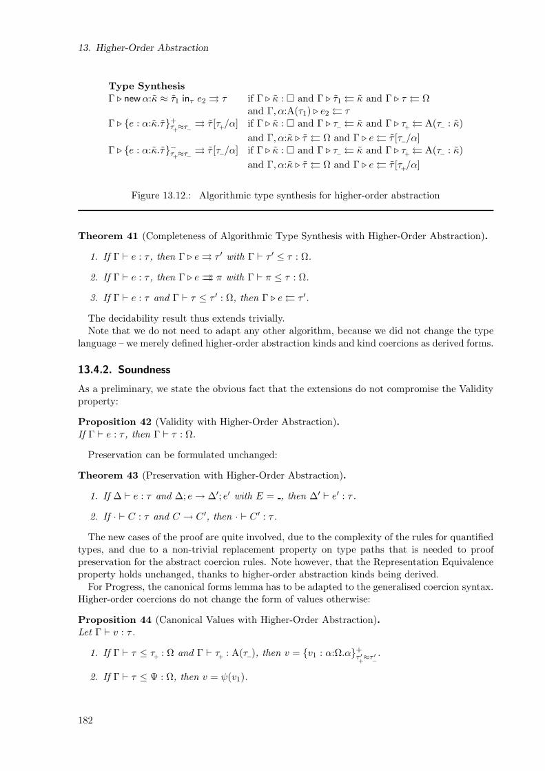
13. Higher-Order Abstraction
Type Synthesis
Γ ⊲ newα:κ ≈ τ1 inτ e2 τ if Γ ⊲ κ : and Γ ⊲ τ1 κ and Γ ⊲ τ Ωand Γ, α:A(τ1) ⊲ e2 τ
Γ ⊲ e : α:κ.τ+τ+≈τ− τ [τ
+/α] if Γ ⊲ κ : and Γ ⊲ τ− κ and Γ ⊲ τ
+ A(τ− : κ)
and Γ, α:κ ⊲ τ Ω and Γ ⊲ e τ [τ−/α]Γ ⊲ e : α:κ.τ−τ
+≈τ− τ [τ−/α] if Γ ⊲ κ : and Γ ⊲ τ− κ and Γ ⊲ τ
+ A(τ− : κ)
and Γ, α:κ ⊲ τ Ω and Γ ⊲ e τ [τ+/α]
Figure 13.12.: Algorithmic type synthesis for higher-order abstraction
Theorem 41 (Completeness of Algorithmic Type Synthesis with Higher-Order Abstraction).
1. If Γ ⊢ e : τ , then Γ ⊲ e τ ′ with Γ ⊢ τ ′ ≤ τ : Ω.
2. If Γ ⊢ e : τ , then Γ ⊲ e π with Γ ⊢ π ≤ τ : Ω.
3. If Γ ⊢ e : τ and Γ ⊢ τ ≤ τ ′ : Ω, then Γ ⊲ e τ ′.
The decidability result thus extends trivially.Note that we do not need to adapt any other algorithm, because we did not change the type
language – we merely defined higher-order abstraction kinds and kind coercions as derived forms.
13.4.2. Soundness
As a preliminary, we state the obvious fact that the extensions do not compromise the Validityproperty:
Proposition 42 (Validity with Higher-Order Abstraction).If Γ ⊢ e : τ , then Γ ⊢ τ : Ω.
Preservation can be formulated unchanged:
Theorem 43 (Preservation with Higher-Order Abstraction).
1. If ∆ ⊢ e : τ and ∆; e→ ∆′; e′ with E = , then ∆′ ⊢ e′ : τ .
2. If · ⊢ C : τ and C → C ′, then · ⊢ C ′ : τ .
The new cases of the proof are quite involved, due to the complexity of the rules for quantifiedtypes, and due to a non-trivial replacement property on type paths that is needed to proofpreservation for the abstract coercion rules. Note however, that the Representation Equivalenceproperty holds unchanged, thanks to higher-order abstraction kinds being derived.
For Progress, the canonical forms lemma has to be adapted to the generalised coercion syntax.Higher-order coercions do not change the form of values otherwise:
Proposition 44 (Canonical Values with Higher-Order Abstraction).Let Γ ⊢ v : τ .
1. If Γ ⊢ τ ≤ τ+
: Ω and Γ ⊢ τ+
: A(τ−), then v = v1 : α:Ω.α+τ ′+≈τ ′
−
.
2. If Γ ⊢ τ ≤ Ψ : Ω, then v = ψ(v1).
182
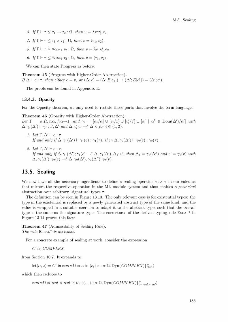
13.5. Sealing
3. If Γ ⊢ τ ≤ τ1 → τ2 : Ω, then v = λx:τ ′1.e2.
4. If Γ ⊢ τ ≤ τ1 × τ2 : Ω, then v = 〈v1, v2〉.
5. If Γ ⊢ τ ≤ ∀α:κ1.τ2 : Ω, then v = λα:κ′1.e2.
6. If Γ ⊢ τ ≤ ∃α:κ1.τ2 : Ω, then v = 〈τ1, v2〉.
We can then state Progress as before:
Theorem 45 (Progress with Higher-Order Abstraction).If ∆ ⊢ e : τ , then either e = v, or (∆; e) = (∆;E[e1]) → (∆′;E[e′1]) = (∆′; e′).
The proofs can be found in Appendix E.
13.4.3. Opacity
For the Opacity theorem, we only need to restate those parts that involve the term language:
Theorem 46 (Opacity with Higher-Order Abstraction).Let Γ = α:Ω, x:α, f :α→1, and γi = [αi/α] ∪ [vi/x] ∪ [v′i/f ] ∪ [α′ | α′ ∈ Dom(∆′)/α′] with∆, γi(∆
′) ⊢ γi : Γ,∆′ and ∆; v′i vi →∗ ∆; ⋄ for i ∈ 1, 2.
1. Let Γ,∆′ ⊢ e : τ .If and only if ∆, γ1(∆
′) ⊢ γ1(e) : γ1(τ), then ∆, γ2(∆′) ⊢ γ2(e) : γ2(τ).
2. Let Γ,∆′ ⊢ e : τ .If and only if ∆, γ1(∆
′); γ1(e) →∗ ∆, γ1(∆
′),∆1; v′, then ∆1 = γ1(∆
′′) and v′ = γ1(v) with∆, γ2(∆
′); γ2(e) →∗ ∆, γ2(∆
′), γ2(∆′′); γ2(v).
13.5. Sealing
We now have all the necessary ingredients to define a sealing operator e :> τ in our calculusthat mirrors the respective operation in the ML module system and thus enables a posterioriabstraction over arbitrary ‘signature’ types τ .
The definition can be seen in Figure 13.13. The only relevant case is for existential types: thetype in the existential is replaced by a newly generated abstract type of the same kind, and thevalue is wrapped in a suitable coercion to adapt it to the abstract type, such that the overalltype is the same as the signature type. The correctness of the derived typing rule Eseal* inFigure 13.14 proves this fact:
Theorem 47 (Admissibility of Sealing Rule).The rule Eseal* is derivable.
For a concrete example of sealing at work, consider the expression
C :> COMPLEX
from Section 10.7. It expands to
let〈α, x〉 = C ′ in new c:Ω ≈ α in 〈c, x : α:Ω.Dyn(COMPLEX )+c≈α〉
which then reduces to
new c:Ω ≈ real × real in 〈c, 〈. . .〉 : α:Ω.Dyn(COMPLEX )+c≈real×real
〉
183
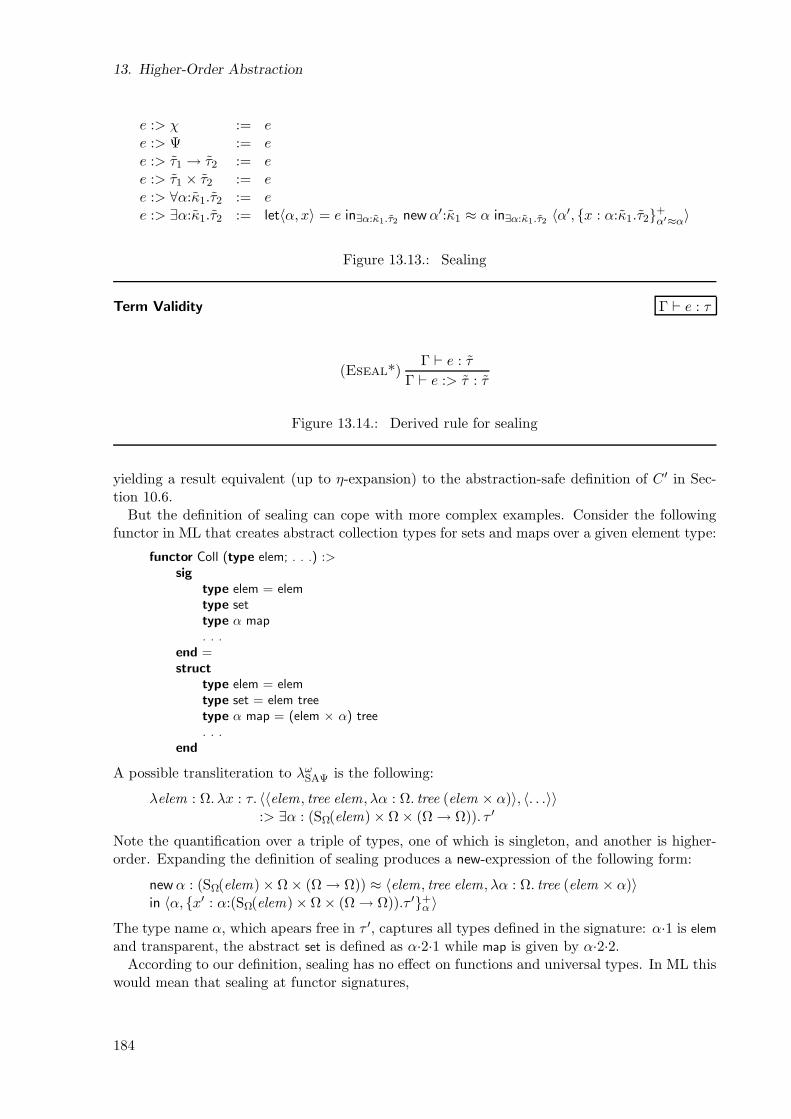
13. Higher-Order Abstraction
e :> χ := ee :> Ψ := ee :> τ1 → τ2 := ee :> τ1 × τ2 := ee :> ∀α:κ1.τ2 := ee :> ∃α:κ1.τ2 := let〈α, x〉 = e in∃α:κ1.τ2 newα′:κ1 ≈ α in∃α:κ1.τ2 〈α′, x : α:κ1.τ2
+α′≈α〉
Figure 13.13.: Sealing
Term Validity Γ ⊢ e : τ
(Eseal*)Γ ⊢ e : τ
Γ ⊢ e :> τ : τ
Figure 13.14.: Derived rule for sealing
yielding a result equivalent (up to η-expansion) to the abstraction-safe definition of C ′ in Sec-tion 10.6.
But the definition of sealing can cope with more complex examples. Consider the followingfunctor in ML that creates abstract collection types for sets and maps over a given element type:
functor Coll (type elem; . . .) :>sig
type elem = elemtype settype α map. . .
end =struct
type elem = elemtype set = elem treetype α map = (elem × α) tree. . .
end
A possible transliteration to λωSAΨ is the following:
λelem : Ω. λx : τ. 〈〈elem , tree elem, λα : Ω. tree (elem × α)〉, 〈. . .〉〉:> ∃α : (SΩ(elem) × Ω × (Ω → Ω)). τ ′
Note the quantification over a triple of types, one of which is singleton, and another is higher-order. Expanding the definition of sealing produces a new-expression of the following form:
newα : (SΩ(elem) × Ω × (Ω → Ω)) ≈ 〈elem, tree elem, λα : Ω. tree (elem × α)〉in 〈α, x′ : α:(SΩ(elem) × Ω × (Ω → Ω)).τ ′+
α 〉
The type name α, which apears free in τ ′, captures all types defined in the signature: α·1 is elem
and transparent, the abstract set is defined as α·2·1 while map is given by α·2·2.According to our definition, sealing has no effect on functions and universal types. In ML this
would mean that sealing at functor signatures,
184
13.6. Discussion and Related Work
F :> fct X : S1 → S2
does not have any effect. Less trivial semantics are possible, but would require giving a moreelaborate translation scheme for modules. In Appendix B we sketch such a scheme, but a morein-depth treatment is beyond the scope of this thesis.
Also note that for constructor types sealing has no effect either. This corresponds to the factthat in ML, signatures are not higher-order. In Alice ML, abstract signatures (Section 3.3.2) infact enable limited abstract sealing:
functor F (signature S) (X : S) = X :> S
Such an example would roughly correspond to sealing with a type variable in the calculus. If wewanted to have a semantics corresponding to Alice ML, it would be straightforward to realiseby making sealing primitive and turning the syntactic definition into reduction rules. However,since this feature is of little practical utility and does not provide any new insight, we omit thedetails.
13.6. Discussion and Related Work
13.6.1. Design Space
No question: the higher-order extensions we presented in this chapter are complex. Higher-ordercoercions have surprisingly complicated reduction rules, and even higher-order abstraction kindsare much less obvious than one might expect or like. It took us the better part of a year tosolve the puzzle, come up with the definitions and rules as presented in this chapter, and wadethrough the lengthy proofs – including backtracking on several occasions.
A simpler system clearly would have been more desirable. Unfortunately, we see no way ofavoiding the complexity, short of depriving the system of essential expressiveness. There doesnot appear to be much of a design space regarding coercions, most of the rules were forced uponus by consistency and soundness requirements. We thus believe that the calculus we presentedis relatively canonical, despite its complexity.
Higher-order type coercions essentially describe the type transformation happening with seal-ing. The main reason for their complexity is the presence of dependent kinds, which are dueto singletons and abstraction kinds. In particular, dependent kinds necessitate kind coercions,the primary complication of the system. If we eliminated singletons then the calculus couldno longer express dynamic type sharing, which is one of the core aspects of the Alice ML typesystem we wanted to model. If we eliminated abstraction kinds on the other hand, then gen-erativity had to be accompanied by a more ad-hoc mechanism that might not have the desiredproperties (see the discussion on related work below).
One might consider getting away without coercions altogether. The distinction between ab-stract types and their representation is needed for the dynamic semantics, in order to ensureabstraction safety in the presence of type analysis. In the static semantics, scoping and quantifi-cation are sufficient. As the Opacity proof shows, coercions themselves are actually inessentialfor abstraction safety. We could hence contemplate getting rid of coercions by making a distinc-tion between the static and the dynamic semantics, e.g. by simply assigning new-bound typevariables singleton kind in the static typing rules, but opaque kind in the heap. This approachdoes in fact work in a sufficiently conservative type system, as has been shown by Berg [Ber04](relying on special environment entries instead of singleton kinds). In the presence of dependentkinds it is problematic, however. To see why, consider the following example:
newα:Ω ≈ int in case 666 : α of x : ((λβ : S(int). β)α). 0 else 1
185
13. Higher-Order Abstraction
Assuming that α is assigned kind S(int) by the static typing rules (i.e. considered equivalent toint), this example – especially the contained type application – would be well-formed. However,if the heap recorded the generated type opaquely as α:Ω like suggested, then the dynamiccondition to be checked for the reduction of the type case would become
α : Ω ⊢ α ≤ (λβ : S(int). β)α : Ω
Obviously, the application on the right-hand side of this judgement is not well-formed, becausethe argument α does not have the kind S(int) required by the type function.
For a slightly more conservative solution, we might think about making coercions implicit.Two subsumption-like typing rules aware of abstraction kinds would replace the explicit coercionrules:
Γ ⊢ e : τ [τ−/α] Γ, α:κ ⊢ τ : Ω Γ ⊢ τ+
: A(τ−:κ) Γ ⊢ τ− : κ
Γ ⊢ e : τ [τ+/α]
Γ ⊢ e : τ [τ+/α] Γ, α:κ ⊢ τ : Ω Γ ⊢ τ
+: A(τ−:κ) Γ ⊢ τ− : κ
Γ ⊢ e : τ [τ−/α]
The problem with these rules is that, for obvious reasons, the unique or least typing property ofthe type system would be lost, unless it is reformulated up to isomorphic types. Consequently,it is not clear at all if and how to define a type checking algorithm that can cope with suchrules. It seems that the Type Analsis judgement (cf. Section 12.7) would not merely have tocheck subtyping, but actually guess an arbitrarily long sequence of suitable tuples (κ, τ , τ
+, τ−),
possibly interleaved with subtyping, to solve the type constraint. Hence, it is not clear whethersuch a system would enjoy decidable type checking.
In addition to these considerations, it has to be stressed that, even if we were able to get ridof type coercions, we could still not get rid of kind coercions, because they already appear inthe definition of higher-order abstraction kinds. There is no obvious way to avoid them, and aswe said, they actually induce most of the complication.
As for their operational cost, coercions are required solely for the purpose of type check-ing. Operationally, they can be considered identity functions. A type erasing translation oftype analysis [CWM98] could reasonably erase all abstractions and their corresponding coer-cions and collapse the redundant η-expansions. Consequently, coercions do not impose thepotential operational overhead that was observed for the similar concept of boxing/unboxingoperations [MG98].
13.6.2. Related Work
Notions similar to coercions are a recurring scheme in literature. For example, Leroy uses an anal-ogous tranformation technique to express higher-order boxing/unboxing optimizations [Ler92].However, we are not aware of any work that uses something like coercions in the context of atype system as expressive as ours, especially with respect to higher-order polymorphism anddependent kinds.
Grossman, Morrisett and Zdancewic proposed abstraction brackets as a proof technique forabstraction [GMZ00]. They present a calculus that uses annotated brackets as special syntaxfor marking abstraction boundaries during reduction. These brackets are very similar to ourhigher-order coercions over ground types. However, in their system abstraction brackets arenot polarised, i.e. it does not distinguish between upward and downward coercions. Instead, alldirectly nested brackets are collapsed on reduction and annotated with the sequence of principalsthat own the corresponding abstractions. This approach would become very complex in a rich
186
13.6. Discussion and Related Work
type system like the one we are considering, due to all the annotations involved. Their calculusdoes not incorporate higher-order abstraction. More importantly, it cannot express dynamicabstraction, but requires identifying a fixed set of principals statically, since technically, thereduction relation has to be extended for each occurring abstraction. In the paper, they provea simple abstraction property they call Value Abstraction, which roughly is equivalent to thesecrecy half of our Opacity property, but without considering type analysis.
Crary [Cra00] presents a coercion calculus for eliminating subtyping and bounded quantifi-cation. His language is equipped with intersection types, but does not feature higher-ordertypes or dependent kinds. Unlike our work, his calculus expresses higher-order coercions by aseparate coercion language, distinguished from terms. A canonicalization step then collapsesthese coercion expressions into ordinary terms that are roughly equivalent to the reducts for ourhigher-order coercions. The advantage of this separation is that Crary can immediately provean erasure result implying that coercions have no impact on the operational behaviour of terms.However, it is not obvious whether his approach carries over to higher-order types. Interestingly,Crary’s development requires defining a function map that applies a pair of positive and negativecoercions to all occurrences of a type variable in a type. This function thus is roughly equivalentto our notion of kind coercion, but thanks to the absence of higher-order types and dependentkinds its definition is much more straightforward than what is found in our system.
In earlier work [Ros03], we already presented a calculus for type generativity that also featureshigher-order coercions. The system did not have abstraction kinds, so that the normal form ofvalues of abstract type was more ad-hoc, because the abstract type could not be normalised toground kind – basically, abstract values had the form v : P [α]+
α≈τ−. Coercions in that calculus
also differed by not using a placeholder variable. Instead, they always coerced all occurrencesof the abstract type name. That resulted in much more complex reduction rules for abstractcoercions and the need for a simple built-in notion of kind coercions, which we were able toavoid in λω
SAΨ.
Like us, Leifer et al. are concerned with abstraction-safe marshalling and employ type gen-erativity to achieve it [LPSW03], although in a much more limited type system without poly-morphism. As already described in Section 12.10.3, generativity is static in their system. Thus,Grossman et al’s abstraction brackets are enough for dealing with type conversions over a stat-ically fixed number of types.
Another system very close to ours was devised by Vytiniotis, Washburn & Weirich [VWW05].They also combine a (richer) type analysis construct with type generativity and higher-ordercoercions for achieving type abstraction. Their system distinguishes between primitive andhigher-order coercions: once its residual type is simplified to path form, a higher-order coercionis reduced to primitive form. Primitive coercions look like the simple coercions from our basiccalculus, and ‘forget’ the residual type annotation: v : α:(Ω → Ω).α τ+
τ+≈τ−
reduces to v+τ+≈τ−
.
In our system in contrast, all type information is kept, because it reduces to the equivalent ofv+
τ+
τ≈τ−τ instead. The loss of type information results in a lack of a unique typing property. For
example, 3+α≈λβ.int
could be assigned infinitely many incompatible types in their system, amongthem α bool and α (int→int). This probably does not compromise abstraction safety, but it is notobvious that type checking is still decidable, considering higher-order cases like 3+
α≈λβ:Ω→Ω.int
that may ask for higher-order unification to infer a suitable higher-order argument to α.
None of the aforementioned works incorporates singleton kinds or subtyping, and we are notaware of any other work that combines dynamic type abstraction with full-fledged singletonsand thus is able to express Alice ML’s dynamic type sharing as explained in Section 4.4. Evenhigher-order type generation is only considered by our own prior work and by Vytiniotis et al.,as discussed above. Both these works do not describe systems with pair kinds and thus cannot
187
13. Higher-Order Abstraction
express module sealing in the uniform way we have shown here.
13.7. Summary
• Higher-order abstract types require higher-order generativity as primitive.
• Higher-order abstraction kinds are derivable, analogous to singletons.
• Higher-order type coercions express a posteriori abstraction.
• Dependent abstraction kinds and type coercions at quantified types necessitate kind coer-cions.
• Kind coercions can be defined as non-trivial derived forms.
• Sealing is expressible with higher-order generativity and coercions.
188
14. Conclusion and Future Work
14.1. Conclusion
Over the course of the last decade, open programming has become increasingly important asa paradigm for software development: net-oriented applications no longer run in isolation andrarely consist of closed, statically composed programs. Nevertheless, open programming hasyet received relatively little attention in programming language design. In particular, there hasbeen little work on satisfactorily reconciling it with strong static typing.
In this dissertation, we have made an attempt at addressing that issue.
• We have designed Alice ML, a language that combines a strong type and module systemin the tradition of ML with advanced open programming concepts, which are realised bya coherent and relatively minimal set of extensions. The language features higher-ordermodules, light-weight concurrency, a first-class component system with dynamic linking,and type-safe persistence and distribution. All these features have a comparably simple yetflexible semantics and are arranged for practical use. The language guarantees type safetyfor intra- and extra-linguistically created objects, and abstraction safety for intra-linguisticones.
• We have developed a formal semantics that captures the essentials of Alice ML’s type andmodule system in the context of a polymorphic λ-calculus. In particular, we have given anabstraction-safe operational semantics for sealing based on dynamic type generativity. Itincorporates the novel notion of abstraction kinds and includes a definition of higher-ordercoercions that encompasses dependent kinds. We proved decidability, soundness and amoderate abstraction property for this calculus.
• As part of a larger project, we have implemented the full-fledged language with the afore-mentioned features and semantics in the Alice Programming System, which is available asopen source software.
We believe that our design is solid and represents a significant improvement over the main-stream’s state of the art exemplified by Java and related languages. It also improves on previousmore research-oriented languages like Oz by reconciling open programming concepts with strongtyping.
We hope that future language designers will find some of the ideas in Alice ML inspiring.There is no doubt that they will also find plenty of potential for improving on and extendingthe presented design.
May types make the Net a better type of place!
14.2. Future Work
Our work has touched many areas of programming language design, theory, and implementation.Naturally, this leaves many paths for future exploration.
189
14. Conclusion and Future Work
Possible future directions in the language design and implementation of Alice ML have alreadybeen enumerated in Section 9.4. Here, we only consider the theoretical side represented by theλω
SAΨ-calculus.
Theory-wise, the following questions look particularly interesting:
• Lazy types. One interesting aspect of Alice ML that we left out of our formal treatment islaziness on the level of types. This seems to be a novel notion that has not been investigatedbefore. Neis recently has formalised lazy types in a higher-order λ-calculus [Nei06], but itremains an open problem how to combine his approach elegantly with singleton kinds andtype generation, as present in the λω
SAΨ-calculus.
• Processes and local store. Our notion of type heap and pickles is simplistic becauseit does not account for separate processes with distinct local stores. In a more realisitcmodel, we could not assume the type heap to be global, and had to include parts of it intopickles to transfer it to other processes. This raises interesting questions about consistencyof abstract type names and their representations across processes, which had to be checkedduring unpickling.
A proper notion of process and local store also would uncover the problem of lack ofextra-linguistic abstraction safety (Sections 5.4 and 12.9), which is present in Alice MLbut not directly visible in the calculus. A formal model might point out ways to reducethe problem.
• Strong abstraction property. We have proven Opacity as a moderate abstractionproperty guaranteeing secrecy and authentication for abstract types at ground kind. Achallenging problem is to find appropriate techniques for proving stronger properties likerepresentation independence for the λω
SAΨ-calculus and higher-order abstractions createdwith the derived sealing operator.
• Applicative sealing. The λωSAΨ-calculus can express the equivalent of applicative func-
tors [Ler95, DCH03] only when they do not perform sealing. Applicative functors withweak sealing [DCH03] have no counterpart in the calculus [DCH03]. It is not difficult toadd a form of “applicative generativity” by introducing a special form of the new-constructthat gets lifted out of functions prior to β-reduction using kind raising to abstract overlocal type bindings – we devised such a system in earlier work [Ros03]. Unfortunately,it would give an accurate account only for the dynamic semantics of weak sealing, butdoes not adequately capture its static semantics. In order to target it in a phase splittingencoding of modules like sketched in Appendix B, the static semantics would have to treatit by a form of skolemisation.
Weak sealing would be interesting in the context of the component system we definedfor Alice ML. Currently, generativity can become an obstacle when exchanging valuesof abstract type between different processes. Sharing requires exchanging the defininingstructure of the abstract type as well, which can become tedious or even impracticalon larger scale, particularly if the implementation is not free of resources. Applicativegenerativity would be a formal basis for supporting different levels of generativity in thelanguage, as available in Acute [SLW+05].
• Module calculi. Appendix B sketches an encoding of modules into our system. Butultimately, we would like to be able to model ML modules more directly and apply ourapproach to a module system like defined by Dreyer, Crary & Harper [DCH03]. In previ-ous work, we already have extended their system with packages and pickling, but without
190
14.2. Future Work
considering type generation [Ros06]. The main complication with integrating type gen-eration into a module calculus is that instead of dependent kinds we would have to dealwith a richer system of dependent module types. Higher-order cercions would appear onall four language levels: terms, types, modules and signatures.
Obviously, addressing some of these issues would be a prerequisite for a complete formallanguage specification of Alice ML, like we discussed in Section 9.4.2. Beyond that, they addressmore universal questions of type system design for open programming that might be interestingto investigate independent from Alice ML.
Achknowledgements
Many thanks go to my colleagues and students for coming up with valuable comments andcriticism on draft versions of this thesis, for long discussions about language design and theory,and for countless hours of work on the project that once used to be known as ‘Stockhausen’: LeifKornstadt, Thorsten Brunklaus, Guido Tack, Didier Le Botlan, Jan Schwinghammer, CatalinHritcu, Marco Kuhlmann, Christian Lindig, Georg Neis, Andi Scharfstein. And of course, Ithank my advisor Gert Smolka for giving me the opportunity to do this work in the first place.
191

14. Conclusion and Future Work
192
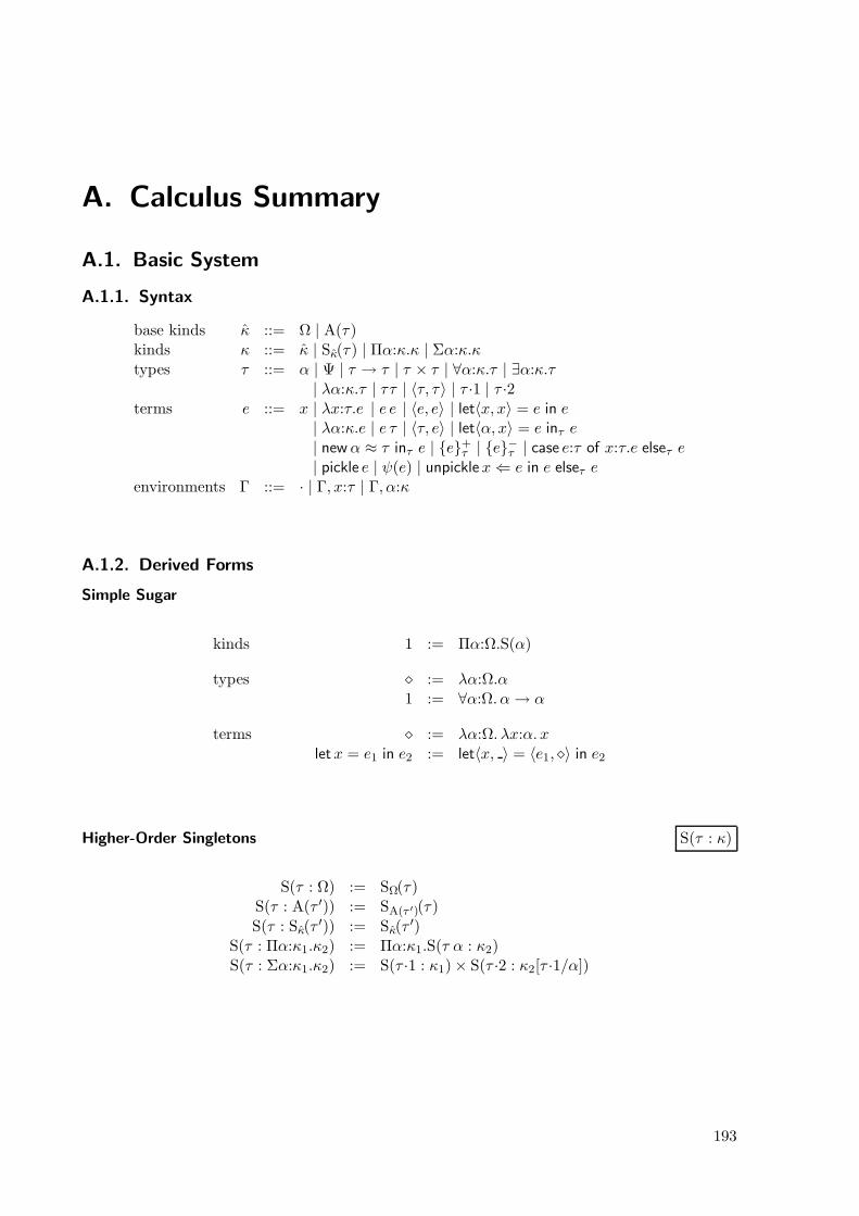
A. Calculus Summary
A.1. Basic System
A.1.1. Syntax
base kinds κ ::= Ω | A(τ)kinds κ ::= κ | Sκ(τ) | Πα:κ.κ | Σα:κ.κtypes τ ::= α | Ψ | τ → τ | τ × τ | ∀α:κ.τ | ∃α:κ.τ
| λα:κ.τ | ττ | 〈τ, τ〉 | τ ·1 | τ ·2terms e ::= x | λx:τ.e | e e | 〈e, e〉 | let〈x, x〉 = e in e
| λα:κ.e | e τ | 〈τ, e〉 | let〈α, x〉 = e inτ e| newα ≈ τ inτ e | e
+τ | e−τ | case e:τ of x:τ.e elseτ e
| pickle e | ψ(e) | unpicklex⇐ e in e elseτ eenvironments Γ ::= · | Γ, x:τ | Γ, α:κ
A.1.2. Derived Forms
Simple Sugar
kinds 1 := Πα:Ω.S(α)
types ⋄ := λα:Ω.α1 := ∀α:Ω. α→ α
terms ⋄ := λα:Ω. λx:α. xletx = e1 in e2 := let〈x, 〉 = 〈e1, ⋄〉 in e2
Higher-Order Singletons S(τ : κ)
S(τ : Ω) := SΩ(τ)S(τ : A(τ ′)) := SA(τ ′)(τ)
S(τ : Sκ(τ′)) := Sκ(τ
′)S(τ : Πα:κ1.κ2) := Πα:κ1.S(τ α : κ2)S(τ : Σα:κ1.κ2) := S(τ ·1 : κ1) × S(τ ·2 : κ2[τ ·1/α])
193
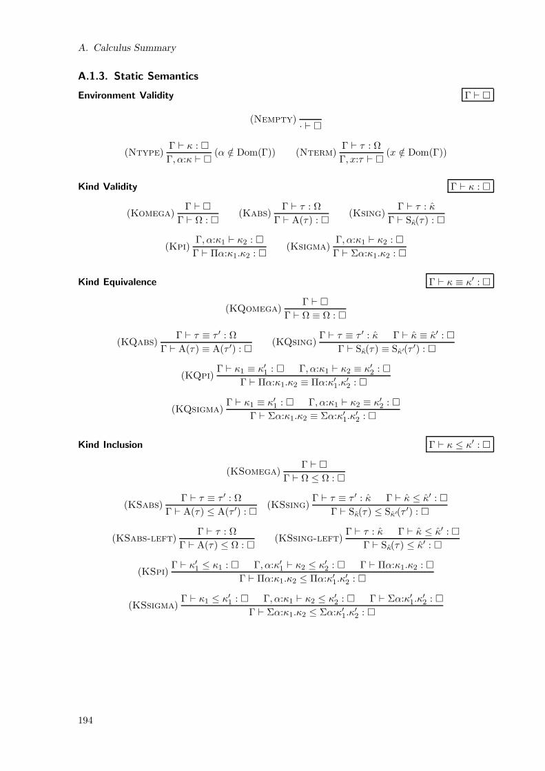
A. Calculus Summary
A.1.3. Static Semantics
Environment Validity Γ ⊢
(Nempty)· ⊢
(Ntype)Γ ⊢ κ :
Γ, α:κ ⊢ (α /∈ Dom(Γ)) (Nterm)
Γ ⊢ τ : Ω
Γ, x:τ ⊢ (x /∈ Dom(Γ))
Kind Validity Γ ⊢ κ :
(Komega)Γ ⊢
Γ ⊢ Ω : (Kabs)
Γ ⊢ τ : Ω
Γ ⊢ A(τ) : (Ksing)
Γ ⊢ τ : κ
Γ ⊢ Sκ(τ) :
(Kpi)Γ, α:κ1 ⊢ κ2 :
Γ ⊢ Πα:κ1.κ2 : (Ksigma)
Γ, α:κ1 ⊢ κ2 :
Γ ⊢ Σα:κ1.κ2 :
Kind Equivalence Γ ⊢ κ ≡ κ′ :
(KQomega)Γ ⊢
Γ ⊢ Ω ≡ Ω :
(KQabs)Γ ⊢ τ ≡ τ ′ : Ω
Γ ⊢ A(τ) ≡ A(τ ′) : (KQsing)
Γ ⊢ τ ≡ τ ′ : κ Γ ⊢ κ ≡ κ′ :
Γ ⊢ Sκ(τ) ≡ Sκ′(τ ′) :
(KQpi)Γ ⊢ κ1 ≡ κ′1 : Γ, α:κ1 ⊢ κ2 ≡ κ′2 :
Γ ⊢ Πα:κ1.κ2 ≡ Πα:κ′1.κ′2 :
(KQsigma)Γ ⊢ κ1 ≡ κ′1 : Γ, α:κ1 ⊢ κ2 ≡ κ′2 :
Γ ⊢ Σα:κ1.κ2 ≡ Σα:κ′1.κ′2 :
Kind Inclusion Γ ⊢ κ ≤ κ′ :
(KSomega)Γ ⊢
Γ ⊢ Ω ≤ Ω :
(KSabs)Γ ⊢ τ ≡ τ ′ : Ω
Γ ⊢ A(τ) ≤ A(τ ′) : (KSsing)
Γ ⊢ τ ≡ τ ′ : κ Γ ⊢ κ ≤ κ′ :
Γ ⊢ Sκ(τ) ≤ Sκ′(τ ′) :
(KSabs-left)Γ ⊢ τ : Ω
Γ ⊢ A(τ) ≤ Ω : (KSsing-left)
Γ ⊢ τ : κ Γ ⊢ κ ≤ κ′ :
Γ ⊢ Sκ(τ) ≤ κ′ :
(KSpi)Γ ⊢ κ′1 ≤ κ1 : Γ, α:κ′1 ⊢ κ2 ≤ κ′2 : Γ ⊢ Πα:κ1.κ2 :
Γ ⊢ Πα:κ1.κ2 ≤ Πα:κ′1.κ′2 :
(KSsigma)Γ ⊢ κ1 ≤ κ′1 : Γ, α:κ1 ⊢ κ2 ≤ κ′2 : Γ ⊢ Σα:κ′1.κ
′2 :
Γ ⊢ Σα:κ1.κ2 ≤ Σα:κ′1.κ′2 :
194
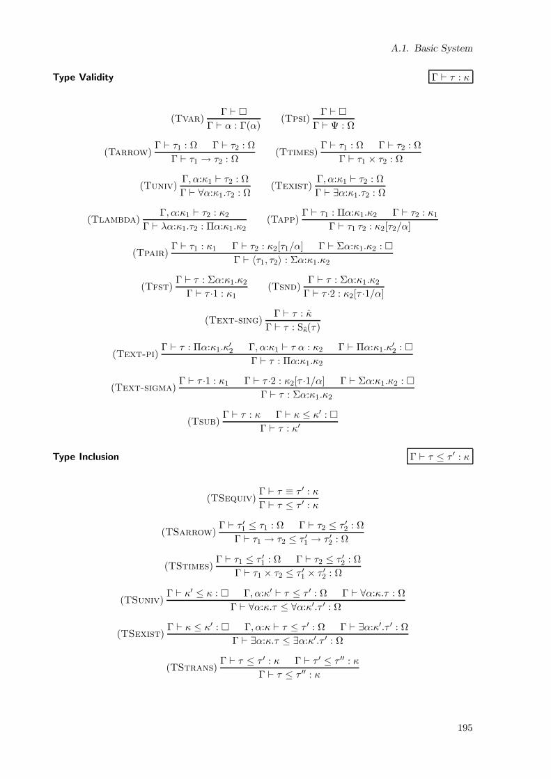
A.1. Basic System
Type Validity Γ ⊢ τ : κ
(Tvar)Γ ⊢
Γ ⊢ α : Γ(α)(Tpsi)
Γ ⊢
Γ ⊢ Ψ : Ω
(Tarrow)Γ ⊢ τ1 : Ω Γ ⊢ τ2 : Ω
Γ ⊢ τ1 → τ2 : Ω(Ttimes)
Γ ⊢ τ1 : Ω Γ ⊢ τ2 : Ω
Γ ⊢ τ1 × τ2 : Ω
(Tuniv)Γ, α:κ1 ⊢ τ2 : Ω
Γ ⊢ ∀α:κ1.τ2 : Ω(Texist)
Γ, α:κ1 ⊢ τ2 : Ω
Γ ⊢ ∃α:κ1.τ2 : Ω
(Tlambda)Γ, α:κ1 ⊢ τ2 : κ2
Γ ⊢ λα:κ1.τ2 : Πα:κ1.κ2(Tapp)
Γ ⊢ τ1 : Πα:κ1.κ2 Γ ⊢ τ2 : κ1
Γ ⊢ τ1 τ2 : κ2[τ2/α]
(Tpair)Γ ⊢ τ1 : κ1 Γ ⊢ τ2 : κ2[τ1/α] Γ ⊢ Σα:κ1.κ2 :
Γ ⊢ 〈τ1, τ2〉 : Σα:κ1.κ2
(Tfst)Γ ⊢ τ : Σα:κ1.κ2
Γ ⊢ τ ·1 : κ1(Tsnd)
Γ ⊢ τ : Σα:κ1.κ2
Γ ⊢ τ ·2 : κ2[τ ·1/α]
(Text-sing)Γ ⊢ τ : κ
Γ ⊢ τ : Sκ(τ)
(Text-pi)Γ ⊢ τ : Πα:κ1.κ
′2 Γ, α:κ1 ⊢ τ α : κ2 Γ ⊢ Πα:κ1.κ
′2 :
Γ ⊢ τ : Πα:κ1.κ2
(Text-sigma)Γ ⊢ τ ·1 : κ1 Γ ⊢ τ ·2 : κ2[τ ·1/α] Γ ⊢ Σα:κ1.κ2 :
Γ ⊢ τ : Σα:κ1.κ2
(Tsub)Γ ⊢ τ : κ Γ ⊢ κ ≤ κ′ :
Γ ⊢ τ : κ′
Type Inclusion Γ ⊢ τ ≤ τ ′ : κ
(TSequiv)Γ ⊢ τ ≡ τ ′ : κ
Γ ⊢ τ ≤ τ ′ : κ
(TSarrow)Γ ⊢ τ ′1 ≤ τ1 : Ω Γ ⊢ τ2 ≤ τ ′2 : Ω
Γ ⊢ τ1 → τ2 ≤ τ ′1 → τ ′2 : Ω
(TStimes)Γ ⊢ τ1 ≤ τ ′1 : Ω Γ ⊢ τ2 ≤ τ ′2 : Ω
Γ ⊢ τ1 × τ2 ≤ τ ′1 × τ ′2 : Ω
(TSuniv)Γ ⊢ κ′ ≤ κ : Γ, α:κ′ ⊢ τ ≤ τ ′ : Ω Γ ⊢ ∀α:κ.τ : Ω
Γ ⊢ ∀α:κ.τ ≤ ∀α:κ′.τ ′ : Ω
(TSexist)Γ ⊢ κ ≤ κ′ : Γ, α:κ ⊢ τ ≤ τ ′ : Ω Γ ⊢ ∃α:κ′.τ ′ : Ω
Γ ⊢ ∃α:κ.τ ≤ ∃α:κ′.τ ′ : Ω
(TStrans)Γ ⊢ τ ≤ τ ′ : κ Γ ⊢ τ ′ ≤ τ ′′ : κ
Γ ⊢ τ ≤ τ ′′ : κ
195
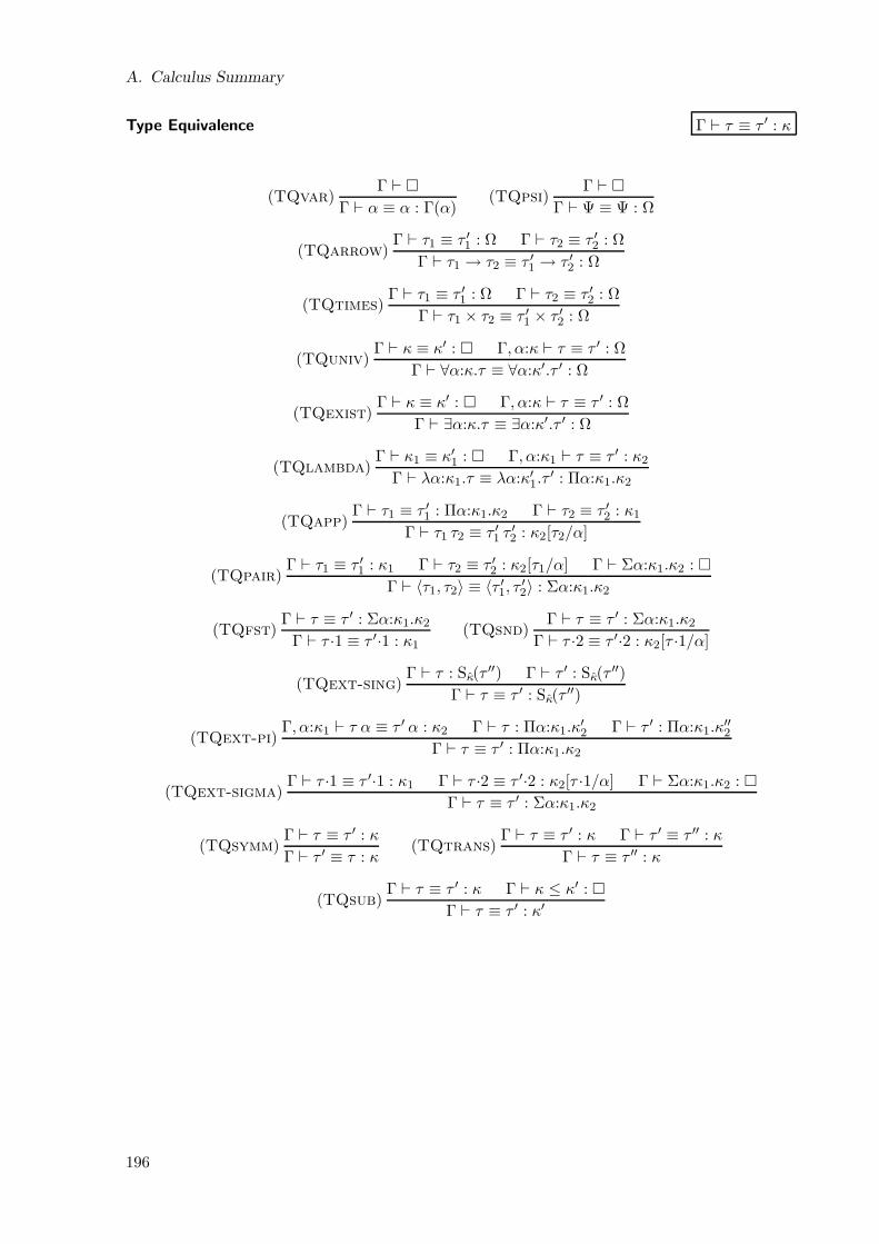
A. Calculus Summary
Type Equivalence Γ ⊢ τ ≡ τ ′ : κ
(TQvar)Γ ⊢
Γ ⊢ α ≡ α : Γ(α)(TQpsi)
Γ ⊢
Γ ⊢ Ψ ≡ Ψ : Ω
(TQarrow)Γ ⊢ τ1 ≡ τ ′1 : Ω Γ ⊢ τ2 ≡ τ ′2 : Ω
Γ ⊢ τ1 → τ2 ≡ τ ′1 → τ ′2 : Ω
(TQtimes)Γ ⊢ τ1 ≡ τ ′1 : Ω Γ ⊢ τ2 ≡ τ ′2 : Ω
Γ ⊢ τ1 × τ2 ≡ τ ′1 × τ ′2 : Ω
(TQuniv)Γ ⊢ κ ≡ κ′ : Γ, α:κ ⊢ τ ≡ τ ′ : Ω
Γ ⊢ ∀α:κ.τ ≡ ∀α:κ′.τ ′ : Ω
(TQexist)Γ ⊢ κ ≡ κ′ : Γ, α:κ ⊢ τ ≡ τ ′ : Ω
Γ ⊢ ∃α:κ.τ ≡ ∃α:κ′.τ ′ : Ω
(TQlambda)Γ ⊢ κ1 ≡ κ′1 : Γ, α:κ1 ⊢ τ ≡ τ ′ : κ2
Γ ⊢ λα:κ1.τ ≡ λα:κ′1.τ′ : Πα:κ1.κ2
(TQapp)Γ ⊢ τ1 ≡ τ ′1 : Πα:κ1.κ2 Γ ⊢ τ2 ≡ τ ′2 : κ1
Γ ⊢ τ1 τ2 ≡ τ ′1 τ′2 : κ2[τ2/α]
(TQpair)Γ ⊢ τ1 ≡ τ ′1 : κ1 Γ ⊢ τ2 ≡ τ ′2 : κ2[τ1/α] Γ ⊢ Σα:κ1.κ2 :
Γ ⊢ 〈τ1, τ2〉 ≡ 〈τ ′1, τ′2〉 : Σα:κ1.κ2
(TQfst)Γ ⊢ τ ≡ τ ′ : Σα:κ1.κ2
Γ ⊢ τ ·1 ≡ τ ′·1 : κ1(TQsnd)
Γ ⊢ τ ≡ τ ′ : Σα:κ1.κ2
Γ ⊢ τ ·2 ≡ τ ′·2 : κ2[τ ·1/α]
(TQext-sing)Γ ⊢ τ : Sκ(τ
′′) Γ ⊢ τ ′ : Sκ(τ′′)
Γ ⊢ τ ≡ τ ′ : Sκ(τ′′)
(TQext-pi)Γ, α:κ1 ⊢ τ α ≡ τ ′ α : κ2 Γ ⊢ τ : Πα:κ1.κ
′2 Γ ⊢ τ ′ : Πα:κ1.κ
′′2
Γ ⊢ τ ≡ τ ′ : Πα:κ1.κ2
(TQext-sigma)Γ ⊢ τ ·1 ≡ τ ′·1 : κ1 Γ ⊢ τ ·2 ≡ τ ′·2 : κ2[τ ·1/α] Γ ⊢ Σα:κ1.κ2 :
Γ ⊢ τ ≡ τ ′ : Σα:κ1.κ2
(TQsymm)Γ ⊢ τ ≡ τ ′ : κ
Γ ⊢ τ ′ ≡ τ : κ(TQtrans)
Γ ⊢ τ ≡ τ ′ : κ Γ ⊢ τ ′ ≡ τ ′′ : κ
Γ ⊢ τ ≡ τ ′′ : κ
(TQsub)Γ ⊢ τ ≡ τ ′ : κ Γ ⊢ κ ≤ κ′ :
Γ ⊢ τ ≡ τ ′ : κ′
196
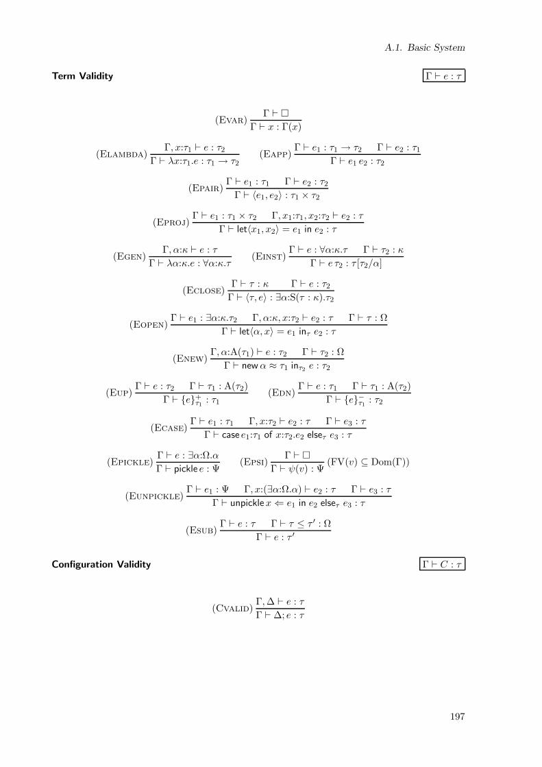
A.1. Basic System
Term Validity Γ ⊢ e : τ
(Evar)Γ ⊢
Γ ⊢ x : Γ(x)
(Elambda)Γ, x:τ1 ⊢ e : τ2
Γ ⊢ λx:τ1.e : τ1 → τ2(Eapp)
Γ ⊢ e1 : τ1 → τ2 Γ ⊢ e2 : τ1Γ ⊢ e1 e2 : τ2
(Epair)Γ ⊢ e1 : τ1 Γ ⊢ e2 : τ2
Γ ⊢ 〈e1, e2〉 : τ1 × τ2
(Eproj)Γ ⊢ e1 : τ1 × τ2 Γ, x1:τ1, x2:τ2 ⊢ e2 : τ
Γ ⊢ let〈x1, x2〉 = e1 in e2 : τ
(Egen)Γ, α:κ ⊢ e : τ
Γ ⊢ λα:κ.e : ∀α:κ.τ(Einst)
Γ ⊢ e : ∀α:κ.τ Γ ⊢ τ2 : κ
Γ ⊢ e τ2 : τ [τ2/α]
(Eclose)Γ ⊢ τ : κ Γ ⊢ e : τ2
Γ ⊢ 〈τ, e〉 : ∃α:S(τ : κ).τ2
(Eopen)Γ ⊢ e1 : ∃α:κ.τ2 Γ, α:κ, x:τ2 ⊢ e2 : τ Γ ⊢ τ : Ω
Γ ⊢ let〈α, x〉 = e1 inτ e2 : τ
(Enew)Γ, α:A(τ1) ⊢ e : τ2 Γ ⊢ τ2 : Ω
Γ ⊢ newα ≈ τ1 inτ2 e : τ2
(Eup)Γ ⊢ e : τ2 Γ ⊢ τ1 : A(τ2)
Γ ⊢ e+τ1 : τ1
(Edn)Γ ⊢ e : τ1 Γ ⊢ τ1 : A(τ2)
Γ ⊢ e−τ1 : τ2
(Ecase)Γ ⊢ e1 : τ1 Γ, x:τ2 ⊢ e2 : τ Γ ⊢ e3 : τ
Γ ⊢ case e1:τ1 of x:τ2.e2 elseτ e3 : τ
(Epickle)Γ ⊢ e : ∃α:Ω.α
Γ ⊢ pickle e : Ψ(Epsi)
Γ ⊢
Γ ⊢ ψ(v) : Ψ(FV(v) ⊆ Dom(Γ))
(Eunpickle)Γ ⊢ e1 : Ψ Γ, x:(∃α:Ω.α) ⊢ e2 : τ Γ ⊢ e3 : τ
Γ ⊢ unpicklex⇐ e1 in e2 elseτ e3 : τ
(Esub)Γ ⊢ e : τ Γ ⊢ τ ≤ τ ′ : Ω
Γ ⊢ e : τ ′
Configuration Validity Γ ⊢ C : τ
(Cvalid)Γ,∆ ⊢ e : τ
Γ ⊢ ∆; e : τ
197
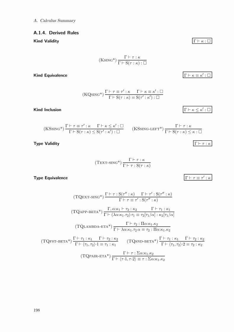
A. Calculus Summary
A.1.4. Derived Rules
Kind Validity Γ ⊢ κ :
(Ksing*)Γ ⊢ τ : κ
Γ ⊢ S(τ : κ) :
Kind Equivalence Γ ⊢ κ ≡ κ′ :
(KQsing*)Γ ⊢ τ ≡ τ ′ : κ Γ ⊢ κ ≡ κ′ :
Γ ⊢ S(τ : κ) ≡ S(τ ′ : κ′) :
Kind Inclusion Γ ⊢ κ ≤ κ′ :
(KSsing*)Γ ⊢ τ ≡ τ ′ : κ Γ ⊢ κ ≤ κ′ :
Γ ⊢ S(τ : κ) ≤ S(τ ′ : κ′) : (KSsing-left*)
Γ ⊢ τ : κ
Γ ⊢ S(τ : κ) ≤ κ :
Type Validity Γ ⊢ τ : κ
(Text-sing*)Γ ⊢ τ : κ
Γ ⊢ τ : S(τ : κ)
Type Equivalence Γ ⊢ τ ≡ τ ′ : κ
(TQext-sing*)Γ ⊢ τ : S(τ ′′ : κ) Γ ⊢ τ ′ : S(τ ′′ : κ)
Γ ⊢ τ ≡ τ ′ : S(τ ′′ : κ)
(TQapp-beta*)Γ, α:κ1 ⊢ τ2 : κ2 Γ ⊢ τ1 : κ1
Γ ⊢ (λα:κ1.τ2) τ1 ≡ τ2[τ1/α] : κ2[τ1/α]
(TQlambda-eta*)Γ ⊢ τ2 : Πα:κ1.κ2
Γ ⊢ λα:κ1.τ2 α ≡ τ2 : Πα:κ1.κ2
(TQfst-beta*)Γ ⊢ τ1 : κ1 Γ ⊢ τ2 : κ2
Γ ⊢ 〈τ1, τ2〉·1 ≡ τ1 : κ1(TQsnd-beta*)
Γ ⊢ τ1 : κ1 Γ ⊢ τ2 : κ2
Γ ⊢ 〈τ1, τ2〉·2 ≡ τ2 : κ2
(TQpair-eta*)Γ ⊢ τ : Σα:κ1.κ2
Γ ⊢ 〈τ ·1, τ ·2〉 ≡ τ : Σα:κ1.κ2
198
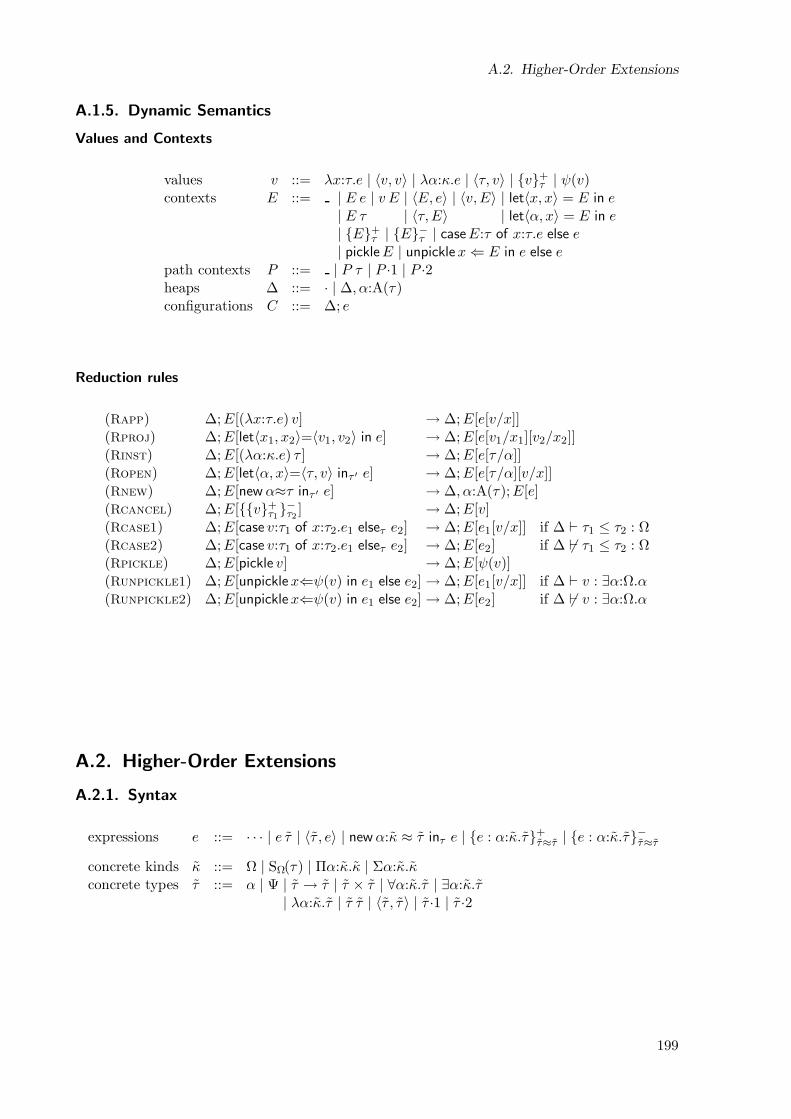
A.2. Higher-Order Extensions
A.1.5. Dynamic Semantics
Values and Contexts
values v ::= λx:τ.e | 〈v, v〉 | λα:κ.e | 〈τ, v〉 | v+τ | ψ(v)
contexts E ::= | E e | v E | 〈E, e〉 | 〈v,E〉 | let〈x, x〉 = E in e| E τ | 〈τ,E〉 | let〈α, x〉 = E in e| E+
τ | E−τ | caseE:τ of x:τ.e else e| pickleE | unpicklex⇐ E in e else e
path contexts P ::= | P τ | P ·1 | P ·2heaps ∆ ::= · | ∆, α:A(τ)configurations C ::= ∆; e
Reduction rules
(Rapp) ∆;E[(λx:τ.e) v] → ∆;E[e[v/x]](Rproj) ∆;E[let〈x1, x2〉=〈v1, v2〉 in e] → ∆;E[e[v1/x1][v2/x2]](Rinst) ∆;E[(λα:κ.e) τ ] → ∆;E[e[τ/α]](Ropen) ∆;E[let〈α, x〉=〈τ, v〉 inτ ′ e] → ∆;E[e[τ/α][v/x]](Rnew) ∆;E[new α≈τ inτ ′ e] → ∆, α:A(τ);E[e](Rcancel) ∆;E[v+
τ1−τ2 ] → ∆;E[v]
(Rcase1) ∆;E[case v:τ1 of x:τ2.e1 elseτ e2] → ∆;E[e1[v/x]] if ∆ ⊢ τ1 ≤ τ2 : Ω(Rcase2) ∆;E[case v:τ1 of x:τ2.e1 elseτ e2] → ∆;E[e2] if ∆ 6⊢ τ1 ≤ τ2 : Ω(Rpickle) ∆;E[pickle v] → ∆;E[ψ(v)](Runpickle1) ∆;E[unpicklex⇐ψ(v) in e1 else e2] → ∆;E[e1[v/x]] if ∆ ⊢ v : ∃α:Ω.α(Runpickle2) ∆;E[unpicklex⇐ψ(v) in e1 else e2] → ∆;E[e2] if ∆ 6⊢ v : ∃α:Ω.α
A.2. Higher-Order Extensions
A.2.1. Syntax
expressions e ::= · · · | e τ | 〈τ , e〉 | newα:κ ≈ τ inτ e | e : α:κ.τ+τ≈τ | e : α:κ.τ−τ≈τ
concrete kinds κ ::= Ω | SΩ(τ) | Πα:κ.κ | Σα:κ.κconcrete types τ ::= α | Ψ | τ → τ | τ × τ | ∀α:κ.τ | ∃α:κ.τ
| λα:κ.τ | τ τ | 〈τ , τ 〉 | τ ·1 | τ ·2
199
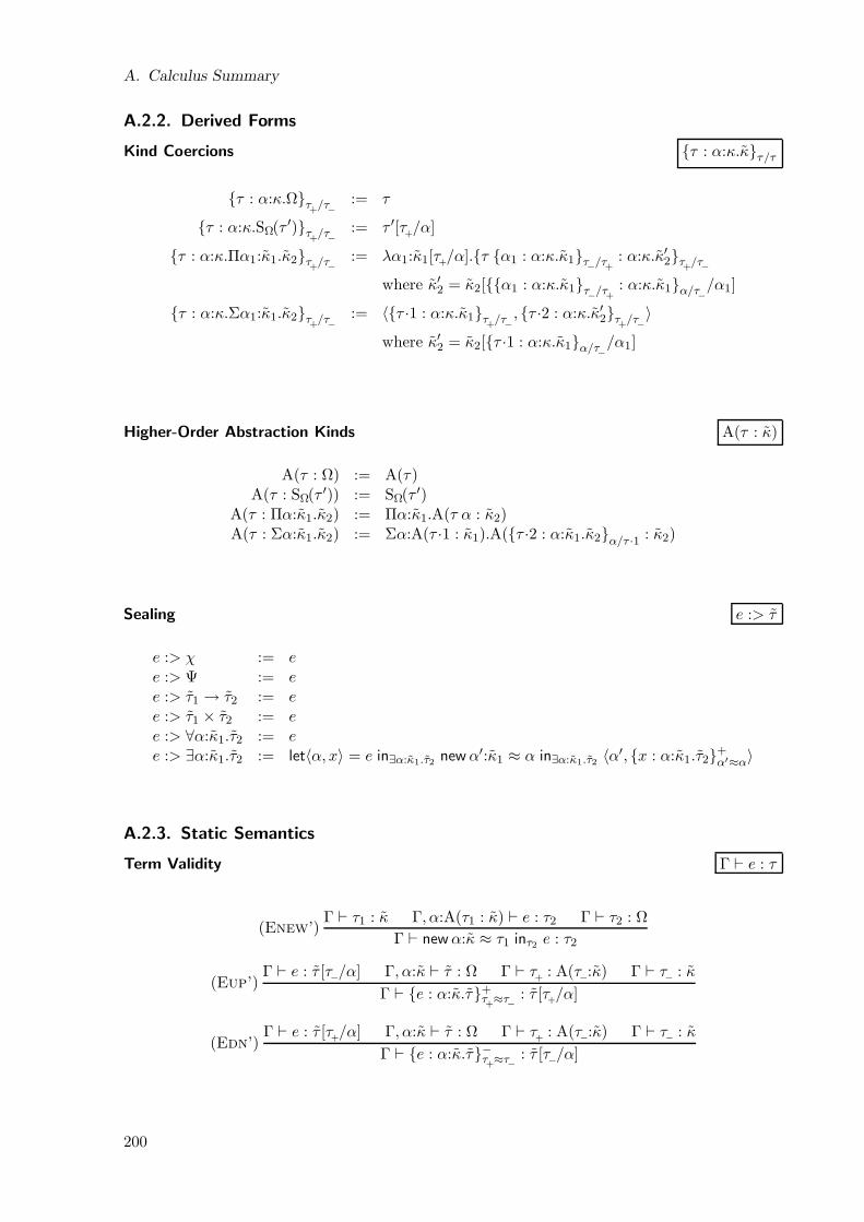
A. Calculus Summary
A.2.2. Derived Forms
Kind Coercions τ : α:κ.κτ/τ
τ : α:κ.Ωτ+
/τ−:= τ
τ : α:κ.SΩ(τ ′)τ+
/τ−:= τ ′[τ
+/α]
τ : α:κ.Πα1:κ1.κ2τ+
/τ−:= λα1:κ1[τ+/α].τ α1 : α:κ.κ1τ−/τ
+: α:κ.κ′2τ
+/τ−
where κ′2 = κ2[α1 : α:κ.κ1τ−/τ+
: α:κ.κ1α/τ−/α1]
τ : α:κ.Σα1:κ1.κ2τ+
/τ−:= 〈τ ·1 : α:κ.κ1τ
+/τ−, τ ·2 : α:κ.κ′2τ
+/τ−
〉
where κ′2 = κ2[τ ·1 : α:κ.κ1α/τ−/α1]
Higher-Order Abstraction Kinds A(τ : κ)
A(τ : Ω) := A(τ)A(τ : SΩ(τ ′)) := SΩ(τ ′)
A(τ : Πα:κ1.κ2) := Πα:κ1.A(τ α : κ2)A(τ : Σα:κ1.κ2) := Σα:A(τ ·1 : κ1).A(τ ·2 : α:κ1.κ2α/τ ·1 : κ2)
Sealing e :> τ
e :> χ := ee :> Ψ := ee :> τ1 → τ2 := ee :> τ1 × τ2 := ee :> ∀α:κ1.τ2 := ee :> ∃α:κ1.τ2 := let〈α, x〉 = e in∃α:κ1.τ2 newα′:κ1 ≈ α in∃α:κ1.τ2 〈α′, x : α:κ1.τ2
+α′≈α〉
A.2.3. Static Semantics
Term Validity Γ ⊢ e : τ
(Enew’)Γ ⊢ τ1 : κ Γ, α:A(τ1 : κ) ⊢ e : τ2 Γ ⊢ τ2 : Ω
Γ ⊢ newα:κ ≈ τ1 inτ2 e : τ2
(Eup’)Γ ⊢ e : τ [τ−/α] Γ, α:κ ⊢ τ : Ω Γ ⊢ τ
+: A(τ−:κ) Γ ⊢ τ− : κ
Γ ⊢ e : α:κ.τ+τ+≈τ−
: τ [τ+/α]
(Edn’)Γ ⊢ e : τ [τ
+/α] Γ, α:κ ⊢ τ : Ω Γ ⊢ τ
+: A(τ−:κ) Γ ⊢ τ− : κ
Γ ⊢ e : α:κ.τ−τ+≈τ−
: τ [τ−/α]
200
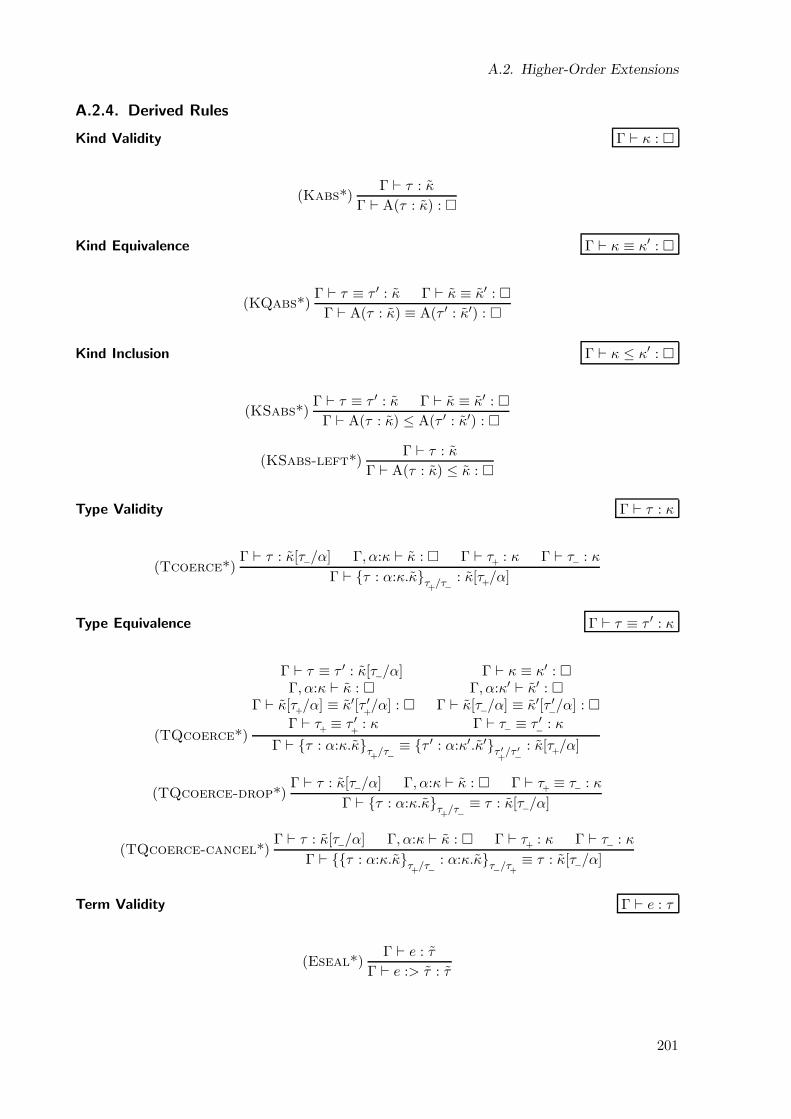
A.2. Higher-Order Extensions
A.2.4. Derived Rules
Kind Validity Γ ⊢ κ :
(Kabs*)Γ ⊢ τ : κ
Γ ⊢ A(τ : κ) :
Kind Equivalence Γ ⊢ κ ≡ κ′ :
(KQabs*)Γ ⊢ τ ≡ τ ′ : κ Γ ⊢ κ ≡ κ′ :
Γ ⊢ A(τ : κ) ≡ A(τ ′ : κ′) :
Kind Inclusion Γ ⊢ κ ≤ κ′ :
(KSabs*)Γ ⊢ τ ≡ τ ′ : κ Γ ⊢ κ ≡ κ′ :
Γ ⊢ A(τ : κ) ≤ A(τ ′ : κ′) :
(KSabs-left*)Γ ⊢ τ : κ
Γ ⊢ A(τ : κ) ≤ κ :
Type Validity Γ ⊢ τ : κ
(Tcoerce*)Γ ⊢ τ : κ[τ−/α] Γ, α:κ ⊢ κ : Γ ⊢ τ
+: κ Γ ⊢ τ− : κ
Γ ⊢ τ : α:κ.κτ+
/τ−: κ[τ
+/α]
Type Equivalence Γ ⊢ τ ≡ τ ′ : κ
(TQcoerce*)
Γ ⊢ τ ≡ τ ′ : κ[τ−/α] Γ ⊢ κ ≡ κ′ : Γ, α:κ ⊢ κ : Γ, α:κ′ ⊢ κ′ :
Γ ⊢ κ[τ+/α] ≡ κ′[τ ′
+/α] : Γ ⊢ κ[τ−/α] ≡ κ′[τ ′
−/α] :
Γ ⊢ τ+≡ τ ′
+: κ Γ ⊢ τ− ≡ τ ′
−: κ
Γ ⊢ τ : α:κ.κτ+
/τ−≡ τ ′ : α:κ′.κ′τ ′
+/τ ′
−
: κ[τ+/α]
(TQcoerce-drop*)Γ ⊢ τ : κ[τ−/α] Γ, α:κ ⊢ κ : Γ ⊢ τ
+≡ τ− : κ
Γ ⊢ τ : α:κ.κτ+
/τ−≡ τ : κ[τ−/α]
(TQcoerce-cancel*)Γ ⊢ τ : κ[τ−/α] Γ, α:κ ⊢ κ : Γ ⊢ τ
+: κ Γ ⊢ τ− : κ
Γ ⊢ τ : α:κ.κτ+
/τ−: α:κ.κτ−/τ
+
≡ τ : κ[τ−/α]
Term Validity Γ ⊢ e : τ
(Eseal*)Γ ⊢ e : τ
Γ ⊢ e :> τ : τ
201
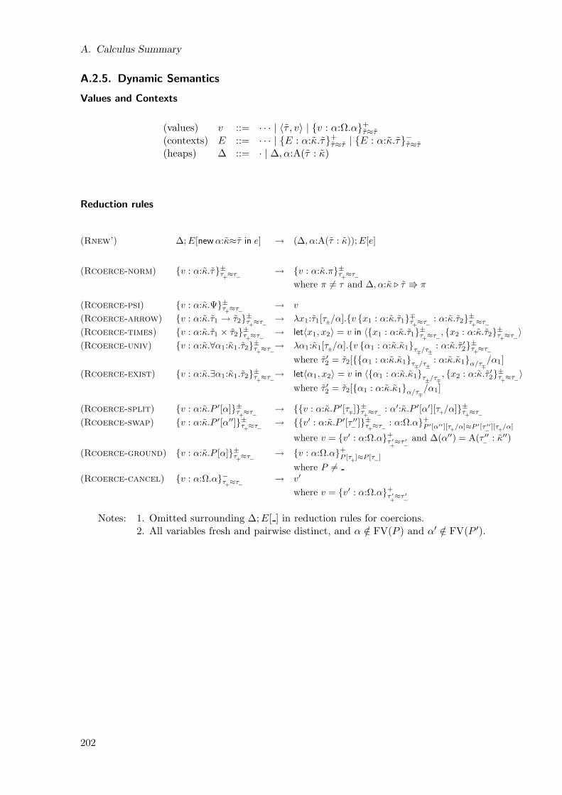
A. Calculus Summary
A.2.5. Dynamic Semantics
Values and Contexts
(values) v ::= · · · | 〈τ , v〉 | v : α:Ω.α+τ≈τ
(contexts) E ::= · · · | E : α:κ.τ+τ≈τ | E : α:κ.τ−τ≈τ
(heaps) ∆ ::= · | ∆, α:A(τ : κ)
Reduction rules
(Rnew’) ∆;E[newα:κ≈τ in e] → (∆, α:A(τ : κ));E[e]
(Rcoerce-norm) v : α:κ.τ±τ+≈τ
−→ v : α:κ.π±τ
+≈τ
−
where π 6= τ and ∆, α:κ ⊲ τ π
(Rcoerce-psi) v : α:κ.Ψ±τ+≈τ−
→ v
(Rcoerce-arrow) v : α:κ.τ1 → τ2±τ+≈τ−
→ λx1:τ1[τ±/α].v x1 : α:κ.τ1∓τ+≈τ−
: α:κ.τ2±τ+≈τ−
(Rcoerce-times) v : α:κ.τ1 × τ2±τ+≈τ−
→ let〈x1, x2〉 = v in 〈x1 : α:κ.τ1±τ+≈τ−
, x2 : α:κ.τ2±τ+≈τ−
〉
(Rcoerce-univ) v : α:κ.∀α1:κ1.τ2±τ+≈τ
−→ λα1:κ1[τ±/α].v α1 : α:κ.κ1τ∓/τ±
: α:κ.τ ′2±τ+≈τ
−
where τ ′2 = τ2[α1 : α:κ.κ1τ∓/τ±: α:κ.κ1α/τ∓
/α1]
(Rcoerce-exist) v : α:κ.∃α1:κ1.τ2±τ+≈τ−
→ let〈α1, x2〉 = v in 〈α1 : α:κ.κ1τ±/τ∓, x2 : α:κ.τ ′2
±τ+≈τ−
〉
where τ ′2 = τ2[α1 : α:κ.κ1α/τ∓/α1]
(Rcoerce-split) v : α:κ.P ′[α]±τ+≈τ
−→ v : α:κ.P ′[τ∓]±τ
+≈τ
−: α′:κ.P ′[α′][τ+/α]±τ
+≈τ
−
(Rcoerce-swap) v : α:κ.P ′[α′′]±τ+≈τ
−→ v′ : α:κ.P ′[τ ′′
−]±τ
+≈τ
−: α:Ω.α+
P ′[α′′][τ+
/α]≈P ′[τ ′′−
][τ+
/α]
where v = v′ : α:Ω.α+τ ′+≈τ ′
−and ∆(α′′) = A(τ ′′
−: κ′′)
(Rcoerce-ground) v : α:κ.P [α]±τ+≈τ
−→ v : α:Ω.α+
P [τ+]≈P [τ
−]
where P 6=(Rcoerce-cancel) v : α:Ω.α−τ
+≈τ−
→ v′
where v = v′ : α:Ω.α+τ ′+≈τ ′
−
Notes: 1. Omitted surrounding ∆;E[ ] in reduction rules for coercions.2. All variables fresh and pairwise distinct, and α /∈ FV(P ) and α′ /∈ FV(P ′).
202
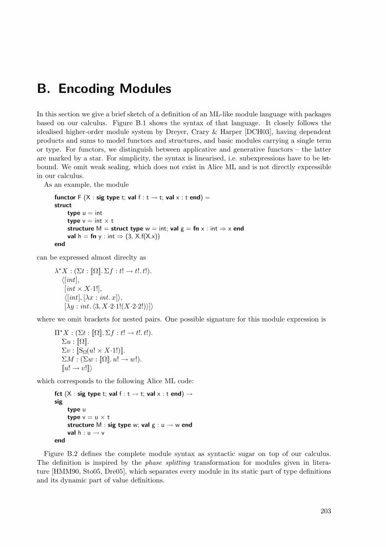
B. Encoding Modules
In this section we give a brief sketch of a definition of an ML-like module language with packagesbased on our calculus. Figure B.1 shows the syntax of that language. It closely follows theidealised higher-order module system by Dreyer, Crary & Harper [DCH03], having dependentproducts and sums to model functors and structures, and basic modules carrying a single termor type. For functors, we distinguish between applicative and generative functors – the latterare marked by a star. For simplicity, the syntax is linearised, i.e. subexpressions have to be let-bound. We omit weak sealing, which does not exist in Alice ML and is not directly expressiblein our calculus.
As an example, the module
functor F (X : sig type t; val f : t → t; val x : t end) =struct
type u = inttype v = int × tstructure M = struct type w = int; val g = fn x : int ⇒ x end
val h = fn y : int ⇒ (3, X.f(X.x))end
can be expressed almost direclty as
λ∗X : (Σt : [[Ω]].Σf : t! → t!. t!).〈[int ],[int ×X·1!],〈[int ], [λx : int . x]〉,[λy : int . 〈3,X·2·1!(X·2·2!)〉]〉
where we omit brackets for nested pairs. One possible signature for this module expression is
Π∗X : (Σt : [[Ω]].Σf : t! → t!. t!).Σu : [[Ω]].Σv : [[SΩ(u! ×X·1!)]].ΣM : (Σw : [[Ω]]. u! → w!).[[u! → v!]]〉
which corresponds to the following Alice ML code:
fct (X : sig type t; val f : t → t; val x : t end) →sig
type utype v = u × tstructure M : sig type w; val g : u → w end
val h : u → vend
Figure B.2 defines the complete module syntax as syntactic sugar on top of our calculus.The definition is inspired by the phase splitting transformation for modules given in litera-ture [HMM90, Sto05, Dre05], which separates every module in its static part of type definitionsand its dynamic part of value definitions.
203
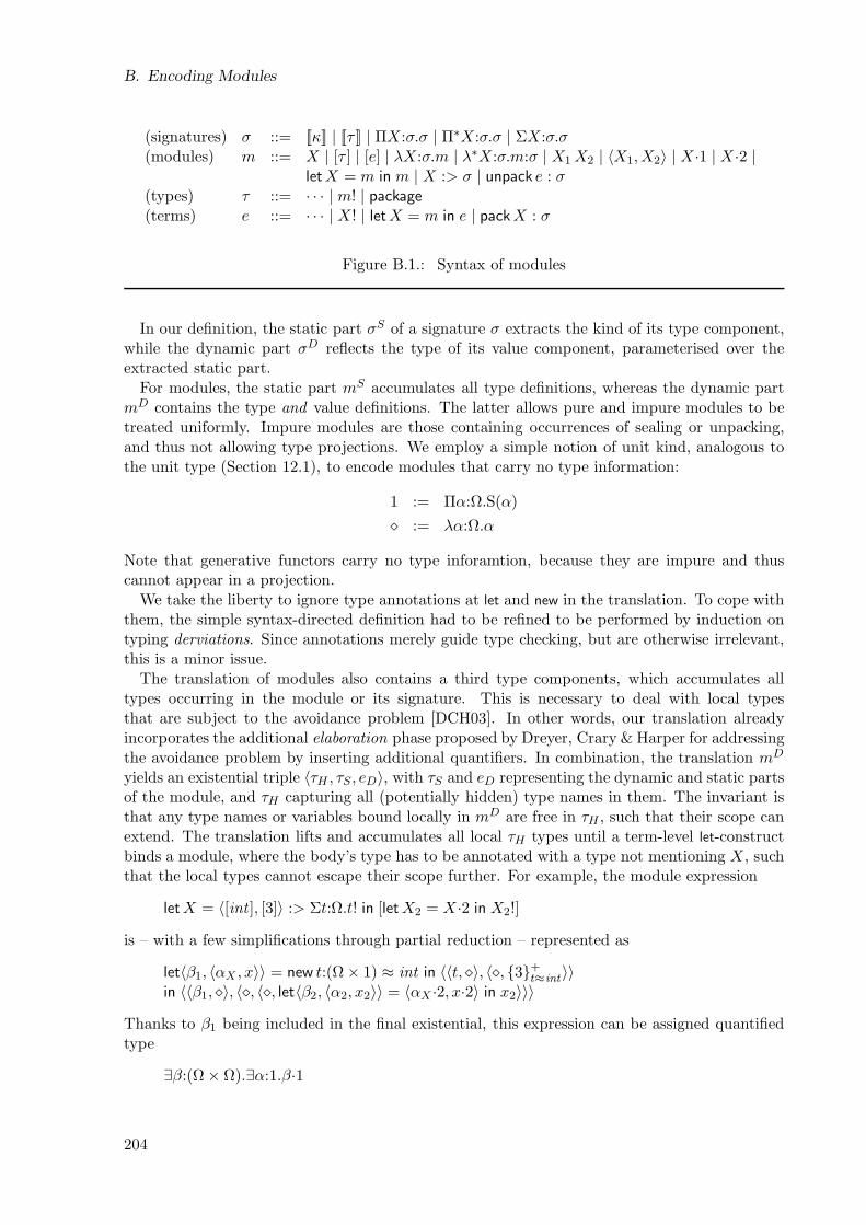
B. Encoding Modules
(signatures) σ ::= [[κ]] | [[τ ]] | ΠX:σ.σ | Π∗X:σ.σ | ΣX:σ.σ(modules) m ::= X | [τ ] | [e] | λX:σ.m | λ∗X:σ.m:σ | X1X2 | 〈X1,X2〉 | X·1 | X·2 |
letX = m in m | X :> σ | unpack e : σ(types) τ ::= · · · | m! | package(terms) e ::= · · · | X! | letX = m in e | packX : σ
Figure B.1.: Syntax of modules
In our definition, the static part σS of a signature σ extracts the kind of its type component,while the dynamic part σD reflects the type of its value component, parameterised over theextracted static part.
For modules, the static part mS accumulates all type definitions, whereas the dynamic partmD contains the type and value definitions. The latter allows pure and impure modules to betreated uniformly. Impure modules are those containing occurrences of sealing or unpacking,and thus not allowing type projections. We employ a simple notion of unit kind, analogous tothe unit type (Section 12.1), to encode modules that carry no type information:
1 := Πα:Ω.S(α)
⋄ := λα:Ω.α
Note that generative functors carry no type inforamtion, because they are impure and thuscannot appear in a projection.
We take the liberty to ignore type annotations at let and new in the translation. To cope withthem, the simple syntax-directed definition had to be refined to be performed by induction ontyping derviations. Since annotations merely guide type checking, but are otherwise irrelevant,this is a minor issue.
The translation of modules also contains a third type components, which accumulates alltypes occurring in the module or its signature. This is necessary to deal with local typesthat are subject to the avoidance problem [DCH03]. In other words, our translation alreadyincorporates the additional elaboration phase proposed by Dreyer, Crary & Harper for addressingthe avoidance problem by inserting additional quantifiers. In combination, the translation mD
yields an existential triple 〈τH , τS, eD〉, with τS and eD representing the dynamic and static partsof the module, and τH capturing all (potentially hidden) type names in them. The invariant isthat any type names or variables bound locally in mD are free in τH , such that their scope canextend. The translation lifts and accumulates all local τH types until a term-level let-constructbinds a module, where the body’s type has to be annotated with a type not mentioning X, suchthat the local types cannot escape their scope further. For example, the module expression
letX = 〈[int ], [3]〉 :> Σt:Ω.t! in [letX2 = X·2 in X2!]
is – with a few simplifications through partial reduction – represented as
let〈β1, 〈αX , x〉〉 = new t:(Ω × 1) ≈ int in 〈〈t, ⋄〉, 〈⋄, 3+t≈int
〉〉in 〈〈β1, ⋄〉, 〈⋄, 〈⋄, let〈β2, 〈α2, x2〉〉 = 〈αX ·2, x·2〉 in x2〉〉〉
Thanks to β1 being included in the final existential, this expression can be assigned quantifiedtype
∃β:(Ω × Ω).∃α:1.β·1
204
Without the outer quantifier no closed type could be assigned.The novel aspects of the translation are with respect to the sealing operator, which dynamically
generates fresh type names as investigated in Section 13.5, and the addition of packages, whichfollows the definitions of packages given in Section 12.3.2. Note however how the pack constructrefines the package signature such that its static part becomes transparent with singleton kind.This implements the behaviour discussed in Section 4.4.1.
We conjecture that the translation is correct relative to a module type system as the one givenby Dreyer, Crary & Harper and extended with packages by ourselves [Ros06], but leave a prooffor future work.
205
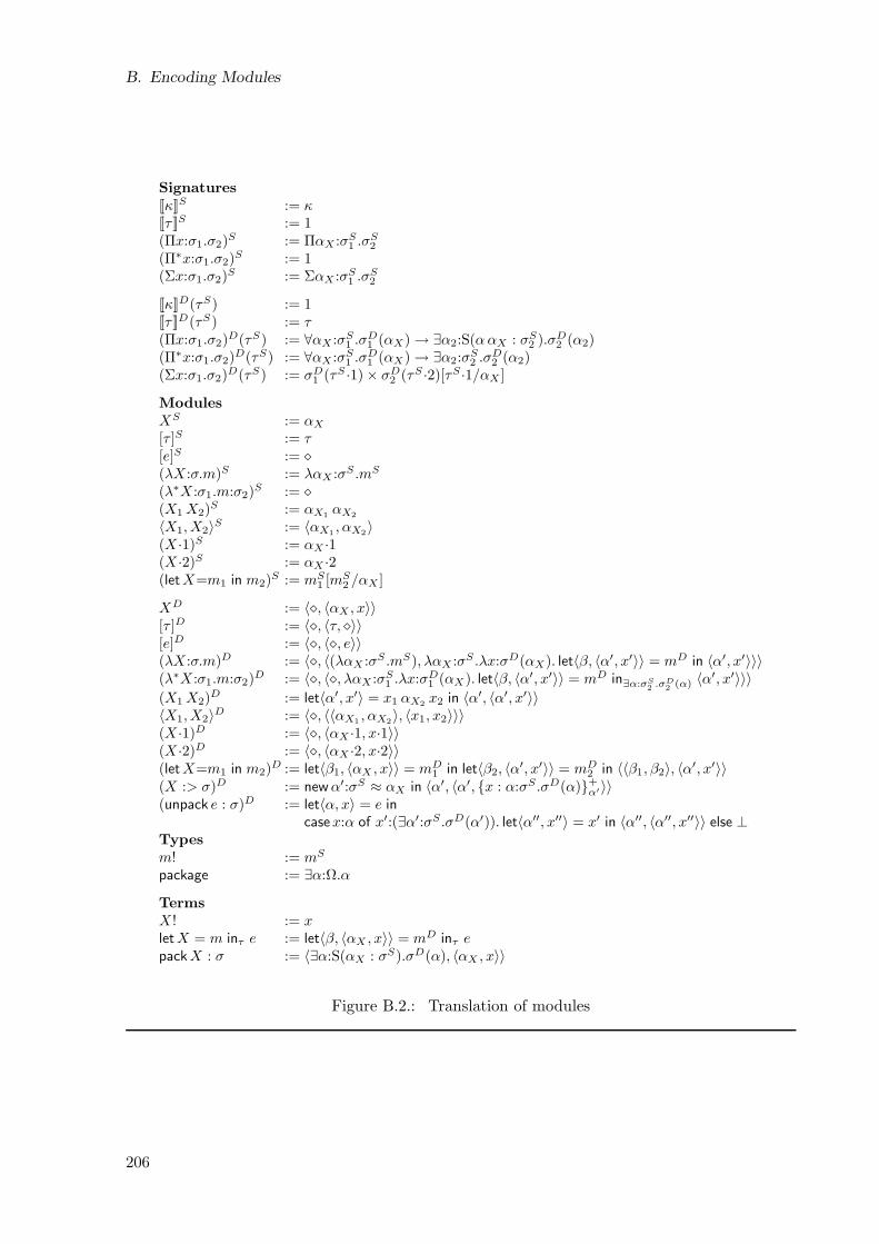
B. Encoding Modules
Signatures
[[κ]]S := κ[[τ ]]S := 1(Πx:σ1.σ2)
S := ΠαX :σS1 .σ
S2
(Π∗x:σ1.σ2)S := 1
(Σx:σ1.σ2)S := ΣαX :σS
1 .σS2
[[κ]]D(τS) := 1[[τ ]]D(τS) := τ(Πx:σ1.σ2)
D(τS) := ∀αX :σS1 .σ
D1 (αX) → ∃α2:S(ααX : σS
2 ).σD2 (α2)
(Π∗x:σ1.σ2)D(τS) := ∀αX :σS
1 .σD1 (αX) → ∃α2:σ
S2 .σ
D2 (α2)
(Σx:σ1.σ2)D(τS) := σD
1 (τS ·1) × σD2 (τS ·2)[τS ·1/αX ]
Modules
XS := αX
[τ ]S := τ[e]S := ⋄(λX :σ.m)S := λαX :σS .mS
(λ∗X :σ1.m:σ2)S := ⋄
(X1X2)S := αX1 αX2
〈X1, X2〉S := 〈αX1 , αX2〉(X ·1)S := αX ·1(X ·2)S := αX ·2(letX=m1 in m2)
S := mS1 [mS
2 /αX ]
XD := 〈⋄, 〈αX , x〉〉[τ ]D := 〈⋄, 〈τ, ⋄〉〉[e]D := 〈⋄, 〈⋄, e〉〉(λX :σ.m)D := 〈⋄, 〈(λαX :σS .mS), λαX :σS .λx:σD(αX). let〈β, 〈α′, x′〉〉 = mD in 〈α′, x′〉〉〉(λ∗X :σ1.m:σ2)
D := 〈⋄, 〈⋄, λαX :σS1 .λx:σ
D1 (αX). let〈β, 〈α′, x′〉〉 = mD in∃α:σS
2 .σD
2 (α) 〈α′, x′〉〉〉
(X1X2)D := let〈α′, x′〉 = x1 αX2 x2 in 〈α′, 〈α′, x′〉〉
〈X1, X2〉D := 〈⋄, 〈〈αX1 , αX2〉, 〈x1, x2〉〉〉(X ·1)D := 〈⋄, 〈αX ·1, x·1〉〉(X ·2)D := 〈⋄, 〈αX ·2, x·2〉〉(letX=m1 in m2)
D := let〈β1, 〈αX , x〉〉 = mD1 in let〈β2, 〈α
′, x′〉〉 = mD2 in 〈〈β1, β2〉, 〈α
′, x′〉〉(X :> σ)D := newα′:σS ≈ αX in 〈α′, 〈α′, x : α:σS .σD(α)+
α′〉〉(unpack e : σ)D := let〈α, x〉 = e in
casex:α of x′:(∃α′:σS .σD(α′)). let〈α′′, x′′〉 = x′ in 〈α′′, 〈α′′, x′′〉〉 else ⊥Types
m! := mS
package := ∃α:Ω.α
Terms
X ! := xletX = m inτ e := let〈β, 〈αX , x〉〉 = mD inτ epackX : σ := 〈∃α:S(αX : σS).σD(α), 〈αX , x〉〉
Figure B.2.: Translation of modules
206
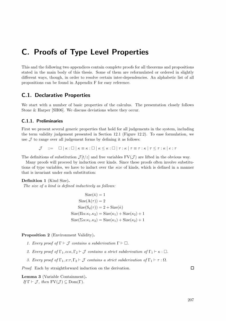
C. Proofs of Type Level Properties
This and the following two appendices contain complete proofs for all theorems and propositionsstated in the main body of this thesis. Some of them are reformulated or ordered in slightlydifferent ways, though, in order to resolve certain inter-dependencies. An alphabetic list of allpropositions can be found in Appendix F for easy reference.
C.1. Declarative Properties
We start with a number of basic properties of the calculus. The presentation closely followsStone & Harper [SH06]. We discuss deviations where they occur.
C.1.1. Preliminaries
First we present several generic properties that hold for all judgements in the system, includingthe term validity judgement presented in Section 12.1 (Figure 12.2). To ease formulation, weuse J to range over all judgement forms by defining it as follows:
J ::= | κ : | κ ≡ κ : | κ ≤ κ : | τ : κ | τ ≡ τ : κ | τ ≤ τ : κ | e : τ
The definitions of substitution J [t/z] and free variables FV(J ) are lifted in the obvious way.Many proofs will proceed by induction over kinds. Since these proofs often involve substitu-
tions of type variables, we have to induct over the size of kinds, which is defined in a mannerthat is invariant under such substitution:
Definition 1 (Kind Size).The size of a kind is defined inductively as follows:
Size(κ) = 1
Size(A(τ)) = 2
Size(Sκ(τ)) = 2 + Size(κ)
Size(Πα:κ1.κ2) = Size(κ1) + Size(κ2) + 1
Size(Σα:κ1.κ2) = Size(κ1) + Size(κ2) + 1
Proposition 2 (Environment Validity).
1. Every proof of Γ ⊢ J contains a subderivation Γ ⊢ .
2. Every proof of Γ1, α:κ,Γ2 ⊢ J contains a strict subderivation of Γ1 ⊢ κ : .
3. Every proof of Γ1, x:τ,Γ2 ⊢ J contains a strict subderivation of Γ1 ⊢ τ : Ω.
Proof. Each by straightforward induction on the derivation.
Lemma 3 (Variable Containment).If Γ ⊢ J , then FV(J ) ⊆ Dom(Γ).
207
C. Proofs of Type Level Properties
Proof. By straightforward induction on the derivation, using Environment Validity in case ofbinders and variables.
Proposition 4 (Reflexivity).
1. If Γ ⊢ κ : , then Γ ⊢ κ ≡ κ′ : .
2. If Γ ⊢ κ : , then Γ ⊢ κ ≤ κ′ : .
3. If Γ ⊢ τ : κ, then Γ ⊢ τ ≡ τ ′ : κ.
4. If Γ ⊢ τ : κ, then Γ ⊢ τ ≤ τ ′ : κ.
Proof. (1)–(3) by straightforward simultaneous induction on the derivation, using EnvironmentValidity in case of binders; (4) trivially by rule TSequiv, using (3).
Lemma 5 (Renaming).
1. If Γ1, α:κ,Γ2 ⊢ J , then there is a derivation of equal structure of Γ1, α′:κ,Γ[α′/α] ⊢
J [α′/α] for every α′ /∈ Dom(Γ1) ∪ Dom(Γ2).
2. If Γ1, x:τ,Γ2 ⊢ J , then there is a derivation of equal structure of Γ1, x′:τ,Γ[x′/x] ⊢ J [x′/x]
for every x′ /∈ Dom(Γ1) ∪ Dom(Γ2).
Proof. Each by straightforward induction on the derivation.
Lemma 6 (Weakening).
1. If Γ ⊢ J and Γ′ ⊢ such that Γ ⊆ Γ′, then Γ′ ⊢ J .
2. If Γ1, α:κ,Γ2 ⊢ J and Γ1 ⊢ κ′ : such that Γ1 ⊢ κ′ ≤ κ : , then Γ1, α:κ′,Γ2 ⊢ J .
3. If Γ1, x:τ,Γ2 ⊢ J and Γ1 ⊢ τ ′ : such that Γ1 ⊢ τ ′ ≤ τ : , then Γ1, x:τ′,Γ2 ⊢ J .
Proof. Each by straightforward induction on the derivation, using Renaming.
Lemma 7 (Environment Modification).
1. If Γ, α:κ ⊢ and Γ ⊢ κ′ : , then Γ, α:κ′ ⊢ .
2. If Γ, α:κ ⊢ J and Γ ⊢ κ′ : and α′ /∈ Dom(Γ, α:κ), then Γ, α:κ′, α′:κ ⊢ J [α′/α].
Proof. Straightforward, using Weakening and Renaming.
We define two auxiliary judgements on substitutions as follows:
Definition 2 (Substitution Validity).The judgement Γ′ ⊢ γ : Γ holds if and only if all of the following conditions hold:
1. Γ′ ⊢
2. ∀α ∈ Dom(Γ),Γ′ ⊢ γ(α) : γ(Γ(α)) and γ(α) = τ
3. ∀x ∈ Dom(Γ),Γ′ ⊢ γ(x) : γ(Γ(x))
Definition 3 (Substitution Equivalence).The judgement Γ′ ⊢ γ ≡ γ′ : Γ holds if and only if all of the following conditions hold:
1. Γ′ ⊢ γ : Γ
208
C.1. Declarative Properties
2. Γ′ ⊢ γ′ : Γ
3. ∀α ∈ Dom(Γ),Γ′ ⊢ γ(α) ≡ γ′(α) : γ(Γ(α))
4. ∀x ∈ Dom(Γ),Γ′ ⊢ γ(x) ≡ γ′(x) : γ(Γ(x))
We can now state the following simple facts about substitutions:
Proposition 8 (Substitutability).
1. If Γ ⊢ J and Γ′ ⊢ γ : Γ, then Γ′ ⊢ γ(J ).
2. If Γ1, α:κ,Γ2 ⊢ and Γ1 ⊢ τ : κ, then Γ1,Γ2[τ/α] ⊢ .
Proof. Both by straightforward induction on the derivation. For rule Epsi note that applyinga substitution to a value always produces a value.
Lemma 9 (Substitution Extensibility). If Γ′ ⊢ γ ≡ γ′ : Γ and α /∈ Dom(Γ′) and Γ′ ⊢ γ(κ) ≡γ′(κ) : with Γ′ ⊢ γ(κ) : and Γ′ ⊢ γ′(κ) : , then:
1. Γ′, α:γ(κ) ⊢ γ ∪ [α/α] ≡ γ′ ∪ [α/α] : Γ, α:κ
2. Γ′, α:γ′(κ) ⊢ γ ∪ [α/α] ≡ γ′ ∪ [α/α] : Γ, α:κ.
Proof. Straightforward, using Ntype and Weakening.
For some proofs we need inversion principles on subkinding and on the type validity judgement.The proof of the latter relies on the following simple lemma:
Lemma 10 (Subderivations).
1. Every proof of Γ ⊢ τ1 τ2 : κ contains a strict subderivation Γ ⊢ τ1 : κ1.
2. Every proof of Γ ⊢ τ ·1 : κ contains a strict subderivation Γ ⊢ τ : κ1.
3. Every proof of Γ ⊢ τ ·2 : κ contains a strict subderivation Γ ⊢ τ : κ1.
Proof. By straightforward simultaneous induction on the derivation.
Proposition 11 (Kind Inclusion Inversion). Let Γ ⊢ κ′ ≤ κ : .
1. If κ = Ω, then κ′ = Ω or κ′ = Sκ(τ′).
2. If κ = A(τ), then κ′ = A(τ ′) with Γ ⊢ τ ′ ≡ τ : Ω, or κ′ = SA(τ ′)(τ′′) with Γ ⊢ A(τ ′) ≤ κ : Ω
and Γ ⊢ τ ′′ : A(τ ′).
3. If κ = Sκ(τ), then κ′ = Sκ′(τ ′) with Γ ⊢ κ′ ≤ κ : Ω and Γ ⊢ τ ′ ≡ τ : κ′.
4. If κ = Πα:κ1.κ2, then κ′ = Πα:κ′1.κ′2 with Γ ⊢ κ′1 ≤ κ1 : and Γ, α:κ′1 ⊢ κ2 ≤ κ′2 : .
5. If κ = Σα:κ1.κ2, then κ′ = Σα:κ′1.κ′2 with Γ ⊢ κ1 ≤ κ′1 : and Γ, α:κ1 ⊢ κ2 ≤ κ′2 : .
Proof. By simultaneous induction on the derivation.
Proposition 12 (Type Validity Inversion). Let Γ ⊢ τ : κ.
1. If τ = α, then Γ ⊢ and α ∈ Dom(Γ).
2. If τ = Ψ, then Γ ⊢ .
209
C. Proofs of Type Level Properties
3. If τ = τ1 → τ2, then Γ ⊢ τ1 : Ω and Γ ⊢ τ2 : Ω.
4. If τ = τ1 × τ2, then Γ ⊢ τ1 : Ω and Γ ⊢ τ2 : Ω.
5. If τ = ∀α:κ1.τ2, then Γ, α:κ1 ⊢ τ2 : Ω.
6. If τ = ∃α:κ1.τ2, then Γ, α:κ1 ⊢ τ2 : Ω.
7. If τ = λα:κ1.τ2, then Γ, α:κ1 ⊢ τ2 : κ2.
8. If τ = τ1 τ2, then Γ ⊢ τ1 : Πα:κ2.κ1 and Γ ⊢ τ2 : κ2.
9. If τ = 〈τ1, τ2〉, then Γ ⊢ τ1 : κ1 and Γ ⊢ τ2 : κ2[τ1/α].
10. If τ = τ1·1, then Γ ⊢ τ1 : Σα:κ1.κ2.
11. If τ = τ1·2, then Γ ⊢ τ1 : Σα:κ1.κ2.
Proof. Each by straightforward induction on the derivation, using Subderivations in the case ofrule Text-sigma.
C.1.2. Validity and Functionality
We next show two central invariants of the type system. Validity states that any phrase ap-pearing in a derivable judgement is well-formed. Functionality says that applying equivalentsubstitutions to equivalent phrases yields equivalent phrases. Likewise, any inclusion relationon phrases is maintained by equivalent substitutions.
As in Stone & Harper, the proof has to be broken up by first showing a restricted version ofFunctionality:
Proposition 13 (Simple Functionality). Let Γ′ ⊢ γ ≡ γ′ : Γ.
1. If Γ ⊢ , then Γ′ ⊢ γ′ ≡ γ : Γ.
2. If Γ ⊢ κ : , then Γ′ ⊢ γ(κ) ≡ γ′(κ) : .
3. If Γ ⊢ κ : , then Γ′ ⊢ γ(κ) ≤ γ′(κ) : .
4. If Γ ⊢ τ : κ, then Γ′ ⊢ γ(τ) ≡ γ′(τ) : γ(κ).
5. If Γ ⊢ τ : κ, then Γ′ ⊢ γ(τ) ≤ γ′(τ) : γ(κ).
Proof. By simultaneous induction on the derivations.
1. case Nempty: Γ = ·
– by definition of Substitution Equivalence, Γ′ ⊢ γ : Γ and Γ′ ⊢ γ′ : Γ
– since Dom(Γ) =, trivially ∀α ∈ Dom(Γ),Γ′ ⊢ γ′(α) ≡ γ(α) : and ∀x ∈ Dom(Γ),Γ′ ⊢ γ′(x) ≡ γ(x) : γ′(Γ(x))
– hence Γ′ ⊢ γ′ ≡ γ : Γ
case Ntype: Γ = Γ1, α:κ
– by inversion, Γ1 ⊢ κ :
– by Environment Validity, Γ1 ⊢
– by definition of Substitution Equivalence, Γ′ ⊢ γ ≡ γ′ : Γ1
– by induction, Γ′ ⊢ γ′ ≡ γ : Γ1
– by definition of Substitution Equivalence, Γ′ ⊢ γ(α) ≡ γ′(α) :
210
C.1. Declarative Properties
– by Symmetry, Γ′ ⊢ γ′(α) ≡ γ(α) :
– hence Γ′ ⊢ γ′ ≡ γ : Γ
case Nterm: Γ = Γ1, x:τ
– by inversion, Γ1 ⊢ τ : Ω
– by Environment Validity, Γ1 ⊢
– by definition of Substitution Equivalence, Γ′ ⊢ γ ≡ γ′ : Γ1
– by induction, Γ′ ⊢ γ′ ≡ γ : Γ1
– by definition of Substitution Equivalence, Γ′ ⊢ γ(x) ≡ γ′(x) : γ(τ)
– by Symmetry, Γ′ ⊢ γ′(x) ≡ γ(x) : γ(τ)
– by (a) and induction (3), Γ′ ⊢ γ(τ) ≤ γ′(τ) : Ω
– by Tsub, Γ′ ⊢ γ′(x) ≡ γ(x) : γ′(τ)
– hence Γ′ ⊢ γ′ ≡ γ : Γ
2. case Komega: κ = Ω
– by inversion, Γ ⊢
– by KQomega, Γ ⊢ Ω ≡ Ω :
case Kabs: κ = A(τ)
– by inversion, Γ ⊢ τ : Ω
– by induction, Γ ⊢ γ(τ) ≡ γ′(τ) : Ω
– by KQabs, Γ ⊢ A(γ(τ)) ≡ A(γ′(τ)) :
case Ksing: κ = Sκ(τ)
– by inversion, Γ ⊢ τ : κ
– by induction, Γ ⊢ γ(τ) ≡ γ′(τ) : γ(κ) and Γ ⊢ γ(κ) ≡ γ′(κ) :
– by KQsing, Γ ⊢ Sγ(κ)(γ(τ)) ≡ Sγ′(κ)(γ′(τ)) :
case Kpi: κ = Πα:κ1.κ2
– by inversion, Γ, α:κ1 ⊢ κ2 :
– by Environment Validity, Γ ⊢ κ1 :
– by induction, Γ′ ⊢ γ(κ1) ≡ γ′(κ1) :
– by Substitutability, Γ′ ⊢ γ(κ1) :
– let Γ1 = Γ, α:κ1 and Γ′1 = Γ′, α:γ(κ1)
– by Ntype, Γ′1 ⊢
– let γ1 = γ ∪ [α/α] and γ′1 = γ′ ∪ [α/α]
– by Substitution Extensibility, Γ′1 ⊢ γ1 ≡ γ′1 : Γ1
– by induction, Γ′, α:γ(κ1) ⊢ γ1(κ2) ≡ γ′1(κ2) :
– by KQpi, Γ′ ⊢ Πα:γ(κ1).γ1(κ2) ≡ Πα:γ′(κ1).γ′1(κ2) :
– hence Γ′ ⊢ γ(Πα:κ1.κ2) ≡ γ′(Πα:κ1.κ2) :
case Ksigma: analogous
3. Similarly, using (1) in the contravariant case.
4. case Tvar: τ = α and κ = Γ(α)
– by inversion, Γ ⊢
– by definition of Substitution Equivalence, Γ′ ⊢ γ(α) ≡ γ′(α) : γ(Γ(α))
case Tpsi: τ = Ψ and κ = Ω
– by inversion, Γ ⊢
– by definition of Substitution Equivalence, Γ′ ⊢
– by TQpsi, Γ′ ⊢ Ψ ≡ Ψ : Ω
case Tarrow: τ = τ1 → τ2 and κ = Ω
211
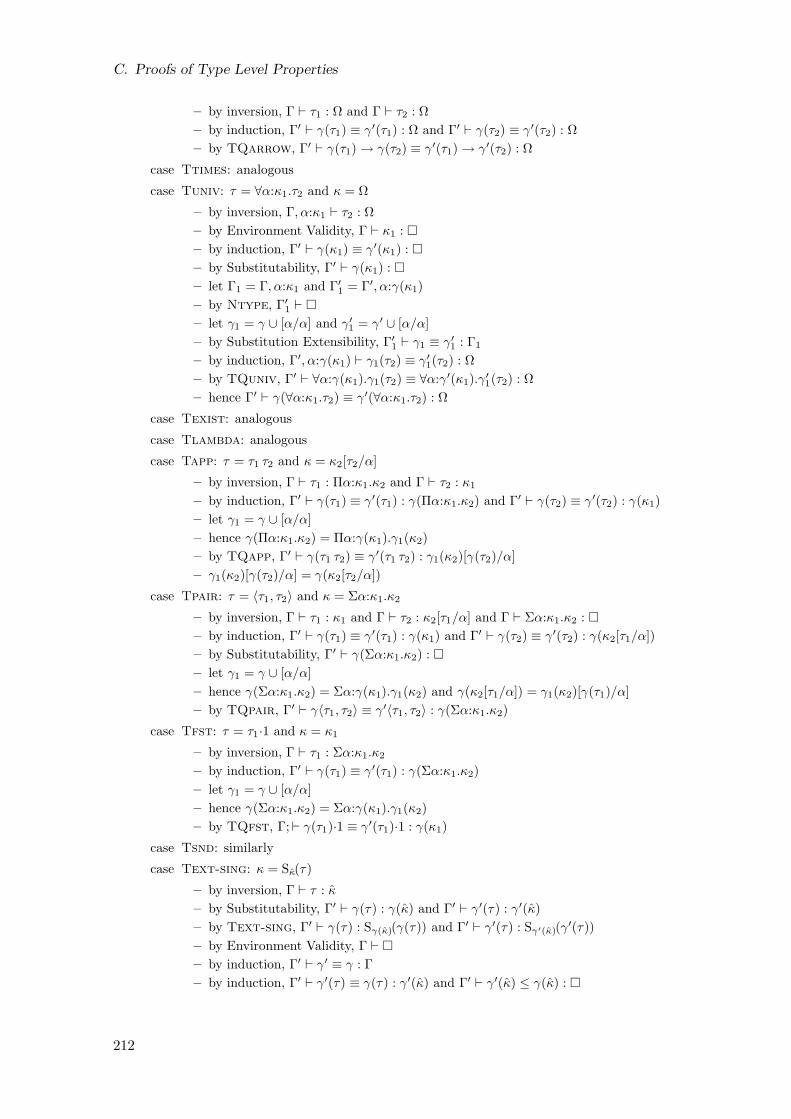
C. Proofs of Type Level Properties
– by inversion, Γ ⊢ τ1 : Ω and Γ ⊢ τ2 : Ω
– by induction, Γ′ ⊢ γ(τ1) ≡ γ′(τ1) : Ω and Γ′ ⊢ γ(τ2) ≡ γ′(τ2) : Ω
– by TQarrow, Γ′ ⊢ γ(τ1) → γ(τ2) ≡ γ′(τ1) → γ′(τ2) : Ω
case Ttimes: analogous
case Tuniv: τ = ∀α:κ1.τ2 and κ = Ω
– by inversion, Γ, α:κ1 ⊢ τ2 : Ω
– by Environment Validity, Γ ⊢ κ1 :
– by induction, Γ′ ⊢ γ(κ1) ≡ γ′(κ1) :
– by Substitutability, Γ′ ⊢ γ(κ1) :
– let Γ1 = Γ, α:κ1 and Γ′1 = Γ′, α:γ(κ1)
– by Ntype, Γ′1 ⊢
– let γ1 = γ ∪ [α/α] and γ′1 = γ′ ∪ [α/α]
– by Substitution Extensibility, Γ′1 ⊢ γ1 ≡ γ′1 : Γ1
– by induction, Γ′, α:γ(κ1) ⊢ γ1(τ2) ≡ γ′1(τ2) : Ω
– by TQuniv, Γ′ ⊢ ∀α:γ(κ1).γ1(τ2) ≡ ∀α:γ′(κ1).γ′1(τ2) : Ω
– hence Γ′ ⊢ γ(∀α:κ1.τ2) ≡ γ′(∀α:κ1.τ2) : Ω
case Texist: analogous
case Tlambda: analogous
case Tapp: τ = τ1 τ2 and κ = κ2[τ2/α]
– by inversion, Γ ⊢ τ1 : Πα:κ1.κ2 and Γ ⊢ τ2 : κ1
– by induction, Γ′ ⊢ γ(τ1) ≡ γ′(τ1) : γ(Πα:κ1.κ2) and Γ′ ⊢ γ(τ2) ≡ γ′(τ2) : γ(κ1)
– let γ1 = γ ∪ [α/α]
– hence γ(Πα:κ1.κ2) = Πα:γ(κ1).γ1(κ2)
– by TQapp, Γ′ ⊢ γ(τ1 τ2) ≡ γ′(τ1 τ2) : γ1(κ2)[γ(τ2)/α]
– γ1(κ2)[γ(τ2)/α] = γ(κ2[τ2/α])
case Tpair: τ = 〈τ1, τ2〉 and κ = Σα:κ1.κ2
– by inversion, Γ ⊢ τ1 : κ1 and Γ ⊢ τ2 : κ2[τ1/α] and Γ ⊢ Σα:κ1.κ2 :
– by induction, Γ′ ⊢ γ(τ1) ≡ γ′(τ1) : γ(κ1) and Γ′ ⊢ γ(τ2) ≡ γ′(τ2) : γ(κ2[τ1/α])
– by Substitutability, Γ′ ⊢ γ(Σα:κ1.κ2) :
– let γ1 = γ ∪ [α/α]
– hence γ(Σα:κ1.κ2) = Σα:γ(κ1).γ1(κ2) and γ(κ2[τ1/α]) = γ1(κ2)[γ(τ1)/α]
– by TQpair, Γ′ ⊢ γ〈τ1, τ2〉 ≡ γ′〈τ1, τ2〉 : γ(Σα:κ1.κ2)
case Tfst: τ = τ1·1 and κ = κ1
– by inversion, Γ ⊢ τ1 : Σα:κ1.κ2
– by induction, Γ′ ⊢ γ(τ1) ≡ γ′(τ1) : γ(Σα:κ1.κ2)
– let γ1 = γ ∪ [α/α]
– hence γ(Σα:κ1.κ2) = Σα:γ(κ1).γ1(κ2)
– by TQfst, Γ;⊢ γ(τ1)·1 ≡ γ′(τ1)·1 : γ(κ1)
case Tsnd: similarly
case Text-sing: κ = Sκ(τ)
– by inversion, Γ ⊢ τ : κ
– by Substitutability, Γ′ ⊢ γ(τ) : γ(κ) and Γ′ ⊢ γ′(τ) : γ′(κ)
– by Text-sing, Γ′ ⊢ γ(τ) : Sγ(κ)(γ(τ)) and Γ′ ⊢ γ′(τ) : Sγ′(κ)(γ′(τ))
– by Environment Validity, Γ ⊢
– by induction, Γ′ ⊢ γ′ ≡ γ : Γ
– by induction, Γ′ ⊢ γ′(τ) ≡ γ(τ) : γ′(κ) and Γ′ ⊢ γ′(κ) ≤ γ(κ) :
212
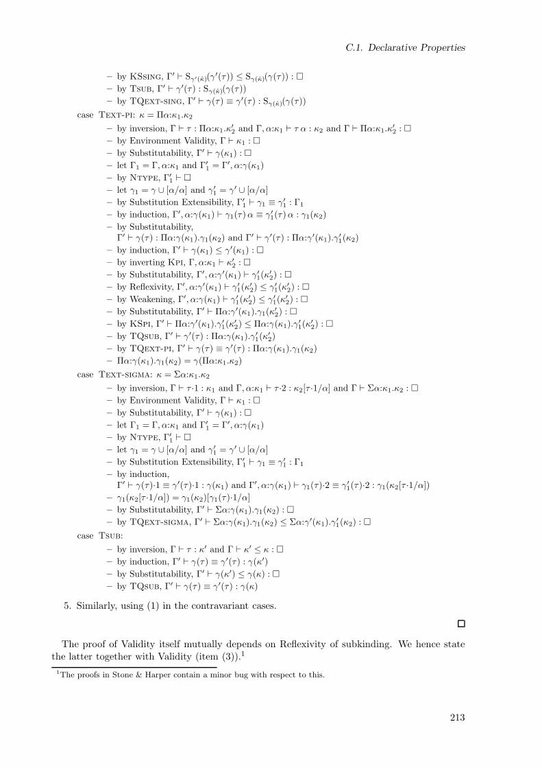
C.1. Declarative Properties
– by KSsing, Γ′ ⊢ Sγ′(κ)(γ′(τ)) ≤ Sγ(κ)(γ(τ)) :
– by Tsub, Γ′ ⊢ γ′(τ) : Sγ(κ)(γ(τ))
– by TQext-sing, Γ′ ⊢ γ(τ) ≡ γ′(τ) : Sγ(κ)(γ(τ))
case Text-pi: κ = Πα:κ1.κ2
– by inversion, Γ ⊢ τ : Πα:κ1.κ′2 and Γ, α:κ1 ⊢ τ α : κ2 and Γ ⊢ Πα:κ1.κ
′2 :
– by Environment Validity, Γ ⊢ κ1 :
– by Substitutability, Γ′ ⊢ γ(κ1) :
– let Γ1 = Γ, α:κ1 and Γ′1 = Γ′, α:γ(κ1)
– by Ntype, Γ′1 ⊢
– let γ1 = γ ∪ [α/α] and γ′1 = γ′ ∪ [α/α]
– by Substitution Extensibility, Γ′1 ⊢ γ1 ≡ γ′1 : Γ1
– by induction, Γ′, α:γ(κ1) ⊢ γ1(τ)α ≡ γ′1(τ)α : γ1(κ2)
– by Substitutability,Γ′ ⊢ γ(τ) : Πα:γ(κ1).γ1(κ2) and Γ′ ⊢ γ′(τ) : Πα:γ′(κ1).γ
′1(κ2)
– by induction, Γ′ ⊢ γ(κ1) ≤ γ′(κ1) :
– by inverting Kpi, Γ, α:κ1 ⊢ κ′2 :
– by Substitutability, Γ′, α:γ′(κ1) ⊢ γ′1(κ′2) :
– by Reflexivity, Γ′, α:γ′(κ1) ⊢ γ′1(κ′2) ≤ γ′1(κ
′2) :
– by Weakening, Γ′, α:γ(κ1) ⊢ γ′1(κ′2) ≤ γ′1(κ
′2) :
– by Substitutability, Γ′ ⊢ Πα:γ′(κ1).γ1(κ′2) :
– by KSpi, Γ′ ⊢ Πα:γ′(κ1).γ′1(κ
′2) ≤ Πα:γ(κ1).γ
′1(κ
′2) :
– by TQsub, Γ′ ⊢ γ′(τ) : Πα:γ(κ1).γ′1(κ
′2)
– by TQext-pi, Γ′ ⊢ γ(τ) ≡ γ′(τ) : Πα:γ(κ1).γ1(κ2)
– Πα:γ(κ1).γ1(κ2) = γ(Πα:κ1.κ2)
case Text-sigma: κ = Σα:κ1.κ2
– by inversion, Γ ⊢ τ ·1 : κ1 and Γ, α:κ1 ⊢ τ ·2 : κ2[τ ·1/α] and Γ ⊢ Σα:κ1.κ2 :
– by Environment Validity, Γ ⊢ κ1 :
– by Substitutability, Γ′ ⊢ γ(κ1) :
– let Γ1 = Γ, α:κ1 and Γ′1 = Γ′, α:γ(κ1)
– by Ntype, Γ′1 ⊢
– let γ1 = γ ∪ [α/α] and γ′1 = γ′ ∪ [α/α]
– by Substitution Extensibility, Γ′1 ⊢ γ1 ≡ γ′1 : Γ1
– by induction,Γ′ ⊢ γ(τ)·1 ≡ γ′(τ)·1 : γ(κ1) and Γ′, α:γ(κ1) ⊢ γ1(τ)·2 ≡ γ′1(τ)·2 : γ1(κ2[τ ·1/α])
– γ1(κ2[τ ·1/α]) = γ1(κ2)[γ1(τ)·1/α]
– by Substitutability, Γ′ ⊢ Σα:γ(κ1).γ1(κ2) :
– by TQext-sigma, Γ′ ⊢ Σα:γ(κ1).γ1(κ2) ≤ Σα:γ′(κ1).γ′1(κ2) :
case Tsub:
– by inversion, Γ ⊢ τ : κ′ and Γ ⊢ κ′ ≤ κ :
– by induction, Γ′ ⊢ γ(τ) ≡ γ′(τ) : γ(κ′)
– by Substitutability, Γ′ ⊢ γ(κ′) ≤ γ(κ) :
– by TQsub, Γ′ ⊢ γ(τ) ≡ γ′(τ) : γ(κ)
5. Similarly, using (1) in the contravariant cases.
The proof of Validity itself mutually depends on Reflexivity of subkinding. We hence statethe latter together with Validity (item (3)).1
1The proofs in Stone & Harper contain a minor bug with respect to this.
213
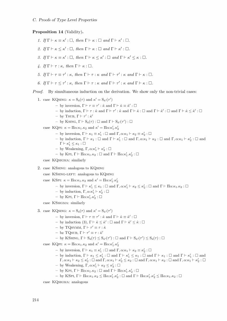
C. Proofs of Type Level Properties
Proposition 14 (Validity).
1. If Γ ⊢ κ ≡ κ′ : , then Γ ⊢ κ : and Γ ⊢ κ′ : .
2. If Γ ⊢ κ ≤ κ′ : , then Γ ⊢ κ : and Γ ⊢ κ′ : .
3. If Γ ⊢ κ ≡ κ′ : , then Γ ⊢ κ ≤ κ′ : and Γ ⊢ κ′ ≤ κ : .
4. If Γ ⊢ τ : κ, then Γ ⊢ κ : .
5. If Γ ⊢ τ ≡ τ ′ : κ, then Γ ⊢ τ : κ and Γ ⊢ τ ′ : κ and Γ ⊢ κ : .
6. If Γ ⊢ τ ≤ τ ′ : κ, then Γ ⊢ τ : κ and Γ ⊢ τ ′ : κ and Γ ⊢ κ : .
Proof. By simultaneous induction on the derivation. We show only the non-trivial cases:
1. case KQsing: κ = Sκ(τ) and κ′ = Sκ′(τ ′)
– by inversion, Γ ⊢ τ ≡ τ ′ : κ and Γ ⊢ κ ≡ κ′ :
– by induction, Γ ⊢ τ : κ and Γ ⊢ τ ′ : κ and Γ ⊢ κ : and Γ ⊢ κ′ : and Γ ⊢ κ ≤ κ′ :
– by Tsub, Γ ⊢ τ ′ : κ′
– by Ksing, Γ ⊢ Sκ(τ) : and Γ ⊢ Sκ′(τ ′) :
case KQpi: κ = Πα:κ1.κ2 and κ′ = Πα:κ′1.κ′2
– by inversion, Γ ⊢ κ1 ≡ κ′1 : and Γ, α:κ1 ⊢ κ2 ≡ κ′2 :
– by induction, Γ ⊢ κ1 : and Γ ⊢ κ′1 : and Γ, α:κ1 ⊢ κ2 : and Γ, α:κ1 ⊢ κ′2 : andΓ ⊢ κ′1 ≤ κ1 :
– by Weakening, Γ, α:κ′1 ⊢ κ′2 :
– by Kpi, Γ ⊢ Πα:κ1.κ2 : and Γ ⊢ Πα:κ′1.κ′2 :
case KQsigma: similarly
2. case KSsing: analogous to KQsing
case KSsing-left: analogous to KQsing
case KSpi: κ = Πα:κ1.κ2 and κ′ = Πα:κ′1.κ′2
– by inversion, Γ ⊢ κ′1 ≤ κ1 : and Γ, α:κ′1 ⊢ κ2 ≤ κ′2 : and Γ ⊢ Πα:κ1.κ2 :
– by induction, Γ, α:κ′1 ⊢ κ′2 :
– by Kpi, Γ ⊢ Πα:κ′1.κ′2 :
case KSsigma: similarly
3. case KQsing: κ = Sκ(τ) and κ′ = Sκ′(τ ′)
– by inversion, Γ ⊢ τ ≡ τ ′ : κ and Γ ⊢ κ ≡ κ′ :
– by induction (3), Γ ⊢ κ ≤ κ′ : and Γ ⊢ κ′ ≤ κ :
– by TQsymm, Γ ⊢ τ ′ ≡ τ : κ
– bz TQsub, Γ ⊢ τ ′ ≡ τ : κ′
– by KSsing, Γ ⊢ Sκ(τ) ≤ Sκ′(τ ′) : and Γ ⊢ Sκ′(τ ′) ≤ Sκ(τ) :
case KQpi: κ = Πα:κ1.κ2 and κ′ = Πα:κ′1.κ′2
– by inversion, Γ ⊢ κ1 ≡ κ′1 : and Γ, α:κ1 ⊢ κ2 ≡ κ′2 :
– by induction, Γ ⊢ κ1 ≤ κ′1 : and Γ ⊢ κ′1 ≤ κ1 : and Γ ⊢ κ1 : and Γ ⊢ κ′1 : andΓ, α:κ1 ⊢ κ2 ≤ κ′2 : and Γ, α:κ1 ⊢ κ′2 ≤ κ2 : and Γ, α:κ1 ⊢ κ2 : and Γ, α:κ1 ⊢ κ′2 :
– by Weakening, Γ, α:κ′1 ⊢ κ2 ≤ κ′2 :
– by Kpi, Γ ⊢ Πα:κ1.κ2 : and Γ ⊢ Πα:κ′1.κ′2 :
– by KSpi, Γ ⊢ Πα:κ1.κ2 ≤ Πα:κ′1.κ′2 : and Γ ⊢ Πα:κ′1.κ
′2 ≤ Πα:κ1.κ2 :
case KQsigma: analogous
214
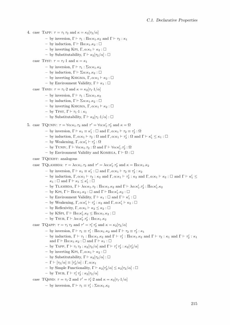
C.1. Declarative Properties
4. case Tapp: τ = τ1 τ2 and κ = κ2[τ2/α]
– by inversion, Γ ⊢ τ1 : Πα:κ1.κ2 and Γ ⊢ τ2 : κ1
– by induction, Γ ⊢ Πα:κ1.κ2 :
– by inverting Kpi, Γ, α:κ1 ⊢ κ2 :
– by Substitutability, Γ ⊢ κ2[τ2/α] :
case Tfst: τ = τ1·1 and κ = κ1
– by inversion, Γ ⊢ τ1 : Σα:κ1.κ2
– by induction, Γ ⊢ Σα:κ1.κ2 :
– by inverting Ksigma, Γ, α:κ1 ⊢ κ2 :
– by Environment Validity, Γ ⊢ κ1 :
case Tsnd: τ = τ1·2 and κ = κ2[τ1·1/α]
– by inversion, Γ ⊢ τ1 : Σα:κ1.κ2
– by induction, Γ ⊢ Σα:κ1.κ2 :
– by inverting Ksigma, Γ, α:κ1 ⊢ κ2 :
– by Tfst, Γ ⊢ τ1·1 : κ1
– by Substitutability, Γ ⊢ κ2[τ1·1/α] :
5. case TQuniv: τ = ∀α:κ1.τ2 and τ ′ = ∀α:κ′1.τ′2 and κ = Ω
– by inversion, Γ ⊢ κ1 ≡ κ′1 : and Γ, α:κ1 ⊢ τ2 ≡ τ ′2 : Ω
– by induction, Γ, α:κ1 ⊢ τ2 : Ω and Γ, α:κ1 ⊢ τ ′2 : Ω and Γ ⊢ κ′1 ≤ κ1 :
– by Weakening, Γ, α:κ′1 ⊢ τ ′2 : Ω
– by Tuniv, Γ ⊢ ∀α:κ1.τ2 : Ω and Γ ⊢ ∀α:κ′1.τ′2 : Ω
– by Environment Validity and Komega, Γ ⊢ Ω :
case TQexist: analogous
case TQlambda: τ = λα:κ1.τ2 and τ ′ = λα:κ′1.τ′2 and κ = Πα:κ1.κ2
– by inversion, Γ ⊢ κ1 ≡ κ′1 : and Γ, α:κ1 ⊢ τ2 ≡ τ ′2 : κ2
– by induction, Γ, α:κ1 ⊢ τ2 : κ2 and Γ, α:κ1 ⊢ τ ′2 : κ2 and Γ, α:κ1 ⊢ κ2 : and Γ ⊢ κ′1 ≤κ1 : and Γ ⊢ κ1 ≤ κ′1 :
– by Tlambda, Γ ⊢ λα:κ1.τ2 : Πα:κ1.κ2 and Γ ⊢ λα:κ′1.τ′2 : Πα:κ′1.κ2
– by Kpi, Γ ⊢ Πα:κ1.κ2 : and Γ ⊢ Πα:κ′1.κ2 :
– by Environment Validity, Γ ⊢ κ1 : and Γ ⊢ κ′1 :
– by Weakening, Γ, α:κ′1 ⊢ τ ′2 : κ2 and Γ, α:κ′1 ⊢ κ2 :
– by Reflexivity, Γ, α:κ1 ⊢ κ2 ≤ κ2 :
– by KSpi, Γ ⊢ Πα:κ′1.κ2 ≤ Πα:κ1.κ2 :
– by Tsub, Γ ⊢ λα:κ′1.τ′2 : Πα:κ1.κ2
case TQapp: τ = τ1 τ2 and τ ′ = τ ′1 τ′2 and κ = κ2[τ2/α]
– by inversion, Γ ⊢ τ1 ≡ τ ′1 : Πα:κ1.κ2 and Γ ⊢ τ2 ≡ τ ′2 : κ1
– by induction, Γ ⊢ τ1 : Πα:κ1.κ2 and Γ ⊢ τ ′1 : Πα:κ1.κ2 and Γ ⊢ τ2 : κ1 and Γ ⊢ τ ′2 : κ1
and Γ ⊢ Πα:κ1.κ2 : and Γ ⊢ κ1 :
– by Tapp, Γ ⊢ τ1 τ2 : κ2[τ2/α] and Γ ⊢ τ ′1 τ′2 : κ2[τ
′2/α]
– by inverting Kpi, Γ, α:κ1 ⊢ κ2 :
– by Substitutability, Γ ⊢ κ2[τ2/α] :
– Γ ⊢ [τ2/α] ≡ [τ ′2/α] : Γ, α:κ1
– by Simple Functionality, Γ ⊢ κ2[τ′2/α] ≤ κ2[τ2/α] :
– by Tsub, Γ ⊢ τ ′1 τ′2 : κ2[τ2/α]
case TQsnd: τ = τ1·2 and τ ′ = τ ′1·2 and κ = κ2[τ1·1/α]
– by inversion, Γ ⊢ τ1 ≡ τ ′1 : Σα:κ1.κ2
215
C. Proofs of Type Level Properties
– by induction, Γ ⊢ τ1 : Σα:κ1.κ2 and Γ ⊢ τ ′1 : Σα:κ1.κ2 and Γ ⊢ Σα:κ1.κ2 :
– by Tsnd, Γ ⊢ τ1·2 : κ2[τ1·1/α] and Γ ⊢ τ ′1·2 : κ2[τ′1·1/α]
– by inverting Ksigma, Γ, α:κ1 ⊢ κ2 :
– by Tfst, Γ ⊢ τ1·1 : κ1 and Γ ⊢ τ ′1·1 : κ1
– by Substitutability, Γ ⊢ κ2[τ1·1/α] :
– by TQfst, Γ ⊢ τ1·1 ≡ τ ′1·1 : κ1
– hence Γ ⊢ [τ1·1/α] ≡ [τ ′1·1/α] : Γ, α:κ1
– by Simple Functionality, Γ ⊢ κ2[τ′1/α] ≤ κ2[τ1/α] :
– by Tsub, Γ ⊢ τ ′1·2 : κ2[τ1·1/α]
case TQext-pi: κ = Πα:κ1.κ2
– by inversion, Γ, α:κ1 ⊢ τ α ≡ τ ′ α : κ2 and Γ ⊢ τ : Πα:κ1.κ′2 and Γ ⊢ τ ′ : Πα:κ1.κ
′′2
– by induction, Γ, α:κ1 ⊢ τ α : κ2 and Γ, α:κ1 ⊢ τ ′ α : κ2 and Γ, α:κ1 ⊢ κ2 : andΓ ⊢ Πα:κ1.κ
′2 : and Γ ⊢ Πα:κ1.κ
′′2 :
– by Text-pi, Γ ⊢ τ : Πα:κ1.κ2 and Γ ⊢ τ ′ : Πα:κ1.κ2
– by Kpi, Γ ⊢ Πα:κ1.κ2 :
case TQext-sigma:
– by inversion, Γ ⊢ τ ·1 ≡ τ ′·1 : κ1 and Γ ⊢ τ ·2 ≡ τ ′·2 : κ2[τ ·1/α] and Γ ⊢ Σα:κ1.κ2 :
– by induction, Γ ⊢ τ ′·1 : κ1 and Γ ⊢ τ ′·2 : κ2[τ ·1/α]
– by Text-sigma, Γ ⊢ τ ′ : Σα:κ1.κ2
6. case TSuniv: τ = ∀α:κ1.τ2 and τ ′ = ∀α:κ′1.τ′2 and κ = Ω
– by inversion, Γ ⊢ κ′1 ≤ κ1 : and Γ, α:κ′1 ⊢ τ2 ≤ τ ′2 : Ω and Γ ⊢ ∀α:κ1.τ2 : Ω
– by induction, Γ, α:κ′1 ⊢ τ ′2 : Ω
– by Tuniv, Γ ⊢ ∀α:κ′1.τ′2 : Ω
– by Environment Validity and Komega, Γ ⊢ Ω :
case TSexist: similarly.
Given Validity, we can easily prove symmetry and transitivity properties:
Proposition 15 (Antisymmetry of Kind Inclusion). If and only if Γ ⊢ κ ≤ κ′ : andΓ ⊢ κ′ ≤ κ : , then Γ ⊢ κ ≡ κ′ : .
Proof. The inverse direction has already been shown as Validity (3). The other is shown byinduction on the added size of both derivations. The only cases possible are those where bothderivations used the same rule:
case KSomega: κ = κ′ = Ω
– by inversion, Γ ⊢
– by KQomega, Γ ⊢ Ω ≡ Ω :
case KSabs: κ = A(τ) and κ′ = A(τ ′)
– by inversion, Γ ⊢ τ ≡ τ ′ : Ω
– by KQabs, Γ ⊢ A(τ) ≡ A(τ ′) :
case KSsing: κ = Sκ(τ) and κ′ = Sκ′(τ ′)
– by inversion, Γ ⊢ τ ≡ τ ′ : κ and Γ ⊢ κ ≤ κ′ : and Γ ⊢ κ′ ≤ κ :
– by induction, Γ ⊢ κ ≡ κ′ :
216
C.1. Declarative Properties
– by KQsing, Γ ⊢ Sκ(τ) ≡ Sκ′(τ ′) :
case KSpi: κ = Πα:κ1.κ2 and κ′ = Πα:κ′1.κ′2
– by inversion, Γ ⊢ κ′1 ≤ κ1 : and Γ, α:κ′1 ⊢ κ2 ≤ κ′2 : and Γ ⊢ κ′1 ≤ κ1 : andΓ, α:κ1 ⊢ κ′2 ≤ κ2 :
– by induction, Γ ⊢ κ1 ≡ κ′1 : and Γ, α:κ′1 ⊢ κ2 ≡ κ′2 :
– by Environment Validity, Γ ⊢ κ1 :
– by Weakening, Γ, α:κ1 ⊢ κ2 ≡ κ′2 :
– by KQpi, Γ ⊢ Πα:κ1.κ2 ≡ Πα:κ′1.κ′2 :
case KSsigma: analogous
Proposition 16 (Symmetry).
1. If Γ ⊢ κ ≡ κ′ : , then Γ ⊢ κ′ ≡ κ : .
2. If Γ ⊢ τ ≡ τ ′ : κ, then Γ ⊢ τ ′ ≡ τ : κ.
Proof.
1. By easy induction on the derivation.
2. Trivial, by Rule TQsymm.
Proposition 17 (Transitivity).
1. If Γ ⊢ κ ≡ κ′ : and Γ ⊢ κ′ ≡ κ′′ : , then Γ ⊢ κ ≡ κ′′ : .
2. If Γ ⊢ κ ≤ κ′ : and Γ ⊢ κ′ ≤ κ′′ : , then Γ ⊢ κ ≤ κ′′ : .
3. If Γ ⊢ τ ≡ τ ′ : κ and Γ ⊢ τ ′ ≡ τ ′′ : κ, then Γ ⊢ τ ≡ τ ′′ : κ.
4. If Γ ⊢ τ ≤ τ ′ : κ and Γ ⊢ τ ′ ≤ τ ′′ : κ, then Γ ⊢ τ ≤ τ ′′ : κ.
Proof.
1. By straightforward induction on Size(κ)+Size(κ′)+Size(κ′′), using (3) in case of singletonsand abstraction types, and Antisymmetry and Weakening in case of binders.
2. Similarly.
3. Trivially by rule TQtrans.
4. Trivially by rule TStrans.
This gives us the necessary prerequisites for proving Functionality in its final formulation:
Proposition 18 (Full Functionality). Let Γ′ ⊢ γ ≡ γ′ : Γ.
1. If Γ ⊢ κ ≡ κ′ : , then Γ′ ⊢ γ(κ) ≡ γ′(κ′) : .
2. If Γ ⊢ κ ≤ κ′ : , then Γ′ ⊢ γ(κ) ≤ γ′(κ′) : .
217
C. Proofs of Type Level Properties
3. If Γ ⊢ τ ≡ τ ′ : κ, then Γ′ ⊢ γ(τ) ≡ γ′(τ ′) : γ(κ).
4. If Γ ⊢ τ ≤ τ ′ : κ, then Γ′ ⊢ γ(τ) ≤ γ′(τ ′) : γ(κ).
Proof. Each by induction on the derivation:
1. • by Substitutability, Γ′ ⊢ γ(κ) ≡ γ(κ′) :
• by Validity, Γ ⊢ κ′ :
• by Simple Functionality, Γ′ ⊢ γ(κ′) ≡ γ′(κ′) :
• by Transitivity, Γ′ ⊢ γ(κ) ≡ γ′(κ′) :
2–4. Likewise.
C.2. Derivable Rules
C.2.1. Higher-Order Singletons
With Validity and Functionality proven in the previous section, we are now prepared to showthe admissibility of the derived rules for higher-order singletons (Figure 11.9) and for βη-equivalences. We just need another trivial lemma:
Lemma 19 (Kind Subsumption).
1. If Γ ⊢ τ : A(τ1), then Γ ⊢ τ : Ω.
2. If Γ ⊢ τ : Sκ(τ1), then Γ ⊢ τ : κ.
3. If Γ ⊢ τ ≡ τ ′ : A(τ1), then Γ ⊢ τ ≡ τ ′ : Ω.
4. If Γ ⊢ τ ≡ τ ′ : Sκ(τ1), then Γ ⊢ τ ≡ τ ′ : κ.
5. If Γ ⊢ τ ≤ τ ′ : A(τ1), then Γ ⊢ τ ≤ τ ′ : Ω.
6. If Γ ⊢ τ ≤ τ ′ : Sκ(τ1), then Γ ⊢ τ ≤ τ ′ : κ.
Proof. Straightforward, using Validity.
Theorem 20 (Admissibility of Higher-Order Singleton Rules).The rules Ksing*, Text-sing, KQsing*, KSsing*, KSsing-left* and TQext-sing* are deriv-
able.
Proof.
1. KQsing*: By induction on the size of κ.
case κ = Ω:
– by inverting KQomega, κ′ = Ω
– by KQsing, Γ ⊢ SΩ(τ) ≡ SΩ(τ ′) :
case κ = A(τ1):
– by inverting KQabs, κ′ = A(τ ′1)
– by KQsing, Γ ⊢ SA(τ1)(τ) ≡ SA(τ ′1)(τ ′) :
case κ = Sκ(τ1):
218
C.2. Derivable Rules
– by inverting KQsing, κ′ = Sκ′(τ ′1)
– by premise, Γ ⊢ Sκ(τ1) ≡ Sκ′(τ ′1) :
case κ = Πα:κ1.κ2:
– by inverting KQpi,κ′ = Πα:κ′1.κ
′2 and Γ ⊢ κ1 ≡ κ′1 : and Γ, α:κ1 ⊢ κ2 ≡ κ′2 :
– by Environment Validity, Γ, α:κ1 ⊢
– by Weakening, Γ, α:κ1 ⊢ τ ≡ τ ′ : Πα:κ1.κ2
– by TQvar, Γ, α:κ1 ⊢ α ≡ α : κ1
– by TQapp, Γ, α:κ1 ⊢ τ α ≡ τ ′ α : κ2
– by induction, Γ, α:κ1 ⊢ S(τ α : κ2) ≡ S(τ ′ α : κ′2) :
– by KQpi, Γ ⊢ Πα:κ1.S(τ α : κ2) ≡ Πα:κ1.S(τ α : κ′2) :
case κ = Σα:κ1.κ2:
– by Validity, Γ ⊢ Σα:κ1.κ2 :
– by inverting KQsigma,κ′ = Σα:κ′1.κ
′2 and Γ ⊢ κ1 ≡ κ′1 : and Γ, α:κ1 ⊢ κ2 ≡ κ′2 :
– by Environment Validity, Γ, α:κ1 ⊢
– by TQfst, Γ ⊢ τ ·1 ≡ τ ′·1 : κ1
– by TQsnd, Γ ⊢ τ ·2 ≡ τ ′·2 : κ2[τ ·1/α]
– obviously, Γ ⊢ [τ ·1/α] ≡ [τ ′·1/α] : Γ, α:κ1
– by Full Functionality, Γ ⊢ κ2[τ ·1/α] ≡ κ′2[τ′·1/α] :
– by induction, Γ ⊢ S(τ ·1 : κ1) ≡ S(τ ′·1 : κ′1) : and Γ ⊢ S(τ ·2 : κ2[τ ·1/α]) ≡ S(τ ′·2 : κ′2[τ
′·1/α]) :
– by Weakening, Γ, α:κ1 ⊢ S(τ ·2 : κ2[τ ·1/α]) ≡ S(τ ′·2 : κ′2[τ′·1/α]) :
– by KQsigma,Γ ⊢ S(τ ·1 : κ1) × S(τ ·2 : κ2[τ ·1/α]) ≡ S(τ ′·1 : κ′1) × S(τ ′·2 : κ′2[τ
′·1/α]) :
2. KSsing*: similarly, but with a case distinction for abstraction kinds and singletons:
case κ = A(τ1): case distinction for κ′:
subcase κ′ = Ω (by KSabs-left):
∗ by KSsing, Γ ⊢ SA(τ1)(τ) ≤ SΩ(τ ′) :
subcase κ′ = A(τ ′1) (by KSabs):
∗ by KSsing, Γ ⊢ SA(τ1)(τ) ≤ SA(τ ′1)(τ ′) :
case κ = Sκ(τ1): case distinction for κ′:
subcase κ′ = κ′ (by KSsing-left):
∗ by inverting KSsing-left, Γ ⊢ κ ≤ κ′ :
∗ by inverting Ksing, Γ ⊢ τ1 : κ
∗ by Text-sing, Γ ⊢ τ1 : Sκ(τ1)
∗ by Validity, Γ ⊢ τ1 : Sκ(τ1)
∗ by TQext-sing, Γ ⊢ τ1 ≡ τ ′ : Sκ(τ1)
∗ by Kind Subsumption, Γ ⊢ τ1 ≡ τ ′ : κ
∗ by KSsing, Γ ⊢ Sκ(τ1) ≤ Sκ′(τ ′) :
subcase κ′ = Sκ′(τ ′1) (by KSsing):
∗ by premise, Γ ⊢ Sκ(τ1) ≤ Sκ′(τ ′1) :
3. KSsing-left*: by induction on the size of κ:
case κ = κ:
– by KSsing-left, Γ ⊢ Sκ(τ) ≤ κ :
219
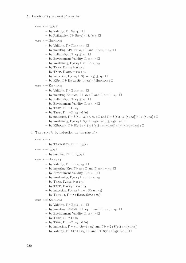
C. Proofs of Type Level Properties
case κ = Sκ(τ1):
– by Validity, Γ ⊢ Sκ(τ1) :
– by Reflexivity, Γ ⊢ Sκ(τ1) ≤ Sκ(τ1) :
case κ = Πα:κ1.κ2:
– by Validity, Γ ⊢ Πα:κ1.κ2 :
– by inverting Kpi, Γ ⊢ κ1 : and Γ, α:κ1 ⊢ κ2 :
– by Reflexivity, Γ ⊢ κ1 ≤ κ1 :
– by Environment Validity, Γ, α:κ1 ⊢
– by Weakening, Γ, α:κ1 ⊢ τ : Πα:κ1.κ2
– by Tvar, Γ, α:κ1 ⊢ α : κ1
– by Tapp, Γ, α:κ1 ⊢ τ α : κ2
– by induction, Γ, α:κ1 ⊢ S(τ α : κ2) ≤ κ2 :
– by KSpi, Γ ⊢ Πα:κ1.S(τ α : κ2) ≤ Πα:κ1.κ2 :
case κ = Σα:κ1.κ2:
– by Validity, Γ ⊢ Σα:κ1.κ2 :
– by inverting Ksigma, Γ ⊢ κ1 : and Γ, α:κ1 ⊢ κ2 :
– by Reflexivity, Γ ⊢ κ1 ≤ κ1 :
– by Environment Validity, Γ, α:κ1 ⊢
– by Tfst, Γ ⊢ τ ·1 : κ1
– by Tsnd, Γ ⊢ τ ·2 : κ2[τ ·1/α]
– by induction, Γ ⊢ S(τ ·1 : κ1) ≤ κ1 : and Γ ⊢ S(τ ·2 : κ2[τ ·1/α]) ≤ κ2[τ ·1/α] :
– by Weakening, Γ, α:κ1 ⊢ S(τ ·2 : κ2[τ ·1/α]) ≤ κ2[τ ·1/α] :
– by KSsigma, Γ ⊢ S(τ ·1 : κ1) × S(τ ·2 : κ2[τ ·1/α]) ≤ κ1 × κ2[τ ·1/α] :
4. Text-sing*: by induction on the size of κ:
case κ = κ:
– by Text-sing, Γ ⊢ τ : Sκ(τ)
case κ = Sκ(τ1):
– by premise, Γ ⊢ τ : Sκ(τ1)
case κ = Πα:κ1.κ2:
– by Validity, Γ ⊢ Πα:κ1.κ2 :
– by inverting Kpi, Γ ⊢ κ1 : and Γ, α:κ1 ⊢ κ2 :
– by Environment Validity, Γ, α:κ1 ⊢
– by Weakening, Γ, α:κ1 ⊢ τ : Πα:κ1.κ2
– by Tvar, Γ, α:κ1 ⊢ α : κ1
– by Tapp, Γ, α:κ1 ⊢ τ α : κ2
– by induction, Γ, α:κ1 ⊢ τ α : S(τ α : κ2)
– by Text-pi, Γ ⊢ τ : Πα:κ1.S(τ α : κ2)
case κ = Σα:κ1.κ2:
– by Validity, Γ ⊢ Σα:κ1.κ2 :
– by inverting Ksigma, Γ ⊢ κ1 : and Γ, α:κ1 ⊢ κ2 :
– by Environment Validity, Γ, α:κ1 ⊢
– by Tfst, Γ ⊢ τ ·1 : κ1
– by Tsnd, Γ ⊢ τ ·2 : κ2[τ ·1/α]
– by induction, Γ ⊢ τ ·1 : S(τ ·1 : κ1) and Γ ⊢ τ ·2 : S(τ ·2 : κ2[τ ·1/α])
– by Validity, Γ ⊢ S(τ ·1 : κ1) : and Γ ⊢ S(τ ·2 : κ2[τ ·1/α]) :
220
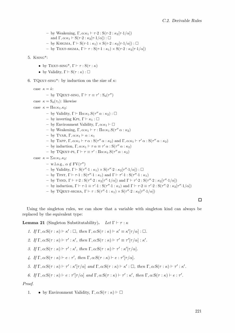
C.2. Derivable Rules
– by Weakening, Γ, α:κ1 ⊢ τ ·2 : S(τ ·2 : κ2[τ ·1/α])and Γ, α:κ1 ⊢ S(τ ·2 : κ2[τ ·1/α]) :
– by Ksigma, Γ ⊢ S(τ ·1 : κ1) × S(τ ·2 : κ2[τ ·1/α]) :
– by Text-sigma, Γ ⊢ τ : S(τ ·1 : κ1) × S(τ ·2 : κ2[τ ·1/α])
5. Ksing*:
• by Text-sing*, Γ ⊢ τ : S(τ : κ)
• by Validity, Γ ⊢ S(τ : κ) :
6. TQext-sing*: by induction on the size of κ:
case κ = κ:
– by TQext-sing, Γ ⊢ τ ≡ τ ′ : Sκ(τ′′)
case κ = Sκ(τ1): likewise
case κ = Πα:κ1.κ2:
– by Validity, Γ ⊢ Πα:κ1.S(τ ′′ α : κ2) :
– by inverting Kpi, Γ ⊢ κ1 :
– by Environment Validity, Γ, α:κ1 ⊢
– by Weakening, Γ, α:κ1 ⊢ τ : Πα:κ1.S(τ ′′ α : κ2)
– by Tvar, Γ, α:κ1 ⊢ α : κ1
– by Tapp, Γ, α:κ1 ⊢ τ α : S(τ ′′ α : κ2) and Γ, α:κ1 ⊢ τ ′ α : S(τ ′′ α : κ2)
– by induction, Γ, α:κ1 ⊢ τ α ≡ τ ′ α : S(τ ′′ α : κ2)
– by TQext-pi, Γ ⊢ τ ≡ τ ′ : Πα:κ1.S(τ ′′ α : κ2)
case κ = Σα:κ1.κ2:
– w.l.o.g., α /∈ FV(τ ′′)
– by Validity, Γ ⊢ S(τ ′′·1 : κ1) × S(τ ′′·2 : κ2[τ′′·1/α]) :
– by Tfst, Γ ⊢ τ ·1 : S(τ ′′·1 : κ1) and Γ ⊢ τ ′·1 : S(τ ′′·1 : κ1)
– by Tsnd, Γ ⊢ τ ·2 : S(τ ′′·2 : κ2[τ′′·1/α]) and Γ ⊢ τ ′·2 : S(τ ′′·2 : κ2[τ
′′·1/α])
– by induction, Γ ⊢ τ ·1 ≡ τ ′·1 : S(τ ′′·1 : κ1) and Γ ⊢ τ ·2 ≡ τ ′·2 : S(τ ′′·2 : κ2[τ′′·1/α])
– by TQext-sigma, Γ ⊢ τ : S(τ ′′·1 : κ1) × S(τ ′′·2 : κ2[τ′′·1/α])
Using the singleton rules, we can show that a variable with singleton kind can always bereplaced by the equivalent type:
Lemma 21 (Singleton Substitutability). Let Γ ⊢ τ : κ
1. If Γ, α:S(τ : κ) ⊢ κ′ : , then Γ, α:S(τ : κ) ⊢ κ′ ≡ κ′[τ/α] : .
2. If Γ, α:S(τ : κ) ⊢ τ ′ : κ′, then Γ, α:S(τ : κ) ⊢ τ ′ ≡ τ ′[τ/α] : κ′.
3. If Γ, α:S(τ : κ) ⊢ τ ′ : κ′, then Γ, α:S(τ : κ) ⊢ τ ′ : κ′[τ/α].
4. If Γ, α:S(τ : κ) ⊢ e : τ ′, then Γ, α:S(τ : κ) ⊢ e : τ ′[τ/α].
5. If Γ, α:S(τ : κ) ⊢ τ ′ : κ′[τ/α] and Γ, α:S(τ : κ) ⊢ κ′ : , then Γ, α:S(τ : κ) ⊢ τ ′ : κ′.
6. If Γ, α:S(τ : κ) ⊢ e : τ ′[τ/α] and Γ, α:S(τ : κ) ⊢ τ ′ : κ′, then Γ, α:S(τ : κ) ⊢ e : τ ′.
Proof.
1. • by Environment Validity, Γ, α:S(τ : κ) ⊢
221
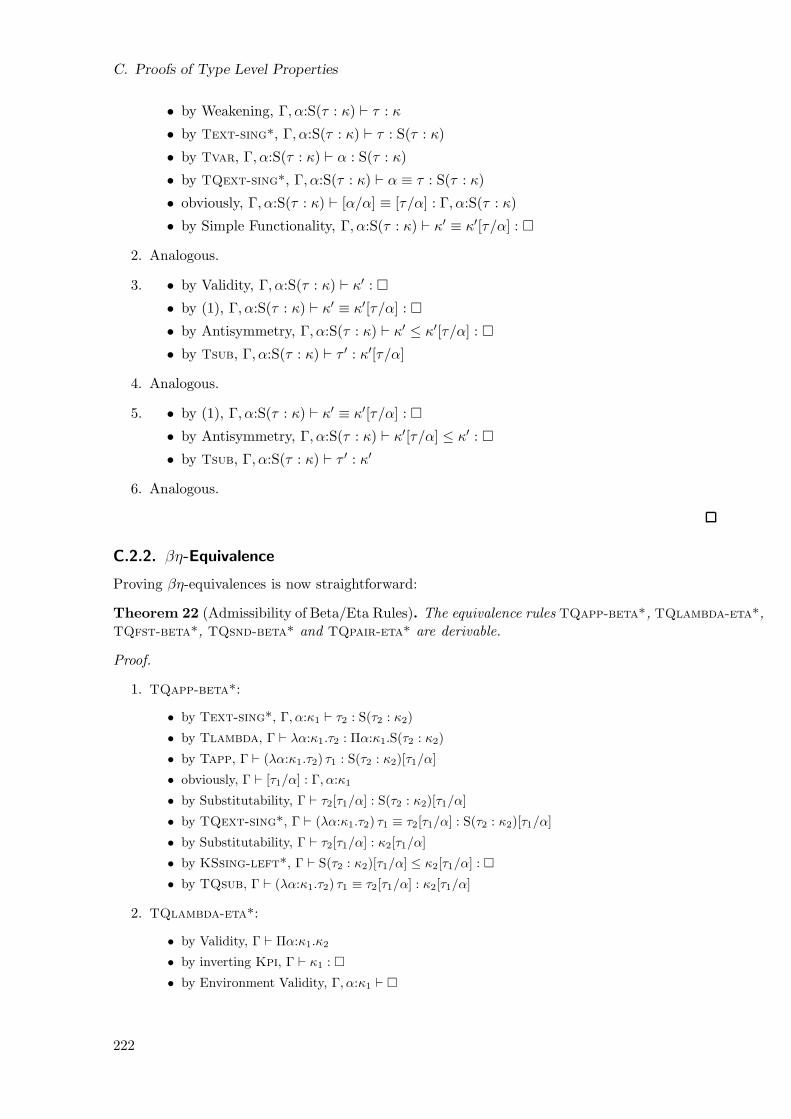
C. Proofs of Type Level Properties
• by Weakening, Γ, α:S(τ : κ) ⊢ τ : κ
• by Text-sing*, Γ, α:S(τ : κ) ⊢ τ : S(τ : κ)
• by Tvar, Γ, α:S(τ : κ) ⊢ α : S(τ : κ)
• by TQext-sing*, Γ, α:S(τ : κ) ⊢ α ≡ τ : S(τ : κ)
• obviously, Γ, α:S(τ : κ) ⊢ [α/α] ≡ [τ/α] : Γ, α:S(τ : κ)
• by Simple Functionality, Γ, α:S(τ : κ) ⊢ κ′ ≡ κ′[τ/α] :
2. Analogous.
3. • by Validity, Γ, α:S(τ : κ) ⊢ κ′ :
• by (1), Γ, α:S(τ : κ) ⊢ κ′ ≡ κ′[τ/α] :
• by Antisymmetry, Γ, α:S(τ : κ) ⊢ κ′ ≤ κ′[τ/α] :
• by Tsub, Γ, α:S(τ : κ) ⊢ τ ′ : κ′[τ/α]
4. Analogous.
5. • by (1), Γ, α:S(τ : κ) ⊢ κ′ ≡ κ′[τ/α] :
• by Antisymmetry, Γ, α:S(τ : κ) ⊢ κ′[τ/α] ≤ κ′ :
• by Tsub, Γ, α:S(τ : κ) ⊢ τ ′ : κ′
6. Analogous.
C.2.2. βη-Equivalence
Proving βη-equivalences is now straightforward:
Theorem 22 (Admissibility of Beta/Eta Rules). The equivalence rules TQapp-beta*, TQlambda-eta*,TQfst-beta*, TQsnd-beta* and TQpair-eta* are derivable.
Proof.
1. TQapp-beta*:
• by Text-sing*, Γ, α:κ1 ⊢ τ2 : S(τ2 : κ2)
• by Tlambda, Γ ⊢ λα:κ1.τ2 : Πα:κ1.S(τ2 : κ2)
• by Tapp, Γ ⊢ (λα:κ1.τ2) τ1 : S(τ2 : κ2)[τ1/α]
• obviously, Γ ⊢ [τ1/α] : Γ, α:κ1
• by Substitutability, Γ ⊢ τ2[τ1/α] : S(τ2 : κ2)[τ1/α]
• by TQext-sing*, Γ ⊢ (λα:κ1.τ2) τ1 ≡ τ2[τ1/α] : S(τ2 : κ2)[τ1/α]
• by Substitutability, Γ ⊢ τ2[τ1/α] : κ2[τ1/α]
• by KSsing-left*, Γ ⊢ S(τ2 : κ2)[τ1/α] ≤ κ2[τ1/α] :
• by TQsub, Γ ⊢ (λα:κ1.τ2) τ1 ≡ τ2[τ1/α] : κ2[τ1/α]
2. TQlambda-eta*:
• by Validity, Γ ⊢ Πα:κ1.κ2
• by inverting Kpi, Γ ⊢ κ1 :
• by Environment Validity, Γ, α:κ1 ⊢
222
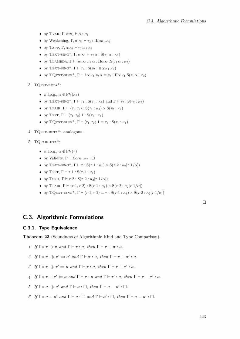
C.3. Algorithmic Formulations
• by Tvar, Γ, α:κ1 ⊢ α : κ1
• by Weakening, Γ, α:κ1 ⊢ τ2 : Πα:κ1.κ2
• by Tapp, Γ, α:κ1 ⊢ τ2 α : κ2
• by Text-sing*, Γ, α:κ1 ⊢ τ2 α : S(τ1 α : κ2)
• by Tlambda, Γ ⊢ λα:κ1.τ2 α : Πα:κ1.S(τ1 α : κ2)
• by Text-sing*, Γ ⊢ τ2 : S(τ2 : Πα:κ1.κ2)
• by TQext-sing*, Γ ⊢ λα:κ1.τ2 α ≡ τ2 : Πα:κ1.S(τ1 α : κ2)
3. TQfst-beta*:
• w.l.o.g., α /∈ FV(κ2)
• by Text-sing*, Γ ⊢ τ1 : S(τ1 : κ1) and Γ ⊢ τ2 : S(τ2 : κ2)
• by Tpair, Γ ⊢ 〈τ1, τ2〉 : S(τ1 : κ1) × S(τ2 : κ2)
• by Tfst, Γ ⊢ 〈τ1, τ2〉·1 : S(τ1 : κ1)
• by TQext-sing*, Γ ⊢ 〈τ1, τ2〉·1 ≡ τ1 : S(τ1 : κ1)
4. TQsnd-beta*: analogous.
5. TQpair-eta*:
• w.l.o.g., α /∈ FV(τ)
• by Validity, Γ ⊢ Σα:κ1.κ2 :
• by Text-sing*, Γ ⊢ τ : S(τ ·1 : κ1) × S(τ ·2 : κ2[τ ·1/α])
• by Tfst, Γ ⊢ τ ·1 : S(τ ·1 : κ1)
• by Tsnd, Γ ⊢ τ ·2 : S(τ ·2 : κ2[τ ·1/α])
• by Tpair, Γ ⊢ 〈τ ·1, τ ·2〉 : S(τ ·1 : κ1) × S(τ ·2 : κ2[τ ·1/α])
• by TQext-sing*, Γ ⊢ 〈τ ·1, τ ·2〉 ≡ τ : S(τ ·1 : κ1) × S(τ ·2 : κ2[τ ·1/α])
C.3. Algorithmic Formulations
C.3.1. Type Equivalence
Theorem 23 (Soundness of Algorithmic Kind and Type Comparison).
1. If Γ ⊲ τ π and Γ ⊢ τ : κ, then Γ ⊢ τ ≡ π : κ.
2. If Γ ⊲ π π′ κ′ and Γ ⊢ π : κ, then Γ ⊢ π ≡ π′ : κ.
3. If Γ ⊲ τ τ ′ κ and Γ ⊢ τ : κ, then Γ ⊢ τ ≡ τ ′ : κ.
4. If Γ ⊲ τ ≡ τ ′ κ and Γ ⊢ τ : κ and Γ ⊢ τ ′ : κ, then Γ ⊢ τ ≡ τ ′ : κ.
5. If Γ ⊲ κ κ′ and Γ ⊢ κ : , then Γ ⊢ κ ≡ κ′ : .
6. If Γ ⊲ κ ≡ κ′ and Γ ⊢ κ : and Γ ⊢ κ′ : , then Γ ⊢ κ ≡ κ′ : .
223
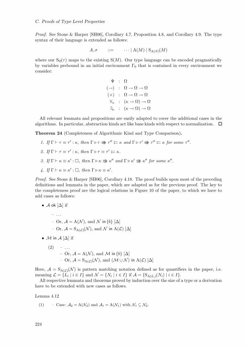
C. Proofs of Type Level Properties
Proof. See Stone & Harper [SH06], Corollary 4.7, Proposition 4.8, and Corollary 4.9. The typesyntax of their language is extended as follows:
A,σ ::= · · · | A(M) | SA(N)(M)
where our SΩ(τ) maps to the existing S(M). Our type language can be encoded pragmaticallyby variables prebound in an initial environment Γ0 that is contained in every environment weconsider:
Ψ : Ω
(→) : Ω → Ω → Ω
(×) : Ω → Ω → Ω
∀κ : (κ→ Ω) → Ω
∃κ : (κ→ Ω) → Ω
All relevant lemmata and propositions are easily adapted to cover the additional cases in thealgorithms. In particular, abstraction kinds act like base kinds with respect to normalization.
Theorem 24 (Completeness of Algorithmic Kind and Type Comparison).
1. If Γ ⊢ τ ≡ τ ′ : κ, then Γ ⊲ τ τ ′′ κ and Γ ⊲ τ ′ τ ′′ κ for some τ ′′.
2. If Γ ⊢ τ ≡ τ ′ : κ, then Γ ⊲ τ ≡ τ ′ κ.
3. If Γ ⊢ κ ≡ κ′ : , then Γ ⊲ κ κ′′ and Γ ⊲ κ′ κ′′ for some κ′′.
4. If Γ ⊢ κ ≡ κ′ : , then Γ ⊲ κ ≡ κ′.
Proof. See Stone & Harper [SH06], Corollary 4.18. The proof builds upon most of the precedingdefinitions and lemmata in the paper, which are adapted as for the previous proof. The key tothe completeness proof are the logical relations in Figure 10 of the paper, to which we have toadd cases as follows:
• A ok [∆] if
– . . .
– Or, A = A(N ), and N in b [∆]
– Or, A = SA(L)(N ), and N in A(L) [∆]
• M in A [∆] if
(2) – . . .
– Or, A = A(N ), and M in b [∆]
– Or, A = SA(L)(N ), and (M∪N ) in A(L) [∆]
Here, A = SA(L)(N ) is pattern matching notation defined as for quantifiers in the paper, i.e.meaning L = Li | i ∈ I and N = Ni | i ∈ I if A = SA(Li)(Ni) | i ∈ I.
All respective lemmata and theorems proved by induction over the size of a type or a derivationhave to be extended with new cases as follows.
Lemma 4.12
(1) – Case: A2 = A(N2) and A1 = A(N1) with N1 ⊆ N2.
224
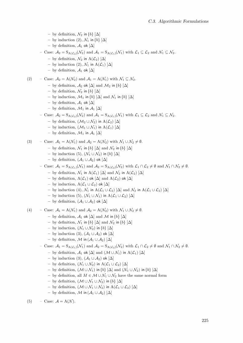
C.3. Algorithmic Formulations
– by definition, N2 in b [∆]
– by induction (2), N1 in b [∆]
– by definition, A1 ok [∆]
– Case: A2 = SA(L2)(N2) and A1 = SA(L1)(N1) with L1 ⊆ L2 and N1 ⊆ N2.
– by definition, N2 in A(L2) [∆]
– by induction (2), N1 in A(L1) [∆]
– by definition, A1 ok [∆]
(2) – Case: A2 = A(N2) and A1 = A(N1) with N1 ⊆ N2.
– by definition, A2 ok [∆] and M2 in b [∆]
– by definition, N2 in b [∆]
– by induction, M1 in b [∆] and N1 in b [∆]
– by definition, A1 ok [∆]
– by definition, M1 in A1 [∆]
– Case: A2 = SA(L2)(N2) and A1 = SA(L1)(N1) with L1 ⊆ L2 and N1 ⊆ N2.
– by definition, (M2 ∪ N2) in A(L2) [∆]
– by induction, (M1 ∪ N1) in A(L1) [∆]
– by definition, M1 in A1 [∆]
(3) – Case: A1 = A(N1) and A2 = A(N2) with N1 ∪ N2 6= ∅.
– by definition, N1 in b [∆] and N2 in b [∆]
– by induction (5), (N1 ∪ N2) in b [∆]
– by definition, (A1 ∪ A2) ok [∆]
– Case: A1 = SA(L1)(N1) and A2 = SA(L2)(N2) with L1 ∩ L2 6= ∅ and N1 ∩ N2 6= ∅.
– by definition, N1 in A(L1) [∆] and N2 in A(L2) [∆]
– by definition, A(L1) ok [∆] and A(L2) ok [∆]
– by induction, A(L1 ∪ L2) ok [∆]
– by induction (4), N1 in A(L1 ∪ L2) [∆] and N2 in A(L1 ∪ L2) [∆]
– by induction (5), (N1 ∪ N1) in A(L1 ∪ L2) [∆]
– by definition, (A1 ∪ A2) ok [∆]
(4) – Case: A1 = A(N1) and A2 = A(N2) with N1 ∪ N2 6= ∅.
– by definition, A1 ok [∆] and M in b [∆]
– by definition, N1 in b [∆] and N2 in b [∆]
– by induction, (N1 ∪ N2) in b [∆]
– by induction (3), (A1 ∪ A2) ok [∆]
– by definition, M in (A1 ∪ A2) [∆]
– Case: A1 = SA(L1)(N1) and A2 = SA(L2)(N2) with L1 ∩ L2 6= ∅ and N1 ∩ N2 6= ∅.
– by definition, A1 ok [∆] and (M∪N1) in A(L1) [∆]
– by induction (3), (A1 ∪ A2) ok [∆]
– by definition, (N1 ∪ N2) in A(L1 ∪ L2) [∆]
– by definition, (M∪N1) in b [∆] and (N1 ∪ N2) in b [∆]
– by definition, all M ∈ M∪N1 ∪ N2 have the same normal form
– by definition, (M∪N1 ∪ N2) in b [∆]
– by definition, (M∪N1 ∪ N2) in A(L1 ∪ L2) [∆]
– by definition, M in (A1 ∪ A2) [∆]
(5) – Case: A = A(N ).
225
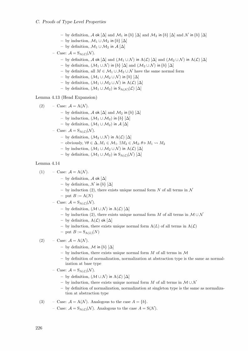
C. Proofs of Type Level Properties
– by definition, A ok [∆] and M1 in b [∆] and M2 in b [∆] and N in b [∆]
– by induction, M1 ∪M2 in b [∆]
– by definition, M1 ∪M2 in A [∆]
– Case: A = SA(L)(N ).
– by definition, A ok [∆] and (M1 ∪N ) in A(L) [∆] and (M2 ∪ N ) in A(L) [∆]
– by definition, (M1 ∪ N ) in b [∆] and (M2 ∪ N ) in b [∆]
– by definition, all M ∈ M1 ∪M2 ∪ N have the same normal form
– by definition, (M1 ∪M2 ∪ N ) in b [∆]
– by definition, (M1 ∪M2 ∪ N ) in A(L) [∆]
– by definition, (M1 ∪M2) in SA(N )(L) [∆]
Lemma 4.13 (Head Expansion)
(2) – Case: A = A(N ).
– by definition, A ok [∆] and M2 in b [∆]
– by induction, (M1 ∪M2) in b [∆]
– by definition, (M1 ∪M2) in A [∆]
– Case: A = SA(L)(N ).
– by definition, (M2 ∪ N ) in A(L) [∆]
– obviously, ∀θ ∈ ∆,M1 ∈ M1. ∃M2 ∈ M2. θ ⊲ M1 M2
– by induction, (M1 ∪M2 ∪ N ) in A(L) [∆]
– by definition, (M1 ∪M2) in SA(L)(N ) [∆]
Lemma 4.14
(1) – Case: A = A(N ).
– by definition, A ok [∆]
– by definition, N in b [∆]
– by induction (2), there exists unique normal form N of all terms in N
– put B := A(N)
– Case: A = SA(L)(N ).
– by definition, (M∪N ) in A(L) [∆]
– by induction (2), there exists unique normal form M of all terms in M∪N
– by definition, A(L) ok [∆]
– by induction, there exists unique normal form A(L) of all terms in A(L)
– put B := SA(L)(N)
(2) – Case: A = A(N ).
– by definition, M in b [∆]
– by induction, there exists unique normal form M of all terms in M
– by definition of normalization, normalization at abstraction type is the same as normal-ization at base type
– Case: A = SA(L)(N ).
– by definition, (M∪N ) in A(L) [∆]
– by induction, there exists unique normal form M of all terms in M∪N
– by definition of normalization, normalization at singleton type is the same as normaliza-tion at abstraction type
(3) – Case: A = A(N ). Analogous to the case A = b.
– Case: A = SA(L)(N ). Analogous to the case A = S(N ).
226
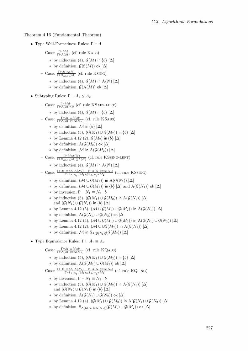
C.3. Algorithmic Formulations
Theorem 4.16 (Fundamental Theorem)
• Type Well-Formedness Rules: Γ ⊢ A
– Case: Γ⊢M :bΓ⊢A(M) (cf. rule Kabs)
∗ by induction (4), G(M) in b [∆]
∗ by definition, G(S(M)) ok [∆]
– Case: Γ⊢M :A(N)Γ⊢SA(N)(M) (cf. rule Ksing)
∗ by induction (4), G(M) in A(N) [∆]
∗ by definition, G(A(M)) ok [∆]
• Subtyping Rules: Γ ⊢ A1 ≤ A2
– Case: Γ⊢M :bΓ⊢A(M)≤b (cf. rule KSabs-left)
∗ by induction (4), G(M) in b [∆]
– Case: Γ⊢M1≡M2:bΓ⊢A(M1)≤A(M2) (cf. rule KSabs)
∗ by definition, M in b [∆]
∗ by induction (5), (G(M1) ∪ G(M2)) in b [∆]
∗ by Lemma 4.12 (2), G(M2) in b [∆]
∗ by definition, A(G(M2)) ok [∆]
∗ by definition, M in A(G(M2)) [∆]
– Case: Γ⊢M :A(N)Γ⊢SA(N)(M)≤A(N) (cf. rule KSsing-left)
∗ by induction (4), G(M) in A(N) [∆]
– Case: Γ⊢M1≡M2:A(N1) Γ⊢A(N1)≡A(N2)Γ⊢SA(N1)(M1)≤SA(N2)(M2)
(cf. rule KSsing)
∗ by definition, (M∪G(M1)) in A(G(N1)) [∆]
∗ by definition, (M∪G(M1)) in b [∆] and A(G(N1)) ok [∆]
∗ by inversion, Γ ⊢ N1 ≡ N2 : b
∗ by induction (5), (G(M1) ∪ G(M2)) in A(G(N1)) [∆]and (G(N1) ∪ G(N2)) in b [∆]
∗ by Lemma 4.12 (5), (M∪G(M1) ∪ G(M2)) in A(G(N1)) [∆]
∗ by definition, A(G(N1) ∪ G(N2)) ok [∆]
∗ by Lemma 4.12 (4), (M∪G(M1) ∪ G(M2)) in A(G(N1) ∪ G(N2)) [∆]
∗ by Lemma 4.12 (2), (M∪∪G(M2)) in A(G(N2)) [∆]
∗ by definition, M in SA(G(N2))(G(M2)) [∆]
• Type Equivalence Rules: Γ ⊢ A1 ≡ A2
– Case: Γ⊢M1≡M2:bΓ⊢A(M1)≡A(M2) (cf. rule KQabs)
∗ by induction (5), (G(M1) ∪ G(M2)) in b [∆]
∗ by definition, A(G(M1) ∪ G(M2)) ok [∆]
– Case: Γ⊢M1≡M2:A(N1) Γ⊢A(N1)≡A(N2)Γ⊢SA(N1)(M1)≡SA(N2)(M2)
(cf. rule KQsing)
∗ by inversion, Γ ⊢ N1 ≡ N2 : b
∗ by induction (5), (G(M1) ∪ G(M2)) in A(G(N1)) [∆]and (G(N1) ∪ G(N2)) in b [∆]
∗ by definition, A(G(N1) ∪ G(N2)) ok [∆]
∗ by Lemma 4.12 (4), (G(M1) ∪ G(M2)) in A(G(N1) ∪ G(N2)) [∆]
∗ by definition, SA(G(N1)∪G(N2))(G(M1) ∪ G(M2)) ok [∆]
227
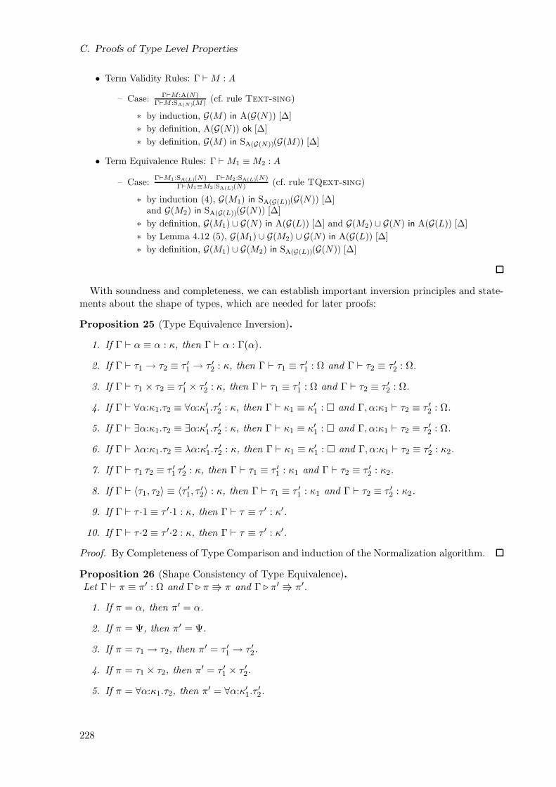
C. Proofs of Type Level Properties
• Term Validity Rules: Γ ⊢M : A
– Case: Γ⊢M :A(N)Γ⊢M :SA(N)(M) (cf. rule Text-sing)
∗ by induction, G(M) in A(G(N)) [∆]
∗ by definition, A(G(N)) ok [∆]
∗ by definition, G(M) in SA(G(N))(G(M)) [∆]
• Term Equivalence Rules: Γ ⊢M1 ≡M2 : A
– Case:Γ⊢M1:SA(L)(N) Γ⊢M2:SA(L)(N)
Γ⊢M1≡M2:SA(L)(N) (cf. rule TQext-sing)
∗ by induction (4), G(M1) in SA(G(L))(G(N)) [∆]and G(M2) in SA(G(L))(G(N)) [∆]
∗ by definition, G(M1) ∪ G(N) in A(G(L)) [∆] and G(M2) ∪ G(N) in A(G(L)) [∆]
∗ by Lemma 4.12 (5), G(M1) ∪ G(M2) ∪ G(N) in A(G(L)) [∆]
∗ by definition, G(M1) ∪ G(M2) in SA(G(L))(G(N)) [∆]
With soundness and completeness, we can establish important inversion principles and state-ments about the shape of types, which are needed for later proofs:
Proposition 25 (Type Equivalence Inversion).
1. If Γ ⊢ α ≡ α : κ, then Γ ⊢ α : Γ(α).
2. If Γ ⊢ τ1 → τ2 ≡ τ ′1 → τ ′2 : κ, then Γ ⊢ τ1 ≡ τ ′1 : Ω and Γ ⊢ τ2 ≡ τ ′2 : Ω.
3. If Γ ⊢ τ1 × τ2 ≡ τ ′1 × τ ′2 : κ, then Γ ⊢ τ1 ≡ τ ′1 : Ω and Γ ⊢ τ2 ≡ τ ′2 : Ω.
4. If Γ ⊢ ∀α:κ1.τ2 ≡ ∀α:κ′1.τ′2 : κ, then Γ ⊢ κ1 ≡ κ′1 : and Γ, α:κ1 ⊢ τ2 ≡ τ ′2 : Ω.
5. If Γ ⊢ ∃α:κ1.τ2 ≡ ∃α:κ′1.τ′2 : κ, then Γ ⊢ κ1 ≡ κ′1 : and Γ, α:κ1 ⊢ τ2 ≡ τ ′2 : Ω.
6. If Γ ⊢ λα:κ1.τ2 ≡ λα:κ′1.τ′2 : κ, then Γ ⊢ κ1 ≡ κ′1 : and Γ, α:κ1 ⊢ τ2 ≡ τ ′2 : κ2.
7. If Γ ⊢ τ1 τ2 ≡ τ ′1 τ′2 : κ, then Γ ⊢ τ1 ≡ τ ′1 : κ1 and Γ ⊢ τ2 ≡ τ ′2 : κ2.
8. If Γ ⊢ 〈τ1, τ2〉 ≡ 〈τ ′1, τ′2〉 : κ, then Γ ⊢ τ1 ≡ τ ′1 : κ1 and Γ ⊢ τ2 ≡ τ ′2 : κ2.
9. If Γ ⊢ τ ·1 ≡ τ ′·1 : κ, then Γ ⊢ τ ≡ τ ′ : κ′.
10. If Γ ⊢ τ ·2 ≡ τ ′·2 : κ, then Γ ⊢ τ ≡ τ ′ : κ′.
Proof. By Completeness of Type Comparison and induction of the Normalization algorithm.
Proposition 26 (Shape Consistency of Type Equivalence).Let Γ ⊢ π ≡ π′ : Ω and Γ ⊲ π π and Γ ⊲ π′ π′.
1. If π = α, then π′ = α.
2. If π = Ψ, then π′ = Ψ.
3. If π = τ1 → τ2, then π′ = τ ′1 → τ ′2.
4. If π = τ1 × τ2, then π′ = τ ′1 × τ ′2.
5. If π = ∀α:κ1.τ2, then π′ = ∀α:κ′1.τ′2.
228
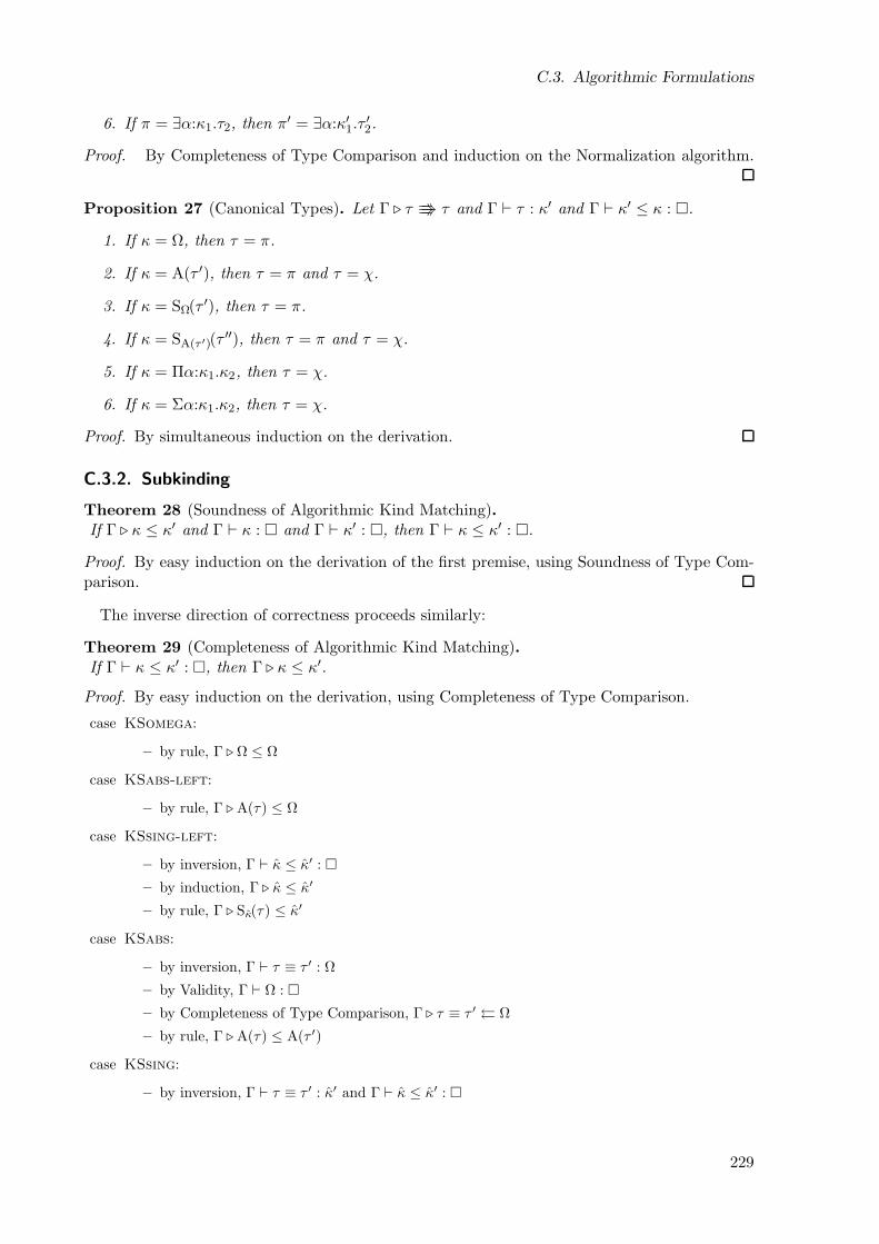
C.3. Algorithmic Formulations
6. If π = ∃α:κ1.τ2, then π′ = ∃α:κ′1.τ′2.
Proof. By Completeness of Type Comparison and induction on the Normalization algorithm.
Proposition 27 (Canonical Types). Let Γ ⊲ τ τ and Γ ⊢ τ : κ′ and Γ ⊢ κ′ ≤ κ : .
1. If κ = Ω, then τ = π.
2. If κ = A(τ ′), then τ = π and τ = χ.
3. If κ = SΩ(τ ′), then τ = π.
4. If κ = SA(τ ′)(τ′′), then τ = π and τ = χ.
5. If κ = Πα:κ1.κ2, then τ = χ.
6. If κ = Σα:κ1.κ2, then τ = χ.
Proof. By simultaneous induction on the derivation.
C.3.2. Subkinding
Theorem 28 (Soundness of Algorithmic Kind Matching).If Γ ⊲ κ ≤ κ′ and Γ ⊢ κ : and Γ ⊢ κ′ : , then Γ ⊢ κ ≤ κ′ : .
Proof. By easy induction on the derivation of the first premise, using Soundness of Type Com-parison.
The inverse direction of correctness proceeds similarly:
Theorem 29 (Completeness of Algorithmic Kind Matching).If Γ ⊢ κ ≤ κ′ : , then Γ ⊲ κ ≤ κ′.
Proof. By easy induction on the derivation, using Completeness of Type Comparison.
case KSomega:
– by rule, Γ ⊲ Ω ≤ Ω
case KSabs-left:
– by rule, Γ ⊲A(τ) ≤ Ω
case KSsing-left:
– by inversion, Γ ⊢ κ ≤ κ′ :
– by induction, Γ ⊲ κ ≤ κ′
– by rule, Γ ⊲ Sκ(τ) ≤ κ′
case KSabs:
– by inversion, Γ ⊢ τ ≡ τ ′ : Ω
– by Validity, Γ ⊢ Ω :
– by Completeness of Type Comparison, Γ ⊲ τ ≡ τ ′ Ω
– by rule, Γ ⊲A(τ) ≤ A(τ ′)
case KSsing:
– by inversion, Γ ⊢ τ ≡ τ ′ : κ′ and Γ ⊢ κ ≤ κ′ :
229
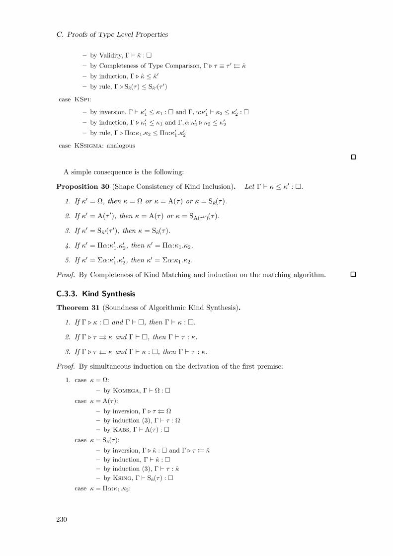
C. Proofs of Type Level Properties
– by Validity, Γ ⊢ κ :
– by Completeness of Type Comparison, Γ ⊲ τ ≡ τ ′ κ
– by induction, Γ ⊲ κ ≤ κ′
– by rule, Γ ⊲ Sκ(τ) ≤ Sκ′(τ ′)
case KSpi:
– by inversion, Γ ⊢ κ′1 ≤ κ1 : and Γ, α:κ′1 ⊢ κ2 ≤ κ′2 :
– by induction, Γ ⊲ κ′1 ≤ κ1 and Γ, α:κ′1 ⊲ κ2 ≤ κ′2
– by rule, Γ ⊲Πα:κ1.κ2 ≤ Πα:κ′1.κ′2
case KSsigma: analogous
A simple consequence is the following:
Proposition 30 (Shape Consistency of Kind Inclusion). Let Γ ⊢ κ ≤ κ′ : .
1. If κ′ = Ω, then κ = Ω or κ = A(τ) or κ = Sκ(τ).
2. If κ′ = A(τ ′), then κ = A(τ) or κ = SA(τ ′′)(τ).
3. If κ′ = Sκ′(τ ′), then κ = Sκ(τ).
4. If κ′ = Πα:κ′1.κ′2, then κ′ = Πα:κ1.κ2.
5. If κ′ = Σα:κ′1.κ′2, then κ′ = Σα:κ1.κ2.
Proof. By Completeness of Kind Matching and induction on the matching algorithm.
C.3.3. Kind Synthesis
Theorem 31 (Soundness of Algorithmic Kind Synthesis).
1. If Γ ⊲ κ : and Γ ⊢ , then Γ ⊢ κ : .
2. If Γ ⊲ τ κ and Γ ⊢ , then Γ ⊢ τ : κ.
3. If Γ ⊲ τ κ and Γ ⊢ κ : , then Γ ⊢ τ : κ.
Proof. By simultaneous induction on the derivation of the first premise:
1. case κ = Ω:
– by Komega, Γ ⊢ Ω :
case κ = A(τ):
– by inversion, Γ ⊲ τ Ω
– by induction (3), Γ ⊢ τ : Ω
– by Kabs, Γ ⊢ A(τ) :
case κ = Sκ(τ):
– by inversion, Γ ⊲ κ : and Γ ⊲ τ κ
– by induction, Γ ⊢ κ :
– by induction (3), Γ ⊢ τ : κ
– by Ksing, Γ ⊢ Sκ(τ) :
case κ = Πα:κ1.κ2:
230
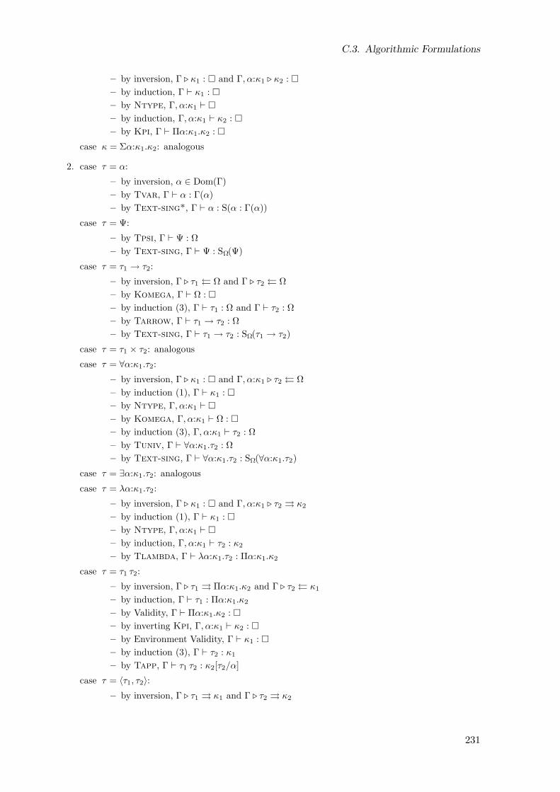
C.3. Algorithmic Formulations
– by inversion, Γ ⊲ κ1 : and Γ, α:κ1 ⊲ κ2 :
– by induction, Γ ⊢ κ1 :
– by Ntype, Γ, α:κ1 ⊢
– by induction, Γ, α:κ1 ⊢ κ2 :
– by Kpi, Γ ⊢ Πα:κ1.κ2 :
case κ = Σα:κ1.κ2: analogous
2. case τ = α:
– by inversion, α ∈ Dom(Γ)
– by Tvar, Γ ⊢ α : Γ(α)
– by Text-sing*, Γ ⊢ α : S(α : Γ(α))
case τ = Ψ:
– by Tpsi, Γ ⊢ Ψ : Ω
– by Text-sing, Γ ⊢ Ψ : SΩ(Ψ)
case τ = τ1 → τ2:
– by inversion, Γ ⊲ τ1 Ω and Γ ⊲ τ2 Ω
– by Komega, Γ ⊢ Ω :
– by induction (3), Γ ⊢ τ1 : Ω and Γ ⊢ τ2 : Ω
– by Tarrow, Γ ⊢ τ1 → τ2 : Ω
– by Text-sing, Γ ⊢ τ1 → τ2 : SΩ(τ1 → τ2)
case τ = τ1 × τ2: analogous
case τ = ∀α:κ1.τ2:
– by inversion, Γ ⊲ κ1 : and Γ, α:κ1 ⊲ τ2 Ω
– by induction (1), Γ ⊢ κ1 :
– by Ntype, Γ, α:κ1 ⊢
– by Komega, Γ, α:κ1 ⊢ Ω :
– by induction (3), Γ, α:κ1 ⊢ τ2 : Ω
– by Tuniv, Γ ⊢ ∀α:κ1.τ2 : Ω
– by Text-sing, Γ ⊢ ∀α:κ1.τ2 : SΩ(∀α:κ1.τ2)
case τ = ∃α:κ1.τ2: analogous
case τ = λα:κ1.τ2:
– by inversion, Γ ⊲ κ1 : and Γ, α:κ1 ⊲ τ2 κ2
– by induction (1), Γ ⊢ κ1 :
– by Ntype, Γ, α:κ1 ⊢
– by induction, Γ, α:κ1 ⊢ τ2 : κ2
– by Tlambda, Γ ⊢ λα:κ1.τ2 : Πα:κ1.κ2
case τ = τ1 τ2:
– by inversion, Γ ⊲ τ1 Πα:κ1.κ2 and Γ ⊲ τ2 κ1
– by induction, Γ ⊢ τ1 : Πα:κ1.κ2
– by Validity, Γ ⊢ Πα:κ1.κ2 :
– by inverting Kpi, Γ, α:κ1 ⊢ κ2 :
– by Environment Validity, Γ ⊢ κ1 :
– by induction (3), Γ ⊢ τ2 : κ1
– by Tapp, Γ ⊢ τ1 τ2 : κ2[τ2/α]
case τ = 〈τ1, τ2〉:
– by inversion, Γ ⊲ τ1 κ1 and Γ ⊲ τ2 κ2
231
C. Proofs of Type Level Properties
– by induction, Γ ⊢ τ1 : κ1 and Γ ⊢ τ2 : κ2
– by Validity, Γ ⊢ κ1 : and Γ ⊢ κ2 :
– w.l.o.g., α /∈ Dom(Γ)
– by Ntype, Γ, α:κ1 ⊢
– by Weakening, Γ, α:κ1 ⊢ κ2 :
– by Ksigma, Γ ⊢ Σα:κ1.κ2 :
– by Tpair, Γ ⊢ 〈τ1, τ2〉 : Σα:κ1.κ2
case τ = τ ·1:
– by inversion, Γ ⊲ τ Σα:κ1.κ2
– by induction, Γ ⊢ τ : Σα:κ1.κ2
– by Tfst, Γ ⊢ τ ·1 : κ1
case τ = τ ·2: analogous
3. case Γ ⊲ τ κ:
– by inversion, Γ ⊲ τ κ′ and Γ ⊲ κ′ ≤ κ
– by Environment Validity, Γ ⊢
– by induction (2), Γ ⊢ τ : κ′
– by Validity, Γ ⊢ κ′ :
– by Soundness of Kind Matching, Γ ⊢ κ′ ≤ κ :
– by Tsub, Γ ⊢ τ : κ
Theorem 32 (Completeness of Algorithmic Kind Synthesis).
1. If Γ ⊢ κ : , then Γ ⊲ κ : .
2. If Γ ⊢ τ : κ, then Γ ⊲ τ κ′ and Γ ⊢ κ′ ≤ S(τ : κ) : .
3. If Γ ⊢ τ : κ, then Γ ⊲ τ κ.
Proof. By simultaneous induction on the derivation:
1. case Komega: directly
case Kabs:
– by inversion, Γ ⊢ τ : Ω
– by induction (3), Γ ⊲ τ Ω
– by rule, Γ ⊲A(τ) :
case Ksing:
– by inversion, Γ ⊢ τ : κ
– by Validity, Γ ⊢ κ :
– by induction, Γ ⊲ κ :
– by induction (3), Γ ⊲ τ κ
– by rule, Γ ⊲ Sκ(τ) :
case Kpi:
– by inversion, Γ, α:κ1 ⊢ κ2 :
– by Environment Validity, Γ ⊢ κ1 :
– by induction, Γ ⊲ κ1 : and Γ, α:κ1 ⊲ κ2 :
– by rule, Γ ⊲Πα:κ1.κ2 :
case Ksigma: analogous
232
C.3. Algorithmic Formulations
2. case Tvar:
– by inversion, κ = Γ(α)
– by rule, Γ ⊲ α S(α : Γ(α))
– by Reflexivity, Γ ⊢ α ≡ α : Γ(α)
– by Validity, Γ ⊢ Γ(α) :
– by Reflexivity, Γ ⊢ Γ(α) ≤ Γ(α) :
– by KSsing*, Γ ⊢ S(α : Γ(α)) ≤ S(α : Γ(α)) :
case Tpsi:
– by rule, Γ ⊲Ψ SΩ(Ψ)
– by Text-sing, Γ ⊢ SΩ(Ψ) :
– by Reflexivity, Γ ⊢ SΩ(Ψ) ≤ SΩ(Ψ) :
case Tarrow:
– by inversion, Γ ⊢ τ1 : Ω and Γ ⊢ τ1 : Ω
– by induction (3), Γ ⊲ τ1 Ω and Γ ⊲ τ1 Ω
– by rule, Γ ⊲ τ1 → τ2 SΩ(τ1 → τ2)
– by Text-sing, Γ ⊢ SΩ(τ1 → τ2) :
– by Reflexivity, Γ ⊢ SΩ(τ1 → τ2) ≤ SΩ(τ1 → τ2) :
case Ttimes: analogous
case Tuniv:
– by inversion, Γ, α:κ1 ⊢ τ2 : Ω
– by Environment Validity, Γ ⊢ κ1 :
– by induction (1), Γ ⊲ κ1 :
– by induction (3), Γ, α:κ1 ⊲ τ2 Ω
– by rule, Γ ⊲ ∀α:κ1.τ2 SΩ(∀α:κ1.τ2)
– by Text-sing, Γ ⊢ SΩ(∀α:κ1.τ2) :
– by Reflexivity, Γ ⊢ SΩ(∀α:κ1.τ2) ≤ SΩ(∀α:κ1.τ2) :
case Texist: analogous
case Tlambda:
– by inversion, Γ, α:κ1 ⊢ τ2 : κ2
– by Environment Validity, Γ ⊢ κ1 :
– by induction (1), Γ ⊲ κ1 :
– by induction, Γ, α:κ1 ⊲ τ2 κ′2 and Γ, α:κ1 ⊢ κ′2 ≤ S(τ2 : κ2) :
– by rule, Γ ⊲ λα:κ1.τ2 Πα:κ1.κ′2
– by Reflexivity, Γ ⊢ κ1 ≤ κ1 :
– by Validity, Γ, α:κ1 ⊢ κ′2 :
– by Kpi, Γ ⊢ Πα:κ1.κ′2 :
– by KSpi, Γ ⊢ Πα:κ1.κ′2 ≤ Πα:κ1.S(τ2 : κ2) :
case Tapp:
– by inversion, Γ ⊢ τ1 : Πα:κ1.κ2 and Γ ⊢ τ2 : κ1 and κ = κ2[τ2/α]
– by induction, Γ ⊲ τ1 κ′ and Γ ⊢ κ′ ≤ Πα:κ1.S(τ1 α : κ2) :
– by Kind Inclusion Inversion, κ′ = Πα:κ′1.κ′2 and Γ ⊢ κ1 ≤ κ′1 :
and Γ, α:κ1 ⊢ κ′2 ≤ S(τ1 α : κ2) :
– by Tsub, Γ ⊢ τ2 : κ′1– by induction (3), Γ ⊲ τ2 κ′1– by rule, Γ ⊲ τ1 τ2 κ′2[τ2/α]
– by Environment Validity, Γ, α:κ1 ⊢
233
C. Proofs of Type Level Properties
– obviously, Γ ⊢ [τ2/α] : Γ, α:κ1
– by Substitutability, Γ ⊢ κ′2[τ2/α] ≤ S(τ1 α : κ2)[τ2/α] :
– by Tvar, Γ, α:κ1 ⊢ α : κ1
– by Weakening, Γ, α:κ1 ⊢ τ1 : Πα:κ1.κ2
– by Tapp, Γ, α:κ1 ⊢ τ1 α : κ2
– by KSsing-left*, Γ, α:κ1 ⊢ S(τ1 α : κ2) ≤ κ2 :
– by Substitutability, Γ ⊢ S(τ1 α : κ2)[τ2/α] ≤ κ2[τ2/α] :
– by Transitivity, Γ ⊢ κ′2[τ2/α] ≤ κ2[τ2/α] :
case Tpair:
– by inversion, Γ ⊢ τ1 : κ1 and Γ ⊢ τ2 : κ2[τ1/α]
– by induction, Γ ⊲ τ1 κ′1 and Γ ⊢ κ′1 ≤ S(τ1 : κ1) : and Γ ⊲ τ2 κ′2 and Γ ⊢ κ′2 ≤ S(τ2 : κ2[τ1/α]) :
– by rule, Γ ⊲ 〈τ1, τ2〉 κ′1 × κ′2– by Validity, Γ ⊢ κ′1 :
– w.l.o.g., α /∈ Dom(Γ) ∪ FV(τ)
– by Ntype, Γ, α:κ′1 ⊢
– by Weakening, Γ, α:κ′1 ⊢ κ′2 ≤ S(τ2 : κ2[τ1/α]) :
– by Validity and Ksigma, Γ ⊢ S(τ1 : κ1) × S(τ2 : κ2[τ1/α]) :
– by KSsigma, Γ ⊢ κ′1 × κ′2 ≤ S(τ1 : κ1) × S(τ2 : κ2[τ1/α]) :
case Tfst:
– by inversion, Γ ⊢ τ : Σα:κ1.κ2
– by induction, Γ ⊲ τ κ and Γ ⊢ κ ≤ S(τ ·1 : κ1) × S(τ ·2 : κ2[τ ·1/α]) :
– by Kind Inclusion Inversion, κ = Σα:κ′1.κ′2 and Γ ⊢ κ′1 ≤ S(τ ·1 : κ1) :
– by rule, Γ ⊲ τ ·1 κ′1
case Tsnd: similarly
case Text-sing:
– by inversion, Γ ⊢ τ : κ
– by induction, Γ ⊲ τ κ and Γ ⊢ κ ≤ Sκ(τ) :
case Text-pi:
– by inversion, Γ ⊢ τ : Πα:κ1.κ′2 and Γ, α:κ1 ⊢ τ α : κ2
– by induction, Γ ⊲ τ κ and Γ ⊢ κ ≤ Πα:κ1.S(τ α : κ′2) : and Γ, α:κ1 ⊲ τ α κ′′2 and Γ, α:κ1 ⊢ κ′′2 ≤ S(τ α : κ2) :
– by inverting Γ, α:κ1 ⊲ τ α κ′′2 , we know that κ = Πα:κ′1.κ′′2
– by inverting KSpi, Γ ⊢ κ1 ≤ κ′1 :
– by KSpi, Γ ⊢ κ ≤ Πα:κ1.S(τ α : κ2) :
case Text-sigma:
– by inversion, Γ ⊢ τ ·1 : κ1 and Γ ⊢ τ ·2 : κ2[τ ·1/α]
– by induction, Γ ⊲ τ ·1 κ′1 and Γ ⊢ κ′1 ≤ S(τ ·1 : κ1) : and Γ ⊲ τ ·2 κ′2 and Γ ⊢ κ′2 ≤ S(τ ·2 : κ2)[τ ·1/α] :
– by inverting Γ ⊲ τ ·1 κ′1, we know that Γ ⊲ τ Σα:κ′1.κ′′2
– by inverting Γ ⊲ τ ·2 κ′2, we further know that κ′2 = κ′′2 [τ ·1/α]
– by Validity, Γ ⊢ κ′1 :
– w.l.o.g., α /∈ Dom(Γ) ∪ FV(τ)
– by Ntype, Γ, α:κ′1 ⊢
– by Weakening, Γ, α:κ′1 ⊢ κ′2 ≤ S(τ ·2 : κ2)[τ ·1/α] :
– by Validity and Ksigma, Γ ⊢ S(τ ·1 : κ1) × S(τ ·2 : κ2[τ ·1/α]) :
– by KSsigma, Γ ⊢ Σα:κ′1.κ′′2 ≤ S(τ ·1 : κ1) × S(τ ·2 : κ2[τ ·1/α]) :
234
C.3. Algorithmic Formulations
case Tsub:
– by inversion, Γ ⊢ τ : κ′ and Γ ⊢ κ′ ≤ κ :
– by induction, Γ ⊲ τ κ′′ and Γ ⊢ κ′′ ≤ S(τ : κ′) :
– by Reflexivity, Γ ⊢ τ ≡ τ : κ′
– by KSsing*, Γ ⊢ S(τ : κ′) ≤ S(τ : κ) :
– by Transitivity, Γ ⊢ κ′′ ≤ S(τ : κ) :
3. • by induction (2), Γ ⊲ τ κ′ and Γ ⊢ κ′ ≤ S(τ : κ) :
• by KSsing-left, Γ ⊢ S(τ : κ) ≤ κ :
• by Transitivity, Γ ⊢ κ′ ≤ κ :
• by Completeness of Kind Matching, Γ ⊲ κ′ ≤ κ
• by rule, Γ ⊲ τ κ
C.3.4. Subtyping
Theorem 33 (Soundness of Algorithmic Type Matching).
1. If Γ ⊲ τ ≤ τ ′ κ and Γ ⊢ τ : κ and Γ ⊢ τ ′ : κ, then Γ ⊢ τ ≤ τ ′ : κ.
2. If Γ ⊲ π ⊑ π′ and Γ ⊢ π : Ω and Γ ⊢ π′ : Ω, then Γ ⊢ π ≤ π′ : Ω.
Proof. By simultaneous induction on the derivation:
1. case κ = Ω:
– bz inversion, Γ ⊲ τ π Ω and Γ ⊲ τ ′ π′ Ω and Γ ⊲ π ⊑ π′
– by Soundness of Type Comparison, Γ ⊢ τ ≡ π : Ω and Γ ⊢ τ ′ ≡ π′ : Ω
– by Validity, Γ ⊢ π : Ω and Γ ⊢ π′ : Ω
– by induction (2), Γ ⊢ π ≤ π′ : Ω
– by Symmetry, TSequiv, and Transitivity, Γ ⊢ τ ≤ τ ′ : Ω
case κ 6= Ω:
– by inversion, Γ ⊲ τ ≡ τ ′ κ
– by Soundness of Type Comparison, Γ ⊢ τ ≡ τ ′ : κ
2. case π = χ and π′ = χ′:
– bz inversion, Γ ⊲ χ ≡ χ′ Ω
– by Soundness of Type Comparison, Γ ⊢ χ ≡ χ′ : Ω
case π = τ1 → τ2 and π′ = τ ′1 → τ ′2:
– by inversion, Γ ⊲ τ ′1 ≤ τ1 Ω and Γ ⊲ τ2 ≤ τ ′2 Ω
– by Type Validity Inversion, Γ ⊢ τ1 : Ω and Γ ⊢ τ2 : Ω and Γ ⊢ τ ′1 : Ω and Γ ⊢ τ ′2 : Ω
– by induction (1), Γ ⊢ τ ′1 ≤ τ1 : Ω and Γ ⊢ τ2 ≤ τ ′2 : Ω
– by TSarrow, Γ ⊢ τ1 → τ2 ≤ τ ′1 → τ ′2 : Ω
case π = τ1 × τ2 and π′ = τ ′1 × τ ′2: analogous
case π = ∀α:κ.τ and π′ = ∀α:κ′.τ ′:
– by inversion, Γ ⊲ κ′ ≤ κ and Γ, α:κ′ ⊲ τ ≤ τ ′ Ω
– by Type Validity Inversion, Γ, α:κ ⊢ τ : Ω and Γ, α:κ′ ⊢ τ ′ : Ω
– by Environment Validity, Γ ⊢ κ : and Γ ⊢ κ′ :
– by Soundness of Kind Matching, Γ ⊢ κ′ ≤ κ :
– by Weakening, Γ, α:κ′ ⊢ τ : Ω
235
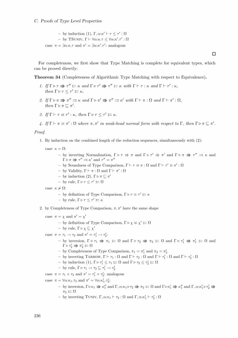
C. Proofs of Type Level Properties
– by induction (1), Γ, α:κ′ ⊢ τ ≤ τ ′ : Ω
– by TSuniv, Γ ⊢ ∀α:κ.τ ≤ ∀α:κ′.τ ′ : Ω
case π = ∃α:κ.τ and π′ = ∃α:κ′.τ ′: analogous
For completeness, we first show that Type Matching is complete for equivalent types, whichcan be proved directly:
Theorem 34 (Completeness of Algorithmic Type Matching with respect to Equivalence).
1. If Γ ⊲ τ τ ′′ κ and Γ ⊲ τ ′ τ ′′ κ with Γ ⊢ τ : κ and Γ ⊢ τ ′ : κ,then Γ ⊲ τ ≤ τ ′ κ.
2. If Γ ⊲ π π′′ κ and Γ ⊲ π′ π′′ κ′ with Γ ⊢ π : Ω and Γ ⊢ π′ : Ω,then Γ ⊲ π ⊑ π′.
3. If Γ ⊢ τ ≡ τ ′ : κ, then Γ ⊲ τ ≤ τ ′ κ.
4. If Γ ⊢ π ≡ π′ : Ω where π, π′ in weak-head normal form with respect to Γ, then Γ ⊲ π ⊑ π′.
Proof.
1. By induction on the combined length of the reduction sequences, simultaneously with (2):
case κ = Ω:
– by inverting Normalization, Γ ⊲ τ π and Γ ⊲ τ ′ π′ and Γ ⊲ π τ ′′ κ andΓ ⊲ π τ ′′ κ′ and τ ′′ = π′′
– by Soundness of Type Comparison, Γ ⊢ τ ≡ π : Ω and Γ ⊢ τ ′ ≡ π′ : Ω
– by Validity, Γ ⊢ π : Ω and Γ ⊢ π′ : Ω
– by induction (2), Γ ⊲ π ⊑ π′
– by rule, Γ ⊲ τ ≤ τ ′ Ω
case κ 6= Ω:
– by definition of Type Comparison, Γ ⊲ τ ≡ τ ′ κ
– by rule, Γ ⊲ τ ≤ τ ′ κ
2. by Completeness of Type Comparison, π, π′ have the same shape
case π = χ and π′ = χ′
– by definition of Type Comparison, Γ ⊲ χ ≡ χ′ Ω
– by rule, Γ ⊲ χ ⊑ χ′
case π = τ1 → τ2 and π′ = τ ′1 → τ ′2:
– by inversion, Γ ⊲ τ1 π1 Ω and Γ ⊲ τ2 π2 Ω and Γ ⊲ τ ′1 π′1 Ω and
Γ ⊲ τ ′2 π′2 Ω
– by Completeness of Type Comparison, π1 = π′1 and π2 = π′
2
– by inverting Tarrow, Γ ⊢ τ1 : Ω and Γ ⊢ τ2 : Ω and Γ ⊢ τ ′1 : Ω and Γ ⊢ τ ′2 : Ω
– by induction (1), Γ ⊲ τ ′1 ≤ τ1 Ω and Γ ⊲ τ2 ≤ τ ′2 Ω
– by rule, Γ ⊲ τ1 → τ2 ⊑ τ ′1 → τ ′2
case π = τ1 × τ2 and π′ = τ ′1 × τ ′2: analogous
case π = ∀α:κ1.τ2 and π′ = ∀α:κ′1.τ′2:
– by inversion, Γ⊲κ1 κ′′1 and Γ, α:κ1 ⊲τ2 π2 Ω and Γ⊲κ′1 κ′′1 and Γ, α:κ′1 ⊲τ′2
π2 Ω
– by inverting Tuniv, Γ, α:κ1 ⊢ τ2 : Ω and Γ, α:κ′1 ⊢ τ ′2 : Ω
236
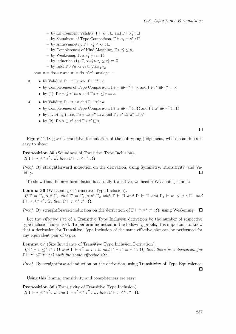
C.3. Algorithmic Formulations
– by Environment Validity, Γ ⊢ κ1 : and Γ ⊢ κ′1 :
– by Soundness of Type Comparison, Γ ⊢ κ1 ≡ κ′1 :
– by Antisymmetry, Γ ⊢ κ′1 ≤ κ1 :
– by Completeness of Kind Matching, Γ ⊲ κ′1 ≤ κ1
– by Weakening, Γ, α:κ′1 ⊢ τ2 : Ω
– by induction (1), Γ, α:κ′1 ⊲ τ2 ≤ τ ′2 Ω
– by rule, Γ ⊲ ∀α:κ1.τ2 ⊑ ∀α:κ′1.τ′2
case π = ∃α:κ.τ and π′ = ∃α:κ′.τ ′: analogous
3. • by Validity, Γ ⊢ τ : κ and Γ ⊢ τ ′ : κ
• by Completeness of Type Comparison, Γ ⊲ τ τ ′′ κ and Γ ⊲ τ ′ τ ′′ κ
• by (1), Γ ⊲ τ ≤ τ ′ κ and Γ ⊲ τ ′ ≤ τ κ
4. • by Validity, Γ ⊢ π : κ and Γ ⊢ π′ : κ
• by Completeness of Type Comparison, Γ ⊲ π π′′ Ω and Γ ⊲ π′ π′′ Ω
• by inverting these, Γ ⊲ π π′′ κ and Γ ⊲ π′ π′′ κ′
• by (2), Γ ⊲ π ⊑ π′ and Γ ⊲ π′ ⊑ π
Figure 11.18 gave a transitive formulation of the subtyping judgement, whose soundness iseasy to show:
Proposition 35 (Soundness of Transitive Type Inclusion).If Γ ⊢ τ ≤∗ τ ′ : Ω, then Γ ⊢ τ ≤ τ ′ : Ω.
Proof. By straightforward induction on the derivation, using Symmetry, Transitivity, and Va-lidity.
To show that the new formulation is actually transitive, we need a Weakening lemma:
Lemma 36 (Weakening of Transitive Type Inclusion).If Γ = Γ1, α:κ,Γ2 and Γ′ = Γ1, α:κ′,Γ2 with Γ ⊢ and Γ′ ⊢ and Γ1 ⊢ κ′ ≤ κ : , and
Γ ⊢ τ ≤∗ τ ′ : Ω, then Γ ⊢ τ ≤∗ τ ′ : Ω.
Proof. By straightforward induction on the derivation of Γ ⊢ τ ≤∗ τ ′ : Ω, using Weakening.
Let the effective size of a Transitive Type Inclusion derivation be the number of respectivetype inclusion rules used. To perform induction in the following proofs, it is important to knowthat a derivation for Transitive Type Inclusion of the same effective size can be performed forany equivalent pair of types:
Lemma 37 (Size Invariance of Transitive Type Inclusion Derivation).If Γ ⊢ τ ≤∗ τ ′ : Ω and Γ ⊢ τ ′′ ≡ τ : Ω and Γ ⊢ τ ′ ≡ τ ′′′ : Ω, then there is a derivation for
Γ ⊢ τ ′′ ≤∗ τ ′′′ : Ω with the same effective size.
Proof. By straightforward induction on the derivation, using Transitivity of Type Equivalence.
Using this lemma, transitivity and completeness are easy:
Proposition 38 (Transitivity of Transitive Type Inclusion).If Γ ⊢ τ ≤∗ τ ′ : Ω and Γ ⊢ τ ′ ≤∗ τ ′′ : Ω, then Γ ⊢ τ ≤∗ τ ′′ : Ω.
237
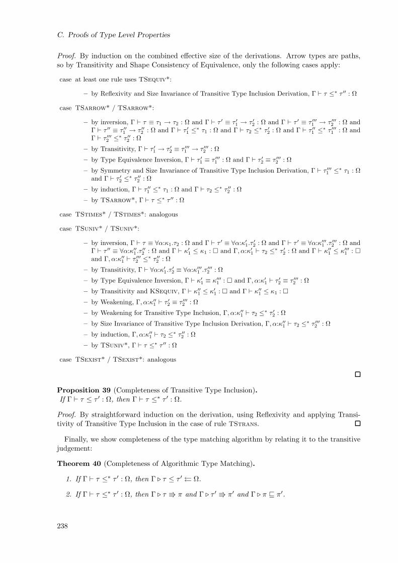
C. Proofs of Type Level Properties
Proof. By induction on the combined effective size of the derivations. Arrow types are paths,so by Transitivity and Shape Consistency of Equivalence, only the following cases apply:
case at least one rule uses TSequiv*:
– by Reflexivity and Size Invariance of Transitive Type Inclusion Derivation, Γ ⊢ τ ≤∗ τ ′′ : Ω
case TSarrow* / TSarrow*:
– by inversion, Γ ⊢ τ ≡ τ1 → τ2 : Ω and Γ ⊢ τ ′ ≡ τ ′1 → τ ′2 : Ω and Γ ⊢ τ ′ ≡ τ ′′′1 → τ ′′′2 : Ω andΓ ⊢ τ ′′ ≡ τ ′′1 → τ ′′2 : Ω and Γ ⊢ τ ′1 ≤∗ τ1 : Ω and Γ ⊢ τ2 ≤∗ τ ′2 : Ω and Γ ⊢ τ ′′1 ≤∗ τ ′′′1 : Ω andΓ ⊢ τ ′′′2 ≤∗ τ ′′2 : Ω
– by Transitivity, Γ ⊢ τ ′1 → τ ′2 ≡ τ ′′′1 → τ ′′′2 : Ω
– by Type Equivalence Inversion, Γ ⊢ τ ′1 ≡ τ ′′′1 : Ω and Γ ⊢ τ ′2 ≡ τ ′′′2 : Ω
– by Symmetry and Size Invariance of Transitive Type Inclusion Derivation, Γ ⊢ τ ′′′1 ≤∗ τ1 : Ωand Γ ⊢ τ ′2 ≤∗ τ ′′2 : Ω
– by induction, Γ ⊢ τ ′′1 ≤∗ τ1 : Ω and Γ ⊢ τ2 ≤∗ τ ′′2 : Ω
– by TSarrow*, Γ ⊢ τ ≤∗ τ ′′ : Ω
case TStimes* / TStimes*: analogous
case TSuniv* / TSuniv*:
– by inversion, Γ ⊢ τ ≡ ∀α:κ1.τ2 : Ω and Γ ⊢ τ ′ ≡ ∀α:κ′1.τ′2 : Ω and Γ ⊢ τ ′ ≡ ∀α:κ′′′1 .τ
′′′2 : Ω and
Γ ⊢ τ ′′ ≡ ∀α:κ′′1 .τ′′2 : Ω and Γ ⊢ κ′1 ≤ κ1 : and Γ, α:κ′1 ⊢ τ2 ≤∗ τ ′2 : Ω and Γ ⊢ κ′′1 ≤ κ′′′1 :
and Γ, α:κ′′1 ⊢ τ ′′′2 ≤∗ τ ′′2 : Ω
– by Transitivity, Γ ⊢ ∀α:κ′1.τ′2 ≡ ∀α:κ′′′1 .τ
′′′2 : Ω
– by Type Equivalence Inversion, Γ ⊢ κ′1 ≡ κ′′′1 : and Γ, α:κ′1 ⊢ τ ′2 ≡ τ ′′′2 : Ω
– by Transitivity and KSequiv, Γ ⊢ κ′′1 ≤ κ′1 : and Γ ⊢ κ′′1 ≤ κ1 :
– by Weakening, Γ, α:κ′′1 ⊢ τ ′2 ≡ τ ′′′2 : Ω
– by Weakening for Transitive Type Inclusion, Γ, α:κ′′1 ⊢ τ2 ≤∗ τ ′2 : Ω
– by Size Invariance of Transitive Type Inclusion Derivation, Γ, α:κ′′1 ⊢ τ2 ≤∗ τ ′′′2 : Ω
– by induction, Γ, α:κ′′1 ⊢ τ2 ≤∗ τ ′′2 : Ω
– by TSuniv*, Γ ⊢ τ ≤∗ τ ′′ : Ω
case TSexist* / TSexist*: analogous
Proposition 39 (Completeness of Transitive Type Inclusion).If Γ ⊢ τ ≤ τ ′ : Ω, then Γ ⊢ τ ≤∗ τ ′ : Ω.
Proof. By straightforward induction on the derivation, using Reflexivity and applying Transi-tivity of Transitive Type Inclusion in the case of rule TStrans.
Finally, we show completeness of the type matching algorithm by relating it to the transitivejudgement:
Theorem 40 (Completeness of Algorithmic Type Matching).
1. If Γ ⊢ τ ≤∗ τ ′ : Ω, then Γ ⊲ τ ≤ τ ′ Ω.
2. If Γ ⊢ τ ≤∗ τ ′ : Ω, then Γ ⊲ τ π and Γ ⊲ τ ′ π′ and Γ ⊲ π ⊑ π′.
238
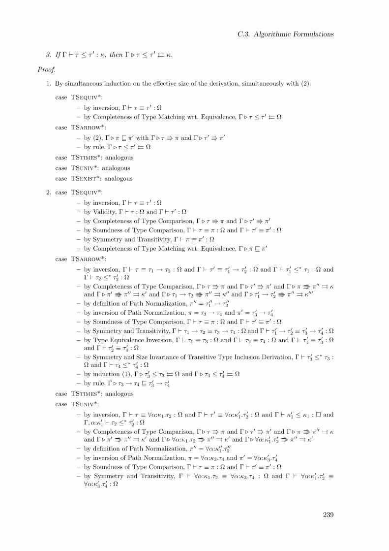
C.3. Algorithmic Formulations
3. If Γ ⊢ τ ≤ τ ′ : κ, then Γ ⊲ τ ≤ τ ′ κ.
Proof.
1. By simultaneous induction on the effective size of the derivation, simultaneously with (2):
case TSequiv*:
– by inversion, Γ ⊢ τ ≡ τ ′ : Ω
– by Completeness of Type Matching wrt. Equivalence, Γ ⊲ τ ≤ τ ′ Ω
case TSarrow*:
– by (2), Γ ⊲ π ⊑ π′ with Γ ⊲ τ π and Γ ⊲ τ ′ π′
– by rule, Γ ⊲ τ ≤ τ ′ Ω
case TStimes*: analogous
case TSuniv*: analogous
case TSexist*: analogous
2. case TSequiv*:
– by inversion, Γ ⊢ τ ≡ τ ′ : Ω
– by Validity, Γ ⊢ τ : Ω and Γ ⊢ τ ′ : Ω
– by Completeness of Type Comparison, Γ ⊲ τ π and Γ ⊲ τ ′ π′
– by Soundness of Type Comparison, Γ ⊢ τ ≡ π : Ω and Γ ⊢ τ ′ ≡ π′ : Ω
– by Symmetry and Transitivity, Γ ⊢ π ≡ π′ : Ω
– by Completeness of Type Matching wrt. Equivalence, Γ ⊲ π ⊑ π′
case TSarrow*:
– by inversion, Γ ⊢ τ ≡ τ1 → τ2 : Ω and Γ ⊢ τ ′ ≡ τ ′1 → τ ′2 : Ω and Γ ⊢ τ ′1 ≤∗ τ1 : Ω andΓ ⊢ τ2 ≤∗ τ ′2 : Ω
– by Completeness of Type Comparison, Γ ⊲ τ π and Γ ⊲ τ ′ π′ and Γ ⊲ π π′′ κand Γ ⊲ π′ π′′ κ′ and Γ ⊲ τ1 → τ2 π′′ κ′′ and Γ ⊲ τ ′1 → τ ′2 π′′ κ′′′
– by definition of Path Normalization, π′′ = τ ′′1 → τ ′′2– by inversion of Path Normalization, π = τ3 → τ4 and π′ = τ ′3 → τ ′4– by Soundness of Type Comparison, Γ ⊢ τ ≡ π : Ω and Γ ⊢ τ ′ ≡ π′ : Ω
– by Symmetry and Transitivity, Γ ⊢ τ1 → τ2 ≡ τ3 → τ4 : Ω and Γ ⊢ τ ′1 → τ ′2 ≡ τ ′3 → τ ′4 : Ω
– by Type Equivalence Inversion, Γ ⊢ τ1 ≡ τ3 : Ω and Γ ⊢ τ2 ≡ τ4 : Ω and Γ ⊢ τ ′1 ≡ τ ′3 : Ωand Γ ⊢ τ ′2 ≡ τ ′4 : Ω
– by Symmetry and Size Invariance of Transitive Type Inclusion Derivation, Γ ⊢ τ ′3 ≤∗ τ3 :Ω and Γ ⊢ τ4 ≤∗ τ ′4 : Ω
– by induction (1), Γ ⊲ τ ′3 ≤ τ3 Ω and Γ ⊲ τ4 ≤ τ ′4 Ω
– by rule, Γ ⊲ τ3 → τ4 ⊑ τ ′3 → τ ′4
case TStimes*: analogous
case TSuniv*:
– by inversion, Γ ⊢ τ ≡ ∀α:κ1.τ2 : Ω and Γ ⊢ τ ′ ≡ ∀α:κ′1.τ′2 : Ω and Γ ⊢ κ′1 ≤ κ1 : and
Γ, α:κ′1 ⊢ τ2 ≤∗ τ ′2 : Ω
– by Completeness of Type Comparison, Γ ⊲ τ π and Γ ⊲ τ ′ π′ and Γ ⊲ π π′′ κand Γ ⊲ π′ π′′ κ′ and Γ ⊲ ∀α:κ1.τ2 π′′ κ′ and Γ ⊲ ∀α:κ′1.τ
′2 π′′ κ′
– by definition of Path Normalization, π′′ = ∀α:κ′′1 .τ′′2
– by inversion of Path Normalization, π = ∀α:κ3.τ4 and π′ = ∀α:κ′3.τ′4
– by Soundness of Type Comparison, Γ ⊢ τ ≡ π : Ω and Γ ⊢ τ ′ ≡ π′ : Ω
– by Symmetry and Transitivity, Γ ⊢ ∀α:κ1.τ2 ≡ ∀α:κ3.τ4 : Ω and Γ ⊢ ∀α:κ′1.τ′2 ≡
∀α:κ′3.τ′4 : Ω
239
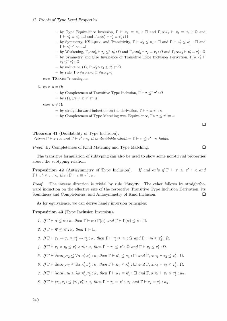
C. Proofs of Type Level Properties
– by Type Equivalence Inversion, Γ ⊢ κ1 ≡ κ3 : and Γ, α:κ1 ⊢ τ2 ≡ τ4 : Ω andΓ ⊢ κ′1 ≡ κ′3 : and Γ, α:κ′1 ⊢ τ ′2 ≡ τ ′4 : Ω
– by Symmetry, KSequiv, and Transitivity, Γ ⊢ κ′3 ≤ κ1 : and Γ ⊢ κ′3 ≤ κ′1 : andΓ ⊢ κ′3 ≤ κ3 :
– by Weakening, Γ, α:κ′3 ⊢ τ2 ≤∗ τ ′2 : Ω and Γ, α:κ′3 ⊢ τ2 ≡ τ4 : Ω and Γ, α:κ′3 ⊢ τ ′2 ≡ τ ′4 : Ω
– by Symmetry and Size Invariance of Transitive Type Inclusion Derivation, Γ, α:κ′3 ⊢τ4 ≤∗ τ ′4 : Ω
– by induction (1), Γ, κ′3 ⊲ τ4 ≤ τ ′4 Ω
– by rule, Γ ⊲ ∀α:κ3.τ4 ⊑ ∀α:κ′3.τ′4
case TSexist*: analogous
3. case κ = Ω:
– by Completeness of Transitive Type Inclusion, Γ ⊢ τ ≤∗ τ ′ : Ω
– by (1), Γ ⊲ τ ≤ τ ′ Ω
case κ 6= Ω:
– by straightforward induction on the derivation, Γ ⊢ τ ≡ τ ′ : κ
– by Completeness of Type Matching wrt. Equivalence, Γ ⊲ τ ≤ τ ′ κ
Theorem 41 (Decidability of Type Inclusion).Given Γ ⊢ τ : κ and Γ ⊢ τ ′ : κ, it is decidable whether Γ ⊢ τ ≤ τ ′ : κ holds.
Proof. By Completeness of Kind Matching and Type Matching.
The transitive formulation of subtyping can also be used to show some non-trivial propertiesabout the subtyping relation:
Proposition 42 (Antisymmetry of Type Inclusion). If and only if Γ ⊢ τ ≤ τ ′ : κ andΓ ⊢ τ ′ ≤ τ : κ, then Γ ⊢ τ ≡ τ ′ : κ.
Proof. The inverse direction is trivial by rule TSequiv. The other follows by straightfor-ward induction on the effective size of the respective Transitive Type Inclusion Derivation, itsSoundness and Completeness, and Antisymmetry of Kind Inclusion.
As for equivalence, we can derive handy inversion principles:
Proposition 43 (Type Inclusion Inversion).
1. If Γ ⊢ α ≤ α : κ, then Γ ⊢ α : Γ(α) and Γ ⊢ Γ(α) ≤ κ : .
2. If Γ ⊢ Ψ ≤ Ψ : κ, then Γ ⊢ .
3. If Γ ⊢ τ1 → τ2 ≤ τ ′1 → τ ′2 : κ, then Γ ⊢ τ ′1 ≤ τ1 : Ω and Γ ⊢ τ2 ≤ τ ′2 : Ω.
4. If Γ ⊢ τ1 × τ2 ≤ τ ′1 × τ ′2 : κ, then Γ ⊢ τ1 ≤ τ ′1 : Ω and Γ ⊢ τ2 ≤ τ ′2 : Ω.
5. If Γ ⊢ ∀α:κ1.τ2 ≤ ∀α:κ′1.τ′2 : κ, then Γ ⊢ κ′1 ≤ κ1 : and Γ, α:κ1 ⊢ τ2 ≤ τ ′2 : Ω.
6. If Γ ⊢ ∃α:κ1.τ2 ≤ ∃α:κ′1.τ′2 : κ, then Γ ⊢ κ1 ≤ κ′1 : and Γ, α:κ1 ⊢ τ2 ≤ τ ′2 : Ω.
7. If Γ ⊢ λα:κ1.τ2 ≤ λα:κ′1.τ′2 : κ, then Γ ⊢ κ1 ≡ κ′1 : and Γ, α:κ1 ⊢ τ2 ≤ τ ′2 : κ2.
8. If Γ ⊢ 〈τ1, τ2〉 ≤ 〈τ ′1, τ′2〉 : κ, then Γ ⊢ τ1 ≡ τ ′1 : κ1 and Γ ⊢ τ2 ≡ τ ′2 : κ2.
240
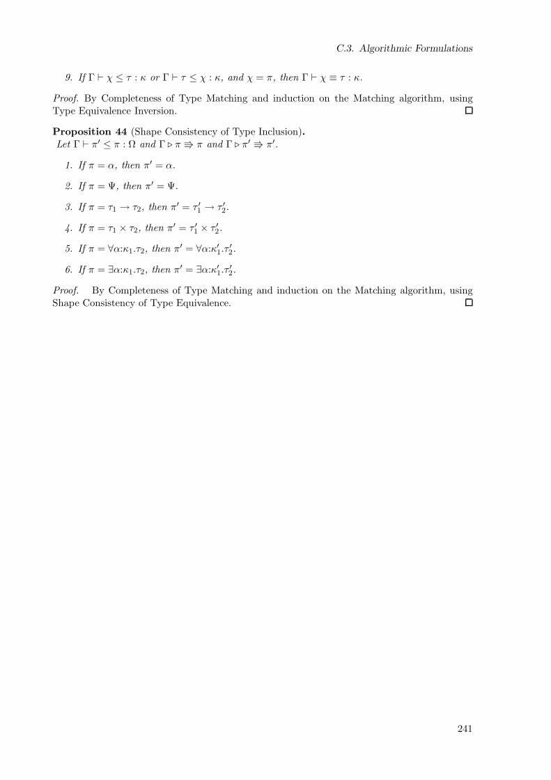
C.3. Algorithmic Formulations
9. If Γ ⊢ χ ≤ τ : κ or Γ ⊢ τ ≤ χ : κ, and χ = π, then Γ ⊢ χ ≡ τ : κ.
Proof. By Completeness of Type Matching and induction on the Matching algorithm, usingType Equivalence Inversion.
Proposition 44 (Shape Consistency of Type Inclusion).Let Γ ⊢ π′ ≤ π : Ω and Γ ⊲ π π and Γ ⊲ π′ π′.
1. If π = α, then π′ = α.
2. If π = Ψ, then π′ = Ψ.
3. If π = τ1 → τ2, then π′ = τ ′1 → τ ′2.
4. If π = τ1 × τ2, then π′ = τ ′1 × τ ′2.
5. If π = ∀α:κ1.τ2, then π′ = ∀α:κ′1.τ′2.
6. If π = ∃α:κ1.τ2, then π′ = ∃α:κ′1.τ′2.
Proof. By Completeness of Type Matching and induction on the Matching algorithm, usingShape Consistency of Type Equivalence.
241
C. Proofs of Type Level Properties
242
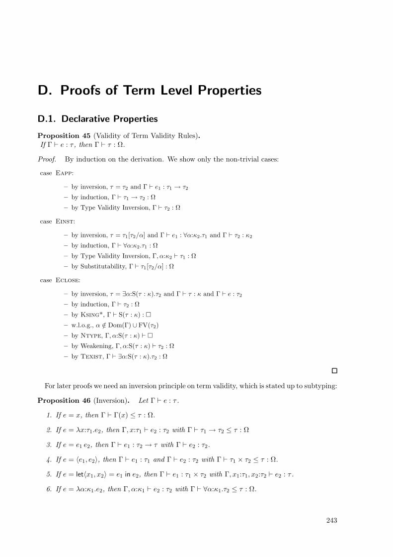
D. Proofs of Term Level Properties
D.1. Declarative Properties
Proposition 45 (Validity of Term Validity Rules).If Γ ⊢ e : τ , then Γ ⊢ τ : Ω.
Proof. By induction on the derivation. We show only the non-trivial cases:
case Eapp:
– by inversion, τ = τ2 and Γ ⊢ e1 : τ1 → τ2
– by induction, Γ ⊢ τ1 → τ2 : Ω
– by Type Validity Inversion, Γ ⊢ τ2 : Ω
case Einst:
– by inversion, τ = τ1[τ2/α] and Γ ⊢ e1 : ∀α:κ2.τ1 and Γ ⊢ τ2 : κ2
– by induction, Γ ⊢ ∀α:κ2.τ1 : Ω
– by Type Validity Inversion, Γ, α:κ2 ⊢ τ1 : Ω
– by Substitutability, Γ ⊢ τ1[τ2/α] : Ω
case Eclose:
– by inversion, τ = ∃α:S(τ : κ).τ2 and Γ ⊢ τ : κ and Γ ⊢ e : τ2
– by induction, Γ ⊢ τ2 : Ω
– by Ksing*, Γ ⊢ S(τ : κ) :
– w.l.o.g., α /∈ Dom(Γ) ∪ FV(τ2)
– by Ntype, Γ, α:S(τ : κ) ⊢
– by Weakening, Γ, α:S(τ : κ) ⊢ τ2 : Ω
– by Texist, Γ ⊢ ∃α:S(τ : κ).τ2 : Ω
For later proofs we need an inversion principle on term validity, which is stated up to subtyping:
Proposition 46 (Inversion). Let Γ ⊢ e : τ .
1. If e = x, then Γ ⊢ Γ(x) ≤ τ : Ω.
2. If e = λx:τ1.e2, then Γ, x:τ1 ⊢ e2 : τ2 with Γ ⊢ τ1 → τ2 ≤ τ : Ω
3. If e = e1 e2, then Γ ⊢ e1 : τ2 → τ with Γ ⊢ e2 : τ2.
4. If e = 〈e1, e2〉, then Γ ⊢ e1 : τ1 and Γ ⊢ e2 : τ2 with Γ ⊢ τ1 × τ2 ≤ τ : Ω.
5. If e = let〈x1, x2〉 = e1 in e2, then Γ ⊢ e1 : τ1 × τ2 with Γ, x1:τ1, x2:τ2 ⊢ e2 : τ .
6. If e = λα:κ1.e2, then Γ, α:κ1 ⊢ e2 : τ2 with Γ ⊢ ∀α:κ1.τ2 ≤ τ : Ω.
243
D. Proofs of Term Level Properties
7. If e = e1 τ2, then Γ ⊢ e1 : ∀α:κ2.τ1 with Γ ⊢ τ2 : κ2 and Γ ⊢ τ1[τ2/α] ≤ τ : Ω.
8. If e = 〈τ1, e2〉, then Γ ⊢ τ1 : κ1 and Γ ⊢ e2 : τ2 and Γ ⊢ ∃α:S(τ1 : κ1).τ2 ≤ τ : Ω.
9. If e = let〈α, x〉 = e1 inτ2 e2, then Γ ⊢ e1 : ∃α:κ1.τ2 and Γ, α:κ1, x:τ2 ⊢ e2 : τ2 andΓ ⊢ τ2 ≤ τ : Ω.
10. If e = newα ≈ τ1 inτ2 e2, then Γ, α:A(τ1) ⊢ e2 : τ2 and Γ ⊢ τ2 ≤ τ : Ω.
11. If e = e1+τ2 , then Γ ⊢ e1 : τ1 with Γ ⊢ τ2 : A(τ1) and Γ ⊢ τ2 ≤ τ : Ω.
12. If e = e1−τ1 , then Γ ⊢ e1 : τ1 with Γ ⊢ τ1 : A(τ2) and Γ ⊢ τ2 ≤ τ : Ω.
13. If e = case e1:τ1 of x:τ2.e2 elseτ2 e3, then Γ ⊢ e1 : τ1 and Γ, x:τ2 ⊢ e2 : τ2 and Γ ⊢ e3 : τ2and Γ ⊢ τ2 ≤ τ : Ω.
14. If e = pickle e1, then Γ ⊢ e1 : ∃α:Ω.α and Γ ⊢ Ψ ≤ τ : Ω.
15. If e = ψ(v), then FV(v) ⊆ Dom(Γ) and Γ ⊢ Ψ ≤ τ : Ω.
16. If e = unpicklex ⇐ e1 in e2 elseτ2 e3, then Γ ⊢ e1 : Ψ and Γ, x:∃α:Ω.α ⊢ e2 : τ2 andΓ ⊢ e3 : τ2 and Γ ⊢ τ2 ≤ τ : Ω.
Proof. Each by easy induction on the derivation. We show only a few representative cases:
1. e = x
case Evar: τ = Γ(x):
– by inversion, Γ ⊢
– by Environment Validity, Γ1 ⊢ Γ(x) : Ω with Γ = Γ1, x:Γ(x),Γ2
– by Weakening, Γ ⊢ Γ(x) : Ω
– by Reflexivity, Γ ⊢ Γ(x) ≤ τ : Ω
case Esub:
– by inversion, Γ ⊢ e : τ ′ and Γ ⊢ τ ′ ≤ τ : Ω
– by induction, Γ ⊢ Γ(x) ≤ τ ′ : Ω
– by Transitivity, Γ ⊢ Γ(x) ≤ τ : Ω
3. e = e1 e2
case Eapp:
– by inversion, Γ ⊢ e1 : τ2 → τ and Γ ⊢ e2 : τ2 directly
case Esub:
– by inversion, Γ ⊢ e : τ ′ and Γ ⊢ τ ′ ≤ τ : Ω
– by induction, Γ ⊢ e1 : τ2 → τ ′ and Γ ⊢ e2 : τ2
– by Validity and Reflexivity, Γ ⊢ τ2 ≤ τ2 : Ω
– by TSarrow, Γ ⊢ τ2 → τ ′ ≤ τ2 → τ : Ω
– by Esub, Γ ⊢ e1 : τ2 → τ
11. e = e1+τ
case Eup: τ = τ2
– by inversion, Γ ⊢ e1 : τ1 and Γ ⊢ τ2 : A(τ1)
– by Validity, Γ ⊢ τ1 : Ω
– by KSabs, Γ ⊢ A(τ1) ≤ Ω :
244
D.2. Algorithmic Type Checking
– by Tsub, Γ ⊢ τ2 : Ω
– by Validity and Reflexivity, Γ ⊢ τ2 ≤ τ : Ω
case Esub:
– by inversion, Γ ⊢ e : τ ′ and Γ ⊢ τ ′ ≤ τ : Ω
– by induction, Γ ⊢ e1 : τ1 and Γ ⊢ τ2 : A(τ1) and Γ ⊢ τ2 ≤ τ ′ : Ω
– by Transitivity, Γ ⊢ τ2 ≤ τ : Ω
16. e = unpicklex⇐ e1 in e2 elseτ2 e3
case Eunpickle: τ = τ2
– by inversion, Γ ⊢ e1 : Ψ and Γ, x:∃α:Ω.α ⊢ e2 : τ2 and Γ ⊢ e3 : τ2
– by Reflexivity, Γ ⊢ τ2 ≤ τ2 : Ω
case Esub:
– by inversion, Γ ⊢ e : τ ′ and Γ ⊢ τ ′ ≤ τ : Ω
– by induction, Γ ⊢ e1 : Ψ and Γ, x:∃α:Ω.α ⊢ e2 : τ2 and Γ ⊢ e3 : τ2 and Γ ⊢ τ2 ≤ τ ′ : Ω
– by Transitivity, Γ ⊢ τ2 ≤ τ : Ω
D.2. Algorithmic Type Checking
Theorem 47 (Soundness of Algorithmic Type Synthesis).Let Γ ⊢ .
1. If Γ ⊲ e τ , then Γ ⊢ e : τ .
2. If Γ ⊲ e π, then Γ ⊢ e : π.
3. If Γ ⊲ e τ with Γ ⊢ τ : Ω, then Γ ⊢ e : τ .
Proof. By easy simultaneous induction on the derivation, using Soundness of Algorithmic KindSynthesis. We show only a few representative cases:
1. case e = λx:τ1.e2
– by inversion, Γ ⊲ τ1 Ω and Γ, x:τ1 ⊲ e2 τ2
– by Soundness of Kind Synthesis, Γ ⊢ τ1 : Ω
– w.l.o.g., x /∈ Dom(Γ)
– by Nterm, Γ, x:τ1 ⊢
– by induction, Γ, x:τ1 ⊢ e2 : τ2
– by Elambda, Γ ⊢ λx:τ1.e2 : τ1 → τ2
case e = e1 e2
– by inversion, Γ ⊲ e1 τ2 → τ1 and Γ ⊲ e2 τ2
– by induction (2), Γ ⊢ e1 : τ2 → τ1
– by Validity, Γ ⊢ τ2 → τ1 : Ω
– by Type Validity Inversion, Γ ⊢ τ2 : Ω
– by induction (3), Γ ⊢ e2 : τ2
– by Eapp, Γ ⊢ e1 e2 : τ1
case e = e+τ1
– by inversion, Γ ⊲ τ1 SA(τ2)(τ3) and Γ ⊲ e2 τ2
– by Soundness of Kind Synthesis, Γ ⊢ τ1 : SA(τ2)(τ3)
245
D. Proofs of Term Level Properties
– by Kind Subsumption, Γ ⊢ τ1 : A(τ2)
– by Validity, Γ ⊢ A(τ2) :
– by inverting Kabs, Γ ⊢ τ2 : Ω
– by induction (3), Γ ⊢ e : τ2
– by Eup, Γ ⊢ e+τ1
: τ1
2. • by inversion, Γ ⊲ e τ and Γ ⊲ τ π
• by induction (1), Γ ⊢ e : τ
• by Soundness of Type Comparison, Γ ⊢ τ ≡ π : Ω
• by TSequiv, Γ ⊢ τ ≤ π : Ω
• by Esub, Γ ⊢ e : π
3. • by inversion, Γ ⊲ e τ ′ and Γ ⊲ τ ′ ≤ τ Ω
• by induction (1), Γ ⊢ e : τ ′
• by Validity, Γ ⊢ τ ′ : Ω and Γ ⊢ Ω :
• by Soundness of Type Matching, Γ ⊢ τ ′ ≤ τ : Ω
• by Esub, Γ ⊢ e : τ
Theorem 48 (Completeness of Algorithmic Type Synthesis).
1. If Γ ⊢ e : τ , then Γ ⊲ e τ ′ with Γ ⊢ τ ′ ≤ τ : Ω.
2. If Γ ⊢ e : τ , then Γ ⊲ e π with Γ ⊢ π ≤ τ : Ω.
3. If Γ ⊢ e : τ and Γ ⊢ τ ≤ τ ′ : Ω, then Γ ⊲ e τ ′.
Proof. By simultaneous induction on the derivation, using Completeness of Algorithmic KindSynthesis. We show only a few representative cases:
1. case Elambda:
– by inversion, Γ, x:τ1 ⊢ e2 : τ2
– by Environment Validity, Γ, x:τ1 ⊢ and Γ ⊢ τ1 : Ω
– by Completeness of Kind Synthesis, Γ ⊲ τ1 Ω
– by induction, Γ, x:τ1 ⊲ e2 τ ′2 with Γ ⊢ τ ′2 ≤ τ2 : Ω
– by rule, Γ ⊲ λx:τ1.e2 : τ1 → τ ′2– by Reflexivity, Γ ⊢ τ1 ≤ τ1 : Ω
– by TSarrow, Γ ⊢ τ1 → τ ′2 ≤ τ1 → τ2 : Ω
case Eapp:
– by inversion, Γ ⊢ e1 : τ2 → τ and Γ ⊢ e2 : τ2
– by induction (2), Γ ⊲ e1 π with Γ ⊢ π ≤ τ2 → τ : Ω
– by Shape Consistency of Type Inclusion, π = τ ′2 → τ ′
– by Type Inclusion Inversion, Γ ⊢ τ2 ≤ τ ′2 : Ω and Γ ⊢ τ ′ ≤ τ : Ω
– by induction (3), Γ ⊲ e2 τ ′2– by rule, Γ ⊲ e1 e2 τ ′
case Eup:
– by inversion, Γ ⊢ τ1 : A(τ2) and Γ ⊢ e : τ2
– by inspection of Kind Inclusion, the only proper subkinds of A(τ2) are of the formSA(τ ′
2)(τ3)
246
D.3. Soundness
– by Completeness of Kind Synthesis, Γ ⊲ τ1 SA(τ ′2)(τ3) and Γ ⊢ SA(τ ′
2)(τ3) ≤ A(τ2) :
– by inverting KSsing-left, Γ ⊢ A(τ ′2) ≤ A(τ2) :
– by inverting KSabs, Γ ⊢ τ ′2 ≡ τ2 :
– by Antisymmetry, Γ ⊢ τ2 ≤ τ ′2 : Ω
– by induction (3), Γ ⊲ e τ ′2– by rule, Γ ⊲ e+
τ1 τ1
– by Reflexivity, Γ ⊢ τ1 ≤ τ1 : Ω
2. • by induction (1), Γ ⊲ e τ ′ with Γ ⊢ τ ′ ≤ τ : Ω
• by Validity, Γ ⊢ τ ′ : Ω and Γ ⊢ τ : Ω
• by Completeness of Type Comparison, Γ ⊲ τ ′ π
• by rule, Γ ⊲ e π
• by Soundness of Type Comparison, Γ ⊢ τ ′ ≡ π : Ω
• by Antisymmetry and Transitivity, Γ ⊢ π ≤ τ : Ω
3. • by induction (1), Γ ⊲ e τ ′′ with Γ ⊢ τ ′′ ≤ τ : Ω
• by Transitivity, Γ ⊢ τ ′′ ≤ τ ′ : Ω
• by Validity, Γ ⊢ τ ′′ : Ω and Γ ⊢ τ ′ : Ω
• by Completeness of Type Matching, Γ ⊲ τ ′′ ≤ τ ′ Ω
• by rule, Γ ⊲ e τ ′
D.3. Soundness
D.3.1. Preservation
For showing preservation of cancelled coercions, it is important to know that two abstract typesthat are known to be equal at kind Ω are actually the same abstract type, with the samerepresentation:
Proposition 49 (Representation Equivalence).Let Γ ⊢ τ1 : A(τ ′1) and Γ ⊢ τ2 : A(τ ′2).
1. If Γ ⊢ τ1 ≡ τ2 : Ω, then Γ ⊢ τ1 ≡ τ2 : A(τ ′1) and Γ ⊢ τ ′1 ≡ τ ′2 : Ω.
2. If Γ ⊢ τ1 ≤ τ2 : Ω, then Γ ⊢ τ1 ≡ τ2 : A(τ ′1) and Γ ⊢ τ ′1 ≡ τ ′2 : Ω.
Proof.
1. • by Completeness of Type Comparison, Γ ⊢ τ1 τ and Γ ⊢ τ2 τ
• by Soundness of Type Comparison, Γ ⊢ τ1 ≡ τ : A(τ ′1) and Γ ⊢ τ2 ≡ τ : A(τ ′2)
• by Validity, Γ ⊢ τ : A(τ ′1) and Γ ⊢ τ : A(τ ′2)
• by Completeness of Kind Synthesis, Γ ⊢ τ : A(τ ′) with Γ ⊢ A(τ ′) ≤ A(τ ′1) : and Γ ⊢A(τ ′) ≤ A(τ ′2) :
• by inverting KSabs, Γ ⊢ τ ′ ≡ τ ′1 : Ω and Γ ⊢ τ ′ ≡ τ ′2 : Ω
• by Symmetry and Transitivity, Γ ⊢ τ ′2 ≡ τ ′1 : Ω
• by KSabs, Γ ⊢ A(τ ′2) ≤ A(τ ′1) :
• by Tsub, Γ ⊢ τ2 : A(τ ′1)
• by definition of Type Comparison, Γ ⊲ τ1 ≡ τ2 A(τ1)
247

D. Proofs of Term Level Properties
• by Soundness of Type Comparison, Γ ⊢ τ1 ≡ τ2 : A(τ1)
2. • by Completeness of Type Comparison, Γ ⊲ τ1 π1 and Γ ⊲ τ2 π2
• by Soundness of Type Comparison, Γ ⊢ τ1 ≡ π1 : A(τ ′1) and Γ ⊢ τ2 ≡ π2 : A(τ ′2)
• by Validity, Γ ⊢ π1 : A(τ ′1) and Γ ⊢ π2 : A(τ ′2)
• by Canonical Types, π1 = χ1 and π2 = χ2
• by Kind Subsumption, Γ ⊢ τ1 ≡ π1 : Ω and Γ ⊢ τ2 ≡ π2 : Ω
• by Symmetry, TSequiv, and Transitivity, Γ ⊢ π1 ≤ π2 : Ω
• by Type Inclusion Inversion, Γ ⊢ π1 ≡ π2 : Ω
• by Transitivity, Γ ⊢ τ1 ≡ τ2 : Ω
• by (1), Γ ⊢ τ1 ≡ τ2 : A(τ ′1) and Γ ⊢ τ ′1 ≡ τ ′2 : Ω
Lemma 50 (Decomposition and Replacement). If Γ ⊢ E[e] : τ , then Γ ⊢ e : τ ′, and ifΓ′ ⊢ e′ : τ ′ with Γ′ ⊇ Γ then Γ′ ⊢ E[e′] : τ .
Proof. By straightforward induction on the structure of the context, using Inversion.
Theorem 51 (Preservation).
1. If ∆ ⊢ e : τ and ∆; e→ ∆′; e′ with E = , then ∆′ ⊢ e′ : τ .
2. If · ⊢ C : τ and C → C ′, then · ⊢ C ′ : τ .
Proof. 1. Case analysis:
case Rapp: e = (λx:τ1.e2) v and e′ = e2[v/x]
– by Inversion (3), ∆ ⊢ λx:τ1.e2 : τ ′1 → τ ′′ and ∆ ⊢ v : τ ′1– by Inversion (2), ∆, x:τ1 ⊢ e2 : τ2 and ∆ ⊢ τ1 → τ2 ≤ τ ′1 → τ : Ω
– by Type Inclusion Inversion, ∆ ⊢ τ ′1 ≤ τ1 : Ω and ∆ ⊢ τ2 ≤ τ : Ω
– by Weakening, ∆, x:τ1 ⊢ τ2 ≤ τ : Ω
– by Esub, ∆ ⊢ v : τ1 and ∆, x:τ1 ⊢ e2 : τ
– by Substitutability, ∆ ⊢ e2[v/x] : τ
case Rproj: e = let〈x1, x2〉=〈v1, v2〉 in e2 and e′ = e2[v1/x1][v2/x2]
– by Inversion (5), ∆ ⊢ 〈v1, v2〉 : τ1 × τ2 and ∆, x1:τ1, x2:τ2 ⊢ e2 : τ
– by Inversion (4), ∆ ⊢ v1 : τ ′1 and ∆ ⊢ v2 : τ ′2 and ∆ ⊢ τ ′1 × τ ′2 ≤ τ1 × τ2 : Ω
– by Type Inclusion Inversion, ∆ ⊢ τ ′1 ≤ τ1 : Ω and ∆ ⊢ τ ′2 ≤ τ2 : Ω
– by Esub, ∆ ⊢ v1 : τ1 and ∆ ⊢ v2 : τ2– by Substitutability, ∆ ⊢ e2[v1/x1][v2/x2] : τ
case Rinst: e = (λα:κ1.e2) τ3 and e′ = e2[τ3/α]
– by Inversion (7), ∆ ⊢ λα:κ1.e2 : ∀α:κ′1.τ′2 and ∆ ⊢ τ3 : κ′1 and ∆ ⊢ τ ′2[τ3/α] ≤ τ : Ω
– by Inversion (6), ∆, α:κ1 ⊢ e2 : τ2 and ∆ ⊢ ∀α:κ1.τ2 ≤ ∀α:κ′1.τ′2 : Ω
– by Type Inclusion Inversion, ∆ ⊢ κ′1 ≤ κ1 : Ω and ∆, α:κ′1 ⊢ τ2 ≤ τ ′2 : Ω
– by Substitutability, ∆ ⊢ τ2[τ3/α] ≤ τ ′2[τ3/α] : Ω
– by Tsub, ∆ ⊢ τ3 : κ1
– by Substitutability, ∆ ⊢ e2[τ3/α] : τ2[τ3/α]
– by Esub, ∆ ⊢ e2[τ3/α] : τ ′2[τ3/α]
– by Esub, ∆ ⊢ e2[τ3/α] : τ
248
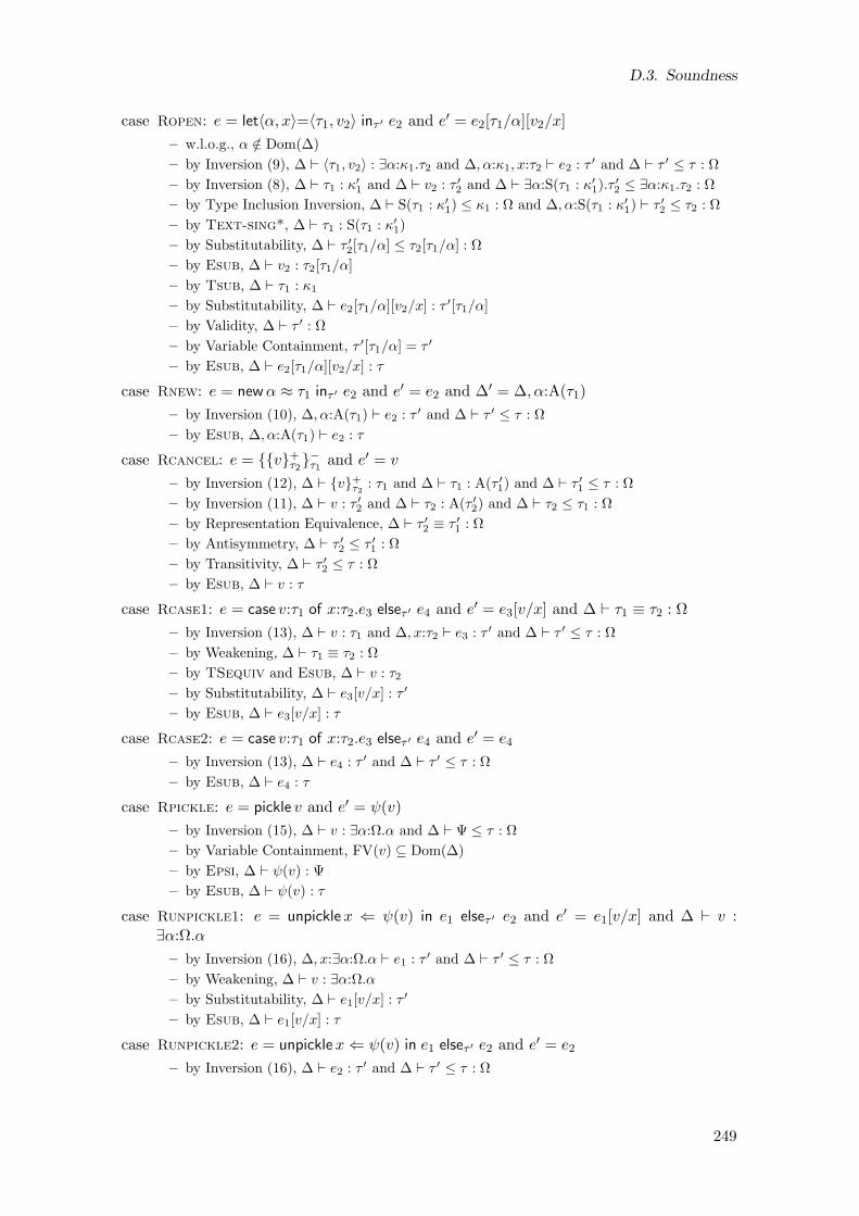
D.3. Soundness
case Ropen: e = let〈α, x〉=〈τ1, v2〉 inτ ′ e2 and e′ = e2[τ1/α][v2/x]
– w.l.o.g., α /∈ Dom(∆)
– by Inversion (9), ∆ ⊢ 〈τ1, v2〉 : ∃α:κ1.τ2 and ∆, α:κ1, x:τ2 ⊢ e2 : τ ′ and ∆ ⊢ τ ′ ≤ τ : Ω
– by Inversion (8), ∆ ⊢ τ1 : κ′1 and ∆ ⊢ v2 : τ ′2 and ∆ ⊢ ∃α:S(τ1 : κ′1).τ′2 ≤ ∃α:κ1.τ2 : Ω
– by Type Inclusion Inversion, ∆ ⊢ S(τ1 : κ′1) ≤ κ1 : Ω and ∆, α:S(τ1 : κ′1) ⊢ τ′2 ≤ τ2 : Ω
– by Text-sing*, ∆ ⊢ τ1 : S(τ1 : κ′1)
– by Substitutability, ∆ ⊢ τ ′2[τ1/α] ≤ τ2[τ1/α] : Ω
– by Esub, ∆ ⊢ v2 : τ2[τ1/α]
– by Tsub, ∆ ⊢ τ1 : κ1
– by Substitutability, ∆ ⊢ e2[τ1/α][v2/x] : τ ′[τ1/α]
– by Validity, ∆ ⊢ τ ′ : Ω
– by Variable Containment, τ ′[τ1/α] = τ ′
– by Esub, ∆ ⊢ e2[τ1/α][v2/x] : τ
case Rnew: e = newα ≈ τ1 inτ ′ e2 and e′ = e2 and ∆′ = ∆, α:A(τ1)
– by Inversion (10), ∆, α:A(τ1) ⊢ e2 : τ ′ and ∆ ⊢ τ ′ ≤ τ : Ω
– by Esub, ∆, α:A(τ1) ⊢ e2 : τ
case Rcancel: e = v+τ2
−τ1 and e′ = v
– by Inversion (12), ∆ ⊢ v+τ2
: τ1 and ∆ ⊢ τ1 : A(τ ′1) and ∆ ⊢ τ ′1 ≤ τ : Ω
– by Inversion (11), ∆ ⊢ v : τ ′2 and ∆ ⊢ τ2 : A(τ ′2) and ∆ ⊢ τ2 ≤ τ1 : Ω
– by Representation Equivalence, ∆ ⊢ τ ′2 ≡ τ ′1 : Ω
– by Antisymmetry, ∆ ⊢ τ ′2 ≤ τ ′1 : Ω
– by Transitivity, ∆ ⊢ τ ′2 ≤ τ : Ω
– by Esub, ∆ ⊢ v : τ
case Rcase1: e = case v:τ1 of x:τ2.e3 elseτ ′ e4 and e′ = e3[v/x] and ∆ ⊢ τ1 ≡ τ2 : Ω
– by Inversion (13), ∆ ⊢ v : τ1 and ∆, x:τ2 ⊢ e3 : τ ′ and ∆ ⊢ τ ′ ≤ τ : Ω
– by Weakening, ∆ ⊢ τ1 ≡ τ2 : Ω
– by TSequiv and Esub, ∆ ⊢ v : τ2
– by Substitutability, ∆ ⊢ e3[v/x] : τ ′
– by Esub, ∆ ⊢ e3[v/x] : τ
case Rcase2: e = case v:τ1 of x:τ2.e3 elseτ ′ e4 and e′ = e4
– by Inversion (13), ∆ ⊢ e4 : τ ′ and ∆ ⊢ τ ′ ≤ τ : Ω
– by Esub, ∆ ⊢ e4 : τ
case Rpickle: e = pickle v and e′ = ψ(v)
– by Inversion (15), ∆ ⊢ v : ∃α:Ω.α and ∆ ⊢ Ψ ≤ τ : Ω
– by Variable Containment, FV(v) ⊆ Dom(∆)
– by Epsi, ∆ ⊢ ψ(v) : Ψ
– by Esub, ∆ ⊢ ψ(v) : τ
case Runpickle1: e = unpicklex ⇐ ψ(v) in e1 elseτ ′ e2 and e′ = e1[v/x] and ∆ ⊢ v :∃α:Ω.α
– by Inversion (16), ∆, x:∃α:Ω.α ⊢ e1 : τ ′ and ∆ ⊢ τ ′ ≤ τ : Ω
– by Weakening, ∆ ⊢ v : ∃α:Ω.α
– by Substitutability, ∆ ⊢ e1[v/x] : τ ′
– by Esub, ∆ ⊢ e1[v/x] : τ
case Runpickle2: e = unpicklex⇐ ψ(v) in e1 elseτ ′ e2 and e′ = e2
– by Inversion (16), ∆ ⊢ e2 : τ ′ and ∆ ⊢ τ ′ ≤ τ : Ω
249
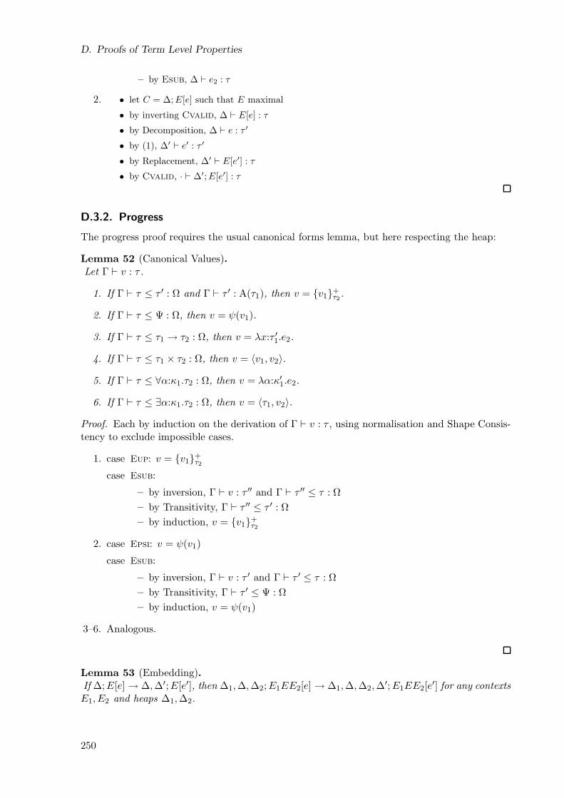
D. Proofs of Term Level Properties
– by Esub, ∆ ⊢ e2 : τ
2. • let C = ∆;E[e] such that E maximal
• by inverting Cvalid, ∆ ⊢ E[e] : τ
• by Decomposition, ∆ ⊢ e : τ ′
• by (1), ∆′ ⊢ e′ : τ ′
• by Replacement, ∆′ ⊢ E[e′] : τ
• by Cvalid, · ⊢ ∆′;E[e′] : τ
D.3.2. Progress
The progress proof requires the usual canonical forms lemma, but here respecting the heap:
Lemma 52 (Canonical Values).Let Γ ⊢ v : τ .
1. If Γ ⊢ τ ≤ τ ′ : Ω and Γ ⊢ τ ′ : A(τ1), then v = v1+τ2 .
2. If Γ ⊢ τ ≤ Ψ : Ω, then v = ψ(v1).
3. If Γ ⊢ τ ≤ τ1 → τ2 : Ω, then v = λx:τ ′1.e2.
4. If Γ ⊢ τ ≤ τ1 × τ2 : Ω, then v = 〈v1, v2〉.
5. If Γ ⊢ τ ≤ ∀α:κ1.τ2 : Ω, then v = λα:κ′1.e2.
6. If Γ ⊢ τ ≤ ∃α:κ1.τ2 : Ω, then v = 〈τ1, v2〉.
Proof. Each by induction on the derivation of Γ ⊢ v : τ , using normalisation and Shape Consis-tency to exclude impossible cases.
1. case Eup: v = v1+τ2
case Esub:
– by inversion, Γ ⊢ v : τ ′′ and Γ ⊢ τ ′′ ≤ τ : Ω
– by Transitivity, Γ ⊢ τ ′′ ≤ τ ′ : Ω
– by induction, v = v1+τ2
2. case Epsi: v = ψ(v1)
case Esub:
– by inversion, Γ ⊢ v : τ ′ and Γ ⊢ τ ′ ≤ τ : Ω
– by Transitivity, Γ ⊢ τ ′ ≤ Ψ : Ω
– by induction, v = ψ(v1)
3–6. Analogous.
Lemma 53 (Embedding).If ∆;E[e] → ∆,∆′;E[e′], then ∆1,∆,∆2;E1EE2[e] → ∆1,∆,∆2,∆
′;E1EE2[e′] for any contexts
E1, E2 and heaps ∆1,∆2.
250
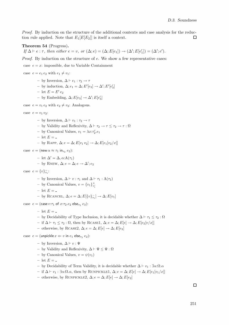
D.3. Soundness
Proof. By induction on the structure of the additional contexts and case analysis for the reduc-tion rule applied. Note that E1[E[E2]] is itself a context.
Theorem 54 (Progress).If ∆ ⊢ e : τ , then either e = v, or (∆; e) = (∆;E[e1]) → (∆′;E[e′1]) = (∆′; e′).
Proof. By induction on the structure of e. We show a few representative cases:
case e = x: impossible, due to Variable Containment
case e = e1 e2 with e1 6= v1:
– by Inversion, ∆ ⊢ e1 : τ2 → τ
– by induction, ∆; e1 = ∆;E′[e3] → ∆′;E′[e′3]
– let E = E′ e2
– by Embedding, ∆;E[e3] → ∆′;E[e′3]
case e = v1 e2 with e2 6= v2: Analogous.
case e = v1 v2:
– by Inversion, ∆ ⊢ v1 : τ2 → τ
– by Validity and Reflexivity, ∆ ⊢ τ2 → τ ≤ τ2 → τ : Ω
– by Canonical Values, v1 = λx:τ ′2.e1
– let E =
– by Rapp, ∆; e = ∆;E[v1 v2] → ∆;E[e1[v2/x]]
case e = (newα ≈ τ1 inτ2 e2):
– let ∆′ = ∆, α:A(τ1)
– by Rnew, ∆; e = ∆; e→ ∆′; e2
case e = v−τ1:
– by Inversion, ∆ ⊢ v : τ1 and ∆ ⊢ τ1 : A(τ2)
– by Canonical Values, v = v1+τ ′1
– let E =
– by Rcancel, ∆; e = ∆;E[v−τ1] → ∆;E[v1]
case e = (case v:τ1 of x:τ2.e2 elseτ2 e3):
– let E =
– by Decidability of Type Inclusion, it is decidable whether ∆ ⊢ τ1 ≤ τ2 : Ω
– if ∆ ⊢ τ1 ≤ τ2 : Ω, then by Rcase1, ∆; e = ∆;E[e] → ∆;E[e2[v/x]]
– otherwise, by Rcase2, ∆; e = ∆;E[e] → ∆;E[e3]
case e = (unpicklex⇐ v in e1 elseτ2 e2):
– by Inversion, ∆ ⊢ v : Ψ
– by Validity and Reflexivity, ∆ ⊢ Ψ ≤ Ψ : Ω
– by Canonical Values, v = ψ(v1)
– let E =
– by Decidability of Term Validity, it is decidable whether ∆ ⊢ v1 : ∃α:Ω.α
– if ∆ ⊢ v1 : ∃α:Ω.α, then by Runpickle1, ∆; e = ∆;E[e] → ∆;E[e1[v1/x]]
– otherwise, by Runpickle2, ∆; e = ∆;E[e] → ∆;E[e2]
251
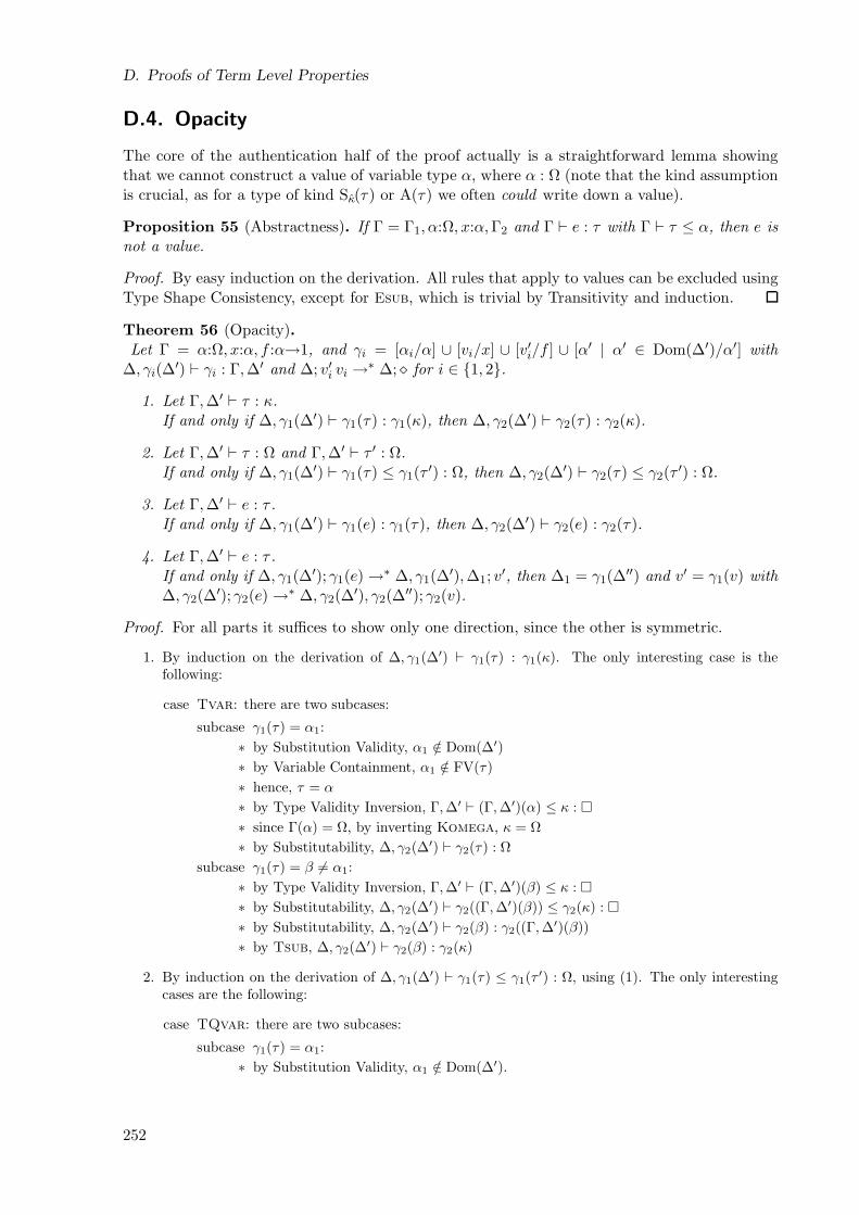
D. Proofs of Term Level Properties
D.4. Opacity
The core of the authentication half of the proof actually is a straightforward lemma showingthat we cannot construct a value of variable type α, where α : Ω (note that the kind assumptionis crucial, as for a type of kind Sκ(τ) or A(τ) we often could write down a value).
Proposition 55 (Abstractness). If Γ = Γ1, α:Ω, x:α,Γ2 and Γ ⊢ e : τ with Γ ⊢ τ ≤ α, then e isnot a value.
Proof. By easy induction on the derivation. All rules that apply to values can be excluded usingType Shape Consistency, except for Esub, which is trivial by Transitivity and induction.
Theorem 56 (Opacity).Let Γ = α:Ω, x:α, f :α→1, and γi = [αi/α] ∪ [vi/x] ∪ [v′i/f ] ∪ [α′ | α′ ∈ Dom(∆′)/α′] with
∆, γi(∆′) ⊢ γi : Γ,∆′ and ∆; v′i vi →
∗ ∆; ⋄ for i ∈ 1, 2.
1. Let Γ,∆′ ⊢ τ : κ.If and only if ∆, γ1(∆
′) ⊢ γ1(τ) : γ1(κ), then ∆, γ2(∆′) ⊢ γ2(τ) : γ2(κ).
2. Let Γ,∆′ ⊢ τ : Ω and Γ,∆′ ⊢ τ ′ : Ω.If and only if ∆, γ1(∆
′) ⊢ γ1(τ) ≤ γ1(τ′) : Ω, then ∆, γ2(∆
′) ⊢ γ2(τ) ≤ γ2(τ′) : Ω.
3. Let Γ,∆′ ⊢ e : τ .If and only if ∆, γ1(∆
′) ⊢ γ1(e) : γ1(τ), then ∆, γ2(∆′) ⊢ γ2(e) : γ2(τ).
4. Let Γ,∆′ ⊢ e : τ .If and only if ∆, γ1(∆
′); γ1(e) →∗ ∆, γ1(∆
′),∆1; v′, then ∆1 = γ1(∆
′′) and v′ = γ1(v) with∆, γ2(∆
′); γ2(e) →∗ ∆, γ2(∆
′), γ2(∆′′); γ2(v).
Proof. For all parts it suffices to show only one direction, since the other is symmetric.
1. By induction on the derivation of ∆, γ1(∆′) ⊢ γ1(τ) : γ1(κ). The only interesting case is the
following:
case Tvar: there are two subcases:
subcase γ1(τ) = α1:
∗ by Substitution Validity, α1 /∈ Dom(∆′)
∗ by Variable Containment, α1 /∈ FV(τ)
∗ hence, τ = α
∗ by Type Validity Inversion, Γ,∆′ ⊢ (Γ,∆′)(α) ≤ κ :
∗ since Γ(α) = Ω, by inverting Komega, κ = Ω
∗ by Substitutability, ∆, γ2(∆′) ⊢ γ2(τ) : Ω
subcase γ1(τ) = β 6= α1:
∗ by Type Validity Inversion, Γ,∆′ ⊢ (Γ,∆′)(β) ≤ κ :
∗ by Substitutability, ∆, γ2(∆′) ⊢ γ2((Γ,∆
′)(β)) ≤ γ2(κ) :
∗ by Substitutability, ∆, γ2(∆′) ⊢ γ2(β) : γ2((Γ,∆
′)(β))
∗ by Tsub, ∆, γ2(∆′) ⊢ γ2(β) : γ2(κ)
2. By induction on the derivation of ∆, γ1(∆′) ⊢ γ1(τ) ≤ γ1(τ
′) : Ω, using (1). The only interestingcases are the following:
case TQvar: there are two subcases:
subcase γ1(τ) = α1:
∗ by Substitution Validity, α1 /∈ Dom(∆′).
252
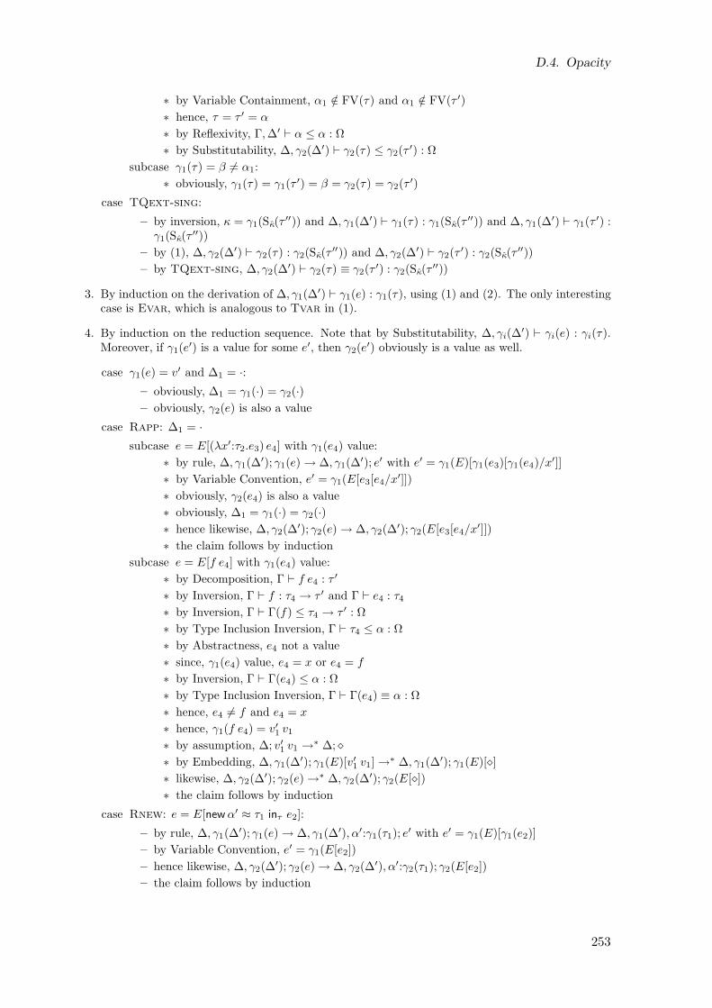
D.4. Opacity
∗ by Variable Containment, α1 /∈ FV(τ) and α1 /∈ FV(τ ′)
∗ hence, τ = τ ′ = α
∗ by Reflexivity, Γ,∆′ ⊢ α ≤ α : Ω
∗ by Substitutability, ∆, γ2(∆′) ⊢ γ2(τ) ≤ γ2(τ
′) : Ω
subcase γ1(τ) = β 6= α1:
∗ obviously, γ1(τ) = γ1(τ′) = β = γ2(τ) = γ2(τ
′)
case TQext-sing:
– by inversion, κ = γ1(Sκ(τ′′)) and ∆, γ1(∆
′) ⊢ γ1(τ) : γ1(Sκ(τ′′)) and ∆, γ1(∆
′) ⊢ γ1(τ′) :
γ1(Sκ(τ′′))
– by (1), ∆, γ2(∆′) ⊢ γ2(τ) : γ2(Sκ(τ
′′)) and ∆, γ2(∆′) ⊢ γ2(τ
′) : γ2(Sκ(τ′′))
– by TQext-sing, ∆, γ2(∆′) ⊢ γ2(τ) ≡ γ2(τ
′) : γ2(Sκ(τ′′))
3. By induction on the derivation of ∆, γ1(∆′) ⊢ γ1(e) : γ1(τ), using (1) and (2). The only interesting
case is Evar, which is analogous to Tvar in (1).
4. By induction on the reduction sequence. Note that by Substitutability, ∆, γi(∆′) ⊢ γi(e) : γi(τ).
Moreover, if γ1(e′) is a value for some e′, then γ2(e
′) obviously is a value as well.
case γ1(e) = v′ and ∆1 = ·:
– obviously, ∆1 = γ1(·) = γ2(·)
– obviously, γ2(e) is also a value
case Rapp: ∆1 = ·
subcase e = E[(λx′:τ2.e3) e4] with γ1(e4) value:
∗ by rule, ∆, γ1(∆′); γ1(e) → ∆, γ1(∆
′); e′ with e′ = γ1(E)[γ1(e3)[γ1(e4)/x′]]
∗ by Variable Convention, e′ = γ1(E[e3[e4/x′]])
∗ obviously, γ2(e4) is also a value
∗ obviously, ∆1 = γ1(·) = γ2(·)
∗ hence likewise, ∆, γ2(∆′); γ2(e) → ∆, γ2(∆
′); γ2(E[e3[e4/x′]])
∗ the claim follows by induction
subcase e = E[f e4] with γ1(e4) value:
∗ by Decomposition, Γ ⊢ f e4 : τ ′
∗ by Inversion, Γ ⊢ f : τ4 → τ ′ and Γ ⊢ e4 : τ4∗ by Inversion, Γ ⊢ Γ(f) ≤ τ4 → τ ′ : Ω
∗ by Type Inclusion Inversion, Γ ⊢ τ4 ≤ α : Ω
∗ by Abstractness, e4 not a value
∗ since, γ1(e4) value, e4 = x or e4 = f
∗ by Inversion, Γ ⊢ Γ(e4) ≤ α : Ω
∗ by Type Inclusion Inversion, Γ ⊢ Γ(e4) ≡ α : Ω
∗ hence, e4 6= f and e4 = x
∗ hence, γ1(f e4) = v′1 v1
∗ by assumption, ∆; v′1 v1 →∗ ∆; ⋄
∗ by Embedding, ∆, γ1(∆′); γ1(E)[v′1 v1] →
∗ ∆, γ1(∆′); γ1(E)[⋄]
∗ likewise, ∆, γ2(∆′); γ2(e) →∗ ∆, γ2(∆
′); γ2(E[⋄])
∗ the claim follows by induction
case Rnew: e = E[newα′ ≈ τ1 inτ e2]:
– by rule, ∆, γ1(∆′); γ1(e) → ∆, γ1(∆
′), α′:γ1(τ1); e′ with e′ = γ1(E)[γ1(e2)]
– by Variable Convention, e′ = γ1(E[e2])
– hence likewise, ∆, γ2(∆′); γ2(e) → ∆, γ2(∆
′), α′:γ2(τ1); γ2(E[e2])
– the claim follows by induction
253
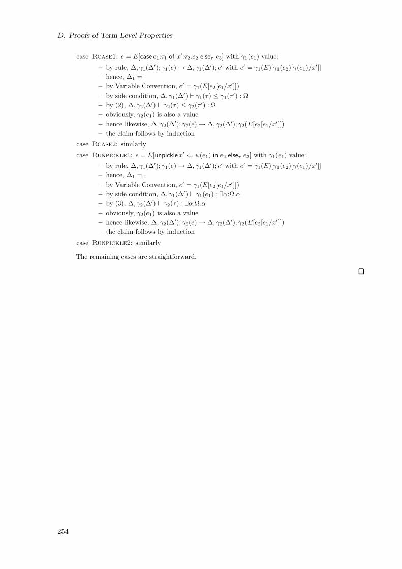
D. Proofs of Term Level Properties
case Rcase1: e = E[case e1:τ1 of x′:τ2.e2 elseτ e3] with γ1(e1) value:
– by rule, ∆, γ1(∆′); γ1(e) → ∆, γ1(∆
′); e′ with e′ = γ1(E)[γ1(e2)[γ(e1)/x′]]
– hence, ∆1 = ·
– by Variable Convention, e′ = γ1(E[e2[e1/x′]])
– by side condition, ∆, γ1(∆′) ⊢ γ1(τ) ≤ γ1(τ
′) : Ω
– by (2), ∆, γ2(∆′) ⊢ γ2(τ) ≤ γ2(τ
′) : Ω
– obviously, γ2(e1) is also a value
– hence likewise, ∆, γ2(∆′); γ2(e) → ∆, γ2(∆
′); γ2(E[e2[e1/x′]])
– the claim follows by induction
case Rcase2: similarly
case Runpickle1: e = E[unpicklex′ ⇐ ψ(e1) in e2 elseτ e3] with γ1(e1) value:
– by rule, ∆, γ1(∆′); γ1(e) → ∆, γ1(∆
′); e′ with e′ = γ1(E)[γ1(e2)[γ(e1)/x′]]
– hence, ∆1 = ·
– by Variable Convention, e′ = γ1(E[e2[e1/x′]])
– by side condition, ∆, γ1(∆′) ⊢ γ1(e1) : ∃α:Ω.α
– by (3), ∆, γ2(∆′) ⊢ γ2(τ) : ∃α:Ω.α
– obviously, γ2(e1) is also a value
– hence likewise, ∆, γ2(∆′); γ2(e) → ∆, γ2(∆
′); γ2(E[e2[e1/x′]])
– the claim follows by induction
case Runpickle2: similarly
The remaining cases are straightforward.
254
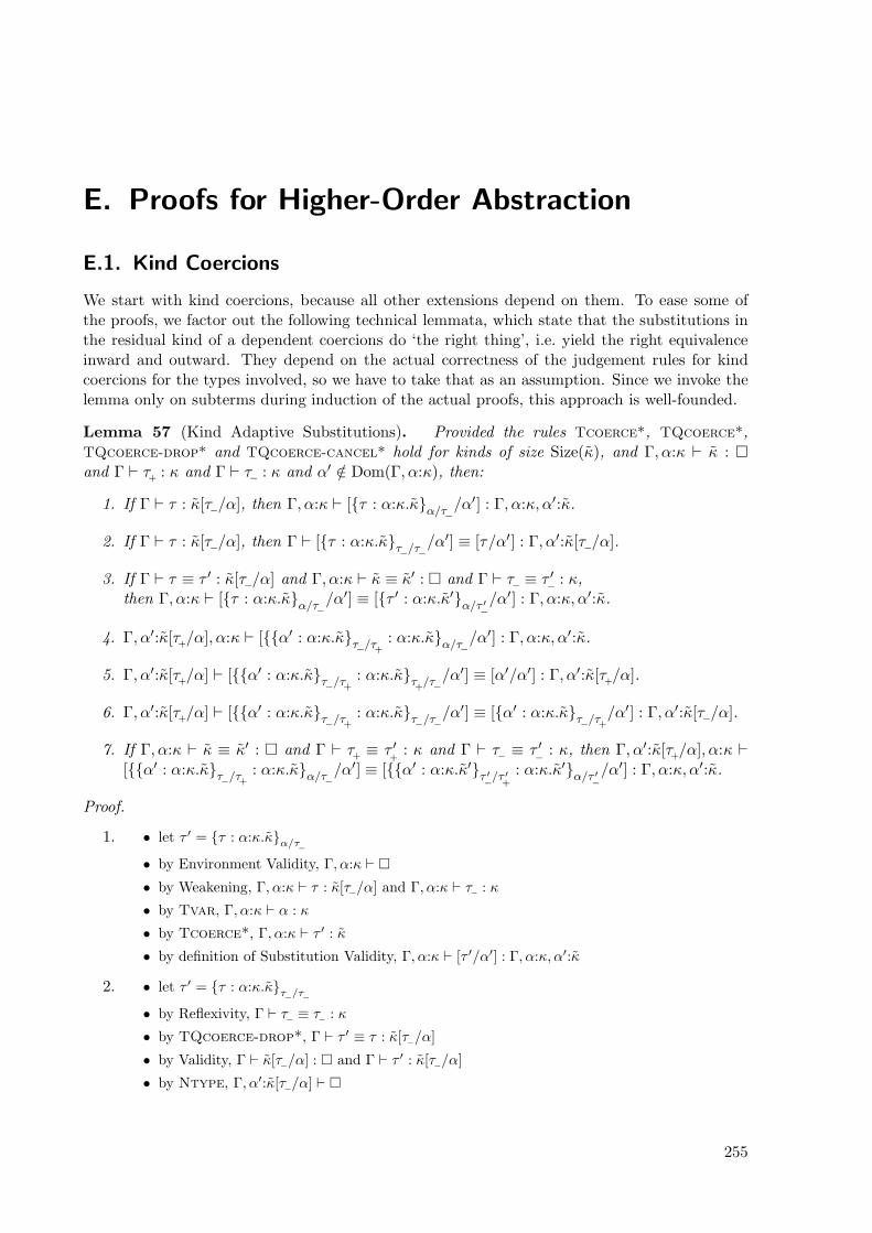
E. Proofs for Higher-Order Abstraction
E.1. Kind Coercions
We start with kind coercions, because all other extensions depend on them. To ease some ofthe proofs, we factor out the following technical lemmata, which state that the substitutions inthe residual kind of a dependent coercions do ‘the right thing’, i.e. yield the right equivalenceinward and outward. They depend on the actual correctness of the judgement rules for kindcoercions for the types involved, so we have to take that as an assumption. Since we invoke thelemma only on subterms during induction of the actual proofs, this approach is well-founded.
Lemma 57 (Kind Adaptive Substitutions). Provided the rules Tcoerce*, TQcoerce*,TQcoerce-drop* and TQcoerce-cancel* hold for kinds of size Size(κ), and Γ, α:κ ⊢ κ : and Γ ⊢ τ
+: κ and Γ ⊢ τ− : κ and α′ /∈ Dom(Γ, α:κ), then:
1. If Γ ⊢ τ : κ[τ−/α], then Γ, α:κ ⊢ [τ : α:κ.κα/τ−/α′] : Γ, α:κ, α′:κ.
2. If Γ ⊢ τ : κ[τ−/α], then Γ ⊢ [τ : α:κ.κτ−/τ−/α′] ≡ [τ/α′] : Γ, α′:κ[τ−/α].
3. If Γ ⊢ τ ≡ τ ′ : κ[τ−/α] and Γ, α:κ ⊢ κ ≡ κ′ : and Γ ⊢ τ− ≡ τ ′−
: κ,then Γ, α:κ ⊢ [τ : α:κ.κα/τ−
/α′] ≡ [τ ′ : α:κ.κ′α/τ ′−
/α′] : Γ, α:κ, α′:κ.
4. Γ, α′:κ[τ+/α], α:κ ⊢ [α′ : α:κ.κτ−/τ
+
: α:κ.κα/τ−/α′] : Γ, α:κ, α′:κ.
5. Γ, α′:κ[τ+/α] ⊢ [α′ : α:κ.κτ−/τ
+
: α:κ.κτ+
/τ−/α′] ≡ [α′/α′] : Γ, α′:κ[τ
+/α].
6. Γ, α′:κ[τ+/α] ⊢ [α′ : α:κ.κτ−/τ
+
: α:κ.κτ−/τ−/α′] ≡ [α′ : α:κ.κτ−/τ
+
/α′] : Γ, α′:κ[τ−/α].
7. If Γ, α:κ ⊢ κ ≡ κ′ : and Γ ⊢ τ+≡ τ ′
+: κ and Γ ⊢ τ− ≡ τ ′
−: κ, then Γ, α′:κ[τ
+/α], α:κ ⊢
[α′ : α:κ.κτ−/τ+
: α:κ.κα/τ−/α′] ≡ [α′ : α:κ.κ′τ ′
−/τ ′
+
: α:κ.κ′α/τ ′−
/α′] : Γ, α:κ, α′:κ.
Proof.
1. • let τ ′ = τ : α:κ.κα/τ−
• by Environment Validity, Γ, α:κ ⊢
• by Weakening, Γ, α:κ ⊢ τ : κ[τ−/α] and Γ, α:κ ⊢ τ− : κ
• by Tvar, Γ, α:κ ⊢ α : κ
• by Tcoerce*, Γ, α:κ ⊢ τ ′ : κ
• by definition of Substitution Validity, Γ, α:κ ⊢ [τ ′/α′] : Γ, α:κ, α′:κ
2. • let τ ′ = τ : α:κ.κτ−
/τ−
• by Reflexivity, Γ ⊢ τ− ≡ τ− : κ
• by TQcoerce-drop*, Γ ⊢ τ ′ ≡ τ : κ[τ−/α]
• by Validity, Γ ⊢ κ[τ−/α] : and Γ ⊢ τ ′ : κ[τ−/α]
• by Ntype, Γ, α′:κ[τ−/α] ⊢
255
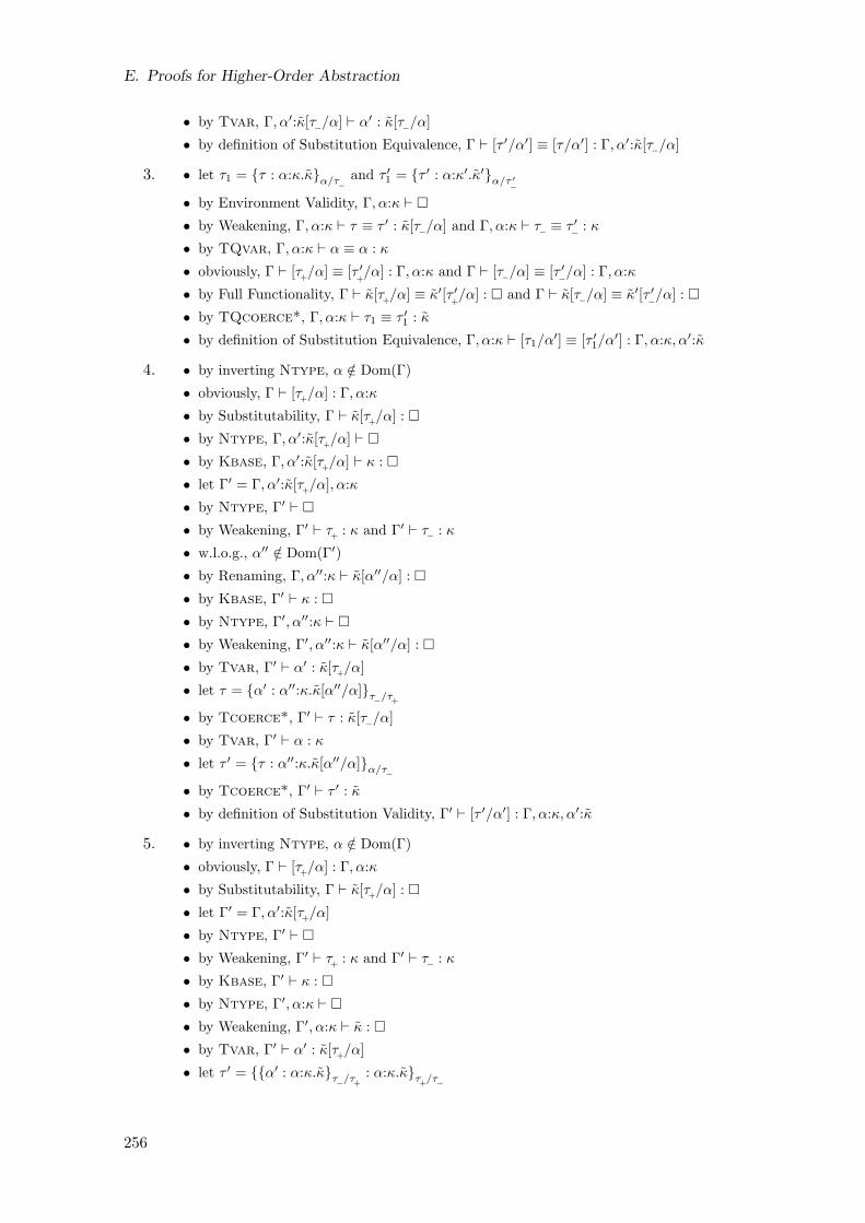
E. Proofs for Higher-Order Abstraction
• by Tvar, Γ, α′:κ[τ−/α] ⊢ α′ : κ[τ−/α]
• by definition of Substitution Equivalence, Γ ⊢ [τ ′/α′] ≡ [τ/α′] : Γ, α′:κ[τ−/α]
3. • let τ1 = τ : α:κ.κα/τ−and τ ′1 = τ ′ : α:κ′.κ′α/τ ′
−
• by Environment Validity, Γ, α:κ ⊢
• by Weakening, Γ, α:κ ⊢ τ ≡ τ ′ : κ[τ−/α] and Γ, α:κ ⊢ τ− ≡ τ ′−
: κ
• by TQvar, Γ, α:κ ⊢ α ≡ α : κ
• obviously, Γ ⊢ [τ+/α] ≡ [τ ′
+/α] : Γ, α:κ and Γ ⊢ [τ−/α] ≡ [τ ′
−/α] : Γ, α:κ
• by Full Functionality, Γ ⊢ κ[τ+/α] ≡ κ′[τ ′
+/α] : and Γ ⊢ κ[τ−/α] ≡ κ′[τ ′
−/α] :
• by TQcoerce*, Γ, α:κ ⊢ τ1 ≡ τ ′1 : κ
• by definition of Substitution Equivalence, Γ, α:κ ⊢ [τ1/α′] ≡ [τ ′1/α
′] : Γ, α:κ, α′:κ
4. • by inverting Ntype, α /∈ Dom(Γ)
• obviously, Γ ⊢ [τ+/α] : Γ, α:κ
• by Substitutability, Γ ⊢ κ[τ+/α] :
• by Ntype, Γ, α′:κ[τ+/α] ⊢
• by Kbase, Γ, α′:κ[τ+/α] ⊢ κ :
• let Γ′ = Γ, α′:κ[τ+/α], α:κ
• by Ntype, Γ′ ⊢
• by Weakening, Γ′ ⊢ τ+
: κ and Γ′ ⊢ τ− : κ
• w.l.o.g., α′′ /∈ Dom(Γ′)
• by Renaming, Γ, α′′:κ ⊢ κ[α′′/α] :
• by Kbase, Γ′ ⊢ κ :
• by Ntype, Γ′, α′′:κ ⊢
• by Weakening, Γ′, α′′:κ ⊢ κ[α′′/α] :
• by Tvar, Γ′ ⊢ α′ : κ[τ+/α]
• let τ = α′ : α′′:κ.κ[α′′/α]τ−/τ+
• by Tcoerce*, Γ′ ⊢ τ : κ[τ−/α]
• by Tvar, Γ′ ⊢ α : κ
• let τ ′ = τ : α′′:κ.κ[α′′/α]α/τ−
• by Tcoerce*, Γ′ ⊢ τ ′ : κ
• by definition of Substitution Validity, Γ′ ⊢ [τ ′/α′] : Γ, α:κ, α′:κ
5. • by inverting Ntype, α /∈ Dom(Γ)
• obviously, Γ ⊢ [τ+/α] : Γ, α:κ
• by Substitutability, Γ ⊢ κ[τ+/α] :
• let Γ′ = Γ, α′:κ[τ+/α]
• by Ntype, Γ′ ⊢
• by Weakening, Γ′ ⊢ τ+
: κ and Γ′ ⊢ τ− : κ
• by Kbase, Γ′ ⊢ κ :
• by Ntype, Γ′, α:κ ⊢
• by Weakening, Γ′, α:κ ⊢ κ :
• by Tvar, Γ′ ⊢ α′ : κ[τ+/α]
• let τ ′ = α′ : α:κ.κτ−
/τ+
: α:κ.κτ+
/τ−
256
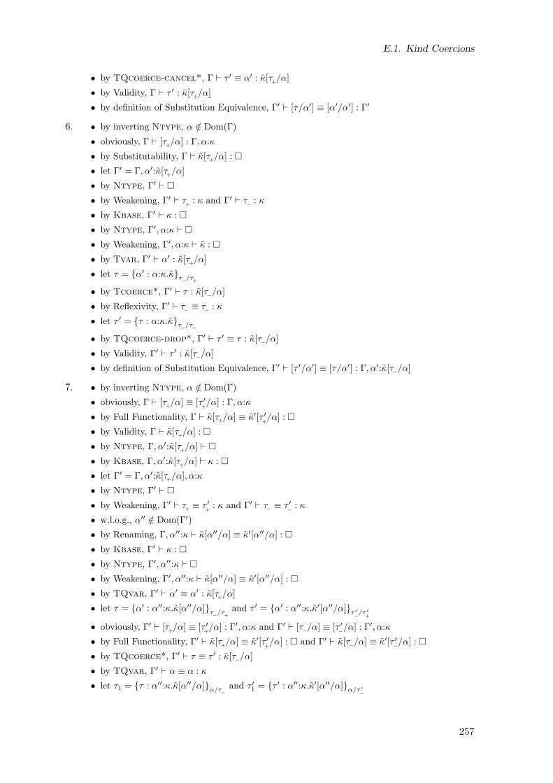
E.1. Kind Coercions
• by TQcoerce-cancel*, Γ ⊢ τ ′ ≡ α′ : κ[τ+/α]
• by Validity, Γ ⊢ τ ′ : κ[τ+/α]
• by definition of Substitution Equivalence, Γ′ ⊢ [τ/α′] ≡ [α′/α′] : Γ′
6. • by inverting Ntype, α /∈ Dom(Γ)
• obviously, Γ ⊢ [τ+/α] : Γ, α:κ
• by Substitutability, Γ ⊢ κ[τ+/α] :
• let Γ′ = Γ, α′:κ[τ+/α]
• by Ntype, Γ′ ⊢
• by Weakening, Γ′ ⊢ τ+
: κ and Γ′ ⊢ τ− : κ
• by Kbase, Γ′ ⊢ κ :
• by Ntype, Γ′, α:κ ⊢
• by Weakening, Γ′, α:κ ⊢ κ :
• by Tvar, Γ′ ⊢ α′ : κ[τ+/α]
• let τ = α′ : α:κ.κτ−/τ+
• by Tcoerce*, Γ′ ⊢ τ : κ[τ−/α]
• by Reflexivity, Γ′ ⊢ τ− ≡ τ− : κ
• let τ ′ = τ : α:κ.κτ−
/τ−
• by TQcoerce-drop*, Γ′ ⊢ τ ′ ≡ τ : κ[τ−/α]
• by Validity, Γ′ ⊢ τ ′ : κ[τ−/α]
• by definition of Substitution Equivalence, Γ′ ⊢ [τ ′/α′] ≡ [τ/α′] : Γ, α′:κ[τ−/α]
7. • by inverting Ntype, α /∈ Dom(Γ)
• obviously, Γ ⊢ [τ+/α] ≡ [τ ′
+/α] : Γ, α:κ
• by Full Functionality, Γ ⊢ κ[τ+/α] ≡ κ′[τ ′
+/α] :
• by Validity, Γ ⊢ κ[τ+/α] :
• by Ntype, Γ, α′:κ[τ+/α] ⊢
• by Kbase, Γ, α′:κ[τ+/α] ⊢ κ :
• let Γ′ = Γ, α′:κ[τ+/α], α:κ
• by Ntype, Γ′ ⊢
• by Weakening, Γ′ ⊢ τ+≡ τ ′
+: κ and Γ′ ⊢ τ− ≡ τ ′
−: κ
• w.l.o.g., α′′ /∈ Dom(Γ′)
• by Renaming, Γ, α′′:κ ⊢ κ[α′′/α] ≡ κ′[α′′/α] :
• by Kbase, Γ′ ⊢ κ :
• by Ntype, Γ′, α′′:κ ⊢
• by Weakening, Γ′, α′′:κ ⊢ κ[α′′/α] ≡ κ′[α′′/α] :
• by TQvar, Γ′ ⊢ α′ ≡ α′ : κ[τ+/α]
• let τ = α′ : α′′:κ.κ[α′′/α]τ−
/τ+
and τ ′ = α′ : α′′:κ.κ′[α′′/α]τ ′−
/τ ′+
• obviously, Γ′ ⊢ [τ+/α] ≡ [τ ′
+/α] : Γ′, α:κ and Γ′ ⊢ [τ−/α] ≡ [τ ′
−/α] : Γ′, α:κ
• by Full Functionality, Γ′ ⊢ κ[τ+/α] ≡ κ′[τ ′+/α] : and Γ′ ⊢ κ[τ−/α] ≡ κ′[τ ′
−/α] :
• by TQcoerce*, Γ′ ⊢ τ ≡ τ ′ : κ[τ−/α]
• by TQvar, Γ′ ⊢ α ≡ α : κ
• let τ1 = τ : α′′:κ.κ[α′′/α]α/τ−and τ ′1 = τ ′ : α′′:κ.κ′[α′′/α]α/τ ′
−
257
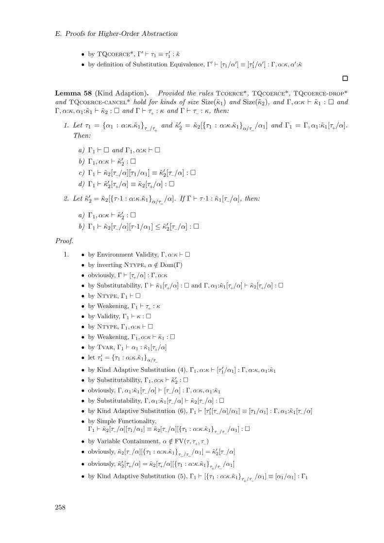
E. Proofs for Higher-Order Abstraction
• by TQcoerce*, Γ′ ⊢ τ1 ≡ τ ′1 : κ
• by definition of Substitution Equivalence, Γ′ ⊢ [τ1/α′] ≡ [τ ′1/α
′] : Γ, α:κ, α′:κ
Lemma 58 (Kind Adaption). Provided the rules Tcoerce*, TQcoerce*, TQcoerce-drop*
and TQcoerce-cancel* hold for kinds of size Size(κ1) and Size(κ2), and Γ, α:κ ⊢ κ1 : andΓ, α:κ, α1:κ1 ⊢ κ2 : and Γ ⊢ τ
+: κ and Γ ⊢ τ− : κ, then:
1. Let τ1 = α1 : α:κ.κ1τ−/τ+
and κ′2 = κ2[τ1 : α:κ.κ1α/τ−/α1] and Γ1 = Γ, α1:κ1[τ+/α].
Then:
a) Γ1 ⊢ and Γ1, α:κ ⊢
b) Γ1, α:κ ⊢ κ′2 :
c) Γ1 ⊢ κ2[τ−/α][τ1/α1] ≡ κ′2[τ−/α] :
d) Γ1 ⊢ κ′2[τ+/α] ≡ κ2[τ+/α] :
2. Let κ′2 = κ2[τ ·1 : α:κ.κ1α/τ−/α]. If Γ ⊢ τ ·1 : κ1[τ−/α], then:
a) Γ1, α:κ ⊢ κ′2 :
b) Γ1 ⊢ κ2[τ−/α][τ ·1/α1] ≤ κ′2[τ−/α] :
Proof.
1. • by Environment Validity, Γ, α:κ ⊢
• by inverting Ntype, α /∈ Dom(Γ)
• obviously, Γ ⊢ [τ+/α] : Γ, α:κ
• by Substitutability, Γ ⊢ κ1[τ+/α] : and Γ, α1:κ1[τ+/α] ⊢ κ2[τ+/α] :
• by Ntype, Γ1 ⊢
• by Weakening, Γ1 ⊢ τ+
: κ
• by Validity, Γ1 ⊢ κ :
• by Ntype, Γ1, α:κ ⊢
• by Weakening, Γ1, α:κ ⊢ κ1 :
• by Tvar, Γ1 ⊢ α1 : κ1[τ+/α]
• let τ ′1 = τ1 : α:κ.κ1α/τ−
• by Kind Adaptive Substitution (4), Γ1, α:κ ⊢ [τ ′1/α1] : Γ, α:κ, α1:κ1
• by Substitutability, Γ1, α:κ ⊢ κ′2 :
• obviously, Γ, α1:κ1[τ−/α] ⊢ [τ−/α] : Γ, α:κ, α1:κ1
• by Substitutability, Γ, α1:κ1[τ−/α] ⊢ κ2[τ−/α] :
• by Kind Adaptive Substitution (6), Γ1 ⊢ [τ ′1[τ−/α]/α1] ≡ [τ1/α1] : Γ, α1:κ1[τ−/α]
• by Simple Functionality,Γ1 ⊢ κ2[τ−/α][τ1/α1] ≡ κ2[τ−/α][τ1 : α:κ.κ1τ
−/τ
−/α1] :
• by Variable Containment, α /∈ FV(τ, τ+, τ−)
• obviously, κ2[τ−/α][τ1 : α:κ.κ1τ−/τ−/α1] = κ′2[τ−/α]
• obviously, κ′2[τ+/α] = κ2[τ+/α][τ1 : α:κ.κ1τ+
/τ−/α1]
• by Kind Adaptive Substitution (5), Γ1 ⊢ [τ1 : α:κ.κ1τ+
/τ−/α1] ≡ [α1/α1] : Γ1
258
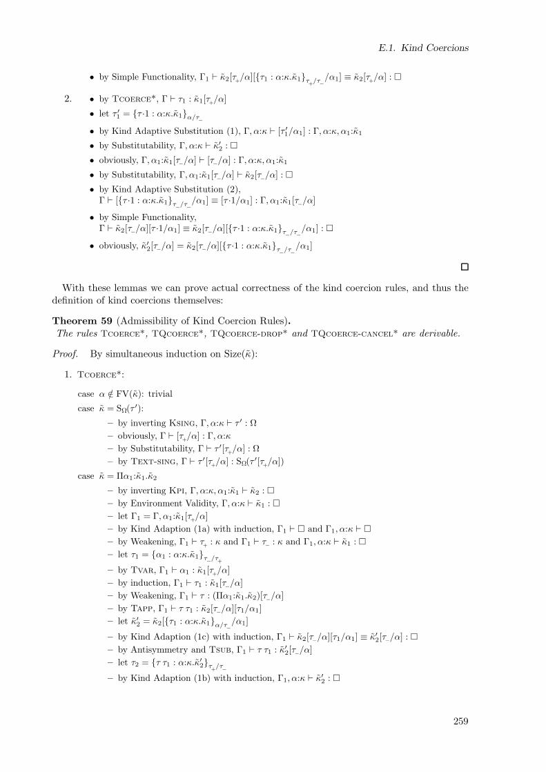
E.1. Kind Coercions
• by Simple Functionality, Γ1 ⊢ κ2[τ+/α][τ1 : α:κ.κ1τ+
/τ−/α1] ≡ κ2[τ+/α] :
2. • by Tcoerce*, Γ ⊢ τ1 : κ1[τ+/α]
• let τ ′1 = τ ·1 : α:κ.κ1α/τ−
• by Kind Adaptive Substitution (1), Γ, α:κ ⊢ [τ ′1/α1] : Γ, α:κ, α1:κ1
• by Substitutability, Γ, α:κ ⊢ κ′2 :
• obviously, Γ, α1:κ1[τ−/α] ⊢ [τ−/α] : Γ, α:κ, α1:κ1
• by Substitutability, Γ, α1:κ1[τ−/α] ⊢ κ2[τ−/α] :
• by Kind Adaptive Substitution (2),Γ ⊢ [τ ·1 : α:κ.κ1τ−/τ−
/α1] ≡ [τ ·1/α1] : Γ, α1:κ1[τ−/α]
• by Simple Functionality,Γ ⊢ κ2[τ−/α][τ ·1/α1] ≡ κ2[τ−/α][τ ·1 : α:κ.κ1τ
−/τ
−/α1] :
• obviously, κ′2[τ−/α] = κ2[τ−/α][τ ·1 : α:κ.κ1τ−
/τ−/α1]
With these lemmas we can prove actual correctness of the kind coercion rules, and thus thedefinition of kind coercions themselves:
Theorem 59 (Admissibility of Kind Coercion Rules).The rules Tcoerce*, TQcoerce*, TQcoerce-drop* and TQcoerce-cancel* are derivable.
Proof. By simultaneous induction on Size(κ):
1. Tcoerce*:
case α /∈ FV(κ): trivial
case κ = SΩ(τ ′):
– by inverting Ksing, Γ, α:κ ⊢ τ ′ : Ω
– obviously, Γ ⊢ [τ+/α] : Γ, α:κ
– by Substitutability, Γ ⊢ τ ′[τ+/α] : Ω
– by Text-sing, Γ ⊢ τ ′[τ+/α] : SΩ(τ ′[τ
+/α])
case κ = Πα1:κ1.κ2
– by inverting Kpi, Γ, α:κ, α1:κ1 ⊢ κ2 :
– by Environment Validity, Γ, α:κ ⊢ κ1 :
– let Γ1 = Γ, α1:κ1[τ+/α]
– by Kind Adaption (1a) with induction, Γ1 ⊢ and Γ1, α:κ ⊢
– by Weakening, Γ1 ⊢ τ+ : κ and Γ1 ⊢ τ− : κ and Γ1, α:κ ⊢ κ1 :
– let τ1 = α1 : α:κ.κ1τ−
/τ+
– by Tvar, Γ1 ⊢ α1 : κ1[τ+/α]
– by induction, Γ1 ⊢ τ1 : κ1[τ−/α]
– by Weakening, Γ1 ⊢ τ : (Πα1:κ1.κ2)[τ−/α]
– by Tapp, Γ1 ⊢ τ τ1 : κ2[τ−/α][τ1/α1]
– let κ′2 = κ2[τ1 : α:κ.κ1α/τ−/α1]
– by Kind Adaption (1c) with induction, Γ1 ⊢ κ2[τ−/α][τ1/α1] ≡ κ′2[τ−/α] :
– by Antisymmetry and Tsub, Γ1 ⊢ τ τ1 : κ′2[τ−/α]
– let τ2 = τ τ1 : α:κ.κ′2τ+
/τ−
– by Kind Adaption (1b) with induction, Γ1, α:κ ⊢ κ′2 :
259
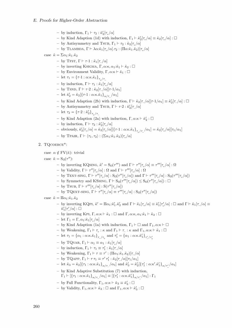
E. Proofs for Higher-Order Abstraction
– by induction, Γ1 ⊢ τ2 : κ′2[τ+/α]
– by Kind Adaption (1d) with induction, Γ1 ⊢ κ′2[τ+/α] ≡ κ2[τ+/α] :
– by Antisymmetry and Tsub, Γ1 ⊢ τ2 : κ2[τ+/α]
– by Tlambda, Γ ⊢ λα:κ1[τ+/α].τ2 : (Πα:κ1.κ2)[τ+/α]
case κ = Σα1:κ1.κ2
– by Tfst, Γ ⊢ τ ·1 : κ1[τ−/α]
– by inverting Ksigma, Γ, α:κ, α1:κ1 ⊢ κ2 :
– by Environment Validity, Γ, α:κ ⊢ κ1 :
– let τ1 = τ ·1 : α:κ.κ1τ+
/τ−
– by induction, Γ ⊢ τ1 : κ1[τ+/α]
– by Tsnd, Γ ⊢ τ ·2 : κ2[τ−/α][τ ·1/α1]
– let κ′2 = κ2[τ ·1 : α:κ.κ1α/τ−/α1]
– by Kind Adaption (2b) with induction, Γ ⊢ κ2[τ−/α][τ ·1/α1] ≡ κ′2[τ−/α] :
– by Antisymmetry and Tsub, Γ ⊢ τ ·2 : κ′2[τ−/α]
– let τ2 = τ ·2 : κ′2τ+
/τ−
– by Kind Adaption (2a) with induction, Γ, α:κ ⊢ κ′2 :
– by induction, Γ ⊢ τ2 : κ′2[τ+/α]
– obviously, κ′2[τ+/α] = κ2[τ+/α][τ ·1 : α:κ.κ1τ+
/τ−/α1] = κ2[τ+/α][τ1/α1]
– by Tpair, Γ ⊢ 〈τ1, τ2〉 : (Σα1:κ1.κ2)[τ+/α]
2. TQcoerce*:
case α /∈ FV(κ): trivial
case κ = SΩ(τ ′′):
– by inverting KQsing, κ′ = SΩ(τ ′′′) and Γ ⊢ τ ′′[τ+/α] ≡ τ ′′′[τ
+/α] : Ω
– by Validity, Γ ⊢ τ ′′[τ+/α] : Ω and Γ ⊢ τ ′′′[τ
+/α] : Ω
– by Text-sing, Γ ⊢ τ ′′[τ+/α] : SΩ(τ ′′[τ
+/α]) and Γ ⊢ τ ′′′[τ
+/α] : SΩ(τ ′′′[τ
+/α])
– by Symmetry and KSsing, Γ ⊢ SΩ(τ ′′′[τ+/α]) ≤ SΩ(τ ′′[τ
+/α]) :
– by Tsub, Γ ⊢ τ ′′′[τ+/α] : S(τ ′′[τ
+/α])
– by TQext-sing, Γ ⊢ τ ′′[τ+/α] ≡ τ ′′′[τ
+/α] : SΩ(τ ′′[τ
+/α])
case κ = Πα1:κ1.κ2
– by inverting KQpi, κ′ = Πα1:κ′1.κ
′2 and Γ ⊢ κ1[τ+/α] ≡ κ′1[τ
′+/α] : and Γ ⊢ κ1[τ−/α] ≡
κ′1[τ′−/α] :
– by inverting Kpi, Γ, α:κ ⊢ κ1 : and Γ, α:κ, α1:κ1 ⊢ κ2 :
– let Γ1 = Γ, α1:κ1[τ+/α]
– by Kind Adaption (1a) with induction, Γ1 ⊢ and Γ1, α:κ ⊢
– by Weakening, Γ1 ⊢ τ+
: κ and Γ1 ⊢ τ− : κ and Γ1, α:κ ⊢ κ1 :
– let τ1 = α1 : α:κ.κ1τ−
/τ+
and τ ′1 = α1 : α:κ.κ′1τ ′−
/τ ′+
– by TQvar, Γ1 ⊢ α1 ≡ α1 : κ1[τ+/α]
– by induction, Γ1 ⊢ τ1 ≡ τ ′1 : κ1[τ−/α]
– by Weakening, Γ1 ⊢ τ ≡ τ ′ : (Πα1:κ1.κ2)[τ−/α]
– by TQapp, Γ1 ⊢ τ τ1 ≡ τ ′ τ ′1 : κ2[τ−/α][τ1/α1]
– let κ3 = κ2[τ1 : α:κ.κ1α/τ−/α1] and κ′3 = κ′2[τ
′1 : α:κ′.κ′1α/τ ′
−
/α1]
– by Kind Adaptive Substitution (7) with induction,Γ1 ⊢ [τ1 : α:κ.κ1α/τ
−/α1] ≡ [τ ′1 : α:κ.κ′1α/τ ′
−
/α1] : Γ1
– by Full Functionality, Γ1, α:κ ⊢ κ3 ≡ κ′3 :
– by Validity, Γ1, α:κ ⊢ κ3 : and Γ1, α:κ ⊢ κ′3 :
260
E.1. Kind Coercions
– obviously, Γ1 ⊢ [τ+/α] ≡ [τ ′
+/α] : Γ1, α:κ and Γ1 ⊢ [τ−/α] ≡ [τ ′
−/α] : Γ1, α:κ
– by Full Functionality, Γ1 ⊢ κ3[τ+/α] ≡ κ′3[τ′+/α] : and Γ1 ⊢ κ3[τ−/α] ≡ κ′3[τ
′−/α] :
– by Kind Adaption (1c) with induction, Γ1 ⊢ κ2[τ−/α][τ1/α1] ≡ κ3[τ−/α] :
– by Antisymmetry and TQsub, Γ1 ⊢ τ τ1 ≡ τ ′ τ ′1 : κ3[τ−/α]
– let τ2 = τ τ1 : α:κ.κ3τ+
/τ−
and τ ′2 = τ ′ τ ′1 : α:κ′.κ′3τ+
/τ−
– by Kind Adaption (1b) with induction, Γ1, α:κ ⊢ κ3 : and Γ1, α:κ ⊢ κ′3 :
– by induction, Γ1 ⊢ τ2 ≡ τ ′2 : κ3[τ+/α]
– by Kind Adaption (1d) with induction, Γ1 ⊢ κ3[τ+/α] ≡ κ2[τ+/α] :
– by Antisymmetry and TQsub, Γ1 ⊢ τ2 ≡ τ ′2 : κ2[τ+/α]
– by TQlambda, Γ ⊢ λα:κ1[τ+/α].τ2 ≡ λα:κ′1[τ′+/α].τ ′2 : (Πα:κ1.κ2)[τ+/α]
case κ = Σα1:κ1.κ2
– by inverting KQsigma, κ′ = Σα1:κ′1.κ
′2 and Γ ⊢ κ1[τ+/α] ≡ κ′1[τ
′+/α] : and Γ ⊢
κ1[τ−/α] ≡ κ′1[τ′−/α] :
– by TQfst, Γ ⊢ τ ·1 ≡ τ ′·1 : κ1[τ−/α]
– by inverting Ksigma, Γ, α:κ ⊢ κ1 : and Γ, α:κ, α1:κ1 ⊢ κ2 :
– let τ1 = τ ·1 : α:κ.κ1τ+
/τ−and τ ′1 = τ ′·1 : α:κ′.κ′1τ ′
+/τ ′
−
– by induction, Γ ⊢ τ1 ≡ τ ′1 : κ1[τ+/α]
– by TQsnd, Γ ⊢ τ ·2 ≡ τ ′·2 : κ2[τ−/α][τ ·1/α1]
– let κ3 = κ2[τ ·1 : α:κ.κ1α/τ−/α1] and κ′3 = κ′2[τ
′·1 : α:κ′.κ′1α/τ ′−
/α1]
– by Kind Adaptive Substitution (3) with induction,Γ1 ⊢ [τ ·1 : α:κ.κ1α/τ−
/α1] ≡ [τ ′·1 : α:κ′.κ′1α/τ ′−
/α1] : Γ1
– by Full Functionality, Γ1 ⊢ κ3 ≡ κ′3 :
– by Validity, Γ, α:κ ⊢ κ3 : and Γ, α:κ ⊢ κ′3 :
– obviously, Γ ⊢ [τ+/α] ≡ [τ ′
+/α] : Γ, α:κ and Γ ⊢ [τ−/α] ≡ [τ ′
−/α] : Γ, α:κ
– by Full Functionality, Γ ⊢ κ3[τ+/α] ≡ κ′3[τ′+/α] : and Γ ⊢ κ3[τ−/α] ≡ κ′3[τ
′−/α] :
– by Kind Adaption (2b) with induction, Γ ⊢ κ2[τ−/α][τ ·1/α1] ≡ κ3[τ−/α] :
– by Antisymmetry and TQsub, Γ ⊢ τ ·2 ≡ τ ′·2 : κ′2[τ−/α]
– let τ2 = τ ·2 : α:κ.κ3τ+
/τ−and τ ′2 = τ ′·2 : α:κ′.κ′3τ ′
+/τ ′
−
– by induction, Γ ⊢ τ2 ≡ τ ′2 : κ3[τ+/α]
– obviously, κ3[τ+/α] = κ2[τ+/α][τ ·1 : α:κ.κ1τ+
/τ−/α1] = κ2[τ+/α][τ1/α1]
– by TQpair, Γ ⊢ 〈τ1, τ2〉 ≡ 〈τ ′1, τ′2〉 : (Σα1:κ1.κ2)[τ+/α]
3. TQcoerce-drop*:
case α /∈ FV(κ):
– by Reflexivity, Γ ⊢ τ ≡ τ : κ
case κ = SΩ(τ ′):
– by Validity, Γ ⊢ τ+
: κ and Γ ⊢ τ− : κ
– by Tcoerce*, Γ ⊢ τ : α:κ.SΩ(τ ′)τ+
/τ−
: SΩ(τ ′)[τ+/α]
– by Environment Validity, Γ ⊢
– obviously, Γ ⊢ [τ+/α] ≡ [τ−/α] : Γ, α:κ
– by Simple Functionality, Γ ⊢ SΩ(τ ′)[τ+/α] ≤ SΩ(τ ′)[τ−/α] :
– by Tsub, Γ ⊢ τ : α:κ.SΩ(τ ′)τ+
/τ−: SΩ(τ ′)[τ−/α]
– by TQext-sing, Γ ⊢ τ : α:κ.SΩ(τ ′)τ+
/τ−≡ τ : SΩ(τ ′)[τ−/α]
case κ = Πα1:κ1.κ2
– by Validity, Γ ⊢ τ+
: κ and Γ ⊢ τ− : κ
261
E. Proofs for Higher-Order Abstraction
– by inverting Kpi, Γ, α:κ, α1:κ1 ⊢ κ2 :
– by Environment Validity, Γ, α:κ ⊢ κ1 :
– let Γ1 = Γ, α1:κ1[τ+/α]
– by Kind Adaption (1a) with induction, Γ1 ⊢ and Γ1, α:κ ⊢
– by Weakening, Γ1 ⊢ τ+≡ τ− : κ and Γ1, α:κ ⊢ κ1 :
– by Symmetry, Γ1 ⊢ τ− ≡ τ+
: κ
– let τ1 = α1 : α:κ.κ1τ−
/τ+
– by Tvar, Γ1 ⊢ α1 : κ1[τ+/α]
– by induction, Γ1 ⊢ τ1 ≡ α1 : κ1[τ+/α]
– obviously, Γ1 ⊢ [τ+/α] ≡ [τ−/α] : Γ1, α:κ
– by Simple Functionality, Γ1 ⊢ κ1[τ+/α] ≤ κ1[τ−/α] :
– by TQsub, Γ1 ⊢ τ1 ≡ α1 : κ1[τ−/α]
– by Weakening, Γ1 ⊢ τ : (Πα1:κ1.κ2)[τ−/α]
– by Reflexivity, Γ1 ⊢ τ ≡ τ : Πα1:κ1[τ−/α].κ2[τ−/α]
– by TQapp, Γ1 ⊢ τ τ1 ≡ τ α1 : κ2[τ−/α][τ1/α1]
– let κ′2 = κ2[τ1 : α:κ.κ1α/τ−/α1]
– by Kind Adaption (1c) with induction, Γ1 ⊢ κ2[τ−/α][τ1/α1] ≡ κ′2[τ−/α] :
– by Antisymmetry and TQsub, Γ1 ⊢ τ τ1 ≡ τ α1 : κ′2[τ−/α]
– let τ2 = τ τ1 : α:κ.κ′2τ+≈τ
−and τ ′2 = τ α1 : α:κ.κ′2τ
+≈τ
−
– by Validity, Γ1 ⊢ τ τ1 : κ′2[τ−/α] and Γ1 ⊢ τ α1 : κ′2[τ−/α]
– by Kind Adaption (1b) with induction, Γ1, α:κ ⊢ κ′2 :
– by induction, Γ1 ⊢ τ2 ≡ τ τ1 : κ′2[τ−/α] and Γ1 ⊢ τ ′2 ≡ τ α1 : κ′2[τ−/α]
– by Symmetry and Transitivity, Γ1 ⊢ τ2 ≡ τ α1 : κ′2[τ−/α]
– by Simple Functionality, Γ1 ⊢ κ′2[τ−/α] ≤ κ′2[τ+/α] :
– by TQsub, Γ1 ⊢ τ2 ≡ τ α1 : κ′2[τ+/α]
– by Kind Adaption (1d) with induction, Γ1 ⊢ κ′2[τ+/α] ≡ κ2[τ+/α] :
– by Antisymmetry and TQsub, Γ1 ⊢ τ2 ≡ τ α1 : κ2[τ+/α]
– by TQlambda, Γ ⊢ λα:κ1[τ+/α].τ2 ≡ λα:κ1[τ+/α].τ α1 : (Πα:κ1.κ2)[τ+/α]
– by Simple Functionality, Γ ⊢ (Πα:κ1.κ2)[τ+/α] ≤ (Πα:κ1.κ2)[τ−/α] :
– by TQsub, Γ ⊢ λα:κ1[τ+/α].τ2 ≡ λα:κ1[τ+/α].τ α1 : (Πα:κ1.κ2)[τ−/α]
– by TQlambda-eta*, Γ ⊢ λα:κ1[τ+/α].τ α1 ≡ τ : (Πα:κ1.κ2)[τ−/α]
– by Transitivity, Γ ⊢ λα:κ1[τ+/α].τ2 ≡ τ : (Πα:κ1.κ2)[τ−/α]
case κ = Σα1:κ1.κ2
– by Validity, Γ ⊢ τ+
: κ and Γ ⊢ τ− : κ
– obviously, Γ ⊢ [τ+/α] ≡ [τ−/α] : Γ, α:κ
– by Tfst, Γ ⊢ τ ·1 : κ1[τ−/α]
– by inverting Ksigma, Γ, α:κ, α1:κ1 ⊢ κ2 :
– by Environment Validity, Γ, α:κ ⊢ κ1 :
– let τ1 = τ ·1 : α:κ.κ1τ+
/τ−
– by induction, Γ ⊢ τ1 ≡ τ ·1 : κ1[τ−/α]
– by Validity, Γ ⊢ τ1 : κ1[τ−/α]
– by Tsnd, Γ ⊢ τ ·2 : κ2[τ−/α][τ ·1/α1]
– let κ′2 = κ2[τ ·1 : α:κ.κ1α/τ−/α1]
– by Kind Adaption (2b) with induction, Γ ⊢ κ2[τ−/α][τ ·1/α1] ≡ κ′2[τ−/α] :
– by Antisymmetry and Tsub, Γ ⊢ τ ·2 : κ′2[τ−/α]
– let τ2 = τ ·2 : κ′2τ+
/τ−
262
E.1. Kind Coercions
– by Kind Adaption (2a) with induction, Γ, α:κ ⊢ κ′2 :
– by induction, Γ ⊢ τ2 ≡ τ ·2 : κ′2[τ−/α]
– by Substitutability, Γ ⊢ κ′2[τ−/α] ≤ κ′2[τ+/α] :
– obviously, κ′2[τ+/α] = κ2[τ+/α][τ ·1 : α:κ.κ1τ+
/τ−/α1] = κ2[τ+/α][τ1/α1]
– obviously, Γ, α1:κ1[τ−/α] ⊢ [τ−/α] ≡ κ2[τ+/α] : Γ, α:κ, α:κ1
– by Simple Functionality, Γ, α1:κ1[τ−/α] ⊢ κ2[τ+/α] ≤ κ2[τ−/α] :
– obviously, Γ ⊢ [τ1/α1] : Γ, α1:κ1[τ−/α]
– by Substitutability, Γ ⊢ κ2[τ+/α][τ1/α1] ≤ κ2[τ−/α][τ1/α1] :
– by Transitivity, Γ ⊢ κ′2[τ−/α] ≤ κ2[τ−/α][τ1/α1] :
– TQsub, Γ ⊢ τ2 ≡ τ ·2 : κ2[τ−/α][τ1/α1]
– by TQpair, Γ ⊢ 〈τ1, τ2〉 ≡ 〈τ ·1, τ ·2〉 : (Σα1:κ1.κ2)[τ−/α]
– by TQpair-eta*, Γ ⊢ 〈τ ·1, τ ·2〉 ≡ τ : (Σα1:κ1.κ2)[τ−/α]
– by Transitivity, Γ ⊢ 〈τ1, τ2〉 ≡ τ : (Σα1:κ1.κ2)[τ−/α]
4. TQcoerce-cancel*:
case α /∈ FV(κ):
– by Reflexivity, Γ ⊢ τ ≡ τ : κ
case κ = SΩ(τ ′):
– by Validity, Γ ⊢ SΩ(τ ′)[τ−/α] :
– by inverting Ksing, Γ ⊢ τ ′[τ−/α] : Ω
– by Text-sing, Γ ⊢ τ ′[τ−/α] : SΩ(τ ′)[τ−/α]
– by TQext-sing, Γ ⊢ τ ′[τ−/α] ≡ τ : SΩ(τ ′)[τ−/α]
case κ = Σα1:κ1.κ2
– let τ1 = τ ·1 : α:κ.κ1τ+
/τ−
and τ2 = τ ·2 : κ′2τ+
/τ−
and τ ′ = 〈τ1, τ2〉
with κ′2 = κ2[τ ·1 : α:κ.κ1α/τ−/α1] and
– let τ ′1 = τ ′·1 : α:κ.κ1τ−
/τ+
and τ ′2 = τ ′·2 : κ′′2τ−
/τ+
and τ ′′ = 〈τ ′1, τ′2〉
with κ′′2 = κ2[τ ′·1 : α:κ.κ1α/τ+/α1]
– by Tcoerce*, Γ ⊢ τ ′ : (Σα1:κ1.κ2)[τ+/α]
– by TQfst-beta*, Γ ⊢ τ ′·1 ≡ τ1 : κ1[τ+/α]
– by TQsnd-beta*, Γ ⊢ τ ′·2 ≡ τ2 : κ2[τ+/α][τ ′·1/α1]
– by inverting Ksigma, Γ, α:κ, α1:κ1 ⊢ κ2 :
– by Environment Validity, Γ, α:κ ⊢ κ1 :
– obviously, Γ ⊢ [τ+/α] : Γ, α:κ and Γ ⊢ [τ−/α] : Γ, α:κ
– by Substitutability, Γ ⊢ κ1[τ+/α] : and Γ ⊢ κ1[τ−/α] :
– by Reflexivity, Γ ⊢ κ1[τ+/α] ≡ κ1[τ+/α] : and Γ ⊢ κ1[τ−/α] ≡ κ1[τ−/α] : andΓ ⊢ τ
+≡ τ
+: κ and Γ ⊢ τ− ≡ τ− : κ
– by TQcoerce*, Γ ⊢ τ ′1 ≡ τ1 : α:κ.κ1τ−
/τ+
: κ1[τ−/α]
– by Tfst, Γ ⊢ τ ·1 : κ1[τ−/α]
– by induction, Γ ⊢ τ1 : α:κ.κ1τ−/τ+≡ τ ·1 : κ1[τ−/α]
– by Transitivity, Γ ⊢ τ ′1 ≡ τ ·1 : κ1[τ−/α]
– by Validity, Γ ⊢ τ ′·1 : κ1[τ+/α]
– by Kind Adaption (2b) with induction (inverted signs),Γ ⊢ κ2[τ+/α][τ ′·1/α1] ≡ κ′′2 [τ
+/α] :
– by Antisymmetry and TQsub, Γ ⊢ τ ′·2 ≡ τ2 : κ′′2 [τ+/α]
– by Kind Adaption (2a) with induction (inverted signs), Γ, α:κ ⊢ κ′′2 :
– by Substitutability, Γ ⊢ κ′′2 [τ+/α] : and Γ ⊢ κ′′2 [τ−/α] :
263
E. Proofs for Higher-Order Abstraction
– by Reflexivity, Γ ⊢ κ′′2 [τ+/α] ≡ κ′′2 [τ
+/α] : and Γ ⊢ κ′′2 [τ−/α] ≡ κ′′2 [τ−/α] :
– by TQcoerce*, Γ ⊢ τ ′2 ≡ τ2 : α:κ.κ′′2τ−
/τ+
: κ′′2 [τ−/α]
– obviously, κ′2[τ+/α] = κ2[τ+/α][τ1/α1]and κ′′2 [τ
+/α] = κ2[τ+/α][τ ′·1 : α:κ.κ1τ
+/τ
+/α1]
– obviously, Γ, α1:κ1[τ+/α] ⊢ [τ+/α] : Γ, α:κ, α1:κ1
– by Substitutability, Γ, α1:κ1[τ+/α] ⊢ κ2[τ+/α] :
– by TQcoerce-drop*, Γ ⊢ τ ′·1 : α:κ.κ1τ+
/τ+≡ τ ′·1 : κ1[τ+/α] :
– by Transitivity, Γ ⊢ τ ′·1 : α:κ.κ1τ+
/τ+≡ τ1 : κ1[τ+/α] :
– obviously, Γ ⊢ [τ ′·1 : α:κ.κ1τ+
/τ+/α1] ≡ [τ1/α1] : Γ, α1:κ1[τ+/α]
– by Simple Functionality, Γ ⊢ κ′2[τ+/α] ≡ κ′′2 [τ+/α] :
– obviously, κ′2[τ−/α] = κ2[τ−/α][τ ·1 : α:κ.κ1τ−/τ−/α1]
and κ′′2 [τ−/α] = κ2[τ−/α][τ ′·1 : α:κ.κ1τ−/τ+/α1]
– by TQcoerce-drop*, Γ ⊢ τ ·1 : α:κ.κ1τ−
/τ−≡ τ ·1 : κ1[τ−/α] :
– by TQcoerce*, Γ ⊢ τ ′·1 : α:κ.κ1τ−
/τ+≡ τ1 : α:κ.κ1τ
−/τ
+: κ1[τ−/α] :
– by induction, Γ ⊢ τ1 : α:κ.κ1τ−/τ+≡ τ ·1 : κ1[τ−/α] :
– by Symmetry and Transitivity,Γ ⊢ τ ·1 : α:κ.κ1τ
−/τ
−≡ τ ′·1 : α:κ.κ1τ
−/τ
+: κ1[τ−/α] :
– obviously, Γ ⊢ [τ ·1 : α:κ.κ1τ−
/τ−
+/α1] ≡ [τ ′·1 : α:κ.κ1τ−
/τ+/α1] : Γ, α1:κ1[τ+/α]
– by Simple Functionality, Γ ⊢ κ′2[τ−/α] ≡ κ′′2 [τ−/α] :
– by Tsnd, Γ ⊢ τ ·2 : κ2[τ−/α][τ ·1/α1]
– by Kind Adaption (2b) with induction, Γ ⊢ κ2[τ−/α][τ ·1/α1] ≡ κ′2[τ−/α] :
– by Antisymmetry and Tsub, Γ ⊢ τ ·2 : κ′2[τ−/α]
– by induction, Γ ⊢ τ2 : κ′2τ−
/τ+≡ τ ·2 : κ′2[τ−/α]
– by Tcoerce*, Γ ⊢ τ2 : κ′2[τ+/α]
– by Reflexivity, Γ ⊢ τ2 ≡ τ2 : κ′2[τ+/α]
– by TQcoerce*, Γ ⊢ τ2 : α:κ.κ′2τ−/τ+≡ τ ′2 : κ′2[τ−/α]
– by Symmetry and Transitivity, Γ ⊢ τ ′2 ≡ τ ·2 : κ′2[τ−/α]
– by Antisymmetry and TQsub, Γ ⊢ τ ′2 ≡ τ ·2 : κ2[τ−/α][τ ·1/α1]
– by Symmetry, Γ ⊢ τ ·1 ≡ τ ′1 : κ1[τ−/α] and Γ ⊢ τ ·2 ≡ τ ′2 : κ2[τ−/α][τ ·1/α1]
– by TQpair, Γ ⊢ 〈τ ·1, τ ·2〉 ≡ τ ′′ : (Σα1:κ1.κ2)[τ−/α]
– by TQpair-eta*, Γ ⊢ 〈τ ·1, τ ·2〉 ≡ τ : (Σα1:κ1.κ2)[τ−/α]
– by Symmetry and Transitivity, Γ ⊢ τ ′′ ≡ τ : (Σα1:κ1.κ2)[τ−/α]
E.2. Abstraction Kinds
The definition of higher-order abstraction kinds mostly follows higher-order singleton kinds, sothe proofs of admissibility are similar as well. However, to deal with the coercion in the Σ-casewe state a technical lemma:
Lemma 60 (Second Component Conversion).
1. If Γ ⊢ τ : Σα1:κ1.κ2, then Γ, α1:κ1 ⊢ τ ·2 : α1:κ1.κ2α1/τ ·1 : κ2.
264
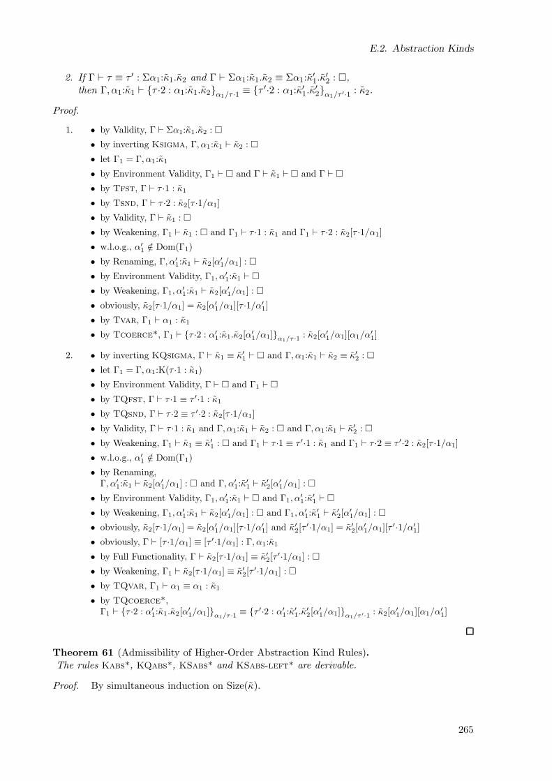
E.2. Abstraction Kinds
2. If Γ ⊢ τ ≡ τ ′ : Σα1:κ1.κ2 and Γ ⊢ Σα1:κ1.κ2 ≡ Σα1:κ′1.κ
′2 : ,
then Γ, α1:κ1 ⊢ τ ·2 : α1:κ1.κ2α1/τ ·1 ≡ τ ′·2 : α1:κ′1.κ
′2α1/τ ′·1 : κ2.
Proof.
1. • by Validity, Γ ⊢ Σα1:κ1.κ2 :
• by inverting Ksigma, Γ, α1:κ1 ⊢ κ2 :
• let Γ1 = Γ, α1:κ1
• by Environment Validity, Γ1 ⊢ and Γ ⊢ κ1 ⊢ and Γ ⊢
• by Tfst, Γ ⊢ τ ·1 : κ1
• by Tsnd, Γ ⊢ τ ·2 : κ2[τ ·1/α1]
• by Validity, Γ ⊢ κ1 :
• by Weakening, Γ1 ⊢ κ1 : and Γ1 ⊢ τ ·1 : κ1 and Γ1 ⊢ τ ·2 : κ2[τ ·1/α1]
• w.l.o.g., α′1 /∈ Dom(Γ1)
• by Renaming, Γ, α′1:κ1 ⊢ κ2[α
′1/α1] :
• by Environment Validity, Γ1, α′1:κ1 ⊢
• by Weakening, Γ1, α′1:κ1 ⊢ κ2[α
′1/α1] :
• obviously, κ2[τ ·1/α1] = κ2[α′1/α1][τ ·1/α′
1]
• by Tvar, Γ1 ⊢ α1 : κ1
• by Tcoerce*, Γ1 ⊢ τ ·2 : α′1:κ1.κ2[α
′1/α1]α1/τ ·1 : κ2[α
′1/α1][α1/α
′1]
2. • by inverting KQsigma, Γ ⊢ κ1 ≡ κ′1 ⊢ and Γ, α1:κ1 ⊢ κ2 ≡ κ′2 :
• let Γ1 = Γ, α1:K(τ ·1 : κ1)
• by Environment Validity, Γ ⊢ and Γ1 ⊢
• by TQfst, Γ ⊢ τ ·1 ≡ τ ′·1 : κ1
• by TQsnd, Γ ⊢ τ ·2 ≡ τ ′·2 : κ2[τ ·1/α1]
• by Validity, Γ ⊢ τ ·1 : κ1 and Γ, α1:κ1 ⊢ κ2 : and Γ, α1:κ1 ⊢ κ′2 :
• by Weakening, Γ1 ⊢ κ1 ≡ κ′1 : and Γ1 ⊢ τ ·1 ≡ τ ′·1 : κ1 and Γ1 ⊢ τ ·2 ≡ τ ′·2 : κ2[τ ·1/α1]
• w.l.o.g., α′1 /∈ Dom(Γ1)
• by Renaming,Γ, α′
1:κ1 ⊢ κ2[α′1/α1] : and Γ, α′
1:κ′1 ⊢ κ′2[α
′1/α1] :
• by Environment Validity, Γ1, α′1:κ1 ⊢ and Γ1, α
′1:κ
′1 ⊢
• by Weakening, Γ1, α′1:κ1 ⊢ κ2[α
′1/α1] : and Γ1, α
′1:κ
′1 ⊢ κ′2[α
′1/α1] :
• obviously, κ2[τ ·1/α1] = κ2[α′1/α1][τ ·1/α′
1] and κ′2[τ′·1/α1] = κ′2[α
′1/α1][τ
′·1/α′1]
• obviously, Γ ⊢ [τ ·1/α1] ≡ [τ ′·1/α1] : Γ, α1:κ1
• by Full Functionality, Γ ⊢ κ2[τ ·1/α1] ≡ κ′2[τ′·1/α1] :
• by Weakening, Γ1 ⊢ κ2[τ ·1/α1] ≡ κ′2[τ′·1/α1] :
• by TQvar, Γ1 ⊢ α1 ≡ α1 : κ1
• by TQcoerce*,Γ1 ⊢ τ ·2 : α′
1:κ1.κ2[α′1/α1]α1/τ ·1 ≡ τ ′·2 : α′
1:κ′1.κ
′2[α
′1/α1]α1/τ ′·1 : κ2[α
′1/α1][α1/α
′1]
Theorem 61 (Admissibility of Higher-Order Abstraction Kind Rules).The rules Kabs*, KQabs*, KSabs* and KSabs-left* are derivable.
Proof. By simultaneous induction on Size(κ).
265
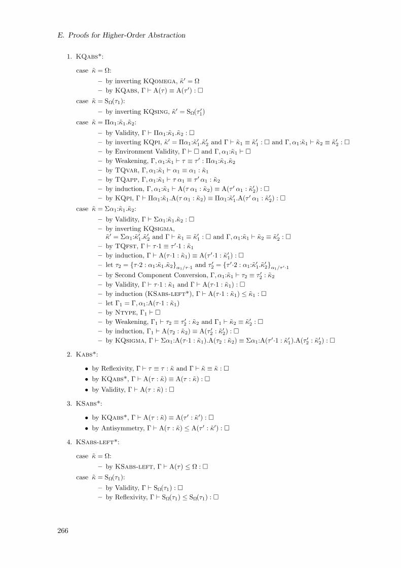
E. Proofs for Higher-Order Abstraction
1. KQabs*:
case κ = Ω:
– by inverting KQomega, κ′ = Ω
– by KQabs, Γ ⊢ A(τ) ≡ A(τ ′) :
case κ = SΩ(τ1):
– by inverting KQsing, κ′ = SΩ(τ ′1)
case κ = Πα1:κ1.κ2:
– by Validity, Γ ⊢ Πα1:κ1.κ2 :
– by inverting KQpi, κ′ = Πα1:κ′1.κ
′2 and Γ ⊢ κ1 ≡ κ′1 : and Γ, α1:κ1 ⊢ κ2 ≡ κ′2 :
– by Environment Validity, Γ ⊢ and Γ, α1:κ1 ⊢
– by Weakening, Γ, α1:κ1 ⊢ τ ≡ τ ′ : Πα1:κ1.κ2
– by TQvar, Γ, α1:κ1 ⊢ α1 ≡ α1 : κ1
– by TQapp, Γ, α1:κ1 ⊢ τ α1 ≡ τ ′ α1 : κ2
– by induction, Γ, α1:κ1 ⊢ A(τ α1 : κ2) ≡ A(τ ′ α1 : κ′2) :
– by KQpi, Γ ⊢ Πα1:κ1.A(τ α1 : κ2) ≡ Πα1:κ′1.A(τ ′ α1 : κ′2) :
case κ = Σα1:κ1.κ2:
– by Validity, Γ ⊢ Σα1:κ1.κ2 :
– by inverting KQsigma,κ′ = Σα1:κ
′1.κ
′2 and Γ ⊢ κ1 ≡ κ′1 : and Γ, α1:κ1 ⊢ κ2 ≡ κ′2 :
– by TQfst, Γ ⊢ τ ·1 ≡ τ ′·1 : κ1
– by induction, Γ ⊢ A(τ ·1 : κ1) ≡ A(τ ′·1 : κ′1) :
– let τ2 = τ ·2 : α1:κ1.κ2α1/τ ·1 and τ ′2 = τ ′·2 : α1:κ′1.κ
′2α1/τ ′·1
– by Second Component Conversion, Γ, α1:κ1 ⊢ τ2 ≡ τ ′2 : κ2
– by Validity, Γ ⊢ τ ·1 : κ1 and Γ ⊢ A(τ ·1 : κ1) :
– by induction (KSabs-left*), Γ ⊢ A(τ ·1 : κ1) ≤ κ1 :
– let Γ1 = Γ, α1:A(τ ·1 : κ1)
– by Ntype, Γ1 ⊢
– by Weakening, Γ1 ⊢ τ2 ≡ τ ′2 : κ2 and Γ1 ⊢ κ2 ≡ κ′2 :
– by induction, Γ1 ⊢ A(τ2 : κ2) ≡ A(τ ′2 : κ′2) :
– by KQsigma, Γ ⊢ Σα1:A(τ ·1 : κ1).A(τ2 : κ2) ≡ Σα1:A(τ ′·1 : κ′1).A(τ ′2 : κ′2) :
2. Kabs*:
• by Reflexivity, Γ ⊢ τ ≡ τ : κ and Γ ⊢ κ ≡ κ :
• by KQabs*, Γ ⊢ A(τ : κ) ≡ A(τ : κ) :
• by Validity, Γ ⊢ A(τ : κ) :
3. KSabs*:
• by KQabs*, Γ ⊢ A(τ : κ) ≡ A(τ ′ : κ′) :
• by Antisymmetry, Γ ⊢ A(τ : κ) ≤ A(τ ′ : κ′) :
4. KSabs-left*:
case κ = Ω:
– by KSabs-left, Γ ⊢ A(τ) ≤ Ω :
case κ = SΩ(τ1):
– by Validity, Γ ⊢ SΩ(τ1) :
– by Reflexivity, Γ ⊢ SΩ(τ1) ≤ SΩ(τ1) :
266
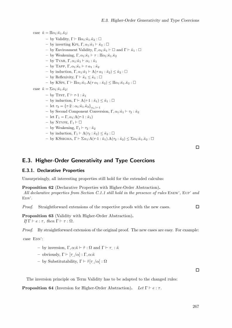
E.3. Higher-Order Generativity and Type Coercions
case κ = Πα1:κ1.κ2:
– by Validity, Γ ⊢ Πα1:κ1.κ2 :
– by inverting Kpi, Γ, α1:κ1 ⊢ κ2 :
– by Environment Validity, Γ, α1:κ1 ⊢ and Γ ⊢ κ1 :
– by Weakening, Γ, α1:κ1 ⊢ τ : Πα1:κ1.κ2
– by Tvar, Γ, α1:κ1 ⊢ α1 : κ1
– by Tapp, Γ, α1:κ1 ⊢ τ α1 : κ2
– by induction, Γ, α1:κ1 ⊢ A(τ α1 : κ2) ≤ κ2 :
– by Reflexivity, Γ ⊢ κ1 ≤ κ1 :
– by KSpi, Γ ⊢ Πα1:κ1.A(τ α1 : κ2) ≤ Πα1:κ1.κ2 :
case κ = Σα1:κ1.κ2:
– by Tfst, Γ ⊢ τ ·1 : κ1
– by induction, Γ ⊢ A(τ ·1 : κ1) ≤ κ1 :
– let τ2 = τ ·2 : α1:κ1.κ2α1/τ ·1
– by Second Component Conversion, Γ, α1:κ1 ⊢ τ2 : κ2
– let Γ1 = Γ, α1:A(τ ·1 : κ1)
– by Ntype, Γ1 ⊢
– by Weakening, Γ1 ⊢ τ2 : κ2
– by induction, Γ1 ⊢ A(τ2 : κ2) ≤ κ2 :
– by KSsigma, Γ ⊢ Σα1:A(τ ·1 : κ1).A(τ2 : κ2) ≤ Σα1:κ1.κ2 :
E.3. Higher-Order Generativity and Type Coercions
E.3.1. Declarative Properties
Unsurprisingly, all interesting properties still hold for the extended calculus:
Proposition 62 (Declarative Properties with Higher-Order Abstraction).All declarative properties from Section C.1.1 still hold in the presence of rules Enew’, Eup’ andEdn’.
Proof. Straightforward extensions of the respective proofs with the new cases.
Proposition 63 (Validity with Higher-Order Abstraction).If Γ ⊢ e : τ , then Γ ⊢ τ : Ω.
Proof. By straightforward extension of the original proof. The new cases are easy. For example:
case Edn’:
– by inversion, Γ, α:κ ⊢ τ : Ω and Γ ⊢ τ− : κ
– obviously, Γ ⊢ [τ−/α] : Γ, α:κ
– by Substitutability, Γ ⊢ τ [τ−/α] : Ω
The inversion principle on Term Validity has to be adapted to the changed rules:
Proposition 64 (Inversion for Higher-Order Abstraction). Let Γ ⊢ e : τ .
267
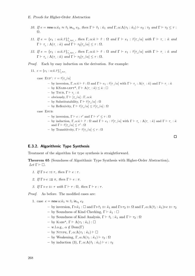
E. Proofs for Higher-Order Abstraction
10. If e = newα:κ1 ≈ τ1 inτ2 e2, then Γ ⊢ τ1 : κ1 and Γ, α:A(τ1 : κ1) ⊢ e2 : τ2 and Γ ⊢ τ2 ≤ τ :Ω.
11. If e = e1 : α:κ.τ+τ+≈τ−
, then Γ, α:κ ⊢ τ : Ω and Γ ⊢ e1 : τ [τ−/α] with Γ ⊢ τ− : κ and
Γ ⊢ τ+
: A(τ− : κ) and Γ ⊢ τ2[τ+/α] ≤ τ : Ω.
12. If e = e1 : α:κ.τ−τ+≈τ−
, then Γ, α:κ ⊢ τ : Ω and Γ ⊢ e1 : τ [τ+/α] with Γ ⊢ τ− : κ and
Γ ⊢ τ+
: A(τ− : κ) and Γ ⊢ τ2[τ−/α] ≤ τ : Ω.
Proof. Each by easy induction on the derivation. For example:
11. e = e1 : α:κ.τ+τ+≈τ
−
case Eup’: τ = τ [τ+/α]
– by inversion, Γ, α:κ ⊢ τ : Ω and Γ ⊢ e1 : τ [τ−/α] with Γ ⊢ τ+
: A(τ− : κ) and Γ ⊢ τ− : κ
– by KSabs-left*, Γ ⊢ A(τ− : κ) ≤ κ :
– by Tsub, Γ ⊢ τ+
: κ
– obviously, Γ ⊢ [τ+/α] : Γ, α:κ
– by Substitutability, Γ ⊢ τ [τ+/α] : Ω
– by Reflexivity, Γ ⊢ τ [τ+/α] ≤ τ [τ
+/α] : Ω
case Esub:
– by inversion, Γ ⊢ e : τ ′ and Γ ⊢ τ ′ ≤ τ : Ω
– by induction, Γ, α:κ ⊢ τ : Ω and Γ ⊢ e1 : τ [τ−/α] with Γ ⊢ τ+
: A(τ− : κ) and Γ ⊢ τ− : κand Γ ⊢ τ [τ
+/α] ≤ τ ′ : Ω
– by Transititvity, Γ ⊢ τ [τ+/α] ≤ τ : Ω
E.3.2. Algorithmic Type Synthesis
Treatment of the algorithm for type synthesis is straightforward.
Theorem 65 (Soundness of Algorithmic Type Synthesis with Higher-Order Abstraction).Let Γ ⊢ .
1. If Γ ⊲ e τ , then Γ ⊢ e : τ .
2. If Γ ⊲ e π, then Γ ⊢ e : π.
3. If Γ ⊲ e τ with Γ ⊢ τ : Ω, then Γ ⊢ e : τ .
Proof. As before. The modified cases are:
1. case e = newα:κ1 ≈ τ1 inτ2 e2
– by inversion, Γ⊲κ1 : and Γ⊲τ1 κ1 and Γ⊲τ2 Ω and Γ, α:A(τ1 : κ1)⊲e τ2
– by Soundness of Kind Checking, Γ ⊢ κ1 :
– by Soundness of Kind Analysis, Γ ⊢ τ1 : κ1 and Γ ⊢ τ2 : Ω
– by Kabs*, Γ ⊢ A(τ1 : κ1) :
– w.l.o.g., α /∈ Dom(Γ)
– by Ntype, Γ, α:A(τ1 : κ1) ⊢
– by Weakening, Γ, α:A(τ1 : κ1) ⊢ τ2 : Ω
– by induction (3), Γ, α:A(τ1 : κ1) ⊢ e : τ2
268
E.3. Higher-Order Generativity and Type Coercions
– by Enew’, Γ ⊢ (newα:κ1 ≈ τ1 inτ2 e2) : τ2
case e = e : α:κ.τ+τ+≈τ−
– by inversion, Γ ⊲ κ : and Γ ⊲ τ− κ and Γ ⊲ τ+ A(τ− : κ) and Γ, α:κ ⊲ τ Ω
and Γ ⊲ e τ [τ−/α]
– by Soundness of Kind Checking, Γ ⊢ κ :
– by Soundness of Kind Analysis, Γ ⊢ τ− : κ
– by Kabs*, Γ ⊢ A(τ− : κ) :
– by Soundness of Kind Analysis, Γ ⊢ τ+
: A(τ− : κ)
– w.l.o.g., α /∈ Dom(Γ)
– by Ntype, Γ, α:κ ⊢
– by Komega, Γ, α:κ ⊢ Ω :
– by Soundness of Kind Analysis, Γ, α:κ ⊢ τ : Ω
– obviously, Γ ⊢ [τ−/α] : Γ, α:κ
– by Substitutability, Γ ⊢ τ [τ−/α] : Ω
– by induction (3), Γ ⊢ e : τ [τ−/α]
– by Eup’, Γ ⊢ e : α:κ.τ+τ+≈τ−
: τ [τ+/α]
case e = e : α:κ.τ−τ+≈τ−
: analogous
Theorem 66 (Completeness of Algorithmic Type Synthesis with Higher-Order Abstraction).
1. If Γ ⊢ e : τ , then Γ ⊲ e τ ′ with Γ ⊢ τ ′ ≤ τ : Ω.
2. If Γ ⊢ e : τ , then Γ ⊲ e π with Γ ⊢ π ≤ τ : Ω.
3. If Γ ⊢ e : τ and Γ ⊢ τ ≤ τ ′ : Ω, then Γ ⊲ e τ ′.
Proof. As before. The modified cases are:
1. case Enew’:
– by inversion, Γ ⊢ τ1 : κ1 and Γ, α:A(τ1 : κ1) ⊢ e : τ2 and Γ ⊢ τ2 : Ω
– by Environment Validity, Γ ⊢ and Γ, α:A(τ1 : κ1) ⊢
– by Validity, Γ ⊢ κ1 : and Γ ⊢ Ω :
– by Completeness of Kind Checking, Γ ⊲ κ1 :
– by Completeness of Kind Analysis, Γ ⊲ τ1 κ1 and Γ ⊲ τ2 Ω
– by Weakening, Γ, α:A(τ1 : κ1) ⊢ τ2 : Ω
– by induction (3), Γ, α:A(τ1 : κ1) ⊲ e τ2
– by rule, Γ ⊲ (newα:κ1 ≈ τ1 inτ2 e2) τ2
case Eup’:
– by inversion, Γ ⊢ e : τ [τ−/α] and Γ, α:κ ⊢ τ : Ω and Γ ⊢ τ− : κ and Γ ⊢ τ+
: A(τ− :κ)
– by Environment Validity, Γ ⊢ and Γ, α:κ ⊢
– by Validity, Γ ⊢ τ [τ−/α] : and Γ, α:κ ⊢ Ω : and Γ ⊢ κ : and Γ ⊢ A(τ− : κ) :
– by Completeness of Kind Checking, Γ ⊲ κ :
269
E. Proofs for Higher-Order Abstraction
– by Completeness of Kind Analysis, Γ ⊲ τ− κ and Γ ⊲ τ+ A(τ− : κ) and
Γ, α:κ ⊲ τ Ω
– by induction (3), Γ ⊲ e τ [τ−/α]
– by rule, Γ ⊲ e : α:κ.τ+τ+≈τ− τ [τ
+/α]
case Edn’: analogous
E.3.3. Preservation
For term-level coercions we use a technical lemma similar to the one employed for type-levelcoercions, that treats the substitution in the residual type of coercions at quantified types:
Lemma 67 (Type Adaption).If Γ, α:κ ⊢ κ1 : and Γ, α:κ, α1:κ1 ⊢ τ2 : Ω and Γ ⊢ τ
+: κ and Γ ⊢ τ− : κ, then:
1. Let τ1 = α1 : α:κ.κ1τ−/τ+
and τ ′2 = τ2[τ1 : α:κ.κ1α/τ−/α] and Γ1 = Γ, α1:κ1[τ+/α].
Then:
a) Γ1 ⊢ and Γ1, α:κ ⊢
b) Γ1, α:κ ⊢ τ ′2 : Ω
c) Γ1 ⊢ τ2[τ−/α][τ1/α1] ≡ τ ′2[τ−/α] : Ω
d) Γ1 ⊢ τ ′2[τ+/α] ≡ τ2[τ+/α] : Ω
2. Let τ ′2 = τ2[α1 : α:κ.κ1α/τ−/α]. If Γ ⊢ α1 : κ1[τ−/α], then:
a) Γ1, α:κ ⊢ τ ′2 : Ω
b) Γ1 ⊢ τ2[τ−/α] ≤ τ ′2[τ−/α] : Ω
Proof. Analogous to Kind Adaption.
Decomposition has to be adapted to the change in syntax:
Lemma 68 (Decomposition and Replacement with Higher-Order Abstraction).If Γ ⊢ E[e] : τ , then Γ ⊢ e : τ ′, and if Γ′ ⊢ e′ : τ ′ with Γ′ ⊇ Γ then Γ′ ⊢ E[e′] : τ .
Proof. By straightforward extension of the original induction, using Inversion for Higher-OrderAbstraction.
For dealing with abstract coercions, we also need a simple decomposition property for typepaths:
Lemma 69 (Path Decomposition and Replacement).If Γ ⊢ P [τ ] : κ, then Γ ⊢ τ : κ′, and if Γ ⊢ τ ′ : κ′ then Γ ⊢ P [τ ′] : κ.
Proof. By straightforward induction on the structure of P .
Note that the kind κ′ in this lemma will be a singleton in general, so that only equivalenttypes may be inserted. Since the reduction rules for abstract coercions nevertheless use a moreliberal form of replacement in the residual types, we have to come up with a more specificproperty, which basically says that given an appropriate ground path P and an abstract typeτ+
: A(τ− : κ), then P [τ ] : A(P [τ−]).
270
E.3. Higher-Order Generativity and Type Coercions
Lemma 70 (Abstraction Grounding).Let Γ ⊢ τ
+: A(τ− : κ) such that κ is not a singleton.
1. If Γ ⊢ P [τ+] : Ω, then Γ ⊢ P [τ
+] : A(P [τ−]).
2. If Γ ⊢ P [π] : Ω for all paths Γ ⊢ π : κ, then Γ ⊢ P [τ+] : A(P [τ−]).
Proof. By induction on the size of κ and case analysis on the innermost part of P .
Theorem 71 (Preservation with Higher-Order Abstraction).
1. If ∆ ⊢ e : τ and ∆; e→ ∆′; e′ with E = , then ∆′ ⊢ e′ : τ .
2. If · ⊢ C : τ and C → C ′, then · ⊢ C ′ : τ .
Proof. The new cases are as follows. For coercions, we only show the positive case, the negativealways is analogous.
1. Case analysis:
case Rnew’: e = newα:κ1 ≈ τ1 inτ ′ e2 and e′ = e2 and ∆′ = ∆, α:A(τ1 : κ1)
– by Inversion (10), ∆, α:A(τ1 : κ1) ⊢ e2 : τ ′ and ∆ ⊢ τ ′ ≤ τ : Ω
– by Esub, ∆, α:A(τ1 : κ1) ⊢ e2 : τ
case Rcoerce-norm: e = v : α:κ.τ+τ+≈τ
−and e′ = v : α:κ.π+
τ+≈τ
−and ∆, α:κ ⊲ τ π
– by Inversion (11), ∆ ⊢ τ [τ+/α] ≤ τ : Ω and ∆, α:κ ⊢ τ : Ω and ∆ ⊢ v : τ [τ−/α] and
∆ ⊢ τ+ : A(τ− : κ) and ∆ ⊢ τ− : κ
– by Soundness of Type Comparison, ∆, α:κ ⊢ τ ≡ π : Ω
– by Validity, ∆, α:κ ⊢ π : Ω
– by KSabs-left*, ∆ ⊢ A(τ− : κ) ≤ κ :
– by Tsub, ∆ ⊢ τ+
: κ
– obviously, ∆ ⊢ [τ+/α] : ∆, α:κ and ∆ ⊢ [τ−/α] : ∆, α:κ
– by Substitutability, ∆ ⊢ τ [τ−/α] ≡ π[τ−/α] : Ω and ∆ ⊢ τ [τ+/α] ≡ π[τ
+/α] : Ω
– by Antisymmetry, ∆ ⊢ τ [τ−/α] ≤ π[τ−/α] : Ω and ∆ ⊢ π[τ+/α] ≤ τ [τ
+/α] : Ω
– by Tsub, ∆ ⊢ v : π[τ−/α]
– by Eup’, ∆ ⊢ v : α:κ.π+τ+≈τ−
: π[τ+/α]
– by Tsub, ∆ ⊢ v : α:κ.π+τ+≈τ−
: τ [τ+/α]
– by Tsub, ∆ ⊢ v : α:κ.π+τ+≈τ
−: τ
case Rcoerce-psi: e = v : α:κ.Ψ+τ+≈τ−
and e′ = v
– by Inversion (11), ∆ ⊢ Ψ ≤ τ : Ω and ∆ ⊢ v : Ψ
– by Tsub, ∆ ⊢ v : τ
case Rcoerce-arrow: e = v : α:κ.τ1 → τ2+τ+≈τ
−
and e′ = λx1:τ1[τ±/α].v x1 : α:κ.τ1∓τ+≈τ−
: α:κ.τ2±τ+≈τ−
– by Inversion (11), ∆ ⊢ (τ1 → τ2)[τ+/α] ≤ τ : Ω and ∆, α:κ ⊢ τ1 → τ2 : Ω and ∆ ⊢ v :(τ1 → τ2)[τ−/α] and ∆ ⊢ τ
+: A(τ− : κ) and ∆ ⊢ τ− : κ
– by Type Validity Inversion, ∆, α:κ ⊢ τ1 : Ω and ∆, α:κ ⊢ τ2 : Ω
– by KSabs-left*, ∆ ⊢ A(τ− : κ) ≤ κ :
– by Tsub, ∆ ⊢ τ+
: κ
– obviously, ∆ ⊢ [τ+/α] : ∆, α:κ
– by Substitutability, ∆ ⊢ τ1[τ+/α] : Ω
271
E. Proofs for Higher-Order Abstraction
– let Γ1 = ∆, x1:τ1[τ+/α]
– by Nterm, Γ1 ⊢
– by Evar, Γ1 ⊢ x1 : τ1[τ+/α]
– let e1 = x1 : α:κ.τ1−τ+≈τ−
– by Edn’, Γ1 ⊢ e1 : τ1[τ−/α]
– by Weakening, Γ1 ⊢ v : (τ1 → τ2)[τ−/α]
– by Eapp, Γ1 ⊢ v e1 : τ2[τ−/α]
– let e2 = v e1 : α:κ.τ2+τ+≈τ
−
– by Eup’, Γ1 ⊢ e2 : τ2[τ+/α]
– by Elambda, ∆ ⊢ λx1:τ1[τ+/α].e2 : (τ1 → τ2)[τ+/α]
– by Tsub, ∆ ⊢ λx1:τ1[τ+/α].e2 : τ
case Rcoerce-times: e = v : α:κ.τ1 × τ2+τ+≈τ
−
and e′ = let〈x1, x2〉 = v in 〈x1 : α:κ.τ1±τ+≈τ−
, x2 : α:κ.τ2±τ+≈τ−
〉
– by Inversion (11), ∆ ⊢ (τ1 × τ2)[τ+/α] ≤ τ : Ω and ∆, α:κ ⊢ τ1 × τ2 : Ω and ∆ ⊢ v :(τ1 × τ2)[τ−/α] and ∆ ⊢ τ
+: A(τ− : κ) and ∆ ⊢ τ− : κ
– by Type Validity Inversion, ∆, α:κ ⊢ τ1 : Ω and ∆, α:κ ⊢ τ2 : Ω
– obviously, ∆ ⊢ [τ−/α] : ∆, α:κ
– by Substitutability, ∆ ⊢ τ1[τ−/α] : Ω and ∆ ⊢ τ2[τ−/α] : Ω
– let Γ1 = ∆, x1:τ1[τ−/α], x2:τ2[τ−/α]
– by Nterm, Γ1 ⊢
– by Evar, Γ1 ⊢ x1 : τ1[τ−/α] and Γ1 ⊢ x2 : τ2[τ−/α]
– let e1 = x1 : α:κ.τ1+τ+≈τ−
and e2 = x2 : α:κ.τ2+τ+≈τ−
– by Eup’, Γ1 ⊢ e1 : τ1[τ+/α] and Γ1 ⊢ e2 : τ2[τ+/α]
– by Eproj, ∆ ⊢ let〈x1, x2〉 = v in 〈e1, e2〉 : (τ1 × τ2)[τ+/α]
– by Tsub, ∆ ⊢ let〈x1, x2〉 = v in 〈e1, e2〉 : τ
case Rcoerce-univ: e = v : α:κ.∀α1:κ1.τ2+τ+≈τ
−
and e′ = λα1:κ1[τ±/α].v α1 : α:κ.κ1τ∓
/τ±
: α:κ.τ ′2±τ+≈τ−
with τ ′2 = τ2[α1 : α:κ.κ1τ∓
/τ±
: α:κ.κ1α/τ∓/α1]
– by Inversion (11), ∆ ⊢ (∀α1:κ1.τ2)[τ+/α] ≤ τ : Ω and ∆, α:κ ⊢ ∀α1:κ1.τ2 : Ω and∆ ⊢ v : (∀α1:κ1.τ2)[τ−/α] and ∆ ⊢ τ
+: A(τ− : κ) and ∆ ⊢ τ− : κ
– by Type Validity Inversion, ∆, α:κ, α1:κ1 ⊢ τ2 :
– by Environment Validity, ∆, α:κ ⊢ κ1 :
– by KSabs-left*, ∆ ⊢ A(τ− : κ) ≤ κ :
– by Tsub, ∆ ⊢ τ+ : κ
– let Γ1 = ∆, α1:κ1[τ+/α]
– by Type Adaption (1a), Γ1 ⊢ and Γ1, α:κ ⊢
– by Weakening, Γ1, α:κ ⊢ κ1 : and Γ1 ⊢ τ+ : A(τ− : κ) and Γ1 ⊢ τ+ : κ
– let τ1 = α1 : α:κ.κ1τ−
/τ+
– by Tvar, Γ1 ⊢ α1 : κ1[τ+/α]
– by Tcoerce*, Γ1 ⊢ τ1 : κ1[τ−/α]
– by Weakening, Γ1 ⊢ v : (∀α1:κ1.τ2)[τ−/α]
– by Einst, Γ1 ⊢ v τ1 : τ2[τ−/α][τ1/α1]
– by Type Adaption (1c), Γ1 ⊢ τ2[τ−/α][τ1/α1] ≡ τ ′2[τ−/α] : Ω
– by Antisymmetry and Esub, Γ1 ⊢ v τ1 : τ ′2[τ−/α]
– let e2 = v τ1 : α:κ.κ′2+τ+≈τ−
– by Type Adaption (1b), Γ1, α:κ ⊢ τ ′2 : Ω
272
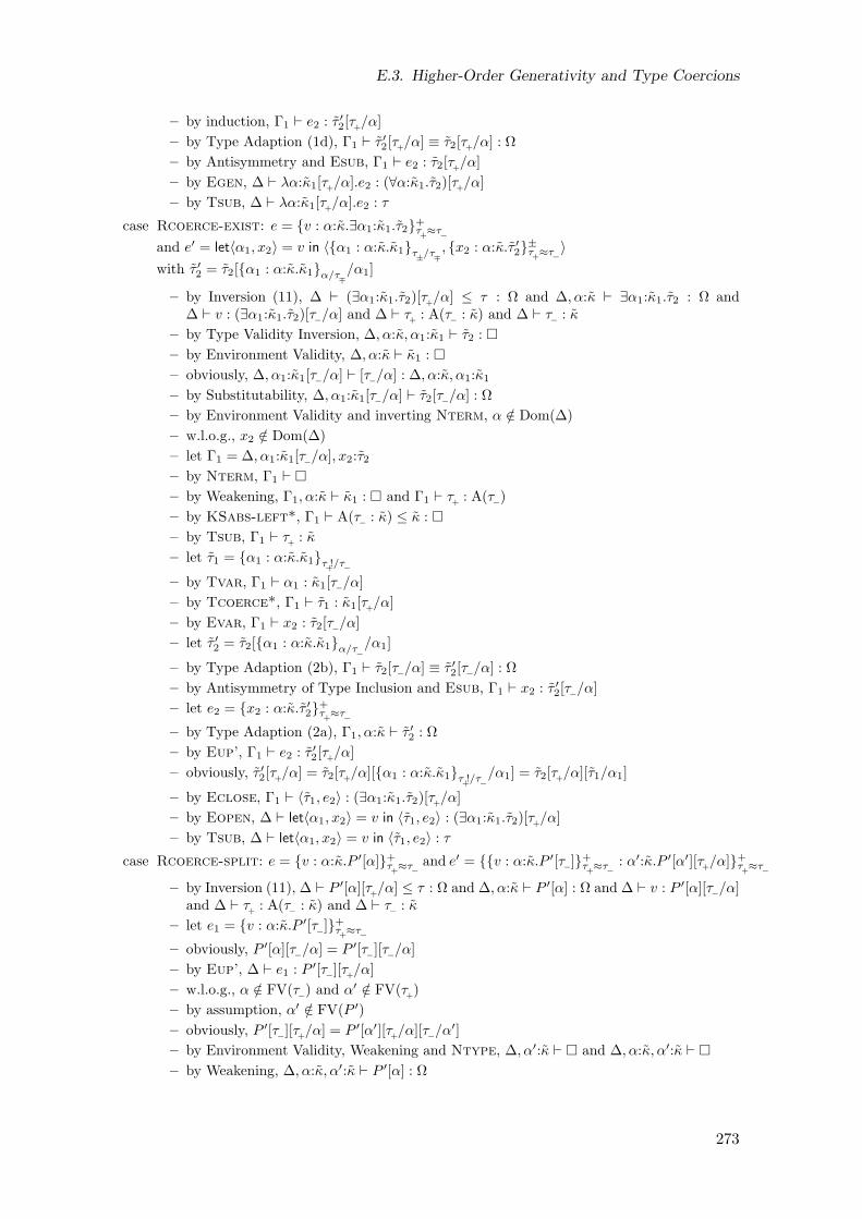
E.3. Higher-Order Generativity and Type Coercions
– by induction, Γ1 ⊢ e2 : τ ′2[τ+/α]
– by Type Adaption (1d), Γ1 ⊢ τ ′2[τ+/α] ≡ τ2[τ+/α] : Ω
– by Antisymmetry and Esub, Γ1 ⊢ e2 : τ2[τ+/α]
– by Egen, ∆ ⊢ λα:κ1[τ+/α].e2 : (∀α:κ1.τ2)[τ+/α]
– by Tsub, ∆ ⊢ λα:κ1[τ+/α].e2 : τ
case Rcoerce-exist: e = v : α:κ.∃α1:κ1.τ2+τ+≈τ
−
and e′ = let〈α1, x2〉 = v in 〈α1 : α:κ.κ1τ±
/τ∓, x2 : α:κ.τ ′2
±τ+≈τ−
〉
with τ ′2 = τ2[α1 : α:κ.κ1α/τ∓/α1]
– by Inversion (11), ∆ ⊢ (∃α1:κ1.τ2)[τ+/α] ≤ τ : Ω and ∆, α:κ ⊢ ∃α1:κ1.τ2 : Ω and∆ ⊢ v : (∃α1:κ1.τ2)[τ−/α] and ∆ ⊢ τ+ : A(τ− : κ) and ∆ ⊢ τ− : κ
– by Type Validity Inversion, ∆, α:κ, α1:κ1 ⊢ τ2 :
– by Environment Validity, ∆, α:κ ⊢ κ1 :
– obviously, ∆, α1:κ1[τ−/α] ⊢ [τ−/α] : ∆, α:κ, α1:κ1
– by Substitutability, ∆, α1:κ1[τ−/α] ⊢ τ2[τ−/α] : Ω
– by Environment Validity and inverting Nterm, α /∈ Dom(∆)
– w.l.o.g., x2 /∈ Dom(∆)
– let Γ1 = ∆, α1:κ1[τ−/α], x2:τ2
– by Nterm, Γ1 ⊢
– by Weakening, Γ1, α:κ ⊢ κ1 : and Γ1 ⊢ τ+
: A(τ−)
– by KSabs-left*, Γ1 ⊢ A(τ− : κ) ≤ κ :
– by Tsub, Γ1 ⊢ τ+
: κ
– let τ1 = α1 : α:κ.κ1τ+!/τ−
– by Tvar, Γ1 ⊢ α1 : κ1[τ−/α]
– by Tcoerce*, Γ1 ⊢ τ1 : κ1[τ+/α]
– by Evar, Γ1 ⊢ x2 : τ2[τ−/α]
– let τ ′2 = τ2[α1 : α:κ.κ1α/τ−/α1]
– by Type Adaption (2b), Γ1 ⊢ τ2[τ−/α] ≡ τ ′2[τ−/α] : Ω
– by Antisymmetry of Type Inclusion and Esub, Γ1 ⊢ x2 : τ ′2[τ−/α]
– let e2 = x2 : α:κ.τ ′2+τ+≈τ−
– by Type Adaption (2a), Γ1, α:κ ⊢ τ ′2 : Ω
– by Eup’, Γ1 ⊢ e2 : τ ′2[τ+/α]
– obviously, τ ′2[τ+/α] = τ2[τ+/α][α1 : α:κ.κ1τ+!/τ−
/α1] = τ2[τ+/α][τ1/α1]
– by Eclose, Γ1 ⊢ 〈τ1, e2〉 : (∃α1:κ1.τ2)[τ+/α]
– by Eopen, ∆ ⊢ let〈α1, x2〉 = v in 〈τ1, e2〉 : (∃α1:κ1.τ2)[τ+/α]
– by Tsub, ∆ ⊢ let〈α1, x2〉 = v in 〈τ1, e2〉 : τ
case Rcoerce-split: e = v : α:κ.P ′[α]+τ+≈τ
−and e′ = v : α:κ.P ′[τ−]+
τ+≈τ
−: α′:κ.P ′[α′][τ
+/α]+
τ+≈τ
−
– by Inversion (11), ∆ ⊢ P ′[α][τ+/α] ≤ τ : Ω and ∆, α:κ ⊢ P ′[α] : Ω and ∆ ⊢ v : P ′[α][τ−/α]
and ∆ ⊢ τ+ : A(τ− : κ) and ∆ ⊢ τ− : κ
– let e1 = v : α:κ.P ′[τ−]+τ+≈τ−
– obviously, P ′[α][τ−/α] = P ′[τ−][τ−/α]
– by Eup’, ∆ ⊢ e1 : P ′[τ−][τ+/α]
– w.l.o.g., α /∈ FV(τ−) and α′ /∈ FV(τ+)
– by assumption, α′ /∈ FV(P ′)
– obviously, P ′[τ−][τ+/α] = P ′[α′][τ
+/α][τ−/α
′]
– by Environment Validity, Weakening and Ntype, ∆, α′:κ ⊢ and ∆, α:κ, α′:κ ⊢
– by Weakening, ∆, α:κ, α′:κ ⊢ P ′[α] : Ω
273
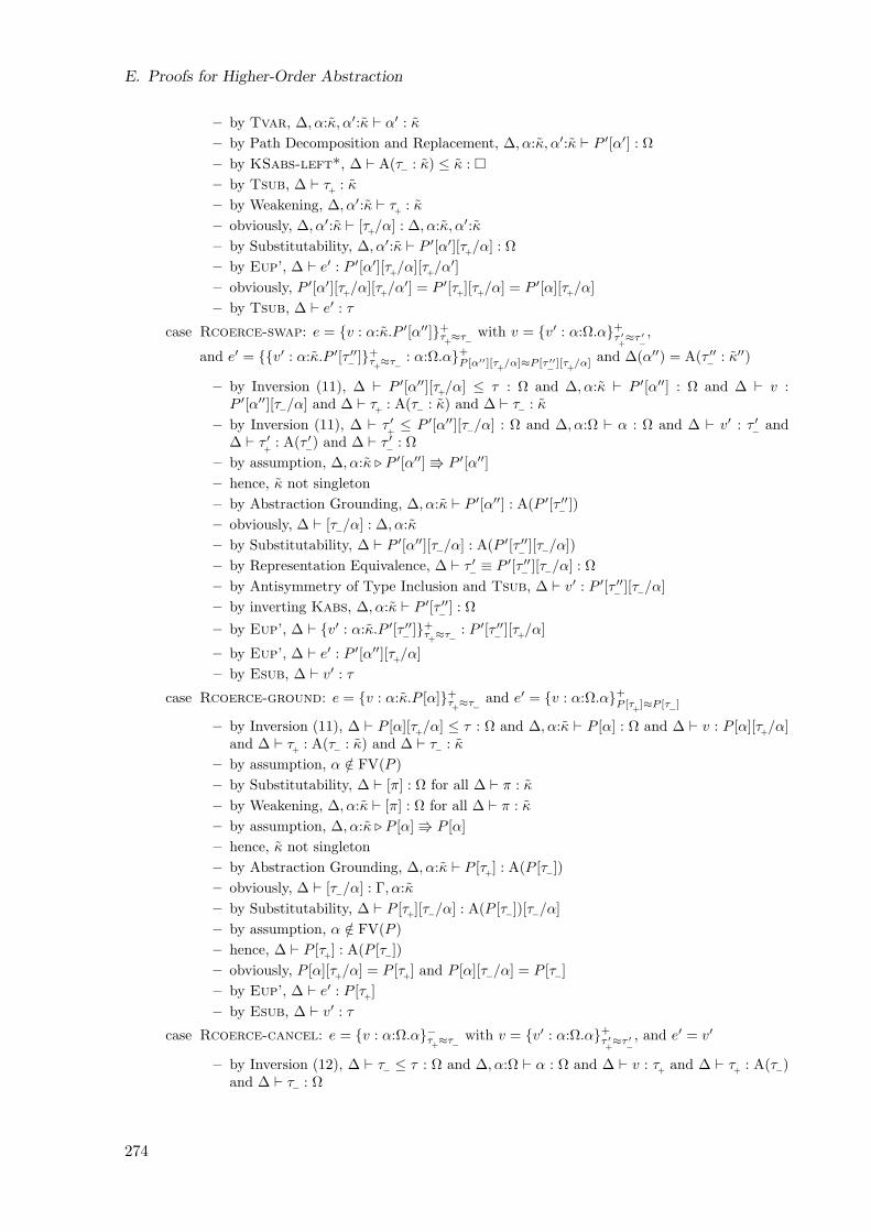
E. Proofs for Higher-Order Abstraction
– by Tvar, ∆, α:κ, α′:κ ⊢ α′ : κ
– by Path Decomposition and Replacement, ∆, α:κ, α′:κ ⊢ P ′[α′] : Ω
– by KSabs-left*, ∆ ⊢ A(τ− : κ) ≤ κ :
– by Tsub, ∆ ⊢ τ+ : κ
– by Weakening, ∆, α′:κ ⊢ τ+
: κ
– obviously, ∆, α′:κ ⊢ [τ+/α] : ∆, α:κ, α′:κ
– by Substitutability, ∆, α′:κ ⊢ P ′[α′][τ+/α] : Ω
– by Eup’, ∆ ⊢ e′ : P ′[α′][τ+/α][τ
+/α′]
– obviously, P ′[α′][τ+/α][τ+/α′] = P ′[τ+][τ+/α] = P ′[α][τ+/α]
– by Tsub, ∆ ⊢ e′ : τ
case Rcoerce-swap: e = v : α:κ.P ′[α′′]+τ+≈τ
−with v = v′ : α:Ω.α+
τ ′+≈τ ′
−,
and e′ = v′ : α:κ.P ′[τ ′′−
]+τ+≈τ
−: α:Ω.α+
P [α′′][τ+
/α]≈P [τ ′′−
][τ+
/α] and ∆(α′′) = A(τ ′′−
: κ′′)
– by Inversion (11), ∆ ⊢ P ′[α′′][τ+/α] ≤ τ : Ω and ∆, α:κ ⊢ P ′[α′′] : Ω and ∆ ⊢ v :P ′[α′′][τ−/α] and ∆ ⊢ τ
+: A(τ− : κ) and ∆ ⊢ τ− : κ
– by Inversion (11), ∆ ⊢ τ ′+≤ P ′[α′′][τ−/α] : Ω and ∆, α:Ω ⊢ α : Ω and ∆ ⊢ v′ : τ ′
−and
∆ ⊢ τ ′+
: A(τ ′−) and ∆ ⊢ τ ′
−: Ω
– by assumption, ∆, α:κ ⊲ P ′[α′′] P ′[α′′]
– hence, κ not singleton
– by Abstraction Grounding, ∆, α:κ ⊢ P ′[α′′] : A(P ′[τ ′′−
])
– obviously, ∆ ⊢ [τ−/α] : ∆, α:κ
– by Substitutability, ∆ ⊢ P ′[α′′][τ−/α] : A(P ′[τ ′′−
][τ−/α])
– by Representation Equivalence, ∆ ⊢ τ ′−≡ P ′[τ ′′
−][τ−/α] : Ω
– by Antisymmetry of Type Inclusion and Tsub, ∆ ⊢ v′ : P ′[τ ′′−
][τ−/α]
– by inverting Kabs, ∆, α:κ ⊢ P ′[τ ′′−
] : Ω
– by Eup’, ∆ ⊢ v′ : α:κ.P ′[τ ′′−
]+τ+≈τ
−: P ′[τ ′′
−][τ
+/α]
– by Eup’, ∆ ⊢ e′ : P ′[α′′][τ+/α]
– by Esub, ∆ ⊢ v′ : τ
case Rcoerce-ground: e = v : α:κ.P [α]+τ+≈τ
−and e′ = v : α:Ω.α+
P [τ+]≈P [τ
−]
– by Inversion (11), ∆ ⊢ P [α][τ+/α] ≤ τ : Ω and ∆, α:κ ⊢ P [α] : Ω and ∆ ⊢ v : P [α][τ
+/α]
and ∆ ⊢ τ+
: A(τ− : κ) and ∆ ⊢ τ− : κ
– by assumption, α /∈ FV(P )
– by Substitutability, ∆ ⊢ [π] : Ω for all ∆ ⊢ π : κ
– by Weakening, ∆, α:κ ⊢ [π] : Ω for all ∆ ⊢ π : κ
– by assumption, ∆, α:κ ⊲ P [α] P [α]
– hence, κ not singleton
– by Abstraction Grounding, ∆, α:κ ⊢ P [τ+] : A(P [τ−])
– obviously, ∆ ⊢ [τ−/α] : Γ, α:κ
– by Substitutability, ∆ ⊢ P [τ+][τ−/α] : A(P [τ−])[τ−/α]
– by assumption, α /∈ FV(P )
– hence, ∆ ⊢ P [τ+] : A(P [τ−])
– obviously, P [α][τ+/α] = P [τ
+] and P [α][τ−/α] = P [τ−]
– by Eup’, ∆ ⊢ e′ : P [τ+]
– by Esub, ∆ ⊢ v′ : τ
case Rcoerce-cancel: e = v : α:Ω.α−τ+≈τ
−with v = v′ : α:Ω.α+
τ ′+≈τ ′
−, and e′ = v′
– by Inversion (12), ∆ ⊢ τ− ≤ τ : Ω and ∆, α:Ω ⊢ α : Ω and ∆ ⊢ v : τ+
and ∆ ⊢ τ+
: A(τ−)and ∆ ⊢ τ− : Ω
274
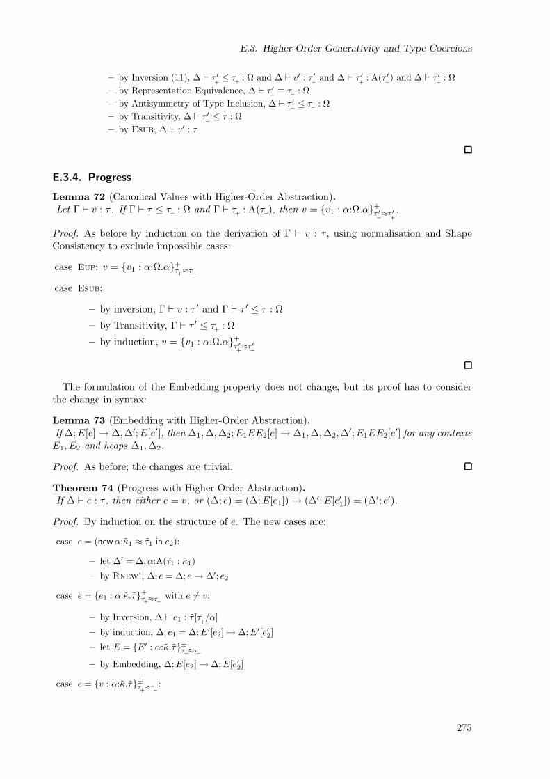
E.3. Higher-Order Generativity and Type Coercions
– by Inversion (11), ∆ ⊢ τ ′+≤ τ
+: Ω and ∆ ⊢ v′ : τ ′
−and ∆ ⊢ τ ′
+: A(τ ′
−) and ∆ ⊢ τ ′
−: Ω
– by Representation Equivalence, ∆ ⊢ τ ′−≡ τ− : Ω
– by Antisymmetry of Type Inclusion, ∆ ⊢ τ ′−≤ τ− : Ω
– by Transitivity, ∆ ⊢ τ ′−≤ τ : Ω
– by Esub, ∆ ⊢ v′ : τ
E.3.4. Progress
Lemma 72 (Canonical Values with Higher-Order Abstraction).Let Γ ⊢ v : τ . If Γ ⊢ τ ≤ τ
+: Ω and Γ ⊢ τ
+: A(τ−), then v = v1 : α:Ω.α+
τ ′−≈τ ′
+
.
Proof. As before by induction on the derivation of Γ ⊢ v : τ , using normalisation and ShapeConsistency to exclude impossible cases:
case Eup: v = v1 : α:Ω.α+τ+≈τ−
case Esub:
– by inversion, Γ ⊢ v : τ ′ and Γ ⊢ τ ′ ≤ τ : Ω
– by Transitivity, Γ ⊢ τ ′ ≤ τ+
: Ω
– by induction, v = v1 : α:Ω.α+τ ′+≈τ ′
−
The formulation of the Embedding property does not change, but its proof has to considerthe change in syntax:
Lemma 73 (Embedding with Higher-Order Abstraction).If ∆;E[e] → ∆,∆′;E[e′], then ∆1,∆,∆2;E1EE2[e] → ∆1,∆,∆2,∆
′;E1EE2[e′] for any contexts
E1, E2 and heaps ∆1,∆2.
Proof. As before; the changes are trivial.
Theorem 74 (Progress with Higher-Order Abstraction).If ∆ ⊢ e : τ , then either e = v, or (∆; e) = (∆;E[e1]) → (∆′;E[e′1]) = (∆′; e′).
Proof. By induction on the structure of e. The new cases are:
case e = (newα:κ1 ≈ τ1 in e2):
– let ∆′ = ∆, α:A(τ1 : κ1)
– by Rnew’, ∆; e = ∆; e→ ∆′; e2
case e = e1 : α:κ.τ±τ+≈τ−
with e 6= v:
– by Inversion, ∆ ⊢ e1 : τ [τ∓/α]
– by induction, ∆; e1 = ∆;E′[e2] → ∆;E′[e′2]
– let E = E′ : α:κ.τ±τ+≈τ−
– by Embedding, ∆;E[e2] → ∆;E[e′2]
case e = v : α:κ.τ±τ+≈τ
−:
275
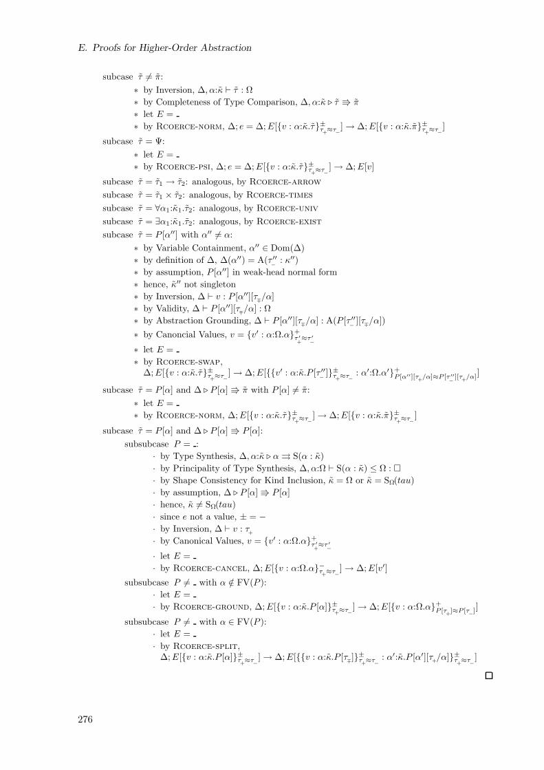
E. Proofs for Higher-Order Abstraction
subcase τ 6= π:
∗ by Inversion, ∆, α:κ ⊢ τ : Ω
∗ by Completeness of Type Comparison, ∆, α:κ ⊲ τ π
∗ let E =
∗ by Rcoerce-norm, ∆; e = ∆;E[v : α:κ.τ±τ+≈τ
−] → ∆;E[v : α:κ.π±τ
+≈τ
−]
subcase τ = Ψ:
∗ let E =
∗ by Rcoerce-psi, ∆; e = ∆;E[v : α:κ.τ±τ+≈τ−
] → ∆;E[v]
subcase τ = τ1 → τ2: analogous, by Rcoerce-arrow
subcase τ = τ1 × τ2: analogous, by Rcoerce-times
subcase τ = ∀α1:κ1.τ2: analogous, by Rcoerce-univ
subcase τ = ∃α1:κ1.τ2: analogous, by Rcoerce-exist
subcase τ = P [α′′] with α′′ 6= α:
∗ by Variable Containment, α′′ ∈ Dom(∆)
∗ by definition of ∆, ∆(α′′) = A(τ ′′−
: κ′′)
∗ by assumption, P [α′′] in weak-head normal form
∗ hence, κ′′ not singleton
∗ by Inversion, ∆ ⊢ v : P [α′′][τ∓/α]
∗ by Validity, ∆ ⊢ P [α′′][τ∓/α] : Ω
∗ by Abstraction Grounding, ∆ ⊢ P [α′′][τ∓/α] : A(P [τ ′′−
][τ∓/α])
∗ by Canoncial Values, v = v′ : α:Ω.α+τ ′+≈τ ′
−
∗ let E =
∗ by Rcoerce-swap,∆;E[v : α:κ.τ±τ
+≈τ−
] → ∆;E[v′ : α:κ.P [τ ′′−
]±τ+≈τ−
: α′:Ω.α′+P [α′′][τ
+/α]≈P [τ ′′
−][τ
+/α]]
subcase τ = P [α] and ∆ ⊲ P [α] π with P [α] 6= π:
∗ let E =
∗ by Rcoerce-norm, ∆;E[v : α:κ.τ±τ+≈τ
−] → ∆;E[v : α:κ.π±τ
+≈τ
−]
subcase τ = P [α] and ∆ ⊲ P [α] P [α]:
subsubcase P = :
· by Type Synthesis, ∆, α:κ ⊲ α S(α : κ)
· by Principality of Type Synthesis, ∆, α:Ω ⊢ S(α : κ) ≤ Ω :
· by Shape Consistency for Kind Inclusion, κ = Ω or κ = SΩ(tau)
· by assumption, ∆ ⊲ P [α] P [α]
· hence, κ 6= SΩ(tau)
· since e not a value, ± = −
· by Inversion, ∆ ⊢ v : τ+
· by Canonical Values, v = v′ : α:Ω.α+τ ′+≈τ ′
−
· let E =
· by Rcoerce-cancel, ∆;E[v : α:Ω.α−τ+≈τ
−] → ∆;E[v′]
subsubcase P 6= with α /∈ FV(P ):
· let E =
· by Rcoerce-ground, ∆;E[v : α:κ.P [α]±τ+≈τ−
] → ∆;E[v : α:Ω.α+P [τ
+]≈P [τ
−]]
subsubcase P 6= with α ∈ FV(P ):
· let E =
· by Rcoerce-split,∆;E[v : α:κ.P [α]±τ
+≈τ
−] → ∆;E[v : α:κ.P [τ∓]±τ
+≈τ
−: α′:κ.P [α′][τ
+/α]±τ
+≈τ
−]
276
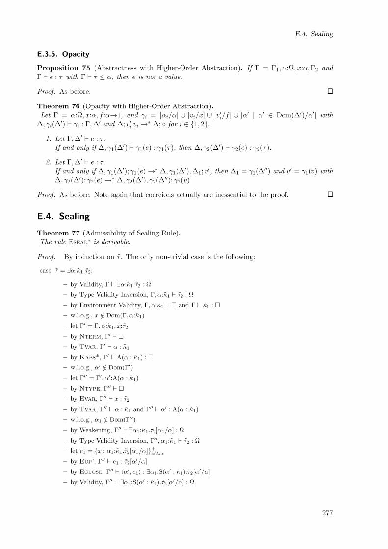
E.4. Sealing
E.3.5. Opacity
Proposition 75 (Abstractness with Higher-Order Abstraction). If Γ = Γ1, α:Ω, x:α,Γ2 andΓ ⊢ e : τ with Γ ⊢ τ ≤ α, then e is not a value.
Proof. As before.
Theorem 76 (Opacity with Higher-Order Abstraction).Let Γ = α:Ω, x:α, f :α→1, and γi = [αi/α] ∪ [vi/x] ∪ [v′i/f ] ∪ [α′ | α′ ∈ Dom(∆′)/α′] with
∆, γi(∆′) ⊢ γi : Γ,∆′ and ∆; v′i vi →
∗ ∆; ⋄ for i ∈ 1, 2.
1. Let Γ,∆′ ⊢ e : τ .If and only if ∆, γ1(∆
′) ⊢ γ1(e) : γ1(τ), then ∆, γ2(∆′) ⊢ γ2(e) : γ2(τ).
2. Let Γ,∆′ ⊢ e : τ .If and only if ∆, γ1(∆
′); γ1(e) →∗ ∆, γ1(∆
′),∆1; v′, then ∆1 = γ1(∆
′′) and v′ = γ1(v) with∆, γ2(∆
′); γ2(e) →∗ ∆, γ2(∆
′), γ2(∆′′); γ2(v).
Proof. As before. Note again that coercions actually are inessential to the proof.
E.4. Sealing
Theorem 77 (Admissibility of Sealing Rule).The rule Eseal* is derivable.
Proof. By induction on τ . The only non-trivial case is the following:
case τ = ∃α:κ1.τ2:
– by Validity, Γ ⊢ ∃α:κ1.τ2 : Ω
– by Type Validity Inversion, Γ, α:κ1 ⊢ τ2 : Ω
– by Environment Validity, Γ, α:κ1 ⊢ and Γ ⊢ κ1 :
– w.l.o.g., x /∈ Dom(Γ, α:κ1)
– let Γ′ = Γ, α:κ1, x:τ2
– by Nterm, Γ′ ⊢
– by Tvar, Γ′ ⊢ α : κ1
– by Kabs*, Γ′ ⊢ A(α : κ1) :
– w.l.o.g., α′ /∈ Dom(Γ′)
– let Γ′′ = Γ′, α′:A(α : κ1)
– by Ntype, Γ′′ ⊢
– by Evar, Γ′′ ⊢ x : τ2
– by Tvar, Γ′′ ⊢ α : κ1 and Γ′′ ⊢ α′ : A(α : κ1)
– w.l.o.g., α1 /∈ Dom(Γ′′)
– by Weakening, Γ′′ ⊢ ∃α1:κ1.τ2[α1/α] : Ω
– by Type Validity Inversion, Γ′′, α1:κ1 ⊢ τ2 : Ω
– let e1 = x : α1:κ1.τ2[α1/α]+α′≈α
– by Eup’, Γ′′ ⊢ e1 : τ2[α′/α]
– by Eclose, Γ′′ ⊢ 〈α′, e1〉 : ∃α1:S(α′ : κ1).τ2[α′/α]
– by Validity, Γ′′ ⊢ ∃α1:S(α′ : κ1).τ2[α′/α] : Ω
277
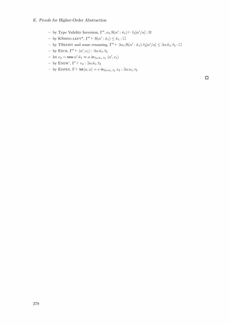
E. Proofs for Higher-Order Abstraction
– by Type Validity Inversion, Γ′′, α1:S(α′ : κ1) ⊢ τ2[α′/α] : Ω
– by KSsing-left*, Γ′′ ⊢ S(α′ : κ1) ≤ κ1 :
– by TSexist and some renaming, Γ′′ ⊢ ∃α1:S(α′ : κ1).τ2[α′/α] ≤ ∃α:κ1.τ2 :
– by Esub, Γ′′ ⊢ 〈α′, e1〉 : ∃α:κ1.τ2
– let e2 = newα′:κ1 ≈ α in∃α:κ1.τ2 〈α′, e1〉
– by Enew’, Γ′ ⊢ e2 : ∃α:κ1.τ2
– by Eopen, Γ ⊢ let〈α, x〉 = e in∃α:κ1.τ2 e2 : ∃α:κ1.τ2
278
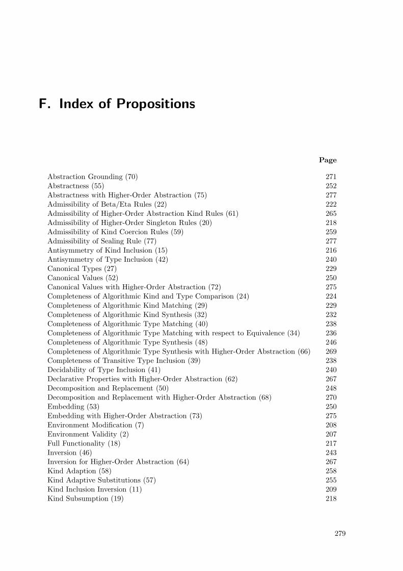
F. Index of Propositions
Page
Abstraction Grounding (70) 271Abstractness (55) 252Abstractness with Higher-Order Abstraction (75) 277Admissibility of Beta/Eta Rules (22) 222Admissibility of Higher-Order Abstraction Kind Rules (61) 265Admissibility of Higher-Order Singleton Rules (20) 218Admissibility of Kind Coercion Rules (59) 259Admissibility of Sealing Rule (77) 277Antisymmetry of Kind Inclusion (15) 216Antisymmetry of Type Inclusion (42) 240Canonical Types (27) 229Canonical Values (52) 250Canonical Values with Higher-Order Abstraction (72) 275Completeness of Algorithmic Kind and Type Comparison (24) 224Completeness of Algorithmic Kind Matching (29) 229Completeness of Algorithmic Kind Synthesis (32) 232Completeness of Algorithmic Type Matching (40) 238Completeness of Algorithmic Type Matching with respect to Equivalence (34) 236Completeness of Algorithmic Type Synthesis (48) 246Completeness of Algorithmic Type Synthesis with Higher-Order Abstraction (66) 269Completeness of Transitive Type Inclusion (39) 238Decidability of Type Inclusion (41) 240Declarative Properties with Higher-Order Abstraction (62) 267Decomposition and Replacement (50) 248Decomposition and Replacement with Higher-Order Abstraction (68) 270Embedding (53) 250Embedding with Higher-Order Abstraction (73) 275Environment Modification (7) 208Environment Validity (2) 207Full Functionality (18) 217Inversion (46) 243Inversion for Higher-Order Abstraction (64) 267Kind Adaption (58) 258Kind Adaptive Substitutions (57) 255Kind Inclusion Inversion (11) 209Kind Subsumption (19) 218
279
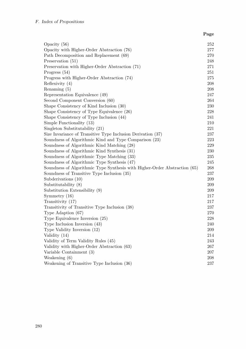
F. Index of Propositions
Page
Opacity (56) 252Opacity with Higher-Order Abstraction (76) 277Path Decomposition and Replacement (69) 270Preservation (51) 248Preservation with Higher-Order Abstraction (71) 271Progress (54) 251Progress with Higher-Order Abstraction (74) 275Reflexivity (4) 208Renaming (5) 208Representation Equivalence (49) 247Second Component Conversion (60) 264Shape Consistency of Kind Inclusion (30) 230Shape Consistency of Type Equivalence (26) 228Shape Consistency of Type Inclusion (44) 241Simple Functionality (13) 210Singleton Substitutability (21) 221Size Invariance of Transitive Type Inclusion Derivation (37) 237Soundness of Algorithmic Kind and Type Comparison (23) 223Soundness of Algorithmic Kind Matching (28) 229Soundness of Algorithmic Kind Synthesis (31) 230Soundness of Algorithmic Type Matching (33) 235Soundness of Algorithmic Type Synthesis (47) 245Soundness of Algorithmic Type Synthesis with Higher-Order Abstraction (65) 268Soundness of Transitive Type Inclusion (35) 237Subderivations (10) 209Substitutability (8) 209Substitution Extensibility (9) 209Symmetry (16) 217Transitivity (17) 217Transitivity of Transitive Type Inclusion (38) 237Type Adaption (67) 270Type Equivalence Inversion (25) 228Type Inclusion Inversion (43) 240Type Validity Inversion (12) 209Validity (14) 214Validity of Term Validity Rules (45) 243Validity with Higher-Order Abstraction (63) 267Variable Containment (3) 207Weakening (6) 208Weakening of Transitive Type Inclusion (36) 237
280
Bibliography
[ACC93] Martın Abadi, Luca Cardelli, and Pierre-Louis Curien. Formal parametric poly-morphism. Theoretical Computer Science, 121:9–58, 1993.
[ACG86] Sudhir Ahuja, Nicholas Carriero, and David Gelernter. Linda and friends. IEEEComputer, 19(8):26–34, August 1986.
[ACPP89] Martın Abadi, Luca Cardelli, Benjamin Pierce, and Gordon Plotkin. Dynamic typ-ing in a statically-typed language. In 16th Symposium on Principles of ProgrammingLanguages, pages 213–227, Austin, USA, January 1989.
[ACPP91] Martın Abadi, Luca Cardelli, Benjamin Pierce, and Gordon Plotkin. Dynamictyping in a statically-typed language. Transactions on Programming Languagesand Systems, 13(2):237–268, April 1991.
[ACPR95] Martın Abadi, Luca Cardelli, Benjamin Pierce, and Didier Remy. Dynamic typing inpolymorphic languages. Journal of Functional Programming, 5(1):111–130, January1995.
[AFZ04] Davide Ancona, Sonia Fagorzi, and Elena Zucca. A calculus with lazy moduleoperators. In Jean-Jacques Levy, Ernst Mayr, and John Mitchell, editors, 3rdInternational Conference on Theoretical Computer Science, pages 423–436. KluwerAcademic Publishers, 2004.
[Ala04] Lauri Alanko. Types and reflection. Master’s thesis, Helsingin Yliopisto, Helsinki,Finland, November 2004.
[Ali03] Alice Team. The Alice System. Programming Systems Lab, Universitat des Saar-landes, http://www.ps.un-sb.de/alice/, 2003.
[ANP89] Arvind, Rishiyur Nikhil, and Keshav Pingali. I-structures: data structures for par-allel computing. Transactions on Programming Languages and Systems, 11(4):598–632, 1989.
[Apt03] Krysztof Apt. Principles of Constraint Programming. Cambridge University Press,2003.
[Arm03] Joe Armstrong. Making Reliable Distributed Systems in the Presence of SoftwareErrors. Doctoral dissertation, Royal Institute of Technology, Stockholm, Sweden,December 2003.
[Asp95] David Aspinall. Subtyping with singleton types. In Computer Science Logic, volume933 of Lecture Notes in Computer Science. Springer-Verlag, 1995.
[Asp97] David Aspinall. Type Systems for Modular Programs and Specifications. PhD thesis,Edinburgh University, Edinburgh, UK, December 1997.
281
Bibliography
[AZ02] Davide Ancona and Elena Zucca. A calculus of module systems. Journal of Func-tional Programming, 12(2), 2002.
[BA99] Matthias Blume and Andrew Appel. Hierarchical modularity. Transactions onProgramming Languages and Systems, 21(4):813–847, July 1999.
[Bar92] Henk Barendregt. Lambda calculi with types. In Samson Abramsky, Dov Gabbay,and T.S.E. Maibaum, editors, Handbook of Logic in Computer Science, volume 2,chapter 2, pages 117–309. Oxford University Press, 1992.
[Ber04] Matthias Berg. Polymorphic lambda calculus with dynamic types. Fopra thesis,Universitat des Saarlandes, Saarbrucken, Germany, October 2004.
[BFSS89] E.S. Bainbridge, Peter Freyd, Andre Scedrov, and Philip Scott. Functorial polymor-phism. Theoretical Computer Science, 70(1):35–64, 1989. Corrigendum in 71(3):431,1990.
[BHS+03] Gavin Bierman, Michael Hicks, Peter Sewell, Gareth Stoyle, and Keith Wansbrough.Dynamic rebinding for marshalling and update, with destruct-time lambda. In 8thInternational Conference on Functional Programming, Uppsala, Sweden, September2003.
[BJW87] Andrew Birrell, Michael Jones, and Edwar Wobber. A simple and efficient im-plementation for small databases. In 11th ACM Symposium on Operating SystemPrinciples, volume 21(5) of Operating Systems Review, pages 149–154. ACM Press,November 1987.
[BK02] Thorsten Brunklaus and Leif Kornstaedt. A virtual machine for multi-languageexecution. Technical report, Programming Systems Lab, Universitat des Saarlandes,Saarbrucken, Germany, November 2002.
[BK03] Thorsten Brunklaus and Leif Kornstaedt. Open programming services for virtualmachines: The design of Mozart and SEAM. Technical report, Programming Sys-tems Lab, Universitat des Saarlandes, Saarbrucken, Germany, March 2003.
[BN84] Andrew Birrell and Bruce Nelson. Implementing remote procedure calls. Transac-tions on Computer Systems, 2(1):39–59, 1984.
[BNOW95] Andrew Birrell, Greg Nelson, Susan Owicki, and Edward Wobbler. Network objects.Software – Practice and Experience, 25(S4), December 1995.
[BNSS94] Peter Bailey, Malcolm Newey, David Sitsky, and Robin Stanton. Supporting coarseand fine grain parallelism in an extension of ML. In Conference on Algorithmsand Hardware for Parallel Processing, volume 854 of Lecture Notes in ComputerScience, pages 693–704. Springer-Verlag, 1994.
[Bur84] Rod Burstall. Programming with modules as typed functional programming. InInternational Conference on 5th Generation Computing Systems, Tokyo, Japan,1984.
[Car91] Luca Cardelli. Typeful programming. In E. J. Neuhold and M. Paul, editors, For-mal Description of Programming Concepts, pages 431–507. Springer-Verlag, Berlin,Germany, 1991.
282
Bibliography
[Car95] Luca Cardelli. A language with distributed scope. Computing Systems, 8(1):27–59,January 1995.
[Car97a] Luca Cardelli. Program fragments, linking, and modularization. In 24th Symposiumon Principles of Programming Languages, pages 266–277, Paris, France, January1997.
[Car97b] Luca Cardelli. Type systems. In Allen Tucker, editor, The Computer Science andEngineering Handbook, chapter 103, pages 2208–2236. CRC Press, 1997.
[CDG+91] Luca Cardelli, James Donahue, Lucille Glassman, Mick Jordan, Bill Kalsow, andGreg Nelson. Modula-3 language definition. In Greg Nelson, editor, System Pro-gramming with Modula-3, chapter 2, pages 11–66. Prentice Hall, 1991.
[CK92] Robert Cooper and Clifford Krumvieda. Distributed programming with asyn-chronous ordered channels in distributed ML. In Peter Lee, editor, Workshop onML and its Applications, pages 134–148, June 1992.
[CL90] Luca Cardelli and Xavier Leroy. Abstract types and the dot notation. In IFIPTC2 working conference on programming concepts and methods, pages 479–504.North-Holland, March 1990.
[CL99] Sylvain Conchon and Fabrice Le Fessant. Jocaml: mobile agents for objective-caml. In First International Symposium on Agent Systems and Applications andThird International Symposium on Mobile Agents, pages 22–29, Palm Springs, USA,October 1999.
[Cra00] Karl Crary. Typed compilation of inclusive subtyping. In 5th International Con-ference on Functional Programming, Montreal, Canada, September 2000.
[CW99] Karl Crary and Stephanie Weirich. Flexible type analysis. In 5th InternationalConference on Functional Programming, pages 233–248, Paris, France, October1999.
[CWM98] Karl Crary, Stephanie Weirich, and Greg Morisett. Intensional polymorphism intype-erasure semantics. In 3rd International Conference on Functional Program-ming, Baltimore, USA, September 1998.
[CWM02] Karl Crary, Stephanie Weirich, and Greg Morrisett. Intensional polymorphism intype erasure semantics. Journal of Functional Programming, 12(6):567–600, Novem-ber 2002.
[DCH03] Derek Dreyer, Karl Crary, and Robert Harper. A type system for higher-order mod-ules. In 30th Symposium on Principles of Programming Languages, New Orleans,USA, January 2003.
[Dea97] Drew Dean. The security of static typing with dynamic linking. In 4th Conferenceon Computer and Communications Security, pages 18–27, 1997.
[Den85] Peter Denning, editor. Special Issue on Prolog, volume 28(12) of Communicationsof the ACM. ACM Press, December 1985.
[DFW96] Drew Dean, Edward Felten, and Dan Wallach. Java security: from HotJava toNetscape and beyond. In Symposium on Security and Privacy, pages 190–200,Oakland, USA, May 1996. IEEE Computer Society Press.
283
Bibliography
[DG04] Jeffrey Dean and Sanjay Ghemawat. Mapreduce: Simplified data processing onlarge clusters. In Operating Systems Design and Implementation, San Francisco,USA, 2004.
[DHC01] Derek Dreyer, Robert Harper, and Karl Crary. Toward a practical type theory forrecursive modules. Technical Report CMU-CS-01-112, School of Computer Science,Carnegie Mellon University, Pittsburgh, USA, March 2001.
[DKSS98] Denys Duchier, Leif Kornstaedt, Christian Schulte, and Gert Smolka. A higher-order module discipline with separate compilation, dynamic linking, and pick-ling. Technical report, Programming Systems Lab, Universitat des Saarlandes,Saarbrucken, Germany, 1998. Draft, http://www.ps.uni-sb.de/papers.
[DM82] Luis Damas and Robin Milner. Principal type-schemes for functional programs. InRichard DeMillo, editor, 7th Symposium on Principles of Programming Languages,pages 207–212, Albuquerque, USA, January 1982. ACM Press.
[Dre04] Derek Dreyer. A type system for well-founded recursion. In 31st Symposium onPrinciples of Programming Languages, Venice, Italy, January 2004.
[Dre05] Derek Dreyer. Understanding and Evolving the ML Module System. Phd thesis,Carnegie Mellon University, 2005.
[Dre07] Derek Dreyer. Recursive type generativity. Journal of Functional Programming,Forthcoming 2007.
[DRW95] Catherine Dubois, Francois Rouaix, and Pierre Weis. Extensional polymorphism.In 22nd Symposium on Principles of Programming Languages, San Francisco, USA,January 1995.
[Dug99] Dominic Duggan. Dynamic typing for distributed programming in polymorphiclanguages. Transactions on Programming Languages and Systems, 21(1):11–45,1999.
[Dug02] Dominic Duggan. Type-safe linking with recursive DLLs and shared libraries. Trans-action on Programming Languages and Systems, 24(6):711–804, November 2002.
[Els99] Martin Elsman. Static interpretation of modules. In Fourth International Confer-ence on Functional Programming, pages 208–219, Paris, France, September 1999.ACM Press.
[FF95] Cormac Flanagan and Matthias Felleisen. The semantics of future and its use in pro-gram optimizations. In 22nd Symposium on Principles of Programming Languages,pages 209–220, San Francisco, USA, January 1995.
[FF98] Matthew Flatt and Matthias Felleisen. Units: Cool modules for HOT languages.In Programming Language Design and Implementation, pages 236–248, Montreal,Canada, June 1998.
[FGL+96] Cedric Fournet, Georges Gonthier, Jean-Jacques Levy, Luc Maranget, and DidierRemy. On distributed programming: A calculus of mobile agents. In 7th Interna-tional Conference on Concurrency Theory, volume 1119 of Lecture Notes in Com-puter Science, pages 278–298. Springer-Verlag, 1996.
284
Bibliography
[FMS01] Cedric Fournet, Luc Maranget, and Alan Schmitt. The JoCaml Language betarelease. INRIA, http://pauillac.inria.fr/jocaml/htmlman/, January 2001.
[FW76] Daniel Friedman and David Wise. CONS should not evaluate its arguments. InS. Michaelson and Robin Milner, editors, Third International Colloquium on Au-tomata, Languages, and Programming, pages 257–284. Edinburgh University Press,July 1976.
[Gec05] Gecode Team. Generic constraint development environment, 2005. http://www.
gecode.org/.
[Gir71] Jean-Yves Girard. Une extension de l’interpretation de Godel a l’analysis, et son ap-plication a l’elimination des coupures dans l’analysis et la theorie des types. In J. E.Fenstad, editor, Proceedings 2nd Scandinavian Logic Symposium. North-Holland,1971.
[GJS96] James Gosling, Bill Joy, and Guy Steele. The Java Programming Language Speci-fication. Addison–Wesley, 1996.
[Gle99] Neal Glew. Type dispatch for named hierarchical types. In 5th International Con-ference on Functional Programming, Paris, France, October 1999.
[GM99] Neal Glew and Greg Morrisett. Type-safe linking and modular assembly language.In 26th Symposium on Principles of Programming Languages, pages 250–261, Jan-uary 1999.
[GMW79] Michael Gordon, Robin Milner, and Christopher Wadsworth. Edinburgh LCF: AMechanized Logic of Computation, volume 78 of Lecture Notes in Computer Science.Springer-Verlag, 1979.
[GMZ00] Dan Grossman, Greg Morrisett, and Steve Zdancewic. Syntactic type abstraction.Transactions on Programming Languages and Systems, 22(6):1037–1080, November2000.
[GP98] Giorgio Ghelli and Benjamin Pierce. Bounded existentials and minimal typing.Theoretical Computer Science, 193(1–2):75–96, February 1998.
[GR04] Emden Gansner and John Reppy. The Standard ML Basis Library. CambridgeUniversity Press, 2004.
[Hal85] Robert Halstead. Multilisp: A language for concurrent symbolic computation.Transactions on Programming Languages and Systems, 7(4):501–538, October 1985.
[Har06] Robert Harper. Programming in Standard ML. Draft, 2006.
[HBS73] Carl Hewitt, Peter Bishop, and Richard Steiger. A universal, modular actor for-malism for artificial intelligence. In 3rd International Joint Conference on ArtificialIntelligence, pages 235–245, 1973.
[HCS+01] Fergus Henderson, Thomas Conway, Zoltan Somogyi, David Jefferey, PeterSchachte, Simon Taylor, and Chris Speirs. The Mercury Language Ref-erence Manual. http://www.cs.mu.oz.au/research/mercury/information/
documentation.html, 2001.
285
Bibliography
[Hin69] J.R. Hindley. The principal type-scheme of an object in combinatory logic. InTransactions of AMS, pages 146:29–60, 1969.
[HL82] Maurice Herlihy and Barbara Liskov. A value transmission method for abstractdata types. Transactions on Programming Languages and Systems, 4(4):527–551,October 1982.
[HL94] Robert Harper and Mark Lillibridge. A type-theoretic approach to higher-ordermodules with sharing. In 21st Symposium on Principles of Programming Languages,pages 123–137, Portland, USA, January 1994.
[HM93] Robert Harper and John Mitchell. On the type structure of Standard ML. Theoryof Programming Languages and Systems, 15(2):211–252, April 1993.
[HM95] Robert Harper and Greg Morrisett. Compiling polymorphism using intensionaltype analysis. In 22nd Symposium on Principles of Programming Languages, pages130–141, San Francisco, USA, January 1995.
[HM99] Robert Harper and John Mitchell. Parametricity and variants of Girard’s J operator.Information Processing Letters, 70(1):1–5, 1999.
[HMM90] Robert Harper, John Mitchell, and Eugenio Moggi. Higher-order modules and thephase distinction. In 17th Symposium on Principles of Programming Languages,pages 341–354, San Francisco, USA, January 1990.
[HMPH05] Tim Harris, Simon Marlow, Simon Peyton Jones, and Maurice Herlihy. Composablememory transactions. In Tenth ACM SIGPLAN Symposium on Principles andPractice of Parallel Programming, pages 48–60. ACM Press, 2005.
[HP05] Robert Harper and Benjamin Pierce. Design Considerations for ML-Style ModuleSystems, chapter 8, pages 293–345. The MIT Press, 2005.
[HR99] Michael Hansen and Hans Rischel. Introduction to Programming using SML.Addison-Wesley, 1999.
[HRB+99] Seif Haridi, Peter Van Roy, Per Brand, Michael Mehl, Ralf Scheidhauer, and GertSmolka. Efficient logic variables for distributed computing. Transactions on Pro-gramming Languages and Systems, 21(3):569–626, May 1999.
[HRBS98] Seif Haridi, Peter Van Roy, Per Brand, and Christian Schulte. Programming lan-guages for distributed applications. New Generation Computing, 16(3):223–261,1998.
[HS00] Robert Harper and Christopher Stone. A type-theoretic interpretation of StandardML. In Gordon Plotkin, Colin Stirling, and Mads Tofte, editors, Proof, Language,and Interaction: Essays in Honor of Robin Milner. MIT Press, 2000.
[Ken04] Andrew Kennedy. Pickler combinators. Journal of Functional Programming,14(6):727–739, November 2004.
[Kor06] Leif Kornstaedt. Design and Implementation of a Programmable Middleware. Doc-toral dissertation, Universitat des Saarlandes, Saarbrucken, Germany, December2006.
286
Bibliography
[LAB+79] Barbara Liskov, Russell Atkinson, Toby Bloom, Eliot Moss, Craig Schaffert,Robert Scheifler, and Alan Snyder. CLU reference manual. Technical ReportMIT/LCS/TR-225, Massachusetts Institute of Technology, 1979.
[LB98] Sheng Liang and Gilad Bracha. Dynamic class loading in the Java Virtual Machine.In Object-Oriented Programming, Systems, Languages and Applications, October1998.
[Ler92] Xavier Leroy. Unboxed objects and polymorphic typing. In 19th Symposium onPrinciples of Programming Languages, pages 177–188, New York, USA, January1992. ACM Press.
[Ler94] Xavier Leroy. Manifest types, modules, and separate compilation. In 21st Sym-posium on Principles of Programming Languages, pages 109–122, Portland, USA,January 1994. ACM.
[Ler95] Xavier Leroy. Applicative functors and fully transparent higher-order modules. In22nd Symposium on Principles of Programming Languages, pages 142–153, SanFrancisco, USA, January 1995. ACM.
[Ler03] Xavier Leroy. The Objective Caml System. INRIA, 2003. http://pauillac.inria.fr/ocaml/htmlman/.
[Lil97] Mark Lillibridge. Translucent Sums: A Foundation for Higher-Order Module Sys-tems. PhD thesis, School of Computer Science, Carnegie Mellon University, Pitts-burgh, USA, May 1997.
[LM93] Xavier Leroy and Michel Mauny. Dynamics in ML. Journal of Functional Program-ming, 3(4):431–463, 1993.
[LPSW03] James Leifer, Gilles Peskine, Peter Sewell, and Keith Wansbrough. Globalabstraction-safe marshalling with hash types. In 8th International Conference onFunctional Programming, Uppsala, Sweden, September 2003.
[LS88] Barbara Liskov and Liuba Shrira. Promises: linguistic support for efficient asyn-chronous procedure calls in distributed systems. In Programming Language Designand Implementation, pages 260–267. ACM Press, 1988.
[Luc00] Lucent Technologies. Standard ML of New Jersey User’s Guide. http://cm.
bell-labs.com/cm/cs/what/smlnj/doc/, 2000.
[LY96] Tim Lindholm and Frank Yellin. The Java Virtual Machine Specification. Addison–Wesley, 1996.
[Mac84] David MacQueen. Modules for Standard ML. In Symposium on LISP and Func-tional Programming, pages 198–207, Austin, USA, 1984.
[Mac86] David MacQueen. Using dependent types to express modular structure. In 13thSymposium on Principles of Programming Languages, pages 277–286, St. Peters-burg, USA, January 1986.
[Mac93] David MacQueen. Reflections on standard ML. In Functional Programming, Con-currency, Simulation and Automated Reasoning, pages 32–46, 1993.
287
Bibliography
[MG98] Yasuhiko Minamide and Jacque Garrigue. On the runtime complexity of type-directed unboxing. In 3rd International Conference on Functional Programming,Baltimore, USA, September 1998.
[Mic03] Microsoft Corporation. Microsoft .NET. http://www.microsoft.com/net/, 2003.
[Mil78] Robin Milner. A theory of type polymorphism. Journal of Computer and SystemsSciences, 17:348–375, 1978.
[Mil89] Robin Milner. Communication and Concurrency. Prentice-Hall, 1989.
[Mil99] Robin Milner. Communicating and Mobile Systems: the Pi-Calculus. CambridgeUniversity Press, 1999.
[Mil06] Mark Miller. Robust Composition: Towards a Unified Approach to Access Con-trol and Concurrency Control. Doctoral dissertation, Johns Hopkins University,Baltimore, USA, May 2006.
[Mit91] John Mitchell. On the equivalence of data representations. In Vladimir Lifschitz,editor, Artificial Intelligence and Mathematical Theory of Computation: Papers inHonor of John McCarthy, pages 305–330. Academic Press, 1991.
[ML71] Per Martin-Lof. A theory of types, 1971. Unpublished manuscript.
[MM91] John Mitchell and Eugenion Moggi. Kripke-style models for typed lambda calculus.Annals of Pure and Applied Logic, 51:99–124, 1991.
[Mor73a] James Morris. Protection in programming language. Communications of the ACM,16(1), January 1973.
[Mor73b] James Morris. Types are not sets. In 1st Symposium on Principles of ProgrammingLanguages, pages 120–124, Boston, USA, October 1973.
[Moz04] Mozart Consortium. The Mozart programming system, 2004. http://www.
mozart-oz.org.
[MP88] John Mitchell and Gordon Plotkin. Abstract types have existential type. Trans-actions on Programming Languages and Systems, 10(3):470–502, 1988. Prelimi-nary version appeared in 12th Symposium on Principles of Programming Languages,1985.
[MPO02] Simon Marlow, Simon Peyton Jones, and Others. The Glasgow Haskell Compiler.University of Glasgow, http://www.haskell.org/ghc/, 2002.
[MR86] Albert Meyer and Mark Reinhold. ‘Type’ is not a type. In 13th Symposium on Prin-ciples of Programming Languages, pages 287–295, St. Petersburg Beach, Florida,USA, 1986.
[MT94] David MacQueen and Mads Tofte. A semantics for higher-order functors. In DonaldSannella, editor, 5th European Symposium on Programming, volume 788 of LectureNotes in Computer Science, pages 409–423, Edinburgh, UK, April 1994. Springer-Verlag.
[MTH90] Robin Milner, Mads Tofte, and Robert Harper. The Definition of Standard ML.The MIT Press, 1990.
288
Bibliography
[MTHM97] Robin Milner, Mads Tofte, Robert Harper, and David MacQueen. The Definitionof Standard ML (Revised). The MIT Press, 1997.
[Mul06] Christian Muller. Run-time byte code compilation, optimization, and interpretationfor Alice. Diploma thesis, Universitat des Saarlandes, Saarbrucken, Germany, March2006.
[Myc83] Alan Mycroft. Dynamic types in ML, 1983.
[Nei06] Georg Neis. A semantics for lazy types. Bachelor’s thesis, Universitat des Saarlan-des, Saarbrucken, Germany, September 2006.
[NSS05] Joachim Niehren, Jan Schwinghammer, and Gert Smolka. A concurrent lambdacalculus with futures. In 5th International Workshop on Frontiers of CombiningSystems, Vienna, Austria, September 2005.
[NSS06] Joachim Niehren, Jan Schwinghammer, and Gert Smolka. A concurrent lambdacalculus with futures. Theoretical Computer Science, 364(3):338–356, November2006.
[OCRZ03] Martin Odersky, Vincent Cremet, Christine Rockl, and Matthias Zenger. A nom-inal theory of objects with dependent types. In Luca Cardelli, editor, EuropeanConference on Object-oriented Programming, Darmstadt, Germany, July 2003.
[Ode05] Martin Odersky. Programming in Scala. Ecole Polytechnique Federale de Lausanne,2005.
[OK93] Atsushi Ohori and Kazuhiko Kato. Semantics for communication primitives in apolymorphic language. In 20th Symposium on Principles of Programming Lan-guages, pages 99–112. ACM Press, 1993.
[Oka98] Chris Okasaki. Purely Functional Data Structures. Cambridge University Press,1998.
[PA93] Gordon Plotkin and Martın Abadi. A logic for parametric polymorphism. In MarcBeeze and Jan Friso Groote, editors, Typed Lambda Calculus and Applications,volume 664 of Lecture Notes in Computer Science, pages 361–375. Springer-Verlag,Berlin, 1993.
[Pal05] Niko Paltzer. Efficient representation of dynamic types. Bachelor’s thesis, Univer-sitat des Saarlandes, Saarbrucken, Germany, September 2005.
[Par72] David Parnas. On the criteria to be used in decomposing systems into modules.Communications of the ACM, 15(12), December 1972.
[Pau96] Larry Paulson. ML for the Working Programmer. Cambridge University Press, 2ndedition, 1996.
[PH99] Simon Peyton Jones and John Hughes. Haskell 98: A Non-strict, Purely FunctionalLanguage. http://www.haskell.org/onlinereport, 1999.
[Pie02] Benjamin Pierce. Types and Programming Languages. The MIT Press, February2002.
289
Bibliography
[Pil96] Marco Pil. First class file I/O. In Werner Kluge, editor, 8th International Work-shop on Implementation of Functional Languages, volume 1268 of Lecture Notes inComputer Science, pages 233–246. Springer-Verlag, 1996.
[Pit98] Andrew Pitts. Existential types: Logical relations and operational equivalence. In25th International Colloquium on Automata, Languages and Programming, volume1443 of Lecture Notes in Computer Science, pages 309–326. Springer-Verlag, Berlin,1998.
[Pit00] Andrew Pitts. Parametric polymorphism and operational equivalence. MathematicalStructures in Computer Science, 10:321–359, 2000.
[Pit05] Andrew Pitts. Typed Operational Reasoning, chapter 7, pages 245–289. The MITPress, 2005.
[PS93] Andrew Pitts and Ian Stark. On the observable properties of higher order functionsthat dynamically create local names. In Paul Hudak, editor, Workshop on State inProgramming Languages, pages 31–45, Copenhagen, Denmark, 1993.
[Pv00] Rinus Plasmeijer and Marko van Eekelen. Concurrent Clean Language Report.http://www.cs.kun.nl/~clean/Manuals/manuals.html, 2000.
[Ram05] Norman Ramsey. ML module mania: A type-safe, separately compiled, extensibleinterpreter. In Nick Benton and Xavier Leroy, editors, Workshop on ML, Tallinn,Estonia, September 2005.
[Rep99] John Reppy. Concurrent Programming in ML. Cambridge University Press, 1999.
[Rey74] John Reynolds. Towards a theory of type structure. In Proceedings Colloque sur laProgrammation, volume 19 of Lecture Notes in Computer Science, pages 408–423.Springer-Verlag, 1974.
[Rey83] John Reynolds. Types, abstraction and parametric polymorphism. In R.E.A. Ma-son, editor, Information Processing, pages 513–523, Amsterdam, 1983. North Hol-land.
[RLT+06] Andreas Rossberg, Didier Le Botlan, Guido Tack, Thorsten Brunklaus, and GertSmolka. Alice ML through the looking glass. In Hans-Wolfgang Loidl, editor, Trendsin Functional Programming, volume 5, Munich, Germany, 2006. Intellect.
[Ros01] Andreas Rossberg. Defects in the Revised Definition of Standard ML. Technicalreport, Universitat des Saarlandes, Saarbrucken, Germany, October 2001. http:
//www.ps.uni-sb.de/Papers/.
[Ros03] Andreas Rossberg. Generativity and dynamic opacity for abstract types. In Prin-ciples and Practice of Declarative Programming, Uppsala, Sweden, August 2003.
[Ros05] Andreas Rossberg. The definition of Standard ML with packages. Technical report,Programming Systems Lab, Universitat des Saarlandes, Saarbrucken, Germany,2005. http://www.ps.uni-sb.de/Papers/.
[Ros06] Andreas Rossberg. The missing link – dynamic components for ML. In 11th Interna-tional Conference on Functional Programming, Portland, Oregon, USA, September2006. ACM Press.
290
Bibliography
[RRS00] Sergei Romanenko, Claudio Russo, and Peter Sestoft. Moscow ML LanguageOverview. ftp://ftp.dina.kvl.dk/pub/mosml/doc/mosmlref.pdf, 2000.
[Rus98] Claudio Russo. Types for Modules. Dissertation, University of Edinburgh, 1998.
[Rus99] Claudio Russo. Non-dependent types for Standard ML modules. In InternationalConference on Principles and Practice of Declarative Programming, Paris, France,September 1999.
[Rus00] Claudio Russo. First-class structures for Standard ML. In Gert Smolka, editor, 9thEuropean Symposium on Programming, volume 1782 of Lecture Notes in ComputerScience, Berlin, Germany, March 2000. Springer-Verlag.
[Rus01] Claudio Russo. Recursive structures for Standard ML. In Sixth International Con-ference on Functional Programming, pages 50–61, Florence, Italy, September 2001.ACM Press.
[RW92] Martin Reiser and Niklaus Wirth. Programming in Oberon – Steps beyond Pascaland Modula. ACM Press, 1992.
[RWWB96] Roger Riggs, Jim Waldo, Ann Wollrath, and Krishna Bharat. Pickling state in thejava system. Computing Systems, 9(4):291–312, 1996.
[Sch02] Christian Schulte. Programming Constraint Services, volume 2302 of Lecture Notesin Artificial Intelligence. Springer-Verlag, 2002.
[Sch06] Andi Scharfstein. A sandboxing infrastructure for Alice ML. Bachelor’s thesis,Universitat des Saarlandes, Saarbrucken, Germany, October 2006.
[Sea04] Seam Team. Simple extensible abstract machine, 2004. http://www.ps.uni-sb.
de/seam/.
[Sew01] Peter Sewell. Modules, abstract types, and distributed versioning. In 28th Sympo-sium on Principles of Programming Languages, London, UK, January 2001.
[SH06] Christopher Stone and Robert Harper. Extensional equivalence and singleton types.Transactions on Computational Logic, 7(4), October 2006.
[Sha89] Ehud Shapiro. The family of concurrent logic programming languages. ACM Com-puting Survey, 21(3):413–511, 1989.
[SLW+05] Peter Sewell, James Leifer, Keith Wansbrough, Francesco Zappa Nardelli, MairAllen-Williams, Pierre Habouzit, and Viktor Vafeiadis. Acute: high-level program-ming language design for distributed computation. In 10th International Conferenceon Functional Programming, pages 15–26, Tallinn, Estonia, September 2005.
[SM03] Andrei Sabelfeld and Andrew Myers. Language-based information-flow security.Journal on Selected Areas in Communications, 21(1):5–19, January 2003.
[SMCH06] David Swasey, Tom Murphy, Karl Crary, and Robert Harper. A separate com-pilation extension to Standard ML. Technical Report CMU-CS-06-104, CarnegieMellon University School of Computer Science, January 2006.
[Smo95] Gert Smolka. The Oz programming model. In Jan van Leeuwen, editor, ComputerScience Today, volume 1000 of Lecture Notes in Computer Science, pages 324–343.Springer-Verlag, Berlin, Germany, 1995.
291
Bibliography
[Smo99] Gert Smolka. From concurrent constraint programming to concurrent functionalprogramming with transients, 1999. http://www.ps.uni-sb.de/~smolka/ccl99.
ps.
[SP03] Eijiro Sumii and Benjamin Pierce. Logical relations for encryption. Journal ofComputer Security, 11(4):521–554, 2003.
[SP04] Eijiro Sumii and Benjamin Pierce. A bisimulation for dynamic sealing. In 31stSymposium on Principles of Programming Languages, Venice, Italy, January 2004.
[SP05] Eijiro Sumii and Benjamin Pierce. A bisimulation for type abstraction and recur-sion. In 32nd Symposium on Principles of Programming Languages, pages 63–74,Long Beach, USA, January 2005. ACM Press.
[SS94] Leon Sterling and Ehud Shapiro. The Art of Prolog. MIT Press, 2nd edition, 1994.
[ST05] Christian Schulte and Guido Tack. Views and iterators for generic constraint imple-mentations. In Mats Carlsson, Francois Fages, Brahim Hnich, and Francesca Rossi,editors, Recent Advances in Constraints, volume 3978 of Lecture Notes in ComputerScience, pages 118–132. Springer-Verlag, 2005.
[Sto00] Christopher Stone. Singleton Types and Singleton Kinds. Dissertation, CarnegieMellon University, August 2000.
[Sto05] Christopher Stone. Type Definitions, chapter 9, pages 347–385. The MIT Press,2005.
[Sun97] Sun Microsystems. JavaBeans Specifications 1.01, August 1997.
[SW01] Davide Sangiorgi and David Walker. The π-calculus: a Theory of Mobile Processes.Cambridge University Press, December 2001.
[Tac03] Guido Tack. Linearisation, minimisation and transformation of data graphs withtransients. Diploma thesis, Universitat des Saarlandes, Saarbrucken, Germany, May2003.
[TKS06] Guido Tack, Leif Kornstaedt, and Gert Smolka. Generic pickling and minimization.In Workshop on ML, volume 148(2) of Electronic Notes in Theoretical ComputerScience, pages 79–103. Elsevier, March 2006.
[TL04] Guido Tack and Didier Le Botlan. Compositional abstractions for search factories.In Peter Van Roy, editor, Second International Mozart/Oz Conference, volume 3389of Lecture Notes in Computer Science, Charleroi, Belgium, October 2004. Springer-Verlag.
[TLK96] Bent Thomsen, Lone Leth, and Tsung-Min Kuo. A facile tutorial. In 7th In-ternational Conference on Concurrency Theory, volume 1119 of Lecture Notes inComputer Science, pages 278–298. Springer-Verlag, 1996.
[Tof94] Mads Tofte. Principal signatures for higher-order program modules. Journal ofFunctional Programming, 4(3):285–335, July 1994.
[TSS00] Valery Trifonov, Bratin Saha, and Zhong Shao. Fully reflexive intensional typeanalysis. In 5th International Conference on Functional Programming, pages 82–93, Montreal, Canada, September 2000.
292

Bibliography
[Tur76] David Turner. The SASL language manual. Technical report, University of St.Andrews, 1976.
[Tur85] David Turner. Miranda: A non-strict functional language with polymorphic types.In Jean-Pierre Jouannaud, editor, Functional Programming Languages and Com-puter Architecture, volume 201 of Lecture Notes in Computer Science, pages 1–16.Springer-Verlag, 1985.
[Tv88] Anne Troelstra and Dirk van Dalen. Constructivism in Mathematics, volume 2.North-Holland, 1988.
[Ull97] Jeffrey Ullman. Elements of ML Programming. Prentice-Hall, second edition, 1997.
[VH04] Peter Van Roy and Seif Haridi. Concepts, Techniques, and Models of ComputerProgramming. MIT Press, March 2004.
[VWW05] Dimtrios Vytiniotis, Geoffrey Washburn, and Stephanie Weirich. An open and shuttypecase. In Types in Language Design and Implementation, Long Beach, USA,January 2005.
[Wad89] Philip Wadler. Theorems for free! In Dave MacQueen, editor, 4th InternationalConference on Functional Programming and Computer Architecture, pages 347–359,London, UK, September 1989. ACM Press.
[WAM99] Ken Wakita, Takashi Asano, and Sassa Masataka. D’caml: A native distributed MLcompiler for heterogeneous environment. In European Parallel Processing Confer-ence, volume 1685 of Lecture Notes in Computer Science, pages 914–924, Toulouse,France, September 1999. Springer-Verlag.
[Wei00] Stephanie Weirich. Type-safe cast. In 5th International Conference on FunctionalProgramming, pages 58–67, Montreal, Canada, September 2000.
[Wei02] Stephanie Weirich. Higher-order intensional type analysis. In Daniel Le Metayer,editor, 11th European Symposium on Programming, pages 98–114, Grenoble, France,2002.
[WF94] Andrew Wright and Matthias Felleisen. A syntactic approach to type soundness.Information and Computation, 115(1):38–94, 1994.
[WG92] Niklaus Wirth and Jurg Gutknecht. Project Oberon – The Design of an OperatingSystem and Compiler. Addison-Wesley, 1992.
[WRW96] Ann Wollrath, Roger Riggs, and Jim Waldo. A distributed object model for theJava system. In 2nd Conference on Object-Oriented Technologies & Systems, pages219–232. USENIX Association, 1996.
293

Bibliography
294