type systems for programming languages

Type Systemsfor Programming Languages

Benjamin C. [email protected]

Working draft of January 15, 2000

This is preliminary draft of a book in progress. Comments, suggestions, andcorrections are welcome.

Contents

Preface 8

1 Introduction 131.1 What is a Type System? . . . . . . . . . . . . . . . . . . . . . . . . . . . 131.2 A Brief History of Type . . . . . . . . . . . . . . . . . . . . . . . . . . . 141.3 Applications of Type Systems . . . . . . . . . . . . . . . . . . . . . . . 161.4 Related Reading . . . . . . . . . . . . . . . . . . . . . . . . . . . . . . . 16

2 Mathematical Preliminaries 182.1 Sets and Relations . . . . . . . . . . . . . . . . . . . . . . . . . . . . . . 182.2 Induction . . . . . . . . . . . . . . . . . . . . . . . . . . . . . . . . . . . 182.3 Term Rewriting . . . . . . . . . . . . . . . . . . . . . . . . . . . . . . . 19

3 Untyped Arithmetic Expressions 203.1 Basics . . . . . . . . . . . . . . . . . . . . . . . . . . . . . . . . . . . . . 20

Syntax . . . . . . . . . . . . . . . . . . . . . . . . . . . . . . . . . . . 21Evaluation . . . . . . . . . . . . . . . . . . . . . . . . . . . . . . . . . 21

3.2 Formalities . . . . . . . . . . . . . . . . . . . . . . . . . . . . . . . . . . 21Syntax . . . . . . . . . . . . . . . . . . . . . . . . . . . . . . . . . . . 21Evaluation . . . . . . . . . . . . . . . . . . . . . . . . . . . . . . . . . 25

3.3 Properties . . . . . . . . . . . . . . . . . . . . . . . . . . . . . . . . . . 273.4 Implementation . . . . . . . . . . . . . . . . . . . . . . . . . . . . . . . 27

Syntax . . . . . . . . . . . . . . . . . . . . . . . . . . . . . . . . . . . 27Evaluation . . . . . . . . . . . . . . . . . . . . . . . . . . . . . . . . . 28

3.5 Summary . . . . . . . . . . . . . . . . . . . . . . . . . . . . . . . . . . . 283.6 Further Reading . . . . . . . . . . . . . . . . . . . . . . . . . . . . . . . 30

4 The Untyped Lambda-Calculus 314.1 Basics . . . . . . . . . . . . . . . . . . . . . . . . . . . . . . . . . . . . . 32

Syntax . . . . . . . . . . . . . . . . . . . . . . . . . . . . . . . . . . . 33Operational Semantics . . . . . . . . . . . . . . . . . . . . . . . . . . 34

4.2 Programming in the Lambda-Calculus . . . . . . . . . . . . . . . . . . 34

1

4.3 Is the Lambda-Calculus a Programming Language? . . . . . . . . . . 394.4 Formalities . . . . . . . . . . . . . . . . . . . . . . . . . . . . . . . . . . 39

Syntax . . . . . . . . . . . . . . . . . . . . . . . . . . . . . . . . . . . 39Substitution . . . . . . . . . . . . . . . . . . . . . . . . . . . . . . . . 40Operational Semantics . . . . . . . . . . . . . . . . . . . . . . . . . . 43Summary . . . . . . . . . . . . . . . . . . . . . . . . . . . . . . . . . . 43

4.5 Further Reading . . . . . . . . . . . . . . . . . . . . . . . . . . . . . . . 44

5 Implementing the Lambda-Calculus 455.1 Nameless Representation of Terms . . . . . . . . . . . . . . . . . . . . 45

Syntax . . . . . . . . . . . . . . . . . . . . . . . . . . . . . . . . . . . 46Shifting and Substitution . . . . . . . . . . . . . . . . . . . . . . . . . 48Evaluation . . . . . . . . . . . . . . . . . . . . . . . . . . . . . . . . . 49

5.2 A Concrete Realization . . . . . . . . . . . . . . . . . . . . . . . . . . . 49Syntax . . . . . . . . . . . . . . . . . . . . . . . . . . . . . . . . . . . 50Shifting and Substitution . . . . . . . . . . . . . . . . . . . . . . . . . 50Evaluation . . . . . . . . . . . . . . . . . . . . . . . . . . . . . . . . . 51

5.3 Ordinary vs. Nameless Representations . . . . . . . . . . . . . . . . . 51

6 Typed Arithmetic Expressions 526.1 Syntax . . . . . . . . . . . . . . . . . . . . . . . . . . . . . . . . . . . . 526.2 The Typing Relation . . . . . . . . . . . . . . . . . . . . . . . . . . . . 526.3 Properties of Typing and Reduction . . . . . . . . . . . . . . . . . . . 53

Typing Derivations . . . . . . . . . . . . . . . . . . . . . . . . . . . . 53Typechecking . . . . . . . . . . . . . . . . . . . . . . . . . . . . . . . 54Safety = Preservation + Progress . . . . . . . . . . . . . . . . . . . . 54

6.4 Implementation . . . . . . . . . . . . . . . . . . . . . . . . . . . . . . . 556.5 Summary . . . . . . . . . . . . . . . . . . . . . . . . . . . . . . . . . . . 56

7 Simply Typed Lambda-Calculus 587.1 Syntax . . . . . . . . . . . . . . . . . . . . . . . . . . . . . . . . . . . . 587.2 The Typing Relation . . . . . . . . . . . . . . . . . . . . . . . . . . . . 597.3 Summary . . . . . . . . . . . . . . . . . . . . . . . . . . . . . . . . . . . 617.4 Properties of Typing and Reduction . . . . . . . . . . . . . . . . . . . 62

Typechecking . . . . . . . . . . . . . . . . . . . . . . . . . . . . . . . 62Typing and Substitution . . . . . . . . . . . . . . . . . . . . . . . . . 64Type Soundness . . . . . . . . . . . . . . . . . . . . . . . . . . . . . . 64

7.5 Implementation . . . . . . . . . . . . . . . . . . . . . . . . . . . . . . . 657.6 Further Reading . . . . . . . . . . . . . . . . . . . . . . . . . . . . . . . 66

8 Extensions 678.1 Base Types . . . . . . . . . . . . . . . . . . . . . . . . . . . . . . . . . . 678.2 Unit type . . . . . . . . . . . . . . . . . . . . . . . . . . . . . . . . . . . 678.3 Let bindings . . . . . . . . . . . . . . . . . . . . . . . . . . . . . . . . . 688.4 Records and Tuples . . . . . . . . . . . . . . . . . . . . . . . . . . . . . 688.5 Variants . . . . . . . . . . . . . . . . . . . . . . . . . . . . . . . . . . . . 728.6 General recursion . . . . . . . . . . . . . . . . . . . . . . . . . . . . . . 728.7 Lists . . . . . . . . . . . . . . . . . . . . . . . . . . . . . . . . . . . . . . 738.8 Lazy records and let-bindings . . . . . . . . . . . . . . . . . . . . . . . 75

9 References 769.1 Further Reading . . . . . . . . . . . . . . . . . . . . . . . . . . . . . . . 79

10 Exceptions 8010.1 Errors . . . . . . . . . . . . . . . . . . . . . . . . . . . . . . . . . . . . . 8010.2 Exceptions . . . . . . . . . . . . . . . . . . . . . . . . . . . . . . . . . . 80

11 Type Equivalence 81

12 Definitions 8312.1 Type Definitions . . . . . . . . . . . . . . . . . . . . . . . . . . . . . . . 8312.2 Term Definitions . . . . . . . . . . . . . . . . . . . . . . . . . . . . . . . 85

13 Subtyping 8613.1 The Subtype Relation . . . . . . . . . . . . . . . . . . . . . . . . . . . . 87

Variance . . . . . . . . . . . . . . . . . . . . . . . . . . . . . . . . . . 88Summary . . . . . . . . . . . . . . . . . . . . . . . . . . . . . . . . . . 89

13.2 Metatheory of Subtyping . . . . . . . . . . . . . . . . . . . . . . . . . . 91Algorithmic Subtyping . . . . . . . . . . . . . . . . . . . . . . . . . . 91Minimal Typing . . . . . . . . . . . . . . . . . . . . . . . . . . . . . . 92

13.3 Implementation . . . . . . . . . . . . . . . . . . . . . . . . . . . . . . . 9613.4 Meets and Joins . . . . . . . . . . . . . . . . . . . . . . . . . . . . . . . 9713.5 Primitive Subtyping . . . . . . . . . . . . . . . . . . . . . . . . . . . . 9913.6 The Bottom Type . . . . . . . . . . . . . . . . . . . . . . . . . . . . . . 9913.7 Other stuff . . . . . . . . . . . . . . . . . . . . . . . . . . . . . . . . . . 99

14 Imperative Objects 10014.1 Objects . . . . . . . . . . . . . . . . . . . . . . . . . . . . . . . . . . . . 10014.2 Object Generators . . . . . . . . . . . . . . . . . . . . . . . . . . . . . . 10214.3 Subtyping . . . . . . . . . . . . . . . . . . . . . . . . . . . . . . . . . . 10314.4 Basic classes . . . . . . . . . . . . . . . . . . . . . . . . . . . . . . . . . 10414.5 Extending the Internal State . . . . . . . . . . . . . . . . . . . . . . . . 10514.6 Classes with “Self” . . . . . . . . . . . . . . . . . . . . . . . . . . . . . 106

15 Recursive Types 10915.1 Examples . . . . . . . . . . . . . . . . . . . . . . . . . . . . . . . . . . . 109

Lists . . . . . . . . . . . . . . . . . . . . . . . . . . . . . . . . . . . . . 109Hungry Functions . . . . . . . . . . . . . . . . . . . . . . . . . . . . . 109Recursive Values from Recursive Types . . . . . . . . . . . . . . . . 110Untyped Lambda-Calculus, Redux . . . . . . . . . . . . . . . . . . . 110Recursive Objects . . . . . . . . . . . . . . . . . . . . . . . . . . . . . 112

15.2 Equi-recursive Types . . . . . . . . . . . . . . . . . . . . . . . . . . . . 112ML Implementation . . . . . . . . . . . . . . . . . . . . . . . . . . . . 114

15.3 Iso-recursive Types . . . . . . . . . . . . . . . . . . . . . . . . . . . . . 11515.4 Subtyping and Recursive Types . . . . . . . . . . . . . . . . . . . . . . 116

16 Case Study: Featherweight Java 117

17 Type Reconstruction 11817.1 Substitution . . . . . . . . . . . . . . . . . . . . . . . . . . . . . . . . . 11817.2 Universal vs. Existential Type Variables . . . . . . . . . . . . . . . . . 11917.3 Constraint-Based Typing . . . . . . . . . . . . . . . . . . . . . . . . . . 12117.4 Unification . . . . . . . . . . . . . . . . . . . . . . . . . . . . . . . . . . 12517.5 Principal Typings . . . . . . . . . . . . . . . . . . . . . . . . . . . . . . 12817.6 Further Reading . . . . . . . . . . . . . . . . . . . . . . . . . . . . . . . 129

18 Universal Types 13018.1 Motivation . . . . . . . . . . . . . . . . . . . . . . . . . . . . . . . . . . 13018.2 Varieties of Polymorphism . . . . . . . . . . . . . . . . . . . . . . . . . 13118.3 Definitions . . . . . . . . . . . . . . . . . . . . . . . . . . . . . . . . . . 13218.4 Examples . . . . . . . . . . . . . . . . . . . . . . . . . . . . . . . . . . . 135

Warm-ups . . . . . . . . . . . . . . . . . . . . . . . . . . . . . . . . . 135Polymorphic Lists . . . . . . . . . . . . . . . . . . . . . . . . . . . . . 136Impredicative Encodings . . . . . . . . . . . . . . . . . . . . . . . . . 136

18.5 Metatheory . . . . . . . . . . . . . . . . . . . . . . . . . . . . . . . . . . 139Soundness . . . . . . . . . . . . . . . . . . . . . . . . . . . . . . . . . 139Strong Normalization . . . . . . . . . . . . . . . . . . . . . . . . . . . 139Erasure and Typeability . . . . . . . . . . . . . . . . . . . . . . . . . 140Type Reconstruction . . . . . . . . . . . . . . . . . . . . . . . . . . . 141

18.6 Implementation . . . . . . . . . . . . . . . . . . . . . . . . . . . . . . . 141Nameless Representation of Types . . . . . . . . . . . . . . . . . . . 141ML Code . . . . . . . . . . . . . . . . . . . . . . . . . . . . . . . . . . 141

18.7 Further Reading . . . . . . . . . . . . . . . . . . . . . . . . . . . . . . . 143

19 Existential Types 14419.1 Motivation . . . . . . . . . . . . . . . . . . . . . . . . . . . . . . . . . . 14419.2 Data Abstraction with Existentials . . . . . . . . . . . . . . . . . . . . 149

Abstract Data Types . . . . . . . . . . . . . . . . . . . . . . . . . . . . 149Existential Objects . . . . . . . . . . . . . . . . . . . . . . . . . . . . . 152Objects vs. ADTs . . . . . . . . . . . . . . . . . . . . . . . . . . . . . 154

19.3 Encoding Existentials . . . . . . . . . . . . . . . . . . . . . . . . . . . . 15419.4 Implementation . . . . . . . . . . . . . . . . . . . . . . . . . . . . . . . 15619.5 Historical Notes . . . . . . . . . . . . . . . . . . . . . . . . . . . . . . . 156

20 Bounded Quantification 15720.1 Motivation . . . . . . . . . . . . . . . . . . . . . . . . . . . . . . . . . . 15720.2 Definitions . . . . . . . . . . . . . . . . . . . . . . . . . . . . . . . . . . 159

Kernel F<: . . . . . . . . . . . . . . . . . . . . . . . . . . . . . . . . . . 159Full F<: . . . . . . . . . . . . . . . . . . . . . . . . . . . . . . . . . . . 162

20.3 Examples . . . . . . . . . . . . . . . . . . . . . . . . . . . . . . . . . . . 163Encoding Products . . . . . . . . . . . . . . . . . . . . . . . . . . . . 163Encoding Records . . . . . . . . . . . . . . . . . . . . . . . . . . . . . 163Church Encodings with Subtyping . . . . . . . . . . . . . . . . . . . 165

20.4 Safety . . . . . . . . . . . . . . . . . . . . . . . . . . . . . . . . . . . . . 16720.5 Bounded Existential Types . . . . . . . . . . . . . . . . . . . . . . . . . 17120.6 Historical Notes and Further Reading . . . . . . . . . . . . . . . . . . 171

21 Implementing Bounded Quantification 17321.1 Promotion . . . . . . . . . . . . . . . . . . . . . . . . . . . . . . . . . . 17321.2 Minimal Typing . . . . . . . . . . . . . . . . . . . . . . . . . . . . . . . 17421.3 Subtyping in Fk

<:. . . . . . . . . . . . . . . . . . . . . . . . . . . . . . . 176

21.4 Subtyping in Ff<: . . . . . . . . . . . . . . . . . . . . . . . . . . . . . . . 179

21.5 Undecidability of Subtyping in Full F<: . . . . . . . . . . . . . . . . . . 181

22 Denotational Semantics 18522.1 Types as Subsets of the Natural Numbers . . . . . . . . . . . . . . . . 186

The Universe of Natural Numbers . . . . . . . . . . . . . . . . . . . 186Subset Semantics for F<: . . . . . . . . . . . . . . . . . . . . . . . . . 187Problems with the Subset Semantics . . . . . . . . . . . . . . . . . . 190

22.2 The PER interpretation . . . . . . . . . . . . . . . . . . . . . . . . . . . 190Interpretation of Types . . . . . . . . . . . . . . . . . . . . . . . . . . 191Applications of the PER model . . . . . . . . . . . . . . . . . . . . . 192Digression on full abstraction . . . . . . . . . . . . . . . . . . . . . . 196

22.3 General Recursion and Recursive Types . . . . . . . . . . . . . . . . . 196Continuous Partial Orders . . . . . . . . . . . . . . . . . . . . . . . . 196The CUPER Interpretation . . . . . . . . . . . . . . . . . . . . . . . . 200Interpreting Recursive Types . . . . . . . . . . . . . . . . . . . . . . 201

22.4 Further Reading . . . . . . . . . . . . . . . . . . . . . . . . . . . . . . . 203

23 Polymorphic Update 204

24 Type Operators and Kinding 20624.1 Intuitions . . . . . . . . . . . . . . . . . . . . . . . . . . . . . . . . . . . 20624.2 Definitions . . . . . . . . . . . . . . . . . . . . . . . . . . . . . . . . . . 209

25 Higher-Order Polymorphism 21325.1 Higher-Order Universal Types . . . . . . . . . . . . . . . . . . . . . . 21325.2 Higher-Order Existential Types . . . . . . . . . . . . . . . . . . . . . . 21525.3 Type Equivalence and Reduction . . . . . . . . . . . . . . . . . . . . . 21825.4 Soundness . . . . . . . . . . . . . . . . . . . . . . . . . . . . . . . . . . 218

26 Implementing Higher-Order Systems 221

27 Higher-Order Subtyping 224

28 Pure Objects and Classes 22828.1 Simple Objects . . . . . . . . . . . . . . . . . . . . . . . . . . . . . . . . 22828.2 Subtyping . . . . . . . . . . . . . . . . . . . . . . . . . . . . . . . . . . 22928.3 Interface Types . . . . . . . . . . . . . . . . . . . . . . . . . . . . . . . 23028.4 Sending Messages to Objects . . . . . . . . . . . . . . . . . . . . . . . 23028.5 Simple Classes . . . . . . . . . . . . . . . . . . . . . . . . . . . . . . . . 23128.6 Adding Instance Variables . . . . . . . . . . . . . . . . . . . . . . . . . 23228.7 Classes with “Self” . . . . . . . . . . . . . . . . . . . . . . . . . . . . . 23428.8 Class Types . . . . . . . . . . . . . . . . . . . . . . . . . . . . . . . . . . 23528.9 Generic Inheritance . . . . . . . . . . . . . . . . . . . . . . . . . . . . . 235

29 Structures and Modules 23829.1 Basic Structures . . . . . . . . . . . . . . . . . . . . . . . . . . . . . . . 23829.2 Record Kinds and Subkinding . . . . . . . . . . . . . . . . . . . . . . . 24229.3 Singleton Kinds . . . . . . . . . . . . . . . . . . . . . . . . . . . . . . . 24429.4 Dependent Function and Record Kinds . . . . . . . . . . . . . . . . . 24529.5 Dependent Record Expressions and Records of Types . . . . . . . . . 24629.6 Higher-Kind Singletons . . . . . . . . . . . . . . . . . . . . . . . . . . 24729.7 First-class Substructures and Functors . . . . . . . . . . . . . . . . . . 24829.8 Second-Class Modules . . . . . . . . . . . . . . . . . . . . . . . . . . . 25029.9 Other points to make . . . . . . . . . . . . . . . . . . . . . . . . . . . . 250

30 Planned Chapters 251

Appendices 253

A Solutions to Selected Exercises 253

B Summary of Notation 266B.1 Metavariable Conventions . . . . . . . . . . . . . . . . . . . . . . . . . 266B.2 Rule Naming Conventions . . . . . . . . . . . . . . . . . . . . . . . . . 266

C Suggestions for Larger Projects 268C.1 Objects . . . . . . . . . . . . . . . . . . . . . . . . . . . . . . . . . . . . 268C.2 Encodings of Logics . . . . . . . . . . . . . . . . . . . . . . . . . . . . . 269C.3 Type Inference . . . . . . . . . . . . . . . . . . . . . . . . . . . . . . . . 270C.4 Other Type Systems . . . . . . . . . . . . . . . . . . . . . . . . . . . . . 270C.5 Sources for Additional Ideas . . . . . . . . . . . . . . . . . . . . . . . . 271

D Bluffers Guide to OCaml 272

E Running the Checkers 273E.1 Preparing Your Input . . . . . . . . . . . . . . . . . . . . . . . . . . . . 273E.2 Ascii Equivalents . . . . . . . . . . . . . . . . . . . . . . . . . . . . . . 273E.3 Running the Checker . . . . . . . . . . . . . . . . . . . . . . . . . . . . 274E.4 Compiling the Checkers . . . . . . . . . . . . . . . . . . . . . . . . . . 274E.5 Objective Caml . . . . . . . . . . . . . . . . . . . . . . . . . . . . . . . 274

Bibliography 275

Index 288

Preface

The study of type systems for programming languages has emerged over the pastdecade as one of the most active areas of computer science research, with impor-tant applications in software engineering, programming language design, high-performance compiler implementation, and security of information networks.

This text aims to introduce the area to beginning graduate students and ad-vanced undergraduates. A broad range of core topics are covered in detail, includ-ing simple type systems, type reconstruction, universal and existential polymor-phism, subtyping, bounded quantification, recursive types, and type operators.Early chapters on the untyped lambda-calculus help make the book self-contained,allowing it to be used in courses for students with no background in the theory ofprogramming languages.

The book adopts a strongly pragmatic approach throughout: a typical chapterbegins with programming examples motivating a new typing feature, develops thefeature and its basic metatheory, adduces typechecking algorithms, and illustratesthese with executable ML typecheckers. The underlying semantic formalism isalmost entirely operational, for a close correspondence with familiar programminglanguages.

A repeated theme is the theoretical properties required to build sound and com-plete typechecking algorithms. Both the proofs and the algorithms themselvesare presented in detail. Moreover, each chapter is accompanied by a running im-plementation that can be used as a basis for experimentation by students, classprojects, etc.

Audience

The book is aimed at graduate students, including both the general graduate pop-ulation as well as students intending to specialize in programming language re-search. For the former, it should serve to introduce a number of key ideas fromthe design and analysis of programming languages, with type systems as an or-ganizing structure. For the latter, it should provide sufficient background to pro-ceed directly on to the research literature. The book is suitable for self-study by

8

January 15, 2000 PREFACE 9

researchers in other areas who want to learn something about type systems, andshould be a useful reference for experts. The first several chapters should be usablein upper-division undergraduate courses.

Goals

The mail goals of the book are:

� Accessibility. A reader should be able to approach the book with little or nobackground in theory of programming languages.

� Coverage of core topics. By the end of the book, the reader should fullyequipped to tackle the research literature in type systems.

� Pragmatism. The book stays as close as possible to programming languages(sometimes at the expense of topics that might be included in a book writtenfrom the perspective of typed lambda-calculi and logic). In particular, theunderlying computational substrate is a call-by-value lambda-calculus.

� Diversity. The book tries to show the leafiness of the topic rather than tryingto unify all the threads addressed in the book. (Of course, I’ve unified asmany of the threads as I could manage.)

� Honesty. Every type system discussed in the book must be implemented.Every example must run.

To achieve all this, a few other desirable properties have been sacrificed.

� Completeness of coverage (probably impossible in one book, certainly in atextbook).

� Efficiency (as opposed to termination) of the typechecking algorithms de-scribed. This is not a book about industrial-strength typechecker implemen-tation.

Required Background

No background in the theory of programming languages is assumed, but studentsshould should approach the book with a degree of prior mathematical maturity(in particular, rigorous undergraduate coursework in discrete mathematics, algo-rithms, and elementary logic).

Readers should also be familiar with some higher-order functional program-ming language (Scheme, ML, Haskell, etc.), and basic concepts of programminglanguages and compilers (abstract syntax, Backus-Naur grammars, evaluation, ab-stract machines, etc.). This material is available in many excellent undergraduatetexts. I particularly like the one by Friedman, Wand, and Haynes [FWH92].


Course Outlines

In an advanced graduate course, it should be possible to cover essentially thewhole book in a semester. For an undergraduate or beginning graduate course,there are two basic paths through the material:

� type systems in programming (omitting implementation chapters), and

� basic theory and implementation (omitting or skimming the end of the book).

Shorter courses can also be constructed by selecting particular chapters of interest.In a course where term projects are a major part of the work, it may be desir-

able to postpone some of the theoretical material (e.g., denotational semantics, andperhaps some of the deeper chapters on implementation) so that a broad range ofexamples can be covered before the point where students have to choose projecttopics.

Chapter Dependencies

The major dependencies between chapters are outlined in Figure 1. Solid linesindicate that the later chapter is best read after the earlier. Dotted lines mean thatthe chapters can be read out of order except for some sections.

Typographic Conventions

Most chapters develop the features of some type system in a discursive way, thendefine the system formally as a collection of inference rules with brackets aboveand below to set them off from the surrounding text. For the sake of completeness,these definitions are usually presented in full, including not only the new rules forthe features under discussion at the moment, but also the rest of the rules neededto constitute a complete calculus. The new parts are set on a gray background tomake the “delta” from previous systems visually obvious.

An unusual feature of the book’s production is that all the examples are me-chanically checked during typesetting: an automatic script goes through each chap-ter, extracts the examples, generates and compiles a custom typechecker contain-ing just the features under discussion, applies it to the examples, and inserts thechecker’s responses in the text. The system that does the hard parts of this, calledTinkerType, was developed by Michael Levin and myself [LP99].

Electronic resources

A collection of implementations for the typecheckers and interpreters described inthe text is available at http://www.cis.upenn.edu/~bcpierce/typesbook. These


2

3

4

6

5

7

7.5

8 11

13

15

17 18

24

9

10

14

12

21

15.4

16 2822

22.3

19

20

20.6

23 27

26

25

Figure 1: Chapter dependencies


implementations have been carefully polished for readability and modifiability,and have been used very successfully by my students as the basis of both small im-plementation exercises and larger course projects. The implementation language isthe Objective Caml dialect of ML, freely available through http://caml.inria.fr.

Corrections for any errors discovered in the text will also be made available athttp://www.cis.upenn.edu/~bcpierce/typesbook.

Acknowledgements

Many!

Chapter 1

Introduction

Proofs of programs are too boring for the social process of mathematics to work.— Richard DeMillo, Richard Lipton, and Alan Perlis [DLP79]

...So don’t rely on social processes for verification.— David Dill

Despite decades of concern in both industry and academia, expensive failures oflarge software projects are common. Proposed approaches to improving softwarequality include—among other ideas—a broad spectrum of techniques for helpingensure that a software system behaves correctly with respect to some specifica-tion, implicit or explicit, of its desired behavior. On one end of this spectrum arepowerful frameworks such as algebraic specification languages, modal logics, anddenotational semantics; these can be used to express very general correctness prop-erties but are cumbersome to use and demand significant involvement by the pro-grammer not only in the application domain but also in the formal subtleties of theframework itself. At the other end are techniques of much more limited power—solimited that they can be built into compilers or linkers and thus “applied” even byprogrammers unfamiliar with the underlying theories. Such methods often takethe form of type systems.

1.1 What is a Type System?

Type systems are generally formulated as collections of rules for checking the “con-sistency” of programs.

This kind of checking exposes not only trivial mental slips, but also deeperconceptual errors, which frequently manifest as type errors.

A useful—though rough—distinction divides the world of programming lan-guages into two parts:

13

January 15, 2000 1. INTRODUCTION 14

� Untyped — programs simply execute flat out; there is no attempt to check“consistency of shapes”

� Typed — some attempt is made, either at compile time or at run-time, tocheck shape-consistency

Among typed languages, we can break things down further:

Statically checked Dynamically checkedStrongly typed ML, Haskell, Pascal (almost),

Java (almost)Lisp, Scheme

Weakly typed C, C++ Perl

1.2 A Brief History of Type

The following table presents a (rough and incomplete) chronology of some impor-tant high points in the history of type systems in computer science. Related devel-opments in logic are also included (in italics), to give a sense of the importance ofthis field’s contributions.

late 1800s Origins of formal logic [?]early 1900s Formalization of mathematics [WR25]1930s Untyped lambda-calculus [Chu41]1940s Simply typed lambda-calculus [Chu40, CF58]1950s Fortran [Bac81]1950s Algol [N+63]1960s Automath project [dB80]1960s Simula [BDMN79]1970s Martin-Lof type theory [Mar73, Mar82, SNP90]1960s Curry-Howard isomorphism [How80]1970s System F, F! [Gir72]1970s polymorphic lambda-calculus [Rey74]1970s CLU [LAB+81]1970s polymorphic type inference [Mil78, DM82]1970s ML [GMW79]1970s intersection types [CDC78, CDCS79, Pot80]1980s NuPRL project [Con86]1980s subtyping [Rey80, Car84, Mit84a]1980s ADTs as existential types [MP88]1980s calculus of constructions [Coq85, CH88]1980s linear logic [Gir87, GLT89]1980s bounded quantification [CW85, CG92, CMMS94]


1980s Edinburgh Logical Framework [HHP92]1980s Forsythe [Rey88]1980s pure type systems [Bar92a]1980s dependent types and modularity [Mac86]1980s Quest [Car91]1980s Extended Calculus of Constructions [Luo90]1980s Effect systems [?, TJ92, TT97]1980s row variables and extensible records [Wan87, Rem89, CM91]1990s higher-order subtyping [Car90, CL91, PT94]1990s typed intermediate languages [TMC+96]1990s Object Calculus [AC96]1990s translucent types and modarity [HL94, Ler94]1990s typed assembly language [MWCG98]

In computer science, the earliest type systems, beginning in the 1950s (e.g.,FORTRAN), were used to improve efficiency of numerical calculations by distin-guishing between natural-number-valued variables and arithmetic expressions andreal-valued ones, allowing the compiler to use different representations and gen-erate appropriate machine instructions for arithmetic operations. In the late 1950sand early 1960s (e.g., ALGOL), the classification was extended to structured data(arrays of records, etc.) and higher-order functions. Beginning in the 1970s, theseearly foundations have been extended in many directions...

� parametric polymorphism allows a single term to be used with many differ-ent types (e.g., the same sorting routine might be used to sort lists of naturalnumbers, lists of reals, lists of records, etc.), encouraging code reuse;

� module systems support programming in the large by providing a frame-work for defining (and automatically checking) interfaces between the partsof a large software system;

� subtyping and object types address the special needs of object-oriented pro-gramming styles;

� connections are being developed between the type systems of programminglanguages, the specification languages used in program verification, and theformal logics used in theorem proving.

All of these (among many others) are still areas of active research.I’d like to include here a longer discussion of the historical origins of various ideas in

type systems. This is usually how I use the whole first lecture of my graduate course, andit goes down very well, but to put it all in writing will require a bit of research.


1.3 Applications of Type Systems

Beyond their traditional benefits of robustness and efficiency, type systems playan increasingly central role in computer and network security: static typing liesat the core of the security models of Java and JINI, for example, and is the mainenabling technology for Proof-Carrying Code. Type systems are used to organizecompilers, verify protocols, structure information on the web, and even modelnatural languages.

Short sketches of some of these diverse applications...

� In programming in the large (module systems, interface definition languages, etc.)

� In compiling and optimization (static analyses, typed intermediate languages, typedassembly languages, etc.)

� In “self-certification” of untrusted code (so-called “proof-carrying code” [NL96, Nec97,NL98])

� In security

� In theorem proving

� In databases

� In linguistics (categorial grammar [Ben95, vBM97, etc.] , and maybe somethingseminal by Lambek)

� In Y2K conversion tools

� DTDs and other “web metadata” (note from Henry Thompson: DTDs were origi-nally designed for SGML because of the expense of cancelling huge typesetting runsdue to errors in the markup!)

1.4 Related Reading

While this book attempts to be self contained, it is far from comprehensive: thearea is too large, and can be approached from too many angles, to do it justice inone book. Here are a few other good entry points:

� Handbook articles by Cardelli [Car96] and Mitchell [Mit90] offer quick intro-ductions to the area. Barendregt’s article [Bar92b] is for the more mathemat-ically inclined.

� Mitchell’s massive textbook on programming languages [Mit96] covers basiclambda calculus, a range of type systems, and many aspects of semantics.


� Abadi and Cardelli’s A Theory of Objects [AC96] develops much of the samematerial as this present book, de-emphasizing implementation aspects andconcentrating instead on the application of these ideas in a foundation treat-ment of object-oriented programming. Kim Bruce’s forthcoming Foundationsof Object-Oriented Programming Languages will cover similar ground. Intro-ductory material on object-oriented type systems can also be found in [PS94,Cas97].

� Reynolds [Rey98] Theories of Programming Languages, a graduate-level surveyof the theory of programming languages, includes beautiful expositions ofpolymorphic typing and intersection types.

� Girard’s Proofs and Types [GLT89] treats logical aspects of type systems (theCurry-Howard isomorphism, etc.) thoroughly. It also includes a descriptionof System F from its creator, and an appendix introducing linear logic.

� The Structure of Typed Programming Languages, by Schmidt [?], develops coreconcepts of type systems in the context of programming language design,including several chapters on conventional imperative languages. SimonThompson’s Type Theory and Functional Programming [Tho91] focuses on con-nections between functional programming (in the “pure functional program-ming” sense of Haskell or Miranda) and constructive type theory, viewedfrom a logical perspective.

� Semantic foundations for both untyped and typed languages are covered indepth in textbooks by Gunter [Gun92] and Winskel [Win93].

� Hindley’s monograph Basic Simple Type Theory [Hin97] is a wonderful com-pendium of results about the simply typed lambda-calculus and closely re-lated systems. Its coverage is deep rather than broad.

If you want a single book besides the one you’re holding, I’d recommend eitherMitchell or Abadi and Cardelli.

Chapter 2

Mathematical Preliminaries

This chapter mostly still needs to be written. I do not intend to go into a great deal of detail(a student that needs a real introduction to these topics is going to be lost in a couple ofchapters anyway) — just remind the reader of basic concepts and notations.

Before getting started, we need to establish some common notation and statea few basic mathematical facts. Most readers should be able to skim this chapterand refer back to it as necessary.

2.1 Sets and Relations

2.2 Induction

2.2.1 Definition: A partially ordered set S is said to be well founded if it containsno infinite decreasing chains—that is, if there is no infinite sequence s1; s2; s3; : : :of elements of S such that each si+1 is strictly less than si. 2

2.2.2 Theorem [Principle of well-founded induction]: Suppose that the set S iswell founded and that P is some predicate on the elements of S. If we can show,for each s : S, that (8s 0 < s: P(s 0)) implies P(s), then we may conclude that P(s)holds for every s : S. 2

2.2.3 Corollary [Principle of induction on the natural numbers]: Suppose that Pis some predicate on the natural numbers. If we can show, for each m, that (8i <m: P(i)) implies P(m), then we may conclude that P(n) holds for every n. 2

Proof: The set of natural numbers is well founded. 2

18

January 15, 2000 2. MATHEMATICAL PRELIMINARIES 19

2.2.4 Corollary [Principle of lexicographic induction]: Define the following “dic-tionary ordering” on pairs of natural numbers: (m;n) < (m 0; n 0) iff m < m 0 orm = m 0 and n < n 0.

Now, suppose that P is some predicate on pairs of natural numbers. If we canshow, for each (m;n), that (8(m 0; n 0) < (m;n): P(m 0; n 0)) implies P(m;n), thenwe may conclude that P(m;n) holds for every pair (m;n).

(A similar principle holds for lexicographically ordered triples, quadruples,etc.) 2

Proof: The lexicographic ordering on pairs of numbers is well founded. 2

2.3 Term Rewriting

(or maybe this material should be folded into the next chapter...)

Chapter 3

Untyped ArithmeticExpressions

Quite a bit of text and a few technical definitions are still missing here. The idea is tointroduce the basic ideas of defining a language and its operational semantics formally, andproving some simple properties by structural induction, before getting to the complexities(esp. name binding) of the full-blown lambda-calculus.

3.1 Basics

We begin with a very simple language for calculating with numbers and booleans.

true;

I true

if false then true else false;

I false

0;

I 0

succ (succ (succ 0));

I 3

succ (pred 0);

I 1

iszero (pred (succ 0));

20

January 15, 2000 3. UNTYPED ARITHMETIC EXPRESSIONS 21

I true

iszero (succ (succ 0));

I false

Throughout the book, the symbol I will be used to display the results of eval-uating examples. You can think of the lines marked with I as the responses froman interactive interpreter when presented with the preceding inputs.

For brevity, the examples use standard arabic numerals as shorthand for nestedapplications of succ to 0, writing succ(succ(succ(0))) as 3.

Syntax

The syntax of arithmetic expressions comprises several kinds of terms. The con-stants true, false, and 0 are terms. If t is a term, then so are succ t, pred t, andiszero t. Finally, if t1, t2, and t3 are terms, then so is if t1 then t2 else t3.These forms are summarized in the following abstract grammar:

t ::= (terms...)true constant truefalse constant falseif t then t else t conditional0 constant zerosucc t successorpred t predecessoriszero t zero test

Evaluation

3.2 Formalities

Syntax

3.2.1 Definition [Terms]: The set of terms is the smallest set T such that

1. ftrue; false; 0g � T ;

2. if t1 2 T , then fsucc t1; pred t1; iszero t1g � T ;

3. if t1 2 T , t2 2 T , and t3 2 T , then if t1 then t2 else t3 2 T .

These three clauses capture exactly what is meant by the productions in the moreconcise and readable “abstract grammar” notation that we used above. 2


Definition 3.2.1 is an example of an inductive definition. Since inductive defi-nitions are ubiquitous in the study of programming languages, it is worth pausingfor a moment to examine this one in detail. Here is an alternative definition of thesame set, in a more concrete style.

3.2.2 Definition [Terms, more concretely]: For each natural number i, define a setSi as follows:

S0 = ;Si+1 = ftrue; false; 0g

[ fsucc t1; pred t1; iszero t1 jt1 2 Sig[ fif t1 then t2 else t3 j t1; t2; t3 2 Sig:

Finally, let

S =[

i

Si:

That is, S0 is empty; S1 contains just the constants; T2 contains the constants plusthe phrases that can be built with constants and just one succ, pred, iszero, orif; S3 contains these plus all phrases that can be built using succ, pred, iszero,and if on phrases in S2; and so on. S collects together all the phrases that can bebuilt in this way—i.e., all phrases built by some finite number of applications andabstractions, beginning with just variables. 2

3.2.3 Exercise [Quick check]: List the elements of S3. 2

3.2.4 Exercise: Show that the sets Si are cumulative—that is, that for each i wehave Si � Si+1. 2

Now let us check that the two definitions of terms actually define the same set.We’ll do the proof in quite a bit of detail, to show how all the pieces fit together.

3.2.5 Proposition: T = S. 2

Proof: T was defined as the smallest set satisfying certain conditions. So it sufficesto show (a) that S satisfies these conditions, and (b) that any set satisfying theconditions has S as a subset (i.e., that S is the smallest set satisfying the conditions).

For part (a), we must check that each of the three conditions in Definition 3.2.1holds of S. First, since S1 = ftrue; false; 0g and S1 �

Si Si, it is clear that the

constants are in S. Second, if t1 2 S, then (since S =Si Si) there must be some

i such that ti 2 Si. But then, by the definition of Si+1, we must have succ t1 2Si+1, hence succ t1 2 S; similarly, we see that pred t1 2 S and iszero t1 2 S.Third, if t1 2 S, t2 2 S, and t3 2 S, then if t1 then t2 else t3 2 S, by asimilar argument.

For part (b), suppose that some set S 0 satisfies the three conditions in Defini-tion 3.2.1. We will argue, by induction on n, that every Sn � S 0, from which it


will clearly follow that S � S 0. Suppose that Sm � S 0 for all m < n; we mustthen show that Sn � S 0. Since the definition of Sn has two clauses (for n = 0 andn = i+ 1), there are two cases to consider.

� If n = 0, then Sn = ;. But ; � S 0 trivially.

� Otherwise, n = i + 1 for some i. Let t be some element of Si+1. Since Si+1is defined as the union of three smaller sets, t must come from one of thesesets, and there are three possibilities to consider:

1. t is a constant, hence t 2 S 0 by condition (1).

2. t has the form succ t1, pred t1, or iszero t1, for some t1 2 Si. Butthen, by the induction hypothesis, t1 2 S 0, and so, by condition (2),t 2 S 0.

3. t has the form if t1 then t2 else t3, for some t1; t2; t3 2 Si. Again,by the induction hypothesis, t1, t2, and t3 are all in S 0, and hence, bycondition (3), so is t.

Thus, we have shown that each Si � S 0. By the definition of S as the union of allthe Si, this gives S � S 0, completing the argument. 2

The explicit characterization of T justifies an important principle for reasoningabout its elements. If t 2 T, then one of three things must be true about t—either

1. t is a constant, or

2. t has the form succ t1, pred t1, or iszero t1 for some smaller term t1, or

3. t has the form if t1 then t2 else t3 for some smaller terms t1, t2, and t3.

We can put this observation to work in two ways: we can give inductive definitionsof functions over the set of terms, and we can give inductive proofs of properties ofterms. For example, here is a simple inductive definition of a function mappingeach term t to the set of constants used in t.

3.2.6 Definition: The set of constants appearing in a term t, written Consts(t), isdefined as follows:

Consts(true) = ftrueg

Consts(false) = ffalseg

Consts(iszero) = fiszerog

Consts(succ t1) = Consts(t1)Consts(pred t1) = Consts(t1)Consts(iszero t1) = Consts(t1)Consts(if t1 then t2 else t3) = Consts(t1) [ Consts(t1) [ Consts(t1) 2


Another property of terms that can be calculated by an inductive defintion istheir size.

3.2.7 Definition: The size of a term t, written size(t), is defined as follows:

size(true) = 1

size(false) = 1

size(iszero) = 1

size(succ t1) = size(t1) + 1

size(pred t1) = size(t1) + 1

size(iszero t1) = size(t1) + 1

size(if t1 then t2 else t3) = size(t1) + size(t1) + size(t1) + 1

That is, the size of t is the number of nodes in its abstract syntax tree. Similarly,the depth of a term t, written depth(t), is defined as follows:

depth(true) = 1

depth(false) = 1

depth(iszero) = 1

depth(succ t1) = depth(t1) + 1

depth(pred t1) = depth(t1) + 1

depth(iszero t1) = depth(t1) + 1

depth(if t1 then t2 else t3) = max(depth(t1); depth(t1); depth(t1)) + 1

Equivalently, depth(t), is the smallest i such that t 2 Si. 2

Here is an inductive proof of a simple fact relating the number of constants ina term to its size.

3.2.8 Lemma: The number of distinct constants in a term t is always smaller thanthe size of t (jConsts(t)j � size(t)). 2

Proof: The property in itself is entirely obvious, of course. What’s interesting isthe form of the inductive proof, which we’ll see repeated many times as we goalong.

The proof proceeds by induction on the size of t. That is, assuming the desiredproperty for all terms smaller than t, we must prove it for t itself; if we can dothis, we may conclude that the property holds for all t. There are three cases toconsider:Case: t is a constantImmediate: jConsts(t)j = jftgj = 1 = size(t).Case: t = succ t1, pred t1, oriszero t1

By the induction hypothesis, jConsts(t1)j � size(t1). We now calculate as follows:jConsts(t)j = jConsts(t1)j � size(t1) < size(t).


Case: t = if t1 then t2 else t3

By the induction hypothesis, jConsts(t1)j � size(t1) and jConsts(t2)j � size(t2) andjConsts(t3)j � size(t3). We now calculate as follows: jConsts(t)j = jConsts(t1) [Consts(t2) [ Consts(t3)j � jConsts(t1)j + jConsts(t2)j + jConsts(t3)j � size(t1) +size(t2) + size(t3) < size(t). 2

The form of this proof can be clarified by restating it as a general reasoningprinciple. (Compare this principle with the induction principle for natural num-bers on p. 18.)

3.2.9 Theorem [Principle of induction on terms]: Suppose that P is some predi-cate on terms. If we can show, for each s, that (8r: size(r) < size(s) implies P(r))implies P(s), then we may conclude that P(t) holds for every term t. 2

Proof: Exercise. 2

Evaluation

3.2.10 Definition: The set of values is the subset of terms defined by the followingabstract grammar:

v ::= (values...)true value truefalse value false0 zero valuesucc v successor value

3.2.11 Definition: The one-step evaluation relation �! is the smallest relationcontaining all instances of the following rules:

if true then t2 else t3 �! t2 (E-BOOLBETAT)

if false then t2 else t3 �! t3 (E-BOOLBETAF)

t1 �! t 01

if t1 then t2 else t3 �! if t 01 then t2 else t3(E-IF)

t1 �! t 01

succ t1 �! succ t 01(E-SUCC)

pred 0 �! 0 (E-BETANATPZ)

pred (succ v) �! v (E-BETANATPS)

t1 �! t 01

pred t1 �! pred t 01(E-PRED)


iszero 0 �! true (E-BETANATIZ)

iszero (succ v) �! false (E-BETANATIS)

t1 �! t 01

iszero t1 �! iszero t 01(E-ISZERO)

2

3.2.12 Definition: The multi-step evaluation relation �! � is the reflexive, transi-tive closure of one-step evaluation. That is, it is the smallest relation such that

� if t �! t 0 then t �!� t 0,

� t �!� t for all t, and

� if t �!� t 0 and t 0 �!� t 00, then t �!� t 00. 2

3.2.13 Exercise [Quick check]: Rewrite the previous definition using a set of infer-ence rules to define the relation t �!� t 0. (Solution on page 253.) 2

3.2.14 Definition: A term t is in normal form if no evaluation rule applies to it—i.e., if there is no t 0 such that t �! t 0. 2

3.2.15 Definition: An evaluation sequence starting from a term t is a (finite orinfinite) sequence of terms t1, t2, . . . , such that

t �! t1t1 �! t2etc. 2

3.2.16 Definition: A term is said to be stuck if it is a normal form but not a value.2

3.2.17 Exercise: Write an abstract grammar that generates all (and only) the stuckarithmetic expressions. 2

“Stuckness” gives us a simple notion of “run-time type error” for this ratherabstract abstract machine. Intuitively, it characterizes the situations where the op-erational semantics does not know what to do because the program has reached a“meaningless state.” A more serious implementation might choose other behaviorin these cases, such as dumping core.


3.3 Properties

3.3.1 Proposition: Every value is in normal form. 2

Proof: By inspection of the definitions of values and one-step evaluation. 2

3.3.2 Proposition [Determinacy of evaluation]: If t �! t 0 and t �! t 00, thent 0 = t 00. 2

Proof: Exercise. (Solution on page 253.) 2

3.3.3 Definition: A value v is the result of a term t if t �!� v. 2

3.3.4 Proposition [Uniqueness of results]: If v and w are both results of t, thenv = w. 2

Proof: Exercise. 2

3.4 Implementation

Explanatory text still needs to be written.Note that this implementation is optimized for readability and for correspondence with

the mathematical definitions, not for efficient execution! We’ll ignore parsing and printing,the top-level read-eval-print loop, etc. Interested readers are encouraged to have a look atthe ML code for the whole typechecker.

Syntax

type info

type term =

TmTrue of info

| TmFalse of info

| TmIf of info * term * term * term

| TmZero of info

| TmSucc of info * term

| TmPred of info * term

| TmIsZero of info * term

The info components of this datatype are extracted, as necessary, by the errorprinting functions.


Evaluation

exception No

let rec eval1 t =

match t with

TmIf(fi,t1,t2,t3) when not (isval t1) !

let t1' = eval1 t1 in

TmIf(fi, t1', t2, t3)

| TmIf(fi,TmTrue(_),t2,t3) !

t2

| TmIf(fi,TmFalse(_),t2,t3) !

t3

| TmSucc(fi,t1) when not (isval t1) !


TmSucc(fi, t1')

| TmPred(fi,t1) when not (isval t1) !


TmPred(fi, t1')

| TmPred(_,TmZero(_)) !

TmZero(unknown)

| TmPred(_,TmSucc(_,v1)) !

v1

| TmIsZero(fi,t1) when not (isval t1) !


TmIsZero(fi, t1')

| TmIsZero(_,TmZero(_)) !

TmTrue(unknown)

| TmIsZero(_,TmSucc(_,_)) !

TmFalse(unknown)

| _ ! raise No

let rec eval t =

try let t' = eval1 t

in eval t'

with No ! t

3.5 Summary


Booleans B (untyped)

Syntax

t ::= (terms...)true constant truefalse constant falseif t then t else t conditional

v ::= (values...)true value truefalse value false

Evaluation (t �! t 0)

if true then t2 else t3 �! t2 (E-BOOLBETAT)

if false then t2 else t3 �! t3 (E-BOOLBETAF)

t1 �! t 01if t1 then t2 else t3 �! if t 01 then t2 else t3

(E-IF)

Arithmetic expressions B N (untyped)

New syntactic forms

t ::= ... (terms...)0 constant zerosucc t successorpred t predecessoriszero t zero test

v ::= ... (values...)0 zero valuesucc v successor value

New evaluation rules (t �! t 0)

t1 �! t 01succ t1 �! succ t 01

(E-SUCC)

pred 0 �! 0 (E-BETANATPZ)

pred (succ v) �! v (E-BETANATPS)

t1 �! t 01pred t1 �! pred t 01

(E-PRED)


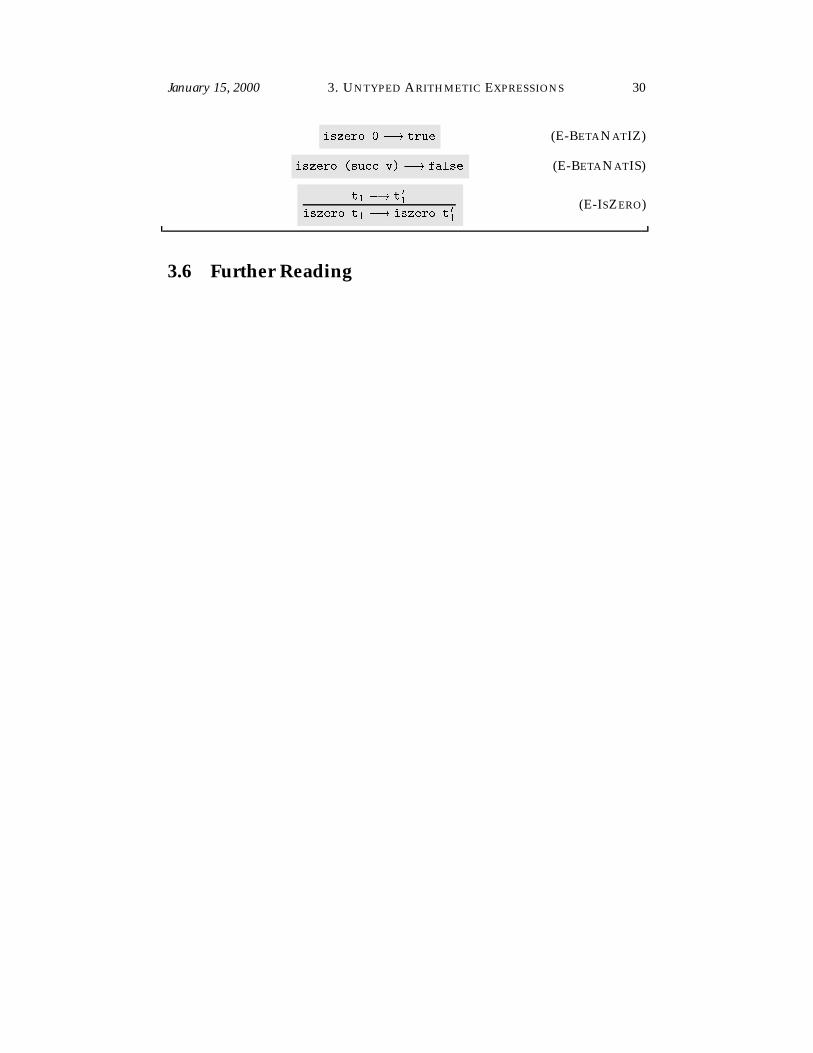
iszero 0 �! true (E-BETANATIZ)

iszero (succ v) �! false (E-BETANATIS)

t1 �! t 01iszero t1 �! iszero t 01

(E-ISZERO)

3.6 Further Reading

Chapter 4

The Untyped Lambda-Calculus

There may, indeed, be other applications of the system than its use as a logic.— Alonzo Church, 1932

In the mid 1960s, Peter Landin observed that a complex programming lan-guage can often be understood very cleanly by formulating it as a tiny “core cal-culus” capturing its essential mechanisms, together with a collection of conve-nient “derived forms” whose behavior is understood by translating them into thecore [Lan64, Lan65, Lan66] (also cf. [Ten81]). The core language used by Landinwas the lambda-calculus, a formal system in which all computation is reducedto the basic operations of function definition and application. Since the 60s, thelambda-calculus has seen widespread use in the specification of programming lan-guage features, language design and implementation, and the study of type sys-tems. Its importance arises from the fact that it can be viewed simultaneously as asimple programming language in which computations can be described and as amathematical object about which rigorous statements can be proved.

The lambda-calculus is just one of a large number of core calculi that have beenused for these purposes. For example, the pi-calculus of Robin Milner, JoachimParrow, and David Walker [MPW92, Mil91] has become a popular core languagefor defining the semantics of message-based concurrent languages, while MartınAbadi and Luca Cardelli’s object calculus [AC96] distills the core features of manyobject-oriented languages. The concepts and techniques we will develop for thelambda-calculus can, in most cases, be transferred quite directly to other calculi.

The lambda-calculus can be enriched in a variety of ways. First, it is often con-venient to add special concrete syntax for features like tuples and records whosebehavior can already be simulated in the core language. More interestingly, wemay want to provide more complex features such as mutable reference cells ornonlocal exception handling, which can be modeled in the core language only viarather heavy translations. Such extensions make the calculus look more like a full-

31

January 15, 2000 4. THE UNTYPED LAMBDA-CALCULUS 32

blown high-level programming language in its own right, and lead eventually tolanguages such as ML [GMW79, MTH90, WAL+89, MTHM97] and Scheme [SJ75,KCR98]. As we shall see, extensions to the core language often involve extensionsto the type system as well.

This chapter reviews the definition and some basic properties of the pure oruntyped lambda-calculus.

4.1 Basics

Procedural abstraction is a key feature of most programming languages. Instead ofwriting the same calculation over and over, we write a procedure or function thatperforms the calculation abstractly, in terms of one or more named parameters; wethen instantiate this function as needed, providing values for the parameters ineach case. For example, it is second nature for a programmer to take a long andrepetitive expression like

(5*4*3*2*1) + (7*6*5*4*3*2*1) - (3*2*1)

and rewrite it as

factorial(5)+factorial(7)-factorial(3),

where:

factorial(n) = if n=0 then 1 else n * factorial(n-1)

For each nonnegative number n, instantiating the function factorial with the ar-gument n yields a number, the factorial of n, as result. Writing “�n. ...” as ashorthand for “the function that, for each n, yields...,” we can restate the definitionof factorial as:

factorial = �n. if n=0 then 1 else n * factorial(n-1)

Then factorial(0) means “the function ‘�n. if n=0 then 1 else ...’ appliedto the argument 0,” that is, “the value that results when the bound variable n

in the function body ‘�n. if n=0 then 1 else ...’ is replaced by 0,” that is“if 0=0 then 1 else ...,” that is, 1.

In the 1930s, Alonzo Church invented a mathematical system called the lambda-calculus (or �-calculus) that embodies this kind of function definition and appli-cation in a pure form [Chu36, Chu41]. In the lambda-calculus everything is a func-tion: the arguments accepted by functions are themselves functions and the resultreturned by a function is another function.


Syntax

The syntax of the lambda-calculus comprises three kinds of terms. A variable x

by itself is a lambda-term; the application of a lambda-term t1 to another lambda-term t2, written t1 t2, is a lambda-term; and the abstraction of a variable x froma lambda-term t1, written �x. t1, is a lambda-term. These forms are summarizedin the following abstract grammar:

t ::= (terms...)x variable�x.t abstractiont t application

The letters s, t, and u (with or without subscripts) are used throughout to standfor arbitrary lambda-terms, while x, y, and z are used to stand for arbitrary vari-able names. We call s, t, u, x, y, and z metavariables: they are “variables” in thesense that they stand for terms of the lambda-calculus, and “meta” in the sense thatthey are part of the metalanguage (i.e. English plus ordinary mathematical nota-tions) in which an object language, the lambda-calculus, is being discussed. Sincethe set of short names is limited, we will also sometimes use x, y, etc. as object-language variables, but the context of the discussion will always make it clearwhich is which. For example, in a statement like “The term (�x. �y. x (y x))

has the form (�z. s), where z = x and s = �y. x (y x),” the names z and s aremetavariables, whereas x and y are object-language variables. A complete sum-mary of metavariable conventions appears in Appendix B.

The words “lambda-term” (or just “term”) and “lambda-expression” are oftenused as synonyms.

Note that what we’ve defined is only the abstract syntax of lambda-terms. In afull-scale programming language, we would also need to address concrete syntaxissues of lexing, parsing, operator precedence, etc. For present purposes, though, itis better to avoid such issues by concentrating on the abstract syntax, using paren-theses informally as necessary to clarify the tree structure of examples. Applicationis taken to “associate to the left”—that is, t s u is considered the same as (t s) u.Also, the bodies of abstractions are assumed to extend as far to the right as possi-ble, so that writing �m. �n. m n m is the same as writing �x. (�y. (x y) x).

The variable x is said to be bound in the body t of the abstraction �x.t. Con-versely, we say that a variable x is free in a term s if x appears at some position ins where it is not bound by an enclosing abstraction on x. For example, x is free inx y and �y. x y, but not in �x.x or �z. �x. �y. x (y z).

A term with no free variables is said to be closed; closed terms are also some-times called combinators. The simplest combinator is called the identity function:

id = �x.x;


Operational Semantics

In its pure form, the lambda-calculus has no built-in constants or operators—nonumbers, arithmetic operations, records, loops, sequencing, I/O, etc. The solemeans by which terms “compute” is the application of functions to arguments,which is captured in the following evaluation rule, traditionally called beta-reduction.

(�x.t12) v2 �! fx 7! v2gt12 (E-BETA)This rule says that an application of the form (�x.t1) v2 (where the argumenthas already been evaluated to a value), is evaluated by substituting the argumentv2 for the bound variable x in the body t1. For example, (�x.x) y evaluates to y

and (�x. x y) (u r) evaluates to u r y, while (�x.�y.x) z w evaluates (by theunderlined redex) to (�y.z) w, which further evaluates to z.

4.2 Programming in the Lambda-Calculus

The lambda-calculus is much more powerful than its tiny definition might suggest.For example, there is no built-in provision for multi-argument functions, but it iseasy to achieve the same effect using higher-order functions that yield functionsas results.

Suppose that s is a term involving two free variables x and y and we wantto write a function f that, for each pair (p,q) of arguments, yields the result ofsubstituting p for x and q for y in s. Instead of writing f = �(x,y).s, as we mightin a higher-level programming language, we write f = �x.�y.s. That is, f is afunction that, given a value p for x, yields a function that, given a value q for y,yields the desired result. We then apply f to its arguments one at a time, writingf p q, which reduces to (�y.fp 7! xgs) q and then to fq 7! ygfp 7! xgs. Thistransformation of multi-argument functions into higher-order functions is oftencalled Currying after its popularizer, Haskell Curry. (It was actually invented bySchonfinkel, but the term “Schonfinkeling” has not caught on.)

Another common language feature that can easily be encoded in the lambda-calculus is boolean values and conditionals. Define the terms tru and fls as fol-lows:

tru = �t. �f. t;

fls = �t. �f. f;

The only way to “interact” with combinators is by applying them to otherterms. For example, we can use application to define a combinator test withthe property that test b m n reduces to m when b = tru and reduces to q whenb = fls.

test = �l. �m. �n. l m n;


The test combinator does not actually do much: (test b m n) just reduces to(b m n). In effect, the boolean value b itself is the conditional: it takes two argu-ments and chooses the first (if it is tru) or the second (if it is fls). For example, theterm (test tru m n) reduces as follows:

test tru m n

= (�l. �m. �n. l m n) tru m n by definition�! (�m. �n. tru m n) m n reducing the underlined redex�! (�n. tru m n) n reducing the underlined redex�! tru m n reducing the underlined redex= (�t.�f.t) m n by definition�! (�f. m) n reducing the underlined redex�! m reducing the underlined redex

We can also write boolean operators like logical conjunction as functions:

and = �b. �c. b c fls;

That is, and is a function that, given two boolean arguments b and c, returns c if bis tru or fls if b is fls; thus and b c yields tru if both b and c are tru and fls ifeither b or c is fls.

and tru tru;

I (�t. �f. t)

and tru fls;

I (�t. �f. f)

and fls tru;

I (�t. �f. f)

and fls fls;

I (�t. �f. f)

4.2.1 Exercise: Define logical or and not functions. 2

Using booleans, we can encode pairs of values as lambda-terms. Define:

pair = �f.�s.�b. b f s;

fst = �p. p tru;

snd = �p. p fls;

That is, pair m n is a function that, when applied to a boolean b, applies b to m

and n. By the definition of booleans, this application yields m if b is tru and n if b isfls, so the first and second projection functions fst and snd can be implemented


simply by supplying the appropriate boolean. To check that fst (pair m n) �!�

m, calculate as follows:

fst (pair m n)

= fst ((�f. �s. �b. b f s) m n) by definition�! fst ((�s. �b. b m s) n) reducing the underlined redex�! fst (�b. b m n) reducing the underlined redex= (�p. p tru) (�b. b m n) by definition

�! (�b. b m n) tru reducing the underlined redex�! tru m n reducing the underlined redex�!� m as before.

The encoding of numbers as lambda-terms is only slightly more intricate thanwhat we have just seen. Define the Church numerals c0, c1, c2, etc., as follows:

c0 = �s. �z. z;

c1 = �s. �z. s z;

c2 = �s. �z. s (s z);

c3 = �s. �z. s (s (s z));

c4 = �s. �z. s (s (s (s z)));

etc.

That is, each number n is represented by a combinator cn that takes two argu-ments, z and s (for “zero” and “successor”), and applies s, n times, to z. As withbooleans and pairs, this encoding makes numbers into active entities: the numbern is represented by a function that does something n times—a kind of active unarynumeral.

We can define some common arithmetic operations on Church numerals as fol-lows:

plus = �m. �n. �s. �z. m s (n s z);

times = �m. �n. m (plus n) c0;

Here, plus is a combinator that takes two Church numerals, m and n, as arguments,and yields another Church numeral—i.e., a function that accepts arguments z ands, applies s iterated n times to z (by passing s and z as arguments to n), and thenapplies s iterated m more times to the result.

4.2.2 Exercise: Verify that (plus c2 c1) !� c3. 2

The definition of times uses another trick: since plus takes its arguments one at atime, applying it to just one argument n yields the function that adds n to whateverargument it is given. Passing this function as the second argument to m and c0 asthe first argument means “apply the function that adds n to its argument, iteratedm times, to zero,” i.e., “add together m copies of n.”

4.2.3 Exercise [Recommended]: Define a similar term for calculating the successorof a number. (Solution on page 254.) 2


4.2.4 Exercise: Define a similar term for raising one number to the power of an-other. 2

To test whether a Church numeral is zero, we must apply it to a pair of termszz and ss such that applying ss to zz one or more times yields fls, while notapplying it at all yields tru. Clearly, we should take zz to be just tru. For ss, weuse a function that throws away its argument and always returns fls.

iszro = �m. m (�x. fls) tru;

Surprisingly, it is quite a bit more difficult to subtract using Church numerals. Itcan be done using the following rather tricky “predecessor function,” which, givenc0 as argument, returns c0 and, given ci+1, returns ci:

zz = pair c0 c0;

ss = �p. pair (snd p) (plus c1 (snd p));

prd = �m. fst (m ss zz);

This definition works by using m as a function to apply m copies of the functionss to the starting value zz. Each copy of ss takes a pair of numerals pair ci cjas its argument and yields (pair cj cj+1) as its result. So applying ssm times to(pair c0 c0) yields (pair c0 c0) when m = 0 and (pair cm-1 cm) when m ispositive. In both cases, the predecessor of m is found in the first component.

4.2.5 Exercise:

1. Use prd to define a subtraction function.

2. How many steps of evaluation (as a function of n) are required to calculatethe result of (prd cn)? 2

4.2.6 Exercise: Write a function equal that tests two numbers for equality and re-turns a boolean. For example,

equal c3 c3;

I (�t. �f. t)

equal c3 c2;

I (�t. �f. f)

(Solution on page 254.) 2

Other common datatypes like lists, trees, arrays, and variant records can be en-coded using similar techniques. Of course, in most programming languages basedon the lambda-calculus, such basic data types are added as primitive constants,rather than being encoded.


4.2.7 Exercise [Recommended]: Build an encoding of lists in the pure lambda-calculus by defining a constant nil (the empty list) and operations cons (for con-structing a list from a new head element and an old list), head and tail (for ex-tracting the parts of a list), and isnull (for testing whether a list is empty).

One straightforward way to do this is to generalize the encoding of numbers asfollows. A list is represented by a function that takes two arguments, hh and tt. Ifthe list is empty, this function simply returns tt. On the other hand, if the list hashead h and tail t, the function calls hh, passing it h and (t hh tt) as parameters.(In other words, a list is represented by its own fold function.)

Can you think of any different ways of encoding lists? (Solution on page 254.)2

Recall that a term that cannot take a step under the evaluation relation is said tobe in normal form. Interestingly, in the untyped lambda-calculus, not every termcan be evaluated to a normal form. For example, the divergent combinator

omega = (�x. x x) (�x. x x);

can never be reduced to a value. It contains just one redex, and reducing this redexyields exactly omega again! Terms with no normal form are sometimes said todiverge.

The omega combinator has a useful generalization called the fixed-point com-binator (or Y-combinator), which can be used to define recursive functions suchas factorial.

fixpoint = �f. (�x. f (�y. (x x) y))

(�x. f (�y. (x x) y));

The crucial property of fixpoint is that fixpoint ff has the same behavior asff (fixpoint ff) for any term ff.

(Note that this is a call-by-value fixed point combinator, since we using a call-by-value reduction strategy. The simpler call-by-name fixed point combinator

fixpointn = �f. (�x. f (x x))

(�x. f (x x));

is useless in a call-by-value setting, since an expression like fixpointn ff alwaysdiverges, no matter what ff is.)

Now, suppose we want to write a recursive function definition of the formff = hbody containing ffi—i.e., we want to write a definition where the term onthe right-hand side of the = uses the very function that we are defining, as in thedefinition of factorial on page 32. The intention is that the recursive definitionshould be “unrolled” at the point where it occurs; for example, the definition offactorial would intuitively be:

if n=0 then 1

else n * (if n-1=0 then 1

else (n-1) * (if (n-2)=0 then 1

else (n-2) * ...))


This effect can be achieved using fixpoint by defining gg = �f.hbody containing fiand ff = fixpoint gg. For example, we can define the factorial function by

ff = �f. �n.

test

(iszro n) (�x. c1) (�x. (times n (f (prd n)))) c0;

factorial = fixpoint ff;

We then have:

equal (factorial c3) c6;

I (�t. �f. t)

4.2.8 Exercise [Recommended]: Use the fixpoint combinator and the encodingof lists from Exercise 4.2.7 to write a function that sums lists of church numerals.(Solution on page 254.) 2

4.3 Is the Lambda-Calculus a Programming Language?

4.4 Formalities

As we did in Chapter 3, we must now consider the syntax and operational seman-tics of the lambda-calculus in a little more detail. Most of the structure we need isclosely analogous to what we saw there. However, the operation of substituting aterm for a variable involves some surprising subtleties.

Syntax

As in Chapter 3, the abstract grammar defining terms should be read as shorthandfor the union of an inductively defined family of sets of abstract syntax trees. Todefine it precisely, we begin with some set V of variable names.

4.4.1 Definition [Terms]: The set of terms is the smallest set T such that

1. x 2 T for every x 2 V ;

2. if t1 2 T and x is a variable name, then �x.t1 2 T ;

3. if t1 2 T and t2 2 T , then (t1 t2) 2 T . 2

The size of a term t can be defined exactly as we did for arithmetic expressionsin Definition 3.2.7. More interestingly, we can give a simple inductive definition ofthe set of variables appearing “free” in a lambda-term.


4.4.2 Definition: The set of free variables of a term t, written FV(t), is defined asfollows:

FV(x) = fxg

FV(�x.t1) = FV(t1) n fxg

FV(t1 t2) = FV(t1) [ FV(t2) 2

Here is an inductive proof of a simple fact relating the definitions of size andfree variables, analogous to Lemma 3.2.8 in the previous chapter.

4.4.3 Lemma: The number of distinct free variables in a term t is always smallerthan the size of t (in symbols: jFV(t)j � size(t)). 2

Proof: By induction on the size of t. (That is, assuming the desired property forall terms smaller than t, we must prove it for t itself; if we can do this, we mayconclude that the property holds for all t.) There are three cases to consider:Case: t = x

Immediate: jFV(t)j = jfxgj = 1 = size(t).Case: t = �x.t1

By the induction hypothesis, jFV(t1)j � size(t1). We now calculate as follows:jFV(t)j = jFV(t1) n fxgj � jFV(t1)j � size(t1) < size(t).Case: t = t1 t2

By the induction hypothesis, jFV(t1)j � size(t1) and jFV(t2)j � size(t2). We nowcalculate as follows: jFV(t)j = jFV(t1) [ FV(t2)j � jFV(t1)j+ jFV(t2)j � size(t1) +size(t2) < size(t). 2

Substitution

Dealing carefully with the operation of substitution requires some work. We’lltake it in two large steps. First (in this section), we’ll discuss the basic issues, iden-tify some traps for the unwary, and come up with a definition of substitution thatis precise enough for most purposes. In Section 5.1 we’ll go the rest of the way,defining a more refined “nameless” presentation of terms on which substitutionis completely formal (and, in particular, suitable for implementation). The reasonfor presenting both is that the nameless formulation becomes too fiddly to use allthe time. Having worked it out in detail, we will return to the more comfortable,slightly informal presentation developed in this section, regarding it as a conve-nient shorthand for the other.

It is instructive to arrive at the correct definition of substitution via a couple ofwrong attempts. First off, let’s try the most naive possible recursive definition:

fx 7! sgx = s

fx 7! sgy = y if x 6= y

fx 7! sg(�y.t1) = �y. fx 7! sgt1fx 7! sg(t1 t2) = fx 7! sgt1 fx 7! sgt2


This definition works fine for most examples. For instance, it gives

fx 7! (�z. z w)g(�y. x) = (�y.�z. z w);

which is fine. However, if we are unlucky with our choice of bound variablenames, the definition breaks down. For example:

fx 7! yg(�x.x) = �x.y

This conflicts with the basic intuition about functional abstractions that the alpha-betic names of bound variables do not matter—the identity function is exactly the samewhether we write it �x.x or �y.y or �franz.franz. If these do not behave exactlythe same under substitution, then they will not behave the same under reductioneither, which seems wrong.

Clearly, the first mistake that we’ve made in the naive definition of substitutionis that we have not distinguished between free occurrences of a variable x in aterm t (which should get replaced during substitution) and bound ones, whichshould not. When we reach an abstraction binding the name x inside of t, thesubstitution operation should stop. This leads to the next attempt at a definition ofsubstitution:

fx 7! sgx = s

fx 7! sgy = y if y 6= x

fx 7! sg(�y.t1) =

��y. t1 if y = x

�y. fx 7! sgt1 if y 6= x

fx 7! sg(t1 t2) = fx 7! sgt1 fx 7! sgt2

This is better, but it is still not quite right. For example, consider what happenswhen we substitute the term z for the variable x in the term �z.x:

fx 7! zg(�z.x) = �z.z

This time, we have made essentially the opposite mistake as in the previous un-fortunate example: we’ve turned the constant function �z.x into the identity func-tion! Again, this occurred only because we happened to choose z as the name ofthe bound variable in the constant function, so something is clearly still wrong.

This phenomenon of free variables in a term s becoming bound when s isnaively substituted into a term t containing variable binders is called variablecapture. To avoid it, we need to make sure that the bound variable names of tkept distinct from the free variable names of s. A substitution operation that doesthis correctly is called capture-avoiding substitution. This is almost always whatis meant by the unqualified term “substitution.” We can achieve this by addinganother side condition to the second clause of the abstraction case:

fx 7! sgx = s


fx 7! sg(�y.t1) =

��y. t1 if y = x

�y. fx 7! sgt1 if y 6= x and y =2 FV(s)

fx 7! sg(t1 t2) = fx 7! sgt1 fx 7! sgt2


We are almost there: this definition of substitution does the right thing when itdoes anything at all. The problem now is that our last fix has changed substitutioninto a partial operation. For example, the new definition does not give any resultat all for fx 7! y zg(�y. x y): the bound variable y of the term being substitutedinto is not equal to x, but it does appear free in (y z), so none of the clauses of thedefinition apply.

One common fix for this last problem in the type systems and lambda-calculusliterature is to work with terms “up to renaming of bound variables” (or “up toalpha-conversion”):

4.4.4 Convention: Terms that differ only in the names of bound variables are in-terchangeable in all contexts. 2

What this means in practice is that the name of any bound variable can bechanged to another name (consistently making the same change in the body), atany point where this is convenient. For example, if we want to calculate fx 7!y zg(�y. x y), we first rewrite (�y. x y) as, say, (�w. x w). We then calculatefx 7! y zg(�w. x w), giving (�w. y z w). This renders the substitution operation“as good as total,” since whenever we find ourselves about to apply it to a collec-tion of arguments for which it is undefined, we can perform one or more steps ofrenaming as necessary, so that the side conditions are satisfied.

Indeed, having adopted this convention, we can formulate the definition ofsubstitution a little more tersely. The first clause for abstractions can be dropped,since we can always assume (renaming if necessary) that the bound variable y isdifferent from both x and the free variables of s. This yields the final form of thedefinition.

4.4.5 Definition [Substitution]:

fx 7! sgx = s


fx 7! sg(�y.t1) = �y. fx 7! sgt1 if y 6= x and y =2 FV(s)

fx 7! sg(t1 t2) = fx 7! sgt1 fx 7! sgt2 2

The convention about implicit renaming of bound variables is is easy to workwith, and its slight informality does not usually lead to trouble in practice. Weshall adopt it in most of what follows. However, it is also important to know howto formulate basic operations such as substitution with complete rigor, so that wehave a solid foundation to fall back on in case there is ever any question. We willsee one way to accomplish this in Section 5.1.

4.4.6 Exercise: Without looking forward to Section 5.1, can you think of any otherways in which the incomplete definition of substitution might be repaired to givea complete operation, without resorting to a convention about implicit renamingof bound variables? 2


Operational Semantics

4.4.7 Definition: The set of values is the subset of terms defined by the followingabstract grammar:

v ::= (values...)�x.t abstraction value

2

4.4.8 Definition: The one-step evaluation relation �! is the smallest relation con-taining all instances of the following rules:

(�x.t12) v2 �! fx 7! v2gt12 (E-BETA)

t1 �! t10

t1 t2 �! t 01 t2(E-APP1)

t2 �! t20

v1 t2 �! v1 t 02(E-APP2)

2

Summary

The foregoing definitions may be summarized compactly as follows.

� : Untyped lambda-calculus ! (untyped)

Syntax

t ::= (terms...)x variable�x.t abstractiont t application

v ::= (values...)�x.t abstraction value

Evaluation (t �! t 0)

(�x.t12) v2 �! fx 7! v2gt12 (E-BETA)

t1 �! t10

t1 t2 �! t 01 t2(E-APP1)

t2 �! t20

v1 t2 �! v1 t 02(E-APP2)


4.5 Further Reading

Information on the untyped lambda-calculus can be found in many places. Thefirst and best is Barendregt’s encyclopedic monograph, The Lambda Calculus [Bar84].Hindley and Seldin’s book [HS86] gives a more accessible treatment of some of thebasic material. Barendregt’s article in the Handbook of Theoretical Computer Sci-ence [Bar90] is a compact survey. Material on lambda-calculus can also be foundin many textbooks on functional programming languages (e.g. [AS85, FWH92,PJL92]) and programming language semantics (e.g.[Sch86, Gun92, Win93, Mit96]).

Chapter 5

Implementing theLambda-Calculus

Just because you’ve implemented something doesn’t mean you understand it.— Brian Cantwell Smith

5.1 Nameless Representation of Terms

In the previous chapter, we worked with terms “up to renaming of bound vari-ables.” This is fine for discussing basic concepts and for presenting proofs cleanly,but for building an implementation we need to choose a single concrete represen-tation for each term.

There are various ways to do this:

1. We can represent a variable occurrence as a string. This makes our concrete(“algorithmic”) representation close to the declarative one, but it means thatwe have to alpha-convert during substitution. This becomes quite tricky andit is easy to introduce subtle bugs.

2. We can replace the names chosen by the programmer with some canonicalnaming scheme.

3. We can avoid substitution altogether by introducing mechanisms like clo-sures.

We choose the second, using a well-known technique due to Nicolas de Bruijn [dB72].Making this choice will require some work now, but will save us a lot of trouble-some debugging when we come to implementing more complex systems.

45

January 15, 2000 5. IMPLEMENTING THE LAMBDA-CALCULUS 46

Syntax

De Bruijn’s idea was that we can represent terms more straightforwardly—thoughless readibly—by making variable occurrences point directly to their binders, ratherthan referring to them by name. This can be accomplished by replacing namedvariables by natural numbers, where the number k stands for “the variable boundby the k’th enclosing �” (starting from 0). For example, the ordinary term �x.x

corresponds to the nameless term �.0, while �x.�y. x (y x) is represented bythe nameless term �.�. 1 (0 1). Nameless terms are also sometimes called deBruijn terms, and the numeric variables in them are called de Bruijn indices. (Inpassing, a note on pronunciation: the closest English approximation to the secondsyllable in “de Bruijn” is “brown,” not “broyn.”)

5.1.1 Exercise [Quick check]: For each of the following combinators

c0 = �z. �s. z;

c2 = �z. �s. s (s z);

plus = �m. �n. �z. �s. m (n z s) s;

fixpoint = �f. (�x. f (x x)) (�x. f (x x));

foo = (�x. (�x. x)) (�x. x);

write down the corresponding nameless term. 2

Note that each (closed) ordinary term has just one de Bruijn representation,and that two ordinary terms are equivalent modulo renaming of bound variablesexactly when they have the same de Bruijn representation.

To deal with terms containing free variables, we need the idea of a namingcontext. For example, suppose we want to represent �x. y x as a nameless term.We know what to do with x, but we cannot see the binder for y, so it is not clearhow far out it might be and so we do not know what number to assign to it. Thesolution is to choose, once and for all, an assignment (called a naming context) ofde Bruijn indices to free variables, and use this assignment consistently when weneed to choose numbers for free variables. For example, suppose that we chooseto work under the following naming context:

� = x 7! 4

y 7! 3

z 7! 2

a 7! 1

b 7! 0

Then (x (y z)) would be represented as (4 (3 2)), while �x. y x would berepresented as �. 4 0 and �w.�a.x would be represented as �.�.6.

Actually, all we need to know about � is the order in which the variables appear.Instead of writing it in tabular form, as we did above, we will elide the numbersand write it as a sequence.


5.1.2 Definition: Suppose x0 through xn are variable names in V . The namingcontext � = xn; xn-1; : : :x1; x0 assigns to each xi the de Bruijn index i. Notethat the rightmost variable in the sequence is given the index 0. (This matches theway we count �s—from right to left—when converting a named term to namelessform.) We will write dom(�) for the set fx0; : : : ; xng of variable names mentionedin �. 2

Formally, we define the syntax of nameless terms almost exactly like the syntaxof ordinary terms (Definition 4.4.1). The only difference is that we need to keepcareful track of how many free variables each term may contain. That is, we dis-tinguish the sets of terms with no free variables (called the 0-terms), terms with atmost one free variable (1-terms), and so on.

5.1.3 Definition [Terms]: Let T be the smallest family of sets fT0; T1; T2; : : :g suchthat

1. k 2 Tn whenever 0 � k < n;

2. if t 2 Tn and n > 0, then �.t 2 Tn-1;

3. if t1 2 Tn and t2 2 Tn, then t1 t2 2 Tn.

The elements of each Tn are called n-terms. 2

Note that the elements of Tn are terms with at most free variables numberedbetween 0 and n - 1: a given element of Tn need not have free variables with allthese numbers, or indeed any free variables at all. If t is closed, for example, it willbe an element of Tn for every n.

Also, note that, strictly speaking, it does not make sense to speak of “somet 2 T ”—we always need to specify how many free variables t might have. Inpractice, though, we will often have some fixed naming context � in mind; we willthen abuse the notation slightly and write t 2 T to mean t 2 Tn, where n is thelength of �.

5.1.4 Exercise: Give an alternative construction of the sets of n-terms in the styleof 3.2.2, and show (as we did in Fact ??) that it is equivalent to the one above. 2

5.1.5 Exercise [Recommended]:

1. Define a function removenames that takes a naming context � and an ordinaryterm t (with FV(t) � dom(�)) and yields the corresponding nameless term.

2. Define a function restorenames that takes a nameless term t and a namingcontext � and produces an ordinary term. (To do this, you will need to “makeup” names for the variables bound by abstractions in t. You may assume thatthe set V of variable names is ordered, so that it makes sense to say “choosethe smallest variable name that is not already in dom(�).”)


This pair of functions should have the property that removenames�(restorenames�(t)) =t for any nameless term t, and similarly restorenames�(removenames�(t)) = t, upto renaming of bound variables, for any ordinary term t. 2

Shifting and Substitution

Before defining substitution on nameless terms, we need one auxiliary operationon terms, called “shifting,” which renumbers the indices of the free variables in aterm. When a substitution goes under a �-abstraction (as in fx 7! sg(�y.x)), thecontext in which the substitution is taking place becomes one variable longer thanthe original; we need to increment the indices of the free variables in s so that theykeep referring to the same names in the new context as they did before.

5.1.6 Definition [Shifting]: The d-place shift of a term t above cutoff c, written"dc (t), is defined as follows:

"dc (k) =

�k if k < c

k+ d if k � c"dc (�.t1) = �. "dc+1 (t1)"dc (t1 t2) = "dc (t1) "dc (t2)We will write "d (t) for "d0 (t). 2

5.1.7 Exercise [Quick check]:

1. What is "2 (�.�. 1 (0 2))?

2. What is "2 (�. 0 1 (�. 0 1 2))? 2

5.1.8 Exercise: Show that if t is an n-term, then "dc (t) is an (n+d)-term. 2

Now we are ready to define the substitution operator fj 7! sgt. At the end, wewill be most interested in substituting for the last variable in the context (i.e., j = 0),since that is the case we need in order to define the reduction relation. However,to substitute for variable 0 in a �-abstraction, we need to be able to substitute forvariable number 1 in the body. Thus, the definition of substitution must work onan arbitrary variable.

5.1.9 Definition [Substitution]: The substitution of a term s for variable number jin a term t, written fj 7! sgt, is defined as follows:

fj 7! sgk =

�s if k = j

k otherwisefj 7! sg(�.t1) = �. fj+ 1 7!"1 (s)gt1fj 7! sg(t1 t2) = fj 7! sgt1 fj 7! sgt2 2


5.1.10 Exercise [Quick check]: Convert the following substitution operations tonameless form (assuming the global context is � = a; b) and calculate their re-sults using the above definition. Do the answers make sense with respect to theoriginal definition of substitution on ordinary terms in Section 4.4?

� fb 7! ag (b (�x.�y.b))

� fb 7! ag (b (�x.�y.b))

� fb 7! (a (�z.a))g (b (�x.b)) 2

5.1.11 Exercise: Show that if s and t are n-terms and j � n, then fj 7! sgt is ann-term. 2

5.1.12 Exercise [Quick check]: Take a sheet of paper and, without looking at thedefinitions of substitution and shifting above, see if you can regenerate them. 2

5.1.13 Exercise [Recommended]: The definition of substitution on nameless termsshould agree with our informal definition of substitution on ordinary terms. Whattheorem would need to be proved to justify this correspondence rigorously? Forextra credit, prove it. (Solution on page 255.) 2

Evaluation

We can now define the evaluation relation on nameless terms.The beta-reduction rule is defined in terms of our new nameless substitution

operation. The only slightly subtle technical point is that reducing a redex “usesup” the bound variable—when we reduce (�x.t1) v2 to fx 7! v2gt1, the boundvariable x disappears in the process. Thus, we will need to renumber the variablesof the result of substitution to take into account the fact that x is no longer partof the context. Similarly, we need to shift the variables in v2 up by one beforesubstituting into t1 to take account of the fact that t1 is defined in a larger contextthan v2.

(�.t1) v2 �! "-1 (f0 7!"1 (v2)gt1) (E-BETA)The other rules are identical to what we had before.

5.2 A Concrete Realization


Syntax

type term =

TmVar of info * int * int

| TmAbs of info * string * term

| TmApp of info * term * term

let tmInfo = function

TmVar(fi,_,_) ! fi

| TmAbs(fi,_,_) ! fi

| TmApp(fi, _, _) ! fi

Shifting and Substitution

let tmmap onvar =

let rec walk c = function

TmVar(fi,x,n) ! onvar fi c x n

| TmAbs(fi,x,t1) ! TmAbs(fi, x, walk (c+1) t1)

| TmApp(fi,t1,t2) ! TmApp(fi, walk c t1, walk c t2)

in walk

let tmshifti d c t =

tmmap

(fun fi c x n ! if x>=c then TmVar(fi,x+d,n+d) else TmVar(fi,x,n+d))

c

t

let tmshift t d = tmshifti d 0 t

let tmsubsti s j t =

tmmap

(fun fi j x n ! if x=j then (tmshift s j) else TmVar(fi,x,n))

j

t

let tmsubst s t = tmsubsti s 0 t

let tmsubstsnip s t = tmshift (tmsubst (tmshift s 1) t) (-1)


Evaluation

let rec isval ctx = function

TmAbs(_,_,_) ! true

| _ ! false

let rec eval ctx t =

try let t' = eval1 ctx t

in eval ctx t'

with No ! t

5.3 Ordinary vs. Nameless Representations

Strictly speaking, having gone to the trouble of making all this so precise, weshould now continue through the rest of the material in the course using de Bruijnrepresentations consistently throughout. However, we will not do this, as it wouldmake the text essentially unreadable. Instead, we will adopt the following com-promise:

� In this chapter and in all the implementation sections to follow, we use deBruijn representations faithfully.

� In textual (and TeXtual) presentations of calculi, discussions, examples, andproofs, we will stick with the original presentation in terms of named vari-ables. However, we will always regard this as a convenient shorthand for anunderlying de Bruijn representation. For example, when we write

(�x.t11) t2 �! fx 7! t2gt11

we will actually mean:(�.t11) t2 �! "-1 (f0 7!"1 (t2)gt11)

In particular, this convention has the following consequences:

1. we always work “up to alpha-conversion,” ignoring the particular nameschosen for bound variables, and

2. whenever we mention a term, we will always (at least implicitly) havesome context in mind that imposes a numerical ordering on its free vari-able names.

Chapter 6

Typed Arithmetic Expressions

This and the following chapter are technically mostly complete but the text needs to beexpanded. The idea is that, as we did in the untyped case, we go through all the basic factsabout typed calculi in the very simple setting of just numbers and booleans, then redo it allfor the lambda-calculus.

6.1 Syntax

6.1.1 Definition: The set of types for arithmetic expressions contains just the sym-bols Bool and Nat:

T ::= (types...)Bool type of booleansNat type of natural numbers

The metavariables S, T, U, etc. range over types. 2

6.2 The Typing Relation

The type system for arithmetic expressions is defined by a set of rules assigningtypes to terms. We write “` t : T” to mean “term t has type T.”

For example, the fact that the term 0 has the type Nat is captured by the follow-ing axiom:

0 : Nat (T-ZERO)Similarly, the term succ t1 has type Nat as long as t1 has type Nat.

t1 : Nat

succ t1 : Nat(T-SUCC)

52

January 15, 2000 6. TYPED ARITHMETIC EXPRESSIONS 53

Likewise, pred yields a Nat when its argument has type Nat

t1 : Nat

pred t1 : Nat(T-PRED)

and iszero yields a Bool when its argument has type Nat:t1 : Nat

iszero t1 : Bool(T-ISZERO)

The boolean constants both have type Bool

true : Bool (T-TRUE)

false : Bool (T-FALSE)The only interesting typing rule is the one for if expressions:

t1 : Bool t2 : T t3 : T

if t1 then t2 else t3 : T(T-IF)

The metavariable T is used to indicate that the result of the if is the type of thethen- and else- branches, and that this may be any type (either Nat or Bool or,when we get to calculi with more interesting sets of types, any other type whatso-ever).

6.3 Properties of Typing and Reduction

Typing Derivations

Formally, the typing relation can be thought of as a simple logic for proving typingassertions (sometimes called typing judgements) of the form ` t : T, pronounced“the term t has the type T.” The provable statements of this logic are defined asfollows:

6.3.1 Definition: The typing relation is the least two-place relation containing allinstances of the axioms T-ZERO, T-TRUE, and T-FALSE and closed under all in-stances of the remaining rules. (In the literature on type systems, the symbol 2 isoften used instead of : for the typing relation.) 2

6.3.2 Definition: A typing derivation is a tree of instances of the typing rules.Each statement ` t : T in the typing relation is justified by a typing derivationwith conclusion ` t : T. We sometimes write D :: J to indicate that D is a deriva-tion tree with conclusion J . When D :: J for some D, we say that J is derivable.2

6.3.3 Theorem [Principle of induction on typing derivations]: Suppose that P issome predicate on typing statements. If we can show, for each typing derivationD :: J , that (P(J 0), for all D 0 :: J 0 with size(D 0) < size(D)) implies P(J ), then wemay conclude that P(J ) holds for every derivable typing statement. 2


Typechecking

6.3.4 Lemma [Inversion of the typing relation]:

1. If ` 0 : R, then R = Nat.

2. If ` succ t1 : R, then R = Nat and ` t1 : Nat.

3. If ` pred t1 : R, then R = Nat and ` t1 : Nat.

4. If ` iszero t1 : R, then R = Bool and ` t1 : Nat.

5. If ` true : R, then R = Bool.

6. If ` false : R, then R = Bool.

7. If � ` if t1 then t2 else t3 : R, then

� ` t1 : Bool

� ` t2 : R

� ` t3 : R:

The inversion lemma is sometimes called the generation lemma for the typing re-lation, since, given a valid typing statement, it shows how proofs of this statementmight have been generated. 2

Proof: Immediate from the definition of the typing relation. 2

6.3.5 Theorem [Uniqueness of Types]: Each term t has at most one type. That is,if t is typeable, then its type is unique. Moreover, there is just one derivation ofthis typing built from the inference rules of Definition 6.3.1. 2

Proof: Exercise. 2

Safety = Preservation + Progress

The most important property of this type system (or any other) is soundness: well-typed programs do not “go wrong.” A simple way of formalizing this fact is theobservation that well-typed programs can only reduce to well-typed programs—that is, a well-typed program can never reach an ill-typed state at run-time.

6.3.6 Theorem [Preservation of types during evaluation]: If ` t : T and t �! �

t 0, then ` t 0 : T. 2

Proof: Exercise. 2


The preservation theorem is often called “subject reduction” (or “subject evalu-ation”) in the literature—the intuition being that a typing statement ` t : T can bethought of as a sentence: “t has type T.” The term t is the subject of this sentence,and the subject reduction property then says that the truth of the sentence is stableunder reduction of the subject.

Recall (from Definition3.2.16) that a “stuck” term is one that is in normal formbut not a value.

6.3.7 Theorem [Progress]: If ` t : T, then either t is a value or there is some t 0

such that t �! t 0. 2

Proof: Exercise. 2

The combination of the latter property with the preservation theorem guar-antees that “well-typed terms never get stuck.” This combination of propertiescaptures what is usually thought of as “type safety” or “type soundness.”

6.3.8 Exercise [Recommended]: Having seen the “subject reduction” property, wemay wonder whether the opposite (“subject expansion”) property also holds. Is italways the case that, if t �!� t 0 and ` t 0 : T, then ` t : T? If so, prove it. If not,give a counterexample. (Solution on page 255.) 2

6.4 Implementation

type ty =

TyBool

| TyNat

let rec tyeqv tyS tyT =

match (tyS,tyT) with

(TyBool,TyBool) ! true

| (TyNat,TyNat) ! true

| _ ! false

val error : info ! string ! 'a

let rec typeof t =

match t with

TmTrue(fi) !

TyBool

| TmFalse(fi) !

TyBool

| TmIf(fi,s1,s2,s3) !

if tyeqv (typeof s1) TyBool then

let tyS = typeof s2 in


if tyeqv tyS (typeof s3) then tyS

else error fi "arms of conditional have different types"

else error fi "guard of conditional not a boolean"

| TmZero(fi) !

TyNat

| TmSucc(fi,t1) !

if tyeqv (typeof t1) TyNat then TyNat

else error fi "argument of succ is not a number"

| TmPred(fi,t1) !

if tyeqv (typeof t1) TyNat then TyNat

else error fi "argument of pred is not a number"

| TmIsZero(fi,t1) !

if tyeqv (typeof t1) TyNat then TyBool

else error fi "argument of iszero is not a number"

6.5 Summary

Typing rules for booleans B (typed)

New syntactic forms

T ::= ... (types...)Bool type of booleans

New typing rules (t : T)

true : Bool (T-TRUE)

false : Bool (T-FALSE)

t1 : Bool t2 : T t3 : T

if t1 then t2 else t3 : T(T-IF)

Typing rules for numbers B N (typed)

New syntactic forms

T ::= ... (types...)Nat type of natural numbers

New typing rules (t : T)

0 : Nat (T-ZERO)


t1 : Nat

succ t1 : Nat(T-SUCC)

t1 : Nat

pred t1 : Nat(T-PRED)

t1 : Nat

iszero t1 : Bool(T-ISZERO)

Chapter 7

Simply TypedLambda-Calculus

This chapter introduces the most elementary member of the family of typed lan-guages that we shall be studying for the rest of the course: the simply typedlambda-calculus of Church [Chu40] and Curry [CF58].

7.1 Syntax

7.1.1 Definition: The set of simple types over the atomic type Bool (for brevity,we omit natural numbers) is generated by the following grammar:

T ::= (types...)T!T type of functionsBool type of booleans

The type constructor! is right-associative: S!T!U stands for S!(T!U). 2

7.1.2 Definition: The abstract syntax of simply typed lambda-terms (with booleansand conditional) is defined by the following grammar:

t ::= (terms...)x variable�x:T.t abstractiont t applicationtrue constant truefalse constant falseif t then t else t conditional

2

58

January 15, 2000 7. SIMPLY TYPED LAMBDA-CALCULUS 59

In the literature on type systems, two different presentation styles are com-monly used:

� In implicitly typed (or, for historical reasons, Curry-style) systems, the pure(untyped) lambda-calculus is used as the term language. The typing rulesdefine a relation between untyped terms and the types that classify them.

� In explicitly typed (or Church-style) systems, the term language itself is re-fined so that terms carry some type information within them; for example,the bound variables in function abstractions are always annotated with thetype of the expected parameter. The type system relates typed terms andtheir types.

To a large degree, the choice is a matter of taste, though explicitly typed systemsgenerally pose fewer algorithmic problems for typecheckers. We will adopt anexplicitly typed presentation throughout.

7.2 The Typing Relation

In order to assign a type to an abstraction like �x:T2.t1, we need to know whatwill happen later when it is applied to some argument t2. The annotation on thebound variable tells us that we may assume that the argument will be of type T2.In other words, the type of the result will be just the type of t1, where occurrencesof x in t1 are assumed to denote terms of type T2. This intuition is captured by thefollowing rule:

x:T1 ` t2 : T2

` �x:T1.t2 : T1!T2(T-ABS)

Since, in general, function abstractions can be nested, typing assertions actuallyhave the form � ` t : T, pronounced “term t has type T under the assumptions �about the types of its free variables.” Formally, the typing context � is just a list ofvariables and their types, and the “comma” operator extends � by concatenating anew binding on the right. To avoid confusion between the new binding and anybindings that may already appear in �, we require that the name x be chosen sothat it does not already appear in dom(�). (As usual, this condition can always besatisfied by renaming the bound variable if necessary.) � can thus be thought ofas a finite function from variables to their types. Following this intuition, we willwrite dom(�) for the set of variables bound by � and �(x) for the type T associatedwith x in �.

So the rule for typing abstractions actually has the general form

�; x:T1 ` t2 : T2

� ` �x:T1.t2 : T1!T2(T-ABS)

where the premise adds one more assumption to those in the conclusion.


The typing rule for variables follows immediately from this discussion. A vari-able has whatever type we are currently assuming it to have:

x:T 2 �

� ` x : T(T-VAR)

Next, we need a rule for application:� ` t1 : T11!T12 � ` t2 : T11

� ` t1 t2 : T12(T-APP)

In English: If t1 evaluates to a function mapping arguments in T2 to results in T1(under the assumption that the terms represented by its free variables yield resultsof the types associated to them by �), and if t2 evaluates to a result in T2, then theresult of applying t1 to t2 will be a value of type T1.

We have now given typing rules for each of the individual constructs in oursimple language. To assign types to whole programs, we combine these rulesinto derivation trees. For example, here is a derivation tree showing that the term(�x:Bool.x) true has type Bool in the empty context:

T-VARx:Bool ` x : Bool

T-ABS` �x:Bool.x : Bool!Bool

T-TRUE` true : Bool

T-APP` (�x:Bool.x) true : Bool

7.2.1 Exercise [Quick check]: Show (by exhibiting derivation trees) that the fol-lowing terms have the indicated types in the given contexts:

1. f:Bool!Bool ` f (if false then true else false) : Bool

2. f:Bool!Bool ` �x:Bool. f (if x then false else x) : Bool!Bool 2

7.2.2 Exercise [Quick check]: Find a context � under which the term f x y hastype Bool. Can you give a simple description of the set of all such contexts? 2

It is interesting to note that, in the above discussion, the “!” type constructorcomes with typing rules of two kinds:

1. an introduction rule describing how elements of the type can becreated, and

2. an elimination rule describing how elements of the type can beused.

This terminology, which arises from connections between type theory and logic,is frequently useful in discussing type systems. When we come to consider morecomplex systems later in the course, we’ll see a similar pattern of linked introduc-tion and elimination rules being repeated for each type constructor we consider.

7.2.3 Exercise [Quick check]: Which of the rules for the type Bool are introductionrules and which are elimination rules? (Solution on page 255.) 2


7.3 Summary

We have been discussing the simply typed lambda-calculus with booleans andconditionals, �!B . In later chapters, we are going to want to extend the simplytyped lambda-calculus with many other base types, in addition to or instead ofbooleans. We therefore split the formal summary of the system into two pieces: thepure simply typed lambda calculus �!, with no base types at all, and a separateextension with booleans.

�! : Simply typed lambda-calculus ! (typed)

Syntax

t ::= (terms...)x variable�x :T .t abstractiont t application

v ::= (values...)�x :T .t abstraction value

T ::= (types...)T!T type of functions

� ::= (contexts...); empty context�; x:T term variable binding

Evaluation (t �! t 0)(�x :T11 .t12) v2 �! fx 7! v2gt12 (E-BETA)

t1 �! t10

t1 t2 �! t 01 t2(E-APP1)

t2 �! t20

v1 t2 �! v1 t 02(E-APP2)

Typing ( � ` t : T)

x:T 2 �

� ` x : T(T-VAR)

�; x:T1 ` t2 : T2

� ` �x:T1.t2 : T1!T2(T-ABS)


� ` t1 : T11!T12 � ` t2 : T11

� ` t1 t2 : T12(T-APP)

The highlighted areas here are used to mark material that is new with respect tothe untyped lambda-calculus—whole new rules as well as new bits that need to beadded to rules that we have already seen.

7.3.1 Exercise [Quick check]: The system �! by itself is actually trivial, in thesense that it has no well-typed programs at all. Why? (Solution on page 255.) 2

7.4 Properties of Typing and Reduction

Typechecking

As in Chapter 6, we need to develop a few basic lemmas before we can provetype soundness. Most of these are similar to what we saw before (just addingcontexts to the typing relation and adding appropriate clauses for �-terms. Theonly significant new requirement is a substitution principle for the typing relation(Lemma 7.4.9).

7.4.1 Lemma [Inversion of the typing relation]:

1. If � ` x : R, then x:R 2 �.

2. If � ` �x:T2. t1 : R2!R1, then R2 = T2 and �; x:T2 ` t1 : R1.

3. If � ` t1 t2 : R, then there is some type T2 such that � ` t1 : T2!R and� ` t2 : T2.

4. If � ` true : R, then R = Bool.

5. If � ` false : R, then R = Bool.

6. If � ` if t1 then t2 else t3 : R, then

� ` t1 : Bool

� ` t2 : R

� ` t3 : R: 2

Proof: Immediate from the definition of the typing relation. 2

7.4.2 Exercise [Easy]: Write out a typechecking algorithm for �! in pseudo-codeor a programming language of your choice. Compare your answer with the MLimplementation in Section 7.5. 2


In Section 7.1, we chose to use an explicitly typed presentation of the calculus,partly in order to simplify the algorithmic issues involved in typechecking. Thisinvolved adding type annotations to bound variables in function abstractions, butnowhere else. In what sense is this “enough”?

One answer is provided by the “uniqueness of types” theorem, the substanceof which is that well-typed terms are in one-to-one correspondence with the typingderivations that justify their well-typedness (in a given environment). The typingderivation can be recovered immediately from the term, and vice versa. In fact, thecorrespondence is so straightforward that, in a sense, there is little difference be-tween the term and the derivation. (For many of the type systems that we will see,this simple correspondence will not hold: there will be significant work involvedin showing that typing derivations can be recovered effectively from typed terms.)

7.4.3 Theorem [Uniqueness of Types]: In a given typing context �, a term t (withfree variables all in the domain of �) has at most one type. That is, if a term istypeable, then its type is unique. Moreover, there is just one derivation of thistyping built from the inference rules that generate the typing relation. 2

The proof of the uniqueness theorem is so direct that there is almost nothingto say. We present a few cases carefully just to illustrate the structure of proofs byinduction on typing derivations.

Proof: Suppose that � ` t : S and � ` t : T. We show, by induction on a deriva-tion of � ` t : T, that S = T.Case T-VAR: t = x

with x:T 2 �

By case (1) of the inversion lemma (7.4.1), the final rule in any derivation of � ` t :

S must also be T-VAR, and S = T.Case T-ABS: t = �y:T2.t1

T = T2!T1�; y:T2 ` t1 : T1

By case (2) of the inversion lemma, the final rule in any derivation of � ` t : S

must also be T-ABS, and this derivation must have a subderivation with conclu-sion �; y:T2 ` t1 : S1, with S = T2!S1. By the induction hypothesis (on thesubderivation with conclusion (�; y:T2 ` t1 : T1), we obtain S1 = T1, from whichS = T is immediate.Case T-APP, T-TRUE, T-FALSE, T-IF:Similar. 2

7.4.4 Exercise [Quick check]: Write out the case for T-APP. 2

7.4.5 Exercise [Recommended]: Is there any context � and type T such that � `x x : T? If so, give � and T and show a typing derivation for � ` x x : T; if not,prove it. 2


We shall sometimes need to talk about the types of subterms of well-typedterms. The following notation is useful for this purpose.

7.4.6 Definition: Suppose the term s is well typed with respect to the typing con-text �, and that r is some subterm of s. We write typeOf

�(r) for the type R such

that � 0 ` r : R, where � 0 is calculated by extending � with bindings correspondingto all of the function abstractions inside s under which r occurs. For example, ifs = �f:A!B. �g:A. f g and r = f g, then typeOf

�(r) = B. When (as in this chap-

ter) � is fixed for the whole discussion, we usually elide it, writing just typeOf(r).Note that R is unique, by Theorem 7.4.3. 2

We close this section with a couple of “structural lemmas” for the typing re-lation. These are not particularly interesting in themselves, but will permit us toperform some useful manipulations of typing derivations in later proofs.

7.4.7 Lemma [Permutation]: If � ` t : T and � is a permutation of �, then � ` t :

T. Moreover, the latter derivation has the same depth as the former. 2

Proof: Straightforward induction on typing derivations. 2

7.4.8 Lemma [Weakening]: If � ` t : T and x =2 dom(�), then �; x:S ` t : T.Moreover, the latter derivation has the same depth as the former. 2


Typing and Substitution

7.4.9 Lemma [Substitution]: If �; x:S ` t : T and � ` s : S, then � ` fx 7! sgt :

T. 2

7.4.10 Exercise [Recommended]: Prove the substitution lemma, using an induc-tion on the depth of typing derivations and Lemma 7.4.1. The full proof appearsin the solutions; try to write it out yourself before having a look at the answer.(Solution on page 255.) 2

Type Soundness

7.4.11 Theorem [Preservation of types during evaluation]: If � ` t : T and t �! �

t 0, then ` t 0 : T. 2

Proof: 2

7.4.12 Theorem [Progress]: Suppose t is closed and stuck. If ` t : T, then t is avalue. 2

Proof: Outline: first show that every closed value of type Bool is either true orfalse and every closed value of type S!T is a � abstraction. 2


7.5 Implementation

type ty =

TyArr of ty * ty

| TyBool

type term =


| TmAbs of info * string * ty * term


| TmTrue of info

| TmFalse of info

| TmIf of info * term * term * term

let rec tyeqv tyS tyT =


(TyArr(tyS1,tyS2),TyArr(tyT1,tyT2)) !

(tyeqv tyS1 tyT1) && (tyeqv tyS2 tyT2)

| (TyBool,TyBool) ! true

| _ ! false

let rec typeof ctx t =

match t with

TmVar(fi,i,_) !

gettype fi ctx i

| TmAbs(fi,x,tyS,t1) !

let ctx' = addbinding ctx x (VarBind(tyS)) in

let tyT = typeof ctx' t1 in

TyArr(tyS, tyshift tyT (-1))

| TmApp(fi,t1,t2) !

let tyT1 = typeof ctx t1 in


(match tyT1 with

TyArr(tyT11,tyT12) !

if tyeqv tyT2 tyT11 then tyT12

else error fi "parameter type mismatch"

| _ ! error fi "arrow type expected")

| TmTrue(fi) !

TyBool

| TmFalse(fi) !

TyBool


if tyeqv (typeof ctx s1) TyBool then

let tyS = typeof ctx s2 in

if tyeqv tyS (typeof ctx s3) then tyS

else error fi "arms of conditional have different types"



7.6 Further Reading

The untyped lambda-calculus was developed by Church and his co-workers in the1930s [Chu41]. The standard text for all aspects of the untyped lambda-calculus isBarendregt [Bar84]. Hindley and Seldin [HS86] is less comprehensive, but some-what more accessible. Barendregt’s article in the Handbook of Theoretical Com-puter Science [Bar90] is a compact survey.

The simply typed lambda-calculus is studied in Hindley and Seldin [HS86]and in even greater detail in Hindley’s more recent book [Hin97]. Material onboth typed and untyped lambda-calculus can also be found in many textbookson functional programming languages (e.g. [PJL92]) and programming languagesemantics (e.g.[Sch86, Gun92, Win93, Mit96]).

Chapter 8

Extensions

This chapter is just a sketch (but all the underlying implementations are finished, so itwon’t be too hard to fill in). It presents a bunch of familiar typing features and program-ming language constructs and shows how they fit into the framework we’ve built. Thereshould be lots of exercises.

8.1 Base Types

Base types ! B

New syntactic forms

T ::= ... (types...)B base type

8.2 Unit type

Unit type ! Unit

New syntactic forms

t ::= ... (terms...)unit constant unit

T ::= ... (types...)

67

January 15, 2000 8. EXTENSIONS 68

Unit unit type

New typing rules (� ` t : T)

� ` unit : Unit (T-UNIT)

Note: C and Java’s void type is a misnomer – what they really mean is Unit

8.3 Let bindings

Let binding ! let

New syntactic forms

t ::= ... (terms...)let x=t in t let binding


let x=v1 in t2 �! fx 7! v1gt2 (E-LETBETA)

t1 �! t10

let x=t1 in t2 �! let x=t 01 in t2(E-LET)


� ` t1 : T1 �; x:T1 ` t2 : T2

� ` let x=t1 in t2 : T2(T-LET)

8.3.1 Exercise [Recommended]: Add let bindings to the “simple” typecheckerimplementation. (Solution on page ??.) 2

8.4 Records and Tuples


Records and tuples ! fg

New syntactic forms

t ::= ... (terms...){li=ti

i21::n} recordt.l projection

v ::= ... (values...){li=vi

i21::n} record value

T ::= ... (types...){li:Ti

i21::n} type of records


{li=vii21::n}.li �! vi (E-RCDBETA)

t1 �! t 01t1.l �! t 01.l

(E-PROJ)

tj �! t 0j{li=vi

i21::n} �! {li=vii21::j-1,lj=t

0j,lk=tk

k2j+1::n}(E-RECORD)


for each i � ` ti : Ti

� ` {li=tii21::n} : {li:Ti

i21::n}(T-RCD)

� ` t : {li:Tii21::n}

� ` t.lj : Tj(T-PROJ)

New abbreviations

{...ti...}def= {...i=ti...}

{...Ti...}def= {...i:Ti...}

8.4.1 Exercise: In this presentation of records, the projection operation is used toextract the fields of a record one by one. Many high-level programming languagesprovide an alternative pattern matching syntax that extracts all the fields at thesame time, allowing many programs to be expressed more concisely. Patterns cantypically be nested, allowing parts to be extracted easily from complex nested datastructures.

For example, we can add a simple form of pattern matching to the untypedlambda calculus with records by adding a new syntactic category of patterns, plus


one new case (for the pattern matching construct itself) to the syntax of terms. Todefine the computation rule for pattern matching, we need an auxiliary “match-ing” function. Given a pattern and a term, the pattern matching function eitherfails (if the term does not match the pattern) or else yields a substitution that re-places variables appearing in the pattern with the corresponding subterms of thegiven term. Here is the formal definition of the calculus, highlighting differencesfrom the pure untyped lambda-calculus with records and ordinary let-binding:


Record patterns ! fg let pat (untyped)

New syntactic forms

p ::= :::

x variable pattern{li=pi

i21::n} record pattern

t ::= ... (terms...)let p =t in t pattern binding

Matching rules:

match(x; t) = fx 7! tg (M-VAR)

for each i match(pi; ti) = �i

match({li=pi i21::n}; {li=ti i21::n}) = �1 Æ � � � Æ �n(M-RCD)

New evaluation rules (t �! t 0)let p =v1 in t2 �! match(p; v1) t2 (E-LETBETA)

t1 �! t10

let p =t1 in t2 �! let p =t 01 in t2(E-LET)

New abbreviations

{...pi...}def= {...i=pi...}

Your job is to add types to this calculus, in the style of the simply typed lambda-calculus:

1. Give typing rules for the new constructs (making any changes to the syntaxyou feel are necessary in the process).

2. Sketch a proof of type preservation and progress for the whole calculus bystating the sequence of major lemmas needed to carry out the proof. (Youdo not need to show proofs, just statements of the required lemmas in thecorrect order.)



8.5 Variants

Variants ! <>

New syntactic forms

t ::= ... (terms...)<l=t> as T taggingcase t of ... | li=x)ti | ... case

T ::= ... (types...)<li:Ti

i21::n> type of variants


case <li=vi> as T of ...|li=x)ti|... �! fx 7! vigti (E-CASEBETA)

s1 �! s10

case s1 of ...|li=x)ti|... �! case s 01 of ...|li=x)ti|...(E-CASE)

ti �! ti0

<li=ti> as T �! <li=t0i> as T

(E-TAG)


for each i � ` ti : Ti

� ` <li=ti> as <li:Tii21::n> : <li:Ti

i21::n>(T-VARIANT)

� ` t0 : <li:Tii21::n>

for each i �; xi:Ti ` ti : T

� ` case t0 of ...|li=xi)ti|... : T(T-CASE)

Note that we syntactically allow the type label to be a non-variant type, but thetyping rule then excludes this case. This is just for brevity (and implementationflexibility, e.g. when we get to definitions).

8.6 General recursion


General recursion ! fix

New syntactic forms

t ::= ... (terms...)fix t fixed point of t


� ` t1 : T1!T1

� ` fix t1 : T1(T-FIX)

New abbreviations

letrec x=t1 in t2def= let x = fix (�x.t1) in t2

A corollary of the definability of fixed-point combinators at every type is thatevery type in this system is inhabited. For example, for each type T, the application(divergeT unit) has type T, where divergeT is defined like this:

divergeT = �_:Unit. fix (�x:T. x);

I T = Nat: *

divergeT : Unit ! T

8.7 Lists

Lists ! B List

New syntactic forms

t ::= ... (terms...)nil [T] empty listcons [T] t t list constructornull [T] t test for empty listhead [T] t head of a listtail [T] t tail of a list

v ::= ... (values...)nil [T] empty listcons [T] v v list constructor

T ::= ... (types...)List T type of lists



t1 �! t 01cons[T] t1 t2 �! cons[T] t 01 t2

(E-CONS1)

t2 �! t 02cons[T] v1 t2 �! cons[T] v 01 t2

(E-CONS2)

null[S] (nil[T]) �! true (E-NULLBETAT)

null[S] (cons[T] v1 v2) �! false (E-NULLBETAF)

t1 �! t 01null[T] t1 �! null[T] t 01

(E-NULL)

head[S] (cons[T] v1 v2) �! v1 (E-HEADBETA)

t1 �! t 01head[T] t1 �! head[T] t 01

(E-HEAD)

tail[S] (cons[T] v1 v2) �! v1 (E-TAILBETA)

t1 �! t 01tail[T] t1 �! tail[T] t 01

(E-TAIL)


� ` nil [T] : List T (T-NIL)

� ` t1 : T1 � ` t2 : List T1

� ` cons t1 t2 : List T1(T-CONS)

� ` t1 : List T1

� ` null t1 : Bool(T-NULL)

� ` t1 : List T1

� ` head t1 : T1(T-HEAD)

� ` t1 : List T1

� ` tail t1 : List T1(T-TAIL)


8.8 Lazy records and let-bindings

Lazy let bindings ! let lazy

New syntactic forms

t ::= ... (terms...)lazy let x=t in t lazy let binding


lazy let x=t1 in t2 �! fx 7! t1gt2 (E-LLETBETA)


� ` t1 : T1 �; x:T1 ` t2 : T2

� ` lazy let x=t1 in t2 : T2(T-LLET)

Lazy records ! fg lazy

New syntactic forms

t ::= ... (terms...)lazy {li=ti

i21::n} lazy record

v ::= ... (values...)lazy {li=ti

i21::n} lazy record value


(lazy {li=tii21::n}).li �! ti (E-LRCDBETA)


� ` i21::n ti : Ti

� ` lazy {li=tii21::n} : {li:Ti

i21::n}(T-LRCD)

Exercise: write down rules for lazy functions(These are used only in the advanced parts of the object examples.)

Chapter 9

References

This chapter is still very rough. The basic approach seems fine, but there’s a good deal ofwork to do on details.

References ! Unit :=

Syntax

t ::= (terms...)x variable�x:T.t abstractiont t applicationunit constant unitl store locationref t reference creation!t dereferencet:=t assignment

v ::= (values...)�x:T.t abstraction valuel store location

T ::= (types...)T!T type of functionsUnit unit typeRef T1 type of reference cells


76

January 15, 2000 9. REFERENCES 77

� ::= ; empty store�; l = t location binding

� ::= ; empty store typing�; l:T location typing

Evaluation (t j � �! t 0 j � 0 )

(�x :T11 .t12) v2 j � �! fx 7! v2gt12 j � (E-BETA)

t1 j � �! t10 j � 0

t1 t2 j � �! t 01 t2 j �0

(E-APP1)

t2 j � �! t20 j � 0

v1 t2 j � �! v1 t 02 j �0

(E-APP2)

l =2 dom(�)

ref v1 j � �! l j (�; l = v1)(E-REF)

t1 j � �! t10 j � 0

ref t1 j � �! ref t 01 j � 0(E-REF1)

�(l) = v

!l j � �! v j �(E-DEREF)

t1 j � �! t10 j � 0

!t1 j � �! !t 01 j �0 (E-DEREF1)

l:=v2 j � �! unit j fl 7! v2g� (E-ASSIGN)

t1 j � �! t10 j � 0

t1:=t2 j � �! t 01:=t2 j � 0(E-ASSIGN1)

t2 j � �! t20 j � 0

v1:=t2 j � �! v1:=t02 j � 0

(E-ASSIGN2)

Typing (� j � ` t : T)

x:T 2 �

� j � ` x : T(T-VAR)

�; x:T1 j � ` t2 : T2

� j � ` �x:T1.t2 : T1!T2(T-ABS)


� j � ` t1 : T11!T12 � j � ` t2 : T11

� j � ` t1 t2 : T12(T-APP)

� j � ` unit : Unit (T-UNIT)

�(l) = T

� j � ` l : Ref T(T-LOC)

� j � ` t1 : T1

� j � ` ref t1 : Ref T1(T-REF)

� j � ` t1 : Ref T1

� j � ` !t1 : T1(T-DEREF)

� j � ` t1 : Ref T1 � j � ` t2 : T1

� j � ` t1:=t2 : Unit(T-ASSIGN)

9.1 Definition: We say that a store � is well-typed with respect to a typing context� and a store typing �, written � j � ` �, if dom(�) = dom(�) and � j � ` �(l) : �(l)

for every l 2 dom(�). 2

9.2 Lemma [Substitution]: If �; x:S; � ` t : T and � j � ` s : S, then � j � ` fx 7!sgt : T. 2

Proof: Just like the proof of Lemma 7.4.9. 2

9.3 Lemma: If � j � ` t : T and � 0 � �, then �; � 0 ` t : T. 2

Proof: Easy. 2

9.4 Theorem [Preservation]: If

� j � ` t : T

� j � ` �

t j � �!� t 0 j � 0

then, for some � 0 � �,

� j � 0 ` t 0 : T

� j � 0 ` � 0. 2

Proof: Clearly, the preservation property for multi-step evaluation will follow (bya straightforward induction) from preservation for single-step evaluation. This,in turn, is established by an induction on a derivation of t j � �!� t 0 j � 0. Allthe cases of this induction are straightforward, using the lemmas above and theevident inversion property of the typing rules. 2

9.5 Exercise: Is the evaluation relation defined in this chapter strongly normaliz-ing on well-typed terms? (Solution on page 260.) 2


9.1 Further Reading

The presentation of references in this chapter is adapted from Harper’s treatment [?].An earlier account in a similar style is given by Wright and Felleisen [?].

The combination of references (or other computational effects) with ML-stylepolymorphic type inference (cf. Section ??) raises some subtle problems and hasreceived a good deal of attention in the research literature. See [Tof90, HMV93,JG91, TJ92, TJ92, LW91, Wri92] and the references cited there.

Chapter 10

Exceptions

I’m not sure whether the amount of material here warrants a separate chapter, or just asection in Chapter 8.

10.1 Errors

10.2 Exceptions

80

Chapter 11

Type Equivalence

To be written.The point of introducing equivalence as a separate notion is that it gives a uniform

framework for all kinds of definitional equivalences on types. It introduces a bit of overheadtoo, but I think it’s worth it in this case.

This chapter has just been added, and some of the later chapters have not been broughtup to date (the equivalence rules used to be folded into the subtyping relation).

Records with permutation of fields ! fg �

Type equivalence (S � T)

T � T (Q-REFL)

T � S

S � T(Q-SYMM)

S � U U � T

S � T(Q-TRANS)

S1 � T1 S2 � T2

S1!S2 � T1!T2(Q-ARROW)

� is a permutation of f1::ng{li:Ti

i21::n} � {l�i:Ti21::n

�i }(Q-RCD-PERM)


� ` t : S S � T

� ` t : T(T-EQ)

81

January 15, 2000 11. TYPE EQUIVALENCE 82

Algorithmic rules for simply typed lambda-calculus ! B

Algorithmic typing (� Ì t : T)

x:T 2 �

� Ì x : T(TA-VAR)

�; x:T1 Ì t2 : T2

� Ì �x:T1.t2 : T1!T2(TA-ABS)

� Ì t1 : T1 T1 = T11!T12 � Ì t2 : T2 T2 = T11

� Ì t1 t2 : T12(TA-APP)

Algorithmic rules for records with permutation ! fg �

Algorithmic type equivalence (Ì S � T)

Ì S1 � T1 Ì S2 � T2

Ì S1!S2 � T1!T2(QA-ARROW)

� is a permutation of f1::ngfor each i Ì Ti � T�i

Ì {li:Tii21::n} � {l�i:T

i21::n

�i }(QA-RCD)

Algorithmic typing (� Ì t : T)

x:T 2 �


�; x:T1 Ì t2 : T2

� Ì �x:T1.t2 : T1!T2(TA-ABS)

� Ì t1 : T1 T1 = T11!T12 � Ì t2 : T2 Ì T2 � T11

� Ì t1 t2 : T12(TA-APP)

for each i � Ì ti : Ti

� Ì {l1=t1...ln=tn} : {l1:T1...ln:Tn}(TA-RCD)

� Ì t : {l1:T1...ln:Tn}

� Ì t.li : Ti(TA-PROJ)

Chapter 12

Definitions

12.1 Type Definitions

(needed for equirec implementation stuff)introduce type variables (this section is optional, so we need to re-introduce

them when we get to polymporphism)extend type equivalence relationtalk about exposing types before matching against themExercise: inner defns (not trivial: must eliminate remaining occurrences when

leaving the scope of the definition)

Type definitions ! B $New syntactic forms

T ::= ... (types...)X type variable

� ::= ... (contexts...)�; X$T type definition binding

New type equivalence rules ( � ` S � T)� ` T � T (Q-REFL)

� ` T � S

� ` S � T(Q-SYMM)

� ` S � U � ` U � T

� ` S � T(Q-TRANS)

83

January 15, 2000 12. DEFINITIONS 84

� ` S1 � T1 � ` S2 � T2

� ` S1!S2 � T1!T2(Q-ARROW)

X$T 2 �

� ` X � T(Q-DEF)

New typing rules (� ` t : T)� ` t : S � ` S � T

� ` t : T(T-EQ)

Algorithmic rules for type definitions ! B $Algorithmic reduction ( � Ì T� T 0)

X$T 2 �

� ` X� T(RA-DEF)

Algorithmic type equivalence ( � Ì S � T)� Ì B � B (QA-BASE)

� Ì S� S 0 � Ì S 0 � T

� Ì S � T(QA-REDUCEL)

� Ì T� T 0 � Ì S � T 0

� Ì S � T(QA-REDUCER)

� Ì S1 � T1 � Ì S2 � T2

� Ì S1!S2 � T1!T2(QA-ARROW)

Exposure ( � Ì T * T 0)

otherwise� Ì T * T

(XA-OTHER)

� Ì T� T 0 � Ì T 0 * T 00

� Ì T * T 00(XA-REDUCE)

Algorithmic typing (� Ì t : T)x:T 2 �


�; x:T1 Ì t2 : T2

� Ì �x:T1.t2 : T1!T2(TA-ABS)

January 15, 2000 12. DEFINITIONS 85

� Ì t1 : T1 � Ì T1 * (T11!T12) � Ì t2 : T2 � Ì T2 � T11

� Ì t1 t2 : T12(TA-APP)

12.2 Term Definitions

(This should be very optional, but it’s nice to be honest about what the checkersare doing.)

Chapter 13

Subtyping

This material is not too far from finished, but the proofs and presentation need to be re-worked a little in light of the addition of Chapter 11.

In programming in the simply typed lambda-calculus, we may sometimes findourselves irritated by the type system’s insistence that types match exactly, forexample in the rule T-APP for typing applications:

� ` t1 : T11!T12 � ` t2 : T11

� ` t1 t2 : T12(T-APP)

According to this rule, the term

(�r:{x:Nat}. r.x) {x=0, y=1}

is not typeable, even though it will obviously evaluate without producing anyrun-time errors, since the function only requires that its argument has a field x; itdoesn’t care what other fields the argument may or may not have. Moreover, thisfact is evident from the type of the function—we don’t need to look at its body tosee that it doesn’t use any fields besides x.

One way to formalize this observation is to extend the typing rules so thatthe term {x=0, y=0} is given a set of types including both {x:Nat, y:Nat} and{x:Nat}. Then the application above is well typed because one of the possibletypes of the argument matches the left-hand side of the type of the function.

To accomplish this in a general way, we introduce a principle of safe substitu-tion: We say that “S is a subtype of T,” written S <: T, to mean that any term oftype S can safely be used in a context where a term of type T is required. If this isthe case, then a term t of type S is also given the type T, using the so-called rule ofsubsumption:

� ` t : S � `S <: T

� ` t : T(T-SUB)

86

January 15, 2000 13. SUBTYPING 87

No other changes are needed to the typing relation (though, as we shall see inSection 13.2, some changes are required to the algorithmic implementation of thetyping relation). It remains only to formalize the subtype relation.

In this chapter, we’ll mainly work with a calculus with just records and func-tions (written �<:fg, for short), which is rich enough to bring out most of the inter-esting issues. Examples and exercises will touch on the combination of subtypingwith most of the other features we have seen.

13.1 The Subtype Relation

Clearly, it is not safe to substitute functions for records, records for functions, etc.The subtyping relation will only be defined for types with similar structure.

First, just to make sure that our subtyping relation is sensible, we make twogeneral stipulations: first, that it should be reflexive,

and second, that it should be transitive:� `S <: U � `U <: T

� `S <: T(S-TRANS)

These rules follow directly from the intuition of safe substitutivity. The remainderof the rules defining the subtype relation concern the behavior of specific typeconstructors.

For record types, we have already seen that we want to consider the type S =

{k1:S1...km:Sm} to be a subtype of T = {l1:T1...ln:Tn} if T is obtained bydropping fields from S.

� `{li:Ti i21::n+k} <: {li:Tii21::n} (S-RCD-WIDTH)

In fact, we can be a little more general than this and also allow the types of thecommon fields to differ, so long as their types in S are subtypes of their types in T.

for each i � `Si <: Ti

� `{li:Si i21::n} <: {li:Tii21::n}

(S-RCD-DEPTH)

Also, it makes sense to ignore the order of fields in a record, since the only thingthat we can do with records—namely, field projection—is insensitive to the orderof fields.

For functions, the rule is a little trickier:� `T1 <: S1 � `S2 <: T2

� `S1!S2 <: T1!T2(S-ARROW)

That is, we allow a function of one type to be used where another is expected aslong as none of the arguments that may be passed to the function by the contextwill surprise it (T1 <: S1) and none of the results that it returns will surprise thecontext (S2 <: T2). Notice that the sense of the subtype relation is reversed onthe left of the arrow; this rule is sometimes referred to as the “contravariant arrowrule” for this reason.


13.1.1 Exercise [Quick check]: Demonstrate that the premises of S-ARROW are bothnecessary by giving ill-behaved programs that would be well typed if either premisewere dropped. 2

Finally, for various reasons, it will be convenient to have a type that is a super-type of every type. We introduce a new type constant Top for this purpose, plus arule that makes Top maximal in the subtype relation.

� `S <: Top (S-TOP)Formally, the subtype relation is the least relation closed under the rules we

have given.

13.1.2 Exercise [Quick check]: In a system with reference cells, would it be a goodidea to add a rule

S <: T

Ref S <: Ref T

for subtyping between reference cell types? 2

Variance

We pause for a moment to introduce some useful terminology for discussing typesand subtyping.

Suppose T[ ] is a type term containing some number of holes, written “[ ]” some-place inside it; we write T(S) for the term that results from filling the holes inT with S. For example, if T[ ] = {x:Top,y:[ ]}!Top![ ]!Nat, then T(Nat) =

{x:Top,y:Nat}!Top!Nat!Nat.We say that T[ ] is covariant in the position(s) marked by the holes if, whenever

S1<:S2, we have T(S1) <: T(S2). We say that T[ ] is contravariant if, wheneverS1<:S2, we have T(S2) <: T(S1). If T[ ] is neither covariant nor contravariant,it is said to be invariant. For example, we say that the arrow type constructoris contravariant in its first argument and covariant in its second, since [ ]!S iscontravariant while S![ ] is covariant.

13.1.3 Exercise: Which of the following types are covariant in the position markedby the hole(s)? Which are contravariant? Which are invariant?

1. T[ ] = [ ]!Top

2. T[ ] = Top![ ]

3. T[ ] = {x:Top,y:[ ]}!Nat!Nat

4. T[ ] = [ ]!Top!Top

5. T[ ] = ([ ]!Top)!Top


6. T[ ] = [ ]!Nat![ ]

7. T[ ] = [ ]

8. T[ ] = Nat 2

Summary

As usual, we present the subtyping extension of the pure simply typed lambdacalculus first, then the additional rules for records.

�<:

: Simply typed lambda-calculus with subtyping ! <:

Syntax

t ::= (terms...)x variable�x:T.t abstractiont t application

v ::= (values...)�x:T.t abstraction value

T ::= (types...)T!T type of functionsTop maximum type


Evaluation (t �! t 0)(�x:T11.t12) v2 �! fx 7! v2gt12 (E-BETA)

t1 �! t10

t1 t2 �! t 01 t2(E-APP1)

t2 �! t20

v1 t2 �! v1 t 02(E-APP2)

Subtyping (S <: T)

S <: S (S-REFL)

S <: U U <: T

S <: T(S-TRANS)


S <: Top (S-TOP)

T1 <: S1 S2 <: T2

S1!S2 <: T1!T2(S-ARROW)

Typing (� ` t : T)x:T 2 �

� ` x : T(T-VAR)

�; x:T1 ` t2 : T2

� ` �x:T1.t2 : T1!T2(T-ABS)

� ` t1 : T11!T12 � ` t2 : T11

� ` t1 t2 : T12(T-APP)

� ` t : S S <: T

� ` t : T(T-SUB)

Subtyping rules for records !<: fg

New type equivalence rules (S � T)

T � T (Q-REFL)

T � S

S � T(Q-SYMM)

S � U U � T

S � T(Q-TRANS)

S1 � T1 S2 � T2

S1!S2 � T1!T2(Q-ARROW)

� is a permutation of f1::ng{li:Ti

i21::n} � {l�i:Ti21::n

�i }(Q-RCD-PERM)

New subtyping rules (S <: T)

S � T

S <: T(S-EQV)

{li:Tii21::n+k} <: {li:Ti

i21::n} (S-RCD-WIDTH)

for each i Si <: Ti

{li:Sii21::n} <: {li:Ti

i21::n}(S-RCD-DEPTH)


13.1.4 Exercise: What should the subtyping rules for variants be? 2

13.1.5 Exercise: In what ways are the Top type and the empty record type {} simi-lar? In what ways are they different? 2

13.2 Metatheory of Subtyping

First, show that type equivalence can be deleted by merging with the record rule as below.Then proceed as before.

In this section we consider some of the properties of the system �!fg<:, thesimply typed lambda-calculus with records and subtyping.

Algorithmic Subtyping

The three rules for record subtyping are often combined into one more compactbut less readable rule:

flii21::ng � fkj

j21::mg kj = li implies Sj <: Ti

{kj:Sjj21::m} <: {li:Ti

i21::n}(S-RCD)

13.2.1 Lemma: This rule can be derived from S-RCD-DEPTH, S-RECORD-WIDTH,and S-RECORD-PERM (using reflexivity and transitivity) and vice versa. 2

Proof: Exercise. 2

We now observe that the rules of reflexivity and transitivity are inessential, inthe following sense:

13.2.2 Lemma:

1. S <: S can be derived for every type S without using S-REFL.

2. If S <: T can be derived at all, then it can be derived without using S-TRANS.2

Proof: Exercise. 2

13.2.3 Exercise [Quick check]: If we add Nat to the type system, how do theseproperties change? 2

13.2.4 Definition: The algorithmic subtyping relation is the least relation closedunder the following rules:


Algorithmic subtyping ! fg <:

Algorithmic subtyping (Ì S <: T)

Ì S <: Top (SA-TOP)

Ì T1 <: S1 Ì S2 <: T2

Ì S1!S2 <: T1!T2(SA-ARROW)

flii21::ng � fkj

j21::mg if kj = li, then Ì Sj <: Ti

Ì {kj:Sjj21::m} <: {li:Ti

i21::n}(SA-RCD)

2

13.2.5 Proposition [Soundness and completeness of algorithmic subtyping]:S <: T iff S <:a T. 2

Proof: Using the two previous lemmas. 2

This, in turn, leads directly to an algorithm for checking the algorithmic sub-type relation (and hence also the declarative subtype relation, by Proposition 13.2.5).

subtype(S; T) = if T = Top,then true

else if S = S1!S2 and T = T1!T2then subtype(T1; S1) ^ subtype(S2; T2)

else if S = {kj:Sjj21::m} and T = {li:Ti

i21::n}

then, for all i 2 1::n,find j such that kj = li and check

subtype(Sj; Ti)else

false.

Minimal Typing

By introducing the rule of subsumption into the typing relation, we have lost theuseful syntax-directedness property, which in the simply typed lambda-calculusallows a typechecker to be implemented simply by “reading the rules from bottomto top.” Without this property, how can we now check whether � ` t : T is aderivable statement?

We do it in two steps:

1. Find another set of syntax rules that are syntax directed, defining a relation� Ì t : T. This is called the algorithmic typing relation.


2. Show that, although they are defined differently, the ordinary typing relation� ` t : T and the algorithmic typing relation � `I t : T give rise to the sameset of typable terms. Interestingly, though, they will not assign exactly thesame types to those terms.

In order to find an algorithmic presentation of the typing relation, we need tothink carefully about the structure of typing derivations to see where the rule ofsubsumption is really needed, and where we could just as well do without it.

For example, consider the following derivation:

...

�; x:S ` t : T

...

T <: T 0

(T-SUB)�; x:S ` t : T 0

(T-ABS)� ` �x:S.t : S!T 0

Any such derivation can be rearranged like this:

...

�; x:S ` t : T(T-ABS)

� ` �x:S.t : S!T

(S-REFL)S <: S

...

T <: T 0

(S-ABS)S!T <: S!T 0

(T-SUB)� ` �x:S.t : S!T 0

So we can get away with not allowing instances of T-SUB as the final rule in theright-hand premise of an instance of T-ABS.

Similarly, any derivation of the form

...

� ` t1 : S1!S2

...

T1 <: S1

...

S2 <: T2(S-ARROW)

S1!S2 <: T1!T2(T-SUB)

� ` t1 : T1!T2

...

� ` t2 : T1

� ` t1 t2 : T2

can be replaced by one of the form:

...

� ` t1 : S1!S2

...

� ` t2 : T1

...

T1 <: S1(T-SUB)

� ` t2 : S1(T-APP)

� ` t1 t2 : S2

...

S2 <: T2(T-SUB)

� ` t1 t2 : T2


That is, we can take any derivation where subsumption is used as the final rule inthe left-hand premise of an instance of T-APP and replace it by a derivation withone instance of subsumption appearing at the end of the right-hand premise andanother instance of subsumption appearing at the end of the whole derivation.

Finally, adjacent uses of subsumption can be coalesced, in the sense that anyderivation of the form

...

� ` t : S

...

S <: U(T-SUB)

� ` t : U

...

U <: T(T-SUB)

� ` t : T

can be rewritten:

...

� ` t : S

...

S <: U

...

U <: T(S-TRANS)

S <: T(T-SUB)

� ` t : T

13.2.6 Exercise [Recommended]: Show that a similar rearrangement can be per-formed on derivations in which T-SUB is used immediately before T-PROJ. 2

A motivating intuition behind all of these transformations is that nothing isharmed by moving most uses of subsumption as late as possible in a typing deriva-tion, so that each subterm is given the smallest possible (or minimal) type at theoutset and this small type is maintained until a point is reached (in the applicationrule) where a larger type is needed. This motivates the following definition:

13.2.7 Definition: The algorithmic typing relation is the least relation closed un-der the following rules:

Algorithmic typing ! fg <:



�; x:T1 Ì t2 : T2

� Ì �x:T1.t2 : T1!T2(TA-ABS)

� Ì t1 : T1 T1 = T11!T12 � Ì t2 : T2 Ì T2 <: T11

� Ì t1 t2 : T12(TA-APP)


for each i � Ì ti : Ti

� Ì {l1=t1...ln=tn} : {l1:T1...ln:Tn}(TA-RCD)

� Ì t : {l1:T1...ln:Tn}

� Ì t.li : Ti(TA-PROJ)

2

13.2.8 Exercise [Recommended]: Show, by example, that minimal types of termsin this calculus can decrease during evaluation. Give a term t such that t �!� r

and R <: T but T 6<: R, where R is the minimal type of r and T is the minimal typeof t. 2

We now want to see formally that the algorithmic typing rules define the samerelation as the ordinary rules. We do this in two steps:

Soundness: Every typing statement that can be proved by an algorith-mic derivation can also be proved by an ordinary derivation.

Completeness: Every typing statement that can be proved by an ordi-nary derivation can almost be proved by an algorithmic derivation.(In fact, the algorithmic derivation may yield a better type.)

13.2.9 Theorem [Soundness of the algorithmic typing relation]: If � Ì t : T, then� ` t : T. 2

Proof: By straightforward induction on algorithmic typing derivations. The de-tails are left as an exercise. 2

The ordinary typing relation can be used to assign many types to a term, whilethe algorithmic typing relation assigns at most one (this is easy to check). So astraightforward converse of Theorem 13.2.9 is clearly not going to hold. Instead,we can show that if a term t has a type T under the ordinary typing rules, thenit has a better type S under the algorithmic rules, in the sense that S <: T. Inother words, the algorithmic rules assign each typeable term its smallest possible(“minimal”) type.

13.2.10 Theorem [Minimal Typing]: If � ` t : T, then � Ì t : S for some S <: T. 2

Proof: Exercise (recommended). 2

13.2.11 Exercise: If we dropped the function subtyping rule S-ARROW but keptthe rest of the subtyping and typing rules the same, would we lose the minimaltyping property? If not, prove it. If so, give an example of a term that would havetwo incomparable types. 2


13.2.12 Exercise [Recommended]: Add numbers and iteration to the algorithmictyping relation. Prove that your algorithmic rules are sound and complete for thedeclarative system. 2

The proof itself will be presented, of course — probably in the solutions chapter.

13.2.13 Exercise [Recommended]: Show how to extend the proof of preservationfor the simply typed lambda-calculus (7.4.11) to the system with subtyping. 2

13.3 Implementation

let rec subtype tyS tyT =

tyeqv tyS tyT ||



(subtype tyT1 tyS1) && (subtype tyS2 tyT2)

| (_,TyTop) !

true

| (TyRecord(fS), TyRecord(fT)) !

List.for_all

(fun (li,tyTi) !

try let tySi = List.assoc li fS in

subtype tySi tyTi

with Not_found ! false)

fT

| _ !

false


match t with

TmVar(fi,i,_) !

gettype fi ctx i





| TmApp(fi,t1,t2) !



(match tyT1 with


if subtype tyT2 tyT11 then tyT12




| TmRecord(fi, fields) !

let fieldtys = List.map (fun (li,ti) ! (li, typeof ctx ti)) fields in

TyRecord(fieldtys)

| TmProj(fi, t1, l) !

(match (typeof ctx t1) with

TyRecord(fieldtys) !

(try List.assoc l fieldtys

with Not_found ! error fi ("label "^l^" not present"))

| _ ! error fi "Expected record type")

13.4 Meets and Joins

A type J is called a join of a pair of types S and T if

` S <: J

` T <: J

for all types U, if ` S <: U and ` T <: U then ` J <: U:

A given typed lambda-calculus is said to have joins if, for every S and T, there issome J that is a join of S and T under �.

Similarly, a type M is called a meet of S and T if

` M <: S

` M <: T

for all types L, if ` L <: S and ` L <: T then ` L <: M:

A pair of types S and T is said to be bounded below if there is some type L suchthat ` L <: S and ` L <: T. A typed lambda-calculus is said to have boundedmeets if, for every S and T such that S and T are bounded below, there is some M

that is a meet of S and T.

let rec join tyS tyT =

if subtype tyS tyT then tyT

else if subtype tyT tyS then tyS

else match (tyS,tyT) with

(TyRecord(f1), TyRecord(f2)) !

let rec loop = function

(_,[]) ! []

| ([],_) ! []

| ((l1,t1)::rest1,(l2,t2)::rest2) !

if l1 = l2 then

(l1,(join t1 t2))::(loop (rest1,rest2))

else []

in let f = loop (f1,f2)


in (match f with

(* when the first field names did not agree *)

[] ! TyTop

| _ ! TyRecord(f))

| (TyArr(tyS1,tyS2),TyArr(tyT1,tyT2)) !

(try TyArr(meet tyS1 tyT1, join tyS2 tyT2)

with Not_found ! TyTop)

| _ ! TyTop

and meet tyS tyT =

if subtype tyS tyT then tyS

else if subtype tyT tyS then tyT

else


(TyRecord(f1), TyRecord(f2)) !

let rec loop = function

(restf1,[]) ! restf1

| ([],restf2) ! restf2

| ((l1,t1)::rest1,(l2,t2)::rest2) !

if l1 = l2 then

(l1,(meet t1 t2))::(loop (rest1,rest2))

else raise Not_found

in let f = loop (f1,f2)

in TyRecord(f)

| (TyArr(tyS1,tyS2),TyArr(tyT1,tyT2)) !

TyArr(join tyS1 tyT1, meet tyS2 tyT2)

| _ ! raise Not_found

let rec typeof' ctx t =

match t with

...

| TmTrue(fi) !

TyBool

| TmFalse(fi) !

TyBool


if subtype (typeof ctx s1) TyBool then

join (typeof ctx s2) (typeof ctx s3)


and typeof ctx t =

if !debugtypeof then

Support.Debug.wrap "typeof"

(fun () ! typeof' ctx t)

(fun () ! prtm ctx t)

(fun tyT ! prty tyT)

else


typeof' ctx t

13.4.1 Exercise [Recommended]: Add booleans and conditionals to both the declar-ative typing relation and the algorithmic typing relation. Prove that your algorith-mic rules are sound and complete for the declarative system. 2

13.4.2 Exercise [Recommended]: The directory simpleplus in the course web sitecontains an ML checker for the simply typed lambda-calculus with records, num-bers, and booleans. Add subtyping (and a Top type) to this checker using thealgorithms described in this chapter. 2

13.5 Primitive Subtyping

13.6 The Bottom Type

13.7 Other stuff

Chapter 14

Imperative Objects

This chapter needs a little more writing, but my main annoyance with it is that the finalsection (on “self”) requires lazy evaluation at the moment. There are some fairly deepissues here (Didier and I have been discussing for years whether it is actually possible tobuild a completely satisfactory object model by translation to lambda-calculus, and this isone of the biggest reasons). I think the material is still valuable even so, but I’d love to finda better way around this point.

Some of the examples in this chapter would look nicer if we added operations for recordextension and overriding (not polymorphic: just on ordinary records). The overridingoperation should, if possible, be consistent with the polymorphic record update operation.

In this chapter we come to our first substantial programming examples. We’lluse the features we have defined – functions, records, effects, fixed points, refer-ence cells, and subtyping – to give a straightforward model of objects and classes,as they are found in object-oriented languages such as Smalltalk and Java. We be-gin with very simple “stand-alone” objects and then proceed to define increasinglypowerful kinds of classes.

14.1 Objects

An object is a data structure encapsulating some internal state and offering accessto this state to clients via a collection of methods. The internal state is typicallybroken up into a number of mutable instance variables (or fields) that are sharedamong the definitions of the methods (and typically inaccessible to the rest of theprogram). An object’s methods are invoked by the operation of message-sending.

Our running example for the chapter will be simple “storage cell” objects. Eachcell object will hold a single number and respond to three messages: get, whichcauses it to return the number it currently has; set, which sets its internal state

100

January 15, 2000 14. IMPERATIVE OBJECTS 101

to some number given by the sender of the message; and inc, which causes it toincrement the number it is holding. (Except for the inc message, our cells are justan object-oriented variation of the refs that we saw in Chapter 9.)

A very simple way of obtaining this behavior using the features we have stud-ied so far is to use a reference cell for the object’s internal state and a record offunctions for the methods.

c =

let r = ref 0 in

{get = �_:Unit. !r,

set = �i:Nat. r:=i,

inc = �_:Unit. r:=succ(!r)};

I c : {get:Unit!Nat, set:Nat!Unit, inc:Unit!Unit}

The fact that the state is shared by the methods and inaccessible to the rest of theprogram arises directly from the lexical scope of the variable r. “Sending a mes-sage” to the object c means just extracting some field of the record and applying itto an appropriate argument. For example:

c.set 2;

c.inc unit;

c.get unit;

(c.set 2; c.inc unit; c.get unit);

I unit : Unit

unit : Unit

3 : Nat

3 : Nat

Note the use of the syntactic sugar for sequencing (cf. Section ??) in the last line.We could equivalently (but less readably) have written

let x = c.set 2 in let y = c.inc unit in c.get unit;

or even (using the _ convention for “don’t care” variable names):

let _ = c.set 2 in let _ = c.inc unit in c.get unit;

We may want to create and manipulate a lot of counters, so it will be convenientto use an abbreviation for their rather long record type:

Counter = {get:Unit!Nat, set:Nat!Unit, inc:Unit!Unit};

To force the typechecker to print the type of a new counter using the short formCounter, we add an explicit coercion (recall from Section ?? that t as T means thesame as (�x:T.x)t):


c =

let r = ref 0 in

{get = �_:Unit. !r,

set = �i:Nat. r:=i,

inc = �_:Unit. r:=succ(!r)}

as Counter;

I c : Counter

(This need to explicitly annotate terms to control the way their types are printedis a little annoying. It is the price we pay for “unbundling” all the features of ourprogramming language into the simplest and most orthogonal possible units, sothat we can study them in isolation. A practical high-level programming languagedesign would probably combine many of these primitive features into more con-venient macro-constructs.)

A typical piece of “client code” that manipulates counter objects might looksomething like this:

inc3 = �c:Counter. (c.inc unit; c.inc unit; c.inc unit);

I inc3 : Counter ! Unit

The function inc3 takes a counter object and increments it three times by sendingit three inc messages in succession.

(c.set 5; inc3 c; c.get unit);

I 8 : Nat

14.2 Object Generators

In the development that follows, it will be useful to be able to manipulate all theinstance variables of an object as a single unit. To support this, let us change theinternal representation of our counters to be a record of reference cells and use thename of this record to refer to instance variables from the method body.

c =

let r = {x=ref 0} in

{get = �_:Unit. !(r.x),

set = �i:Nat. r.x:=i,

inc = �_:Unit. r.x:=succ(!(r.x))}

as Counter;

I c : Counter

This representation makes it is easy, for example, to write a counter generator thatcreates a new counter every time it is called.


newCounter =

�_:Unit.

(let r = {x=ref 0} in

{get = �_:Unit. !(r.x),



as Counter);

I newCounter : Unit ! Counter

14.3 Subtyping

One of the reasons for the popularity of object-oriented programming styles is thatthey permit objects of many shapes to be manipulated by the same client code.

For example, suppose that, in addition to the Counter objects defined above,we also create some cell objects with one more method that allows them to be resetto their initial state (say, 0) at any time.

ResetCounter = {get:Unit!Nat,

set:Nat!Unit,

inc:Unit!Unit,

reset:Unit!Unit};

newResetCounter =

�_:Unit.


{get = �_:Unit. !(r.x),


inc = �_:Unit. r.x:=succ(!(r.x)),

reset = �_:Unit. r.x:=0}

as ResetCounter;

I newResetCounter : Unit ! ResetCounter

Note that our old inc3 function on counters can safely use our refined counterstoo:

rc = newResetCounter unit;

(inc3 rc; rc.reset unit; inc3 rc; rc.get unit);

I rc : ResetCounter

3 : Nat


14.4 Basic classes

The definitions of newCounter and newResetCounter are identical except for thebody of the reset method. Of course, for such short definitions this makes littledifference, but if the method bodies were much longer we might quickly find our-selves wanting to write the common ones in just one place. The mechanism bywhich this is achieved in most object-oriented languages is called the class.

Here is one very simple way to define newResetCounter in terms of newCounter:

newResetCounter =

�_:Unit.

(let c = newCounter unit in

{get = c.get,

set = c.set,

inc = c.inc,

reset = �_:Unit. c.set 0}

as ResetCounter);

I newResetCounter : Unit ! ResetCounter

But this trick is not very robust. For example, if the type Counter had just get andinc methods (no set), then we couldn’t write newResetCounter in this way.

A more general approach is to abstract the methods of a prototype counterobject over the instance variables. This is a simple example of a class.

CounterRep = {x: Ref Nat};

counterClass =

�r:CounterRep.

({get = �_:Unit. !(r.x),



as Counter);

I counterClass : CounterRep ! Counter

Now we can build a class for ResetCounterby re-using the fields of counterClass:

resetCounterClass =

�r:CounterRep.

let super = counterClass r in

({get = super.get,

set = super.set,

inc = super.inc,

reset = �_:Unit. r.x:=0}

as ResetCounter);

I resetCounterClass : CounterRep ! ResetCounter

The definitions of newCounter and newResetCounterbecome trivial: we simplyallocate the instance variables and supply them to counterClassor resetCounterClass,where the real work happens:


newCounter =

�_:Unit.


counterClass r)

as Counter;

newResetCounter =

�_:Unit.


resetCounterClass r)

as ResetCounter;

I newCounter : Unit ! Counter

newResetCounter : Unit ! ResetCounter

14.5 Extending the Internal State

Suppose we want to define a class of BackupCounters whose reset method resetstheir state to its value at the last call to a new method backup...

BackupCounter = {get:Unit!Nat,

set:Nat!Unit,

inc:Unit!Unit,

reset:Unit!Unit,

backup: Unit!Unit};

BackupCounterRep = {x: Ref Nat, b: Ref Nat};

Here is the class:

backupCounterClass =

�r:BackupCounterRep.

({get = �_:Unit. !(r.x),


inc = �_:Unit. r.x:=succ(!(r.x)),

reset = �_:Unit. r.x:=!(r.b),

backup = �_:Unit. r.b:=!(r.x)}

as BackupCounter);

I backupCounterClass : BackupCounterRep ! BackupCounter

The interesting point is that we can actually define backupCounterClass interms of resetCounterClass. Note how subtyping is used in checking the defi-nition of super. Also, note that we need to override the definition of the reset

method as well as adding backup.



let super = resetCounterClass r in

({get = super.get,


set = super.set,

inc = super.inc,



as BackupCounter);I backupCounterClass : BackupCounterRep ! BackupCounter

The variable super was used above to “copy functionality” from the superclassinto the new subclass.

The super variable can also be used inside method definitions to extend thesuperclass’s behavior with something new. Suppose, for instance, that we want avariant of our backupCounter class in which the inc method increments not onlythe cell’s value but also the backed-up value in the instance variable b. (Goodnessknows why this behavior would be useful—it’s just an example!)

funnyBackupCounterClass =


let super = resetCounterClass r in

({get = super.get,

set = super.set,

inc = �_:Unit.

(super.inc unit;

r.b := succ(!(r.b))),



as BackupCounter);I funnyBackupCounterClass : BackupCounterRep ! BackupCounter

Note how use of super.inc in the definition of inc avoids repeating the super-class’s inc code here.

14.6 Classes with “Self”

Our final extension is allowing the methods of classes to refer to each other “re-cursively.” For example, suppose that we want to implement the inc method ofsimple counters in terms of the get and set methods. (Of course, all three methodsare so small in this example that all this code reuse is hardly worth the trouble!For larger examples, though, it can make a substantial difference in code size andmaintainability.)

counterClass =

�r:CounterRep.

fix

(�self: Counter.

{get = �_:Unit. !(r.x),


inc = �_:Unit. self.set (succ(self.get unit))});


I counterClass : CounterRep ! {get:Unit!Nat, set:Nat!Unit, inc:Unit!Unit}

Classes in mainstream object-oriented languages such as Smalltalk, C++, andJava actually support a more general form of recursive call between methods,sometimes known as open recursion. Instead of taking the fixed point within theclass, we wait until we use the class to actually create an object.

counterClass =

�r:CounterRep.

�self: Counter.

{get = �_:Unit. !(r.x),


inc = �_:Unit. self.set (succ(self.get unit))};

I counterClass : CounterRep !

Counter ! {get:Unit!Nat, set:Nat!Unit, inc:Unit!Unit}

newCounter =

�_:Unit.


fix (counterClass r);

I newCounter : Unit ! {get:Unit!Nat, set:Nat!Unit, inc:Unit!Unit}

What’s interesting about leaving the recursion open is that, when we build anew class by subclassing counterClass, we can override the methods of counterClassin such a way that recursive calls to these methods from within counterClass willactually invoke the new method bodies that we provide. For example, here’s asubclass that keeps track of how many times the get method has been called.

InstrumentedCounter = {get:Unit!Nat,

set:Nat!Unit,

inc:Unit!Unit,

accesses:Unit!Nat};

InstrumentedCounterRep = {x: Ref Nat, a: Ref Nat};

instrumentedCounterClass =

�r:InstrumentedCounterRep.

�self: InstrumentedCounter.

lazy let super = counterClass r self in

lazy

{get = �_:Unit.

let result = super.get unit in

(r.a:=succ(!(r.a)); result),

set = super.set,

inc = super.inc,

accesses = �_:Unit. !(r.a)}

as InstrumentedCounter;

I instrumentedCounterClass : InstrumentedCounterRep !

InstrumentedCounter ! InstrumentedCounter


Notice that, because of the open recursion through self, the call to get fromwithin inc results in the a field being incremented, even though the increment-ing behavior of get is defined in the subclass and the call to get appears in thesuperclass.

14.6.1 Exercise: The two lazy annotations in newInstrumentedCounter are bothessential. Check what happens when either of them is omitted. 2

We create an instrumented counter in the same way as before—by taking afixed point of the class and providing it with some newly allocated instance vari-ables.

newInstrumentedCounter =

�_:Unit.

let r = {x = ref 0, a = ref 0} in

fix (instrumentedCounterClass r);

I newInstrumentedCounter : Unit ! InstrumentedCounter

Note how the accesses method counts calls to both get and inc:

ic = newInstrumentedCounter unit;

ic.get unit;

I 0 : Nat

ic.accesses unit;

I 1 : Nat

ic.inc unit;

I unit : Unit

ic.get unit;

I 1 : Nat

ic.accesses unit;

I 3 : Nat

14.6.2 Exercise [Recommended]: Use the fullsubeff checker from the course di-rectory to implement the following extensions to the classes above:

1. Change the definition of instrumentedCounterClass so that it also countscalls to set.

2. Extend your modified instrumentedCounterClasswith a subclass that addsa reset method (as in Section 14.3).

3. Extend this subclass with yet another subclass that supports backups as well(as in Section 14.5). 2

Chapter 15

Recursive Types

the type IntList is an infinite treeso let’s just allow types to be infinite; use the � notation as a shorthand for

infinite trees(Of course, the typechecker can’t actually manipulate infinite trees; later in the

chapter we will see two different ways of dealing with � types more realistically)

15.1 Examples

Lists

Hungry Functions

As another simple illustration of the use of recursive types, here is a type of func-tions that can accept any number of numeric arguments:

Hungry = �A. Nat ! A;

An element of this type can be defined using the least fixed point operator onvalues:

f =

fix

(�f: Nat!Hungry.

�n:Nat.

f);

I f : Nat ! Nat ! Hungry

f 0 1 2 3 4 5;

I (�n:Nat. fix �f':Nat!Hungry. �n':Nat.f') : �A. Nat ! A

109

January 15, 2000 15. RECURSIVE TYPES 110

Recursive Values from Recursive Types

A more challenging example—and one that reveals some of the power of the ex-tension we are making—uses recursive types to write down a well-typed versionof the least-fixed-point combinator:

fixpointT =

�f:T!T.

(�x:(�A.A!T). f (x x))

(�x:(�A.A!T). f (x x));

I fixpointT : (T!T) ! T

Untyped Lambda-Calculus, Redux

Perhaps the best illustration of the power of recursive types is the observationthat it is possible to embed the whole untyped lambda-calculus (in a well-typedway!) into a statically typed calculus with recursive types. Let D be the followinguniversal type:

D = �X. X!X;

(Note that the form of D’s definition is reminiscent of the defining properties of“universal domains” in denotational semantics.) Now define an “injection func-tion” lam mapping functions from D to D into elements of D as follows:

lam = �f:D!D. f;

I lam : (D!D) ! D ! D

ap = �f:D. �a:D. f a;

I ap : D ! D ! (�X. X ! X)

Now, suppose M is a closed pure lambda-term involving just variables, abstrac-tions, and applications. Then we can construct an element of D representing M,written M?, in a uniform way as follows:

x? = x

(�x.M)? = lam (�x:D. M?)

(M N)? = ap M? N?

For example, here is how the untyped fixed point combinator is expressed as anelement of D:

fixD = lam (�f:D.

ap (lam (�x:D. ap f (ap x x)))

(lam (�x:D. ap f (ap x x))));

I fixD : D ! D


15.1.1 Exercise: Note that the term defining fixpoint contains many redices. Usethe reduction rules (C-UNFOLDFOLD plus the usual �-reduction rule) to find itsnormal form. What is the type-erasure of this normal form? 2

We can go even further, if we work in a language with variants as in Section 8.5.Then we can extend the datatype of pure lambda-terms to include numbers likethis:

D = �X. <nat:Nat, fn:X!X>;

That is, an element of D is either a number or a function from D to D, tagged nat

or fn, repectively. It will also be convenient to have an abbreviation for the “once-unrolled” body of D:

DBody = <nat:Nat, fn:D!D>;

The implementation of the lam constructor is essentially the same as before:

lam = �f:D!D.

<fn=f> as DBody;

I lam : (D!D) ! DBody

The implementation of ap, though, is different in an interesting way:

ap =

�f:D. �a:D.

case f of

nat=n ) divergeD unit

| fn=f ) f a;

I ap : D ! D ! D

Notice how closely the tag-checking going on here resembles the run-time tagchecking inside an implementation of a strongly-but-latently typed language suchas Scheme [?]. In this sense, typed computation may be said to “include” untypedor dynamically typed computation. Similar tag checking is needed in order to de-fine the successor function on elements of D:

suc =

�f:D.

case f of

nat=n ) (<nat=succ n> as DBody)

| fn=f ) divergeD unit;

The injection of 0 into D is trivial:

zro = <nat=0> as DBody;

I suc : D ! DBody

zro : DBody


15.1.2 Exercise: Use the untyped fixed point combinator that we saw above to de-fine an untyped factorial function on D. 2

15.1.3 Exercise [Recommended]: Using the fullrec checker from the course webdirectory, extend the datatype D to include untyped records

D = �X. <nat:Nat, fn:X!X, rcd:Nat!X>;

and implement record construction and field projection. For simplicity, use natu-ral numbers as field labels—i.e., records are represented as functions from naturalnumbers to elements of D. (N.b.: this exercise has nothing to do with hungry func-tions!) 2

Recursive Objects

Counter = �P. {get:Nat, inc:Unit!P};

p =

let create =

fix

(�cr: {x:Nat}!Counter.

�s: {x:Nat}.

{get = s.x,

inc = �_:Unit. cr {x=succ(s.x)}})

in

create {x=0};

I p : {get:Nat, inc:Unit!Counter}

p1 = p.inc unit;

p1.get;

I p1 : Counter

1 : Nat

15.2 Equi-recursive Types

note that we cannot obtain all infinite trees by writing finite expressions using �,just the regular ones.

Prove this by writing a function that expands a � type into its regular tree form,and showing that this function is not surjective (maybe the latter is an exercise).introduce the idea of contractive types

� use the equivalence relation (should introduce it previously) to capture theintuition that a recursive type is “the same as” its unfolding


� but this doesn’t give us enough equivalences. For example �X.T!T!X andT!(�X.T!T!X) are equal as trees but inequivalent.

� So we switch to a coinductive view of equivalence.

� now equivalence coincides with equality of infinite tree expansions (proveit!)

� Now we need to decide this coinductive equivalence

– show simulation algorithm (and its ML realization)

– prove that it is sound, complete, and terminating

notice that we need to deal with more than just type equivalence: we also needto provide an expose function that unrolls recursive types as needed during typ-ing. What needs to be proved about this?

Algorithmic rules for equi-recursive types ! B �

Algorithmic type equivalence ( � Ì S � T)

(S � T) 2 P

P Ì S � T(QA-LOOP)

P ; (�X.S1 � T) Ì fX 7! �X.S1gS1 � T

P Ì �X.S1 � T(QA-RECL)

P ; (S � �X.T1) Ì S � fX 7! �X.T1gT1

P Ì S � �X.T1(QA-RECR)

P Ì B � B (QA-BASE)

P Ì S1 � T1 P Ì S2 � T2

P Ì S1!S2 � T1!T2(QA-ARROW)


Ì fX 7! �X.T1gT1 * T 0

Ì �X.T1 * T 0(XA-REC)

T is not a recursive typeÌ T * T

(XA-OTHER)




�; x:T1 Ì t2 : T2

� Ì �x:T1.t2 : T1!T2(TA-ABS)

� Ì t1 : T1 Ì T1 * T11!T12 � Ì t2 : T2 Ì T2 � T11

� Ì t1 t2 : T12(TA-APP)

ML Implementation

Datatypes

type ty =

TyArr of ty * ty

| TyId of string

| TyVar of int * int

| TyRec of string * ty

type term =


| TmAbs of info * string * ty * term


Type substitution

Type equivalence

let rec tyeqv pairs ctx tyS tyT =

List.mem (tyS,tyT) pairs

|| match (tyS,tyT) with


(tyeqv pairs ctx tyS1 tyT1) && (tyeqv pairs ctx tyS2 tyT2)

| (TyId(b1),TyId(b2)) ! b1=b2

| (TyVar(i,_),TyVar(j,_)) ! i=j

| (TyRec(x,tyS1),_) !

tyeqv ((tyS,tyT)::pairs) ctx (tysubstsnip tyS tyS1) tyT

| (_,TyRec(x,tyT1)) !

tyeqv ((tyS,tyT)::pairs) ctx tyS (tysubstsnip tyT tyT1)

| _ ! false

let tyeqv ctx tyS tyT =

tyeqv [] ctx tyS tyT


Typing


match t with

TmVar(fi,i,_) !

gettype fi ctx i





| TmApp(fi,t1,t2) !



(match tyT1 with


if tyeqv ctx tyT2 tyT11 then tyT12



15.3 Iso-recursive Types

A different, and even simpler, way of dealing with recursive types is to “make theisomorphism explicit”...

�� : Iso-recursive types ! B �

New syntactic forms

t ::= ... (terms...)fold [T] t foldingunfold [T] t unfolding

v ::= ... (values...)fold [T] v folding

T ::= ... (types...)X type variable�X.T recursive type

� ::= ... (contexts...)�; X type variable binding



unfold [S] (fold [T] v1) �! v1 (E-FOLDBETA)

t1 �! t 01fold [T] t1 �! fold [T] t 01

(E-FOLD)

t1 �! t 01unfold [T] t1 �! unfold [T] t 01

(E-UNFOLD)


U = �X.T1 � ` t1 : fX 7! UgT1

� ` fold [U] t1 : U(T-FOLD)

U = �X.T1 � ` t1 : U

� ` unfold [U] t1 : fX 7! UgT1(T-UNFOLD)

15.3.1 Exercise: Re-do the examples in Section 15.1 using the Using the fullisorecchecker from the course web directory. (Solution on page 260.) 2

Prove: preservation and progressNice exercise: observe that we can just erase folds and unfolds from a well-

typed program to obtain a well-typed program in the equi-recursive system. Thistells us that any well typed iso-recursive program is “meaningful.” Does this con-stitute “soundness”? (Answer: no, it doesn’t tell us that the fold and unfold typingrules were done properly.)

15.4 Subtyping and Recursive Types

Chapter 16

Case Study: Featherweight Java

This chapter will draw some connections between the material that’s been presented so farand the mainstream world of object-oriented type systems, focusing on Java. The pedagog-ical vehicle will be the Featherweight Java language studied by Atsushi Igarashi, PhilWadler, and myself [IPW99]. It is a very simple core calculus, not much larger than thelambda-calculus, omitting nearly all of the features of the full Java language (includingassignment!), while retaining its basic flavor: classes, objects, methods, fields, (explicitlydeclared) subtyping, casts, etc. The presentation here will be based closely on (the fullversion of) the OOPSLA paper on FJ.

The main technical work to be done lies in tying FJ as explicitly as possible with theconcepts we have already seen. This is not all that simple, since we’ve been working inan entirely “structural” setting, where the only salient thing about a type expression is itsstructure (i.e., there are no “type names” except as simple abbreviations for structures),while Java uses names throughout its type system. A section re-formulating the simplytyped lambda-calculus with subtyping in “by-name form” should provide a helpful bridge.

Sections:

� By-name vs. structural presentations of type systems (note a big advantage of struc-tural presentations: portability! If you’re going to transmit code across the network,then what do the names mean??)

� A by-name presentation of the simply typed lambda-calculus with subtyping

(Comments about Pascal vs. M3 treatments of “branding”.)

� Summary of Featherweight Java

117

Chapter 17

Type Reconstruction

For technical reasons, this chapter uses a slightly different definition of substitution fromwhat we had before. This should be changed to correspond exactly to the earlier notion.Aside from that, it’s essentially finished.

The present chapter does not mention let-polymorphism. I think that’s a shame and I’vetried to figure out how to put in something about it, but it’s apparently quite hard to do itin a rigorous way without going on for page after page of technicalities.

Given an explicitly typed term in the simply typed lambda-calculus, we haveseen an algorithm for determining its type, if it has one. In this chapter, we developa more powerful type reconstruction algorithm, capable of calculating a principaltype for a term in which some of the explicit type annotations are replaced byvariables. Similar algorithms lie at the heart of languages like ML and Haskell.

The term “type inference” is often used instead of “type reconstruction.”

17.1 Substitution

We will work in this chapter with the system �!NX, the simply typed lambdacalculus with numbers and an infinite collection of atomic types. When we sawthem in Section 8.1, these atomic types were completely uninterpreted. Now weare going to think of them as type variables—i.e., placeholders standing for othertypes. In order to make this idea precise, we need to define what it means tosubstitute arbitrary types for type variables.

17.1.1 Definition: A type substitution (or, for purposes of this chapter, just sub-stitution) is a finite function from type variables to types. For example, we writefX 7! T; Y 7! Ug for the substitution that maps X to T and Y to U and is undefined onother arguments.

118

January 15, 2000 17. TYPE RECONSTRUCTION 119

We can regard a substitution � as a function from types to types in an obviousway:

�X =

�T if � maps X to T

X if X is not in the domain of ��(Nat) = Nat

�(T1!T2) = �T1 ! �T2

Note that we do not need to make any special provisions to avoid variable captureduring type substitution, because there are no binders for type variables. (This willchange when we discuss System F in Chapter 18; we will then have to treat typesubstitutions more carefully.)

Substitution is extended to contexts by defining (��)(x) to be �(�(x)). Similarly,a type substitution is applied to a term t by applying it to all types appearing in t.

If � and are type substitutions, we write �Æ for the type substitution formedby composing � and as follows:

(� Æ )(X) =

8<:

�( (X)) if X 2 dom( )

�(X) if X =2 dom( ) and X 2 dom(�)

undefined if X =2 dom( ) [ dom(�):

Note that (� Æ )T = �( T). 2

A crucial property of type substitutions is that they preserve the validity oftyping statements: if a term involving variables is well typed, then so are all of itssubstitution instances.

17.1.2 Theorem [Preservation of typing under substitution]: If � ` t : T and � isany type substitution, then �� ` �t : �T. 2


17.2 Universal vs. Existential Type Variables

Suppose that t is a term containing type variables and � is an associated envi-ronment (possibly also containing type variables). There are two quite differentquestions that we can ask about t:

1. “Are all substitution instances of t well typed?” That is, is it the case that, forevery �, we have �� ` �t : T for some T?

2. “Is some substitution instance of t well typed?” That is, can we find a � suchthat �� ` �t : T for some T?

According to the first view, type variables should be held abstract during typecheck-ing, thus ensuring that a well-typed term will behave properly no matter whatconcrete types are later substituted for its type variables. For example, the term


�f:X!X. �a:X. f (f a);

has type (X!X)!X!X, and, whenever we replace X by T, the instance

�f:T!T. �a:T. f (f a);

is well typed. Holding type variables abstract in this way leads to the idea ofparametric polymorphism, in which type variables are used to encode the factthat a term can be used in many concrete contexts with different concrete types.We shall return to parametric polymorphism in more depth in Chapter 18.

In the second view, the original term t may not even be well typed; what wewant to know is whether it can be instantiated to a well typed term by choosingappropriate values for some of its type variables. For example, the term

�f:Y. �a:X. f (f a);

is not typeable as it stands, but if we replace Y by Nat!Nat and X by Nat, we obtain

�f:Nat!Nat. �a:Nat. f (f a);

of type (Nat!Nat)!Nat!Nat. Or, if we simply replace Y by X!X, we obtain theterm

�f:X!X. �a:X. f (f a);

which is well typed even though it contains variables. Indeed, this term is a mostgeneral instance of �f:Y. �a:X. f (f a), in the sense that it makes the least com-mitment about the values of type variables that is required to obtain a well-typedterm.

We may even, in the limit, allow type annotations to be omitted completely, fill-ing in a fresh type variable during parsing whenever an annotation is discoveredto be missing. This allows the term above to be written

�f. �a. f (f a);

as in languages like ML.Looking for valid instantiations of type variables leads to the idea of type re-

construction, in which the compiler is asked to help fill in type information thathas been underspecified by the programmer. We develop this point of view in therest of the chapter.

17.2.1 Definition: Let � be a context and t a term. A typing for (�; t) is a pair (�; T)such that �� ` �t : T. 2

17.2.2 Example: Let � = f:X; a:Y and t = f a. Then

(fX 7! Y!Natg; Nat)

(fX 7! Y!Z; Z 7! Natg; Z)

(fX 7! Y!Nat!Natg; Nat!Nat)

(fX 7! Y!Zg; Z)

are all typings for (�; t). 2


17.2.3 Exercise [Quick check]: Find three different typings for

�x:X. �y:Y. �z:Z. (x z) (y z):

with respect to the empty context. 2

17.3 Constraint-Based Typing

We now give a different presentation of the typing relation in which, for example,instead of checking directly whether types of arguments match domains of func-tions, we generate a set of constraints C recording the fact that this check shouldbe performed later.

17.3.1 Definition: A constraint set C is a set of equations fSi = Tii21::ng. A substi-

tution � is said to satisfy the constraint setC if, for each i, the substitution instances�Si and �Ti are equal. 2

17.3.2 Definition: The constraint typing relation � ` t : T jX C is defined by therules below. Informally, � ` t : T jX C can be read as “Term t has type T under as-sumptions � whenever constraints C are satisfied.” The subscript X , which tracksthe type variables introduced in the process, is used for internal bookkeeping—tomake sure that the fresh type variables used in different subderivations are actu-ally distinct.

x:T 2 �

� ` x : T j; fg(CT-VAR)

�; x:S ` t1 : T jX C x 62 dom(�)

� ` �x:S.t1 : S!T jX C(CT-ABS)

� ` t1 : T1 jX1 C1 � ` t2 : T2 jX2 C2X1 \ X2 = ; X not mentioned in X1, X2, T1, T2, C1, C2, �, t1, or t2

� ` t1 t2 : X jX1[X2[fXg C1 [ C2 [ fT1 = T2!Xg(CT-APP)

� ` 0 : Nat j; fg (CT-ZERO)

� ` t1 : T jX C

� ` succ t1 : Nat jX C [ fT = Natg(CT-SUCC)

� ` t1 : T1 jX1 C1 � ` t2 : T2 jX2 C2 � ` t3 : T3 jX3 C3X1; X2; X3 nonoverlapping

C 0 = C1 [ C2 [ C3 [ fT1 = Nat; T2 = T3!T3g

� ` iter T t1 t2 t3 : T3 jX1[X2[X3 C0

(CT-ITER)

As usual, these rules (when read from bottom to top) determine a straightforwardprocedure that, given � and t, calculates T and C (and X ) such that � ` t : T jX C.


However, unlike the original typing algorithm, this one never fails, in the sensethat for every � and t there are always some T and C such that � ` t : T j C,and moreover that T and C are uniquely determined by � and t, up to the choice ofnames of fresh type variables in X . (The nondeterminism arising from the freedomto choose different fresh type variable names will be addressed in Exercise 17.3.9.)

To lighten the notation in the following discussion, we usually elide the X andwrite just � ` t : T j C. 2

17.3.3 Exercise [Quick check]: Construct a constraint typing derivation whose con-clusion is

` �x:X. �y:Y. �z:Z. (x z) (y z) : S j C

for some S and C. 2

17.3.4 Definition: Suppose that � ` t : S j C. A typing for (�; t; S; C) is a pair(�; T) such that � satisfies C and �S = T. 2

Given a context � and a term t, we now have two different ways of calculatingsets of typings for � and t:

1. directly, via Definition 17.2.1; or

2. via the constraint typing relation, by finding S and C such that � ` t : S j C

and then using Definition 17.3.4 to identify the set of typings for (�; t; S; C).

Our next job is to show that these two methods yield essentially the same sets oftypings. We do this in two steps. First we show that every (�; t; S; C)-typing is a(�; t)-typing [soundness]. Then we show that every (�; t)-typing can be extendedto a (�; t; S; C)-typing [completeness].

17.3.5 Theorem [Soundness of constraint typing]: Suppose that � ` t : S j C. If(�; T) is a typing for (�; t; S; C), then it is also a typing for (�; t). 2

Proof: By induction on the given constraint typing derivation for � ` t : S j C,reasoning by cases on the last rule used.Case CT-VAR: t = x

x:S 2 �

C = fg

The result is immediate, since by T-VAR �� ` x : (��)(x) for any �.Case CT-ABS: t = �x:T1.t1

S = T1!S2�; x:T1 ` t1 : S2 j C

By the induction hypothesis, (�; �S2) is a typing for ((�; x:T1); t1), i.e.,

��; x:�T1 ` �t1 : �S2:

By T-ABS, �� ` �x:�T1.�t1 : �T1!�S2 = �(T1!S2) = T, as required.


Case CT-APP: t = t1 t2S = X

� ` t1 : S1 j C1� ` t2 : S2 j C2C = C1 [ C2 [ fS1 = S2!Xg

By the definition of satisfaction, � satisfies both C1 and C2 and �S1 = �(S2!X).By Definition 17.3.4, we see that (�; �S1) and (�; �S2) are typings for (�; t1; S1; C1)and (�; t2; S2; C2), from which the induction hypothesis gives us �� ` �t1 : �S1and �� ` �t2 : �S2. But since �S1 = �S2!�X, we then have �� ` �t1 : �S2!�X,and, by T-APP, �� ` �(t1 t2) : �X = T, as required.Other cases:

Left as an exercise. 2

17.3.6 Definition: Write �nX for the substitution that is undefined for all the vari-ables in X and otherwise behaves like �. 2

17.3.7 Theorem [Completeness of constraint typing]: Suppose � ` t : S jX C. If(�; T) is a typing for (�; t) and dom(�) \X = ;, then there is some typing (� 0; T) for(�; t; S; C) such that � 0nX = �. 2

Proof: By induction on the given constraint typing derivation.Case CT-VAR: t = x

x:S 2 �

From the assumption that (�; T) is a typing for (�; x), the inversion lemma for thetyping relation (7.4.1) tells us that T is (��)(x). But then (�; T) is also a (�; x; S; fg)-typing.Case CT-ABS: t = �x:T1.t1

�; x:T1 ` t1 : S2 jX C

S = T1!S2

From the assumption that (�; T) is a typing for (�; �x:T1.t1), the inversion lemmafor the typing relation yields ��; x:�T1 ` �t1 : T2 and T = �T1!T2.

By the induction hypothesis, there is a typing (�0; T2) for ((�;x:T1); t1; S2; C)

such that � 0nX agrees with �. But then � 0(S) = � 0(T1!S2) = �T1!� 0S2 =

�T1!T2 = T, so (� 0; T) is a typing for (�; (�x:T1.t1); T1!S2; C).Case CT-APP: t = t1 t2

� ` t1 : S1 jX1 C1� ` t2 : S2 jX2 C2X1 \ X2 = ; and X not mentioned in X1, X2, S1, S2, C1, C2S = X

X = X1 [ X2 [ fXg

C = C1 [ C2 [ fS1 = S2!Xg


From the assumption that (�; T) is a typing for (�; t1 t2), the inversion lemma forthe typing relation yields �� ` �t1 : T1!T and �� ` �t2 : T1.

By the induction hypothesis, there are typings (�1; T1!T) for (�; t1; S1; C1) and(�2; T1) for (�; t2; S2; C2), and �1nX and �2nX agree with �. We must exhibit asubstitution � 0 such that: (1) � 0nX agrees with �, (2) � 0X = T, and (3) � 0 satisfiesfS1 = S2!Xg, i.e., � 0S1 = � 0S2!� 0X. Define � 0 as follows:

� 0Y = �Y if Y =2 X� 0Y = �1Y if Y 2 X1� 0Y = �2Y if Y 2 X2� 0Y = T if Y = X.

Conditions (1) and (2) are obviously satisfied. To check (3), calculate as follows:� 0S1 = �1S1 = T1!T = �2S2!T = � 0S2!� 0X = � 0(S2!X).Other cases:Left as an exercise. 2

17.3.8 Corollary: Suppose � ` t : S j C. There is some typing for (�; t) iff there issome typing for (�; t; S; C). 2

Proof: By Theorems 17.3.5 and 17.3.7. 2

17.3.9 Exercise [Recommended]: Because we have not described how the choiceof fresh variable names actually occurs (beyond stipulating that they must be “freshenough”), the constraint generation algorithm that we have been working with isactually nondeterministic. Fortunately, this nondeterminism is inessential and eas-ily eliminated.

In a production compiler, the nondeterministic choice of a fresh type variablename in the rule CT-APP might be replaced by a call to a function that generatesa new type variable—different from all others that it ever generates, and from alltype variables mentioned explicitly in the context or term being checked—eachtime it is called. Because this global “gensym” operation works by side effects on ahidden global variable, it is difficult to reason about it formally. However, we caneasily simulate it by “threading” a sequence of unused variable names through theconstraint generation rules.

Let F denote a sequence of fresh type variable names (with each element of thesequence different from every other). Then, instead of writing

� ` t : T jX C

for the constraint generation judgement, we write

� `F t : T jF 0 C;

where �, F, and t are inputs to the algorithm and T, F 0, and C are outputs. When-ever it needs a fresh type variable, the algorithm takes off the front element of Fand returns the rest of F as F 0.


Write out the rules for this algorithm in detail. Prove that they are equivalent,in an appropriate sense, to the original constraint generation rules. (Solution onpage 256.) 2

17.3.10 Exercise [Recommended]: Implement the algorithm discussed in Exercise 17.3.9in ML. Use the datatype

type ty =

TyArr of ty * ty

| TyId of string

| TyBool

| TyNat

for types, and

type constr = (ty * ty) list

for constraint sets. You will also need a representation for infinite sequences offresh variable names. There are lots of ways of doing this; here is a fairly direct oneusing a recursive datatype:

type nextuvar = NextUVar of string * uvargenerator

and uvargenerator = unit ! nextuvar

let uvargen =

let rec f n () = NextUVar("?X_" ^ string_of_int n, f (n+1))

in f 0

That is, uvargen is a function that, when called with argument (), returns a valueof the form NextUVar(x,f), where x is a fresh type variable name and f is anotherfunction of the same form. (Solution on page 257.) 2

17.4 Unification

We have given two different characterizations of the set of typings for a given termin a given context. But we have not addressed the algorithmic problem of decidingwhether or not this set is empty—i.e., of deciding whether it is possible to replacetype variables by types so as to make the term typeable in the ordinary sense. Thekey insight that we need, due to Hindley [?] and Milner [?], is that, if the set oftypings of a term is nonempty, it always contains a “best” element, in the sensethat the rest of the typings can be generated straightforwardly from this one.

To show that such principal typings exist (and, in fact, to give an algorithm forgenerating them), we rely on the familiar operation of unification [?] on constraintsets.


17.4.1 Definition: A substitution � is said to unify two types S and T if �S = �T.So saying that “� satisfies the constraint set C” is the same as saying “� unifies Siand Ti for every equation Si = Ti in C.” We sometimes speak of � as a unifier forC. 2

17.4.2 Definition: We say that a substitution � is more general than a substitution� 0, written � v � 0, if � 0 = Æ � for some substitution . 2

17.4.3 Definition: A principal unifier for a constraint set C is a substitution � thatsatisfies C and such that � v � 0 for every substitution � 0 that also satisfies C. 2

17.4.4 Exercise [Quick check]: Write down principal unifiers (when they exist) forthe following sets of constraints:

fX = Nat; Y = X!Xg

fNat!Nat = X!Yg

fX!Y = Y!Z; Z = U!Wg

fNat = Nat!Yg

fY = Nat!Yg

fg (the empty set of constraints)


17.4.5 Definition: The unification algorithm is defined as follows:

unify(C) = if C = ;, then f g

else let fS = Tg [ C 0 = C inif S = T

then unify(C 0)

else if S = X and X =2 FV(T)

then unify(fX 7! TgC 0) Æ fX 7! Tg

else if T = X and X =2 FV(S)

then unify(fX 7! SgC 0) Æ fX 7! Sg

else if S = S1!S2 and T = T1!T2then unify(C 0 [ fS1 = T1; S2 = T2g)

elsefail

where �C is the constraint set formed by applying � to both sides of all the con-straints in C. 2

17.4.6 Theorem: The algorithm unify always terminates, fails only when given anon-unifiable constraint set as input, and otherwise returns a principal unifier.More formally:

1. unify(C) halts, either by failing or by returning a substitution, for all C;


2. if unify(C) = �, then � is a unifier for C;

3. if Æ is a unifier for C, then unify(C) = � with � v Æ. 2

Proof: For part (1), define the degree of a constraint set C to be the pair (m;n),where m is the number of distinct type variables in C and n is the total size ofthe types in C. It is easy to check that each clause of the unify algorithm eitherterminates immediately (with success in the first case or failure in the last) or elsemakes a recursive call to unify with a constraint set of smaller degree.

Part (2) is a straightforward induction on the number of recursive calls in thecomputation of unify(C). All the cases are trivial except for the two involving vari-ables, which depend on the observation that, if � unifies fX 7! TgC 0, then �ÆfX 7! Tg

unifies fX = Tg [ C 0.Part (3) again proceeds by induction on the number of recursive calls in the

computation of unify(C). If C is empty, then unify(C) immediately returns f g; sinceÆ = Æ Æ f g, we have f g v Æ as required. If C is non-empty, then unify(C) choosessome pair (S; T) from C and continues by cases on the shapes of S and T.Case: S = T

Since Æ is a unifier for C, it also unifies C 0. By the induction hypothesis, unify(C) =� with � v Æ, as required.Case: S = X and X =2 T

Since Æ unifies S and T, we have Æ(X) = Æ(T). So, for any type U, we have Æ(U) =

Æ(fX 7! TgU); in particular, since Æ satisfies C 0 it must also satisfy fX 7! TgC 0. Theinduction hypothesis then tells us that unify(fX 7! TgC0) = � 0, with Æ = Æ � 0

for some . Since unify(C) = � 0 Æ fX 7! Tg, showing that Æ = Æ (� 0 Æ fX 7! Tg)

will complete the argument. Choose any type variable Y. If Y 6= X, then clearly( Æ (� 0 Æ fX 7! Tg))Y = ( Æ � 0)Y = ÆY. On the other hand, ( Æ (� 0 Æ fX 7! Tg))X =

( Æ � 0)T = ÆX, as we saw above. Combining these observations, we see that ÆY =

( Æ (� 0 Æ fX 7! Tg))Y for all variables Y, i.e. Æ = ( Æ (� 0 Æ fX 7! Tg)).Case: T = X and X =2 S

Similar.Case: S = S1!S2 and T = T1!T2

Straightforward. Just note that Æ is a unifier of fS1!S2 = T1!T2g [ C 0 iff it is aunifier of C 0 [ fS1 = T1; S2 = T2g.

If none of the above cases apply to S and T, then unify(C) fails. But this canonly happen in two ways: either S is Nat and T is an arrow type (or vice versa),or else S = X and X 2 T (or vice versa). The first case obviously contradicts theassumption that C is unifiable. To see that the second does too, recall that, byassumption, ÆS = ÆT; if X occurred in T, then ÆT would always be strictly largerthan ÆS. Thus, unify(C) never fails when C is satisfiable. 2

17.4.7 Exercise [Recommended]: Implement the unification algorithm in ML.


The main data structure needed for this exercise is a representation of substitu-tions. There are many alternatives; one simple one is to reuse the constr datatypefrom Exercise 17.3.10: a substitution is just a constraint set, all of whose left-handsides are unification variables. If substinty is a function that performs substitu-tion of a type for a single type variable

let substinty tyX tyT tyS =

let rec o = function

TyArr(tyT1,tyT2) ! TyArr(o tyT1, o tyT2)

| TyNat ! TyNat

| TyBool ! TyBool

| TyId(s) ! if s=tyX then tyT else TyId(s)

in o tyS

then application of a whole substitution to a type can be defined as follows:

let applysubst constr tyT =

List.fold_left

(fun tyS (TyId(tyX),tyC2) ! substinty tyX tyC2 tyS)

tyT constr


17.5 Principal Typings

17.5.1 Definition: A principal typing for (�; t; S; C) is a typing (�; T) such that,whenever (� 0; T 0) is also a typing for (�; t; S; C), we have � v � 0. 2

17.5.2 Exercise [Quick check]: Find a principal typing for

�x:X. �y:Y. �z:Z. (x z) (y z): 2

17.5.3 Theorem [Principal typing]: If (�; t; S; C) has any typing, then it has a prin-cipal one. Moreover, the unification algorithm can be used to determine whether(�; t; S; C) has a typing and, if so, to return a principal one. 2

Proof: Immediate from the definition of typing and the properties of unification. 2

17.5.4 Corollary: It is decidable whether (�;t) has a typing. 2

Proof: By Corollary 17.3.8 and Theorem 17.5.3. 2

17.5.5 Exercise [Recommended]: Use the implementations of constraint genera-tion (Exercise 17.3.10) and unification (Exercise 17.4.7) to construct a running type-checker that calculates principal typings, using the simple checker provided in thecourse directory as a starting point. 2


17.5.6 Exercise: What difficulties arise in extending the basic definitions (17.3.2,etc.) to deal with records? How might they be addressed? (Solution on page 259.)2

Principal typings can be used to build a type reconstruction algorithm thatworks more incrementally than the one we have developed here. Instead of gen-erating all the constraints first and then trying to solve them, we can interleavegeneration and solving, so that the type reconstruction algorithm actually returnsa principal typing at each step. The fact that the typings are always principal is whatensures that the algorithm never needs to go back and re-analyze a subterm that ithas already processed, since it makes only the minimum commitments needed toachieve typeability at each step. One major advantage of such an algorithm is thatit can pinpoint errors in the user’s program much more precisely.

17.5.7 Exercise: Modify your solution to Exercise 17.5.5 to perform unification in-crementally during typechecking and return principal typings. 2

17.6 Further Reading

Chapter 18

Universal Types

Type structure is a syntactic discipline for enforcing levels of abstraction.— John Reynolds [Rey83]

Some writing needed.

18.1 Motivation

As we observed at the beginning of Chapter 13, the pure simply typed lambda-calculus is a rather restrictive system in some respects, if we consider it as the basisfor a programming language. Although we can enrich it with numerous additionaltype constructors (references, lists, etc.), primitive types (Nat, Bool, Unit, etc.), andconvenient control constructs (let, fix, etc.), the rigidity of the “core” typing rulescan make it difficult to exploit these features to full advantage. In Chapter 13, weexplored one way of refining the typing relation to make it much more flexible:adding a subtyping relation and allowing types of terms to be “promoted” whenmatching the types of functions and their arguments.

In this chapter, we introduce another, rather different, way of adding flexibilityto the core type system. To motivate this extension, note that in �! there are aninfinite number of “doubling” functions

doubleNat = �f:Nat!Nat. �x:Nat. f (f x);

doubleRcd = �f:{l:Nat}!{l:Nat}. �x:{l:Nat}. f (f x);

doubleRcd = �f:(Nat!Nat)!(Nat!Nat). �x:Nat!Nat. f (f x);

(etc.)

I doubleNat : (Nat!Nat) ! Nat ! Nat

doubleRcd : ({l:Nat}!{l:Nat}) ! {l:Nat} ! {l:Nat}

doubleRcd : ((Nat!Nat)!Nat!Nat) ! (Nat!Nat) ! Nat ! Nat

130

January 15, 2000 18. UNIVERSAL TYPES 131

each applicable to a different type of argument, but all sharing precisely the samebehavior (even the same program text, modulo typing annotations). This kind of“cut and paste” programming violates a basic principle of software engineering:

Write each piece of functionality in one place. If something has to beused many times in slightly different ways, abstract out the varyingparts.

Here, the varying parts are the types! What we want, it seems, are facilities for“abstracting out” a type from a term and later instantiating this abstract (or “poly-morphic”) term by applying it to a concrete type.

The system we’ll be studying in this chapter was developed (one is temptedto say “discovered”) independently, in the early 1970s by a computer scientist,John Reynolds, who called it the polymorphic lambda-calculus [Rey74], and bya logician, Jean-Yves Girard, who called it System F [Gir72]. It has been usedextensively as a research vehicle for foundational work on polymorphism and asthe basis for numerous programming language designs. For reasons that we shallsee later (in Chapter 25), it is sometimes called the second-order lambda-calculus.

18.2 Varieties of Polymorphism

Type systems that allow a single piece of code to be used with multiple types arecollectively known as polymorphic systems. Several types of polymorphism havebeen proposed (this way of classifying them is due to Strachey [?]):

Parametric polymorphism, the subject of this chapter, allows a pieceof code to be typechecked “generically,” using type variables in placeof actual types, and then instantiated with particular types as needed.We have seen this phenomenon already in Chapter ??, and it will be themain focus of the present chapter.

Ad-hoc polymorphism allows different behaviors at run-time when asingle piece of code is used with multiple types. The most powerfulform of ad-hoc polymorphism is a general typecase construct that al-lows arbitrary computation based on type information, but this is sel-dom seen in real languages. More common are constructs such as Java’shasType , which allow simple branching on run-time type tags.

Overloading is a very simple form of ad-hoc polymorphism whereonly a limited collection of (usually built-in) operations are given multi-ple types. For example, many languages overload arithmetic operatorslike +with multiple types such as Int!Int!Int and Real!Real!Real.

The subtype polymorphism that we saw in Chapter 13 gives a singleterm many types using the rule of subsumption, allowing us to selec-tively “forget” information about the term’s behavior.


These categories are not exclusive: different forms of polymorphism can be mixedin the same language. For example, Standard ML offers a restricted form of para-metric polymorphism and simple arithmetic overloading, but not subtyping, whileJava includes subtyping, overloading, and simple ad-hoc polymorphism, but notparametric polymorphism. (There are numerous proposals for adding parametricpolymorphism to Java. At the time of this writing, the front-runner is probablyGJ [BOSW98].)

The bare term “polymorphism” is the source of a certain amount of confusionin the programming languages literature. In the functional programming commu-nity (i.e., those who use or design languages like ML, Haskell, etc.), it always refersto parametric polymorphism. In the object-oriented programming community, italmost always refers to subtype polymorphism.

18.3 Definitions

The definition of the polymorphic lambda-calculus (System F for short) is actu-ally a very straightforward extension of the simply typed lambda-calculus. In �!,lambda-abstraction is used to abstract terms out of terms, and application is usedto supply values for the abstracted parts. Similarly, we want a mechanism for ab-stracting types out of terms and filling them in later—we might as well use lambda-abstraction and application as a model. To this end, we introduce a new form oflambda-abstraction

�X. t

whose parameter is a type—a kind of function that takes a type X as argument.Similarly, we introduce a new form of application

t [T]

in which the argument is a type expression. We call our new functions with typeparameters polymorphic functions or type abstractions; the new application con-struct is called type application.

When, during evaluation, a type abstraction meets a type application, the pairforms a redex, just as in �!. We add a reduction rule

analogous to the ordinary reduction rule for abstractions and applications. Forexample, when the polymorphic identity function

id = �X. �x:X. x;

is applied to the argument Nat, the result is fX 7! Natg(�x:X.x), i.e., �x:Nat.x,which is the identity function on natural numbers.

Finally, we need to define the type of a polymorphic function. Just as we hadtypes like Nat!Nat for classifying ordinary functions like �x:Nat.x, we now need


a different form of “arrow type” whose domain is a type, for classifying polymor-phic functions like id. Notice that, for each argument T to which it is applied, idyields a function of type T!T; that is, the type of the result of id depends on theactual type that we pass it as argument. To capture this dependency, we write thetype of id like this:

id : 8X.X!X

The typing rules for polymorphic abstraction and application are analogous tothe corresponding rules for ordinary abstraction and application.

�; X ` t2 : T2

� ` �X.t2 : 8X.T2(T-TABS)

� ` t1 : 8X.T12

� ` t1 [T2] : fX 7! T2gT12(T-TAPP)

Note that we include the “binding” X in the typing context used in the subderiva-tion for t. For the moment, this binding plays no role except to keep track of thescopes of type variables and make sure that the same type variable is not addedtwice to the context. In later chapters, we will annotate type variable bindings inthe context with information of various kinds.

In summary, here is the complete polymorphic lambda-calculus, with differ-ences from �! highlighted.

System F : Polymorphic lambda-calculus ! 8

Syntax

t ::= (terms...)x variable�x:T.t abstractiont t application�X.t type abstractiont [T] type application

v ::= (values...)�x:T.t abstraction value�X.t type abstraction value

T ::= (types...)X type variableT!T type of functions8X.T universal type

� ::= (contexts...)


; empty context�; x:T term variable binding�; X type variable binding


t1 �! t10

t1 t2 �! t 01 t2(E-APP1)

t2 �! t20

v1 t2 �! v1 t 02(E-APP2)

(�X.t12) [T2] �! fX 7! T2gt12 (E-BETA2)

t1 �! t 01t1 [T2] �! t 01 [T2]

(E-TAPP)


� ` x : T(T-VAR)

�; x:T1 ` t2 : T2

� ` �x:T1.t2 : T1!T2(T-ABS)

� ` t1 : T11!T12 � ` t2 : T11

� ` t1 t2 : T12(T-APP)

�; X ` t2 : T2

� ` �X.t2 : 8X.T2(T-TABS)

� ` t1 : 8X.T12� ` t1 [T2] : fX 7! T2gT12

(T-TAPP)

As usual, this summary defines just the “pure” polymorphic lambda-calculus,omitting other type constructors such as records, base types such as Nat and Bool,and term-language extensions such as let and fix. These extra constructs can beadded straightforwardly to the pure system, and we will use them freely in theexamples that follow.

18.3.1 Exercise [Quick check]: In Exercise 7.3.1, we saw that the pure simply typedlambda calculus (with no base types or type variables) is actually a trivial systemcontaining no typeable terms. What about pure System F? 2


18.4 Examples

We now turn to developing some more interesting examples of “programmingwith polymorphism,” of several different sorts:

� To warm up, we’ll start with a few small but increasingly tricky examples,showing some of the expressive power of System F.

� We’ll then review the basic ideas of “ordinary” polymorphic programmingwith lists, trees, etc. This is the kind of programming that usually comes tomind when polymorphism is mentioned.

� The final subsection will introduce typed versions of the Church Encodingsof simple algebraic datatypes like booleans, numbers, and lists that we saw inChapter 4 for the untyped lambda-calculus. Although these encodings are oflittle practical importance, they make excellent exercises for understandingthe intricacies of System F.

Warm-ups

We have seen already how type abstraction and application can be used to definea single polymorphic identity function

id = �X. �x:X. x;

and instantiate it to yield any particular concrete identity function that may berequired:

id [Nat];

I id : 8X. X ! X

(�x:Nat. x) : Nat ! Nat

id [Nat] 0;

I 0 : Nat

A more useful example is the polymorphic “double” function, which takes afunction f and an argument a and applies f twice in succession to a:

double = �X. �f:X!X. �a:X. f (f a);

I double : 8X. (X!X) ! X ! X

The abstraction on the type X allows us to obtain doubling functions for specifictypes by instantiating double with different type arguments:

doubleNat = double [Nat];

doubleNatArrowNat = double [Nat!Nat];


I doubleNat : (Nat!Nat) ! Nat ! Nat

doubleNatArrowNat : ((Nat!Nat)!Nat!Nat) ! (Nat!Nat) ! Nat ! Nat

Once instantiated with a type argument, double can be further applied to an actualfunction and an argument of appropriate types:

double [Nat] (�x:Nat. succ(succ(x))) 3;

I 7 : Nat

Here is a slightly trickier example: polymorphic self-application. Recall that, inthe simply typed lambda-calculus, there is no way to give a typing to an untypedterm of the form x x (cf. Exercise 7.4.5). In System F, on the other hand, this termbecomes typeable if we make x a polymorphic function and add a type application:

selfApp = �x:8X.X!X. x [8X.X!X] x;

I selfApp : (8X. X!X) ! (8X. X ! X)

Here is a more useful example of self application. We can apply the polymor-phic double function to itself, yielding a polymorphic quadrupling function:

quadruple = �X. double [X!X] (double [X]);

I quadruple : 8X. (X!X) ! X ! X

18.4.1 Exercise [Quick check]: Using the typing rules above, convince yourself thatthese terms have the types given. 2

Polymorphic Lists

Impredicative Encodings

Here are the “Church booleans”:

CBool = 8X.X!X!X;

tt = �X. �t:X. �f:X. t;

ff = �X. �t:X. �f:X. f;

cif = �b:CBool. �X. �th:X. �el:X. b [X] th el;

I tt : 8X. X ! X ! X

ff : 8X. X ! X ! X

cif : CBool ! (8X. X ! X ! X)

In fact, cif is the identity function! In other words, an element of type CBool isitself a “conditional,” in the sense that it takes two alternatives and chooses eitherthe first or the second depending on whether it represents true or false.

We can write common boolean operations like not either in terms of cif


not = �b:CBool. cif b [CBool] ff tt;

I not : CBool ! CBool

or, more interestingly, by directly constructing a new boolean from the given one:

not = �b:CBool.

�X. �t:X. �f:X.

b [X] f t;

I not : CBool ! (8X. X ! X ! X)

18.4.2 Exercise [Recommended]: Write a term

and : CBool!CBool!CBool

without using cif. 2

We can play a similar game with numbers. The elements of the type

CNat = 8X. (X!X) ! X ! X;

of “Church numerals” can be used to represent natural numbers as follows:

czero = �X. �s:X!X. �z:X. z;

cone = �X. �s:X!X. �z:X. s z;

ctwo = �X. �s:X!X. �z:X. s (s z);

cthree = �X. �s:X!X. �z:X. s (s (s z));

I czero : 8X. (X!X) ! X ! X

cone : 8X. (X!X) ! X ! X

ctwo : 8X. (X!X) ! X ! X

cthree : 8X. (X!X) ! X ! X

and so on. That is, a church numeral n is a function that, given arguments s and z,applies s to z, n times.

The successor function can be defined as follows:

csucc = �n:CNat.

�X. �s:X!X. �z:X.

s (n [X] s z);

I csucc : CNat ! (8X. (X!X) ! X ! X)

That is, csucc n returns an element of CNat that, given s and z, applies s to z, ntimes (by applying n), and then once more.

Other arithmetic operations can be defined similarly:

cplus = �m:CNat. �n:CNat.

m [CNat] csucc n;

I cplus : CNat ! CNat ! CNat


Or, more directly:

cplus = �m:CNat. �n:CNat.

�X. �s:X!X. �z:X.

m [X] s (n [X] s z);

I cplus : CNat ! CNat ! (8X. (X!X) ! X ! X)

We can convert from church numerals to ordinary numbers like this:

cnat2nat = �m:CNat. m [Nat] (�x:Nat. succ(x)) 0;

I cnat2nat : CNat ! Nat

This allows us to verify that the terms we have defined actually compute the de-sired arithmetic functions:

cnat2nat (cplus (csucc czero) (csucc (csucc czero)));

I 3 : Nat

18.4.3 Exercise [Recommended]: Write a function iszero that returns true whenapplied to the church numeral czero and false otherwise. 2

18.4.4 Exercise: Show that the terms

ctimes = �m:CNat. �n:CNat.

�X. �s:X!X.

n [X] (m [X] s);

cexp = �m:CNat. �n:CNat.

�X.

n [X!X] (m [X]);

I ctimes : CNat ! CNat ! (8X. (X!X) ! X ! X)

cexp : CNat ! CNat ! (8X. (X!X) ! X ! X)

have the indicated types. Sketch an informal argument that they implement thearithmetic multiplication and exponentiation operators. 2

So, if we wanted to, we could actually drop Nat and iteration from the lan-guage. This doesn’t affect real programming languages based on System F, sincewe want to build in booleans for efficiency and syntactic convenience, but it helpswhen we’re doing theoretical work because it keeps the system small.

18.4.5 Exercise [Recommended]: In what sense does the type

PairNat = 8X. (CNat!CNat!X) ! X;

represent pairs of numbers? Write functions


pairNat : CNat!CNat!PairNat;

fstNat : PairNat!CNat;

sndNat : PairNat!CNat;

for constructing elements of this type from pairs of numbers and for accessing theirfirst and second components. 2

18.4.6 Exercise [Moderately difficult, recommended]: Use the functions definedin Exercise 18.4.5 to write a function pred that computes the predecessor of achurch numeral (returning 0 if its input is 0). (Hint: the key idea is developedin the example in Section ??. Define a function f : PairNat!PairNat that mapsthe pair (i; j) into (i + 1; i)—that is, it throws away the second component of itsargument, copies the first component to the second, and increments the first. Thenn applications of f to the starting pair (0; 0) yields the pair (n;n - 1)...) 2

18.4.7 Exercise [Optional]: There is another way of computing the predecessorfunction on church numerals. Let K stand for the untyped lambda-term �x. �y. x

and I for �x. x. The untyped lambda-term

vpred = [n] �s. �z. n (�p. �q. q (p s)) (K z) I

(due to J. Velmans) computes the predecessor of an untyped Church numeral.Show that this term can be typed in System F by adding type abstractions and ap-plications as necessary and annotating the bound variables in the untyped termwith appropriate types. For extra credit, explain why it works! (Solution onpage ??.) [Thanks to Michael Levin for making me aware of this example.] 2

18.5 Metatheory

Soundness

The preservation and progress properties from the simply typed lambda-calculus holds ex-actly the same here. To prove it, we need one additional substitution lemma, for types.

Strong Normalization

The strong normalization property for System F, proved using an extension of themethod presented in Chapter ??, was one of the major achievements of Girard’sPh.D. thesis. Since then, this proof technique has been studied and reworked bymany authors, including [?].

18.5.1 Theorem [Strong normalization]: All well-typed System F terms are stronglynormalizing. 2


Erasure and Typeability

There are two reasonable definitions of erasure for System F: the “type-passing” and “type-forgetting” interpretations...

18.5.2 Exercise: The strong normalization property of System System F impliesthat the term

= (�x. x x) (�y. y y)

in the untyped lambda-calculus cannot be typed in System F, since reduction of never reaches a normal form. However, it is possible to give a more direct,“combinatorial” proof of this fact, using just the rules defining the typing relation.

1. Let us call a System F term exposed if it is a variable, an abstraction �x:T.t,or an application t s (i.e., if it is not a type abstraction �X.t or type applica-tion t S).

Show that if t is well typed (in some context) and erase(t) = M, then there issome exposed term s such that erase(s) = M and s is well typed (possibly in adifferent context).

2. Write �X.t as shorthand for a nested sequence of type abstractions of theform �X1.. . .�Xn.t. Similarly, write t [A] for a nested sequence of typeapplications ((t [A1]) : : : [An-1]) [An] and 8X.T for a nested sequence ofpolymorphic types 8X1.. . .8Xn.T. Note that these sequences are allowed tobe empty. For example, if X is the empty sequence of type variables, then8X.T is just T.

Show that if erase(t) = M and � ` t : T, then there exists some s of the form�X. (u [A]), for some sequence of type variables X, some sequence of typesA, and some exposed term u, with erase(s) = M and � ` s : T.

3. Show that if t is an exposed term of type T (under �) and erase(t) = M N,then t has the form s u for some terms s and u such that erase(s) = M anderase(u) = N, with � ` s : U!T and � ` u : U.

4. Suppose that x:T 2 �. Show that if � ` u : U and erase(u) = x x, then either

(a) T = 8X.Xi, where Xi 2 X, or else

(b) T = 8X1X2.T1!T2, where fX1X2 7! AgT1 = fX1 7! Bg(8Z.T1!T2) forsome sequences of types A and B with jAj = jX1X2j and jBj = jX1j.

5. Show that if erase(s) = �x.M and � ` s : S, then S has the form 8X.S1!S2,for some X, S1, and S2.


6. Define the leftmost leaf of a type T as follows:

leftmost-leaf(X) = X

leftmost-leaf(S!T) = leftmost-leaf(S)leftmost-leaf(8X.S) = leftmost-leaf(S):

Show that if fX1X2 7! Ag(8Y.T1) = fX1 7! Bg(8Z.(8Y.T1)!T2), then leftmost-leaf(T1) =Xi for some Xi 2 X1X2.

7. Show that is not typeable in System F.

(Solution on page ??.) 2

The type erasure function for System F is the following mapping from SystemF to terms in the untyped lambda-calculus:

erase(x) = x

erase(�x:T. t) = �x. erase(t)erase(t s) = erase(t) erase(s)erase(�X. t) = erase(t)erase(t [S]) = erase(t)

A term M in the untyped lambda-calculus is said to be typeable in System F if thereis some well-typed term t such that erase(t) = M.

Type Reconstruction

18.6 Implementation

Nameless Representation of Types

ML Code

type ty =

...

| TyVar of int * int

| TyAll of string * ty

type term =

...

| TmTAbs of info * string * term

| TmTApp of info * term * ty

let tyshifti d c tyT =

tymap

(fun c x n ! if x>=c then


if x+d<0 then err "Scoping error!"

else TyVar(x+d,n+d)

else TyVar(x,n+d))

c

tyT

let tmshifti d c t =

tmmap

(fun fi c x n ! if x>=c then TmVar(fi,x+d,n+d) else TmVar(fi,x,n+d))

(tyshifti d)

c

t

let tmshift t d = tmshifti d 0 t

let tyshift tyT d = tyshifti d 0 tyT

(Note that we also need to shift the type annotation in the TmAbs case.)

let tmsubsti s j t =

tmmap

(fun fi j x n ! if x=j then (tmshift s j) else TmVar(fi,x,n))

(fun j tyT ! tyT)

j

t

let tmsubst s t = tmsubsti s 0 t

let tmsubstsnip s t = tmshift (tmsubst (tmshift s 1) t) (-1)

let tysubsti tyS j tyT =

tymap

(fun j x n ! if x=j then (tyshift tyS j) else (TyVar(x,n)))

j

tyT

let tysubst tyS tyT = tysubsti tyS 0 tyT

let tysubstsnip tyS tyT = tyshift (tysubst (tyshift tyS 1) tyT) (-1)

let rec tytmsubsti tyS j t =

tmmap

(fun fi c x n ! TmVar(fi,x,n))

(fun j tyT ! tysubsti tyS j tyT)

j

t

let tytmsubst tyS t = tytmsubsti tyS 0 t


let tytmsubstsnip tyS t = tmshift (tytmsubst (tyshift tyS 1) t) (-1)


Chapter 19

Existential Types

Some writing needed.Having seen the role of universal quantifiers in a type system, one might won-

der whether existential quantifiers would also be useful in programming. In fact,they provide an elegant foundation for data abstraction and “information hiding,”as we shall see in this chapter.

19.1 Motivation

The polymorphic types in Chapter 18 can be viewed in two different ways:

1. A logical intuition is that an element of the type 8X.T is a value that has typefX 7! SgT for any choice of S.

This intuition corresponds to a “type-erasure view” of what a term means:for example, the polymorphic identify function �X.�x:X.x erases to the un-typed identity function �x.x, which maps an argument of any type S to aresult of the same type S.

2. A more operational intuition is that an element of 8X.T is a function mappinga type S to a concrete instance with type fX 7! SgT.

This intuition corresponds to our definition of System F in Chapter 18, wherethe reduction of a type application is considered an actual step of the com-putation.

Similarly, there are two different ways of looking at an existential type {9X,T}:

1. The logical intuition is that an element of {9X,T} has type fX 7! SgT for sometype S.

144

January 15, 2000 19. EXISTENTIAL TYPES 145

2. The operational intuition is that an element of {9X,T} is a pair of a type S anda term t of type fX 7! SgT.

We will take an operational view of existentials in this chapter, since it provides acloser analogy between existential packages and modules or abstract data types.Our concrete syntax for existential types ({9X,T} rather than the more standard9X.T) reflects this analogy.

As always, to understand existential types we need to know two things: howto build (or “introduce,” in the jargon of Section ??) elements of existential types,and how to use (or “eliminate”) these values in computations.

A value {9X=S,t} of type {9X,T} can be thought of as a simple module withone (hidden) type component and one term component.1 The type S is often calledthe hidden representation type, or sometimes (to emphasize the connection withintuitionistic logic) the witness type of the package. As a simple example, thepackage

p = {9X=Nat, {a=5, f=�x:Nat. succ(x)}}

has the existential type

{9X, {a:X, f:X!X}}:

That is, the right-hand component of p is a record containing a field a of type X anda field f of type X!X, for some X (namely Nat).

The same package p also has the type

{9X, {a:X, f:X!Nat}};

since its right-hand component is a record with fields a and f of type X and X!Nat,for some X (namely Nat). This example shows that, in general, we can’t make anautomatic decision about which existential type a given package belongs to: theprogrammer must specify which one is intended. The simplest way to do this isjust to add an annotation to every package that explicitly gives its intended type.So we’ll write

p1 = {9X=Nat, {a=5, f=�x:Nat. succ(x)}} as {9X, {a:X, f:X!X}};

I p1 : {9X, {a:X,f:X!X}}

or:1Obviously, we could generalize to many type/term components, but we’ll stick with just one of

each to keep the notation tractable. The effect of multiple type components can be achieved by nestingsingle-type existentials, while the effect of multiple term components can be achieved by using a tupleor record as the right-hand component:

{9X1=S1, 9X2=S2, t1, t2}def= {9X1=S1, {9X2=S2, {t1, t2}}}


p2 = {9X=Nat, {a=5, f=�x:Nat. succ(x)}} as {9X, {a:X, f:X!Nat}};I p2 : {9X, {a:X,f:X!Nat}}

The type annotation introduced by as is similar to the coercion construct intro-duced in Section ??, which allows any term to be annotated with its intended type.We are essentially requiring a single coercion as part of the concrete syntax of thepackage construct.

The complete typing rule for packages is as follows:� ` t2 : fX 7! UgT2

� ` {9X=U,t2} as {9X,T2} : {9X,T2}(T-PACK)

Of course, packages with different representation types can inhabit the sameexistential type. For example:

p3 = {9X=Nat, 0} as {9X,X};

p4 = {9X=Bool, true} as {9X,X};I p3 : {9X, X}

p4 : {9X, X}

Or, more usefully:

p5 = {9X=Nat, {a=0, f=�x:Nat. succ(x)}} as {9X, {a:X, f:X!Nat}};

p6 = {9X=Bool, {a=true, f=�x:Bool. 0}} as {9X, {a:X, f:X!Nat}};I p5 : {9X, {a:X,f:X!Nat}}

p6 : {9X, {a:X,f:X!Nat}}

19.1.1 Exercise [Quick check]: Here are three more variations on the same theme:

p7 = {9X=Nat, {a=0, f=�x:Nat. succ(x)}} as {9X, {a:X, f:X!X}};

p8 = {9X=Nat, {a=0, f=�x:Nat. succ(x)}} as {9X, {a:X, f:Nat!X}};

p9 = {9X=Nat, {a=0, f=�x:Nat. succ(x)}} as {9X, {a:Nat, f:Nat!Nat}};I p7 : {9X, {a:X,f:X!X}}

p8 : {9X, {a:X,f:Nat!X}}

p9 : {9X, {a:Nat,f:Nat!Nat}}

In what ways are these less useful than p5 and p6? (Solution on page ??.) 2

A useful intuition for the existential elimination construct comes from the anal-ogy with modules. If an existential package is a simple form of module, then pack-age elimination is like an open or import construct: it allows the components ofthe module to be used in some other part of the program, but holds the identityof the module’s type component abstract. This can be achieved with a kind ofpattern-matching binding:

� ` t1 : 9X.T12 �; X; x:T12 ` t2 : T2

� ` let {X,x}=t1 in t2 : T2(T-UNPACK)

That is, if t1 is an expression that yields an existential package, then we can bindits type and term components to the pattern variables X and x and use them incomputing t2.

For example, suppose that p has the following existential type:


I p : {9X, {a:X,f:X!Nat}}

Then the elimination expression

let {X,x}=p in (x.f x.a);

I 1 : Nat

opens p and uses its components (x.f and x.a) to compute a numeric result. Thebody of the elimination form is also permitted to use the type variable X, as in thefollowing example:

let {X,x}=p in (�y:X. x.f y) x.a;

I 1 : Nat

The fact that the package’s representation type is held abstract during the type-checking of the body (t2) means that the only operations allowed on x are thosewarranted by its “abstract type” T1. In the present example, we are not allowed touse x.a concretely as a number:

let {X,x}=p in succ(x.a);

I Error: argument of succ is not a number

This restriction makes good sense, since we saw above that a package p with thegiven existential type might use either Nat or Bool as its representation type.

There is another, more subtle, way in which typechecking of the existentialelimination construct may fail. In the rule T-UNPACK, the type variable X appearsin the context in which t2’s type is calculated, but does not appear in the contextof the rule’s conclusion. This means that the result type T2 cannot contain X free,since any free occurrences of X will be out of scope in the conclusion. More oper-ationally, in terms of the nameless presentation of terms discussed in Section 5.1,the T-UNPACK rule proceeds in three steps:

1. Check the subexpression t1 and ensure that it has an existential type {9X.T11}.

2. Extend the context � with X and x:T11 and check that t2 has some type T2.

3. Shift the indices of free variables in T2 down by two, so that it makes sensewith respect to �.

4. Return the resulting type as the type of the whole let...in... expression.

Clearly, if X occurs free in T2, then the shifting step will yield a nonsensical typecontaining free variables with negative indices; typechecking must fail at this point.

let {X,x}=p in x.a;

I Error: Scoping error!


The computation rule for existentials is straightforward: if the package subex-pression has already been reduced to a concrete package, then we may substitutethe components of the package for the variables X and x in the body t2:

In terms of the analogy with modules, this rule can be viewed as a kind of “link-ing” operation, in which symbolic names (X and x) referring to the components ofa separately compiled module are replaced by direct references to the actual con-tents of the module.

Since the type variable X is substituted away by this rule, the resulting pro-gram actually has concrete access to the package’s internals. This is just anotherexample of a phenomenon we have seen several times: expressions can become“more typed” as computation proceeds, and in particular an ill-typed expressioncan reduce to a well-typed one.

Existential types !8 9New syntactic forms

t ::= ... (terms...){9X=T,t} as T packinglet {X,x}=t in t unpacking

v ::= ... (values...){9X=T,v} as T package value

T ::= ... (types...){9X,T} existential type


let {X,x}={9X=T11,v12} as T1 in t2�! fX 7! T11gfx 7! v12gt12

(E-PACKBETA)

t12 �! t 012{9X=T11,t12} as T1

�! {9X=T11,t 012} as T1

(E-PACK)

t1 �! t 01let {X,x}=t1 in t2

�! let {X,x}=t01 in t2

(E-UNPACK)


� ` t2 : fX 7! UgT2

� ` {9X=U,t2} as {9X,T2} : {9X,T2}(T-PACK)


� ` t1 : 9X.T12 �; X; x:T12 ` t2 : T2


19.2 Data Abstraction with Existentials

Abstract Data Types

For a more interesting example, here is a simple package defining an abstract datatype of (purely functional) counters.

counterADT =

{9Counter = Nat,

{new = 0,

get = �i:Nat. i,

inc = �i:Nat. succ(i)}}

as {9Counter,

{new: Counter,

get: Counter!Nat,

inc: Counter!Counter}};

I counterADT : {9Counter,

{new:Counter,get:Counter!Nat,inc:Counter!Counter}}

The concrete representation of a counter is just a number. The package providesthree operations on counters: a constant new, a function get for extracting a counter’scurrent value, and a function inc for creating a new counter whose stored value isone more than the given counter’s. Having created the counter package, we nextopen it, exposing the operations as the fields of a record counter:

let {Counter,counter}=counterADT in

counter.get (counter.inc counter.new);

I 1 : Nat

If we organize our code so that the body of this let contains the whole remainderof the program, then this idiom

let {Counter,counter} = <counter package> in

<rest of program>

has the effect of declaring a fresh type Counter and a variable counter of type{new:Counter,get:Counter!Nat,inc: Counter!Counter}.

It is instructive to compare the above with a more standard abstract data typedeclaration, such as might be found in a program in Ada [oD80] or Clu [LAB+81]:


ADT counter =

type Counter

representation Nat

operations

{new = 0

: Counter,

get = �i:Nat. i

: Counter!Nat,

inc = �i:Nat. succ(i)}

: Counter!Counter};

counter.get (counter.inc counter.new);

The version using existential types is somewhat harder to read, compared to thesyntactically sugared second version, but otherwise the two programs are essen-tially identical.

Note that we can substitute an alternative implementation of the CounterADT—for example, one where the internal representation is a record containing a Nat

rather than just a single Nat

counterADT =

{9Counter = {x:Nat},

{new = {x=0},

get = �i:{x:Nat}. i.x,

inc = �i:{x:Nat}. {x=succ(i.x)}}}

as {9Counter,

{new: Counter,

get: Counter!Nat,

inc: Counter!Counter}};

I counterADT : {9Counter,

{new:Counter,get:Counter!Nat,inc:Counter!Counter}}

in complete confidence that the whole program will remain typesafe, since we areguaranteed that the rest of the program cannot access instances of Counter exceptusing get and inc. This is the essence of data abstraction by information hiding.

In the body of the program, the type name Counter can be used just like thebase types built into the language. We can define functions that operate on coun-ters:

let {Counter,counter}=counterADT

in

let addthree = �c:Counter.

counter.inc (counter.inc (counter.inc c))

in

counter.get (addthree counter.new);


I 3 : Nat

We can even define new abstract data types whose representation involves coun-ters. For example, the following program defines an ADT of flip-flops, using acounter as the (not very efficient) representation type:

let {Counter,counter} =

{9Counter = Nat,

{new = 0,

get = �i:Nat. i,

inc = �i:Nat. succ(i)}}

as {9Counter,

{new: Counter,

get: Counter!Nat,

inc: Counter!Counter}}

in

let {FlipFlop,flipflop} =

{9FlipFlop = Counter,

{new = counter.new,

read = �c:Counter. iseven (counter.get c),

toggle = �c:Counter. counter.inc c,

reset = �c:Counter. counter.new}}

as {9FlipFlop,

{new: FlipFlop,

read: FlipFlop!Bool,

toggle: FlipFlop!FlipFlop,

reset: FlipFlop!FlipFlop}}

in

flipflop.read (flipflop.toggle (flipflop.toggle flipflop.new));

I false : Bool

19.2.1 Exercise [Recommended]: Follow the model of the above example to de-fine an abstract data type of stacks of numbers, with operations new, push, pop, andisempty. Use the List type introduced in Exercise ?? as the underlying representa-tion. Write a simple main program that creates a stack, pushes a couple of numbersonto it, pops off the top element, and returns it.

This exercise is best done on-line. Use the checker named “everything” andcopy the contents of the file test.f from the everythingdirectory (which containsdefinitions of the List constructor and associated operations) to the top of yourown input file. 2


Existential Objects

The sequence of “pack then open” that we saw in the last section is the hallmark ofADT-style programming using existential packages. A package defines an abstracttype and its associated operations, and each package is opened immediately afterit is built, binding a type variable for the abstract type and exposing the ADT’s op-erations abstractly, with this variable in place of the concrete representation type.Existential types can also be used to model other common types of data abstrac-tion. In this section, we show how a simple form of objects can be understood interms of a different idiom based on existentials.

We will again use simple counters as our running example, as we did bothin the previous section on existential ADTs and in our previous encounter withobjects, in Chapter 14. Unlike the counters of Chapter 14, however, the counter ob-jects in this section will be purely functional: sending the message inc to a counterwill not change its internal state in-place, but rather will return a fresh counter ob-ject with incremented internal state.

A counter object, then, will comprise two basic components: a number (its in-ternal state), and a pair of methods, get and inc, that can be used to query andupdate the state. We also need to ensure that the only way that the state of acounter object can be queried or updated is by using one of its two methods. Thiscan be accomplished by wrapping the state and methods in an existential package,abstracting the type of the internal state. For example, a counter object holding thevalue 5 might be written

c = {9X = Nat,

{state = 5,

methods = {get = �x:Nat. x,

inc = �x:Nat. succ(x)}}}

as Counter;

where:

Counter = {9X, {state:X, methods: {get:X!Nat, inc:X!X}}};

To use a method of a counter object, we will need to open it up and applythe appropriate element of its methods to its state field. For example, to get thecurrent value of c we can write:

let {X,body} = c in

body.methods.get(body.state);

I 5 : Nat

More generally, we can define a little function that “sends the get message” to anycounter:

sendget = �c:Counter.

let {X,body} = c in

body.methods.get(body.state);


I sendget : Counter ! Nat

Invoking the inc method of a counter object is a little more complicated. If wesimply do the same as for get, the typechecker complains

let {X,body} = c in

body.methods.inc(body.state);

I Error: Scoping error!

because the type variable X appears free in the type of the body of the let. Indeed,what we’ve written doesn’t make intuitive sense either, since the result of the inc

method is a “bare” internal state, not an object. To satisfy both the typechecker andour informal understanding of what invoking inc should do, we must take thisfresh internal state and “repackage” it as a counter object, using the same recordof methods and the same internal state type as in the original object:

c1 = let {X,body} = c in

{9X = X,

{state = body.methods.inc(body.state),

methods = body.methods}}

as Counter;

More generally, to “send the inc message” to an arbitrary counter object, we canwrite:

sendinc = �c:Counter.

let {X,body} = c in

{9X = X,



as Counter;

I sendinc : Counter ! Counter

More complex operations on counters can be implemented in terms of these twobasic operations:

addthree = �c:Counter. sendinc (sendinc (sendinc c));

I addthree : Counter ! Counter

19.2.2 Exercise: Implement FlipFlop objects with Counter objects as their internalrepresentation type, following the model of the FlipFlop ADT in Section 19.2. 2


Objects vs. ADTs

What we have seen in Section 19.2 falls significantly short of a full-blown modelof object-oriented programming. Many of the features that we saw in Chapter 14,including subtyping, classes, inheritance, and recursion through self and super,are missing here. We will come back to modeling these features in later chapters,when we have added a few necessary refinements to our modeling language. Buteven for the simple objects we have developed so far, there are several interestingcomparisons to be made with ADTs.

At the coarsest level, the two programming idioms fall at opposite ends of aspectrum: when programming with ADTs, packages are opened immediately afterthey are built; on the other hand, when packages are used to model objects theyare kept closed as long as possible—until the moment when they must be openedso that one of the methods can be applied to the internal state.

A consequence of this difference is that the “abstract type” of counters refersto different things in the two styles. In an ADT-style program, the counter val-ues manipulated by client code such as addthree are elements of the underlyingrepresentation type (e.g., simple numbers). In an object-style program, a countervalue is a whole package—not only a number, but also the implementations ofthe get and inc methods. This stylistic difference is reflected in the fact that, inthe ADT style, the type Counter is a bound type variable introduced by the let

construct, while in the object style Counter abbreviates the whole existential type{9X, {state:X, methods: {get:X!Nat,inc:X!X}}}. Thus:

� All the counter values generated from the counter ADT are elements of thesame internal representation type; there is a single implementation of thecounter operations that works on this internal representation.

� Each counter object, on the other hand, carries its own representation typeand its own set of methods that work for this representation type.

19.2.3 Exercise: In what ways do the classes found in mainstream object-orientedlanguages like C++ and Java resemble the simple object types discussed here? Inwhat ways do they resemble ADTs? 2

19.3 Encoding Existentials

The encoding of pairs as a polymorphic type in Exercise 18.4.5 suggests a similarencoding for existential types in terms of universal types, using the intuition thatan element of an existential type is a pair of a type and a value:

{9X,T}def= 8Y. (8X. T!Y) ! Y:

That is, an existential package is thought of as a data value that, given a result typeand a “continuation,” calls the continuation to yield a final result. The continuation


takes two arguments—a type X and a value of type T—and uses them in computingthe final result.

Given this encoding of existential types, the encoding of the packaging andunpackaging constructs is essentially forced. To encode a package

{9X=S,t} as {9X,T}

we must exhibit a value of type 8Y. (8X. T!Y) ! Y. This type begins with auniversal quantifier, the body of which is an arrow. An element of this type shouldtherefore begin with two abstractions:

{9X=S,lt} as {9X,T}def= �Y. �f:(8X.T!Y). ...

To complete the job, we need to return a result of type Y; clearly, the only way todo this is to apply f to some appropriate arguments. First, we supply the type S

(this is a natural choice, being the only type we have lying around at the moment):

{9X=S,t} as {9X,T}def= �Y. �f:(8X.T!Y). f [S] ...

Now, the type application f [S] has type fX 7! Sg(T!Y), i.e., (fX 7! SgT)!Y. Wecan thus supply t (which, by rule T-PACK, has type fX 7! SgT) as the next argument:

{9X=S,t} as {9X,T}def= �Y. �f:(8X.T!Y). f [S] t

The type of the whole application f [S] t is now Y, as required.To encode the unpacking construct

let {X,x}=t1 in t2def= ...

we proceed as follows. First, the typing rule T-UNPACK tells us that t1 shouldhave some type {9X,T11}, that t2 should have type T2 (under an extended contextbinding X and x:T11), and that T2 is the type we expect for the whole let...in...

expression.2 As in the Church encodings in Section 18.4, the intuition here is thatthe introduction form ({9X=S,t}) is encoded as an active value that “performs itsown elimination.” So the encoding of the elimination form here should simplytake the existential package t1 and apply it to enough arguments to yield a resultof the desired type T2:

let {X,x}=t1 in t2def= t1 ...

The first argument to t1 should be the desired result of the whole expression, i.e.,T2:

let {X,x}=t1 in t2def= t1 [T2] ...

2Strictly speaking, the fact that the translation requires these extra bits of type information notpresent in the syntax of terms means that what we are translating is actually typing derivations, notterms.


Now, the application t1 [T2] has type (8X. T!T2) ! T2. That is, if we can nowsupply another argument of type (8X.T!T2), we will be finished. Such an argu-ment can be obtained by abstracting the body t2 on the variables X and x:

let {X,x}=t1 in t2def= t1 [T2] (�X. �x:T11. t2):

This finishes the encoding.

19.3.1 Exercise: What must we prove to show that our encoding of existentials iscorrect? 2

19.3.2 Exercise [Recommended]: Take a blank piece of paper and, without lookingat the above encoding, regenerate it from scratch. 2

19.3.3 Exercise: Can universal types be encoded in terms of existential types? 2

19.4 Implementation

type ty =

...

| TySome of string * ty

type term =

...

| TmPack of info * string * ty * term * ty

| TmUnpack of info * string * string * term * term

19.5 Historical Notes

The correspondence between ADTs and existential types was first developed byMitchell and Plotkin [MP88]. (They also noticed the correspondance with objects.)

Chapter 20

Bounded Quantification

Many of the interesting problems in type systems arise from the combination offeatures that, in themselves, may be quite simple. In this chapter, we encounterour first substantial example: a system that mixes subtyping with polymorphism.

The most basic combination of these features is actually quite straightforward.We simply add to the subtyping relation a rule for comparing quantified types:

S <: T

8X.S <: 8X.T

We consider here a more interesting combination, in which the syntax, typing, andsubtyping rules for universal quantifiers are actually refined to take subtyping intoaccount. The resulting notion of bounded quantification substantially increasesboth the expressive power of the system and its metatheoretic complexity.

20.1 Motivation

To see why we might want to combine subtyping and polymorphism in this moreintimate manner, consider the identity function on records with a numeric field a:

f = �x:{a:Nat}. x;

I f : {a:Nat} ! {a:Nat}

If we define a record of this form

ra = {a=0};

then we can apply f to ra (in any of the systems that we have seen), yielding arecord of the same form.

(f ra);

I {a=0} : {a:Nat}

157

January 15, 2000 20. BOUNDED QUANTIFICATION 158

If we define a larger record rab with two fields, a and b,

rab = {a=0, b=true};

we can also apply f to rab, using the rule of subsumption introduced in Chap-ter 13.

(f rab);

I {a=0, b=true} : {a:Nat}

However, the type of the result has only the field a, which means that a term like(f rab).b will be judged ill typed. In other words, by passing rab through theidentity function, we have lost the ability to access its b field!

Using the polymorphism of System F, we can write f in a different way:

fpoly = �X. �x:X. x;

I fpoly : 8X. X ! X

The application of fpoly to rab (and an appropriate type argument) yields thedesired result:

(fpoly [{a:Nat, b:Bool}] rab);

I {a=0, b=true} : {a:Nat, b:Bool}

But in making the type of x into a variable, we have given up some informationthat f might have wanted to use. For example, suppose we intend that f return apair of its original argument and the numeric successor of its a field.

f2 = �x:{a:Nat}. {orig=x, asucc=succ(x.a)};

I f2 : {a:Nat} ! {orig:{a:Nat}, asucc:Nat}

Again, we can apply f2 to both ra and rab, losing the b field in the second case.

(f2 ra);

I {orig={a=0}, asucc=1} : {orig:{a:Nat}, asucc:Nat}

(f2 rab);

I {orig={a=0,b=true}, asucc=1} : {orig:{a:Nat}, asucc:Nat}

But this time polymorphism offers us no solution. If we replace the type of x bya variable X as before, we lose the constraint that x must have an a field, which isrequired to compute the asucc field of the result.

f2poly = �X. �x:X. {orig=x, asucc=succ(x.a)};

I Error: Expected record type

The fact about the operational behavior of f2 that we want to express in its type is:


f2 takes an argument of any record type R that includes a numeric a

field and returns as its result a record containing a field of type R and afield of type Nat.

We can use the subtype relation to express this concisely as follows:

f2 takes an argument of any subtype R of the type {a:Nat} and returnsa record containing a field of type R and a field of type Nat.

This intuition can be formalized by introducing a subtyping constraint on thebound variable X of f2poly.

f2poly = �X<:{a:Nat}. �x:X. {orig=x, asucc=succ(x.a)};

I f2poly : 8X<:{a:Nat}. X ! {orig:X, asucc:Nat}

This interaction of subtyping and polymorphism, called bounded quantification,leads us to a type system commonly called System F<: (“F sub”), which is the topicof this chapter.

20.2 Definitions

We form System F<: by combining the types and terms of System F with the sub-type relation from Chapter 13 and refining universal quantifiers with subtypingconstraints on their bound variables. When we define the subtyping rule for thesebounded quantifiers, there will actually be two choices: a more tractable but lessflexible rule called the kernel rule and a more expressive full subtyping rule,which will turn out to raise some unexpected difficulties when we come to de-signing typechecking algorithms.

Kernel F<:

Since type variables now have associated bounds (just as ordinary variables haveassociated types), we must keep track of them during both subtyping and type-checking. We change the type bindings in contexts to include an upper boundfor each type variable, and add contexts to all the rules in the subtype relation.These bounds will be used during subtyping to justify steps of the form “the typevariable X is a subtype of the type T because we assumed it was.”

X<:T 2 �

� ` X <: T(S-TVAR)

20.2.1 Exercise [Quick check]: Exhibit a subtyping derivation showing that

B<:Top; X<:B; Y<:X ` B!Y <: X!B: 2


Next, we introduce bounded universal types, extending the syntax and typ-ing rules for ordinary universal types in the obvious way. The only rule wherethe extension is not completely obvious is the subtyping rule for quantified types,S-ALL. We give here the simpler variant, called the kernel subtyping rule foruniversal quantifiers, in which the bounds of the two quantifiers being comparedmust be identical. (The term “kernel” comes from Cardelli and Wegner’s originalpaper [CW85], where this variant of F<: was called Kernel Fun.)

X<:T 2 �

� ` X <: T(S-TVAR)

For easy reference, here is the complete definition of kernel F<:, with differencesfrom previous systems highlighted:

Fk<:

: Bounded quantification ! 8 <: bq

Syntax

t ::= (terms...)x variable�x:T.t abstractiont t application�X <:T .t type abstractiont [T] type application

v ::= (values...)�x:T.t abstraction value�X <:T .t type abstraction value

T ::= (types...)X type variableTop maximum typeT!T type of functions8X <:T .T universal type

� ::= (contexts...); empty context�; x:T term variable binding�; X <:T type variable binding


t1 �! t10

t1 t2 �! t 01 t2(E-APP1)


t2 �! t20

v1 t2 �! v1 t 02(E-APP2)

(�X <:T11 .t12) [T2] �! fX 7! T2gt12 (E-BETA2)

t1 �! t 01

t1 [T2] �! t 01 [T2](E-TAPP)

Subtyping ( � ` S <: T)� ` S <: S (S-REFL)

� ` S <: U � ` U <: T

� ` S <: T(S-TRANS)

� ` S <: Top (S-TOP)

X<:T 2 �

� ` X <: T(S-TVAR)

� ` T1 <: S1 � ` S2 <: T2

� ` S1!S2 <: T1!T2(S-ARROW)

�; X<:U1 ` S2 <: T2

� ` 8X<:U1.S2 <: 8X<:U1.T2(S-ALL)


� ` x : T(T-VAR)

�; x:T1 ` t2 : T2

� ` �x:T1.t2 : T1!T2(T-ABS)

� ` t1 : T11!T12 � ` t2 : T11

� ` t1 t2 : T12(T-APP)

�; X <:T1 ` t2 : T2

� ` �X <:T1 .t2 : 8X <:T1 .T2(T-TABS)

� ` t1 : 8X <:T11 .T12 � ` T2 <: T11

� ` t1 [T2] : fX 7! T2gT12(T-TAPP)

� ` t : S � ` S <: T

� ` t : T(T-SUB)


Full F<:

In kernel F<:, two quantified types can only be compared if their upper bounds areidentical. If we think of quantifiers as a kind of arrow types (since they classifyfunctions from types to terms), then the kernel rule corresponds to a “covariant”version of the subtyping rule for arrows, in which the domain of an arrow type isnot allowed to vary in subtypes:

S2 <: T2

U!S2 <: U!T2

This restriction feels rather unnatural, both for arrows and for quantifiers. Car-rying the analogy a little further, we can allow the “left-hand side” of boundedquantifiers to vary (contravariantly) during subtyping:

Ff<: : “Full” bounded quantification ! 8 <: bq full

New subtyping rules (� ` S <: T)� ` T1 <: S1 �; X<: T1 ` S2 <: T2

� ` 8X<:S1 .S2 <: 8X<:T1 .T2(S-ALL)

Intuitively, the “full F<:” quantifier subtyping rule can be understood as fol-lows. A type T = 8X<:T1.T2 describes a collection of polymorphic values (func-tions from types to values), each mapping subtypes of T1 to instances of T2. If T1is a subtype of S1, then the domain of T is smaller than that of S = 8X<:S1.S2, soS is a stronger constraint and describes a smaller collection of polymorphic values.Moreover, if, for each type U that is an acceptable argument to the functions in bothcollections (i.e., one that satisfies the more stringent requirement U <: T1), the U-instance of S2 is a subtype of the U-instance of T2, then S is a “pointwise stronger”constraint and again describes a smaller collection of polymorphic values.

The system with just the kernel subtyping rule for quantified types is calledKernel F<: (or Fk

<:). The same system with the full quantifier subtyping rule is called

Full F<: (or Ff<:). The bare name F<: refers ambiguously to both systems.

20.2.2 Exercise [Quick check]: Give a couple of examples of pairs of types that arerelated by the subtype relation of full F<: but are not subtypes in kernel F<:. 2

20.2.3 Exercise [Challenging]: Can you find any useful examples with this prop-erty? 2


20.3 Examples

We now present some simple examples of programming in F<:. More sophisticateduses of bounded quantification will appear in later chapters.

Encoding Products

In Exercise ??, we gave the following encoding of pairs in System F. The elementsof the type

Pair T1 T2 = 8X. (T1!T2!X) ! X;

correspond to pairs of T1 and T2. The constructor pair and the destructors fst andsnd were defined as follows:

pair = �X. �Y. �x:X. �y:Y.

( �R. �p:X!Y!R. p x y

as Pair X Y);

fst = �X. �Y. �p: Pair X Y.

p [X] (�x:X. �y:Y. x);

snd = �X. �Y. �p: Pair X Y.

p [Y] (�x:X. �y:Y. y);

Of course, the same encoding can be used in F<:, since F<: contains all the featuresof System F. What is interesting, though, is that this encoding also has some naturalsubtyping properties. In fact, the expected subtyping rule for pairs

� ` S1 <: T1 � ` S2 <: T2

� ` Pair S1 S2 <: Pair T1 T2

follows directly from the encoding.

20.3.1 Exercise [Quick check]: Show this. 2

Encoding Records

It is interesting to notice that records and record types—including subtyping—can actually be encoded in the pure calculus. The encoding presented here wasdiscovered by Cardelli [Car92]. We begin by defining flexible tuples as follows:

20.3.2 Definition: For each n � 0 and types T1 through Tn, let

{Tii21::n}

def= Pair T1 (Pair T2 ... (Pair Tn Top)...):

In particular, {} = Top. Similarly, for terms t1 through tn, let

{tii21::n}

def= pair t1 (pair t2 ... (pair tn top)...);


where we elide the type arguments to pair, for the sake of brevity. (Recall that topis just some element of Top.) The projection t.n (again eliding type arguments) is:

fst(snd(snd...(snd| {z }n-1 times

t)...) 2

From this abbreviation, we immediately obtain the following rules for subtypingand typing.

� ` i21::n Si <: Ti

� ` {Sii21::n+k} <: {Ti

i21::n}

� ` i21::n ti : Ti

� ` {tii21::n} : {Ti

i21::n}

� ` t : {Tii21::n}

� ` t.i : Ti

Now, let L be a countable set of labels, with a fixed total ordering given by thebijective function label-with-index : N ! L. We define records as follows:

20.3.3 Definition: Let L be a finite subset of L and let Sl be a type for each l 2 L.Let m be the maximal index of any element of L, and

Si =

�Sl if label-with-index(i) = l 2 L

Top if label-with-index(i) =2 L:

The record type {l:Sll2L} is defined as the flexible tuple {S

i21::m

i }. Similarly, if tlis a term for each l : L, then

ti =

�ti if label-with-index(i) = l 2 L

top if label-with-index(i) =2 L:

The record value {l=tll2L} is {t i21::m

i }. The projection t.li is just the tuple projec-tion t.i. 2

This encoding validates the expected rules for typing and subtyping:� ` {li:Ti

i21::n+k} <: {li:Tii21::n} (S-RCD-WIDTH)

for each i � ` Si <: Ti

� ` {li:Sii21::n} <: {li:Ti



Church Encodings with Subtyping

As a last simple illustration of the expressiveness of F<:, let’s take a look at whathappens when we add bounded quantification to the encoding of Church Numer-als in System F that we saw in Section 18.4. The original polymorphic type ofchurch numerals was:

CNat = 8X. (X!X) ! X ! X;

The intuitive reading of this type was: “Tell me a result type T and give me afunction on T and an element of T, and I’ll give you back another element of Tformed by iterating the function you gave me n times over the base value yougave.”

We can generalize this by adding two bounded quantifiers and refining thetypes of the parameters s and z.

SNat = 8X<:Top. 8S<:X. 8Z<:X. (X!S) ! Z ! X;

Intuitively, this type can be read as follows: “Give me a generic result type T andtwo subtypes S and Z. Then give me a function that maps from the whole set T intothe subset S and an element of the special set Z, and I’ll return you an element of Tformed in the same way as before.”

To see why this is an interesting generalization, consider this slightly differenttype:

SZero = 8X<:Top. 8S<:X. 8Z<:X. (X!S) ! Z ! Z;

Although SZerohas almost the same form as SNat, it says something much strongerabout the behavior of its elements, since it promises that its result will be an ele-ment of Z, not just of T. In fact, there is just one way that an element of Z could bereturned—namely by yielding just z itself. In other words, the value

szero = (�X. �S<:X. �Z<:X. �s:X!S. �z:Z. z) as SZero;I szero : SZero

is the only inhabitant of the type SZero. On the other hand, the similar type

SPos = 8X<:Top. 8S<:X. 8Z<:X. (X!S) ! Z ! S;

has more inhabitants; for example,

sone = (�X. �S<:X. �Z<:X. �s:X!S. �z:Z. s z) as SPos;

stwo = (�X. �S<:X. �Z<:X. �s:X!S. �z:Z. s (s z)) as SPos;

sthree = (�X. �S<:X. �Z<:X. �s:X!S. �z:Z. s (s (s z))) as SPos;

and so on.Moreover, notice that SZero and SPos are both subtypes of SNat (Exercise:

check this), so we also have szero : SNat, sone : SNat, stwo : SNat, etc.Finally, we can similarly refine the typings of operations defined on church

numerals. For example, the type system is capable of detecting that the successorfunction always returns a positive number:


ssucc = �n:SNat.

(�X. �S<:X. �Z<:X. �s:X!S. �z:Z.

s (n [X] [S] [Z] s z))

as SPos;

I ssucc : SNat ! SPos

Similarly, by refining the types of its parameters, we can write the function plus insuch a way that the typechecker gives it the refined type SPos!SZero!SPos.

spluspz = �n:SPos. �m:SZero.

(�X. �S<:X. �Z<:X. �s:X!S. �z:Z.

n [X] [S] [Z] s (m [X] [S] [Z] s z))

as SPos;

I spluspz : SPos ! SZero ! SPos

20.3.4 Exercise: Write a similar version of plus that has type SPos!SPos!SPos.Write one that has type SNat!SNat!SNat. 2

The previous example and exercise raise an interesting point: obviously, wedon’t want to have several different versions of plus lying around and have to de-cide which to apply based on the expected types of its arguments: we want to havea single version of plus whose type contains all these possibilities—something like

plus : SZero!SZero!SZero

^ SNat!SPos!SPos

^ SPos!SNat!SPos

^ SNat!SNat!SNat

The desire to support this kind of overloading has led to the study of systems withintersection types.

20.3.5 Exercise [Recommended]: Generalize the type CBool of Church Booleansfrom Section 18.4 in a similar way by defining a type SBool and two subtypesSTrue and SFalse. Write a function notft with type SFalse!STrue and a similarone nottf with type STrue!SFalse. 2

The examples that we have seen in this section are amusing to play with, butthey might not convince you that F<: is a system of tremendous practical impor-tance! We will come to some more interesting uses of bounded quantification inChapter 28, but these will require just a little more machinery, which we will de-velop in the intervening chapters.


20.4 Safety

We now consider the metatheory of both kernel and full systems of bounded quan-tification (Fk

<:and F

f<:). Much of the development is the same for both systems: we

carry it out first for the simpler case of Fk<:

and then consider Ff<:.

The type preservation property can actually be proved quite directly for bothsystems, with minimal technical preliminaries. This is good, since the soundnessof the type system is a critical property, while other properties such as decidabilitymay be less important in some contexts. (The soundness theorem belongs in thelanguage definition, while decision procedures are buried in the compiler.) Wedevelop the proof in detail for Fk

<:. The argument for Ff

<: is very similar.We begin with a couple of technical facts about the typing and subtyping rela-

tions. The proofs go by straightforward induction on derivations.

20.4.1 Lemma [Permutation]:

1. If � ` t : T and � is a permutation of �, then � ` t : T.

2. If � ` S <: T and � is a permutation of �, then � ` S <: T. 2

20.4.2 Lemma [Weakening]:

1. If � ` t : T and x =2 dom(�), then �; x:S ` t : T.

2. If � ` t : T and X =2 dom(�), then �; X<:S ` t : T.

3. If � ` S <: T and x =2 dom(�), then �; x:S ` S <: T.

4. If � ` S <: T and X =2 dom(�), then �; X<:S ` S <: T. 2

As usual, the proof of type preservation relies on several lemmas relating sub-stitution with the typing and subtyping relations.

20.4.3 Definition: We write fX 7! Sg� for the context obtained by substituting S forX in the right-hand sides of all of the bindings in �. 2

20.4.4 Exercise [Quick check]: Show the following properties of subtyping andtyping derivations:

1. if �; X<:Q; � ` S <: T and � ` P <: Q, then �; X<:P; � ` S <: T;

2. if �; X<:Q; � ` t : T and � ` P <: Q, then �; X<:P; � ` t : T;

These properties are often called narrowing because they involve restricting therange of the variable X. 2

Next, we have the usual lemma relating substitution and the typing relation.


20.4.5 Lemma [Substitution preserves typing]: If �; x:Q; � ` t : T and � ` q : Q,then �; � ` fx 7! qgt : T. 2

Proof: Straightforward induction on a derivation of �; x:Q; � ` t : T, using theproperties proved above. 2

Since we may substitute types for type variables during reduction, we also needa lemma relating type substitution and typing, as we did in System F. Here, though,we must deal with one new twist: the proof of this lemma (specifically, the T-SUBcase) depends on a new lemma relating substitution and subtyping:

20.4.6 Lemma [Type substitution preserves subtyping]: If �; X<:Q; � ` S <: T

and � ` P <: Q, then �; fX 7! Pg� ` fX 7! PgS <: fX 7! PgT. 2

Proof: By induction on a derivation of �; X<:Q; � ` S <: T. The only interestingcases are the last two:Case S-TVAR: S = Y Y<:T 2 (�; X<:Q; �)(Y)

There are two subcases to consider. If Y 6= X, then the result follows immediatelyfrom S-TVAR. On the other hand, if Y = X, then we have T = Q and fX 7! PgS = Q,and the result follows by S-REFL.Case S-ALL: S = 8Z<:U1.S2 T = 8Z<:U1.T2

�; X<:Q; �; Z<:U1 ` S2 <: T2

By the induction hypothesis, �; fX 7! Pg�; Z<:fX 7! PgU1 ` fX 7! PgS2 <: fX 7! PgT2.By S-ALL, �; fX 7! Pg� ` 8Z<:fX 7! PgU1.fX 7! PgS2 <: 8Z<:fX 7! PgU1.fX 7! PgT2,that is, �; fX 7! Pg� ` fX 7! Pg(8Z<:U1.S2) <: fX 7! Pg(8Z<:U1.T2), as required. 2

20.4.7 Lemma [Type substitution preserves typing]: If �; X<:Q; � ` t : T and� ` P <: Q, then �; fX 7! Pg� ` fX 7! Pgt : fX 7! PgT. 2

Proof: By induction on a derivation of �; X<:Q; � ` t : T. We give just theinteresting cases.Case T-TAPP: t = t1 [T2] �; X<:Q; � ` t1 : 8Z<:T11.T12

T = fZ 7! T2gT12

By the induction hypothesis, �; fX 7! Pg� ` fX 7! Pgt1 : fX 7! Pg(8Z<:T11.T12),i.e, �; fX 7! Pg� ` fX 7! Pgt1 : 8Z<:T11.fX 7! PgT12. By T-TAPP, �; fX 7! Pg� `fX 7! Pgt1 [(fX 7! PgT2]) : fZ 7! fX 7! PgT2g(fX 7! PgT12), i.e., �; fX 7! Pg� ` fX 7!Pg(t1 [T2]) : fX 7! Pg(fZ 7! T2gT12).Case T-SUB: �; X<:Q; � ` t : S �; X<:Q; � ` S <: T

By the induction hypothesis, �; fX 7! Pg� ` fX 7! Pgt : fX 7! PgT. By the preserva-tion of subtyping under substitution (20.4.6), �; fX 7! Pg� ` fX 7! PgS <: fX 7! PgT,and the result follows by T-SUB. 2

Next, we establish some simple structural facts about the subtype relation.


20.4.8 Lemma [Inversion of the subtyping relation, from right to left]:

1. If � ` S <: X, then S is a type variable.

2. If � ` S <: T1!T2, then either S is a type variable or else S = S1!S2 with� ` T1 <: S1 and � ` S2 <: T2.

3. If � ` S <: 8X<:U1.T2, then either S is a type variable or else S = 8X<:U1.S2with �; X<:U1 ` S2 <: T2. 2

Proof: Part (1) follows by an easy induction on subtyping derivations. The onlyinteresting case is the rule S-TRANS, which proceeds by two uses of the inductionhypothesis, first on the right premise and then on the left. The arguments for theother parts are similar (part (1) is used in the transitivity cases). 2

20.4.9 Exercise: Show the following “left to right inversion” properties:

1. If � ` S1!S2 <: T, then either T = Top or else T = T1!T2 with � ` T1 <: S1and � ` S2 <: T2.

2. If � ` 8X<:U.S2 <: T, then either T = Top or else T = 8X<:U.T2 with �; X<:U `S2 <: T2.

3. If � ` X <: T, then either T = Top or T = X or � ` S <: T, where X<:S 2 �.

4. If � ` Top <: T, then T = Top. 2

We use Lemma 20.4.8 for one straightforward structural property of the typingrelation that will be needed in the critical cases of the type preservation proof.

20.4.10 Lemma:

1. If � ` �x:S1.s2 : T and � ` T <: U1!U2, then � ` U1 <: S1 and there is someS2 such that �; x:S1 ` s2 : S2 and � ` S2 <: U2.

2. If � ` �X<:S1.s2 : T and � ` T <: 8X<:U1.U2, then U1 = S1 and there is someS2 such that �; X<:S1 ` s2 : S2 and �; X<:S1 ` S2 <: U2. 2

Proof: Straightforward induction on typing derivations, using Lemma 20.4.8 forthe induction case (rule T-SUB). 2

With all these facts in-hand, the actual proof of type preservation is straightfor-ward.

20.4.11 Theorem [Preservation]: If � ` t : T and � ` t �! t 0, then � ` t 0 : T. 2

Proof: By induction on a derivation of � ` t : T. All of the cases are straightfor-ward, using the facts established in the above lemmas.


Case T-VAR: t = x

This case cannot actually arise, since we assumed � ` t �! t 0 and there are noevaluation rules for variables.Case T-ABS: t = �x:T1.t2

Ditto.Case T-APP: t = t1 t2 � ` t1 : T11!T12

T = T12 � ` t2 : T11

By the definition of the evaluation relation, there are three subcases to consider:

Subcase: � ` t1 �! t 01 t 0 = t 01 t2

Then the result follows from the induction hypothesis and T-APP.

Subcase: t1 is a value � ` t2 �! t 02 t 0 = t1 t 02

Similar.

Subcase: t1 = �x:U11.u12 t 0 = fx 7! t2gu12

By Lemma 20.4.10, �; x:U11 ` u12 : U12 with � ` T11 <: U11 and � ` U12 <: T12.By the preservation of typing under substitution (Lemma 20.4.5), � ` fx 7!t2gu12 : U12, from which � ` fx 7! t2gu12 : T12 follows by T-SUB.

Case T-TABS: t = �X<:U.t

Can’t happen.Case T-TAPP: t = t1 [T2] � ` t : 8X<:T11.T12

T = fX 7! T2gT12 � ` T2 <: T11

By the definition of the evaluation relation, there are two subcases to consider:

Subcase: t1 �! t 01 t 0 = t 01 [T2]

The result follows from the induction hypothesis and T-TAPP.

Subcase: t1 = �X<:U11.u12 t 0 = fX 7! T2gu12

By Lemma 20.4.10, U11 = T11 and �; X<:U11 ` u12 : U12 with �; X<:U11 `U12 <: T12. By the preservation of typing under substitution (20.4.5), � ` fX 7!T2gu12 : fX 7! T2gU12, from which � ` fX 7! T2gu12 : fX 7! T2gT12 follows byLemma 20.4.6 and T-SUB.

Case T-SUB: � ` t : S � ` S <: T

By the induction hypothesis, � ` t0 : S; the result follows by T-SUB. 2

20.4.12 Exercise: Show how to extend the argument in this section to Ff<:. 2


20.5 Bounded Existential Types

This final section remains to be written.

Bounded existential quantification F k<:

+ 9

New syntactic forms

T ::= ... (types...){9X <:T ,T} existential type

New subtyping rules (� ` S <: T)

�; X<:U ` S2 <: T2

� ` {9X<:U,S2} <: {9X<:U,T2}(S-SOME)

New typing rules (� ` t : T)� ` t2 : fX 7! UgT2 � ` U <: T1

� ` {9X=U,t2} as {9X <:T1 ,T2} : {9X <:T1 ,T2}(T-PACK)

� ` t1 : 9X <:T11 .T12 �; X <:T11 ; x:T12 ` t2 : T2


20.5.1 Exercise: Show how the subtyping rule S-SOME can be obtained from thesubtyping rules for universals by extending the encoding of existential types interms of universal types described in Section 19.3. 2

20.6 Historical Notes and Further Reading

The idea of bounded quantification was introduced by Cardelli and Wegner [CW85]in the language Fun. (Their “Kernel Fun” calculus corresponds to our Fk

<:.) Based

on informal ideas by Cardelli and formalized using techniques developed by Mitchell[Mit84b], Fun integrated Girard-Reynolds polymorphism [Gir72, Rey74] with Cardelli’sfirst-order calculus of subtyping [?, Car84]. The original Fun was simplified andslightly generalized by Bruce and Longo [BL90], and again by Curien and Ghelli [CG92],yielding the calculus we call Ff

<:.The most comprehensive single paper on bounded quantification is the survey

by Cardelli, Martini, Mitchell, and Scedrov [CMMS94].Fun and its relatives have been studied extensively by programming language

theorists and designers. Cardelli and Wegner’s survey paper gives the first pro-gramming examples using bounded quantification; more are developed in Cardelli’sstudy of power kinds [Car88]. Curien and Ghelli [CG92, Ghe90] address a numberof syntactic properties of F<:. Semantic aspects of closely related systems have beenstudied by Bruce and Longo [BL90], Martini [Mar88], Breazu-Tannen, Coquand,


Gunter, and Scedrov [BCGS91], Cardone [Car89], Cardelli and Longo [CL91], Cardelli,Martini, Mitchell, and Scedrov [?], Curien and Ghelli [CG92, CG91], and Bruce andMitchell [BM92]. F<: has been extended to include record types and richer notionsof inheritance by Cardelli and Mitchell [CM91], Bruce [Bru91], Cardelli [Car92],and Canning, Cook, Hill, Olthoff, and Mitchell [CCH+89]. Bounded quantificationalso plays a key role in Cardelli’s programming language Quest [Car91, CL91] andin the Abel language developed at HP Labs [CCHO89, CCH+89, CHO88, CHC90].

The undecidability of full F<: was shown by Pierce [Pie94] and further analyzedby Ghelli [Ghe95].

The effect of bounded quantification on Church encodings of algebraic datatypes(cf. Section 20.3) was considered by Ghelli thesis [Ghe90] and Cardelli, Martini,Mitchell, and Scedrov [CMMS94].

An extension of F<: with intersection types was studied by Pierce [Pie91a, Pie97]and applied to the modeling of object-oriented languages with multiple inheri-tance by Compagnoni and Pierce [CP96].

Chapter 21

Implementing BoundedQuantification

Next we consider the problem of building a typechecking algorithm for a languagewith bounded quantifiers. The algorithm that we construct will be parametric inan algorithm for the subtype relation, which we consider in the following section.

21.1 Promotion

In the typechecking algorithm for �<: in Section 13.2, the key idea was that we cancalculate a minimal type for each term from the minimal types of its subterms. Wewill use the same basic idea to typecheck Fk

<:, but we need to take into account one

slight complication arising from the presence of type variables in the system.Consider the term

f = �X<:Nat!Nat. �y:X. y 5;

I f : 8X<:Nat!Nat. X ! Nat

This term is clearly well typed, since the type of the variable y in the application(y 5) is X, which can be promoted to Nat!Nat by T-SUB. But the minimal typeof y is not an arrow type. In order to find the minimal type of the application, weneed to find the minimal arrow type that y possesses—i.e., the minimal arrow typethat is a supertype of X. Not too surprisingly, the correct way to find this type is topromote the minimal type of y until it is something other than a type variable.

Formally, write � ` S * T to mean “T is the least nonvariable supertype of S,”defined by repeated promotion of variables as follows:

173

January 15, 2000 21. IMPLEMENTING BOUNDED QUANTIFICATION 174

Exposure


X<:T 2 � � Ì T * T 0

� Ì X * T 0(XA-PROMOTE)

T is not a type variable� Ì T * T

(XA-OTHER)

It is easy to check that these rules define a total function. Moreover, the re-sult of promotion is always the least supertype that has some shape other than avariable.

21.1.1 Lemma: Suppose � ` S * T.

1. � ` S <: T.

2. If � ` S <: U and U is not a variable, then � ` T <: U. 2

Proof: Part (1) is easy. Part (2) goes by straightforward induction on a derivationof � ` S <: U. 2

21.2 Minimal Typing

The algorithm for calculating minimal types is built along the same basic lines asthe one for �<:, with one additional twist: the minimal type of a term may alwaysbe a type variable, and such a type will need to be promoted to its smallest non-variable supertype (its smallest concrete supertype, we might say) in order to beused on the left of an application or type application.

Algorithmic typing



�; x:T1 Ì t2 : T2

� Ì �x:T1.t2 : T1!T2(TA-ABS)

� Ì t1 : T1 � Ì T1 * (T11!T12) � Ì t2 : T2 � Ì T2 <: T11

� Ì t1 t2 : T12(TA-APP)


�; X <:T1 Ì t2 : T2

� Ì �X <:T1 .t2 : 8X <:T1 .T2(TA-TABS)

� Ì t1 : T1 � Ì T1 * 8X<:T11.T12 � Ì T2 <: T11

� Ì t1 [T2] : fX 7! T2gT12(TA-TAPP)

The proofs of soundness and completeness of this algorithm with respect to theoriginal typing rules are fairly routine.

21.2.1 Theorem [Minimal typing]:

1. If � Ì t : T, then � ` t : T.

2. If � ` t : T, then � Ì t : M where � ` M <: T. 2

Proof: Part (1) proceeds by a straightforward induction on algorithmic deriva-tions. Part (2) is more interesting; it goes by induction on a derivation of � ` t : T.(The most important cases are those for the rules T-APP and T-TAPP.)Case T-VAR: t = x x:T 2 �

By TA-VAR, � Ì x : T. By S-REFL, � ` T <: T.Case T-ABS: t = �x:T1.t2 �; x:T1 ` t2 : T2 T = T1!T2

By the induction hypothesis, �; x:T1 Ì t2 : M2 for some M2 with �; x:T1 ` M2 <: T2,i.e. (since subtyping does not depend on term variable bindings), � ` M2 <: T2. ByTA-ABS, � ` t : T1!M2. Finally, by S-REFL and S-ARROW, we have � ` T1!M2 <:

T1!T2.Case T-APP: t = t1 t2 � ` t1 : T11!T12

T = T12 � ` t2 : T11

By the induction hypothesis, we have � Ì t1 : M1 and � Ì t2 : M2, with � ` M1 <:

T11!T12 and � ` M2 <: T11. Let N1 be the least nonvariable supertype of M1—i.e.,suppose � ` M1 * N1. By the promotion lemma (21.1.1), � ` N1 <: T11!T12. Butwe know that N1 is not a variable, so the inversion lemma for the subtype relation(20.4.8) tells us that N1 = N11!N12, with � ` T11 <: N11 and � ` N12 <: T12. Bytransitivity, � ` M2 <: N11, so rule TA-APP applies and gives us � Ì t1 t2 : N12,which satisfies the requirements.Case T-TABS: t = �X<:T1.t2 �; X<:T1 ` t2 : T2 T = 8X<:T1.T2

By the induction hypothesis, �; X<:T1 Ì t2 : M2 for some M2 with �; X<:T1 ` M2 <:

T2. By TA-TABS, � Ì t : 8X<:T1.M2. Finally, by S-REFL and S-ALL, we have� ` 8X<:T1.M2 <: 8X<:T1.T2.


Case T-TAPP: t = t1 [T2] � ` t1 : 8X<:T11.T12T = fX 7! T2gT12 � ` T2 <: T11

By the induction hypothesis, we have � Ì t1 : M1, with � ` M1 <: 8X<:T11.T12.Let N1 be the least nonvariable supertype of M1—i.e., suppose � ` M1 * N1. Bythe promotion lemma (21.1.1), � ` N1 <: 8X<:T11.T12. But we know that N1 isnot a variable, so the inversion lemma for the subtype relation (20.4.8) tells us thatN1 = 8X<:N11.N12, with N11 = T11 and �; X<:T11 ` N12 <: T12. Rule TA-TAPPgives us � Ì t1 [T2] : fX 7! T2gN12, and the preservation of subtyping undersubstitution (20.4.6) yields � ` fX 7! T2gN12 <: fX 7! T2gT12 = T.Case T-SUB: � ` t : S � ` S <: T

By the induction hypothesis, � Ì t : M with � ` M <: S. By S-TRANS, � ` M <: T,from which T-SUB yields the desired result. 2

21.2.2 Corollary [Decidability of typing]: The Fk<:

typing relation is decidable (ifwe are given a decision procedure for the subtyping relation). 2

Proof: Given � and t, we can check whether there is some T such that � ` t : T byusing the algorithmic typing rules to generate a proof of � Ì t : T. If we succeed,then this T is also a type for T in the original typing relation (by part (1) of 21.2.1). Ifnot, then part (2) of 21.2.1 implies that t has no type in the original typing relation.

Finally, note that the algorithmic typing rules constitute a terminating algo-rithm, since they are syntax-directed and always reduce the size of t when readfrom bottom to top. 2

21.2.3 Exercise: Show how to add primitive booleans and conditionals to the min-imal typing algorithm for Fk

<:. (Solution on page 261.) 2

21.3 Subtyping in Fk<:

As we saw in the simply typed lambda-calculus with subtyping, the subtypingrules in their present form do not constitute an algorithm for deciding the subtyp-ing relation. We cannot use them “from bottom to top,” for two reasons:

1. There are some overlaps between the conclusions of different rules (specifi-cally, between S-REFL and nearly all the other rules). That is, looking at theform of a derivable subtyping statement � ` S <: T, we cannot decide whichof the rules must have been used last in deriving it.

2. More seriously, one rule (S-TRANS) contains a metavariable in the premisesthat does not appear in the conclusion. To apply this rule from botom to top,we’d need to guess what type to replace this metavariable with.


The overlap between S-REFL and the other rules is easily dealt with, using ex-actly the same technique as we used in Chapter 13: we remove the full reflexivityrule and replace it by a restricted reflexivity rule that applies only to type variables.

� ` X <: X

Next we must deal with S-TRANS. Unfortunately, unlike the simple subtypingrelation studied in Chapter 13, the transitivity rule here interacts in an importantway with another rule—namely S-TVAR, which allows assumptions about typevariables to be used in deriving subtyping statements. For example, if

� = W<:Top; X<:W; Y<:X; Z<:Y

then the statement

� ` Z <: W

is provable using all the subtyping rules, but cannot be proved if S-TRANS is re-moved. That is, an instance of S-TRANS whose left-hand subderivation is an in-stance of the axiom S-TVAR, as in

(S-TVAR)� ` Z <: Y

...

� ` Y <: W(S-TRANS)

� ` Z <: W

cannot, in general, be eliminated.Fortunately, it turns out that derivations of this form are the only essential uses

of transitivity in subtyping. This observation can be made precise by introducinga new subtyping rule

X<:U 2 � � ` U <: T

� ` X <: T

that captures exactly this pattern of variable lookup followed by transitivity, andshowing (as we will do below) that replacing the transitivity and variable rules bythis one does not change the set of derivable subtyping statements.

These intuitions are summarized in the following definition. The algorithmicsubtype relation of Fk

<:is the least relation closed under the following rules:

Algorithmic subtyping

Algorithmic subtyping ( � Ì S <: T)

� Ì S <: Top (SA-TOP)

� Ì X <: X (SA-REFL-TVAR)

X<:U 2 � � Ì U <: T

� Ì X <: T(SA-TRANS-TVAR)


� Ì T1 <: S1 � Ì S2 <: T2

� Ì S1!S2 <: T1!T2(SA-ARROW)

�; X<:U1 Ì S2 <: T2

� Ì 8X<:U1.S2 <: 8X<:U1.T2(SA-ALL)

21.3.1 Lemma [Reflexivity of the algorithmic subtype relation]: The statement � ÌT <: T is provable for all � and T. 2

Proof: Easy induction on T. 2

21.3.2 Lemma [Transitivity of the algorithmic subtype relation]: If � Ì S <: Q

and � Ì Q <: T, then � Ì S <: T. 2

Proof: By induction on the sum of the sizes of the two derivations. Given twoderivations of some total size, we proceed by considering the final rules in each.

First, if the right-hand derivation is an instance of SA-TOP, then we are done,since � ` S <: Top by SA-TOP. Moreover, if the left-hand derivation is an instanceof SA-TOP, then Q = Top and by looking at the algorithmic rules we see that theright-hand derivation must also be an instance of SA-TOP.

If either derivation is an instance of SA-REFL-TVAR, then we are again donesince the other derivation is the desired result.

Next, if the left-hand derivation ends with an instance of SA-TRANS-TVAR,then S = X with X<:U 2 � and we have a subderivation with conclusion � ` U <: Q.By the induction hypothesis, � Ì U <: T, and, by SA-TRANS-TVAR again, � Ì X <:

T, as required.If the left-hand derivation ends with an instance of SA-ARROW, then we have

S = S1!S2 and Q = Q1!Q2, with subderivations � Ì Q1 <: S1 and � Ì S2 <: Q2.But, since we have already considered the case where the right-hand derivation isSA-TOP, the only remaining possibility is that the right-hand derivation also endswith SA-ARROW; we therefore have T = T1!T2, and two more subderivations� Ì T1 <: Q1 and � Ì Q2 <: T2. We now apply the induction hypothesis twice,obtaining � Ì T1 <: S1 and � Ì S2 <: T2. Finally, SA-ARROW yields � Ì S1!S2 <:

T1!T2, as required.The case where the left-hand derivation ends with an instance of SA-ALL is

similar. 2

21.3.3 Theorem [Soundness and completeness of algorithmic subtyping]:

1. If � ` S <: T then � Ì S <: T.

2. If � Ì S <: T then � ` S <: T. 2


Proof: Both directions proceed by induction on derivations. Soundness is routine.Completeness is also straightforward, since we have already done the hard work(for the reflexivity and transitivity rules of the original subtype relation) in Lem-mas 21.3.1 and 21.3.2. 2

Finally, we should check that the subtyping rules define an algorithm that istotal—i.e., that always terminates no matter what input it is given. We do this byassigning a weight to each subtyping statement, and checking that the algorithmicrules all have conclusions with greater weight than their premises.

21.3.4 Definition: The weight of a type T in a context �, written weight�(T), is de-

fined as follows:

weight�(X) = weight

�1(U) + 1 if � = �1; X<:U; �2

weight�(Top) = 1

weight�(T1!T2) = weight

�(T1) + weight

�(T2) + 1

weight�(8X<:T1.T) = weight

�; X<:T1(T2) + 1

The weight of a subtyping statement “� ` S <: T” is the maximum weight of S andT in �. 2

21.3.5 Theorem: The weight of the conclusion in an instance of any of the algorith-mic subtyping rules is strictly greater than the weight of any of the premises. 2

Proof: Straightforward inspection of the rules. 2

21.4 Subtyping in Ff<:

The only difference in the full system Ff<: is that the quantifier subtyping rule S-ALL

is replaced by the more expressive variant:

� ` T1 <: S1 �; X<:T1 ` S2 <: T2

� ` 8X<:S1.S2 <: 8X<:T1.T2(S-ALL)

The algorithmic subtype relation of Ff<: consists of exactly the same set of rules

as the algorithm for Fk<:

, except that SA-ALL is refined to reflect the new version ofS-ALL:

� ` T1 <: S1 �; X<:T1 `I S2 <: T2

� `I 8X<:S1.S2 <: 8X<:T1.T2(SA-ALL)

As with Fk<:

, the soundness and completeness of this algorithmic relation withrespect to the original subtype relation can be shown easily, once we have estab-lished that the algorithmic relation is reflexive and transitive. For reflexivity, theargument is exactly the same as before. For transitivity, on the other hand, theissues are more subtle.


21.4.1 Lemma [Transitivity and narrowing]:

1. If � Ì S <: Q and � Ì Q <: T, then � Ì S <: T.

2. If �; X<:Q; � Ì M <: N and � Ì P <: Q then �; X<:P; � Ì S <: T. 2

Proof: The two parts are proved simultaneously, by induction on the size of Q. Ateach stage of the induction, the argument for part (2) assumes that part (1) has beenestablished already for the Q in question; part (1), on the other hand, uses part (2)only for strictly smaller Qs.

1. Most of the argument is identical to the proof of 21.3.2. The only differ-ence lies in the case where both of the given derivations end in instancesof SA-ALL. In this case, we have

S = 8X<:S1.S2Q = 8X<:Q1.Q2T = 8X<:T1.T2� ` Q1 <: S1�; X<:Q1 Ì S2 <: Q2� ` T1 <: Q1�; X<:T1 Ì Q2 <: S2

as subderivations. By part (1) of the induction hypothesis, we can immedi-ately combine the three subderivations for the bounds to obtain � Ì T1 <: S1.For the bodies, we need to work a little harder, since the two contexts donot quite agree. We first use part (2) of the induction hypothesis to “nar-row” the bound of X in the derivation of �; X<:Q1 Ì S2 <: Q2, obtaining�; X<:T1 Ì S2 <: Q2. Now part (1) of the induction hypothesis applies, yield-ing �; X<:T1 Ì S2 <: T2. Finally, by SA-ALL, � Ì 8X<:S1.S2 <: 8X<:T1.T2,as required.

2. Given Q of a certain size, we use an inner induction on the size of a derivationof �; X<:Q; � Ì S <: T, with a case analysis on the last rule used in thisderivation.

The only interesting case is SA-TRANS-TVAR, where S = X and �; X<:Q; � Ì

Q <: T as a subderivation. By the inner induction hypothesis, �; X<:P; � Ì

Q <: T. Rule SA-TRANS-TVAR now yields �; X<:P; � Ì X <: T, as required. 2

21.4.2 Exercise: Show that Fk<:

has joins and bounded meets. (Solution on page 261.)2

21.4.3 Exercise: Consider the types (due to Ghelli [Ghe90, p. 92])

S = 8X<:Y!Z.Y!Z


and

T = 8X<:Y0!Z 0.Y 0!Z 0

and the context � = Y<:Top; Z<:Top; Y 0<:Y; Z 0<:Z.

1. In Ff<:, how many types are subtypes of both S and T under �.

2. Show that, in Ff<:, the types S and T have no meet under �.

3. Exhibit a pair of types that has no join (under �) in Ff<:.


21.5 Undecidability of Subtyping in Full F<:

Unfortunately, the proof of termination of the Fk<:

subtyping algorithm in Section ??does not work for Ff

<:.

21.5.1 Exercise [Quick check]: Why not? 2

In fact, not only does this particular proof technique not work—the subtypingalgorithm actually does not terminate on some inputs. Here is an example, dueto Ghelli [Ghe95], that makes the algorithm diverge. First define the followingabbreviation:

:Sdef= 8X<:S.X:

21.5.2 Fact: � ` :S <: :T iff � ` T <: S. 2

Proof: Exercise. 2

Now, define a type T as follows:

T = 8X<:Top. :(8Y<:X.:Y):

If we use the algorithmic subtyping rules bottom-to-top to attempt to construct asubtyping derivation for the statement

X0<:T ` X0 <: (8X1<:X0.:X1)

we end up in an infinite regress of larger and larger “subgoals”:

X0<:T ` X0 <: (8X1<:X0.:X1)X0<:T ` 8X1<:Top. :(8X2<:X1.:X2) <: (8X1<:X0.:X1)X0<:T; X1<:X0 ` :(8X2<:X1.:X2) <: :X1X0<:T; X1<:X0 ` X1 <: (8X2<:X1.:X2)X0<:T; X1<:X0 ` X0 <: (8X2<:X1.:X2)etc.


The �-conversion steps necessary to maintain the well-formedness of the contextwhen new variables are added are performed tacitly here, choosing new namesso as to clarify the pattern of regress. The crucial trick is the “re-bounding” thatoccurs, for instance, between the second and third lines, where the bound of X1on the left-hand side is changed from Top in line 2 to X0 in line 3. Since the wholeleft-hand side in line 2 is itself the upper-bound of X0, the re-bounding creates acyclic pattern where longer and longer chains of variables in the context must betraversed on each loop. (The reader is cautioned not to look for semantic intuitionsbehind this example; in particular, :T is a negation only in the sense that it allowsthe left- and right-hand sides of subtyping judgements to be swapped.)

Worse yet, not only does this particular algorithm fail to terminate on some in-puts, it can be shown [Pie94] that there is no algorithm that is sound and completefor the original Ff

<: subtyping relation and that terminates on all inputs.The full proof of this fact is beyond the scope of this book (the argument re-

quires no particularly deep mathematics, but takes several pages to develop). How-ever, to give a little of its flavor, let’s look at one more example.

21.5.3 Definition: The positive and negative occurences in a type T are defined asfollows:

� T itself is a positive occurence in T.

� If T1!T2 is a positive (respectively, negative) occurrence, then T1 is a nega-tive (resp. positive) occurrence and T2 is a positive (negative) occurrence.

� If 8X<:T1.T2 is a positive (respectively, negative) occurrence, then T1 is a neg-ative (resp. positive) occurrence and T2 is a positive (negative) occurrence.

The positive and negative occurences in a subtyping statement � ` S <: T aredefined as follows: the type S and the bounds of type variables in � are negativeoccurrences. The type T is a positive occurrence. 2

The words “positive” and “negative” come from logic. According to the well-known “Curry-Howard isomorphism” [How80, CF58] between propositions andtypes, the type S!T corresponds to the logical proposition S ) T, which, by thedefinition of logical implication, is equivalent to :S _ T. The subproposition S

here is obviously in a “negative” position—that is, inside of an odd number ofnegations—if and only if the whole implication appears inside an even number ofnegations.

21.5.4 Fact: If X occurs only positively in S and negatively in T, then X<:U ` S <: T

iff ` fX 7! UgS <: fX 7! UgT. 2

Proof: Exercise. 2


Now, let T be the following (pretty horrible) type

T = 8X0<:Top.8X1<:Top.8X2<:Top.:(8Y0<:X0.8Y1<:X1.8Y2<:X2.:X0)

and consider the subtyping statement

` T

<: 8X0<:T.8X1<:P.8X2<:Q.:(8Y0<:Top.8Y1<:Top.8Y2<:Top.:(8Z0<:Y0.8Z1<:Y2.8Z2<:Y1. U)):

We can think of this statement as a description of the state of a simple computer:

� The variables X1 and X2 are the “registers” of this machine. Their currentcontents are the types P and Q.

� The “instruction stream” of the machine is the last line of the statement: thefirst instruction is encoded in the bounds (Y2 and Y1—note their order!) ofthe variables Z1 and Z2, and the type U is the remaining instructions in theprogram.

� The type T, the nested negations, and the bound variables X0 and Y0 here playmuch the same role as their counterparts in the simpler example above: theyallow us to “turn the crank” and get back to a subgoal of the same shape asthe original goal. One turn of the crank will correspond to one cycle of ourmachine.

In this example, the instruction at the front of the instruction stream encodes thecommand “switch the contents of registers 1 and 2.” To see this, we use the twofacts stated above to calculate as follows. (The values P and Q in the two registersare highlighted, to make them easier to track through the derivation.)

` T

<: 8X0<:T.8X1<: P .8X2<: Q .:(8Y0<:Top.8Y1<:Top.8Y2<:Top.:(8Z0<:Y0.8Z1<:Y2.8Z2<:Y1. U))

iff ` :(8Y0<:T.8Y1<: P .8Y2<: Q .:T)<: :(8Y0<:Top.8Y1<:Top.8Y2<:Top.

:(8Z0<:Y0.8Z1<:Y2.8Z2<:Y1. U))

by Fact 21.5.4

iff ` (8Y0<:Top.8Y1<:Top.8Y2<:Top.:(8Z0<:Y0.8Z1<:Y2.8Z2<:Y1. U))

<: (8Y0<:T.8Y1<: P .8Y2<: Q .:T) by Fact 21.5.2iff ` :(8Z0<:T.8Z1<: Q .8Z2<: P . U))

<: :T by Fact 21.5.4iff ` T

<: (8Z0<:T.8Z1<: Q .8Z2<: P . U)) by Fact 21.5.2


Note that, at the end of the derivation, not only have the values P and Q switchedplaces, but the instruction that caused this to happen has been used up in the pro-cess, leaving U at the front of the instruction stream to be “executed” next. Bychoosing a value of U that begins in the same way as the instruction we just exe-cuted

U = :(8Y0<:Top.8Y1<:Top.8Y2<:Top.:(8Z0<:Y0.8Z1<:Y2.8Z2<:Y1. U 0))

we can perform another swap and return the registers to their original state beforecontinuing with U0. More interestingly, we can choose other values for U that causedifferent sorts of behavior. For example, if

U = :(8Y0<:Top.8Y1<:Top.8Y2<:Top.:(8Z0<:Y0.8Z1<:Y1.8Z2<:Y2. Y1))

then, on the next cycle of the machine, the current value of register 1 (Q) will appearin the position of U—in effect, performing an “indirect branch” through register 1to the stream of instructions Q. Conditional constructs and arithmetic (successor,predecessor, and zero-test) can be encoded using a generalization of this trick.

Putting all of this together, we arrive at a proof of undecidability, via a reduc-tion from two-counter machines—a simple variant on ordinary turing machines,consisting of a finite control and two counters, each holding a natural number(cf. [HU79], for example)—to subtyping statements.

21.5.5 Theorem [Undecidability]: For each two-counter machine M, there exists asubtyping statement S(M) such that S(M) is derivable in F

f<: iff the execution of M

halts. 2

Thus, if we could decide whether any subtype statement is provable, then wecould also decide whether any given two-counter machine will eventually halt.

21.5.6 Exercise [Challenging]:

1. Define a variant of Ff<: with no Top type but with both X<:T and X bindings.

2. Show that the subtype relation for this system is decidable.

3. Does this restriction offer a satisfactory solution to the basic problem? In par-ticular, does it work for languages with additional features such as numbers,records, variants, etc.?

(Hint on page 265.) 2

Chapter 22

Denotational SemanticsBy Martin Hofmann and Benjamin Pierce

Some notation is out of date in this chapter.Denotational semantics is a compositional assigment of mathematical objects toprogram phrases (terms, types, and typing and subtyping statements). Composi-tionality means that the meaning of a phrase is defined in terms of its outermostconstructor and the meanings of its immediate subphrases.

The foremost and easiest application of semantics is demonstrating the sound-ness and consistency of equational theories—in particular, the one generated bythe reduction rules. (To show that the equational theory is sound, we show thatterms equated by the theory have equal interpretations; to show that it is consistent—i.e., that not all terms are equated by the equational theory—it suffices to exhibittwo terms with different interpretations.) Semantic models can also suggest exten-sions to the syntax, in particular program logics.

If a semantics is “computationally adequate” (we’ll come back to this term lateron), it can also be used to reason about observational equivalence of programs.For example, it is intuitively the case that the two records p = {x=0,y=0} andq = {x=0,y=1} are equal when used at type {x:Nat}, because the only thing thata program can do with a record of type {x:Nat} is to project out its x field, andp.x = q.x = 0. The semantics we are going to develop will allow us to argue that,indeed, p and q are observationally equivalent at type {x:Nat}, i.e., that for everyclosed term c : {x:Nat}!Nat, the terms c p and c q of type Nat yield the sameresult.

Finally, in some cases a (non-standard) semantics can be employed to establishsyntactic meta-properties such as normalization or confluence.

185

January 15, 2000 22. DENOTATIONAL SEMANTICS 186

22.1 Types as Subsets of the Natural Numbers

In building semantic models of programming languages, types are commonly mod-eled as sets (or, if the language includes recursion, “domains”); closed terms aremodeled as elements of the appropriate sets, open terms as functions of the in-terpretations of their free variables. For example, a straightforward model of thesimply typed lambda-calculus can be obtained by interpreting base types as arbi-trary sets (e.g. [[Nat]] = N) and each function type S!T as the set of functions from[[S]] to [[T]].

For F<:, a more refined framework is required, due principally to the impredica-tivity of the universal quantifier in System F—the fact that the bound type variablein a type 8[X]T ranges over all types, including 8[X]T itself. Accordingly, in asimple set-theoretic model, the first candidate for an intepretation of a universaltype would be a function whose domain is the set of all sets; such a function can-not exist, for cardinality reasons. A more refined strategy would be to restrict thedomain of polymorphic functions to only those sets which actually arise as inter-pretations of types in our programming language. However, Reynolds [Rey84, RP]has shown that, no matter how we interpret universal types, there cannot exist amodel of System F in which a function type S!T is interpreted as the full set offunctions from [[S]] to [[T]]. Intuitively, what Reynolds shows is that there is a type1

R in System F whose interpretation must be the same size as the function space(R!Bool)!Bool; the fact that no such set exists is a direct consequence of Rus-sell’s Paradox.

The key to a successful interpretation of F<: lies in the observation that the func-tions we are interested in always arise as the interpretations of finite expressionsin our programming language—they are “algorithms,” not arbitrary set-theoreticfunctions. This means that we may restrict the interpretations of types to subsetsof some a priori given universe of data values and algorithms; universal quantifiersmay now be taken to range over the subsets of this set.

The Universe of Natural Numbers

A convenient choice for the universe of data values and algorithms is the set Nof natural numbers. As is well known, all flat datatypes such as integers, strings,lists, floating point numbers, etc. can be encoded as natural numbers.2

We will not need to be too formal, here, about the precise encoding of algo-rithms as numbers. We just assume that

1. we are given some way of intepreting a number n as a partial function fng

from numbers to numbers, and that1Namely R = 8[X] (((X!Bool)!Bool) ! X) ! X.2For example, a pair (m;n) of numbers can be encoded as 2m � (2 � n+ 1).


2. every “intuitively computable partial function” f on the natural numbers isrepresented by some number n, in the sense that fng(m) = f(m) (where bythe equality symbol here we mean the so-called “Kleene equality”: eitherboth fng(m) and f(m) are undefined, or both are defined and they are equal).

We write �x: g(x) for the number representing the function mapping each x tog(x), where g(x) is some concrete description of a computable function.

Subset Semantics for F<:

We can obtain a simple semantics for F<: in this setting by interpreting types as sub-sets of N and terms as elements of the meaning of their types. More formally, theinterpretation of simple types (i.e., the types of the simply typed lambda-calculus)is given by the following recursive definition:

[[Nat]] = N

[[Top]] = N

[[S!T]] = ft j 8x 2 [[S]]: ftg(x) 2 [[T]]g

[[{l1:T1...ln:Tn}]] = ft j 8li 2 fl1 : : : lng: ftg(li) 2 [[Ti]]g:

A few comments about this definition are in order:

� By convention, a statement like ftg(x) 2 [[T]] means, in particular, that ftg(x) isdefined. Thus, if t 2 [[S!T]], then ftg is defined whenever it is applied to anelement of [[S]].

In other words, although we are interpreting the elements of N as partialfunctions, the interpretations of types turn out to be functions that are totalon the elements of their domains.

� For notational convenience, we assume that record labels are drawn fromN, so that records can be modeled as partial functions on numbers and fieldprojection as application.

In order to interpret types containing variables, we must parameterize the abovedefinition with an environment mapping type variables to subsets of N and (forsubsequent use) term variables to natural numbers. We parameterize the abovedefinition by an environment �

[[Nat]]� = N

[[Top]]� = N

[[S!T]]� = ft j 8x 2 [[S]]�: ftg(x) 2 [[T]]�g

[[{l1:T1...ln:Tn}]]� = ft j 8li 2 fl1 : : : lng: ftg(li) 2 [[Ti]]�g

and add appropriate clauses for type variables and universal types:

[[X]]� = �(X)

[[8[X<:S]T]]� = ft j 8U � [[S]]�: t 2 [[T]]�+fX7!Ugg

that is,TU�[[S]]�

[[T]]�+fX7!Ug


Similarly we define the meaning of terms:

[[x]]� = �(x)

[[0]]� = 0

[[succ t]]� = [[t]]� + 1

[[iter T t1 t2 t3]]� = [[t2]]n

� ([[t3]]�); where n = [[t1]]�[[t.l]]� = f[[t]]�g(l)

[[{li=ti}]]� = �l: if l = li then [[ti]]� else undefined[[t t 0]]� = f[[t]]�g([[t

0]]�)

[[fun[x:S]t]]� = �v: [[t]]�+fx7!vg

[[fun[X<:S]t]]� = [[t]]�[[t S]]� = [[t]]�

Notice that the meaning [[t]]� only depends on the restriction of � to term vari-ables; the interpretation of types, even of those which occur as annotations in t, isirrelevant.

Notice also that the semantics of a term may be undefined either because one ofits variables is not declared in the environment or because one of the semantic ap-plications is undefined. Our aim is to formulate a soundness theorem which statesthat the meaning of every well-typed term is defined and is contained in the mean-ing of its type. To this end, we need to define what it means for an environment tomatch a typing context.

22.1.1 Definition: Let � be an environment and � be a context. Say that � satisfies �(written � j= �) if, whenever X<:S occurs in �, we have �(X) and [[S]]� both definedand the former a subset of the latter and, similarly, whenever x:S occurs in �, wehave �(x) and [[S]]� both defined with the former an element of the latter. 2

22.1.2 Theorem [Soundness]: If � is a context and � an environment satisfying �,then:

1. If all the free type variables in S appear in dom(�) then [[S]]� is defined.

2. If � ` S<:T then [[S]]� � [[T]]�.

3. If � ` t 2 S then [[t]]� is an element of [[S]]�. 2

The proof is by induction on derivations. The most important ingredient is thefollowing substitution lemma.

22.1.3 Lemma [Semantic substitution]:

1. If [[S]]�+fX7![[T]]�gis defined, then so is [[fX 7! TgS]]� and they are equal.

2. If [[t]]�+fx7![[t 0]]�gis defined, then so is [[fx 7! t 0gt]]� and they are equal. 2


Proof: By induction on types (part 1) or terms (part 2). 2

Notice that this substitution lemma is nothing but a formalisation of the re-quirement of compositionality mentioned in the introduction to this chapter.

Proof of Theorem 22.1.2: Part (1) is by induction on types. Part (2) is by inductionon subtyping derivations (not necessarily algorithmic derivations: the transitivityrule is not problematic). Part (3) is by induction on typing derivations. None of thecases in these inductions are difficult; as examples, we show the cases for functionabstraction and type application in part (3).

For the function abstraction case, suppose that �; x:S ` t : T and that � j= �.Then [[fun[x:S]t]]� = �v: [[t]]�+fx7!vg; call this number d. We must show d 2

[[S!T]]�—that is, if a 2 [[S]]�, then fdg(a) is defined and belongs to [[T]]�. Now, ifa 2 [[S]]�, then fdg(a) = [[t]]�+fx7!ag. Since a 2 [[S]]�, the extended environment� + fx 7! ag satisfies �; x:S, so the induction hypothesis applies, yielding fdg(a) 2[[T]]�, as required.

For the type application case, suppose that � ` t : 8[X<:S]T, that � ` U <: S,and that � j= �. Part (2) gives us [[U]]� � [[S]]�. Using the induction hypothesis on t

and the interpretation of universal types, we obtain [[t]]� 2 [[T]]�+fX7![[U]]�g. Thus, by

Lemma 22.1.3 and the interpretation of type application, we have [[t U]]� = [[t]]� 2[[fX 7! UgT]]�. 2

22.1.4 Exercise [Quick check]: How can it happen that [[fx 7! t 0gt]]� is defined,but [[t]]�+fx7![[t 0]]�g

is not? 2

22.1.5 Exercise: Show the proofs of the cases for record and quantifier subtypingfor part (2) of the last proof. 2

An application of the subset model is that it can be used to decide whethercertain types are inhabited by any closed terms. For example, [[8[X<:Top]X]] =TU�NU is the empty set3; so there can be no closed term of type 8[X<:Top]X,

because its interpretation would have to be an element of the empty set. Similarly,the set [[8[X<:Top]8[Y<:Top]((X!Y)!(X!Y))!X!Y]]—the interpretation of thetype of the fixed-point combinator—is empty, which shows that the fixed-pointcombinator cannot be interpreted in the subset model, and hence cannot be definedin pure System F<:. This ties in with the observation made above that all functionsin the subset model are total.

3From here on, when the environment � in an expression [[T]]� is empty, we will usually omit it.


Problems with the Subset Semantics

Though it validates the typing, subtyping, and evaluation relations, the subset se-mantics is unsatisfactory because it does not validate some of the rules of the re-duction relation. More precisely, from

[[t]]�+fx7!vg = [[t 0]]�+fx7!vg for all v 2 [[S]]�

we cannot conclude that

[[fun[x:S]t]]� = [[fun[x:S]t0]]�:

For instance, we have [[0]]fx7!vg = 0 = [[(fun[y:Nat]0)x]]fx7!vg, but not necessarily[[fun[x:Nat]0]] = [[fun[x:Nat] (fun[y:Nat]0)x]], because the semantical lambdaabstraction is defined on descriptions, not on actual functions. This possibilityrepresents a failure of extensionality of the semantics.

Another problem with the subset semantics is that, since subtypes are modeledas subsets, the model fails to validate some expected typed equations betweenrecords, such as the one we saw above:

{x=0,y=0} = {x=0,y=1} 2 {x:Nat}

22.2 The PER interpretation

We can obtain these missing equations by endowing each type interpretation withits own “local” notion of equality. In the case of function types, this equality will bedefined in such a way that algorithms that map equal arguments to equal resultsare regarded as equal. (This will solve both of the problems observed at the end ofthe previous Section, since records are interpreted as partial functions on labels.)

22.2.1 Definition: A partial equivalence relation (PER) is a symmetric and transi-tive relation (not, in general, reflexive) on the set N of natural numbers. 2

We write mRn when m and n are related by R; alternatively, we can view R asa subset of N � N and write (m;n) 2 R. When R is a PER, we write dom(R) forthe set fn j nRng, the set of numbers related to themselves by R. Notice that R isan equivalence relation on dom(R), so a PER can be thought of as consisting of asubset of N together with a local equality relation. Also, note that if xRy then bothx and y are in dom(R).

If R and S are PERs, we write R � S to mean that R is a subrelation of S in theset-theoretic sense—i.e., xRy implies xSy. This means that dom(S) is a superset ofdom(R) and that the equality in S on the common part is coarser than the one in R.This will account for the “non-injective” nature of the subtyping relation betweenrecord types (the fact that two different records in a type S can become equal whenviewed at a supertype T).


Interpretation of Types

The types of F<: are interpreted as PERs as follows. (The environment � here as-signs PERs, not just sets of numbers, to type variables—and, as before, naturalnumbers to term variables.)

[[Nat]]� = f(n;n) j n 2 Ng

[[Top]]� = N � N (the everywhere-true relation)[[S!T]]� = f(t; t 0) j 8(x; x 0) 2 [[S]]�: ftg(x)[[T]]�ft

0g(x 0)g

[[{l1:T1...ln:Tn}]]� = f(t; t 0) j 8li 2 fl1 : : : lng: (ftgli; ft0gli) 2 [[Ti]]�g

[[8[X<:S]T]]� = f(t; t 0) j t[[T]]�+fX7!Ugt0 for all U � [[S]]�g

that is,TU�[[S]]

�[[T]]�+fX7!Ug

22.2.2 Exercise [Quick check]: Show that, if f; g 2 dom([[S!T]]�), then f[[S!T]]�g

iff f(a)[[T]]�g(a) for all a 2 dom([[S]]). 2

The interpretation of terms is exactly as in the subset interpretation in Sec-tion 22.1. To show that this interpretation is sound, we must slightly modify thedefinition of satisfaction between environments and contexts: when x:S is a bind-ing in �, we require that �(x) 2 dom([[S]]�).

22.2.3 Theorem [Semantic soundness of the PER intepretation]: The PER interpre-tation is sound in the sense that all statements are validated semantically. If � j= �,then:

1. � ` S <: T implies [[S]]� � [[T]]�;

2. � ` t : S implies [[t]]� 2 dom([[S]]�);

3. t �!� t 0, with � ` t : T and � ` t 0 : T, implies [[t]]�[[T]]�[[t0]]�. 2

Proof: Exercise. The argument is similar to the proof of 22.1.2. First, one estab-lishes the validity of the semantic substitution lemma, replacing subsets by PERs.The proofs then proceed by induction on derivations. In part (2), the statementmust be strengthened as follows:

2’. If � j= � and � 0 j= �, and if �(X) = � 0(X) for all type variables X declared in� and �(x)[[S]]��

0(x) for all term variable declarations x:S, then � ` t : S

implies [[t]]�[[S]]�[[t]]� 0 .

Notice that [[S]]� = [[S]]� 0 2

One technical note is in order. Strictly speaking, the PER semantics does notmodel reduction as equality, but rather as relatedness in a certain PER. If one de-sires actual equality, one can decree that the meaning of a term is not a naturalnumber, but rather an equivalence class of natural numbers; then, however, themeaning of a term depends on its type, which makes the interpretation of subtyp-ing more complicated.


Applications of the PER model

Now we come to the promised application of the PER model as a means to estab-lish observational equivalence of programs. The main idea is that, at the atomictype Nat, the semantic equality agrees with the syntactic equality given by the re-duction relation.

22.2.4 Lemma: If t1 and t2 are closed terms of type Nat, then [[t1]][[Nat]][[t2]] im-plies that t1 and t2 have the same number as normal form. 2

Proof: By the strong normalization of System F<: (Theorem ??) together with preser-vation (??), t1 and t2 each have some number as normal form. By the soundnesstheorem (22.2.3, part 3), the interpretation of a term is related to the interpretationof its normal form, so the normal forms of t1 and t2 are related by [[Nat]], henceequal. 2

The proof of this lemma relies heavily on the strong normalization of F<:. Ananalogous property also holds in the absence of strong normalization (e.g., in thepresence of the fixed-point operator). Here, one must show that, if the interpreta-tion of a term is a number, then the term admits a reduction to this number.

22.2.5 Exercise: Give this argument in detail. 2

22.2.6 Definition: Two closed terms t1, t2 of type S are observationally equiva-

lent at type S (written t1obs= S t2 or, when S is clear from context, just t1

obs= t2) if,

for every closed term c : S!Nat, it holds that c t1 and c t2 reduce to the samenumber. 2

The idea is that t1obs= t2 means that t1 and t2 can be replaced by one another

in an arbitrary program, since the visible output of a program must be a number.

22.2.7 Remark: This rather simple definition of observational equivalence relieson the fact that there is a distinguished atomic type in which to make observationsand on the fact that open terms can be treated as closed terms using functional ab-straction (so that we can regard every term containing t as a subphrase is equal toan term of the form c t, where t does not occur in c). In more complex languageswhere other binders are available, it may be necessary to extend the notion of ob-servational equivalence to so-called contextual equivalence, where the observingcontext is a term with a hole somewhere inside it. In particular, such a context maybind free variables in the observed term. 2

22.2.8 Theorem [Computational adequacy]: Let t1 and t2 be closed terms of a

closed type S. If [[t1]][[S]][[t2]], then t1obs= S t2. 2


Proof: Suppose t1; t2 : S and [[t1]][[S]][[t2]]. If c : S!Nat, then [[c]] 2 dom([[S!Nat]]).Thus,

[[c t1]] = f[[c]]g([[t1]]) [[Nat]] f[[c]]g([[t2]]) = [[c t2]]:

Hence, by Lemma 22.2.4, c t1 and c t2 must have the same number as normal

form, and t1obs= t2. 2

The computational adequacy theorem shows how the PER model can be employedto reason about observational equivalence. For example, the two records p =

{x=0,y=0} and q = {x=0,y=1} are observationally equivalent at type {x:Nat}.To see this, note that [[p]][[{x:Nat}]][[q]], since f[[p]]g(x) = f[[q]]g(x).


1. Show that if e and f are closed, well typed terms, then eobs= Top f.

2. Show that whenever ` p : T where T = {l1:T1...ln:Tn}, we have pobs= T

{l1=p.l1...ln=p.ln}. 2

We now investigate observational equivalence at polymorphic types. As wedid with the subset semantics, we can use the PER semantics to argue that typessuch as [[8[X] 8[Y] ((X!Y)!(X!Y))!X!Y]] are empty (showing that no fixed-point operator can be defined). Unlike the subset model, though, the PER modelcan also be used to constrain the elements of inhabited universal types, validatingsome useful principles of uniformity.

22.2.10 Notation: To reduce clutter in the following, we will often abbreviate ftg(n)by t n or t(n). 2

22.2.11 Proposition: Let S be an arbitrary type and U = [[8[X<:S]X!X]]. If f 2dom(U), then f U �x: x. 2

Proof: We must show that, for every PER X � [[S]] and every x 2 dom(X), we havef(x) X x. From f 2 dom(U), we know that, for each PER Y � [[S]] and x 2 dom(Y),we have f(x) 2 dom(Y). Suppose that X � [[S]] and x 2 dom(X). Choose Y � X � [[S]]

to be the singleton f(x; x)g. From x 2 dom(Y) we infer f(x) 2 dom(Y), so f(x) = x.Thus, f(x) X x for every x 2 dom(X). 2

Notice that this excludes the possibility of “polymorphically updating” fieldsof records in the PER model; for example, it follows by a similar argument thatevery function of type 8[X<{x:Nat}]Nat!X must discard its Nat argument andreturn its X argument unchanged. In particular, such a function cannot have theeffect of replacing the x field in its first argument by the number given as its sec-ond argument. Also, notice that, by computational adequacy, every closed term


of this type must be observationally equivalent to such a constant function. Poly-morphic update can be supported by extending the syntax of F<:, as we shall seein Chapter 23, but such extensions cannot be interpreted in the PER model as itstands; it is, however, possible to construct a more refined PER model, using adifferent interpretation of subtyping, in which polymorphic update functions doexist [HP95, Pol96, ?].

Next we examine the interpretations of impredicative encodings of algebraicdatatypes, such as the Church booleans and Church numerals introduced in Sec-tion 18.4.

22.2.12 Proposition: Let CBool be the PER [[8[X] X!X!X]]. Let tt = �x: �y: x andff = �x: �y: y. We have ff; tt 2 dom(CBool) and, whenever f 2 dom(CBool), eitherf CBool tt or f CBool ff. 2

Proof: First, recall that f 2 dom(CBool) means that x X x 0 and y X y 0 implyf x y X f x 0 y 0, for every PER X and numbers x; x 0; y; y 0. In particular, if x; y 2dom(X), then f x y 2 dom(X).

Now consider the PER X = f(0; 0); (1; 1)g, with dom(X) = f0; 1g. Since f 0 1 2dom(X), we have either f 0 1 = 0 or f 0 1 = 1. Suppose, without loss of generality,that f 0 1 = 0. We claim that, in this case, f CBool tt. Letting x and y be naturalnumbers, we must show that f x y = x. Using the same argument as before, with0 and 1 replaced by x and y, we find that f x y 2 fx; yg. So if x = y, then f x y = x

and we are done. Suppose, on the other hand, that x and y are different. There areseveral cases to consider.

� Suppose x and y are both different from 0 and 1. Let X be the PER withequivalence classes fx; 0g and fy; 1g—i.e.,

X = f(0; 0); (0; x); (x; 0); (x; x); (1; 1); (1; y); (y; 1); (y; y)g:

From x X 0 and y X 1, we get (f x y) X (f 0 1) so (f x y) X 0 and f x y = x,using the fact that f x y is either x or y, hence not 0.

� Suppose x is 0. Let X be the PER with equivalence classes f0g and fy; 1g.Since x 6= y, these two classes are different. Reasoning as before, we have(f x y) X 0, so f x y = 0 = x.

� Suppose x = 1 and y = 0. LetX be the PER with equivalence classes f0; 2g andf1g and let Y be the PER with equivalence classes f0; 1g and f2g. From 2 X 0

and 1 X 1, we obtain f 2 1 = 2. From 2 Y 2 and 0 Y 1, we get f 2 0 = f 2 1 = 2.Finally, using Z with classes f1; 2g and f0g, we get (f 1 0)Z(f 2 0), and hencef 1 0 2 f1; 2g. Since f x y 2 fx; yg, we conclude that f 1 0 = 1.

The other cases are left as exercises. 2


Similar in spirit but more complex is Freyd’s proof that every element of thetype [[8[X] (X!X)!X!X]] must be related to the interpretation of a Church nu-meral [Fre89].

The above characterisation of Church booleans would be much easier if wewere allowed to use arbitrary relations, not just PERs—if it were the case, for exam-ple, that f 2 dom(CBool) implied (f x y) R (f x 0 y 0) whenever x R x 0 and y R y 0 forsome relation R. We could then directly use the relation defined by 0 R x and 1 R y

and wouldn’t need any case distinctions. A model in which such relation basedreasoning principles are valid for arbitrary polymorphic types (not only booleans)is called parametric [Rey83, ?]. In a parametric model, very powerful principlesfor polymorphic encodings of inductive types and abstract datatypes are available(cf. [PA93]). However, it is an open problem whether the PER model is parametric,and the only known parametric models are rather syntactic in flavor.

However, some simple instances of parametric reasoning do go through in thePER model.

22.2.13 Proposition: Let f 2 [[8[X]X!S]], where X is not free in S. Then f is constant—that is, for each PER X and element x 2 dom(X), we have (f x) [[S]] (f 0). 2

Proof: Using the everywhere true relation [[Top]]. (Let x be given. Then x [[Top]] 0,so (f x) [[S]] (f 0).) 2

The above example is a a simple case of representation independence. Onecan view f 2 [[8[X]X!A]] as a piece of code depending on a module that suppliesa type X and a constant of that type. (Think of the encoding of existential types interms of universal types sketched in Exercise ??.) If there are no other constants orfunctions defined on this type, then intuitively it should not be possible to makeany use of it. The PER model validates this intuition.

Here is another reasoning principle based on the observation that the PER se-mantics uses neither type annotations nor type applications or abstractions.

22.2.14 Reasoning Principle [Mitchell]: Any two F<: terms of the same type andwith equal erasures are observationally equal.

For example, if

f : 8[X] (X!X) ! (Nat!X) ! X

V <: Top

U <: V

g : V!U

h : Nat!U;

then

f U (fun[u:U]g(u))(h)obs= V f V (fun[v:V]g(v))(h):

2

Proof: Exercise. 2


Digression on full abstraction

One may ask whether the reasoning method arising from Theorem 22.2.8 is com-

plete, i.e., whether t1obs= t2 implies [[s]]=[[t]]. Semantic models for which this is the

case are called fully abstract. It is an open problem (as far as we know) whetherthe PER model is fully abstract, but it seems unlikely for the following reason.

We might attempt to prove full abstraction by induction on the type S of s andt. If S = Nat, then it clearly holds; but for the function space S!T we encounter the

following problem. Suppose ` f; g : S!T and fobs= g. To prove [[f]] = [[g]], we have

to show that [[f]](v) [[T]] [[g]](v) for all v 2 dom([[S]]). Using full abstraction induc-tively on T, we get [[f]](v) [[T]] [[g]](v) for all definable v, i.e., those of the form [[t]] forsome ` t : S. But even dom([[Nat!Nat]]) contains non-definable elements (sinceit contains all total computable functions, and some of these cannot be defined4

in F<:). It could, however, be that every non-definable element is observationallyequivalent to a definable one, in which case we could salvage this argument.

22.3 General Recursion and Recursive Types

Although the PER semantics is based on arbitrary computable functions, only thetotal ones actually arise as denotations. In order to account for general recursionand recursive types, we need a more generous notion of model.

Continuous Partial Orders

We have already seen that the PER model does not account for general recursion—although the elements of the underlying universe (N) encode partial functions, theinterpretations of types include only elements encoding functions that are total onthe relevant domain. There does not seem to be an easy way of removing thisrestriction: if we insist on interpreting types as PERs over N, our model will ac-count only for total functions. To model recursive types (and accordingly, generalrecursion and higher-order partial functions), we must adopt a richer view of theunderlying computations. The required machinery comes from the mathematicalarea of domain theory.

22.3.1 Definition: A domain is a partial ordering (D;v) (that is, a set D with atransitive, reflexive, and anti-symmetric orderingv) with the following properties:

1. If x0 v x1 v x2 v ::: is an increasing chain in D then there exists a least upperbound

Fi xi 2 D. That is, xi v

Fi xi for all i and, if xi v y for all i, thenF

i xi v y.4This can be seen from a simple diagonalization argument. Suppose that (fx)x2N is an effective

enumeration of all closed F<: terms of type Nat!Nat. Then �x: fx(x)+ 1 is a computable function thatis not definable in F<:.


2. D has a least element (written ? or ?D and pronounced “bottom”). 2

22.3.2 Exercise [Easy]: Show that the least upper bound of each chain in a domainD is uniquely determined, in the sense that, if xi v z for all i and, whenever xi v y

for all i, we have z v y, then z =Fi xi. 2

The structures we call domains are often called “omega-complete partial or-ders (with bottom),” reserving the word “domain” for structures satisfying furtherproperties such as “algebraicity” or “continuity.”

Let D and E be domains. We define the space [D!E] of continuous functionsfrom D to E as the set of monotone functions f 2 D ! E that preserve suprema,i.e.,

� x v y implies f(x) v f(y), and

� f(Fi xi) =

Fi f(xi) for every increasing chain (xi)i2N.

D ! E can be viewed as a domain itself by ordering its elements pointwise, i.e.,f v g iff f(x) v g(x) for all x 2 D. The bottom element and least upper boundsin this domain are also calculated pointwise. Note that we do not require that theelements of [D!E] should be strict (i.e., map ?D to ?E).

22.3.3 Proposition: Every continuous function f 2 [D!D] has a fixed point givenas the least upper bound of the chain ? v f(?) v f(f(?)) v : : : 2

Proof: Exercise. 2

22.3.4 Definition: Let L denote the set of natural numbers considered as record la-bels. (For technical convenience, we continue using numbers as labels.) We defineRcd(D) as the set of functions f 2 L ! D, ordered pointwise, plus a distinguishedleast element ?Rcd(D)

(usually written just ?). Again, this forms a domain.We will use Rcd(D) to interpret record types. The addition of the ? element

allows us to distinguish a nonterminating computation of record type (such asfix {} fun[r:{}] r) from a record containing an undefined (nonterminating)field (such as {l=omega}). This reflects the fact that the call-by-name evaluationrelation does not evaluate within the fields of a record, but waits until a field isprojected to evaluate it further. 2

22.3.5 Definition: The flat domain of natural numbers N? has as elements thenatural numbers plus an extra bottom element ?. The ordering is: x v y iff x = ?or x = y. 2

As before, types will be interpreted as partial equivalence relations. Instead ofthe natural numbers, though, the underlying universe of these PERs will be thedomain that forms the least solution of the following equation:

D �= N? + [D!D] + Rcd(D)


That is, we will use a domainD that “contains” the flat domain of natural numbers,the function space [D!D], and the record domain Rcd(D). Rather than developinga general theory of such equations and their solutions, we simply assert (withoutproof) the existence of a suitable domain and list its relevant properties:

22.3.6 Proposition: There exists a domain D with functions

N 2 [N? ! D] N? 2 [D! N? ]

fun 2 [[D!D]! D] fun? 2 [D! [D!D]]

rcd 2 [Rcd(D)! D] rcd? 2 [D! Rcd(D)]

satisfying the following equations (for � 2 fN; fun; rcdg)

�(�?(x)) = x

�(?) = ?D

�?(d) =

�e if d = �(e) for some e? otherwise

and such that every element d 2 D can be expressed as d = �(e) for some e, where� is one of fN; fun; rcdg. Furthermore, there is an increasing sequence of projectionfunctions

�r 2 [D! D] for all r 2 N

with the following properties:

1. �r(d) v d

2. �r(�s(d)) = �min(r;s)(d)

3. �0(d) = ?

4.Fr �r(d) = d

5. Drdef= fd j �r(d) = dg is a finite set

6. the projections �r are compatible with the structure of D in the followingsense:

(a) �r+1(N(n)) =

�N(n) if n � r

? otherwise

(b) �r+1(fun(f)) = fun(�x: �r(f(�r(x)))).

(c) �r+1(rcd(f)) = rcd(�l: if l � r then �r(f(l)) else ?) 2

Proof: See [Gun92] or any other standard text on domain theory. 2


In other words, D has N? , Rcd(D), and—in particular—its own function space[D!D] as “subdomains,” and D is obtained as the “limit” of an increasing se-quence of finite subsets—the ranges Dr of the �r. These approximating subdo-mains can be explicitly constructed by taking the clauses under (6) as an inductivedefinition. In particular,

D0 = f?gD1 = f?; N(0); rcd(�l:?)g

D2 = f?; N(0); N(1);rcd(�l:?); rcd(0 7! N(0); l>0 7! ?); rcd(0 7! N(0); 1 7! N(0); l>1 7! ?);

rcd(0 7! rcd(�l:?); 1 7! rcd(�l:?);

l>1 7! ?); and 5 more records : : : ;fun(�x 2 D1:N(0)); fun(�x 2 D1: x); and 8 more functions : : : g

etc.

22.3.7 Exercise:

1. How many elements does D3 contain?

2. Convince yourself that Dr can be described as f�r(d) j d 2 Dg.

3. Describe explicitly the action of the projection �1 viewed as a function fromD2 to D1. 2


1. Call a domain D finitary if every increasing chain in D contains a finite num-ber of elements. Show that, if D is finitary, then the least upper bound ofevery increasing chain in D is an element of the chain. Does this implicationhold in the other direction?

2. Note that N? and each Dr are (trivially) finitary. Give an example of anincreasing chain with infinitely many distinct elements in [N?!N? ].

3. Consider an increasing chain x0 v x1 v : : : in D. Show that �r(Fi xi) =

�r(xj) for some j. 2

22.3.9 Exercise: Give an explicit definition of a continuous function succ 2 [D!D]

with the property that succ(N(n)) = N(n + 1). 2


The CUPER Interpretation

As before, we will interpret types as “subsets of D equipped with local notions ofequality”—i.e., PERs over D. However, in order to interpret general recursion andrecursive types, some additional conditions will be needed.

1. In order to ensure that the fixed-point functional described in Exercise ??

(which sends f to fix(f) def=Fi f

i(?)) will be an element of dom([[8[X](X!X)!X]]),we require that every PER used to interpret types contains the pair (?;?) andis closed under least upper bounds of increasing chains. (Informally, if R issuch a PER and f sends R-related elements to R-related elements, then from? R ?we see by induction that fi? R fi? for every i. Hence fix(f) 2 dom(R).)This condition is called completeness.

2. In order to interpret recursive types, we must further require that the PERsused to interpret types be determined by their restrictions to the finite setsDr. This condition is called uniformity.

22.3.10 Definition: A complete uniform PER (CUPER) is a symmetric, transitiverelation R on D such that:

1. ? R ?.

2. If (xi)i2N and (yi)i2N are two increasing chains such that xi R yi for all i,then

Fi xi R

Fi yi (completeness).

3. x R y iff �r(x) R �r(y) for all r (uniformity). 2

22.3.11 Exercise: There is some redundancy in this definition: we can either drop(2) or replace the “iff” in (3) by “implies.” Show this. 2

22.3.12 Definition:

1. The CUPER Nat is defined by f(N(n);N (n)) j n 2 N? g.

2. The CUPER Top is the total relation D�D.

3. When R and S are CUPERs, the CUPER R) S is defined byf(fun(f); fun(g)) j for all x; y 2 D, if x R y then f(x) S g(y)g.

4. IfR1 through Rn are CUPERs and l1 : : : ln are labels, then the CUPER fl1:R1 : : : ln:Rng

is defined by f(?;?)g[f(rcd(f); rcd(g)) j f; g 2 L!D and f(li) Ri g(li) for i = 1 : : : ng.

5. Let I be any set and (Ri)i2I be an I-indexed family of CUPERs. The CUPERTi Ri is defined as the intersection of all the Ri, i.e., x

Ti Ri y iff x Ri y for

all i 2 I.

(When we use this definition below, the index set I will always be the set ofsub-CUPERs of some CUPER.)


6. ? is the CUPER f(?;?)g. 2

22.3.13 Exercise [Recommended]: Show that all of these constructions actually de-fine CUPERs. 2

These constructions on CUPERs allow us to define a semantics that maps typesof F<: (without recursive types) to CUPERs and maps terms to elements of D ly-ing in the domains of their types, using essentially the same definition as in Sec-tion 22.2 (the interepretations of both types and terms are with respect to an en-vironment, as before). In this semantics, the type dom([[8[X] (X!X)!X]]) is non-empty; in particular, it contains the function that sends f 2 [D!D] to its least fixedpoint. Other elements of this type are finite approximations of the fixed point, i.e.,functionals mapping functions f to fn(?) for some n.

It remains to show how to interpret recursive types.

Interpreting Recursive Types

22.3.14 Definition: Let R be a CUPER and r 2 N. We write R�r for the restrictionof R to the finite set Dr, i.e., x R�r y iff x R y and �r(x) = x and �r(y) = y. 2

Notice that R�0 =? and R�r is a sub-CUPER of R and R�r+1, for each CUPERR. Also note that, by the uniformity condition, two CUPERs R and S are equal iffR�r = S�r for all r 2 N.

22.3.15 Definition: A function F mapping CUPERs to CUPERs is called contrac-tive if, for each CUPER R and r 2 N we have F(R)�r+1 = F(R�r)�r+1. F is callednonexpansive if F(R)�r+1 = F(R�r+1)�r+1. 2

Note that “F contractive” implies “F non-expansive,” since F(R�r+1)�r+1 =

F(R�r+1)�r+2�r+1 = F(R)�r+2j�r+1 = F(R)�r+1.

22.3.16 Exercise [Recommended]: Show that F(R) = R ) N? is contractive. Givean example of a nonexpansive function on CUPERs that is not contractive. 2

22.3.17 Definition: Let F be a contractive function mapping CUPERs to CUPERs.The CUPER �(F) is defined by x �(F) y iff �r(x) Fr(?) �r(y) for all r. 2

22.3.18 Lemma: �(F)�r = Fr(?)�r. 2

Proof: The direction �(F)�r � Fr(?)�r is immediate from the definitions. For theother direction, we first establish

Fk+1(?)�k = Fk(?)�k for all k 2 N (22.1)


by calculating as follows: Fk+1(?)�k = Fk(F(?)�0)�k = Fk(?)�k. The penulti-mate step follows by “commuting” �k with k applications of F, reducing the indexby 1 at each step using contractiveness.

Now assume that xFr(?)�ry, hence, x; y 2 Dr. From Fk+1(?)�k+1 � Fk+1(?)�k =

Fk(?)�k we obtain inductively that �k(x)Fk(?)�k�k(y) for all k � r. (Note that�k(x) = �k(�r(x)) = �r(x) = x.)

On the other hand, �r-1(x)Fr(?)�r-1�r-1(y) by uniformity, hence

�r-1(x)Fr-1(?)�r-1�r-1(y)

by Equation 22.1. Proceeding inductively in this way yields �k(x)Fk(?)�k�k(y)

for all k < r. 2

22.3.19 Proposition: �(F) is the unique fixed point of F, that is, F(�(F)) = �(F) and,if F(R) = R then R = �(F). 2

Proof: To show that �(F) is a fixed point of F, it suffices to show that �(F)�r+1 =

F(�(F))�r+1 for all r 2 N. Now, since F is contractive, F(�(F))�r+1 = F(�(F)�r)�r+1 =

F(Fr(?)�r)�r+1 = Fr+1(?)�r+1 = �(F)�r+1 (using Lemma 22.3.18 in the secondstep and the definition of contractiveness in the third step). On the other hand, ifF(R) = R, we can show R�r = mu(F)�r by induction on r. If r = 0, both sides are?.Otherwise, we have R�r+1 = F(R)�r+1 = F(R�r)�r+1 = F(�(F)�r�r+1 = �(F)�r+1,where the induction hypothesis is used in the penultimate step. 2

22.3.20 Proposition: All functions on CUPERs definable from the operations inDefinition 22.3.12 plus � are nonexpansive; they are contractive if their outermostoperation is record formation or function space formation. 2

Proof: Straightforward induction (see [AC96]). 2

22.3.21 Exercise [Possibly difficult]: We believe that the only nonexpansive butnot contractive function that can be constructed using these operators is the iden-tity. Prove or refute this claim. 2

It follows that, if a function F on CUPERs is definable from the operations inDefinition 22.3.12 plus �, then the function G mapping each CUPER R to Top )F(R) is contractive. This enables us to interpret recursive types by adding the fol-lowing semantic clauses:

[[�(X)T]]� = �(�R:Top => [[T]]�+fX7!Rg)

[[fold (�(X)T)]]� = fun(�d: fun(�x: d))[[unfold (�(X)T)]]� = fun(�d: fun?(d)(0))

For the last two clauses, we use the fact that [[�(X)T]]� = Top ) [[fX 7! �(X)TgT]]�,which follows from Proposition 22.3.20 and an appropriate substitution lemma.


This semantics shows us (somewhat trivially) that the reduction rules for thesystem including recursive types do not equate different natural numbers. It alsoshows the soundness of an equational theory for F<:� including additional equa-tions like

fold (�(X)T) (unfold (�(X)T) t) = t 2 �(X)T:

An appropriate definition of observational equivalence for F<:� must deal withthe possibility of nontermination—for example, as follows:

Two closed terms t1 and t2 of type T are observationally equivalent(at type T) if, for all closed terms C : T!Nat, the terms C t1 and C t2either both diverge (i.e., admit no normal form) or can be reduced tothe same number.

Computational adequacy of the CUPER semantics with respect to this notion ofequivalence now becomes a nontrivial result. We must show that, if m is a closedterm of type Nat, then [[m]] = ? iff m has no normal form. One direction is trivial(which?). The other requires a “logical relations” proof, i.e., an induction overterms using a suitable generalization of the desired property for types other thanNat. (We are not aware of such a proof in the literature, but there seem to be nomajor obstacles.)


The subset and PER models of the simply typed lambda-calculus are due to Kreisel,who called them HRO (“hereditarily recursive operations”) and HEO (“hereditar-ily effective operations”), respectively. A good reference with pointers to relatedtopics of historical interest is Troelstra and van Dalen’s book [TvD88]. A standardreference on PER models in a computer science context is Mitchell’s book [Mit96].

Our presentation of CUPERs is a simplified version of the one used by Abadiand Cardelli [AC96]. Other treatments of CUPERs can be found in [?, ?]

The concept of full abstraction was introduced by Plotkin in [Plo77], whichis still well worth reading. Recent progress in the construction of fully abstractmodels (albeit not yet for F<:) is reported in [AJM94, HO94, OR94].

Parametricity was first studied by Reynolds in the context of representationindependence [Rey83]. Parametric models of System F are described in [BFSS90,RR94]. Parametricity in System F<: is considered in [CMMS94].

Good general textbooks on semantics include [Sch86, Gun92, Ten81, Win93,Mit96].

Chapter 23

Polymorphic Update

This chapter is just a sketch.The mechanism of polymorphic update is quite a bit less “mainstream” than almost all

of what’s covered in the rest of the chapters. It’s not completely clear that it belongs. Onthe other hand, it makes the object encoding examples in Chapter 28 vastly clearer.

In fact, I’m tempted to go even further and introduce an ad-hoc “in place update”operation for existential types (following a suggestion in [HP98]). This makes it possibleto do the whole of Chapter 28 in a second-order setting, before discussing type operators.

Polymorphic update F<:+ fg update

New syntactic forms

t ::= ... (terms...){ �i li=ti

i21::n} recordt l=t field update

T ::= ... (types...){ �i li:Ti

i21::n} type of records

� ::= # invariant (updatable) fieldomitted covariant (fixed) field


{�ili=vii21::n} li=v

�! {�ili=vij21::i-1,li=v,�klk=vk

k2i+1::n}(E-UPDATEBETA)

{ �i li=vii21::n}.li �! vi (E-RCDBETA)

204

January 15, 2000 23. POLYMORPHIC UPDATE 205

tj �! t 0j

{li=vii21::n} �! { �i li=vi

i21::j-1,lj=t0j, �k lk=tk

k2j+1::n}(E-RECORD)

New type equivalence rules (� ` S � T)� is a permutation of f1::ng

� ` { �i li:Ti i21::n} � { ��i l�i:Ti21::n

�i }(Q-RCD-PERM)

New subtyping rules (� ` S <: T)� ` { �i li:Ti i21::n+k} <: { �i li:Ti

i21::n} (S-RCD-WIDTH)

for each i � ` Si <: Ti if �i = #, then � ` Ti <: Si

� ` { �i li:Sii21::n} <: { �i li:Ti


� ` {:::#li:Si:::} <: {:::li:Si:::} (S-RCD-VARIANCE)

New typing rules (� ` t : T)for each i � ` ti : Ti

� ` { �i li=tii21::n} : { �i li:Ti

i21::n}(T-RCD)

� ` t : { �i li:Tii21::n}


� ` r : R � ` R <: {#lj:Tj} � ` t : Tj

� ` r lj=t : R(T-UPDATE)

Chapter 24

Type Operators and Kinding

The introduction to this chapter is in good shape. The technicalities are all missing at themoment.

In previous chapters, we have often made use of informal abbreviations like

Pair S T = 8X. (S!T!X) ! X;

for brevity and readability, writing Pair Nat Bool, for example, instead of themore cumbersome 8X. (Nat!Bool!X) ! X. What sort of thing is Pair in itself?Given any pair of types S and T, it picks out the type of “pairs of S and T”—that is,it is intuitively a function from types to types. The definition of Pair can thus bewritten explicitly as follows:

Pair = �A. �B. 8X. (A!B!X) ! X;

Formally, then, the type expression Pair S T is actually a nested operator appli-cation (Pair S) T. In other words, Pair itself is a function from types to typeoperators mapping types to types. In this chapter, we take a more careful look atthe mechanisms involved in defining and using such functions.

24.1 Intuitions

Once we have introduced syntax for abstracting type expressions on type expres-sions (�) and performing the corresponding instantiations (application), nothingprevents us from considering functions mapping type operators to types, func-tions mapping type operators to type operators, etc. To keep things organized andprevent ourselves from writing nonsensical type applications like Pair Pair, we

206

January 15, 2000 24. TYPE OPERATORS AND KINDING 207

classify types and type operators by kinds. E.g.,

* the kind of “proper types” like Bool and Bool!Bool

*!* the kind of type operators (functions from types to types)*!*!* the kind of functions from types to type operators(*!*)!* the kind of functions from type operators to typesetc.

Kinds can be thought of as the “types of types.” In essence, the system of kindsis a little copy of the simply typed lambda-calculus, placed one level higher inthe hierarchy of classification. Just as in the lambda-calculus, we shall henceforthannotate the bound variables in operator abstractions with the kind of the boundtype variable, so that Pair is really defined as:

Pair = �A::*. �B::*. 8X. (A!B!X) ! X;

However, since * is by far the most common case, we allow �X.T as an abbreviationfor �X::*.T.

A few pictures should make all this easier to understand. The phrases of ourlanguage are divided now into three separate classes: terms, types, and kinds. Thelevel of terms contains actual data values (integers, records, etc.) and computations(functions) over them.

5

x:Nat.x

( x:Nat.x)5( x:Nat.x)true

X. x:X.x

pair [Nat] [Bool] 5 false

etc.

Terms

λ λ

λ

λ

λ

The level of types contains proper types like Nat, Nat!Nat, Pair Nat Bool and8X.X!X, which classify terms,

5

x:Nat.x


X. x:X.x


Nat

Nat->NatPair Nat Bool

( X.X->X)Nat

X.X->Xetc.

etc.

Terms

Types

λ

λ λ

λ

λ

λ

∀


as well as type operators like Pair and �X.X!X that do not themselves classifyterms but that can be applied to type arguments to form type expressions like(�X.X!X)Nat that do classify terms. (We use the word “types” to include bothproper types and type operators.)

5

x:Nat.x


X. x:X.x


Nat


Pair

Pair Nat

X.X->X( X.X->X)Nat

X.X->Xetc.

etc.

Terms

Types

Pair Pair

λλ

λ λ

λ

λ

λ

∀

Proper types are classified by the kind *, pronounced “kind type” or just “type.”Type operators are classified by more complex kinds, such as *)* and *)*)*.

5

x:Nat.x


X. x:X.x


Nat


Pair

Pair Nat

X.X->X( X.X->X)Nat

X.X->X

* *->* *->*->*

etc.

etc.

etc.

Terms

Types

Kinds

Pair Pair

λλ

λ λ

λ

λ

λ

∀

Note that proper types (type expressions of kind *) can include type operators ofhigher kinds as subphrases, as in (�X::*.X!X)Nat or Pair Nat Bool.

Also, note the different roles in this diagram of the proper type 8X.X!X andthe type operator �X.X!X. The former classifies terms like �X.�x:X.x—it is a type


whose elements are functions from types to terms—while the latter is itself a func-tion from types to types, and does not have any terms as “elements.”

A natural question to ask at this point is “Why stop at three levels of expres-sions?” That is, why couldn’t we go on to introduce functions from kinds to kinds,application at the level of kinds, etc., and add a fourth level to classify kind ex-pressions according to their functionality? In fact, why stop there? We could go onadding levels indefinitely! The answer is that we could very well do this, and suchsystems (without subtyping) have been studied under the heading of pure typesystems [Bar92a, Bar92b, JMP94, MP93, Pol94, etc.] and used in computer sciencefor applications such as theorem proving. For purposes of this book, though, thereis no need to go beyond three levels.

24.2 Definitions

We now define a core calculus with type operators. At the term level, it includesjust the variables, abstraction, and application of the simply typed lambda-calculus;the type level includes the usual arrow types and type variables, plus operator ab-straction and application. To formalize this system, we need to add three newthings to the systems we have seen before.

First, we need a collection of rules of kinding (or, more pedantically, typewell-formedness), which specify how type expressions can be combined to yieldnew type expressions. In effect, these rules constitute a copy of the simply typedlambda-calculus, “one level up.” We write � ` T :: K for “type T has kind K incontext �.”

Second, whenever a type T appears in a term (as in �x:T.t), we must check thatT is well formed. This involves adding a new premise to the old T-ABS rule thatchecks � ` T :: *. Note that T must have exactly kind *—i.e., it must be a propertype—since it is being used to describe the values that x may range over.

Third, note that, by introducing abstraction and application in types, we havegiven ourselves the ability to write different “names” for the same type. For exam-ple, if Id = �X.X, then

Nat ! Bool

Nat ! Id Bool

Id Nat ! Id Bool

Id Nat ! Bool

Id (Id (Id Nat)) ! Bool

all mean the same thing, in the sense that they have the same terms as members.


Type operators and kinding ! � )Syntax

t ::= (terms...)x variable�x:T.t abstractiont t application

v ::= (values...)�x:T.t abstraction value

T ::= (types...)X type variable�X::K.T operator abstractionT T operator applicationT!T type of functions

� ::= (contexts...); empty context�; x:T term variable binding�; X ::K type variable binding

K ::= (kinds...)* kind of proper typesK)K kind of operators


t1 �! t10

t1 t2 �! t 01 t2(E-APP1)

t2 �! t20

v1 t2 �! v1 t 02(E-APP2)

Type equivalence (� ` S � T)� ` T :: K

� ` T � T :: K(Q-REFL)

� ` T � S :: K

� ` S � T :: K(Q-SYMM)

� ` S � U :: K � ` U � T :: K

� ` S � T :: K(Q-TRANS)


�; X::K11 ` T12 :: K12 � ` T2 :: K11

� ` (�X::K11.T12) T2 � fX 7! T2gT12 :: K12(Q-BETA)

� ` S :: K1)K2 � ` T :: K1)K2�; X::K1 ` S X � T X :: K2

� ` S � T : K1)K2(Q-EXT)

�; X::K1 ` S2 � T2 :: K2

� ` �X::K1.S2 � �X::K1.T2 :: K1)K2(Q-TABS)

� ` S1 � T1 :: K11)K12 � ` S2 � T2 :: K11

� ` S1 S2 � T1 S2 :: K12(Q-APP)

� ` S1 � T1 :: * � ` S2 � T2 :: *

� ` S1!S2 � T1!T2 :: *(Q-ARROW)

Kinding (� ` T :: K)

X::K 2 �

� ` X :: K(K-TVAR)

�; X::K1 ` T2 :: K2

� ` �X::K1.T2 :: K1)K2(K-TABS)

� ` T1 :: K11)K12 � ` T2 :: K11

� ` T1 T2 :: K12(K-TAPP)

� ` T1 :: * � ` T2 :: *

� ` T1!T2 :: *(K-ARROW)

Typing (� ` t : T)� ` t : S � ` S � T:: *

� ` t : T(T-EQ)

x:T 2 �

� ` x : T(T-VAR)

� ` T1 :: * �; x:T1 ` t2 : T2

� ` �x:T1.t2 : T1!T2(T-ABS)

� ` t1 : T11!T12 � ` t2 : T11

� ` t1 t2 : T12(T-APP)

Abbreviations

unannotated binder for X def= X::*

Chapter 25

Higher-Order Polymorphism

Just a sketch.I’m not certain whether it’s productive to develop metatheory in detail for this part of

the book, or whether to refer interested readers into the literature. For F-omega itself, theproofs are not all that hard or tedious, so it may be illuminating to go through at least someof them. For later systems like F-omega-sub, it becomes increasingly heavy. (One purposeof putting some of that in would probably be to give students the impression that it’s notthat easy, in case they thought type systems was a trivial topic!)

When type operators are added to System F, we can abstract over types of ar-bitrary kinds. This substantially increases the power of the system. In particular,higher-order universal polymorphism (i.e., abstraction over types of kinds otherthan *) will be used in Chapter 28 to complete our model of purely functionalobject-oriented programming. Higher-order existential types have more practicaluses, for building abstract data types whose hidden representation type is actuallyan operator like List or Pair.

25.1 Higher-Order Universal Types

The higher-order extension of the polymorphic lambda-calculus is formed by sim-ply allowing X::K in place of just X in the original definition of System F.

For example, here is a ridiculously polymorphic identity function

wayPolyId = �F::*)*. �X. �x:F X. x;

I wayPolyId : 8F::*)*. 8X. F X ! F X

and here is a typical use:

wayPolyId [�Y.{a:Y}] [Bool] {a=true};

213

January 15, 2000 25. HIGHER-ORDER POLYMORPHISM 214

25.1.1 Exercise: Write and typecheck a ridiculously polymorphic applyTwice func-tion, of type 8F::*)*. 8X. ((F X) ! (F X)) ! (F X). 2

We will see some more interesting applications of higher-order universal typesin later chapters.

F! : Higher-order polymorphic lambda-calculus System F + )New syntactic forms

t ::= ... (terms...)�X ::K .t type abstraction

v ::= ... (values...)�X :: K .t type abstraction value

T ::= ... (types...)8X ::K .T universal type

New evaluation rules (t �! t 0)(�X ::K11 .t12) [T2] �! fX 7! T2gt12 (E-BETA2)

New type equivalence rules (� ` S � T)

�; X ::K1 ` S2 � T2 :: *

� ` 8X ::K1 .S2 � 8X ::K1 .T2 :: *(Q-ALL)

New kinding rules (� ` T :: K)

�; X::K1 ` T2 :: *

� ` 8X::K1.T2 :: *(K-ALL)

New typing rules (� ` t : T)�; X ::K1 ` t2 : T2

� ` �X ::K1 .t2 : 8X ::K1 .T2(T-TABS)

� ` t1 : 8X ::K11 .T12 � ` T2 :: K11

� ` t1 [T2] : fX 7! T2gT12(T-TAPP)


25.2 Higher-Order Existential Types

Similarly, the higher-order variant of existential types is obtained by generalizingX to X::K in the original definition of �9.

Higher-order existential types F !<: + 9

New syntactic forms

T ::= ... (types...){9X ::K ,T} existential type

New typing rules (� ` t : T)� ` t2 : fX 7! UgT2 � ` {9X::K1,T2} : *

� ` {9X=U,t2} as {9X ::K1 ,T2} : {9X ::K1 ,T2}(T-PACK)

� ` t1 : 9X ::K11 .T12 �; X ::K11 ; x:T12 ` t2 : T2


For example, here is an ADT (cf. Section ??) that provides the type operatorPair abstractly:

let pairADT =

{9Pair = �X. �Y. 8R. (X!Y!R) ! R,

{pair = �X. �Y. �x:X. �y:Y.

�R. �p:X!Y!R. p x y,

fst = �X. �Y. �p: Pair X Y.

p [X] (�x:X. �y:Y. x),

snd = �X. �Y. �p: Pair X Y.

p [Y] (�x:X. �y:Y. y)}}

as {9Pair::*)*)*,

{pair: 8X. 8Y. X!Y!(Pair X Y),

fst: 8X. 8Y. (Pair X Y)!X,

snd: 8X. 8Y. (Pair X Y)!Y

}}

in let {Pair,pair}=pairADT

in

pair.fst [Nat] [Bool] (pair.pair [Nat] [Bool] 5 true);

25.2.1 Exercise [Recommended]: Write a program that defines the pairADT, opensit, and then defines a List ADT with the representation type

List = �X. 8R. (X!R!R) ! R ! R;

and with operations nil, cons, car, and cdr of appropriate types. 2


F! : Summary System F+)Syntax

t ::= (terms...)x variable�x:T.t abstractiont t application�X::K.t type abstractiont [T] type application

v ::= (values...)�x:T.t abstraction value�X :: K.t type abstraction value

T ::= (types...)X type variableT!T type of functions8X::K.T universal type�X::K.T operator abstractionT T operator application


� ::= (contexts...); empty context�; x:T term variable binding�; X::K type variable binding


t1 �! t10

t1 t2 �! t 01 t2(E-APP1)

t2 �! t20

v1 t2 �! v1 t 02(E-APP2)

(�X::K11.t12) [T2] �! fX 7! T2gt12 (E-BETA2)

t1 �! t 01

t1 [T2] �! t 01 [T2](E-TAPP)

Type equivalence (� ` S � T)


� ` T :: K

� ` T � T :: K(Q-REFL)

� ` T � S :: K

� ` S � T :: K(Q-SYMM)

� ` S � U :: K � ` U � T :: K

� ` S � T :: K(Q-TRANS)

�; X::K1 ` S2 � T2 :: *

� ` 8X::K1.S2 � 8X::K1.T2 :: *(Q-ALL)

�; X::K11 ` T12 :: K12 � ` T2 :: K11


� ` S :: K1)K2 � ` T :: K1)K2�; X::K1 ` S X � T X :: K2

� ` S � T : K1)K2(Q-EXT)

�; X::K1 ` S2 � T2 :: K2

� ` �X::K1.S2 � �X::K1.T2 :: K1)K2(Q-TABS)

� ` S1 � T1 :: K11)K12 � ` S2 � T2 :: K11

� ` S1 S2 � T1 S2 :: K12(Q-APP)

� ` S1 � T1 :: * � ` S2 � T2 :: *

� ` S1!S2 � T1!T2 :: *(Q-ARROW)

Kinding (� ` T :: K)X::K 2 �

� ` X :: K(K-TVAR)

�; X::K1 ` T2 :: *

� ` 8X::K1.T2 :: *(K-ALL)

�; X::K1 ` T2 :: K2

� ` �X::K1.T2 :: K1)K2(K-TABS)

� ` T1 :: K11)K12 � ` T2 :: K11

� ` T1 T2 :: K12(K-TAPP)

� ` T1 :: * � ` T2 :: *

� ` T1!T2 :: *(K-ARROW)


� ` x : T(T-VAR)


� ` T1 :: * �; x:T1 ` t2 : T2

� ` �x:T1.t2 : T1!T2(T-ABS)

� ` t1 : T11!T12 � ` t2 : T11

� ` t1 t2 : T12(T-APP)

�; X::K1 ` t2 : T2

� ` �X::K1.t2 : 8X::K1.T2(T-TABS)

� ` t1 : 8X::K11.T12 � ` T2 :: K11

� ` t1 [T2] : fX 7! T2gT12(T-TAPP)

� ` t : S � ` S � T :: *

� ` t : T(T-EQ)

25.3 Type Equivalence and Reduction

25.3.1 Definition: The type reduction relation � ` S V T :: K is defined just like� ` S � T :: K, replacing � byV and dropping the rule Q-SYMM. 2

25.3.2 Proposition: If � ` S � T :: K, then there is some U such that � ` SV U :: K

and � ` TV U :: K. 2

Proof: Standard. 2

25.4 Soundness

25.4.1 Lemma:

1. If �; x:S; � ` T :: K, then �; � ` T :: K.

2. If �; x:S; � ` S � T :: K, then �; � ` S � T :: K. 2

Proof: The kinding and type equivalence relations do not depend on term variablebindings. 2

25.4.2 Lemma [Substitution]: If �; x:S; � ` t : T and � ` s : S, then �; � ` fx 7!sgt : T. 2

Proof: Straightforward. (Quick check: where is Lemma 25.4.1 used?) 2

25.4.3 Theorem [Preservation]: If � ` t : T and t �! t 0, then ` t 0 : T. 2

Proof: Straightforward induction on evaluation derivations, using Lemma 25.4.2for the T-VAR case. 2


25.4.4 Lemma:

1. If t is a value and ` t : T1!T2, then t is an abstraction.

2. If t is a value and ` t : 8X.T2, then t is a type abstraction. 2

Proof: The arguments for the two parts are similar; we show just (1). Since thereare only two forms of values, if t is a value and not an abstraction, then it must bea type abstraction. Suppose (for a contradiction) that it is a type abstraction. Thenthe given typing derivation for � ` t : T1!T2 must end with a use of T-TABSfollowed by at least one use of T-EQ. That is, it must have the following form:

...(T-TABS)

� ` t : 8X.S12 � ` 8X.S12 � U1 :: *(T-EQ)

� ` t : U1...

� ` t : Un-1 � ` Un-1 � Un :: *(T-EQ)

� ` t : Un � ` Un � T1!T2 :: *(T-EQ)

� ` t : T1!T2

Since type equivalence is transitive, we can collapse all of these uses of equivalenceinto one and conclude that � ` 8X.S12 � T1!T2.

By Proposition 25.3.2, there must be some type U such that � ` 8X.S12 V U and� ` T1!T2 V U. A quick inspection of the rules defining theV relation shows thatthere can be no such U. 2

25.4.5 Theorem [Progress]: Suppose t is closed and stuck, and that ` t : T. Thent is a value. 2

Proof: By induction on typing derivations. The T-VAR case cannot occur, becauset is closed. The T-ABS and T-TABS cases are immediate, since abstractions are val-ues. The T-EQ case follows directly from the induction hypothesis. The remainingcases, for application and type application, are more interesting.Case T-APP: t = t1 t2 ` t1 : T11!T12 ` t2 : T11

This case cannot occur. To see this, we reason by contradiction. Looking at theevaluation rules, it is clear that a term of the form t1 t2 can be stuck only if

1. t1 is stuck (otherwise E-APP1 would apply to t), and

2. either t1 is not a value or else t2 is stuck (otherwise E-APP2 would apply).

From (1) and the induction hypothesis, we see that t1 must be a value; so by (2)and the induction hypothesis, t2 must also be a value. But by Lemma 25.4.4(1), t1must be an abstraction, which means that E-BETA applies to t, contradicting ourassumption that it is stuck.


Case T-TAPP:

Similar. 2

Chapter 26

Implementing Higher-OrderSystems

Algorithmic rules for F!

Algorithmic reduction (� Ì T� T 0)� Ì (�X::K11. T12) T2 � fX 7! T2gT12 (RA-BETA)

� Ì T1� T 01 � Ì T 01 T2� T 0

� Ì T1 T2 � T 0(RA-APP)

Algorithmic type equivalence (� Ì S � T)� Ì X � X (QA-TVAR)

� Ì S� S 0 � Ì S 0 � T

� Ì S � T(QA-REDUCEL)

� Ì T� T 0 � Ì S � T 0

� Ì S � T(QA-REDUCER)

� Ì S1 � T1 � Ì S2 � T2

� Ì S1!S2 � T1!T2(QA-ARROW)

�; X::K1 Ì S2 � T2

� Ì 8X::K1.S2 � 8X::K1.T2(QA-ALL)

�; X::K1 Ì S2 � T2

� Ì �X::K1.S2 � �X::K1.T2(QA-TABS)

� Ì S1 � T1 � Ì S2 � T2

� Ì S1 S2 � T1 T2(QA-TAPP)

221

January 15, 2000 26. IMPLEMENTING HIGHER-ORDER SYSTEMS 222

Exposure (� Ì T * T 0)otherwise� Ì T * T

(XA-OTHER)

� Ì T� T 0 � Ì T 0 * T 00

� Ì T * T 00(XA-REDUCE)



�; x:T1 Ì t2 : T2 � Ì T1 :: *

� Ì �x:T1.t2 : T1!T2(TA-ABS)

� Ì t1 : T1 � Ì T1 * (T11!T12) � Ì t2 : T2 � Ì T2 � T11

� Ì t1 t2 : T12(TA-APP)

�; X::K1 Ì t2 : T2

� Ì �X::K1.t2 : 8X::K1.T2(TA-TABS)

� Ì t1 : T1 � Ì T1 * 8X::K1.T12 � ` T2 :: K1

� Ì t1 [T2] : fX 7! T2gT12(TA-TAPP)

26.1 Definition: The set of well-formed contexts is defined as follows:` ; ok

` � ok � ` T :: *

` �; x:T ok

` � ok` �; X::K ok

2

26.2 Proposition: If � ` t : T and ` � ok, then � ` T :: *. 2

Proof: 2

26.3 Proposition: If � ` t : T, then every type annotation on a �-abstractionwithin t” has kind * (in the evident context). 2


26.4 Theorem [Equivalence of declaractive and algorithmic typing]: Suppose wehave ` � ok. Then:

1. If � Ì t : T, then � ` t : T.

January 15, 2000 26. IMPLEMENTING HIGHER-ORDER SYSTEMS 223

2. If � ` t : T, then � `I t : S with � ` S � T.

2

Proof: 2

26.5 Theorem [Decidability]:

1. The context well-formedness rules are syntax-directed and total.

2. The algorithmic typing relation is total as long as the input context is wellformed.

2

Proof: 2

Chapter 27

Higher-Order Subtyping

Just a sketch.Some kinding premises are omitted in the subtyping rules presented here...

F!<: : Higher-order bounded quantification F<: + F!

Syntax

t ::= (terms...)x variable�x:T.t abstractiont t application�X <:T .t type abstractiont [T] type application

v ::= (values...)�x:T.t abstraction value�X <:T .t type abstraction value

T ::= (types...)X type variableT!T type of functions8X <:T .T universal typeTop maximum type�X::K.T operator abstractionT T operator application


224

January 15, 2000 27. HIGHER-ORDER SUBTYPING 225

�; X <:T type variable binding



t1 �! t10

t1 t2 �! t 01 t2(E-APP1)

t2 �! t20

v1 t2 �! v1 t 02(E-APP2)

(�X <:T11 .t12) [T2] �! fX 7! T2gt12 (E-BETA2)

t1 �! t 01

t1 [T2] �! t 01 [T2](E-TAPP)


� ` T � T :: K(Q-REFL)

� ` T � S :: K

� ` S � T :: K(Q-SYMM)

� ` S � U :: K � ` U � T :: K

� ` S � T :: K(Q-TRANS)

� ` S1 � T1 :: * � ` S2 � T2 :: *

� ` S1!S2 � T1!T2 :: *(Q-ARROW)

�; X<:U ` S2 � T2 :: *

� ` 8 X<:U .S2 � 8 X<:U .T2 :: *(Q-ALL)

�; X::K11 ` T12 :: K12 � ` T2 :: K11


� ` S :: K1)K2 � ` T :: K1)K2�; X::K1 ` S X � T X :: K2

� ` S � T : K1)K2(Q-EXT)

�; X::K1 ` S2 � T2 :: K2

� ` �X::K1.S2 � �X::K1.T2 :: K1)K2(Q-TABS)

� ` S1 � T1 :: K11)K12 � ` S2 � T2 :: K11

� ` S1 S2 � T1 S2 :: K12(Q-APP)


Kinding (� ` T :: K)X<:T 2 � � ` T :: K

� ` X :: K(K-TVAR)

�; X<:T1 ` T2 :: *

� ` 8X <:T1 .T2 :: *(K-ALL)

�; X <:TopK1 ` T2 :: K2

� ` �X::K1.T2 :: K1)K2(K-TABS)

� ` T1 :: K11)K12 � ` T2 :: K11

� ` T1 T2 :: K12(K-TAPP)

� ` T1 :: * � ` T2 :: *

� ` T1!T2 :: *(K-ARROW)

Subtyping (� ` S <: T)� ` S <: U � ` U <: T

� ` S <: T(S-TRANS)

� ` S � T :: K

� ` S <: T(S-EQV)

� ` S <: Top (S-TOP)

� ` T1 <: S1 � ` S2 <: T2

� ` S1!S2 <: T1!T2(S-ARROW)

X<:T 2 �

� ` X <: T(S-TVAR)

�; X<:U1 ` S2 <: T2

� ` 8X<:U1.S2 <: 8X<:U1.T2(S-ALL)

�; X::K ` S2 <: T2

� ` �X::K.S2 <: �X::K.T2(S-ABS)

� ` S1 <: T1

� ` S1 U <: T1 U(S-APP)


� ` x : T(T-VAR)

� ` T1 :: * �; x:T1 ` t2 : T2

� ` �x:T1.t2 : T1!T2(T-ABS)


� ` t1 : T11!T12 � ` t2 : T11

� ` t1 t2 : T12(T-APP)

� ` t : S � ` S <: T

� ` t : T(T-SUB)

�; X <:T ` t2 : T2

� ` �X <:T .t2 : 8X <:T .T2(T-TABS)

� ` t1 : 8X <:T11 .T12 � ` T2 <: T11

� ` t1 [T2] : fX 7! T2gT12(T-TAPP)

Abbreviations

unannotated binder for X def= X <:Top

Top*def= Top

TopK1)K2

def= �X::K1. TopK2

Chapter 28

Pure Objects and Classes

Technically complete, more or less. Work needed on writing.

28.1 Simple Objects

Recall (from Chapter 19) the type of pure (or “purely functional”) Counter objects:

Counter = {9X, {state:X, methods:{get: X!Nat, inc:X!X}}};

The representation type of counters:

CounterR = {x:Nat};

A counter object:

c = {9X = Nat,

{state = 5,


inc = �x:Nat. succ(x)}}}

as Counter;I c : Counter

Message-sending operations:

sendget = �c:Counter.

let {X,body} = c in

body.methods.get(body.state);I sendget : Counter ! Nat

sendinc = �c:Counter.

let {X,body} = c in

{9X = X,



as Counter;

228

January 15, 2000 28. PURE OBJECTS AND CLASSES 229

I sendinc : Counter ! Counter

addthree = �c:Counter. sendinc (sendinc (sendinc c));

I addthree : Counter ! Counter

c3 = addthree c;

sendget c3;

I c3 : Counter

8 : Nat

28.2 Subtyping

Recall (from Section ??) the subtyping rule for existential types:This means that if we define an object type with more methods than our Counter

type

ResetCounter =

{9X, {state:X, methods:{get: X!Nat, inc:X!X, reset:X!X}}};

we will have:

ResetCounter <: Counter

So if we define a reset counter object

rc = {9X = Nat,

{state = 0,


inc = �x:Nat. succ(x),

reset = �x:Nat. 0}}}

as ResetCounter;

I rc : ResetCounter

we can pass it as a legal argument to sendgetand sendinc, and hence also addthree:

rc3 = addthree rc;

sendget rc3;

I rc3 : Counter

3 : Nat

Notice, though, that the type of rc3 here is just Counter – passing it through theaddthree operation has lost some information about its type.


28.3 Interface Types

Using type operators, we rewrite the type Counter in two parts,

Counter = Object CounterM;

where

CounterM = �R. {get: R!Nat, inc:R!R};

I CounterM = �R. {get:R!Nat, inc:R!R}: * ) *

is a type operator representing the interface of counter objects (the part that isspecific to the fact that these are counters and not some other kind of objects) and

Object = �I::*)*. {9X, {state:X, methods:(I X)}};

I Object = �I::*)*. {9X, {state:X,methods:I X}}: (*)*) ) *

is a type operator (whose parameter is a type operator!) that captures the commonstructure of all object types.

If we similarly define

ResetCounterM = �R. {get: R!Nat, inc:R!R, reset:R!R};

ResetCounter = Object ResetCounterM;

I ResetCounterM = �R. {get:R!Nat, inc:R!R, reset:R!R}: * ) *

ResetCounter = Object ResetCounterM: *

we have not only

ResetCounter <: Counter

as before but also

ResetCounterM <: CounterM

by the rules above for subtyping between type operators.

28.4 Sending Messages to Objects

We can now give sendinc a more refined typing by abstracting over sub-operatorsof CounterM

sendinc =

�M<:CounterM.

�o:Object(M).

let {X, b} = o in

({9X = X,

{state = b.methods.inc(b.state),

methods = b.methods}}

as Object(M));


I sendinc : 8M<:CounterM. Object M ! Object M

and send messages to counter and reset-counter objects like this (assuming sendget

and sendreset are defined analogously):

sendget [CounterM] (sendinc [CounterM] c);

I 6 : Nat

sendget [ResetCounterM]

(sendreset [ResetCounterM]

(sendinc [ResetCounterM] rc));

I 0 : Nat

Intuitively, the type of sendinc can be read “give me an object interface refiningthe interface of counters, then give me an object with that interface, and I’ll returnyou another object with the same interface.”

28.4.1 Exercise: Check carefully that sendinc has the claimed type and that theexpressions involving applications of sendinc are well typed. 2

28.4.2 Exercise: Define sendget and sendreset. 2

28.5 Simple Classes

In Chapter 14, we defined a class to be a function from states to objects, whereobjects were records of methods. Here, an object is more than just a record ofmethods: it includes a representation type and a state as well as methods. More-over, each of the methods here takes the state as a parameter, so it doesn’t makesense to pass the state to the class. In fact, a class here (as long as we are holdingthe representation type fixed) is just a record of methods – no packaging, and noabstraction of the whole thing on the state.

CounterR = Nat;

counterClass =

{get = �x:CounterR. x,

inc = �x:CounterR. succ(x)}

as {get: CounterR!Nat, inc:CounterR!CounterR};

I counterClass : {get:CounterR!Nat, inc:CounterR!CounterR}

Or, using the CounterM operator to write the annotation more tersely:

counterClass =

{get = �x:CounterR. x,

inc = �x:CounterR. succ(x)}

as CounterM CounterR;


I counterClass : CounterM CounterR

We then build an instance by adding state and packaging:

c = {9X = CounterR,

{state = 0,

methods = counterClass}}

as Counter;

I c : Counter

Here is a simple subclass...

resetCounterClass =

let super = counterClass in

{get = super.get,

inc = super.inc,

reset = �x:CounterR. 0}

as ResetCounterM CounterR;

I resetCounterClass : ResetCounterM CounterR

28.6 Adding Instance Variables

A record representation for counters:

CounterR = {x:Nat};

counterClass =

{get = �s:CounterR. s.x,

inc = �s:CounterR. {x=succ(s.x)}}


A more interesting representation using updatable records (Chapter 23):

CounterR = {#x:Nat};

counterClass =

{get = �s:CounterR. s.x,

inc = �s:CounterR. s x=succ(s.x)}


I counterClass : CounterM CounterR

counterClass : CounterM CounterR

(Note that objects built from these classes will have the same old type Counter,and the same message-sending code as before will apply without change.)

Now, because we’ve used polymorphic update operations to define the meth-ods of the counter class, it is actually not necessary to know that the state hasexactly type CounterR: we can also work with states that are subtypes of this type.


counterClass =

�R<:CounterR.

{get = �s:R. s.x,

inc = �s:R. s x=succ(s.x)}

as CounterM R;I counterClass : 8R<:CounterR. CounterM R

To build an object from the new counterClass, we simply supply CounterR itselfas the representation:

c = {9X = CounterR,

{state = {#x=0},

methods = counterClass [CounterR]}}

as Counter;I c : Counter

We can write resetCounterClass in the same style:

resetCounterClass =

�R<:CounterR.

let super = counterClass [R] in

{get = super.get,

inc = super.inc,

reset = �s:R. s x=0}

as ResetCounterM R;I resetCounterClass : 8R<:CounterR. ResetCounterM R

Finally, we can write backupCounterClass in the same style, this time abstract-ing over a subtype of BackupCounterR: We can define another subclass – backupcounters – this time using a different representation type:

BackupCounterM = �R. {get: R!Nat, inc:R!R, reset:R!R, backup:R!R};

BackupCounterR = {#x:Nat,#old:Nat};


�R<:BackupCounterR.

let super = resetCounterClass [R] in

{get = super.get,

inc = super.inc,

reset = �s:R. s x=s.old,

backup = �s:R. s old=s.x}

as BackupCounterM R;I backupCounterClass : 8R<:BackupCounterR. BackupCounterM R

28.6.1 Exercise [Moderate]: We have used polymorphic update in this section toallow methods in classes to update “their” instance variables while leaving roomfor subclasses to extend the state with additional instance variables. Show that itis possible to achieve the same effect even in a type system lacking polymorphicrecord update. 2


28.7 Classes with “Self”

In Section 14.6, we saw how to extend imperative classes with a mechanism allow-ing the methods of a class to refer to each other recursively. This extension alsomakes sense in the pure setting.

We begin by abstracting counterClass on a collection of methods (appropriatefor the same representation type R):

counterClass =

�R<:CounterR.

�self: CounterM R.

{get = �s:R. s.x,

inc = �s:R. s x=succ(s.x)}

as CounterM R;

To build an object from this class, we have to build the fixed point of the functioncounterClass:

c = {9X = CounterR,

{state = {#x=0},

methods = fix (counterClass [CounterR])}}

as Counter;

I c : Counter

To use this new mechanism, we define a new form of “counters with a set opera-tion”:

SetCounterM = �R. {get: R!Nat, set:R!Nat!R, inc:R!R};

The implementation of the setCounterClass defines a set method and uses theset and get methods of self to implement the inc method:

setCounterClass =

�R<:CounterR.

�self: SetCounterM R.

let super = counterClass [R] self in

{get = super.get,

set = �s:R. �n:Nat. s x=n,

inc = �s:R. self.set s (succ(self.get s))}

as SetCounterM R;

Finally, we can further extend setCounterClass to form a class of instrumentedcounters, whose set operation counts the number of times that it has been called:

InstrumentedCounterM =

�R. {get: R!Nat, set:R!Nat!R, inc:R!R, accesses:R!Nat};

InstrumentedCounterR = {#x:Nat,#count:Nat};

instrumentedCounterClass =


�R<:InstrumentedCounterR.

�self: InstrumentedCounterM R.

let super = setCounterClass [R] self in

{get = super.get,

set = �s:R. �n:Nat.

let r = super.set s n in

r count=succ(r.count),

inc = super.inc,

accesses = �s:R. s.count}

as InstrumentedCounterM R;

Note that calls to inc are included in the access count, since inc is implemented interms of self.set.

28.8 Class Types

We can write the type of counterClass as

CounterClass = Class CounterM CounterR;

where:

Class = �M::*)*. �R. 8R<:R. M R ! M R;I Class = �M::*)*. �R. 8R'<:R. M R' ! M R': (*)*) ) * ) *

In other words, Class M R is the type of classes with representation type R andmethods M. Class itself is a higher-order operator, like Object.

28.9 Generic Inheritance

Going further along the same lines, we can actually use type operators to con-struct well-typed terms that perform instantiation of classes (object creation) andsubclassing.

The code that performs the instantiation of counterClass to yield a counterdoes not depend in any way on the fact that we are building a counter as opposedto some other kind of object. We can avoid writing this boilerplate it over andover by abstracting out counterClass, CounterM, CounterR, and the initial value{#x=0} as follows:

new =

�M<:TopM.

�R<:Top.

�c: Class M R.

�r:R.

{9X = R,

{state = r,

methods = fix (c [R])}}

as Object M;


I new : 8M<:TopM. 8R. Class M R ! R ! Object M

where we write TopM for the “maximal interface” �X.Top:

TopM = �X.Top;

We can now build counter objects by applying new to counterClass as follows:

c = new [CounterM] [CounterR] counterClass {#x=0};

I c : Object CounterM

Similarly, we can write a generic function that builds a subclass given a classand a “delta” that shows how the methods of the subclass are derived from themethods of the superclass. We begin with the concrete subclass setCounterClassfrom Section 28.6:

setCounterClass =

�R<:CounterR.


let super = counterClass [R] self in

{get = super.get,


inc = �s:R. self.set s (succ(self.get s))}

as SetCounterM R;

Abstracting out the parts that are specific to counters leaves the following param-eterized skeleton:

extend =

�SuperM <: TopM.

�SuperR.

�superClass: Class SuperM SuperR.

�SelfM <: SuperM.

�SelfR <: SuperR.

�delta: (8R<:SelfR. SuperM R ! SelfM R ! SelfM R).

(�R<:SelfR.

�self: SelfM R.

let super = superClass [R] self in

delta [R] super self)

as Class SelfM SelfR;

I extend : 8SuperM<:TopM.

8SuperR.

Class SuperM SuperR !

(8SelfM<:SuperM.

8SelfR<:SuperR.

(8R<:SelfR. SuperM R!SelfM R!SelfM R) !

Class SelfM SelfR)


In other words, extend takes several parameters (SuperM to delta) and returns aclass—i.e., a function that takes a representation type R (the “final type” that willeventually be provided by the new function) and a vector of “self methods” special-ized to the type R and returns a new vector of self methods. The most importantbit of this definition—the bit that does all the work—is the parameter delta. Ittakes the final type R and two method vectors—the “super methods” calculatedby instantiating the superclass at R and self and the “self methods” provided bynew—and returns the self methods.

Now we can recover setCounterClass by extending counterClass like this:

setCounterClass =

extend [CounterM] [CounterR] counterClass

[SetCounterM] [CounterR]

(�R<:CounterR.

�super: CounterM R.


{get = super.get,


inc = �s:R. self.set s (succ(self.get s))});

I setCounterClass : Class SetCounterM CounterR

28.9.1 Exercise [Recommended]: Use the fullupdate checker from the course di-rectory to implement the following extensions to the classes above:

1. Reimplement setCounterClass and instrumentedCounterClass using thegeneric inheritance operations explored in this section.

2. Extend your modified instrumentedCounterClasswith a subclass that addsa reset method. 2

Chapter 29

Structures and ModulesBy Robert Harper and Benjamin Pierce

It’s not clear yet whether this sketch will eventually be just a chapter of the present bookor a whole book in its own right. The latter seems more likely at the moment.

29.1 Basic Structures

Structures ! X S

Syntax

t ::= (terms...)t as T coercionx variable�x:T.t abstractiont t application{S X=T::K,t} structure creationbodyof(t) term component of a structure

v ::= (values...)�x:T.t abstraction value{S X=T::K,v} structure value

T ::= (types...)X type variableT!T type of functions{S X::K,T} structure typetypeof(t) type component of a structure

� ::= (contexts...)

238

January 15, 2000 29. STRUCTURES AND MODULES 239

; empty context�; x:T term variable binding�; X::K type variable binding

K ::= (kinds...)* kind of proper types

Evaluation (t �! t 0)t1 as T2 �! t1 (E-COERCE1)

(�x:T11.t12) v2 �! fx 7! v2gt12 (E-BETA)

t1 �! t10

t1 t2 �! t 01 t2(E-APP1)

t2 �! t20

v1 t2 �! v1 t 02(E-APP2)

t1 �! t 01bodyof(t1) �! bodyof(t01)

(E-BODYOF)

X =2 FV(v2)

bodyof({S X=T1,v2}) �! v2(E-STRUCTBETA)

X 2 FV(t2)

{S X=T1,t2} �! {S X=T1,fX 7! T1gt2}(E-STRUCTSUBST)

X =2 FV(t2) t2 �! t 02{S X=T1,t2} �! {S X=T1,t

02}

(E-STRUCT)


� ` T � T :: K(Q-REFL)

� ` T � S :: K

� ` S � T :: K(Q-SYMM)

� ` S � U :: K � ` U � T :: K

� ` S � T :: K(Q-TRANS)

� ` S1 � T1 :: * � ` S2 � T2 :: *

� ` S1!S2 � T1!T2 :: *(Q-ARROW)

� ` T1 :: K1 � ` fX 7! T1gt2 : T2

� ` typeof({S X=T1,t2}) � T1 :: K1(Q-STRUCTBETA)


Kinding (� ` T :: K)� ` T1 :: * � ` T2 :: *

� ` T1!T2 :: *(K-ARROW)

X::K 2 �

� ` X :: K(K-TVAR)

�; X::K ` T1 :: *

� ` {S X::K,T1} :: *(K-STRUCT)

� ` v1 : {S X::K,T1}

� ` typeof(v1) :: K(K-TYPEOF)

Typing (� ` t : T)� ` T1 : * � ` t1 : T1

� ` t1 as T1 : T1(T-COERCE)

x:T 2 �

� ` x : T(T-VAR)

� ` t : S � ` S � T :: *

� ` t : T(T-EQ)

� ` T1 :: * �; x:T1 ` t2 : T2

� ` �x:T1.t2 : T1!T2(T-ABS)

� ` t1 : T11!T12 � ` t2 : T11

� ` t1 t2 : T12(T-APP)

� ` T1 :: K1 � ` fX 7! T1gt2 : fX 7! T1gT2 �; X::K1 ` T2 :: *

� ` {S X=T1,t2} : {S X::K1,T2}(T-STRUCT)

� ` v0 : {S X::K1.T2}

� ` bodyof(v0) : fX 7! typeof(v0)gT2(T-BODYOF)

Abbreviations

unannotated binder for X def= X::*

Important points:

� The calculus relies on an evaluation relation to determine under what cir-cumstances typeof(t) makes sense. In the presence of effects, it need notmake sense.

� We omit a general “valuability” judgement at this point, in favor of a syntac-


tic definition of “open values”

� typeof always makes sense on values (or more generally, later, a valuableexpression)

� bodyof is restricted to values because of the substitution of typeof. (Wecould go a little further and allow it for nonvalues in the non-dependentcase, where the substitution doesn’t do anything.)

� With these restrictions, all of this should be encodable using existentials withthe open elimination form.

� We don’t evaluate type expressions, since they play no role in computation.This would need to be revisited if we had any kind of type analysis (Dynamic,etc.).

� Structure values are binders. Dependencies are eliminated during projection(this is easy in the binary case).

� On the face of it, there are two choices for type equivalence for typeof: (1)we can include the computation rule above for reducing a typeof appliedto a structure, or (2) we can eliminate this rule and rely on reflexivity forcomparing typeof(structure) expressions. We have chosen the first because itsupports a “phase distinction,” in the sense that type equality never dependson any notion of equality for ordinary expressions — i.e. type equality canbe computed by looking only at the types. Taking the second choice is a stepon the road to structure sharing.

� We have omitted the congruence rule for type reduction for typeof, sincethe only possible arguments to typeof are already values (when we extendto paths later, this needs to be revisited — note that this may be tricky, sincewe do not have a “full beta-equivalence” notion of equality on terms: wemay need to define a simplification relation separate from evaluation)

� Structure values do not have principal types, for the same reason as exis-tential values did not. The fix is the same: if every structure intro form isimmediately ascribed, then the term will have a principal type.


29.2 Record Kinds and Subkinding

Records of types ! ) trcd

New syntactic forms

T ::= ... (types...){li=Ti

i21::n} record of typesT.l projection

K ::= ... (kinds...){li::Ki

i21::n} kind of records of types


� ì21::n

Ti :: Ki

� ` {li=Ti i21::n}.li � Ti :: Ki(Q-TRCDBETA)

� ` T1 � T 01 :: {li::Kii21::n}

� ` T1.li � T 01.li :: Ki(Q-TYPROJ)

� ì21::n

Ti � T 0i :: Ki

� ` {li=Ti i21::n} � {li=T0ii21::n} :: {li::Ki

i21::n}(Q-TRCD)

� ` T :: {li::Kii21::n} � ` T 0 :: {li::Ki

i21::n}

� ì21::n

T.li � T 0.li :: Ki

� ` T � T 0 :: {li::Kii21::n}

(Q-TRCDEXT)

� ` {li=Ti i21::n} :: K

� ` {l�i=Ti21::n

�i } :: K

� is a permutation of f1::ng� ` {li=Ti i21::n} � {l�i=T

i21::n

�i } :: K(Q-TRCD-PERM)

� ` S � T :: K1 � ` K1 <: K2

� ` S � T :: K2(Q-SUB)

New kind formation rules

� ì21::n

Ki ok� ` {li::Ki i21::n} ok

(KF-TRCD)

New kind equivalence rules


� is a permutation of f1::ng� ` {li::Ki i21::n} ok� ` {l�i::K

i21::n

�i } ok� ` {li::Ki i21::n} � {l�i::K

i21::n

�i }(KEQV-TRCD-PERM)


� `i21::n

Ti :: Ki

� ` {li=Tii21::n} :: {li::Ki

i21::n}(K-TRCD)

� ` T0 :: {li::Kii21::n}

� ` T0.lj :: Kj(K-TYPROJ)

New abbreviations

{...Ki...}def= {...i::Ki...}

New subkinding rules

� ` K1 � K2

� ` K1 <: K2(SK-EQV)

� ` K1 <: K2 � ` K2 <: K3

� ` K1 <: K3(SK-TRANS)

� ` {li::Ki i21::n+k} ok� ` {li::Ki i21::n+k} <: {li::Ki

i21::n}(S-TRCD-WIDTH)

� ` {li::Ji i21::n} ok � ` {li::Ki i21::n} ok� `

i21::n

Si <: Ti

� ` {li::Ji i21::n} <: {li::Kii21::n}

(SK-TRCD-DEPTH)

Notes:

� We include an extensionality rule for several reasons:

– It’s natural. (Programmers would expect it.)

– It’s needed for selfification to work.

– The present algorithm relies on it (weak argument, but there it is)


29.3 Singleton Kinds

Singleton kinds ! Eq

New syntactic forms

K ::= ... (kinds...)Eq(T) singleton kind


� ` S � T :: K1 � ` K1 <: K2

� ` S � T :: K2(Q-SUB)

� ` S :: Eq(T)

� ` S � T :: *(Q-SINGLETON1)

� ` S � T :: *

� ` S � T :: Eq(S)(Q-SINGLETON2)


� ` S :: *

� ` Eq(S) ok(KF-SINGLETON)


� ` S � T :: *

� ` Eq(S) � Eq(T)(KEQV-SINGLETON)

New subkinding rules

� ` K1 � K2

� ` K1 <: K2(SK-EQV)

� ` K1 <: K2 � ` K2 <: K3

� ` K1 <: K3(SK-TRANS)

� ` S :: *

� ` Eq(S) <: *(SK-SINGLETON)


� ` S :: *

� ` S :: Eq(S)(K-SINGLETON)


29.4 Dependent Function and Record Kinds

Dependent records of types ! ) trcd depkind

New syntactic forms

K ::= ... (kinds...)�X::K.K dependent kind of operators{li . Xi ::Ki

i21::n} dependent kind of records of types

New kind formation rules� ` K1 ok � ; X::K1 ` K2 ok

� ` �X::K1.K2 ok(KF-TARR)

� ; X1::K1 � � �Xi-1::Ki-1 ` i21::n Ki ok

� ` {li . Xi ::Ki i21::n} ok(KF-TRCD)

New kind equivalence rules� ` K1 � K 01 � ; X::K1 ` K2 � K 02

� ` �X::K1.K2 � �X::K 01.K02

(KEQV-TARR)

� is a permutation of f1::ng� ` {li . Xi ::Ki i21::n} ok� ` {l�i . X�i ::K

i21::n

�i } ok

� ` {li . Xi ::Ki i21::n} � {l�i . X�i ::Ki21::n

�i }(KEQV-TRCD-PERM)

New kinding rules (� ` T :: K)�; X::K1 ` T2 :: K2

� ` �X::K1.T2 :: �X::K1.K2(K-TABS)

� ` T1 :: �X::K11.K12 � ` T2 :: K11

� ` T1 T2 :: fX 7! T2g K12(K-TAPP)

�; X1::K1 � � � Xi-1::Ki-1 ` i21::n Ti :: Ki

� ` {li . Xi =Ti i21::n} :: {li . Xi ::Kii21::n}

(K-TRCD)

� ` T0 :: {li . Xi ::Kii21::n}

� ` T0.lj :: fX1 7! T0.l1g � � � fXj-1 7! T0.lj-1gKj(K-TYPROJ)

New subkinding rules� ` {li . Xi ::Ki i21::n+k} ok

� ` {li . Xi ::Ki i21::n+k} <: {li . Xi ::Kii21::n}

(S-TRCD-WIDTH)


� ` {li . Xi ::Ji i21::n} ok� ` {li . Xi ::Ki i21::n} ok

�; X1::K1 � � �Xi-1::Ki-1 `i21::n

Si <: Ti

� ` {li . Xi ::Ji i21::n} <: {li . Xi ::Kii21::n}

(SK-TRCD-DEPTH)

Notes:

� We introduced primitive labeled record kinds because Cardelli’s encodingdoesn’t work in the presence of dependencies, because it presumes the abilityto reorder labels arbitrarily to match the fixed global order; but this maybreak dependencies between fields.

29.5 Dependent Record Expressions and Records of Types

Dependent record terms (??) ???

New syntactic forms

t ::= ... (terms...){li . xi =ti

i21::n} dependent record

v ::= ... (values...){li . xi =vi

i21::n} dependent record value

New evaluation rules (t �! t 0)for each i fx1:::xi-1g \ FV(vi) = ;

{li . xi =vii21::n}.li �! vi

(E-RCDBETA)

for each j < i, fx1:::xj-1g \ FV(vj) = ;for some j < i, xj 2 FV(ti)

t 0i = fx1 7! v1g � � � fxi-1 7! vi-1gti

{lj . xj =vjj21::i-1,li. xi=ti,lk . xk =tk

k2i+1::n} �!{lj . xj =vj

j21::i-1,li. xi=t0i,lk . xk =tk

k2i+1::n}

(E-RECORDSUBST)

for each i < j, fx1:::xi-1g \ FV(vi) = ;fx1:::xj-1g \ FV(tj) = ;

tj �! t 0j

{li . xi =vii21::j-1,lj. xj=tj,lk . xk =tk

k2j+1::n} �!{li . xi =vi

i21::j-1,lj. xj=t0j,lk . xk =tk

k2j+1::n}

(E-RECORD)

New typing rules (� ` t : T)for each i � ; x1:T1; : : : ; xi-1:Ti-1 ` ti : Ti

� ` {li . xi =tii21::n} : {li . xi :Ti

i21::n}(T-RCD)


New abbreviations

{...ti...}def= {...i . xi =ti...} where xi is fresh

29.6 Higher-Kind Singletons

Higher-order singletons ????

New syntactic forms

K ::= ... (kinds...)EQ(T::K) higher singleton kind


� ` T :: K

� ` EQ(T::K) ok(KF-HOS)


� ` T � T 0 :: K � ` K � K 0

� ` EQ(T::K) � EQ(T0::K 0)(KEQV-HOS)

� ` T :: *

� ` EQ(T::*) � Eq(T)(KEQV-HOS-TYPE)

� ` T :: Eq(U)

� ` EQ(T::Eq(U))� Eq(T)(KEQV-HOS-SINGLETON)

� ` T :: �X::K1.K2

� ` EQ(T::�X::K1.K2) � �X::K1.EQ(T X :: K2)(KEQV-HOS-TARR)

� ` T :: {li. Xi::Kii21::n}

� ` EQ(T::{li. Xi::Ki i21::n}) � {li. Xi::EQ(T.li::Ki)i21::n}

(KEQV-HOS-TRCD)


� ` T :: �X::K1.K2�; X::K1 ` T X :: K 02

� ` T :: �X::K1.K02

(K-TARR-SELF)


� ` T :: {li. Xi::Kii21::n}

�; X1::K1 � � � Xi-1::Ki-1 ` i21::n T.li :: K 0i

� ` T :: {li. Xi::K0ii21::n}

(K-TRCD-SELF)

29.7 First-class Substructures and Functors

Dependent functions ???

New syntactic forms

T ::= ... (types...)�x:T.T type of dependent functions

New type equivalence rules ( � ` S � T)� ` T :: K

� ` T � T:: K(Q-REFL)

� ` T � S:: K

� ` S � T:: K(Q-SYMM)

� ` S � U:: K � ` U � T :: K

� ` S � T:: K(Q-TRANS)

� ` S1 � T1 :: * �; x:S1 ` S2 � T2 :: *

� ` �x:S1.S2 � �x:T1.T2 :: *(Q-ARROW)

New kinding rules (� ` T :: K)� ` T1 :: * �; x:T1 ` T2 :: *

� ` �x:T1.T2 :: *(K-ARROW)

New typing rules (� ` t : T)� ` t : S � ` S � T:: *

� ` t : T(T-EQ)

� ` T1 :: * �; x:T1 ` t2 : T2

� ` �x:T1.t2 : �x:T1.T2(T-ABS)

� ` t1 : �x:T11.T12 x =2 FV(T11) � ` t2 : T11

� ` t1 t2 : T12(T-APP)

New abbreviations

T1!T2def= �x:T1.T2 where x =2 FV(T2)


Dependent records ????

New syntactic forms

T ::= ... (types...){li . xi :Ti

i21::n} type of dependent records

New type equivalence rules ( � ` S � T)� ` T :: K

� ` T � T:: K(Q-REFL)

� ` T � S:: K

� ` S � T:: K(Q-SYMM)

� ` S � U:: K � ` U � T :: K

� ` S � T:: K(Q-TRANS)

� ` S1 � T1 :: * � ` S2 � T2 :: *

� ` S1!S2 � T1!T2 :: *(Q-ARROW)

� ` {li . xi :Tii21::n} :: *

� ` {l�i. x�i:Ti21::n

�i } :: *

� is a permutation of f1::ng

� ` {li . xi :Ti i21::n} � {l�i . x�i :Ti21::n

�i }:: *(Q-RCD-PERM)

New typing rules (� ` t : T)� ` t : S � ` S � T:: *

� ` t : T(T-EQ)

for each i � ; x1:T1 � � � xi-1:Ti-1 ` ti : Ti

� ` {li=tii21::n} : {li . xi :Ti

i21::n}(T-RCD)

� ` t : {li . xi :Tii21::n} fx1 : : :xj-1g \ FV(Tj) = ;


New abbreviations

{...Ti...}def= {...i . x :Ti...} where x is fresh

Notes:

� These types are only apparently dependent: the elim forms apply only inthe non-dependent case, in the expectation that dependencies will first beeliminated by propagation of sharing

� This approach depends crucially on the presence of singleton kinds, sincethese provide the mechanism for propagating sharing


� We hold the type of earlier substructures abstract while checking the nextone — i.e., we propagate forward only type information, not “identity”

� The “selfification” rules allow us to specialize signatures (types of modules)to propagate sharing. They are critical.

� Note that the T-RCD rule here does not do any substitution of earlier fields.It could, but this would constitute a violation of abstraction (besides raisingthe usual issues in combination with effects). This version of the rule, though,relies on the presence of singleton kinds to be very useful. For example, wewant the expression

{l={S Int,...}, l'=3}

will not have the intended type

{l. x:{S *,...}, l'. x':typeof(x)}

by a direct application of this rule. Instead, we need to use singletons to givethe term the type

{l. x:{S Eq(Int),...}, l'. x':typeof(x)}

(a subtype of the previous type), from which T-RCD does derive the intendedtype.

29.8 Second-Class Modules

phase-separation equations

29.9 Other points to make

� The old argument about whether modules are strong sums.

– The argument that strong sums are “not abstract” doesn’t hold water.Our structures here are not either: the abstraction comes from the com-bination of structures with ascription (or let-binding, etc.)

– A better reason is that strong sums propagate sharing information bysubstitution, which doesn’t scale to systems with effects (the Harper/Lillibridgecalculus can be described as a variant of strong sums that does this right)

� Applicative vs. generative functors

Chapter 30

Planned Chapters

I’m not sure yet how much material will get added after this point—it depends mostly onhow much time it takes to get the rest into a polished state—but here are my top priorities:

� Basic material on modularity. (Bob Harper and I are working together on a de-velopment that includes enough technicalities to understand module systems of thecomplexity of SML97’s (or OCaml’s), including both first- and second-class vari-ants. It’s a huge task, and it’s not clear yet whether we’re going to be able to finishsomething, or whether, if we do, it will turn out to be just a long co-authored chapterhere or a short book in its own right.)

� Basics of dependent types. (General sums are the point where this gets hard.)

� Maybe some elementary material on intersection types, linear types, or the Curry-Howard isomorphism.

� A chapter on Moggi’s computational lambda-calculus

� Something on curry-howard. (In any case, make sure these are in the bibliography:gallier notes on constructive logic)

251

Appendices

252

Appendix A

Solutions to Selected Exercises

Solution to 3.2.13:t �! t 0

t �!� t 0

t �!� t

t �!� t 0 t 0 �!� t 00

t �!� t 00

Solution to 3.3.2: By induction on the structure of t.Case: t is a valueBy Proposition 3.3.1, this case cannot occur.Case: t = succ t1

Looking at the evaluation rules, we find that only the rule E-SUCC could possiblybe used to derive t �! t 0 and t �! t 00 (all the other rules have left-hand sideswhose outermost constructor is something other than succ). So there must betwo subderivations with conclusions of the form t1 �! t 01 and t1 �! t 001 . Bythe induction hypothesis (which applies because t1 is a subterm of t), we obtaint 01 = t 001 . But then succ t 01 = succ t 001 , as required.Case: t = pred t1

Here there are three evaluation rules (E-PRED, E-BETANATIZ, and E-BETANATIS)that might have been used to reduct t to t 0 and t 00. Notice, however, that theserules do not overlap: if t matches the left-hand side of one rule, then it definitelydoes not match the left-hand side of the others. (For example, if t matches E-PRED,then t1 is definitely not a value, in particular not 0 or succ v.) This tells us thatthe same rule must have been used to derive t �! t 0 and t �! t 00. If that rule wasE-PRED, then we use the induction hypothesis as in the previous case. If it wasE-BETANATIZ or E-BETANATIS, then the result is immediate.

253

January 15, 2000 A. SOLUTIONS TO SELECTED EXERCISES 254

Case: Other casesSimilar.

Solution to 4.2.3: There are several possibilities:

succ1 = �n. �s. �z. s (n s z);

succ2 = �n. �s. �z. n s (s z);

succ3 = �n. plus c1 n;

Solution to 4.2.6: Here’s a simple one:

equal = �m. �n.

and (iszro (m prd n))

(iszro (n prd m));

Solution to 4.2.7: This is the solution I had in mind:

nil = �hh. �tt. tt;

cons = �h. �t. �hh. �tt. hh h (t hh tt);

head = �l. l (�h.�t.h) fls;

tail = �l.

fst (l (�x. �p. pair (snd p) (cons x (snd p)))

(pair nil nil));

isnull = �l. l (�h.�t.fls) tru;

Here is a rather different approach:

nil = pair tru tru;

cons = �h. �t. pair fls (pair h t);

head = �z. fst (snd z);

tail = �z. snd (snd z);

isnull = fst;

Solution to 4.2.8:

ff = �f. �l.

test (isnull l)

(�x. c0) (�x. (plus (head l) (f (tail l)))) c0;

sumlist = fixpoint ff;

l = cons c2 (cons c3 (cons c4 nil));

equal (sumlist l) c9;

I (�x. �y. x)


Solution to 5.1.13: For convenience, let’s define a little notation first. If � is anaming context, write �(x) for the index of x in �, counting from the right. Write� n x for the context that results when x is removed from �. For example, if � =

a; b; c; d, then �(c) = 1 and � n c = a; b; d.Now, the property that we want is that, if x =2 FV(s), then

removenames�nx(fx 7! sgt) = f�(x) 7! removenames�nx(s)g(removenames�(t)):

The proof proceeds by induction on t, using Definitions 4.4.5 and 5.1.9, some sim-ple calculations, and some easy lemmas about removenames and the other basicoperations on terms. Convention 4.4.4 plays a crucial role in the abstraction case.

Solution to 6.3.8: Here’s a counterexample: the term (if false then true else 0)

is ill-typed, but evaluates to the well-typed term 0.

Solution to 7.2.3: T-TRUE and T-FALSE are introduction rules. T-IF is an elimina-tion rule.

Solution to 7.3.1: Because the set of type expressions is empty (there is no basecase in the syntax of types).

Solution to 25.4.2: The proof proceeds by induction on a derivation of �; x:S ` t :

T. There are cases for each of the typing rules (or, equivalently, each of the possibleforms of t).Case T-VAR: t = z

with �(z) = T

There are two sub-cases to consider, depending on whether z is the same as x ordifferent. If z = x, then fx 7! sgz = s. The required result is then � ` s : S, whichis among the assumptions of the lemma. Otherwise, fx 7! sgz = z, and the desiredresult is immediate.Case T-ABS: t = �y:T2.t1

T = T2!T1�; x:S; y:T2 ` t1 : T1

First note that, by convention 4.4.4, we may assume x 6= y and y =2 FV(s). Usingweakening and permutation on the given subderivation, we obtain �; y:T2; x:S `t1 : T1. By the induction hypothesis, �; y:T2 ` fx 7! sgt1 : T1. By T-ABS, � `�y:T2. fx 7! sgt1 : T2!T1. But this is the needed result, since, by the definitionof substitution, fx 7! sgt = �y:T1. fx 7! sgt1.Case T-APP: t = t1 t2

�; x:S ` t1 : T2!T1�; x:S ` t2 : T2T = T2

By the induction hypothesis, � ` fx 7! sgt1 : T2!T1 and � ` fx 7! sgt2 : T2. ByT-APP, � ` fx 7! sgt1 fx 7! sgt2 : T, i.e., � ` fx 7! sg(t1 t2) : T.


Case T-TRUE, T-FALSE: t = 0

T = Bool

Then fx 7! sgt = 0, and the desired result, � ` fx 7! sgt : T, is immediate.Case T-IF: t = if t1 then t2 else t3

�; x:S ` t1 : Bool

�; x:S ` t2 : T

�; x:S ` t3 : T

The induction hypothesis yields

� ` fx 7! sgt1 : Bool

� ` fx 7! sgt2 : T

� ` fx 7! sgt3 : T,

from which the result follows by T-IF. 2

Solution to 8.4.1:

Typed record patterns ! fg let pat (typed)

Pattern typing rules

` x : T) x:T (P-VAR)

for each i ` pi : Ti ) �i

` {li=pii21::n} : {kj:Tj

j21::m}) �1; : : : ; �n(P-RCD)

New typing rules (� ` t : T)� ` t1 : T1 ` p : T1 ) � �; � ` t2 : T2

� ` let p =t1 in t2 : T2(T-LET)

Solution to 17.3.9: Here are the algorithmic constraint generation rules:

�(x) = T

� `F x : T jF fg(CT-VAR)

�; x:S `F t1 : T jF 0 C x 62 dom(�)

� `F �x:S.t1 : S!T jF 0 C(CT-ABS)

� `F t1 : T1 jF 0 C1 � `F 0 t2 : T2 jF 00 C2 F 00 = X; F 000

� `F t1 t2 : X jF 000 C1 [ C2 [ fT1 = T2!Xg(CT-APP)

� `F 0 : Nat jF fg (CT-ZERO)

� `F t1 : T jF 0 C

� `F succ t1 : Nat jF 0 C [ fT = Natg(CT-SUCC)


� `F t1 : T1 jF 0 C1 � `F 0 t2 : T2 jF 00 C2 � `F 00 t3 : T3 jF 000 C3C 0 = C1 [ C2 [ C3 [ fT1 = Nat; T2 = T3!T3g

� `F iter T t1 t2 t3 : T3 jF 000 C0

(CT-ITER)

The equivalence of the original rules and the algorithmic presentation can be statedas follows:

1. (Soundness) If � `F t : T jF 0 C and the variables mentioned in � and t donot appear in F, then � ` t : T jF 0nF C.

2. (Completeness) If � ` t : T jX C, then there is some permutation F of thenames in X such that � `F t : T j; C.

Both parts are proved by straightforward induction on derivations. For the appli-cation case in part 1, the following lemma is useful:

If the type variables mentioned in � and t do not appear in F and if� `F t : T jF 0 C, then the type variables mentioned in T and C do notappear in F 0 n F.

For the same case in part 2, the following lemma is used:

If � `F t : T jF 0 C, then � `F;G t : T jF 0;G C, where G is any sequenceof fresh variable names.

Solution to 17.3.10: Representing constraint sets as lists of pairs of types, the con-straint generation algorithm is a direct transcription of the inference rules givenabove.

let rec recon ctx nextuvar t =

match t with

TmVar(fi,i,_) !

let tyS = gettype fi ctx i in

(tyS, nextuvar, [])

| TmAbs(fi, x, tyS, t1) !


let (tyT1,nextuvar1,constr1) = recon ctx' nextuvar t1 in

(TyArr(tyS, tyshift tyT1 (-1)), nextuvar1, constr1)

| TmApp(fi,t1,t2) !

let (tyT1,nextuvar1,constr1) = recon ctx nextuvar t1 in

let (tyT2,nextuvar2,constr2) = recon ctx nextuvar1 t2 in

let NextUVar(tyX,nextuvar') = nextuvar2() in

let newconstr = [(tyT1,TyArr(tyT2,TyId(tyX)))] in

((TyId(tyX)), nextuvar', (newconstr constr1 constr2))

| TmZero(fi) ! (TyNat, nextuvar, [])

| TmSucc(fi,t1) !


(TyNat, nextuvar1, [(tyT1,TyNat)])


| TmPred(fi,t1) !


(TyNat, nextuvar1, [(tyT1,TyNat)])

| TmIsZero(fi,t1) !


(TyBool, nextuvar1, [(tyT1,TyNat)])

| TmTrue(fi) ! (TyBool, nextuvar, [])

| TmFalse(fi) ! (TyBool, nextuvar, [])

| TmIf(fi,t1,t2,t3) !




let newconstr = [(tyT1,TyBool); (tyT2,tyT3)] in

(tyT3, nextuvar3, List.concat [newconstr; constr1; constr2; constr3])

Solution to 17.4.4:

fX = Nat; Y = X!Xg fX 7! Nat; Y 7! Nat!Natg

fNat!Nat = X!Yg fX 7! Nat; Y 7! Natg

fX!Y = Y!Z; Z = U!Wg fX 7! U!W; Y 7! U!W; Z 7! U!Wg

fNat = Nat!Yg Not unifiablefY = Nat!Yg Not unifiable

Solution to 17.4.7: One more variant of substitution is needed in the unificationfunction—the application of a substitution to all the types in some constraint set:

let substinconstr tyX tyT constr =

List.map

(fun (tyS1,tyS2) !

(substinty tyX tyT tyS1, substinty tyX tyT tyS2))

constr

Also crucial is the “occur-check” that detects circular dependencies:

let occursin tyX tyT =

let rec o = function

TyArr(tyT1,tyT2) ! o tyT1 || o tyT2

| TyNat ! false

| TyBool ! false

| TyId(s) ! (s=tyX)

in o tyT

The unification function is now a direct transcription of the rules given on page 126.As usual, it takes a file position and string as extra arguments to be used in print-ing error messages when unification fails. (This pedagogical version of the unifierdoes not work very hard to print useful error messages. In practice, “explaining”type errors can be one of the hardest parts of engineering a production compilerfor a language with type reconstruction.)


let unify fi ctx msg constr =

let rec u constr =

match constr with

[] !

[]

| (tyS,TyId(tyX)) :: rest !

if tyS = TyId(tyX) then

u rest

else if occursin tyX tyS then

error fi (msg ^ ": circular constraints")

else

List.append (u (substinconstr tyX tyS rest)) [(TyId(tyX),tyS)]

| (TyId(tyX),tyT) :: rest !

if tyT = TyId(tyX) then

u rest

else if occursin tyX tyT then

error fi (msg ^ ": circular constraints")

else

List.append (u (substinconstr tyX tyT rest)) [(TyId(tyX),tyT)]

| (TyNat,TyNat) :: rest !

u rest

| (TyBool,TyBool) :: rest !

u rest

| (TyArr(tyS1,tyS2),TyArr(tyT1,tyT2)) :: rest !

u ((tyS1,tyT1) :: (tyS2,tyT2) :: rest)

| (tyS,tyT)::rest !

error fi "Unsolvable constraints"

in

u constr

Solution to 17.5.6: Extending the type reconstruction algorithm to handle recordsis not straightforward, though it can be done. The main difficulty is that it is notclear what constraints should be generated for a record projection. A naive firstattempt would be

� ` t : T jX C

� ` t.li : X jX[fXg C [ fT = {li:X}g

but this is not satisfactory, since this rule says, in effect, that the field li can onlybe projected from a record containing just the field li and no others.

An elegant solution was proposed by Wand [Wan87] and further developed byWand [Wan88, Wan89], Remy [Rem89, Rem90], and others. We introduce a newkind of unification variable, called a row variable, ranging not over types but over“rows” of field labels and associated types. Using row variables, the constraintgeneration rule for field projection can be written

� ` t : T jX C

� ` t.li : X jX[fX;�;�g C [ fT = {�}; � = li:X� �g(CT-PROJ)


where � and � are row variables and the operator� combines two rows (assumingthat their fields are disjoint). That is, the term t.li has type X if t has a record typewith fields �, where � contains the field li:X and some other fields �.

The constraints generated by this refined algorithm are more complicated thanthe simple sets of equations between types with unification variables of the originalreconstruction algorithm, since the new constraint sets also involve the associativeand commutative operator �. A simple form of equational unification is neededto find solutions to such constraint sets.

Solution to 9.5: There are well-typed terms in this system that are not stronglynormalizing. For example, consider the following:

t1 = �r:Ref (Unit!Unit).

(r:=(�x:Unit. (!r)x);

(!r) unit);

t2 = ref (�x:Unit. x);

Applying t1 to t2 yields a (well-typed) divergent term.

Solution to 15.3.1: Lists:Hungry functions:

f =

fix

(�f: Nat!Hungry.

�n:Nat.

fold [Hungry] f);

ff = fold [Hungry] f;

I Hungry = �A. Nat ! A: *

f : Nat ! Hungry

ff : Hungry

ff1 = (unfold [Hungry] ff) 0;

I ff1 : Hungry

ff2 = (unfold [Hungry] ff1) 2;

I ff2 : Hungry

Fixed points:

fixpointT =

�f:T!T.

(�x:(�A.A!T). f ((unfold [�A.A!T] x) x))

(fold [�A.A!T] (�x:(�A.A!T). f ((unfold [�A.A!T] x) x)));

divergeT = �X. fixpointT (�x:T. x);

Untyped lambda-calculus:


D = �X. X!X;

lam = �f:D!D. fold [D] f;

ap = �f:D. �a:D. (unfold [D] f) a;

Untyped lambda-calculus with numbers and booleans:Objects:

p =

let create =

fix

(�cr: {x:Nat}!Counter.

�s: {x:Nat}.

fold [Counter]

{get = s.x,

inc = �_:Unit. cr {x=succ(s.x)}})

in

create {x=0};

p1 = (unfold [Counter] p).inc unit;

(unfold [Counter] p1).get;

I T = Nat: *

fixpointT : (T!T) ! T

divergeT : 8X. T

D = �X. X ! X: *

lam : (D!D) ! D

ap : D ! D ! D

Counter = �P. {get:Nat, inc:Unit!P}: *

p : Counter

p1 : Counter

((unfold [Counter] p1).get) : Nat

Solution to 21.2.3: Just one additional rule is needed:� Ì b : B � ` B * Bool

� Ì t1 : T1 � Ì t2 : T2 � ` T1 _ T2 = J

� Ì if b then t1 else t2 : J(TA-COND)

where the final premise says that J is a join of T1 and T2 in �.

Solution to 21.4.2: We begin by giving a pair of algorithms that, when presentedwith �, S, and T, calculate a pair of types J and M, which we will claim are a joinand meet, respectively, of S and T. (The second algorithm may also fail, in whichcase we claim that S and T have no meet in �.)

We write � ` S ^ T = M for “M is the meet of S and T in context �” and� ` S _ T = J for “J is the join of S and T in �.” The algorithms are definedsimultaneously as follows. (Note that some of the cases of the definition overlap.


Since it is technically convenient to treat meet and join as functions rather thanrelations, we stipulate that the first clause that applies must be chosen.)

� ` S ^ T =

8>>>>>>>>>>>>>><>>>>>>>>>>>>>>:

S if � ` S <: T

T if � ` T <: S

J!M if S = S1!S2T = T1!T2� ` S1 _ T1 = J

� ` S2 ^ T2 = M

8X<:U.M if S = 8X<:U.S2T = 8X<:U.T2�; X<:U ` S2 ^ T2 = M

fail otherwise

� ` S _ T =

8>>>>>>>>>>>>>>>>>><>>>>>>>>>>>>>>>>>>:

T if � ` S <: T

S if � ` T <: S

J if S = X with X<:U 2 � and � ` U _ T = J

J if T = X with X<:U 2 � and � ` S _ U = J

M!J if S = S1!S2T = T1!T2� ` S1 ^ T1 = M

� ` S2 _ T2 = J

8X<:U.J if S = 8X<:U.S2T = 8X<:U.T2�; X<:U ` S2 _ T2 = J

Top otherwise

It is easy to check that ^ and _ are total functions: for every �, S, and T, there areunique types M and J such that � ` S ^ T = M and � ` S _ T = J: just note that thetotal weight of S and T with respect to � is always reduced in recursive calls.

Now let us verify that these definitions do indeed calculate meets and joins inthe subtype relation. The argument into two parts: Proposition A.1 shows thatthe calculated meet is a lower bound of S and T and the join is an upper bound;Proposition A.2 then shows that the calculated meet is greater than every commonlower bound of S and T and the join is less than every common upper bound.

A.1 Proposition:

1. If � ` S ^ T = M, then � ` M <: S and � ` M <: T.

2. If � ` S _ T = J, then � ` S <: J and � ` T <: J. 2

Proof: By a straightforward induction on the size of a “derivation” of � ` S ^ T =

M or � ` S _ T = J (i.e., the number of recursive calls to the definitions of ^ and _

needed to calculate M or J). 2


A.2 Proposition:

1. Suppose that � ` S ^ T = M and, for some L, that � ` L <: S and � ` L <: T.Then � ` L <: M.

2. Suppose that � ` S _ T = J and, for some U, that � ` S <: U and � ` T <: U.Then � ` J <: U. 2

Proof: Simultaneously, by induction on the total size of derivations of � ` L <: S

and � ` L <: T (for part 1) or � ` S <: U and � ` T <: U (for part 2).In both parts, let us deal first with the case where � ` S <: T or � ` T <: S.

If � ` S <: T, then � ` S ^ T = S and � ` S _ T = T. But then � ` L <: M and� ` J <: U by assumption. Similarly when � ` T <: S.

To complete the proofs, assume that � ` S 6<: T and � ` T 6<: S and consider thetwo parts of the proposition in turn.

1. Consider the form of L.

Case: L = Top

Then S = Top and T = Top, so � ` S <: T and this case has already been dealtwith.

Case: L = X

If either S or T is the variable X, then we have either � ` S <: T or � ` T <: S;these cases have already been dealt with.

Otherwise, by the inversion lemma, we have � ` U <: S and � ` U <: T,where X<:U 2 �. The induction hypothesis yields � ` U <: M, from which� ` X <: M follows by S-TVAR and S-TRANS.

Case: L = A!B

First note that, since � ` S 6<: T and � ` T 6<: S, neither S nor T can be Top, sothe only remaining case is where

S = V!P

T = W!Q

with

� ` V <: A

� ` B <: P

� ` W <: A

� ` B <: Q:

Also, by the definition of meets, M = J!N with

� ` V _ W = J

� ` P ^ Q = N:


Applying the induction hypothesis, we obtain

� ` J <: A

� ` B <: N;

from which � ` L <: M follows by S-ARROW.

Case: L = 8X<:U.B

Similar.

2. First, observe that, by the inversion lemma, there are two possibilities for S—either it is a variable whose upper bound is a subtype of U, or else its formdepends on the form of U—and similarly for T. Let us deal first with the firstpossibility for both S and T, leaving the structural cases to be considered indetail.

If S = Y with �(Y) = R and � ` R <: U, then, by the definition of _, we have� ` R _ T = J. The induction hypothesis now yields � ` J <: U, and we arefinished. Similarly if T is a variable bounded by U.

Now suppose that the forms of S and T depend on the form of U.

Case: U = Top

Immediate.

Case: U = X

By the inversion lemma, we have S = X and T = X; we have dealt with thiscase already.

Case: U = A!B

Then by the inversion lemma we have

S = V!P

T = W!Q

with

� ` A <: V

� ` P <: B

� ` A <: W

� ` Q <: B:

The rest of the argument proceeds as in the corresponding case in part 1.

Case: U = 8X<:A.B

Similar. 2


Solution to 21.4.3:

1. Using the inversion lemma, I count 9 common subtypes of S and T:

8X<:A0!B. A!B 0

8X<:A0!B. Top!B 0

8X<:A0!B. X

8X<:A0!Top. A!B 0

8X<:A0!Top. Top!B 0

8X<:A0!Top. X

8X<:Top. A!B 0

8X<:Top. Top!B 0

8X<:Top. X:

2. Both

8X<:A0!B. A!B 0

and

8X<:A0!B. X

are lower bounds for S and T, but these two types have no common supertypethat is also a subtype of S and T.

3. Consider S!Top and T!Top. (Or, if you like, 8X<:A 0!B. A!B 0 and 8X<:A0!B. X.)

Solution to ??: Note that the two kinds of quantifiers—bounded and unbounded—should not be allowed to mix: there should be a subtyping rule for comparing twobounded quantifiers and another for two unbounded quantifiers, but no rule forcomparing a bounded to an unbounded quantifier. Otherwise we’d be right backwhere we started!

1. See [KS92] for details.

2. No. In any practical language with subtyping, we will want to allow widthsubtyping on record types. But the empty record type is a kind of maximaltype (among record types), and it can be used to cause divergence in thesubtype checker using a modified version of Ghelli’s example. If

T = 8[X<:{}|] :{a: 8[Y<:X|]:Y}

then the input

X0<:{a:T} ` X0 <: {a: 8[X1<:X0|]:X1}

will cause the subtype checker to diverge. [Martin Hofmann helped workout this example.]

Appendix B

Summary of Notation

B.1 Metavariable ConventionsIN TEXT IN ML CODE USAGE

p, q, r, s, t, u s, t termsx, y, z x, y term variablesv, w v, w valuesM, N, P, Q, S, T, U, V tyS, tyT typesA, B, C tyA, tyB base types�, �, , Æ alpha, beta unification variablesX, Y, Z tyX, tyY type variablesK, L kK, kL kinds�,� ctx contexts

fi file position informationJ arbitrary typing statements

B.2 Rule Naming Conventions

PREFIX USAGE

E- evaluationXA- exposureK- kindingM- matchingP- pattern typingQ- type equivalenceQA- algorithmic type equivalenceRA- algorithmic type reduction

266

January 15, 2000 B. SUMMARY OF NOTATION 267

PREFIX USAGE

S- subtypingSA- algorithmic subtypingT- typingTA- algorithmic typing

Appendix C

Suggestions for Larger Projects

These need to be cleaned up, and I’d like to add several more.This appendix collects some ideas for larger course projects based on the ma-

terial in these notes and on the research literature on type systems. Most of theprojects involve some additional reading and some implementation work.

The suggestions are roughly categorized into “T” [theoretical] projects, whichare more open-ended and may require more reading, thinking, and design beforegetting started, and “I” [implementation] projects, which are somewhat more spe-cific and involve getting down to implementation fairly early. This does not meanthat the “T” projects are better – or even harder, ultimately – than “I” projects, butthe “I” projects may be easier to get started on.

One note on the implementation-oriented projects. You should feel free to useany programming language you’re comfortable with for building projects in... butif your favorite language happens to be C or Pascal, I urge you to think seriouslyabout learning and using some higher-level language with built-in garbage collec-tion and facilities for high-level symbol manipulation—for example, ML, Haskell,Scheme, Modula 3, or even Java.1 All of these projects can be done in Pascal, C, orC++, but you’ll spend more time than you can imagine chasing pointer bugs.

C.1 Objects

1. [I] In their book, A Theory of Objects [AC96] (and in a series of earlier arti-cles [AC94b, AC94a, etc.]), Abadi and Cardelli have proposed a primitive cal-culus analogous to the lambda-calculus, but with objects (rather than func-tions) as the basic terms and message passing (rather than application) as the

1An object-oriented language like Java will probably be somewhat less convenient than a languagewith support for datatypes and pattern matching; if you do choose an OO language, you may want tostructure your code according to the “visitor pattern” [GHJV94, FF98, etc.].

268

January 15, 2000 C. SUGGESTIONS FOR LARGER PROJECTS 269

basic mechanism for computation. They develop several type systems fortheir object-calculus (OC). Implement one or more of these.

2. [T] Bruce, Cardelli, and Pierce wrote a paper [BCP99] comparing four dif-ferent lambda-calculus encodings of objects—the “existential encoding” pre-sented in Chapters 28 and ??, the “recursive record” encoding mentioned inChapter 15, and two other, hybrid, models with more refined properties. Anumber of different points of comparison are addressed in the paper, butdifferent encodings of classes in the four object models are not considered.

(a) Using the typechecker that we’ve used for exercises and for the exam-ples in the notes, implement the examples in [BCP99].

(b) Extend these examples to include encodings of classes and inheritance,following Chapter 28 in the case of the existential encoding and otherpapers (see the bibliography of [BCP99]) for the other encodings.

(c) Compare and contrast.

(d) If time remains, it is also interesting to compare and contrast the imper-ative variants of these four encodings—i.e., versions of the encodingswhere the instance variables of objects can be mutable Ref cells.

3. [I] Chapter ?? shows how to do some simple examples of object-orientedprogramming in F<:. Using the everything typechecker from the course webdirectory, develop a more significant object-oriented program following thesame lines.

(a) To get started, implement a group of collection classes (for example, usingthe collection classes of Smalltalk [GR83] as a model). Some hints forhow to do this can be found in [PT94].

(b) Use these classes as a library to implement a larger object-oriented pro-gram of your choice.

C.2 Encodings of Logics

1. [I] The Logical Framework of Harper, Honsell, and Plotkin [HHP92] is a typedlambda-calculus intended as a meta-language for defining logics and prov-ing theorems in them.

(a) Implement LF

(b) Use your implementation to encode a simple propositional logic andprove some small theorems.

2. [T] A generalization of the LF logic has been used as the core of Frank Pfen-ning’s logic programming language ELF [Pfe89, Pfe91, Pfe94, Pfe96].


(a) Download and install the ELF system.

(b) Use it to encode the syntax and typing rules of the simply typed lambda-calculus with subtyping and prove some simple theorems about the sys-tem, along the lines of [MP91].

C.3 Type Inference

1. [T] Implement a type inference system for the simply typed lambda-calculus(or ML) with subtyping. (The literature on approaches to this problem ishuge. See [Pot97, Pot98], for example.)

2. [I] Row variables, proposed by Mitch Wand [Wan87, Wan88, Wan89] and sub-sequently refined by Didier Remy [Rem89, Rem90, RV97], provide an alter-native to subtyping as a foundation for object-oriented programming lan-guages, and can coexist smoothly with ML-style type inference. Implementa type system with type inference and row variables.

C.4 Other Type Systems

1. [T] Implement a lambda-calculus with intersection types [Rey88, Pie97] (or,for a bit more challenge, with both intersection and union types [Pie91b,Pie90, BDCd95, Hay91]).

2. [T] Implement a linear type system for the lambda-calculus [Wad91, Wad90,TWM95].

3. [I] Implement a typed assembly language in the style of Morrisett and co-workers [MWCG98,MCGW98, MCG+99].

4. [T] A great variety of type systems for extensible records, developed by variousresearchers, are summarized and unified in Cardelli and Mitchell’s encyclo-pedic article, Operations on Records [CM91]. Implement a simple variant oftheir system.

5. [I] Effect type systems [JG91, TJ92], which track the computational effects offunctions (memory reads and writes, allocation, etc.) in addition to theirinput-output behavior, have been used for a variety of purposes. Perhapsmost surprisingly, Tofte and his co-workers have used “region inference”techniques to build an ML compiler that runs without a garbage collector [TT97,TB98]. Implement a simple effect inference algorithm.

6. [T] Harper and Lillibridge [HL94] and Leroy [Ler96] have independentlyproposed similar accounts of modules (in the style of ML) using the type-theoretic tools of existential types and (a limited form of) dependent types.


These accounts place powerful module systems like those of Standard ML [MTH90]and Objective Caml [Ler95] on a well-understood and tractable theoreticalfoundation. Read and implement one of these papers.

7. [I] A series of papers [ACPP91, LM91, ACPR95] have proposed adding a typeDynamic to statically typed languages, in order to provide a smooth interfacebetween statically typed and dynamically typed data.

(a) Add Dynamic to the implementation of the simply typed lambda-calculus,following [ACPP91].

(b) Extend this implementation to System F (or even Fomega), using ideasin [ACPR95] and your own creativity.

C.5 Sources for Additional Ideas

The research literature is full of descriptions of interesting type systems and ap-plications of type systems. The premier conference in the area is Principles ofProgramming Languages (POPL). Other conferences with a high density of paperson type systems include International Conference on Functional Programming (ICFP),Typed Lambda Calculi and Applications (TLCA), Theoretical Aspects of Computer Soft-ware (TACS), Logic in Computer Science (LICS), (among many others). Leafing througha recent proceedings of any of these conferences should yield several papers in-volving type systems. Pick one, read it carefully, and build a simple implementa-tion of the system it describes.

Appendix D

Bluffers Guide to OCaml

The systems discussed in the text have all been implemented in the ObjectiveCAML dialect of ML. An excellent compiler for this language is freely availablefrom INRIA.

Students who want to undertake the implementation exercises suggested inmany chapters will need to pick up the basics of OCaml programming, if they arenot already familiar with it. For programmers already familiar with another dialectof ML (e.g. Standard ML), the brief, but excellent, tutorial in the OCaml referencemanual will do fine for this. Readers with no prior familiarity with any ML maywish to read some of Cousineau and Mauny’s textbook [CM98].

For the convenience of readers who just want to understand enough of the pro-gramming examples presented here to translate them into another programminglanguage, this appendix summarizes the key features used.

To be written. I have in mind something along the lines of the “Bluffers Guide to ML”in Baader and Nipkow’s recent book, Term Rewriting and All That. In fact, it mightbe possible to reprint that appendix entirely from this book, crediting the original authorsand just translating, mutatis mutandi, SML to OCaml. (I have not talked to Baader andNipkow about this.)

272

Appendix E

Running the Checkers

The systems discussed in the text have all been implemented in Objective CAML.You’ll find the programming exercises and experiments throughout the notes muchmore enjoyable if you use the implementations to check and execute your solu-tions.

E.1 Preparing Your Input

An input file for a checker consists of a sequence of clauses terminated by semi-colons. Input clauses can have the following forms:

t; typecheck (if appropriate) and evaluate term t

x = t; typecheck t (if appropriate) and bind it to x

import "filename"; include filename at this point

E.2 Ascii Equivalents

Programs in the text are typeset using some non-ascii symbols. When preparinginput to the typechecker, you should use the following equivalents:

TYPESET ASCII

� lambda! ->0a 'a0b 'b0c 'c0d 'd

273

January 15, 2000 E. RUNNING THE CHECKERS 274

E.3 Running the Checker

Precompiled binaries for solaris can be found in the course web directory. FromCIS machines, you should be able to run the checkers directly out of the web di-rectory:

/mnt/saul/extra/bcpierce/pub/courses/700/checkers/<checkername>/f <test.f>

(where <checkername> is the name of the checker that you want—untyped, fulluntyped,simple, etc.—and <test.f> is the name of your input file).

E.4 Compiling the Checkers

To modify the checker itself, you’ll need to make a local copy:

cp -r /mnt/saul/extra/bcpierce/pub/courses/700/checkers/<checkername> <mydir>

To recompile it from scratch, first install the Objective CAML compiler if necessary(see the following section). Do

make clean

to throw away all the existing object-code files, and then

make

to rebuild the executable file (called f) for the checker.

E.5 Objective Caml

On CIS machines, you should be able to use the Objective CAML compiler simplyby adding

/mnt/saul/extra/bcpierce/bin/sun4

to your search path.On other machines (including most varieties of Unix workstations, Macs, and

Windows 95/98/NT PCs) you’ll need to install Objective Caml yourself. It can beobtained from ftp://ftp.inria.fr/lang. It’s quite easy to install.

Bibliography

[AC94a] Martın Abadi and Luca Cardelli. A theory of primitive objects: Second-ordersystems. In European Symposium on Programming (ESOP), Edinburgh, Scotland,1994.

[AC94b] Martın Abadi and Luca Cardelli. A theory of primitive objects: Untyped andfirst-order systems. In Theoretical Aspects of Computer Software (TACS), Sendai,Japan, 1994.

[AC96] Martın Abadi and Luca Cardelli. A Theory of Objects. Springer-Verlag, 1996.

[ACPP91] Martın Abadi, Luca Cardelli, Benjamin Pierce, and Gordon Plotkin. Dynamictyping in a statically typed language. Transactions on Programming Languagesand Systems, 13(2):237–268, April 1991. Preliminary version in Proceedings ofthe Sixteenth Annual ACM Symposium on Principles of Programming Lan-guages (Austin, TX), January, 1989.

[ACPR95] Martın Abadi, Luca Cardelli, Benjamin Pierce, and Didier Remy. Dynamic typ-ing in polymorphic languages. Journal of Functional Programming, 5(1):111–130,January 1995. Preliminary version in Proceedings of the ACM SIGPLAN Work-shop on ML and its Applications, June 1992.

[AJM94] Samson Abramsky, Radha Jagadeesan, and Pasquale Malacaria. Full abstrac-tion for PCF (extended abstract). In Masami Hagiya and John C. Mitchell, ed-itors, Theoretical Aspects of Computer Software. International Symposium TACS’94,number 789 in Lecture Notes in Computer Science, pages 1–15, Sendai, Japan,April 1994. Springer-Verlag.

[AS85] Harold Abelson and Gerald Sussman. Structure and Interpretation of ComputerPrograms. The MIT Press, New York, 1985.

[Bac81] John Backus. The history of Fortran I, II, and III. In Wexelblat, editor, History ofProgramming Languages, pages 25–45. Academic Press, 1981.

[Bar84] H. P. Barendregt. The Lambda Calculus. North Holland, revised edition, 1984.

[Bar90] H. P. Barendregt. Functional programming and lambda calculus. In Jan vanLeeuwen, editor, Handbook of Theoretical Computer Science, Volume B, volume B,chapter 7, pages 321–364. Elsevier / MIT Press, 1990.

[Bar92a] Henk Barendregt. Introduction to generalized type systems. Journal of Func-tional Programming, 1992.

275

January 15, 2000 BIBLIOGRAPHY 276

[Bar92b] Henk Barendregt. Lambda calculi with types. In Gabbay Abramsky andMaibaum, editors, Handbook of Logic in Computer Science, volume II. OxfordUniversity Press, 1992.

[BCGS91] Val Breazu-Tannen, Thierry Coquand, Carl Gunter, and Andre Scedrov. Inher-itance as implicit coercion. Information and Computation, 93:172–221, 1991. Alsoin Carl A. Gunter and John C. Mitchell, editors, Theoretical Aspects of Object-Oriented Programming: Types, Semantics, and Language Design (MIT Press, 1994).

[BCP99] Kim B. Bruce, Luca Cardelli, and Benjamin C. Pierce. Comparing object en-codings. Information and Computation, 1999. To appear in a special issue withpapers from Theoretical Aspects of Computer Software (TACS), September, 1997.An earlier version appeared as an invited lecture in the Third InternationalWorkshop on Foundations of Object Oriented Languages (FOOL 3), July 1996.

[BDCd95] Franco Barbanera, Mariangiola Dezani-Ciancaglini, and Ugo de’Liguoro. Inter-section and union types: Syntax and semantics. Information and Computation,119(2):202–230, June 1995.

[BDMN79] Graham M. Birtwistle, Ole-Johan Dahl, Bjorn Myhrhaug, and Kristen Nygaard.Simula Begin. Studentlitteratur (Lund, Sweden), Bratt Institut fuer neues Ler-nen (Goch, FRG), Chartwell-Bratt Ltd (Kent, England), 1979.

[Ben95] Johan Van Benthem. Language in Action : Categories, Lambdas, and Dynamic Logic.MIT Press, 1995.

[BFSS90] S. Bainbridge, P. Freyd, A. Scedrov, and P. Scott. Functorial polymorphism.Theoretical Computer Science, 70:35–64, 1990.

[BL90] Kim B. Bruce and Giuseppe Longo. A modest model of records, inheritance,and bounded quantification. Information and Computation, 87:196–240, 1990.Also in Carl A. Gunter and John C. Mitchell, editors, Theoretical Aspects ofObject-Oriented Programming: Types, Semantics, and Language Design (MIT Press,1994). An earlier version appeared in the proceedings of the IEEE Symposiumon Logic in Computer Science, 1988.

[BM92] Kim Bruce and John Mitchell. PER models of subtyping, recursive types andhigher-order polymorphism. In Proceedings of the Nineteenth ACM Symposiumon Principles of Programming Languages, Albequerque, NM, January 1992.

[BOSW98] Gilad Bracha, Martin Odersky, David Stoutamire, and Philip Wadler. Mak-ing the future safe for the past: Adding genericity to the Java programminglanguage. In Craig Chambers, editor, Object Oriented Programing: Systems, Lan-guages, and Applications (OOPSLA), ACM SIGPLAN Notices volume 33 number10, pages 183–200, Vancouver, BC, October 1998.

[Bru91] Kim B. Bruce. The equivalence of two semantic definitions for inheritance inobject-oriented languages. In Proceedings of Mathematical Foundations of Pro-gramming Semantics, Pittsburgh, PA, March 1991.

[Car84] Luca Cardelli. A semantics of multiple inheritance. In G. Kahn, D. MacQueen,and G. Plotkin, editors, Semantics of Data Types, volume 173 of Lecture Notes inComputer Science, pages 51–67. Springer-Verlag, 1984. Full version in Informa-tion and Computation 76(2/3):138–164, 1988.


[Car88] Luca Cardelli. Structural subtyping and the notion of power type. In Proceed-ings of the 15th ACM Symposium on Principles of Programming Languages, pages70–79, San Diego, CA, January 1988.

[Car89] Felice Cardone. Relational semantics for recursive types and bounded quan-tification. In Proceedings of the Sixteenth International Colloquium on Automata,Languages, and Programming, volume 372 of Lecture Notes in Computer Science,pages 164–178, Stresa, Italy, July 1989. Springer-Verlag.

[Car90] Luca Cardelli. Notes about F!<:. Unpublished manuscript, October 1990.

[Car91] Luca Cardelli. Typeful programming. In E. J. Neuhold and M. Paul, editors,Formal Description of Programming Concepts. Springer-Verlag, 1991. An ear-lier version appeared as DEC Systems Research Center Research Report #45,February 1989.

[Car92] Luca Cardelli. Extensible records in a pure calculus of subtyping. Researchreport 81, DEC Systems Research Center, January 1992. Also in Carl A. Gunterand John C. Mitchell, editors, Theoretical Aspects of Object-Oriented Programming:Types, Semantics, and Language Design (MIT Press, 1994).

[Car96] Luca Cardelli. Type systems. In Allen B. Tucker, editor, Handbook of ComputerScience and Engineering. CRC Press, 1996.

[Cas97] Giuseppe Castagna. Object-Oriented Programming: A Unified Foundation.Springer-Verlag, 1997.

[CCH+89] Peter Canning, William Cook, Walter Hill, Walter Olthoff, and John Mitchell.F-bounded quantification for object-oriented programming. In Fourth Interna-tional Conference on Functional Programming Languages and Computer Architec-ture, pages 273–280, September 1989.

[CCHO89] Peter Canning, William Cook, Walt Hill, and Walter Olthoff. Interfaces forstrongly-typed object-oriented programming. In Object Oriented Programing:Systems, Languages, and Applications (OOPSLA), pages 457–467, 1989.

[CDC78] M. Coppo and M. Dezani-Ciancaglini. A new type-assignment for �-terms.Archiv Math. Logik, 19:139–156, 1978.

[CDCS79] M. Coppo, M. Dezani-Ciancaglini, and P. Salle. Functional characterizationof some semantic equalities inside �-calculus. In Hermann A. Maurer, editor,Proceedings of the 6th Colloquium on Automata, Languages and Programming, vol-ume 71 of LNCS, pages 133–146, Graz, Austria, July 1979. Springer.

[CF58] H. B. Curry and R. Feys. Combinatory Logic, volume 1. North Holland, 1958.(Second edition, 1968).

[CG91] Pierre-Louis Curien and Giorgio Ghelli. Subtyping + extensionality: Conflu-ence of ��-reductions in F�. In T. Ito and A. R. Meyer, editors, TheoreticalAspects of Computer Software (Sendai, Japan), number 526 in Lecture Notes inComputer Science, pages 731–749. Springer-Verlag, September 1991.

[CG92] Pierre-Louis Curien and Giorgio Ghelli. Coherence of subsumption: Minimumtyping and type-checking in F�. Mathematical Structures in Computer Science,2:55–91, 1992. Also in Carl A. Gunter and John C. Mitchell, editors, TheoreticalAspects of Object-Oriented Programming: Types, Semantics, and Language Design(MIT Press, 1994).


[CH88] Thierry Coquand and Gerard Huet. The Calculus of Constructions. Informationand Computation, 76(2/3):95–120, February/March 1988.

[CHC90] William R. Cook, Walter L. Hill, and Peter S. Canning. Inheritance is not sub-typing. In Seventeenth Annual ACM Symposium on Principles of ProgrammingLanguages, pages 125–135, San Francisco, CA, January 1990. Also in Carl A.Gunter and John C. Mitchell, editors, Theoretical Aspects of Object-Oriented Pro-gramming: Types, Semantics, and Language Design (MIT Press, 1994).

[CHO88] Peter Canning, Walt Hill, and Walter Olthoff. A kernel language for object-oriented programming. Technical Report STL-88-21, Hewlett-Packard Labs,1988.

[Chu36] Alonzo Church. An unsolvable problem of elementary number theory. Ameri-can Journal of Mathematics, 58:354–363, 1936.

[Chu40] Alonzo Church. A formulation of the simple theory of types. Journal of SymbolicLogic, 5:56–68, 1940.

[Chu41] Alonzo Church. The Calculi of Lambda Conversion. Princeton University Press,1941.

[CL91] Luca Cardelli and Giuseppe Longo. A semantic basis for Quest. Journal of Func-tional Programming, 1(4):417–458, October 1991. Preliminary version in ACMConference on Lisp and Functional Programming, June 1990. Also available asDEC SRC Research Report 55, Feb. 1990.

[CM91] Luca Cardelli and John Mitchell. Operations on records. Mathematical Struc-tures in Computer Science, 1:3–48, 1991. Also in Carl A. Gunter and John C.Mitchell, editors, Theoretical Aspects of Object-Oriented Programming: Types, Se-mantics, and Language Design (MIT Press, 1994); available as DEC Systems Re-search Center Research Report #48, August, 1989, and in the proceedings ofMFPS ’89, Springer LNCS volume 442.

[CM98] Guy Cousineau and Michel Mauny. The Functional Approach to Programming.Cambridge University Press, 1998.

[CMMS94] Luca Cardelli, Simone Martini, John C. Mitchell, and Andre Scedrov. An ex-tension of system F with subtyping. Information and Computation, 109(1–2):4–56,1994. Preliminary version in TACS ’91 (Sendai, Japan, pp. 750–770).

[Con86] Robert L. Constable, et. al. Implementing Mathematics with the NuPRL Proof De-velopment System. Prentice–Hall, Englewood Cliffs, NJ, 1986.

[Coq85] Thierry Coquand. Une Theorie des Constructions. PhD thesis, University ParisVII, January 1985.

[CP96] Adriana B. Compagnoni and Benjamin C. Pierce. Intersection types and mul-tiple inheritance. Mathematical Structures in Computer Science, 6(5):469–501, Oc-tober 1996. Preliminary version available as University of Edinburgh technicalreport ECS-LFCS-93-275 and Catholic University Nijmegen computer sciencetechnical report 93-18, Aug. 1993, under the title Multiple Inheritance via Inter-section Types.

[CW85] Luca Cardelli and Peter Wegner. On understanding types, data abstraction,and polymorphism. Computing Surveys, 17(4):471–522, December 1985.


[dB72] Nicolas G. de Bruijn. Lambda-calculus notation with nameless dummies: atool for automatic formula manipulation with application to the Church-Rossertheorem. Indag. Math., 34(5):381–392, 1972.

[dB80] Nicolas G. de Bruijn. A survey of the project AUTOMATH. In J. P. Seldinand J. R. Hindley, editors, To H. B. Curry: Essays in Combinatory Logic, LambdaCalculus, and Formalism, pages 589–606. Academic Press, 1980.

[DLP79] Richard A. De Millo, Richard J. Lipton, and Alan J. Perlis. Social processes andproofs of theorems and programs. Communications of the ACM, 22(5):271–280,May 1979. An earlier version appeared in Conference Record of the FourthACM Symposium on Principles of Programming Languages (POPL), 1977, pp.206-214.

[DM82] Luis Damas and Robin Milner. Principal type schemes for functional programs.In Proceedings of the 9th ACM Symposium on Principles of Programming Languages,pages 207–212, 1982.

[FF98] Matthias Felleisen and Daniel P. Friedman. A little Java, A few Patterns. The MITPress, Cambridge, Massachusetts, 1998.

[Fre89] Peter J. Freyd. POLYNAT in PER. In John W. Gray and Andre Scedrov, editors,Categories in Computer Science and Logic, volume 92 of Contemporary Mathematics,pages 67–68, Providence, Rhode Island, 1989. American Mathematical Society.

[FWH92] Daniel P. Friedman, Mitchell Wand, and Christopher T. Haynes. Essentials ofProgramming Languages. McGraw-Hill Book Co., New York, N.Y., 1992.

[Ghe90] Giorgio Ghelli. Proof Theoretic Studies about a Minimal Type System IntegratingInclusion and Parametric Polymorphism. PhD thesis, Universita di Pisa, March1990. Technical report TD–6/90, Dipartimento di Informatica, Universita diPisa.

[Ghe95] Giorgio Ghelli. Divergence of F� type checking. Theoretical Computer Science,139(1,2):131–162, 1995.

[GHJV94] Erich Gamma, Richard Helm, Ralph Johnson, and John Vlissides. DesignPatterns: Elements of Reusable Object-Oriented Software. Addison Wesley, Mas-sachusetts, 1994.

[Gir72] Jean-Yves Girard. Interpretation fonctionelle et elimination des coupures de l’arith-metique d’ordre superieur. PhD thesis, Universite Paris VII, 1972. A summaryappeared in the Proceedings of the Second Scandinavian Logic Symposium(J.E. Fenstad, editor), North-Holland, 1971 (pp. 63–92).

[Gir87] Jean-Yves Girard. Linear logic. Theoretical Computer Science, 50:1–102, 1987.

[GLT89] Jean-Yves Girard, Yves Lafont, and Paul Taylor. Proofs and Types, volume 7 ofCambridge Tracts in Theoretical Computer Science. Cambridge University Press,Cambridge, 1989.

[GMW79] Michael J. Gordon, Robin Milner, and Christopher P. Wadsworth. EdinburghLCF. Springer-Verlag LNCS 78, 1979.

[GR83] Adele Goldberg and David Robson. Smalltalk-80: The Language and Its Imple-mentation. Addison-Wesley, Reading, MA, 1983.


[Gun92] C. A. Gunter. Semantics of Programming Languages: Structures and Techniques.The MIT Press, Cambridge, MA, 1992.

[Hay91] S. Hayashi. Singleton, union and intersection types for program extraction.In T.Ito and A.R.Meyer, editors, Theoretical Aspect of Computer Software (LectureNotes in Comuter Science No. 526), pages 701–730, Berlin, 1991. Springer-Verlag.

[HHP92] Robert Harper, Furio Honsell, and Gordon Plotkin. A framework for defininglogics. Journal of the ACM, 40(1):143–184, 1992. Preliminary version in LICS’87.

[Hin97] J. Roger Hindley. Basic Simple Type Theory, volume 42 of Cambridge Tracts inTheoretical Computer Science. Cambridge University Press, Cambridge, 1997.

[HL94] Robert Harper and Mark Lillibridge. A type-theoretic approach to higher-ordermodules with sharing. In Proceedings of the Twenty-First ACM Symposium onPrinciples of Programming Languages (POPL), Portland, Oregon, pages 123–137,Portland, OR, January 1994.

[HMV93] My Hoang, John Mitchell, and Ramesh Viswanathan. Standard ML-NJ weakpolymorphism and imperative constructs. In Proceedings, Eighth Annual IEEESymposium on Logic in Computer Science, pages 15–25. IEEE Computer SocietyPress, 1993.

[HO94] J. M. E. Hyland and C.-H. L. Ong. On full abstraction for PCF: I,II and III. Submitted for publication; electronic draft available throughftp://ftp.comlab.ox.ac.uk/pub/Documents/techpapers/Luke.Ong/, 1994.

[How80] W. A. Howard. The formulas-as-types notion of construction. In J. P. Seldin andJ. R. Hindley, editors, To H. B. Curry: Essays on Combinatory Logic, Lambda Cal-culus, and Formalism, pages 479–490. Academic Press, New York, 1980. Reprintof 1969 article.

[HP95] Martin Hofmann and Benjamin Pierce. Positive subtyping. In Proceedings ofTwenty-Second Annual ACM Symposium on Principles of Programming Languages,pages 186–197. ACM, January 1995. Full version in Information and Computation,volume 126, number 1, April 1996. Also available as University of Edinburghtechnical report ECS-LFCS-94-303, September 1994.

[HP98] Martin Hofmann and Benjamin C. Pierce. Type destructors. In Didier Remy,editor, Informal proceedings of the Fourth International Workshop on Foundationsof Object-Oriented Languages (FOOL), January 1998. Full version to appear inTheory and Practice of Object Systems.

[HS86] J. Roger Hindley and Jonathan P. Seldin. Introduction to Combinators and �-Calculus, volume 1 of London Mathematical Society Student Texts. CambridgeUniversity Press, 1986.

[HU79] John E. Hopcroft and Jeffrey D. Ullman. Introduction to Automata Theory, Lan-guages, and Computation. Addison-Wesley, 1979.

[IPW99] Atsushi Igarashi, Benjamin Pierce, and Philip Wadler. Featherweight Java: Aminimal core calculus for Java and GJ. In Object Oriented Programing: Systems,Languages, and Applications (OOPSLA), October 1999.

[JG91] Pierre Jouvelot and David Gifford. Algebraic reconstruction of types and ef-fects. In Conference Record of the Eighteenth Annual ACM Symposium on Principles


of Programming Languages, Orlando, Florida, pages 303–310. ACM Press, January1991. This paper presents the first algorithm for reconstructing the types andeffects of expressions in the presence of first-class procedures in a polymorphi-cally typed language. The algorithm involves a new technique called algebraicreconstruction, whose soundness and completeness properties are proved.

[JMP94] L.S. van Benthem Jutting, James McKinna, and Robert Pollack. Checking algo-rithms for Pure Type Systems. In Henk Barendregt and Tobias Nipkow, editors,Proceedings of the International Workshop on Types for Proofs and Programs, pages19–61, Nijmegen, The Netherlands, May 1994. Springer-Verlag LNCS 806.

[KCR98] Richard Kelsey, William Clinger, and Jonathan Rees. Revised5 report on thealgorithmic language Scheme. ACM SIGPLAN Notices, 33(9):26–76, September1998. With H. Abelson, N. I. Adams, IV, D. H. Bartley, G. Brooks, R. K. Dybvig,D. P. Friedman, R. Halstead, C. Hanson, C. T. Haynes, E. Kohlbecker, D. Oxley,K. M. Pitman, G. J. Rozas, G. L. Steele, Jr., G. J. Sussman, and M. Wand.

[KS92] Dinesh Katiyar and Sriram Sankar. Completely bounded quantification is de-cidable. In Proceedings of the ACM SIGPLAN Workshop on ML and its Applications,June 1992.

[LAB+81] B. Liskov, R. Atkinson, T. Bloom, E. Moss, J.C. Schaffert, R. Scheifler, andA. Snyder. CLU Reference Manual. Springer-Verlag, 1981.

[Lan64] P. J. Landin. The mechanical evaluation of expressions. Computer Journal, 6:308–320, January 1964.

[Lan65] P. J. Landin. A correspondence between ALGOL 60 and Church’s lambda-notation: Parts I and II. Communications of the ACM, 8(2,3):89–101, 158–165,February and March 1965.

[Lan66] P. J. Landin. The next 700 programming languages. Communications of the ACM,9(3):157–166, March 1966.

[Ler94] Xavier Leroy. Manifest types, modules and separate compilation. In Confer-ence record of POPL ’94: 21st ACM SIGPLAN-SIGACT Symposium on Principles ofProgramming Languages, pages 109–122, Portland, OR, January 1994.

[Ler95] Xavier Leroy. Applicative functors and fully transparent higher-order mod-ules. In Proceedings of the Twenty-Second ACM Symposium on Principles of Pro-gramming Languages (POPL), Portland, Oregon, pages 142–153, San Francisco,California, January 1995.

[Ler96] Xavier Leroy. A syntactic theory of type generativity and sharing. Journal ofFunctional Programming, 6(5):667–698, September 1996.

[LM91] Xavier Leroy and Michel Mauny. Dynamics in ML. In John Hughes, editor,Functional Programming Languages and Computer Architecture 1991, volume 523of Lecture Notes in Computer Science, pages 406–426. Springer-Verlag, 1991.

[LP99] Michael Y. Levin and Benjamin C. Pierce. Tinkertype: A language for playingwith formal systems. Technical Report MS-CIS-99-19, Dept of CIS, Universityof Pennsylvania, July 1999.

[Luo90] Zhaohui Luo. An Extended Calculus of Constructions. PhD thesis, Department ofComputer Science, University of Edinburgh, June 1990.


[LW91] X. Leroy and P. Weis. Polymorphic type inference and assignment. In EighteenthAnnual ACM Symposium on Principles of Programming Languages, Orlando, FL,pages 291–302. ACM, New York, NY, 1991.

[Mac86] David MacQueen. Using dependent types to express modular structure. In13th Annual ACM Symposium on Principles of Programming languages, pages 277–286, St. Petersburg Beach, FL, January 1986.

[Mar73] Per Martin-Lof. An intuitionistic theory of types: predicative part. In H. E.Rose and J. C. Shepherdson, editors, Logic Colloquium, ’73, pages 73–118, Ams-terdam, 1973. North Holland.

[Mar82] Per Martin-Lof. Constructive mathematics and computer programming. InLogic, Methodology and Philosophy of Science, VI. North Holland, Amsterdam,1982.

[Mar88] Simone Martini. Bounded quantifiers have interval models. In Proceedings of theACM Conference on Lisp and Functional Programming, pages 174–183, Snowbird,Utah, July 1988. ACM.

[MCG+99] Greg Morrisett, Karl Crary, Neal Glew, Dan Grossman, Richard Samuels, Fred-erick Smith, David Walker, Stephanie Weirich, and Steve Zdancewic. TALx86:A realistic typed assembly language. Submitted to the 1999 ACM SIGPLANWorkshop on Compiler Support for System Software, 1999.

[MCGW98] Greg Morrisett, Karl Crary, Neal Glew, and David Walker. Stack-based typedassembly language. In Second International Workshop on Types in Compilation,pages 95–117, Kyoto, March 1998. Published in Xavier Leroy and AtsushiOhori, editors, Lecture Notes in Computer Science, volume 1473, pages 28-52.Springer-Verlag, 1998.

[Mil78] Robin Milner. A theory of type polymorphism in programming. Journal ofComputer and System Sciences, 17:348–375, August 1978.

[Mil91] Robin Milner. The polyadic�-calculus: a tutorial. Technical Report ECS–LFCS–91–180, Laboratory for Foundations of Computer Science, Department of Com-puter Science, University of Edinburgh, UK, October 1991. Appeared in Pro-ceedings of the International Summer School on Logic and Algebra of Specification,Marktoberdorf, August 1991. Reprinted in Logic and Algebra of Specification, ed.F. L. Bauer, W. Brauer, and H. Schwichtenberg, Springer-Verlag, 1993.

[Mit84a] John C. Mitchell. Coercion and type inference (summary). In Proc. 11th ACMSymp. on Principles of Programming Languages, pages 175–185, January 1984.

[Mit84b] John C. Mitchell. Type inference and type containment. In Proc. Int. Symp. onSemantics of Data Types, Sophia-Antipolis (France), pages 257–278, Berlin, June1984. Springer LNCS 173. Full version in Information and Computation, vol. 76,no. 2/3, 1988, pp. 211–249. Reprinted in Logical Foundations of Functional Pro-gramming, ed. G. Huet, Addison-Wesley (1990) 153–194.

[Mit90] J. C. Mitchell. Type systems for programming languages. In J. van Leeuwen,editor, Handbook of Theoretical Computer Science, Volume B, pages 365–458.North-Holland, Amsterdam, 1990.

[Mit96] John C. Mitchell. Foundations for Programming Languages. The MIT Press, Cam-bridge, MA, 1996.


[MP88] John C. Mitchell and Gordon D. Plotkin. Abstract types have existential types.ACM Trans. on Programming Languages and Systems, 10(3):470–502, 1988. Prelim-inary version appeared in Proc. 12th ACM Symp. on Principles of ProgrammingLanguages, 1985.

[MP91] Spiro Michaylov and Frank Pfenning. Natural semantics and some of its meta-theory in Elf. In L.-H. Eriksson, L. Hallnas, and P. Schroeder-Heister, editors,Proceedings of the Second International Workshop on Extensions of Logic Program-ming, pages 299–344, Stockholm, Sweden, January 1991. Springer-Verlag LNAI596.

[MP93] James McKinna and Robert Pollack. Pure Type Sytems formalized. InM. Bezem and J. F. Groote, editors, Proceedings of the International Conferenceon Typed Lambda Calculi and Applications, pages 289–305. Springer-Verlag LNCS664, March 1993.

[MPW92] R. Milner, J. Parrow, and D. Walker. A calculus of mobile processes (Parts I andII). Information and Computation, 100:1–77, 1992.

[MTH90] Robin Milner, Mads Tofte, and Robert Harper. The Definition of Standard ML.The MIT Press, 1990.

[MTHM97] Robin Milner, Mads Tofte, Robert Harper, and David MacQueen. The Definitionof Standard ML (Revised). The MIT Press, 1997.

[MWCG98] Greg Morrisett, David Walker, Karl Crary, and Neal Glew. From System F toTyped Assembly Language. In Twenty-fifth ACM Symposium on Principles ofProgramming Languages, pages 85–97, San Diego, January 1998.

[N+63] P. Naur et al. Revised report on the algorithmic language algol 60. Communica-tions of the ACM, 6:1–17, January 1963.

[Nec97] George C. Necula. Proof-carrying code. In Conference Record of POPL ’97:The 24th ACM SIGPLAN-SIGACT Symposium on Principles of Programming Lan-guages, pages 106–119, Paris, France, 15–17 January 1997.

[NL96] George C. Necula and Peter Lee. Safe kernel extensions without run-timechecking. In USENIX, editor, 2nd Symposium on Operating Systems Design andImplementation (OSDI ’96), October 28–31, 1996. Seattle, WA, pages 229–243,Berkeley, CA, USA, October 1996. USENIX.

[NL98] G. C. Necula and P. Lee. Safe, untrusted agents using proof-carrying code. InG. Vigna, editor, Mobile Agents and Security, volume 1419 of LNCS, pages 61–91.SV, 1998.

[oD80] US Dept. of Defense. Reference Manual for the Ada Programming Language. GPO008-000-00354-8, 1980.

[OR94] Peter W. O’Hearn and Jon G. Riecke. Fully abstract translations and parametricpolymorphism. In ESOP ’94: 6th European Symposium on Programming, April1994. Springer Lecture Notes in Computer Science, volume 788.

[PA93] Gordon Plotkin and Martın Abadi. A logic for parametric polymorphism. InM. Bezem and J. F. Groote, editors, International Conference on Typed Lambda Cal-culi and Applications, number 664 in Lecture Notes in Computer Science, pages361–375, Utrecht, The Netherlands, March 1993. Springer-Verlag. TLCA’93.


[Pfe89] Frank Pfenning. Elf: A language for logic definition and verified meta-programming. In Fourth Annual Symposium on Logic in Computer Science, pages313–322, Pacific Grove, California, June 1989. IEEE Computer Society Press.

[Pfe91] Frank Pfenning. Logic programming in the LF logical framework. In GerardHuet and Gordon Plotkin, editors, Logical Frameworks, pages 149–181. Cam-bridge University Press, 1991.

[Pfe94] Frank Pfenning. Elf: A meta-language for deductive systems. In A. Bundy,editor, Proceedings of the 12th International Conference on Automated Deduction,pages 811–815, Nancy, France, June 1994. Springer-Verlag LNAI 814. Systemabstract.

[Pfe96] Frank Pfenning. The practice of logical frameworks. In Helene Kirchner, editor,Proceedings of the Colloquium on Trees in Algebra and Programming, pages 119–134,Linkoping, Sweden, April 1996. Springer-Verlag LNCS 1059. Invited talk.

[Pie90] Benjamin C. Pierce. Preliminary investigation of a calculus with intersectionand union types. Unpublished manuscript, June 1990.

[Pie91a] Benjamin C. Pierce. Programming with Intersection Types and Bounded Polymor-phism. PhD thesis, Carnegie Mellon University, December 1991. Available asSchool of Computer Science technical report CMU-CS-91-205.

[Pie91b] Benjamin C. Pierce. Programming with intersection types, union types, andpolymorphism. Technical Report CMU-CS-91-106, Carnegie Mellon Univer-sity, February 1991.

[Pie94] Benjamin C. Pierce. Bounded quantification is undecidable. Information andComputation, 112(1):131–165, July 1994. Also in Carl A. Gunter and John C.Mitchell, editors, Theoretical Aspects of Object-Oriented Programming: Types, Se-mantics, and Language Design (MIT Press, 1994). Preliminary version in POPL’92.

[Pie97] Benjamin C. Pierce. Intersection types and bounded polymorphism. Mathemat-ical Structures in Computer Science, 7(2):129–193, April 1997. Summary versionappeared in Conference on Typed Lambda Calculi and Applications, March1993, pp. 346–360. Preliminary version available as University of Edinburghtechnical report ECS-LFCS-92-200.

[PJL92] Simon L. Peyton Jones and David R. Lester. Implementing Functional Languages.Prentice Hall, 1992.

[Plo77] G. D. Plotkin. LCF considered as a programming language. Theoretical Com-puter Science, 5:223–255, 1977.

[Pol94] Robert Pollack. The Theory of LEGO: A Proof Checker for the Extended Calculus ofConstructions. PhD thesis, University of Edinburgh, 1994.

[Pol96] Erik Poll. Width-subtyping and polymorphic record update. Manuscript, June1996.

[Pot80] Garrell Pottinger. A type assignment for the strongly normalizable �-terms.In To H. B. Curry: Essays on Combinatory Logic, Lambda Calculus, and Formalism,pages 561–577. Academic Press, New York, 1980.


[Pot97] Francois Pottier. Simplifying subtyping constraints. In Proceedings of the Inter-national Conference on Functional Programming (ICFP), 1997.

[Pot98] Francois Pottier. A framework for type inference with subtyping. In Proceedingsof the third ACM SIGPLAN International Conference on Functional Programming(ICFP ’98), pages 228–238, September 1998.

[PS94] Jens Palsberg and Michael I. Schwartzbach. Object-Oriented Type Systems. Wiley,1994.

[PT94] Benjamin C. Pierce and David N. Turner. Simple type-theoretic foundationsfor object-oriented programming. Journal of Functional Programming, 4(2):207–247, April 1994. Preliminary version in Principles of Programming Languages(POPL), 1993.

[Rem89] Didier Remy. Typechecking records and variants in a natural extension of ML.In Proceedings of the Sixteenth Annual ACM Symposium on Principles of Program-ming Languages, Austin, pages 242–249. ACM, January 1989. Also in Carl A.Gunter and John C. Mitchell, editors, Theoretical Aspects of Object-Oriented Pro-gramming: Types, Semantics, and Language Design (MIT Press, 1994).

[Rem90] Didier Remy. Algebres Touffues. Application au Typage Polymorphe des Objets En-registrements dans les Langages Fonctionnels. PhD thesis, Universite Paris VII,1990.

[Rey74] John Reynolds. Towards a theory of type structure. In Proc. Colloque sur laProgrammation, pages 408–425, New York, 1974. Springer-Verlag LNCS 19.

[Rey80] John Reynolds. Using category theory to design implicit conversions andgeneric operators. In N. D. Jones, editor, Proceedings of the Aarhus Workshopon Semantics-Directed Compiler Generation, number 94 in Lecture Notes in Com-puter Science. Springer-Verlag, January 1980. Also in Carl A. Gunter and JohnC. Mitchell, editors, Theoretical Aspects of Object-Oriented Programming: Types,Semantics, and Language Design (MIT Press, 1994).

[Rey83] John C. Reynolds. Types, abstraction, and parametric polymorphism. InR. E. A. Mason, editor, Information Processing 83, pages 513–523, Amsterdam,1983. Elsevier Science Publishers B. V. (North-Holland).

[Rey84] J. C. Reynolds. Polymorphism is not set-theoretic. In G. Kahn, D. B. MacQueen,and G. D. Plotkin, editors, Semantics of Data Types, volume 173 of Lecture Notesin Computer Science, pages 145–156, Berlin, 1984. Springer-Verlag.

[Rey88] John C. Reynolds. Preliminary design of the programming language Forsythe.Technical Report CMU-CS-88-159, Carnegie Mellon University, June 1988.

[Rey98] John Reynolds. Theories of Programming Languages. Cambridge UniversityPress, 1998.

[RP] John C. Reynolds and Gordon D. Plotkin. On functors expressible in the poly-morphic lambda calculus. Submitted to Information and Computation. Alsoavailable as CMU School of Computer Science technical report number CMU-CS-90-147.

[RR94] E. P. Robinson and G. Rosolini. Reflexive graphs and parametric polymor-phism. In Proceedings, Ninth Annual IEEE Symposium on Logic in Computer Sci-ence, pages 364–371, Paris, France, 4–7 July 1994. IEEE Computer Society Press.


[RV97] Didier Remy and Jerome Vouillon. Objective ML: A simple object-orientedextension of ML. In Conference Record of POPL ’97: the 24th ACM SIGPLAN-SIGACT Symposium on Principles of Programming Languages, pages 40–53, Paris,France, January 15–17, 1997. ACM Press. Full version to appear in Theory andPractice of Object Systems, 1998.

[Sch86] David A. Schmidt. Denotational Semantics: A Methodology for Language Develop-ment. Allyn and Bacon, 1986.

[SJ75] Gerald Jay Sussman and Guy Lewis Steele Jr. Scheme: an interpreter for ex-tended lambda calculus. MIT AI Memo 349, Massachusetts Institute of Tech-nology, Cambridge, Mass., December 1975.

[SNP90] Jan Smith, Bengt Nordstrom, and Kent Petersson. Programming in Martin-Lof’sType Theory. An Introduction. Oxford University Press, 1990.

[TB98] Tofte and Birkedal. A region inference algorithm. ACMTOPLAS: ACM Trans-actions on Programming Languages and Systems, 20, 1998.

[Ten81] R. D. Tennent. Principles of Programming Languages. Prentice-Hall, 1981.

[Tho91] Simon Thompson. Type Theory and Functional Programming. Addison Wesley,1991.

[TJ92] J.-P. Talpin and P. Jouvelot. The type and effects discipline. In Proc. IEEE Symp.on Logic in Computer Science, pages 162–173, 1992.

[TMC+96] D. Tarditi, G. Morrisett, P. Cheng, C. Stone, R. Harper, and P. Lee. TIL : Atype-directed optimizing compiler for ML. In Proceedings of the ACM SIGPLANConference on Programming Language Design and Implemantation, pages 181–192,New York, May 21–24 1996. ACM Press.

[Tof90] Mads Tofte. Type inference for polymorphic references. Information and Com-putation, 89(1), November 1990.

[TT97] Mads Tofte and Jean-Pierre Talpin. Region-based memory management. Infor-mation and Computation, 132(2):109–176, 1 February 1997.

[TvD88] A. S. Troelstra and D. van Dalen. Constructivism in Mathematics, An Introduction(vol I). North-Holland, 1988.

[TWM95] David N Turner, Philip Wadler, and Christian Mossin. Once upon a type. InFunctional Programming Languages and Computer Architecture, San Diego, Cali-fornia, 1995.

[vBM97] J. F. A. K. van Benthem and Alice Ter Meulen, editors. Handbook of Logic andLanguage. MIT Press, 1997.

[Wad90] Philip Wadler. Linear types can change the world. In TC 2 Working Conferenceon Programming Concepts and Methods (Preprint), pages 546–566, 1990.

[Wad91] Philip Wadler. Is there a use for linear logic? In Proceedings of ACM Symposiumon Partial Evaluation and Semantics-Based Program Manipulation, pages 255–273,1991.

[WAL+89] Pierre Weis, Marıa-Virginia Aponte, Alain Laville, Michel Mauny, andAscander Suarez. The CAML reference manual, Version 2.6. Technical report,Projet Formel, INRIA-ENS, 1989.


[Wan87] Mitchell Wand. Complete type inference for simple objects. In Proceedings ofthe IEEE Symposium on Logic in Computer Science, Ithaca, NY, June 1987.

[Wan88] Mitchell Wand. Corrigendum: Complete type inference for simple objects. InProceedings of the IEEE Symposium on Logic in Computer Science, 1988.

[Wan89] Mitchell Wand. Type inference for record concatenation and multiple inher-itance. In Fourth Annual IEEE Symposium on Logic in Computer Science, pages92–97, Pacific Grove, CA, June 1989.

[Win93] Glynn Winskel. The Formal Semantics of Programming Languages: An Introduc-tion. MIT Press, 1993.

[WR25] Alfred North Whitehead and Bertrand Russell. Principia Mathematica, Volume1. Cambridge University Press, Cambridge, 1925.

[Wri92] Andrew K. Wright. Typing references by effect inference. In Bernd Krieg-Bruckner, editor, ESOP ’92, 4th European Symposium on Programming, Rennes,France, February 1992, Proceedings, volume 582 of Lecture Notes in Computer Sci-ence, pages 473–491. Springer-Verlag, New York, N.Y., 1992.

Index

Ff<:(“Full” bounded quantification), 162Fk<:

(Bounded quantification), 160F!<: (Higher-order bounded quantification),

224F!(Higher-order polymorphic lambda-calculus),

214��(Iso-recursive types), 115�!

� (multi-step evaluation), 26�! (one-step evaluation), 25, 43System F(Polymorphic lambda-calculus),

133�!(Simply typed lambda-calculus), 61�<:(Simply typed lambda-calculus with sub-

typing), 89F!(Summary), 216�(Untyped lambda-calculus), 43

abstract grammar, 21abstract syntax tree, 24Ad-hoc polymorphism, 131algorithmic subtyping, 91

beta-reduction, 34bound variable, 33

capture-avoiding substitution, 41Church numerals, 36Church-style, 59closed term, 33combinator, 33Curry-style, 59Currying, 34

de Bruijn indices, 46de Bruijn terms, 46DeMillo, Richard, 13depth of a term, 24derivable, 53

Dill, David, 13

elimination rule, 60explicitly typed, 59expression, see term

fixed-point combinator, 38free variable, 33free variables, 40

generation lemma, see inversion lemmas

higher-order functions, 34

identity function, 33implicitly typed, 59inductive definition, 22introduction rule, 60inversion lemmas

typing, 54, 62

lambda-calculus, 31, 32lambda-term, see termlexicographic induction, 19Lipton, Richard, 13

metalanguage, 33metavariable, 33

nameless term, 46naming context, 46natural-number induction, 18normal form, 26, 38

object, 100object calculus, 31object language, 33Overloading, 131

288

January 15, 2000 INDEX 289

Parametric polymorphism, 131Perlis, Alan, 13pi-calculus, 31preservation theorem, 54, 64, 218principal typings, 125progress theorem, 55, 64, 219pure lambda-calculus, 32

rulesCT-ABS, 121, 256CT-APP, 121, 256CT-ITER, 121, 256CT-PROJ, 259CT-SUCC, 121, 256CT-VAR, 121, 256CT-ZERO, 121, 256E-APP1, 43, 61, 77, 89, 134, 160, 210,

216, 225, 239E-APP2, 43, 61, 77, 89, 134, 160, 210,

216, 225, 239E-ASSIGN, 77E-ASSIGN1, 77E-ASSIGN2, 77E-BETA, 34, 43, 49, 61, 77, 89, 134,

160, 210, 216, 225, 239E-BETA2, 134, 161, 214, 216, 225E-BETANATIS, 26, 30E-BETANATIZ, 25, 30E-BETANATPS, 25, 29E-BETANATPZ, 25, 29E-BODYOF, 239E-BOOLBETAF, 25, 29E-BOOLBETAT, 25, 29E-CASE, 72E-CASEBETA, 72E-COERCE1, 239E-CONS1, 73E-CONS2, 74E-DEREF, 77E-DEREF1, 77E-FOLD, 116E-FOLDBETA, 115E-HEAD, 74E-HEADBETA, 74E-IF, 25, 29E-ISZERO, 26, 30E-LET, 68, 71

E-LETBETA, 68, 71E-LLETBETA, 75E-LRCDBETA, 75E-NULL, 74E-NULLBETAF, 74E-NULLBETAT, 74E-PACK, 148E-PACKBETA, 148E-PRED, 25, 29E-PROJ, 69E-RCDBETA, 69, 204, 246E-RECORD, 69, 204, 246E-RECORDSUBST, 246E-REF, 77E-REF1, 77E-STRUCT, 239E-STRUCTBETA, 239E-STRUCTSUBST, 239E-SUCC, 25, 29E-TAG, 72E-TAIL, 74E-TAILBETA, 74E-TAPP, 134, 161, 216, 225E-UNFOLD, 116E-UNPACK, 148E-UPDATEBETA, 204K-ALL, 214, 217, 226K-ARROW, 211, 217, 226, 240, 248K-SINGLETON, 244K-STRUCT, 240K-TABS, 211, 217, 226, 245K-TAPP, 211, 217, 226, 245K-TARR-SELF, 247K-TRCD, 243, 245K-TRCD-SELF, 247K-TVAR, 211, 217, 226, 240K-TYPEOF, 240K-TYPROJ, 243, 245KEQV-HOS, 247KEQV-HOS-SINGLETON, 247KEQV-HOS-TARR, 247KEQV-HOS-TRCD, 247KEQV-HOS-TYPE, 247KEQV-SINGLETON, 244KEQV-TARR, 245KEQV-TRCD-PERM, 242, 245KF-HOS, 247


KF-SINGLETON, 244KF-TARR, 245KF-TRCD, 242, 245M-RCD, 71M-VAR, 71P-RCD, 256P-VAR, 256Q-ALL, 214, 217, 225Q-APP, 211, 217, 225Q-ARROW, 81, 83, 90, 211, 217, 225,

239, 248, 249Q-BETA, 210, 217, 225Q-DEF, 84Q-EXT, 211, 217, 225Q-RCD-PERM, 81, 90, 205, 249Q-REFL, 81, 83, 90, 210, 216, 225, 239,

248, 249Q-SINGLETON1, 244Q-SINGLETON2, 244Q-STRUCTBETA, 239Q-SUB, 242, 244Q-SYMM, 81, 83, 90, 210, 217, 225,

239, 248, 249Q-TABS, 211, 217, 225Q-TRANS, 81, 83, 90, 210, 217, 225,

239, 248, 249Q-TRCD, 242Q-TRCD-PERM, 242Q-TRCDBETA, 242Q-TRCDEXT, 242Q-TYPROJ, 242QA-ALL, 221QA-ARROW, 82, 84, 113, 221QA-BASE, 84, 113QA-LOOP, 113QA-RCD, 82QA-RECL, 113QA-RECR, 113QA-REDUCEL, 84, 221QA-REDUCER, 84, 221QA-TABS, 221QA-TAPP, 221QA-TVAR, 221RA-APP, 221RA-BETA, 221RA-DEF, 84S-ABS, 226

S-ALL, 161, 162, 179, 226S-APP, 226S-ARROW, 87, 90, 161, 226S-EQV, 90, 226S-RCD, 91S-RCD-DEPTH, 87, 90, 164, 205S-RCD-VARIANCE, 205S-RCD-WIDTH, 87, 90, 164, 205S-REFL, 89, 161S-SOME, 171S-TOP, 88, 89, 161, 226S-TRANS, 87, 89, 161, 226S-TRCD-WIDTH, 243, 245S-TVAR, 159–161, 226SA-ALL, 178, 179SA-ARROW, 92, 178SA-RCD, 92SA-REFL-TVAR, 177SA-TOP, 92, 177SA-TRANS-TVAR, 177SK-EQV, 243, 244SK-SINGLETON, 244SK-TRANS, 243, 244SK-TRCD-DEPTH, 243, 245T-ABS, 59, 61, 77, 90, 134, 161, 211,

217, 226, 240, 248T-APP, 60, 61, 77, 86, 90, 134, 161,

211, 218, 226, 240, 248T-ASSIGN, 78T-BODYOF, 240T-CASE, 72T-COERCE, 240T-CONS, 74T-DEREF, 78T-EQ, 81, 84, 211, 218, 240, 248, 249T-FALSE, 53, 56T-FIX, 73T-FOLD, 116T-HEAD, 74T-IF, 53, 56T-ISZERO, 53, 57T-LET, 68, 256T-LLET, 75T-LOC, 78T-LRCD, 75T-NIL, 74T-NULL, 74


T-PACK, 146, 148, 171, 215T-PRED, 53, 57T-PROJ, 69, 205, 249T-RCD, 69, 205, 246, 249T-REF, 78T-STRUCT, 240T-SUB, 86, 90, 161, 227T-SUCC, 52, 57T-TABS, 133, 134, 161, 214, 218, 227T-TAIL, 74T-TAPP, 133, 134, 161, 214, 218, 227T-TRUE, 53, 56T-UNFOLD, 116T-UNIT, 68, 78T-UNPACK, 146, 148, 171, 215T-UPDATE, 205T-VAR, 60, 61, 77, 90, 134, 161, 211,

217, 226, 240T-VARIANT, 72T-ZERO, 52, 56TA-ABS, 82, 84, 94, 113, 174, 222TA-APP, 82, 84, 94, 114, 174, 222TA-COND, 261TA-PROJ, 82, 95TA-RCD, 82, 94TA-TABS, 174, 222TA-TAPP, 175, 222TA-VAR, 82, 84, 94, 113, 174, 222XA-OTHER, 84, 113, 174, 222XA-PROMOTE, 174XA-REC, 113XA-REDUCE, 84, 222

simple types, 58simply typed lambda-terms, 58size of a term, 24Smith, Brian Cantwell, 45soundness, 54stuck term, 26subject expansion, 55subject reduction, see preservationsubstitution lemma, 218subtype polymorphism, 131

term, 21Type systems and components

Type systems and components

Ff<:: “Full” bounded quantification

[! 8 <: bq full], 162Algorithmic rules for equi-recursive

types [! B �], 113Algorithmic rules for records with per-

mutation [! fg �], 82Algorithmic rules for simply typed

lambda-calculus [! B], 82Algorithmic rules for type definitions

[! B $], 84Algorithmic rules for F! [], 221Algorithmic subtyping [! fg <:], 92Algorithmic subtyping [], 177Algorithmic typing [! fg <:], 94Algorithmic typing [], 174Arithmetic expressions [B N (untyped)],

29Base types [! B], 67Booleans [B (untyped)], 29Bounded existential quantification [Fk

<:+

9], 171Type systems and componentsFk<:

: Bounded quantification [! 8

<: bq], 160Dependent functions [???], 248Dependent record terms (??) [???],

246Dependent records [????], 249Dependent records of types [! )

trcd depkind ], 245Existential types [!89], 148Exposure [], 174General recursion [! fix], 73Type systems and components

F!<: : Higher-order bounded quan-tification [F<:+ F!], 224

Higher-order existential types [F !<: +

9], 215Type systems and components

F!: Higher-order polymorphic lambda-calculus [System F+)], 214

Higher-order singletons [????], 247Type systems and components��: Iso-recursive types [! B �],

115Lazy let bindings [! let lazy], 75Lazy records [! fg lazy], 75


Let binding [! let], 68Lists [! B List], 73Type systems and components

System F: Polymorphic lambda-calculus[!8], 133

Polymorphic update [F<:+ fg update],204

Record patterns [! fg let pat (un-typed)], 71

Records and tuples [! fg], 69Records of types [! ) trcd ], 242Records with permutation of fields

[! fg �], 81References [! Unit :=], 76Type systems and components�!: Simply typed lambda-calculus

[! (typed)], 61Type systems and components�<:: Simply typed lambda-calculus

with subtyping [!<:], 89Singleton kinds [! Eq], 244Structures [! X S ], 238Subtyping rules for records [!<:fg],

90Type systems and components

F!: Summary [System F+)], 216Type definitions [! B $], 83Type operators and kinding [! �

)], 210Typed record patterns [! fg let pat(typed)],

256Typing rules for booleans [B (typed)],

56Typing rules for numbers [B N (typed)],

56Unit type [! Unit], 67Type systems and components�: Untyped lambda-calculus [!

(untyped)], 43Variants [! <>], 72

type variables, 118types, 52typing assertions, 53typing context, 59typing derivation, 53typing judgements, 53typing relation, 53

unification, 125unification algorithm, 126unifier, 126unify, 126untyped lambda-calculus, 32

value, 25variable capture, 41

well-founded induction, 18well-founded set, 18

Y combinator, 38