two-valley hydrodynamical models for electron transport in...

Two-valley Hydrodynamical Models for Electron Transport inGallium Arsenide: Simulation of Gunn Oscillations

A. MARCELLO ANILE* and SIMON D. HERN†

Dipartimento di Matematica e Informatica, Universita di Catania, viale A. Doria 6, 95125 Catania, Italy

(Received 1 May 2001; Revised 1 April 2002)

To accurately describe non-stationary carrier transport in GaAs devices, it is necessary to use MonteCarlo methods or hydrodynamical (or energy transport) models which incorporate population transferbetween valleys. We present here simulations of Gunn oscillations in a GaAs diode based on two-valleyhydrodynamical models: the classic Bløtekjær model and two recently developed moment expansionmodels. Scattering parameters within the models are obtained from homogeneous Monte Carlosimulations, and these are compared against expressions in the literature. Comparisons are madebetween our hydrodynamical results, existing work, and direct Monte Carlo simulations of theoscillator device.

Keywords: Semiconductor devices; Hydrodynamical models; Non-linear Gunn oscillations; Galliumarsenide

INTRODUCTION

In microelectronics, near-micron nþ –n–nþ diodes based

on compound semiconductors such as GaAs, InP or GaN

are currently used as generators of microwave radiation

[28]. In order to optimise device performance it is very

useful to have accurate numerical simulations of the

transient and oscillatory behaviour of the devices [1].

When using compound semiconductors for high frequency

applications, usually one deals with multi-valley band

structures, and in these cases the transfer of carriers from

one valley to another (which is at the root of Gunn

oscillations) must be modelled. While Monte Carlo

methods can be used to numerically solve the semi-

classical Boltzmann equation describing carrier behaviour

[17], the use of simpler transport models is generally

preferred since their solution requires substantially less

computational resources.

The standard drift-diffusion models [20] do not

incorporate dynamical transfer of carriers between valleys

and this renders them ill-suited for simulating time-

dependent high frequency phenomena. Generalizations of

the drift-diffusion equations have therefore been sought,

and these take the form of hydrodynamical models

(named for their similarity with the equations of

compressible fluid flow) and energy transport models.

Hydrodynamical and Energy Transport Models

Hydrodynamical semiconductor models are obtained from

the infinite hierarchy of moment equations of the semi-

classical Boltzmann transport equation by applying a

suitable truncation procedure. This requires: (i) appro-

priate moments to be chosen for the expansion; (ii) closure

of the hierarchy of equations by expressing the Nth-order

moment in terms of lower-order ones; (iii) modelling of

production terms which arise from the moments of the

Boltzmann collision terms. Various closure assumptions

have been suggested in the literature, leading to various

hydrodynamical semiconductor models, including the

Bløtekjær [12] model which is often used in industrial

simulation studies (see Ref. [2] for further references).

However, most of these closure assumptions are, at best,

only phenomenological and lack a consistent physical and

mathematical justification. For example, the Bløtekjær

model is inconsistent with the Onsager reciprocity

principle of linear irreversible thermodynamics [2].

Also, for time-dependent phenomena such as Gunn

ISSN 1065-514X print/ISSN 1563-5171 online q 2002 Taylor & Francis Ltd

DOI: 10.1080/1065514021000012291

*Corresponding author. E-mail: [email protected]†E-mail: [email protected]

VLSI Design, 2002 Vol. 15 (4), pp. 681–693

oscillations, the energy flux relaxation time is of the order

of the momentum relaxation time and therefore cannot be

neglected as it is in the Bløtekjær model.

A consistent mathematical approach for deriving

hydrodynamical semiconductor models has recently

been developed [2,5,7–9,23] which utilizes a closure

assumption based on the maximum entropy principle of

extended thermodynamics [18,21] or equivalently the

method of exponential moments [19]. In this approach,

evolution equations for the heat flux and stress tensor are

considered in addition to the usual balance equations for

carrier density, momentum and energy. The resultant

models are free from phenomenological assumptions and

may enjoy important mathematical properties such as

hyperbolicity. In the stationary case, linearizing the heat

flux equation for small temperature gradients (Maxwellian

iteration) results in an extension of Fourier’s law which

includes an additional convective term, and we speak of

this as the Anile–Pennisi [5] model. Alternatively,

extended semiconductor models have been derived [6,7]

in which the stress and heat flux are treated as unknown

variables, and these avoid reliance on Fourier’s law

altogether. A simplified model of this type, which we call

the “reduced hyperbolic” model [3,4,16], proves to be

particularly convenient to work with.

Multi-valley hydrodynamical models consider multiple

populations of carriers, each represented by a set of

transport equations. The carrier populations are coupled

both through Poisson’s equation for the electric field and

through source terms which model the transfer of carriers

between valleys. While some work has been done in

deriving production terms directly from the Boltzmann

collision operator [23], more often scattering processes are

incorporated in hydrodynamical models through pheno-

menological expressions based on relaxation times for the

semiconductor material. The relaxation times are typically

derived as functions of carrier energy from Monte Carlo

simulations in which the electric field is homogeneous and

fixed [25].

An alternative to hydrodynamical models, energy

transport models comprise the time-dependent balance

equations for particle number and energy, supplemented

by constitutive equations for the particle current and

energy flux [10]. Because they make the implicit

assumption that the relaxation times for velocity and

energy flux are negligible compared to those for particle

number and energy, these models are not appropriate for

two-valley simulations such as we envisage here. In fact, as

we shall see later, Monte Carlo simulations show that the

momentum and energy flux relaxation times for the two

populations can, under some circumstances, be of the same

order as the particle number relaxation times [25]. Energy

transport models will not be considered further here.

Numerical Studies of Gunn Oscillators

This work investigates the suitability of two-valley

hydrodynamical models for studying non-stationary

phenomena in GaAs devices. In particular, Gunn

oscillations are simulated. We note that previous studies

of hydrodynamical models have mainly considered

stationary behaviour in silicon devices.

One of the earliest numerical simulations of oscillations

in a GaAs diode is due to Curow and Hintz [14]. They

adopted a single-valley model of the Bløtekjær type to

investigate Gunn devices in harmonic mode oscillator

circuits.

In a series of papers, Gruzinski et al. [15] have studied

oscillations in an InP diode using a single-valley

hydrodynamical model. They obtain closure of the

convective part of the equations by assuming the pressure

and energy flux to be functions of the average electron

energy only, and fit these functions to homogeneous

Monte Carlo data. The source terms they use are

relaxation-type expressions, where the relaxation times

for momentum and energy are also taken to be functions of

the average energy, again fit to homogeneous Monte Carlo

data. Their results show reasonable agreement with those

obtained by direct Monte Carlo simulation. We believe,

however, that their approach has shortcomings: (i) it does

not give a description of electron transfer between valleys,

and therefore provides less detailed information than

might be desired for opto-electronics applications; (ii) the

closure assumptions apply only to the one-dimensional

case and it is not clear how they could be generalized to

higher dimensions; (iii) the mathematical nature of the

model is not clear, and so the choice of a suitable

numerical scheme is not obvious.

Chen, Jerome, Shu and Wang (CJSW) [13] have used a

two-valley model of the Bløtekjær type to simulate the

GaAs device in a notched oscillator circuit. The relaxation

terms they use in their model are derived from

phenomenological considerations and cannot be con-

sidered as physically accurate. None-the-less, their

simulations show sustained Gunn oscillations being

produced by the device. We use the work of Chen et al.

as a starting point for our studies: we consider the same

basic device set-up, and we validate our numerical code

against their results before performing simulations using

different hydrodynamical models.

Outline of This Paper

We perform numerical simulations of GaAs devices for a

range of hydrodynamical models in order to asses the

validity of their underlying assumptions. In particular,

results for the hydrodynamical models are compared to

simulations performed using the direct Monte Carlo

method, described in the second section. The same Monte

Carlo code is also used to produce expressions for the

relaxation times for GaAs.

For the purposes of this paper, hydrodynamical models

are thought of as comprising two components: carrier

transport equations with separate collision terms. We

consider in the third section, three different transport

models and three different collision models. The former

A.M. ANILE AND S.D. HERN682

are the Bløtekjær model [“The Bløtekjær Transport

Model” Section], the Anile–Pennisi model [“The Anile–

Pennisi Transport Model” Section], and the reduced

hyperbolic model [“The Reduced Hyperbolic Transport

Model” Section]. The latter are the CJSW collision

expressions [“The CJSW Collision Model” Section], the

Tomizawa collision expressions [“The Tomizawa Col-

lision Model” Section], and collision expressions which

are based on the Tomizawa ones but which use new

relaxation times derived from Monte Carlo data [“New

Relaxation Times from Monte Carlo Simulations”

Section].

Numerical solutions to the hydrodynamical models are

generated using an adaptive mesh refinement code which

is summarized in the fourth section. The GaAs diode

simulated in this work is described in the fifth section

along with the oscillator circuit to which it is coupled. In

the sixth section, we present our results which include

simulations of homogeneous GaAs [“Simulations of

Homogeneous Samples”] and of the GaAs diode both at

steady state [“Device Behaviour at Steady State”] and

when producing Gunn oscillations [“Gunn Oscillations”].

We conclude in the seventh section with a discussion.

MONTE CARLO SIMULATIONS

We treat the case of unipolar devices in which the current

is due only to electrons. These populate two distinct

energy valleys which we assume (for consistency with the

hydrodynamical models of “Two-valley hydrodynamical

models” Section) to be spherical and parabolic.

In the Monte Carlo method [17], charge transport in a

device is simulated by tracking the position, momentum

and occupied energy valley of each of a large number of

electrons. Motion of the electrons comprises a series of

free flights interrupted by randomly resolved scattering

events. Poisson’s equation for the electric field is solved

consistently with the distribution of the charge carriers.

While the Monte Carlo method allows very detailed

physical behaviour to be incorporated in a simulation, it

suffers from the drawback that a great deal of computing

time is required to track the large number of particles

needed to produce accurate results.

We use a modified version of Tomizawa’s Monte Carlo

code [25] in which carrier-phonon and carrier-impurity

interactions are modelled. The Monte Carlo code is used

in two ways. Firstly, simulations of a homogeneous GaAs

sample are performed in which the electric field is fixed

and the particle positions need not be calculated. The

results are used in “New Relaxation Times from Monte

Carlo Simulations” Section to determine the relaxation

times (as functions of particle energy) through which

collision processes may be incorporated in hydrodynami-

cal models. Secondly, in “Numerical Results” Section,

we compare Monte Carlo results to solutions of

hydrodynamical models for both homogeneous GaAs

samples and a one-dimensional oscillator device

(described in “The GaAs Diode and Circuit” Section).

For a full device simulation, close to a million electrons

are used.

TWO-VALLEY HYDRODYNAMICAL MODELS

We shall consider three different two-valley hydrody-

namical models for electron transport in GaAs [see

Sections “The Bløtekjær Transport Model”, “The Anile–

Pennisi Transport Model” and “The Reduced Hyperbolic

Transport Model”], together with three different models

for collision processes [see Sections “The CJSW Collision

Model”, “The Tomizawa Collision Model” and “New

Relaxation Times From Monte Carlo Simulations”].

Variables used in the models are the number density of

carriers n, their mean velocity v, the carrier energy per unit

volume E (measured relative to the minimum of the valley),

the pressure p ¼ ð2=3ÞE 2 ð1=3Þm*nv2 (where m* is the

effective electron mass), the temperature T ¼ p=ðkBnÞ

(where kB is the Boltzmann constant), and the total energy

flux q. Two carrier types are considered here, and their

associated variables are identified by subscripts 1

(for G-valley electrons) and 2 (for L-valley electrons).

The electric field E and electric potential f are

determined from the charge distribution through Poisson’s

equation, which in one dimension reads

›2f

›x2¼ 2

›E

›x¼

e

1ðn1 þ n2 2 nDÞ; ð1Þ

where nD(x ) is the number density of donor atoms, e is the

magnitude of the electron charge, and 1 is the dielectric

constant of the material.

For a GaAs device the following values are assumed for

the lattice temperature and other physical parameters:

T0 ¼ 300 K; 1 ¼ 12:9 10;

m*1 ¼ 0:067 me; m*

2 ¼ 0:350 me;

where 10 is the vacuum dielectric constant, and me is the

electron mass. Standard units are used throughout this

discussion except where noted.

In the following we consider three hydrodynamical

transport models: the classic Bløtekjær model [12] [see

Section “The Bløtekjær Transport Model”], the Anile–

Pennisi model [5] [see Section “The Anile–Pennisi

Transport Model”], and the reduced hyperbolic model

[3,4] [see Section “The Reduced Hyperbolic Transport

Model”]. Three different relaxation time models for

the collision processes are also examined: expressions

from Chen et al. [13] [see Section “The CJSW

Collision Model”], expressions from Tomizawa [25]

[see Section “The Tomizawa Collision Model”],

and new relaxation times derived for the Tomizawa

model from homogeneous Monte Carlo simulations

[see Section “New Relaxation Times from Monte Carlo

Simulations”].

TWO-VALLEY HYDRODYNAMICAL MODELS 683

The Bløtekjær Transport Model

The first model we consider is the classic two-valley

Bløtekjær hydrodynamical model [12,25]. It consists of

balance equations for the number density, momentum and

energy of two populations of electrons, with heat

conduction effects modelled by Fourier’s law for both

carrier types.

In one dimension the equations are

›

›t

ni

nivi

Ei

0BBBB@

1CCCCAþ

›

›x

nivi

2ðEi=m*i þ niv

2i Þ=3

við5Ei 2 m*i niv

2i Þ=3 2 kið›Ti=›xÞ

0BBBB@

1CCCCA

¼

ð›ni=›tÞC

ð›nivi=›tÞC 2 eniE=m*i

ð›Ei=›tÞC 2 eniviE

0BBBB@

1CCCCA;

ð2Þ

for i ¼ 1; 2: The two carrier populations are coupled

through the collision terms (subscript C ) which are

described later [see Sections “The CJSW Collision

Model”, “The Tomizawa Collision Model” and “New

Relaxation Times From Monte Carlo Simulations”].

Second-order derivatives of the carrier temperatures

account for the conduction of heat, and following

Chen et al. [13] we take the conduction coefficients to be

ki ¼ k0k2BT0tp:ini=m*

i ; k0 ¼ 3=2; ð3Þ

where tp:1; tp:2 are the momentum relaxation times,

described later.

The Bløtekjær model is widely used for semiconductor

analysis. However, the use of Fourier’s law to model heat

conduction prevents the transport equations from being

hyperbolic, and in addition introduces a parameter, k0,

which is not determined by any theory: its value is chosen

empirically based on comparisons with Monte Carlo

simulations. In response to this, various alternative

hydrodynamical transport models have been proposed in

which heat conduction is incorporated in a physically

consistent way. Two such models are described below.

The Anile–Pennisi Transport Model

Described in Ref. [5], this model uses the principles of

extended thermodynamics [21] to replace Fourier’s law

for the heat flux with an alternative diffusion-like

expression which is free of arbitrary parameters.

Numerical simulations using this model have previously

been performed by Romano and Russo [24].

Generalized to two carrier types, the evolution

equations in one dimension are the same as for the

Bløtekjær model (2) except that the left-hand side of

the energy equation reads

›

›tEiþ

›

›x

1

2m*

i niv3i þ

5

6tq:ið2Ei2m*

i niv2i Þ

vi

tp:i

2kB

m*i

›Ti

›x

� �

¼ . . .;ð4Þ

where tq:1; tq:2 are the heat flux relaxation times,

described later. Note that the expression for the heat flux

in this model is determined uniquely by the theory and no

arbitrary parameters (such as k0 above) remain to be

specified.

The Reduced Hyperbolic Transport Model

The third model we use is a generalization to two carrier

types of another in the family of hydrodynamical transport

models introduced by Anile et al. [2–5,7,9]. Further,

application of extended thermodynamics principles to the

Anile–Pennisi model results in evolution equations in

which thermal diffusion is not described by diffusion-like

terms but instead by additional balance equations for

the energy flux q (arising from higher moments of the

Boltzmann equation).

The particular model adopted here, which we call the

reduced hyperbolic model, is obtained as a limit of a

more complete extended model when quadratic terms in

the deviations from local thermal equilibrium are

neglected. This model is described and used in

numerical simulations by Anile, Nikiforakis and

Pidatella [3,4].

In one dimension the equations are

›

›t

ni

nivi

3pi=2

qi

0BBBBBBBB@

1CCCCCCCCA

þ›

›x

nivi

pi=m*i

qi

ð5p2i Þ=ð2m*

i niÞ

0BBBBBBBB@

1CCCCCCCCA

¼

ð›ni=›tÞC

ð›nivi=›tÞC 2 eniE=m*i

ð›Ei=›tÞC 2 eniviE

ð›qi=›tÞC 2 ð5epiEÞ=ð2m*i Þ

0BBBBBBBB@

1CCCCCCCCA;

ð5Þ

for i ¼ 1; 2: Different models for the collision terms

(subscript C ) are described later [see Sections “The

CJSW Collision Model”, “The Tomizawa Collision

Model” and “New Relaxation Times From Monte Carlo

Simulations”].

The reduced hyperbolic model (considered uncoupled

from Poisson’s equation for the electric field) is hyperbolic

in the strict sense for all physically reasonable values of

the unknown variables.


The CJSW Collision Model

We consider here (and in the following two sections) three

models for collision processes in GaAs to complete the

transport models described above.

Firstly, in the article by Chen, Jerome, Shu and

Wang (CJSW) [13] the two-valley Bløtekjær model,

Eq. (2), is completed by expressing the collision

terms as

ð›ni=›tÞC ¼ 2ni=tn:ij þ nj=tn:ji; ð6aÞ

ð›nivi=›tÞC ¼ 2nivi=tp:i; ð6bÞ

ð›Ei=›tÞC ¼ 2ðEi 2 3kBT0ni=2Þ=tE:ii 2 Ei=tE:ij

þ Ej=tE:ji; ð6cÞ

where i; j ¼ 1; 2 and j – i: (Since we do not use the

CJSW collision terms with the reduced hyperbolic

transport model, no expressions are needed for

ð›qi=›tÞC; the collision terms for the energy fluxes.)

The relaxation times in the CJSW model are assumed to

be functions of e1 ¼ E1=n1; the average energy per

electron in the first valley (measured in Joules). The

following simple expressions are used:

t21n:12 ¼

0 for e1 # að1 2 bÞ;

30 £ 1012 for e1 $ að1 þ bÞ; t21n:21 ¼ 2 £ 1012;

smooth otherwise;

8>><>>:

ð7aÞ

t21p:11 ¼ 7 £ 1012; t21

p:12 ¼ t21n:12;

t21p:21 ¼ t21

n:21; t21p:22 ¼ 20 £ 1012;

ð7bÞ

t21p:1 ¼ t21

p:11 þ t21p:12; t21

p:2 ¼ t21p:21 þ t21

p:22; ð7cÞ

t21E:11 ¼

1

2t21

p:11; t21E:12 ¼

1

2t21

p:12;

t21E:21 ¼

1

2t21

p:21; t21E:22 ¼

1

2t21

p:22;

ð7dÞ

giving values in seconds. The transfer rate t21n:12 from the

first to the second valley is made “smooth” by inserting a

seventh-order polynomial section into the function such

that it is continuous up to the third derivative. For the

threshold energy in this function, CJSW use various

values,

a ¼ 3:66 £ 10220; 2:40 £ 10220; 1:44 £ 10220;

0:48 £ 10220 J;

while the width of the transition region is fixed by

b ¼ 0.15.

The crude relaxation time expressions used by CJSW

enable them to reproduce in simulations the basic

oscillatory behaviour of a GaAs device. In the following

two sections we consider more realistic models based on

Monte Carlo calculations.

The Tomizawa Collision Model

The second collision model we use comes from the book

by Tomizawa [25] where it is incorporated in the

two-valley Bløtekjær transport model (2). The collision

terms are

ð›ni=›tÞC ¼ 2ni=tn:ij þ nj=tn:ji; ð8aÞ

ð›nivi=›tÞC ¼ 2viðni=tp:i þ 2ni=tn:ij 2 nj=tn:jiÞ; ð8bÞ

ð›E1=›tÞC ¼ 2ðE1 2 3kBT0n1=2Þ=tE:1

þ ðe12 þ E1=n1Þð›n1=›tÞC;ð8cÞ

ð›E2=›tÞC ¼ 2ðE2 2 3kBT0n2=2Þ=tE:2

þ ðE2=n2Þð›n2=›tÞC;ð8dÞ

where i; j ¼ 1; 2 and j – i: The term e12 is the average

transfer energy per particle for transitions from the first

to the second valley. It is determined, along with the

relaxation times, by fitting curves to results from

homogeneous Monte Carlo simulations [25,26]:

t21n:12 ¼ 1012

£30ðe1=eÞ2 þ62½ðe1 2 ecÞ=eþ0:33�ðe1=ecÞ

6

1þðe1=ecÞ6

;

ð9aÞ

t21n:21 ¼ 1012 £ ð1:5þ1:2e2=eÞ; ð9bÞ

t21p:1 ¼ 1012 £

3:9þð170=eÞðe1 þ e0Þðe1=ecÞ6

1þðe1=ecÞ6

; ð9cÞ

t21p:2 ¼ 80£1012

ffiffiffiffiffiffiffiffiffie2=e

pð9dÞ

t21E:1 ¼ 1012 £

0:4þ2:8ðe1=ecÞ8

ðe1=eþ0:2Þ½1þðe1=ecÞ8�; ð9eÞ

t21E:2 ¼ 1:2£1012

ffiffiffiffiffiffiffiffiffie=e2

p; ð9fÞ

e12 ¼e0 þ ec þ1:4ðe1 þ e0Þðe1=ecÞ

6

1þðe1=ecÞ6

: ð9gÞ

The relaxation times and transfer energy are functions of

the average electron energies ei ¼Ei=ni: Here e0 ¼

3kBT0=2; and ec ¼ 4:8£10220 J is the energy gap

separating the valley minima. (The electron charge e

appears in the relaxation time expressions to convert the

energy values between Joules and electron-Volts.) The

coefficients in Eqs. (9a)–(9g) are based on an impurity

concentration of 1022 m23:Since the Tomizawa model does not consider the

effects of collisions on the energy fluxes, here we extend


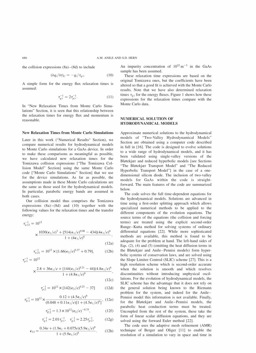
the collision expressions (8a)–(8d) to include

ð›qi=›tÞC ¼ 2qi=tq:i: ð10Þ

A simple form for the energy flux relaxation times is

assumed:

t21q:i ¼ 2t21

p:i : ð11Þ

In “New Relaxation Times from Monte Carlo Simu-

lations” Section, it is seen that this relationship between

the relaxation times for energy flux and momentum is

reasonable.

New Relaxation Times from Monte Carlo Simulations

Later in this work (“Numerical Results“ Section), we

compare numerical results for hydrodynamical models

to Monte Carlo simulations for a GaAs device. In order

to make these comparisons as meaningful as possible,

we have calculated new relaxation times for the

Tomizawa collision expressions [“The Tomizawa Col-

lision Model” Section] using the same Monte Carlo

code [“Monte Carlo Simulations” Section] that we use

for the device simulations. As far as possible, the

assumptions made in these Monte Carlo calculations are

the same as those used for the hydrodynamical models.

In particular, parabolic energy bands are assumed in

both cases.

Our collision model thus comprises the Tomizawa

expressions (8a)– (8d) and (10) together with the

following values for the relaxation times and the transfer

energy:

t21n:12 ¼ 1012

£1030ðe1=eÞ3 þ ½514ðe1=eÞ0:08 2 434�ð4e1=eÞ6

1 þ ð4e1=eÞ6;

ð12aÞ

t21n:21 ¼ 1012 £ ½1:66ðe2=eÞ0:37 þ 0:79�; ð12bÞ

t21p:1 ¼ 1012

£2:8 þ 36e1=e þ ½144ðe1=eÞ0:21 2 44�ð4:8e1=eÞ6

1 þ ð4:8e1=eÞ6;

ð12cÞ

t21p:2 ¼ 1012 £ ½142ðe2=eÞ0:25 2 37� ð12dÞ

t21E:1 ¼ 1012 £

0:12þ ð4:5e1=eÞ6

ð0:048 þ 0:11e1=eÞ½1 þ ð4:5e1=eÞ6�; ð12eÞ

t21E:2 ¼ 1:3£ 1012ðe2=eÞ20:75; ð12fÞ

t21q:1 ¼ 2:01t21

p:1 ; t21q:2 ¼ 2:25t21

p:2 ; ð12gÞ

e12 ¼0:34eþ ð1:9e1 þ 0:075eÞð5:9e1=eÞ6

1þ ð5:9e1=eÞ6: ð12hÞ

An impurity concentration of 1022 m23 in the GaAs

sample has been assumed.

These relaxation time expressions are based on the

original Tomizawa ones, but the coefficients have been

altered so that a good fit is achieved with the Monte Carlo

results. Note that we have also determined relaxation

times tq:i for the energy fluxes. Figure 1 shows how these

expressions for the relaxation times compare with the

Monte Carlo data.

NUMERICAL SOLUTION OF

HYDRODYNAMICAL MODELS

Approximate numerical solutions to the hydrodynamical

models of “Two-Valley Hydrodynamical Models”

Section are obtained using a computer code described

in full in [16]. The code is designed to evolve solutions

to a wide range of hydrodynamical models, and it has

been validated using single-valley versions of the

Bløtekjær and reduced hyperbolic models [see Sections

“The Bløtekjær Transport Model” and “The Reduced

Hyperbolic Transport Model”] in the case of a one-

dimensional silicon diode. The inclusion of two-valley

models for GaAs within the code is straight-

forward. The main features of the code are summarized

below.

The code solves the full time-dependent equations for

the hydrodynamical models. Solutions are advanced in

time using a first-order splitting approach which allows

specialized numerical methods to be applied to the

different components of the evolution equations. The

source terms of the equations (the collision and forcing

terms) are treated using the explicit second-order

Runge–Kutta method for solving systems of ordinary

differential equations [22]. While more sophisticated

methods are available, this method is found to be

adequate for the problem at hand. The left-hand sides of

Eqs. (2), (4) and (5) (omitting the heat diffusion terms in

the Bløtekjær and Anile–Pennisi models) form hyper-

bolic systems of conservation laws, and are solved using

the Slope Limiter Centred (SLIC) scheme [27]. This is a

high resolution scheme which is second-order accurate

when the solution is smooth and which resolves

discontinuities without introducing unphysical oscil-

lations. For the evolution of hydrodynamical models, the

SLIC scheme has the advantage that it does not rely on

the general solution being known to the Riemann

problem for the system, and indeed for the Anile–

Pennisi model this information is not available. Finally,

for the Bløtekjær and Anile–Pennisi models, the

parabolic heat conduction terms must be treated.

Uncoupled from the rest of the system, these take the

form of linear scalar diffusion equations, and they are

solved using the forward Euler method [22].

The code uses the adaptive mesh refinement (AMR)

technique of Berger and Oliger [11] to enable the

resolution of a simulation to vary in space and time in


response to the behaviour of the evolving solution. This

can greatly improve the speed with which numerical

results are obtained. For most of the GaAs device

simulations we describe here, a base resolution of

Dx ¼ L/200 was used (where L ¼ 2mm is the length of

the device). In regions surrounding jumps in the doping

profile nD, the resolution was increased to Dx ¼ L=800

via buffer regions of intermediate resolution

Dx ¼ L/400. A minimum resolution of Dx ¼ L=400

was also used in regions where the gradient or the

curvature of either of the velocity variables vi was

judged by the code to be high. These criteria for

dynamically varying the resolution have previously

been found to be effective in producing accurate results

for time-dependent simulations of a ballistic silicon

diode [16].

THE GAAS DIODE AND CIRCUIT

Our studies are based on a GaAs notched diode, as used by

Chen et al. [13]. This is coupled to an RLC tank circuit

which stimulates Gunn oscillatory effects. The same

configuration is used for both hydrodynamical and Monte

Carlo simulations.

The (one-dimensional) diode has length L ¼ 2mm and

is doped with donor atoms in a profile

nDðxÞ ¼

1023 for x , 0:125mm;

1022 for 0:125mm , x , 0:15mm;

0:5 £ 1022 for 0:15mm , x , 0:1875mm;ðdonors=m3Þ

1022 for 0:1875mm , x , 1:875mm;

1023 for 1:875mm , x:

8>>>>>>>>>><>>>>>>>>>>:

ð13Þ

In our studies, the transitions in the doping profile at

the device junctions are discontinuous (in contrast to

Ref. [13].

For both hydrodynamical and Monte Carlo simulations,

the following initial data at time t ¼ 0 is used:

n1 ¼ nDðxÞ; n2 ¼ 0; vi ¼ 0; Ti ¼ T0;

qi ¼ 0;ð14Þ

for i ¼ 1; 2: (In fact, for the hydrodynamical models, an

effective zero of 1013 m23 is used for the initial

number density n2 of electrons in the second valley.)

FIGURE 1 Relaxation rates from Monte Carlo simulations. The grey dots in the figure show results from two-valley Monte Carlo simulations of ahomogeneous GaAs sample for the relaxation times for particle transfers tn:ij; momenta tp:i; energies tE:i and energy fluxes tq:i; together with the averagetransfer energy between valleys e12. The results are presented as functions of the electron energy e i for the appropriate valley. The analytic expressions(12a)–(12h) which have been fitted to the Monte Carlo data are shown in the figure as solid lines. For comparison, the Tomizawa relaxation expressions(9a)–(9g) are shown as dashed lines.


For the Monte Carlo simulations, this initial state is

implemented by starting all particles off in the first valley

with velocities randomly picked to give a Maxwellian

distribution.

The following boundary conditions at x ¼ 0 and x ¼ L

are used for the hydrodynamical simulations:

n1 ¼ nD; n2 ¼ 0; vi ¼ 0; Ti ¼ T0; qi ¼ 0: ð15Þ

Implementation of equivalent boundary conditions in the

Monte Carlo simulations is not entirely straightforward.

The approach we use is to extend the Monte Carlo

domain to include short “buffer” regions beyond the

specified edges of the device. During the course of a

simulation the number density of electrons in these

buffer regions is made to be constant, equal to the

doping density nD at the contacts, by removing at

random excess electrons, or creating replacement

electrons in the first valley with velocities fitting a

Maxwellian distribution consistent with Eq. (15).

Simulation results are not found to be overly sensitive

to the conditions at the boundaries.

Boundary conditions for Poisson’s equation (1) are

imposed by specifying the electric potential at the device

contacts:

fð0Þ ¼ 0; fðLÞ ¼ V: ð16Þ

Here the potential difference V is either a prescribed

function of the simulation time (typically a constant value

of 2 V), or it is determined by coupling the device to a

system of ODEs modelling a simple circuit.

For simulating Gunn oscillations we use the following

circuit model given by Chen et al. [13]. The voltage V

across the device and the current I through the battery

satisfy differential equations

dV

dt¼

1

CI 2 Id 2

V

R

;

dI

dt¼

1

LVB 2 Vð Þ; ð17Þ

where the particle current in the device is calculated as

Id ¼eA

L

ðL

0

ðn1v1 þ n2v2Þdx; ð18Þ

or an equivalent summation over particles for Monte

Carlo simulations. Simple finite difference versions of

Eqs. (17) and (18) allow the diode voltage to be

updated at each simulation time step. The values used

for the capacitance, resistance and inductance of the

circuit are

C ¼ 1A=L þ 0:82 £ 10212; R ¼ 25;

L ¼ 3:5 £ 10212;

where 1 is the dielectric constant of GaAs, L is the

diode length, and its cross-sectional area is

A ¼ 1:0 £ 1029 m2:

The bias voltage of the circuit is

VB ¼ 2 V;

and the oscillator equations (17) are given the initial

state

Vðt0Þ ¼ VB Iðt0Þ ¼ 0: ð19Þ

when the circuit is engaged at time t0.

NUMERICAL RESULTS

We present numerical results for the two-valley hydro-

dynamical models of “Two-Valley Hydrodynamical

Models” Section. Comparisons are made with the results

of Chen et al. [13] [see “Comparison with Existing

Results” Section], and between hydrodynamical and

Monte Carlo simulations for a homogeneous sample [see

“Simulations of Homogeneous Samples” Section], and for

a diode both at steady state [see “Device Behaviour at

Steady State” Section] and when coupled to an oscillator

circuit [see “Gunn Oscillations” Section].

Comparison With Existing Results

To validate our numerical approach for two-valley

hydrodynamical models [“Numerical Solution of Hydro-

dynamical Models” Section], we have reproduced the

GaAs diode simulations of CJSW [3].

The semiconductor model used combines the Bløtekjær

transport equations of “The Bløtekjær Transport Model”

Section with the CJSW collision expressions of “The

CJSW Collision Model” Section. For the electron

effective masses, CJSW use values m*1 ¼ 0:065 me and

m*2 ¼ 0:222 me which are different from the values we use

for the other simulations described here. The GaAs diode

and oscillator circuit are as described in “The GaAs Diode

and Circuit” Section with the difference that for the CJSW

simulations the doping profile is smooth across the device

junctions.

Numerical results are presented by CJSW for the steady

state of the device under a fixed voltage and for its

oscillatory behaviour when coupled to a circuit. We obtain

results which are in good agreement in all cases. What

differences there are may be plausibly attributed to the

different resolutions and numerical methods used. (The

CJSW simulations use a third-order ENO scheme with

Runge–Kutta time stepping.)

We note that the differences in the effective masses and

the doping profile mentioned above are observed to have

significant effects on simulation results.

Simulations of Homogeneous Samples

The first of our comparisons between hydrodynamical

models and Monte Carlo results considers the case of

homogeneous GaAs samples when fixed electric fields


are applied. For the hydrodynamical models, the

evolution equations reduce to systems of ODEs which

are easily integrated using the Runge–Kutta method to

obtain steady solutions. For the Monte Carlo simu-

lations, a simplified version of the code described in

“Monte Carlo Simulations” Section is used in which a

single particle is tracked and its behaviour time-

averaged to determine macroscopic properties at steady

state.

Figure 2 shows steady state results over a range of

electric field strengths, with Monte Carlo results being

contrasted against hydrodynamical solutions. The

reduced hyperbolic transport model (5) combined with

the Tomizawa collision terms (8a)–(8d) is solved for

two different sets of relaxation times: those of

Tomizawa (9a)–(9g) and the values (12a)–(12h) derived

from Monte Carlo calculations. When the same collision

expressions are used, results for the Bløtekjær and

Anile–Pennisi transport models are identical to those of

the reduced hyperbolic model in the homogeneous case.

(The latter are shown in Fig. 2 because they include

values for the energy fluxes qi). When the CJSW

collision terms [“The CJSW Collision Model” Section]

are used with the Bløtekjær transport model the results

show little agreement with the Monte Carlo simulations,

which is not surprising given the simplistic nature of the

relaxation times.

It may be observed from Fig. 2 that the new relaxation

times (12a)–(12h) give a better agreement overall with the

Monte Carlo results than the Tomizawa expressions do.

This is to be expected, of course, since these relaxation

times are derived using the same Monte Carlo code and

the same physical assumptions. However, in neither case is

the agreement between hydrodynamical and Monte Carlo

results perfect, and this highlights the limitations of the

relaxation time approach for modelling collision pro-

cesses: more detailed models may be needed to accurately

capture semiconductor behaviour, even in the homo-

geneous case.

Device Behaviour at Steady State

The GaAs diode described in “The GaAs Diode and

Circuit” Section is evolved to steady state under a fixed

applied voltage to provide another comparison between

semiconductor models.

The initial state of the device is given by Eqs. (13) and

(14), and the boundary conditions by Eq. (15). A voltage

FIGURE 2 Steady state results for homogeneous GaAs. A comparison is made between two hydrodynamical models and Monte Carlo simulations.Solutions are shown to the reduced hyperbolic hydrodynamical equations [“The Reduced Hyperbolic Transport Model” Section] with collision termsbased on the Tomizawa relaxation times [“The Tomizawa Collision Model” Section, the dashed lines] and new relaxation times derived from MonteCarlo calculations [“New Relaxation Times from Monte Carlo Simulations” Section, the solid lines]. The grey dots show comparable results from directMonte Carlo simulations.


of V ¼ 2 V is used in Eq. (16). To avoid initiating

too much complicated transient behaviour in the device,

the voltage is slowly raised to this value, starting from

zero, over a time of 15 ps. Simulations are run to a final

time of t ¼ 75 ps; at which the hydrodynamical solutions

are judged to change by only negligible amounts on each

time step.

Figure 3 shows results from two hydrodynamical

models together with comparable Monte Carlo simu-

lations. The Bløtekjær model is used with the

Tomizawa collision expressions [see Sections “The

Bløtekjær Transport Model” and “The Tomizawa

Collision Model”], and the reduced hyperbolic model

is used with the relaxation times derived from Monte

Carlo calculations [see Sections “The Reduced Hyper-

bolic Transport Model“ and “New Relaxation Times

from Monte Carlo Simulations”]. It has previously been

observed [16] for a silicon diode that the steady state

solutions for the Bløtekjær and the reduced hyperbolic

transport models (which differ significantly only in

their treatment of heat conduction) are very similar if

both use the same collision terms. This has been found

to be the case also for the GaAs diode (and also when

the Anile–Pennisi transport model is considered), and

consequently results for other combinations of transport

and collision models are not presented in Fig. 3. For

the CJSW collision model [“The CJSW Collision

Model” Section] the numerical results differ substan-

tially from the Monte Carlo calculations, as would be

expected.

It may be seen from Fig. 3 that the hydrodynamical

models give solutions which are broadly in agreement

with the Monte Carlo results. However, the agreement is

not perfect, and, perhaps surprisingly, the results obtained

using the Tomizawa relaxation times may be judged to be

closer to the Monte Carlo results than the ones obtained

using relaxation times derived from the same Monte Carlo

code. This suggests that the “effective” relaxation times

for a device may be different from the relaxation times for

a homogeneous sample.

FIGURE 3 Steady state results for the GaAs diode. A comparison is made between two hydrodynamical models and Monte Carlo simulations. Thedashed lines show results for the Bløtekjær hydrodynamical model [“The Bløtekjær Transport Model” Section] with the Tomizawa collision terms [“TheTomizawa Collision Model” Section]. The black lines show results for the reduced hyperbolic model [“The Reduced Hyperbolic Transport Model”Section] with relaxation times based on Monte Carlo calculations [“New Relaxation Times from Monte Carlo Simulations” Section]. The grey linesshow results from direct Monte Carlo simulations.


Gunn Oscillations

For our final comparison between models, we consider the

time-dependent behaviour of a GaAs diode subject to

Gunn oscillations.

“The GaAs Diode and Circuit” Section describes the

circuit used to determine the voltage across the diode.

In our simulations, the circuit is engaged at the time

when the GaAs diode is judged to have reached the

steady state discussed in “Numerical Results” Section.

(The applied voltage V ¼ 2 V for the steady state is the

initial voltage used in the circuit model.)

Figure 4 shows the voltage V(t ) across the device for

Gunn oscillations in seven hydrodynamical models and

also for a Monte Carlo simulation. It is apparent from

the figure that significantly different results are produced

by the different models: the oscillations can initially

grow or decay, and may reach a steady amplitude or

eventually vanish. The hydrodynamical results closest to

the Monte Carlo ones are for the reduced hyperbolic

transport model when the Tomizawa collision terms are

used [see Sections “The Reduced Hyperbolic Transport

Model” and “The Tomizawa Collision Model”],

although the decay rates of the oscillations in the two

cases are clearly different. (The small oscillations seen in

the Monte Carlo results at late times are believed to be

spurious: as the number of particles used in simulations

increases, the amplitude of these oscillations decreases,

and it is likely that they would not be present in a

“converged” solution produced using sufficiently many

particles.)

It may be noted from Fig. 4 that there are significant

differences between results for the three different transport

models we use (the Bløtekjær, Anile–Pennisi and reduced

hyperbolic models). This is in contrast to the steady state

results obtained for the device [“Device Behaviour at

Steady State” Section] and reinforces the tentative

FIGURE 4 Gunn oscillations in a GaAs diode for eight different simulations. The device voltage V is shown for the circuit described in “The GaAsDiode and Circuit” Section. Results are presented from seven hydrodynamical models. The Bløtekjær transport model [“The Bløtekjær TransportModel” Section] is tested with three different collision models (Sections “The CJSW Collision Model”, “The Tomizawa Collision Model” and “NewRelaxation Times from Monte Carlo Simulations”], while the Anile–Pennisi [“The Anile–Pennisi Transport Model” Section] and reduced hyperbolictransport models [“The Reduced Hyperbolic Transport Model” Section] are both tested with two collision models [Sections “The Tomizawa CollisionModel” and “New Relaxation Times from Monte Carlo Simulations”]. (For the CJSW collision model, the threshold energy is taken asa ¼ 1:44 £ 10220 J:) Results from a Monte Carlo simulation are also shown.


conclusion of Ref. [16] (for a silicon diode) that the form

of heat conduction used in a hydrodynamical model has

more of an effect on time-dependent behaviour than on

steady state behaviour.

CONCLUSIONS

We have compared numerical results for a variety of

hydrodynamical models against Monte Carlo simulations

for a GaAs diode both at steady state and when producing

Gunn oscillations. The usefulness of hydrodynamical

models in semiconductor device design is apparent:

using modern numerical methods, accurate solutions for

the models have been obtained in minutes, compared to

Monte Carlo running times of possibly several days.

However, while the hydrodynamical results are reasonably

close to the Monte Carlo ones for the diode at steady state,

only one of the hydrodynamical models tested produced

Gunn oscillations similar to those of the Monte Carlo

code.

The results of this study suggest (very tentatively) that

the “reduced hyperbolic” transport model coupled to the

Tomizawa collision model gives the most realistic results

for GaAs devices. It is perhaps surprising that the

Tomizawa relaxation expressions produce better results

than alternative expressions derived specifically to be

consistent with the Monte Carlo code in the homogeneous

case. However, as has already been remarked, it could

be that the “effective” relaxation times for the device are

different from the homogeneous ones due to the influence

of higher moments caused by, for example, jumps in

the density. The Tomizawa expressions might, by chance,

provide a better fit to these inhomogeneous relaxation

rates. This calls for further work to be done in deriving

semiconductor models within the moments framework,

with higher moments being systematically included to

capture complicated time-dependent behaviour such as

Gunn oscillations.

Acknowledgements

This research was supported by the TMR network

“Asymptotic Methods in Kinetic Theory,” contract

number ERB FMRX CT97 0157, and CNR contracts

97.00342.CT11 and 97.04713.CT01.

References

[1] Alekseev, E. and Pavlidis, D. (2000) “Large-signal microwaveperformance of GaN-based NDR diode oscillators”, Solid-StateElectron. 44, 941–947.

[2] Anile, A.M. and Muscato, O. (1995) “Improved hydrodynamicalmodel for carrier transport in semiconductors”, Phys. Rev. B 51,16728–16740.

[3] Anile, A.M., Nikiforakis, N. and Pidatella, R.M. (2000) “Momentequations for carrier transport in semiconductors”, In: Fiedler, B.,Groger, K. and Sprekels, J., eds, International Conference onDifferential Equations, Berlin 1999 (World Scientific).

[4] Anile, A.M., Nikiforakis, N. and Pidatella, R.M. (2000)“Assessment of a high resolution centred scheme for the solutionof hydrodynamical semiconductor equations”, SIAM J. Sci.Comput. 22(5), 1533–1548.

[5] Anile, A.M. and Pennisi, S. (1992) “Thermodynamic derivation ofthe hydrodynamical model for charge transport in semiconductors”,Phys. Rev. B 46, 13186–13193.

[6] Anile, A.M., Romano, V. and Russo, G. (1998) “Hyperbolichydrodynamical model of carrier transport in semiconductors”,VLSI Design 8, 521–525.

[7] Anile, A.M., Romano, V. and Russo, G. (2000) “Extendedhydrodynamical model of carrier transport in semiconductors”,SIAM J. Appl. Math. 61, 74–101.

[8] Anile, A.M. and Romano, V. (1999) “Nonparabolic band transportin semiconductors: closure of the moment equations”, Cont. Mech.Thermodyn. 11, 307–325.

[9] Anile, A.M. and Trovato, M. (1997) “Nonlinear closures forhydrodynamical semiconductor transport models”, Phys. Lett. A230, 387–395.

[10] Ben Abdallah, N., Degond, P. and Genieys, S. (1996) “An energy-transport model for semiconductors derived from the Boltzmannequation”, J. Stat. Phys. 84, 205–231.

[11] Berger, M.J. and Oliger, J. (1984) “Adaptive mesh refinement forhyperbolic partial differential equations”, J. Comput. Phys. 53,484–512.

[12] Bløtekjær, K. (1970) “Transport equations for electrons intwo-valley semiconductors”, IEEE Trans. Electron Devices 17,38–47.

[13] Chen, G.-Q., Jerome, J.W., Shu, C.W. and Wang, D. (1998)“Two carrier semiconductor device models with geometricstructure and symmetry properties”, In: Jerome, J., ed,Modelling and Computation for Applications in Mathematics,Science, and Engineering (Oxford University Press, Oxford), pp103–140.

[14] Curow, M. and Hintz, A. (1987) “Numerical simulation ofnonstationary electron transport in Gunn devices in a harmonicmode oscillator circuit”, IEEE Trans. Electron Devices 34,1983–1994.

[15] Gruzinski, V., Starikov, E., Shiktorov, P., Reggiani, L. and Varani, L.(1994) “Linear and nonlinear analysis of microwave powergenerator in sub-micrometer n þ–n–n þ InP diodes”, J. Appl.Phys. 76, 5260–5271.

[16] Hern, S.D., Anile, A.M., Nikiforakis, N., “A mesh refinementapproach for hydrodynamical semiconductor simulations”, J. Comp.Phys., In press.

[17] Jacoboni, C. and Lugli, P. (1989) The Monte Carlo Method forSemiconductor Device Simulation (Springer, New York).

[18] Jou, D., Casas-Vazquez, J. and Lebon, G. (1993) ExtendedIrreversible Thermodynamics (Springer, Berlin).

[19] Levermore, C.D. (1998) “Moment closure hierarchies for theBoltzmann–Poisson equation”, VLSI Design 6, 97–101.

[20] Markowich, A., Ringhofer, C.A. and Schmeiser, C. (1990)Semiconductor Equations (Springer, Wien).

[21] Muller, I. and Ruggeri, T. (1998) Rational Extended Thermodyn-amics (Springer, New York).

[22] Press, W., Teukolsky, S.A., Vetterling, W.T. and Flannery, B.P.(1992) Numerical Recipes, 2nd Ed. (Cambridge University Press,Cambridge).

[23] Romano, V. (2000) “Nonparabolic band transport in semiconduc-tors: closure of the production terms”, Cont. Mech. Thermodyn. 12,31–51.

[24] Romano, V. and Russo, G. (2000) “Numerical solution forhydrodynamical models of semiconductors”, Math. ModelsMethods Appl. Sci. 10, 1099–1120.

[25] Tomizawa, K. (1993) Numerical Simulation of SubmicronSemiconductor Devices (Artech House, Boston-London).

[26] Tomizawa, K. and Pavlidis, D. (1990) “Transport equation approachfor heterojunction bipolar transistors”, IEEE Trans. ElectronDevices 37, 519–529.

[27] Toro, E.F. (1997) Riemann Solvers and Numerical Methods forFluid Dynamics (Springer, New York).

[28] Zybura, M.F., Jones, S.H., Tait, C.B. and Jonesl, J.R. (1994) “100–300 GHz Gunn oscillator simulation through harmonic balancecircuit analysis linked to a hydrodynamic device simulator”, IEEEMicrowave Guided Wave Lett. 4, 282–284.


Angelo Marcello Anile Graduated in Mathematics from

the Scuola Normale Superiore of Pisa (Italy). Doctor

Degree from Oxford University. Presently Professor of

Applied Mathematics in the University of Catania.

Member of the Editorial Board of CONTINUUM

MECHANICS and THERMODYNAMICS. The scientific

interests have developed along three phases: (i) First

phase: mathematical models for astrophysics, mainly

relativistic fluids and plasmas; (ii) Second phase: non-

linear wave propagation with applications to plasmas; (iii)

Third phase (present): mathematical models for carrier

transport in semiconductor devices. The author is the

leader of a research group in applied mathematics which

has active collaboration with industry, in particular with

ST-Microelectronics for mathematical modeling of

semiconductor devices (particularly transport in submi-

cron devices and optimization). Author of over 90

publications in refereed journals and 2 books.

Simon Hern, Graduated from the University of Notting-

ham, UK, in 1994. He received a Ph.D. from the

University of Cambridge, UK, for research into the

numerical solution of problems in relativistic gravity, and

until 2001 did post-doctoral research on models of

electron transport in semiconductors at the university of

Catania, Italy.


International Journal of

AerospaceEngineeringHindawi Publishing Corporationhttp://www.hindawi.com Volume 2010

RoboticsJournal of

Hindawi Publishing Corporationhttp://www.hindawi.com Volume 2014


Active and Passive Electronic Components

Control Scienceand Engineering

Journal of



RotatingMachinery


Hindawi Publishing Corporation http://www.hindawi.com

Journal ofEngineeringVolume 2014

Submit your manuscripts athttp://www.hindawi.com

VLSI Design



Shock and Vibration


Civil EngineeringAdvances in

Acoustics and VibrationAdvances in



Electrical and Computer Engineering

Journal of

Advances inOptoElectronics

Hindawi Publishing Corporation http://www.hindawi.com

Volume 2014

The Scientific World JournalHindawi Publishing Corporation http://www.hindawi.com Volume 2014

SensorsJournal of


Modelling & Simulation in EngineeringHindawi Publishing Corporation http://www.hindawi.com Volume 2014


Chemical EngineeringInternational Journal of Antennas and

Propagation




Navigation and Observation



DistributedSensor Networks


two-valley hydrodynamical models for electron transport in...

Documents