two-stage high efficiency air conditioners: …€¦ · 1 two-stage high efficiency air...
TRANSCRIPT
D507
Creators of CheckMe!®
Prepared by: Proctor Engineering Group, Ltd.
San Rafael, CA 94901 (415) 451-2480
Two-Stage High Efficiency Air Conditioners: Laboratory Ratings vs. Residential Installation
Performance
Presented at: ACEE 2006
Contributors: John Proctor, P.E.
Gabriel Cohn

1
Two-Stage High Efficiency Air Conditioners:
Laboratory Ratings vs. Residential Installation Performance
John Proctor and Gabriel Cohn , Proctor Engineering Group, Ltd.
ABSTRACT
The increased installation of high Seasonal Energy Efficiency Ratio (SEER) air conditioners
along with utility program rebates for these units prompted a study of the measured performance of
these systems. This project assessed the performance of these systems in the climate zones found in the
mid-Atlantic region of the U.S. Similar studies in hot dry climates have indicated that laboratory SEER
ratings may not properly predict the actual impact of these systems.
This project monitored four high SEER air conditioners with dual-stage compressors, TXV
metering devices, and high efficiency air handlers with ECM fan motors. One system with a single-stage
compressor was also monitored. Data included capacity, power consumption, EER, indoor/outdoor
temperature and relative humidity. The data were analyzed to assess the relationship between laboratory
testing and real world performance.
This study found causes for concern including: actual seasonal energy efficiency ratios between
59% and 84% of the rated SEERs, constant fan operation substantially degrading seasonal efficiencies
and reducing dehumidification, latent loads that exceed Manual J estimates, and sensible loads
substantially lower than Manual J estimates. In addition there may be an energy and peak load penalty if
dual-stage air conditioners are downsized to near the buildings’ actual loads.
The study illustrates the intricacy of the whole building system. The air conditioners in the two
leakiest building shells were unable to adequately control the indoor humidity.
Introduction
Utilities and contractors across the United States have successfully promoted the installation of
high SEER central air conditioning systems. High SEER systems are often equipped with dual-stage
compressors and variable speed blowers. This study addressed the impact of these systems on the
electric grid in DOE Climate Zones 4 and 5. The test houses were located in New Jersey and New York
at the Northern edge of Climate Zone 4 and the Southern edge of Climate Zone 5. Both climate zones
are considered “moist”, where outdoor air often contributes to the latent load on the air conditioner.
A continuing question in the energy-efficiency community is how closely SEER ratings
represent the actual seasonal efficiency of air conditioners in various climates. Given the increasing
frequency of these installations and emphasis of utility programs on installing higher efficiency SEER
equipment, it is important to quantify the impact of these high efficiency systems.
The purpose of this study was to compare the operating characteristics (peak demand, EER, and
kWh) of high efficiency residential central air conditioning systems to projections from ratings including
SEER and EER.
D507

2
One of the objectives of this study was to compare dual-stage units against a high efficiency
single speed unit. This study monitored four recently installed dual-stage air conditioners and one high
efficiency single speed AC system.
Monitoring System
Each air conditioner was monitored by a data acquisition system (DAS). The DAS has the
flexibility to perform many data acquisition functions and is capable of being downloaded or
reprogrammed via modem. The temperature probes were bare wire 36 gauge type T thermocouples,
RTDs, or thermistors. Condensate flow from the indoor coil was measured with the use of a tipping
bucket gauge attached to the termination of the condensate drain. Data points are summarized in Table
1.
Table 1. Monitored Points Measurement Sensor Type Sensor Location
Supply Air Dry Bulb Temperature 4 Point RTD Grid After Coil In Supply Plenum
Supply Air Dry Bulb Temperature Thermister After Coil In Supply Plenum
Supply Air Dry Bulb Temperature Thermocouple After Coil In Supply Plenum
Supply Air Dry Bulb Temperature Thermocouple Far Supply Register
Supply Air Dry Bulb Temperature Thermocouple Near Supply Register
Supply Air Relative Humidity Humidity Transmitter With Supply Air Thermister
Return Air Dry Bulb Temperature Thermister Return Plenum Before Furnace
Return Air Dry Bulb Temperature Thermocouple Return Plenum Before Furnace
Return Air Dry Bulb Temperature Thermocouple Return Grill
Return Air Relative Humidity Humidity Transmitter With Return Air Thermister
Buffer Space Dry Bulb Temperature Thermocouple Buffer Space
Outside Air Temperature Thermister (Shielded) Outside Near Condensing Unit
Outside Air Relative Humidity Humidity Transmitter With Outside Air Thermister
Indoor Air Temp Thermister Near Thermostat
Compressor Discharge Temperature RTD Surface Mounted To Compressor Gas
Discharge Line (Insulated)
Refrigerant Liquid Line Temperature RTD Surface Mounted To Liquid Line After
Condenser Coil (Insulated)
Condenser Saturation Temperature 2 Thermocouples Surface Mounted to Condenser
Refrigerant Circuit
Evaporator Saturation Temperature 2 Thermocouples Surface Mounted to Evaporator
Refrigerant Circuit
Vapor Suction Line Temperature RTD Surface Mounted To Suction Line
Before Compressor (Insulated)
Evaporator Condensate Flow Tipping Bucket Evaporator Condensate Line
Compressor Current Current Transducer Compressor Power lines
Furnace Blower Current Current Transducer Blower Power Lines
Furnace Gas Valve Current Current Transducer Gas Valve Control Lines
Condensing Unit Power Watt Transducer Electrical Supply To Unit
Furnace Blower Power Watt Transducer Electrical Supply To Furnace Unit
D507

3
Site Descriptions
The characteristics of the homes and air conditioners in the project convenience sample are listed
in Table 2.
Table 2. Site Characteristics
House Specifications
Site P1 Site S Site T Site N Site W
House Size (square feet) 1620 2375 1900 3500 2300
Year Built 2002 2000 1940s 1960s 1970s
Manual J7 Cooling Load (Btuh) at 90/75/63
no window coverings 22118 36342 27513 56462 29549
Manual J7 Cooling Load (Btuh) at 90/75/63 with drapes 18180 29471 22851 44106 23864
House Tightness: Air Changes per Hour (ACH50) 3.9 2.8 5.5 7.4 12.7
Air to Air Heat Exchanger Flow (% of airflow) 17% 12% none none none
% of Time Indoor RH >60% 2% 13% 0% 40% 35%
Air Conditioner Specifications
Rated SEER 14.25 14 15 14 14
High Speed Rated EER at 95/80/67 10.3 10.7 9.4 10.8 11.5
Low Speed Rated EER at 95/80/67 None 12.2 11.7 12.4 12.6
High Speed Rated Capacity at 95/80/67 (Btuh) 34900 46080 34300 48230 48230
Low Speed Rated Capacity at 95/80/67 (Btuh) None 25260 24700 27180 27180
Number of Compressor Speeds 1 2 2 2 2
Metering Device Fixed TXV TXV TXV TXV
Fan Motor Hp 1/2 Hp 1 Hp 1 Hp 1 Hp 1 Hp
Fan Motor Type ECM ECM ECM ECM ECM
Fan Mode (TD = Time Delay IO = Instant Off) TD Const. TD IO Const.
1. ARI ratings are not available for the Site P system combination (using a third party evaporator coil). The estimated rated
SEER, EER, power, and capacities are for a manufacturer’s combination with the same nominal capacity.
House Characteristics
All the sites were 2 story homes with furnaces and ducts in the basement. Site P is a new
modular home and Site S is a new Energy Star home.
The homes were tested for air leakage using a single point (50 pascals) blower door test. There
was a large variation in the measured air leakage (2.8 ACH50 to 12.7 ACH50). Sites N and W were the
leakiest homes and the dual-stage/variable airflow air conditioners were unable to adequately control the
inside relative humidity.
The cooling loads were calculated using Manual J7 at an inside/outside temperature difference of
15 °F, with an infiltration rate estimated from the blower door test, with latent and sensible loads
calculated independently, with the swing factor set to 1, and with no window coverings. Site N has a
Manual J 7 estimated load that exceeds the nominal tonnage of the installed air conditioner – an unusual
situation.
Aggressive Manual J7 load estimates were also calculated based on interior drapes on all the
windows.
D507

4
Air Conditioner Specifications
The air conditioners represented a narrow band of efficiencies from 14 to 15. The units were
three-ton and four-ton units. There were three different types of furnace fan operation observed in these
units: Constant on – this produces the minimum latent capacity since moisture on the coil at the end of
the compressor cycle is evaporated back into the house air; Time delay – this is the most common fan
control which is designed to maximize the SEER of the unit; and Instant off – the fan control which
should produce the most latent cooling (moisture removal). Two homes used a constant fan. One home
used the constant fan to circulate air around musical instruments, pianos, cellos, etc. The other home
began using a constant fan part-way through the summer for an unknown reason.
D507

5
Results
Cooling Season results are tabulated by 5ºF temperature bins and compared to the
manufacturer’s ratings. Tables 3 and 4 display the results for the 80ºF to 85ºF temperature bin. Complete
results are available in Proctor, Cohn & Conant 2006.
End of Cycle Performance
The End of Cycle (EOC) data are obtained by taking the sensor measurements from the last full
minute of compressor operation for each cycle. This point is used to compare performance to the
manufacturers’ steady state ratings because it is the point in the cycle closest to steady state operation.
The results are displayed in Tables 3 and 4.
Low Speed. Sites P and T do not have low speed data because the former is a single speed machine and
the latter dual speed machine that ran only on high speed. At low speed the other three units achieved
89% or better of the rated capacity and their input power exceeded the rated values by 10% or more. The
unit at Site N approached the rated capacity in this and other temperature bins.
Table 3. Low Speed Performance
Site P Site S Site T Site N Site W
Average Outside Temperature (deg F) NA 82.3 NA 82.3 82.1
Average Return Drybulb Temperature (deg F) NA 70.2 NA 71.1 73.7
Average Return Wetbulb Temperature (deg F) NA 63.8 NA 61.9 64.9
Average Cycle Length (min) NA 22.8 NA 62.1 64.7
Number of Cycles NA 414 NA 26 184
Capacity
End of Cycle Net Capacity (Btuh) NA 21529 NA 29230 24972
Mfr. Steady State (SS) Net Capacity (Btuh) NA 24333 NA 26855 26754
% of Mfr. Steady State Net Capacity NA 88% NA 109% 93%
End of Cycle Net Sensible Capacity (Btuh) NA 13483 NA 17225 17131
Mfr. SS Net Sensible Capacity (Btuh) NA 15080 NA 18415 18837
% of Mfr. SS Net Sensible Capacity (Btuh) NA 89% NA 94% 91%
Input Power
Total End of Cycle Input Power (W) NA 2011 NA 1943 2037
Mfr. Steady State Input Power (W) NA 1792 NA 1692 1860
% of Mfr. Steady State Input Power NA 112% NA 115% 110%
EER
End of Cycle EER NA 10.72 NA 15.09 12.27
Mfr. Steady State EER NA 13.59 NA 15.88 14.39
% of Mfr. Steady State EER NA 79% NA 95% 85%
High Speed. Site P, the single speed machine has performance inconsistent with other single speed ACs
field monitored by the authors (Proctor 1998, 5). Field monitored efficiencies for single speed air
D507
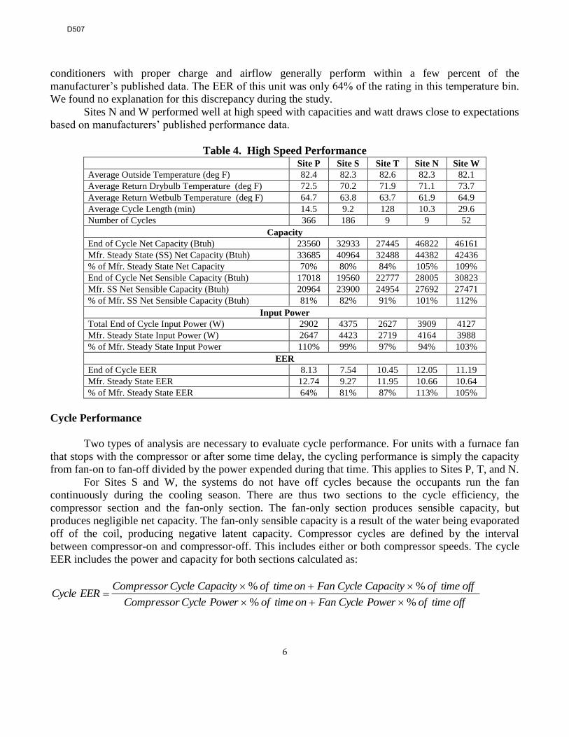
6
conditioners with proper charge and airflow generally perform within a few percent of the
manufacturer’s published data. The EER of this unit was only 64% of the rating in this temperature bin.
We found no explanation for this discrepancy during the study.
Sites N and W performed well at high speed with capacities and watt draws close to expectations
based on manufacturers’ published performance data.
Table 4. High Speed Performance Site P Site S Site T Site N Site W
Average Outside Temperature (deg F) 82.4 82.3 82.6 82.3 82.1
Average Return Drybulb Temperature (deg F) 72.5 70.2 71.9 71.1 73.7
Average Return Wetbulb Temperature (deg F) 64.7 63.8 63.7 61.9 64.9
Average Cycle Length (min) 14.5 9.2 128 10.3 29.6
Number of Cycles 366 186 9 9 52
Capacity
End of Cycle Net Capacity (Btuh) 23560 32933 27445 46822 46161
Mfr. Steady State (SS) Net Capacity (Btuh) 33685 40964 32488 44382 42436
% of Mfr. Steady State Net Capacity 70% 80% 84% 105% 109%
End of Cycle Net Sensible Capacity (Btuh) 17018 19560 22777 28005 30823
Mfr. SS Net Sensible Capacity (Btuh) 20964 23900 24954 27692 27471
% of Mfr. SS Net Sensible Capacity (Btuh) 81% 82% 91% 101% 112%
Input Power
Total End of Cycle Input Power (W) 2902 4375 2627 3909 4127
Mfr. Steady State Input Power (W) 2647 4423 2719 4164 3988
% of Mfr. Steady State Input Power 110% 99% 97% 94% 103%
EER
End of Cycle EER 8.13 7.54 10.45 12.05 11.19
Mfr. Steady State EER 12.74 9.27 11.95 10.66 10.64
% of Mfr. Steady State EER 64% 81% 87% 113% 105%
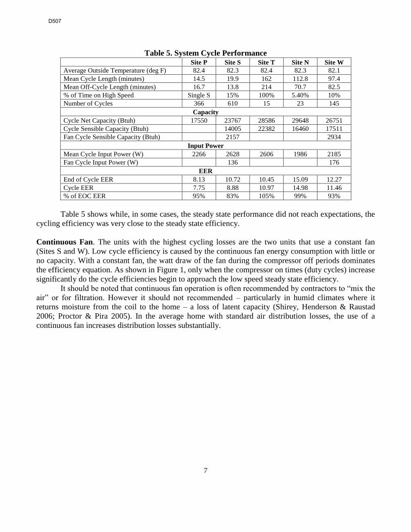
Cycle Performance
Two types of analysis are necessary to evaluate cycle performance. For units with a furnace fan
that stops with the compressor or after some time delay, the cycling performance is simply the capacity
from fan-on to fan-off divided by the power expended during that time. This applies to Sites P, T, and N.
For Sites S and W, the systems do not have off cycles because the occupants run the fan
continuously during the cooling season. There are thus two sections to the cycle efficiency, the
compressor section and the fan-only section. The fan-only section produces sensible capacity, but
produces negligible net capacity. The fan-only sensible capacity is a result of the water being evaporated
off of the coil, producing negative latent capacity. Compressor cycles are defined by the interval
between compressor-on and compressor-off. This includes either or both compressor speeds. The cycle
EER includes the power and capacity for both sections calculated as:
offtimeofPowerCycleFanontimeofPowerCycleCompressor
offtimeofCapacityCycleFanontimeofCapacityCycleCompressorEERCycle
%%
%%
D507
7
Table 5. System Cycle Performance Site P Site S Site T Site N Site W
Average Outside Temperature (deg F) 82.4 82.3 82.4 82.3 82.1
Mean Cycle Length (minutes) 14.5 19.9 162 112.8 97.4
Mean Off-Cycle Length (minutes) 16.7 13.8 214 70.7 82.5
% of Time on High Speed Single S 15% 100% 5.40% 10%
Number of Cycles 366 610 15 23 145
Capacity
Cycle Net Capacity (Btuh) 17550 23767 28586 29648 26751
Cycle Sensible Capacity (Btuh) 14005 22382 16460 17511
Fan Cycle Sensible Capacity (Btuh) 2157 2934
Input Power
Mean Cycle Input Power (W) 2266 2628 2606 1986 2185
Fan Cycle Input Power (W) 136 176
EER
End of Cycle EER 8.13 10.72 10.45 15.09 12.27
Cycle EER 7.75 8.88 10.97 14.98 11.46
% of EOC EER 95% 83% 105% 99% 93%
Table 5 shows while, in some cases, the steady state performance did not reach expectations, the
cycling efficiency was very close to the steady state efficiency.
Continuous Fan. The units with the highest cycling losses are the two units that use a constant fan
(Sites S and W). Low cycle efficiency is caused by the continuous fan energy consumption with little or
no capacity. With a constant fan, the watt draw of the fan during the compressor off periods dominates
the efficiency equation. As shown in Figure 1, only when the compressor on times (duty cycles) increase
significantly do the cycle efficiencies begin to approach the low speed steady state efficiency.
It should be noted that continuous fan operation is often recommended by contractors to “mix the
air” or for filtration. However it should not recommended – particularly in humid climates where it
returns moisture from the coil to the home – a loss of latent capacity (Shirey, Henderson & Raustad
2006; Proctor & Pira 2005). In the average home with standard air distribution losses, the use of a
continuous fan increases distribution losses substantially.
D507

8
Figure 1. Cycle EER Degradation from Continuous Fan (Dual-Stage Machine)
2
4
6
8
10
12
14
16
18
65 75 85 95
Outside Temperature (F)
EE
R
0%
20%
40%
60%
80%
100%
Du
ty C
yc
le
End of Cycle EER Cycle EERPercent On Time
Dual-Stage Units. The two dual-stage units with fan-off at or near compressor off show little or no
cycling degradation. The lack of degradation can be interpreted to indicate that there is little if any
savings available for downsizing these dual-stage units. This is consistent with the long cycle times that
minimize the startup losses and minimize the effect of the fan only “tail”, which can provide a positive
efficiency boost in dry climates. Downsizing the dual-stage machines would cause them to run more in
the lower efficiency high-speed mode. One remaining question is the interaction of the dual-stage
equipment efficiencies with the distribution system efficiencies that change when the equipment changes
speed.
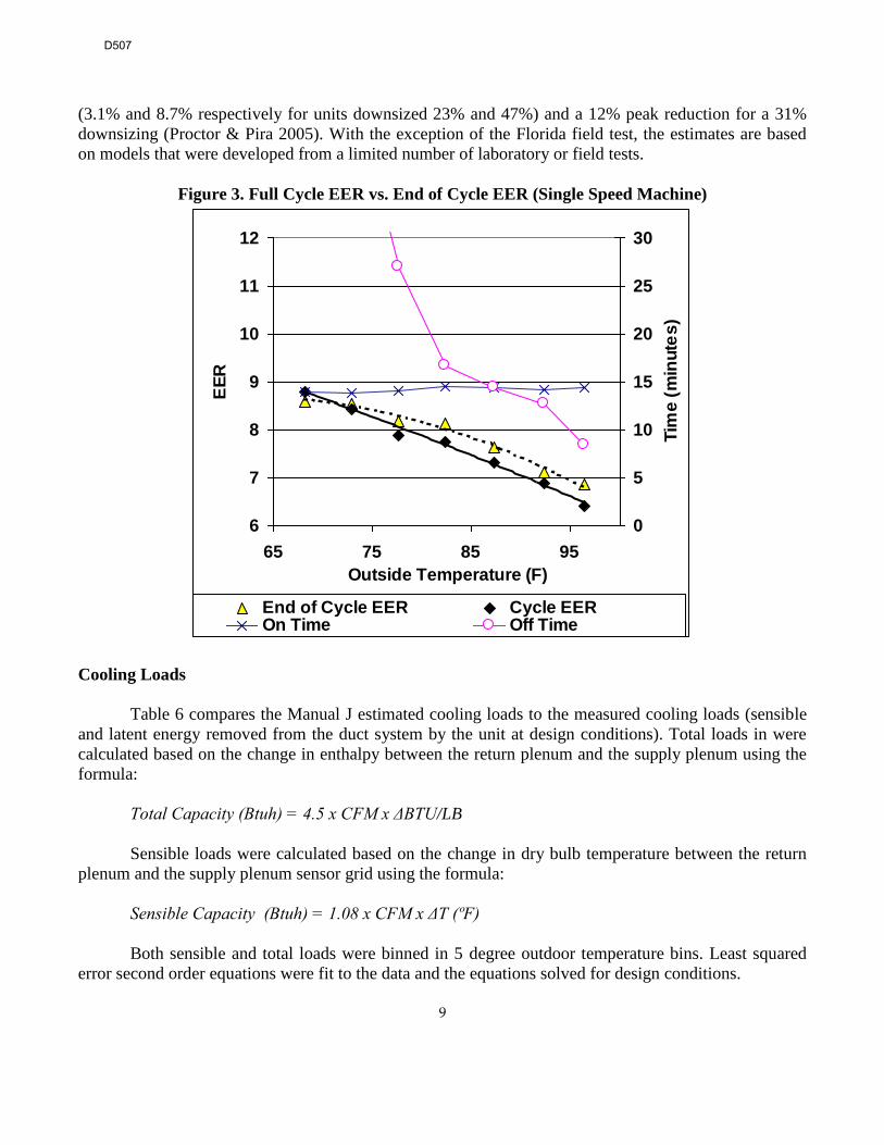
Single Speed Unit. For the single speed machine (Site P), the 5% efficiency drop may be an indication
of a small potential savings from downsizing that unit. Figure 2 shows that the single speed (Site P)
cycling performance conforms closely to its steady state performance over a range of temperatures.
The results of oversizing single speed units are increased electrical peak and, in some cases,
insufficient dehumidification and increased energy consumption. Using a combined thermostat, air
conditioner, and building simulation model, one study estimated that an AC system oversized by 50%
would use 9% more energy than a properly sized system (Henderson 1992). A regression model based
on data from 308 of the Florida field test of 368 homes estimated energy penalties of 3.7% and 9.3%
respectively for units 20% and 50% oversized. In addition, homes with systems greater than 120% of
Manual J averaged 13% greater peak cooling electrical load than homes without oversized systems
(James et al. 1997). An empirical analysis of closely monitored units produced similar energy savings
D507
9
(3.1% and 8.7% respectively for units downsized 23% and 47%) and a 12% peak reduction for a 31%
downsizing (Proctor & Pira 2005). With the exception of the Florida field test, the estimates are based
on models that were developed from a limited number of laboratory or field tests.
Figure 3. Full Cycle EER vs. End of Cycle EER (Single Speed Machine)
6
7
8
9
10
11
12
65 75 85 95
Outside Temperature (F)
EE
R
0
5
10
15
20
25
30
Tim
e (
min
ute
s)
End of Cycle EER Cycle EEROn Time Off Time
Cooling Loads
Table 6 compares the Manual J estimated cooling loads to the measured cooling loads (sensible
and latent energy removed from the duct system by the unit at design conditions). Total loads in were
calculated based on the change in enthalpy between the return plenum and the supply plenum using the
formula:
Total Capacity (Btuh) = 4.5 x CFM x ΔBTU/LB
Sensible loads were calculated based on the change in dry bulb temperature between the return
plenum and the supply plenum sensor grid using the formula:
Sensible Capacity (Btuh) = 1.08 x CFM x ΔT (ºF)
Both sensible and total loads were binned in 5 degree outdoor temperature bins. Least squared
error second order equations were fit to the data and the equations solved for design conditions.
D507
10
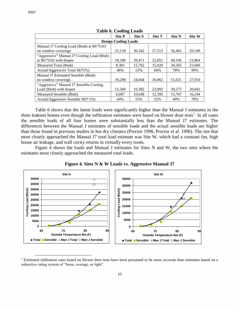
Table 6. Cooling Loads Site P Site S Site T Site N Site W
Design Cooling Loads
Manual J7 Cooling Load (Btuh) at 90/75/63
no window coverings 22,118 36,342 27,513 56,462 29,549
“Aggressive” Manual J7 Cooling Load (Btuh)
at 90/75/63 with drapes 18,180 29,471 22,851 44,106 23,864
Measured Total (Btuh) 8,381 15,702 15,026 34,565 23,660
Actual/Aggressive Total MJ7(%) 46% 53% 66% 78% 99%
Manual J7 Estimated Sensible (Btuh)
no window coverings 19,298 24,044 30,862 51,631 27,010
“Aggressive” Manual J7 Sensible Cooling
Load (Btuh) with drapes 15,360 19,382 23,992 39,275 20,841
Measured Sensible (Btuh) 6,687 10,648 12,395 15,767 16,244
Actual/Aggressive Sensible MJ7 (%) 44% 55% 52% 40% 78%
Table 6 shows that the latent loads were significantly higher than the Manual J estimates in the
three leakiest homes even though the infiltration estimates were based on blower door tests1. In all cases
the sensible loads of all four homes were substantially less than the Manual J7 estimates. The
differences between the Manual J estimates of sensible loads and the actual sensible loads are higher
than those found in previous studies in hot dry climates (Proctor 1998, Proctor et al. 1996). The site that
most closely approached the Manual J7 total load estimate was Site W, which had a constant fan, high
house air leakage, and wall cavity returns in virtually every room.
Figure 4 shows the loads and Manual J estimates for Sites N and W, the two sites where the
estimates most closely approached the measured total loads.
Figure 4. Sites N & W Loads vs. Aggressive Manual J7
1 Estimated infiltration rates based on blower door tests have been presumed to be more accurate than estimates based on a
subjective rating system of “loose, average, or tight”.
Site W
0
5000
10000
15000
20000
25000
30000
35000
65 75 85 95
Outside Temperature Bin (F)
Co
olin
g L
oa
d (
Btu
h)
Total Sensible Man J Total Man J Sensible
Site N
0
5000
10000
15000
20000
25000
30000
35000
40000
45000
65 75 85 95
Outside Temperature Bin (F)
Co
olin
g L
oa
d (
Btu
h)
Total Sensible Man J Total Man J Sensible
D507

11
Peak Energy Use
Peak watt draws between 4:00-5:00 pm and 5:00-6:00 pm are tabulated in Table 7 from the 10
cooling days with the highest power draw as well as the single day with the maximum power draw. In
this table, the input power is the average power in the given hour. The input power is less than the full
connected load if the unit cycles during the hour or if it runs on low speed for some part of the hour. The
worst-case scenario for utility peak demand is if the unit runs at connected load for the hour. This
adverse condition normally occurs when the delivered capacity of the air conditioner is less than the load
or when the occupants’ change the thermostat setting to a lower temperature. Large scale studies have
shown that, at peak, there are a group of homes (14% to 36%) running at full connected load, another
group of homes with the air conditioner cycling (44% to 85%) and a third group of homes with the air
conditioners not running at all (1% to 21%). The local mix of these groups determine the diversified
peak performance of air conditioners and the efficacy of measures designed to reduce peak (Peterson
and Proctor 1998).
Table 7. Summer Peak Demand Site P Site S Site T Site N Site W
Peak kW (10 highest)
4 to 5 PM Average Power (Wh/hr) 1592 2791 2631 2243 3439
4 to 5 PM Duty Cycle 66% 84% 100% 100% 100%
5 to 6 PM Average Power (Wh/hr) 1714 2517 2528 1058 3122
5 to 6 PM Duty Cycle 70% 79% 99% 53% 100%
Peak kW (single highest)
4 to 5 PM Average Power (Wh/hr) 1749 3490 2851 2674 3959
4 to 5 PM Duty Cycle 67% 80% 100% 100% 100%
5 to 6 PM Average Power (Wh/hr) 2709 2973 2647 2036 3855
5 to 6 PM Duty Cycle 97% 100% 100% 95% 100%
Connected Load (W at High Speed) 3225 4679 2820 4200 4390
One of the sites (Site T) fell into the full connected load group in the highest days. This was
caused by thermostat manipulation by the occupants. A second site (Site P) approached full connected
load only in the single highest peak day. These two units illustrate the potential peaking problem with
oversized single speed machines.
All the units that were operating as true dual-stage machines (S, N, and W) operated at less than
full connected load, switching between high and low speed, during the peak hours.
Seasonal Efficiency
Seasonal Energy Efficiency and consumption were calculated using TMY-2 temperature bins for
locations selected for proximity, similar latitude, and similar distance inland. The capacities and input
powers were averaged for all cycles in each temperature bin for Seasonal Efficiency calculations. Each
site is compared to average central air conditioned homes in the Middle Atlantic region by AC Energy
Intensity [kWh/sq.ft.] (EIA 2001). The results of that analysis are shown in Table 8.
D507

12
Table 8. Seasonal Energy Efficiency and Consumption Site Site P
1 Site S Site T Site N Site W
Seasonal Performance
Rated SEER 14.25 14 15 14 14
Measured Seasonal BTU/Wh 7.92 8.6 11.5 11.7 8.25
Seasonal BTU/Wh without constant fan 9.9 12.2
Seasonal kWh 1445 2351 2777 2168 1870
Seasonal kWh without constant fan 1986 1299
Average Seasonal kWh/sq.ft. in Region 0.63 0.63 0.63 0.63 0.63
Site Seasonal kWh/sq.ft. 0.89 0.99 1.46 0.62 0.81
1. ARI ratings are not available for the system combination (using a third party evaporator coil). The estimated rated SEER,
EER, power, and capacities are for a manufacturer’s combination with the same nominal capacity.
In all cases the seasonal efficiency was less than the rated SEER. Sites S and W would both be
substantially more efficient without the continuous fan. All homes except Site N had an AC Energy
Intensity (seasonal air conditioning kWh per conditioned square foot) that exceeded the average for the
Mid Atlantic Region (EIA 2001).
Site P The calculated seasonal efficiency based on the TMY-2 data in combination with the
monitored data is 7.92, which is 53% of the rated SEER of 14.25. One reason for the large discrepancy
may be the use of an aftermarket evaporator coil with an inferred rating.
Uncertainty
Sources of uncertainty in the analysis include the airflow, air temperature measurement,
humidity measurement, and electrical power measurement. Confidence in temperature rise and
electrical power measurements is high. Humidity and airflow measurements are the largest sources of
uncertainty.
Estimated supply and return air temperature measurement accuracy is ± 1°F. The supply/return
air differential was calibrated to less than 1°F. Electrical power was measured with Ohio Semitronics
watt-hour transducer rated as accurate to 2%. The relative humidity sensors have a rated accuracy of ±
2% for relative humidity between 10% and 90%. Relative humidity in the supply plenum often
approaches 100% and is difficult to measure accurately. We estimate our supply humidity measurements
to be accurate to ± 4%, not including the effect of response time. Airflow was measured with Energy
Conservatory’s True Flow® flow grid. The flow grid is rated as accurate to within 8%.
We estimate the confidence interval in the total capacity and efficiency statistics at about ±15%.
We estimate the confidence interval in sensible capacity and efficiency statistics at about ±10%. We
estimate the confidence interval in the energy consumption at about ± 2%.
D507
13
Summary and Conclusions
Site N, the 1960s 3500 square foot home, was the best performing home from an energy and
peak perspective. This home had a constant thermostat setting. It also had the second highest air leakage
and, as a result, the properly sized, dual-stage, variable blower speed air conditioner with instant fan off
was unable to adequately control the moisture in the home.
This home had the smallest capacity air conditioner per square foot and per measured cooling
load. Nevertheless the air conditioner was still sufficiently oversized that it operated on a combination of
high and low speed during peak hours. This site also had the most efficient unit turning in a cycle
efficiency of 15 Btu/Wh in the 80ºF to 85ºF temperature bin. This cycle efficiency is 99% of the actual
low speed EER and 95% of the manufacturer’s rating.
Site P, the single speed machine has performance inconsistent with other single speed ACs field
monitored by the authors (Proctor 1998, 5). Field monitored efficiencies for single speed air conditioners
with proper charge and airflow generally perform within a few percent of the manufacturers’ published
data2. The EER of this unit was only 64% of the rating in the 80 ºF to 85 ºF temperature bin.
The two sites (S and T) with constant fan display a variety of problems expected with that type
of fan control (Shirey, Henderson, & Raustad 2006). The seasonal energy efficiencies of these two units
were substantially degraded, the cycling efficiencies were low compared to their end of cycle
efficiencies, and the dehumidification was compromised.
The two sites (N and W) with the leakiest building shells had excessive indoor humidity that was
not adequately controlled by the air conditioners. It is likely that Site W had significant duct leakage
which, when combined with constant fan, exacerbated the humidity problems.
The dual-stage units with instant fan off or slightly delayed fan off showed little cycling
degradation indicating that reduced AC sizing may have little effect on the seasonal energy
consumption. In fact there is a concern that reducing the size of these units would cause them to run at
their less efficient high speed more of the time and increase both energy consumption and peak watt
draw.
The design conditions sensible loads at every site were between 40% and 78% of the Manual J
estimates. On the other hand, the latent loads at the three leakiest buildings were higher than the Manual
J estimates.
The dual-stage units were producing actual seasonal energy efficiency ratios between 59% and
84% of their rated SEERs. In addition, all the sites used a more cooling kWh per square foot than the
EIA published average for the Middle Atlantic Region. The Energy Star rated home was the next to
worst performing home of the group based on air conditioner electrical consumption intensity.
2 When the manufacturers’ published data are corrected for actual fan watt draws.
D507
14
References
[EIA] Energy Information Administration. 2001. Electric Air-Conditioning Energy Consumption in US
Households by Northeast Census Region. Available online:
http://www.eia.doe.gov/emeu/recs/recs2001/ce_pdf/aircondition/ce3-9c_ne_region2001.pdf.
Washington, P.C.: Energy Information Administration.
Henderson, H. 1992. “Dehumidification at Part Load.” In ASHRAE Transactions, Vol.98, Part 1, 370-
380, 3579. Atlanta, Georgia: American Society of Heating Refrigeration and Air-Conditioning
Engineers.
James, P., J.E. Cummings, J. Sonne, R. Vieira, J. Klongerbo. 1997. “The Effect of Residential
Equipment Capacity on Energy Use, Demand, and Run-Time.” In ASHRAE Transactions, Vol 103,
Pt. 2. Atlanta, Georgia.: American Society of Heating, Refrigerating, and Air- Conditioning
Engineers.
Peterson, G. and J. Proctor. 1998. “Effects of Occupant Control, System Parameters, and Program
Measures on Residential Air Conditioner Peak Loads.” In Proceedings from the ACEEE 1998
Summer Study on Energy Efficiency in Buildings, 1:253-264. Washington, D.C.: American Council
for and Energy-Efficient Economy.
Proctor, J. 1998. “Monitored In-Situ Performance of Residential Air-Conditioning Systems.” In
ASHRAE Transactions, Vol.104, Part 1. SF-98-30-4. Atlanta, Georgia: American Society of Heating
Refrigeration and Air-Conditioning Engineers.
Proctor, J., M. Blasnik, T. Downey, J. Sundal, and G. Peterson 1996. 1995 Update – Assessment of
HVAC Installations in Nevada Power Company Service Territory. EPRI Report TR-105309 Palo
Alto, California: Electric Power Research Institute.
Proctor, J., G. Cohn, and A. Conant 2006. The Heating and Cooling Performance of High Efficiency
HVAC Systems in the Northeast. 01.118. San Rafael, California.: Proctor Engineering Group.
Proctor, J. and J. Pira. 2005. System Optimization of Residential Ventilation, Space Conditioning and
Thermal Distribution. ARTI-21CR/611-30060-01. Arlington, Virginia.: Air-Conditioning and
Refrigeration Technology Institute.
Shirey, D.B., H.I. Henderson, and R.A. Raustad. 2006. Understanding the Dehumidification
Performance of Air-Conditioning Equipment at Part-Load Conditions. FSEC-CR-1537-05. Cocoa,
Florida.: Florida Solar Energy Center.
Acknowledgements
The authors would like to acknowledge the efforts of Lou Marrongelli and the entire
Conservation Services Group Crew, Elizabeth Titus, the project manager from the Northeast Energy
Efficiency Partnerships, as well as the sponsors of this project: DOE, New Jersey Board of Public
Utilities, and New York State Energy Research and Development Authority.
D507