Two-Sided Learning and the Ratchet Principle

Gonzalo Cisternas∗

MIT Sloan

February 2017

Abstract

I study a class of continuous-time games of learning and imperfect monitoring. A long-

run player and a market share a common prior about the initial value of a Gaussian hidden

state, and learn about its subsequent values by observing a noisy public signal. The long-

run player can nevertheless control the evolution of this signal, and thus affect the market’s

belief. The public signal has an additive structure, and noise is Brownian. I derive conditions

for a solution to an ordinary differential equation to characterize behavior in which the long-

run player’s equilibrium actions depends on the history of the game only through the market’s

correct belief. Using these conditions, I demonstrate the existence of equilibria in pure strategies

for settings in which the long-run player’s flow utility is nonlinear. The central finding is a

learning-driven ratchet principle affecting incentives. I illustrate the economic implications of

this principle in applications to monetary policy, earnings management, and career concerns.

Keywords: learning, private beliefs, ratchet effect, Brownian motion.

JEL codes: C73, D82, D83.

1 Introduction

Hidden variables are at the center of many economic interactions: firms’ true fundamentals

are hidden to both managers and shareholders; workers’ innate abilities are unobserved by

both employers and workers themselves; and growth and inflation trends are hidden to both

∗Email: gcistern@mit.edu. Earlier versions of this paper were circulated under the title “Two-SidedLearning and Moral Hazard.” I would like to thank Yuliy Sannikov for his invaluable advice, and Dilip Abreu,Alessandro Bonatti, Hector Chade, Eduardo Faingold, Bob Gibbons, Leandro Gorno, Tibor Heumann,Andrey Malenko, Ivan Marinovic, Stephen Morris, Marcin Peski, Juuso Toikka, Larry Samuelson, MikeWhinston and audiences at Columbia, Harvard-MIT, MIT Sloan, NYU Stern, Stanford GSB, ToulouseSchool of Economics, UCLA, UCSD and the University of Minnesota for their feedback. Also, I would liketo thank three anonymous referees for very valuable suggestions that helped improve the paper.

1

policymakers and market participants. In those settings, economic agents face common

uncertainty regarding payoff-relevant states that underlie the economic environment, and

eliminating such uncertainty can be prohibitively costly, or simply impossible; agents thus

learn about such states simultaneously as decisions are being made, and the incomplete

information they face need not ever disappear. This paper is concerned with examining

strategic behavior in settings characterized by such forms of fundamental uncertainty.

When agents learn about economic environment, behavior can be influenced the possibil-

ity of affecting the beliefs of others. The set of questions that can be asked in such contexts

is incredibly rich. In financial markets, is it possible for markets to hold correct beliefs about

firm’s fundamentals in the presence of earnings management? In labor markets, what are the

forces that shape workers’ incentives when they want to be perceived as highly skilled? In

policy, how is a central bank’s behavior shaped by the possibility of affecting markets’ beliefs

about the future evolution of inflation? The challenge in answering these questions lies on

developing a framework that is tractable enough to accommodate both Bayesian updating

to capture ongoing learning, and imperfect monitoring to capture strategic behavior.

To make progress towards the understanding of games of learning and imperfectly observ-

able actions, I employ continuous-time methods using Holmstrom’s (1999) signal-jamming

technology as the key building block. In the setting I study, there is a long-run player and

a market (i.e., a population of small individuals) who, starting from a common prior, learn

about an unobserved Gaussian fundamentals process by observing a public signal. The long-

run player can nevertheless influence the market’s belief about the fundamentals by taking

unobserved actions that affect the evolution of the publicly observed state. As in Holmstrom

(1999), actions and the fundamentals are perfect substitutes in the signal technology, and

thus the long-run player cannot affect the informativeness of the public signal (i.e., there is

no experimentation). Using Brownian information, I study Markov equilibria in which the

long-run player’s behavior depends on the history through the belief about the hidden state.

In an equilibrium in pure strategies, the market must anticipate the long-run player’s

actions at all times; beliefs thus coincide on the equilibrium path. However, allowing for belief

divergence is critical to determine the actions that arise along the path of play. Consider,

for instance, the earnings management example. To show that an equilibrium in which the

market holds a correct belief exists, it must be verified that the payoff that the manager

obtains by reporting earnings as conjectured by the market dominates the payoff under any

other strategy. But if the manager deviates, the market will misinterpret the report; at those

off-path histories, both parties’ beliefs about the firm’s fundamentals differ.

Crucially, when actions are hidden, deviations from the market’s conjectured behavior

lead the long-run player’s belief to become private. Moreover, this private information is

2

persistent, as it comes from a learning process. As I will explain shortly, the combination

of hidden actions and private private information off the path of play severely complicates

the equilibrium analysis in virtually every setting that allows for learning and imperfect

monitoring with frequent arrival of information.1

To address this difficulty, I follow a first-order approach to studying Markov equilibria

in settings where (i) affecting the public signal is costly and (ii) the long-run player’s flow

payoff is a general—in particular, nonlinear—function of the market’s belief. Specifically, I

construct a necessary condition for equilibria in which on-path behavior is a differentiable

function of the common belief, and then provide conditions under which this necessary con-

dition is also sufficient. The advantages of this approach are both conceptual and technical.

First, the necessary condition uncovers the forces that shape the long-run player’s behavior

in any Markov equilibrium, provided that an equilibrium of this form exists. Second, this

approach offers a tractable venue for demonstrating the existence of such equilibria despite

the intricacies of off-path private beliefs affecting behavior.

Economic contribution. The main finding of this paper pertains to a ratchet principle

affecting incentives. Consider a manager who evaluates boosting a firm’s earnings report

above analysts’ predictions. The immediate benefit from this action is clear: abnormally high

earnings lead the market to believe that the firm’s fundamentals have improved. Crucially,

the manager understands that this optimism is incorrect, as the observation of high earnings

was a consequence of altering the report. He then anticipates that subsequent manipulation

will be required to maintain the impact on the firm’s value, as his private belief about the

firm’s fundamentals indicates that the firm would otherwise underperform relative to the

market’s expectations. Equally important, if the market expects firms with better prospects

to manage their earnings more aggressively, this underperformance can become even more

acute. In either case, exhibiting good performance results in a more demanding incentive

scheme to be faced tomorrow—i.e., a learning-driven ratchet principle emerges.2

In this paper, ratchet effects—implications on behavior of the ratchet principle just

described—do not relate to reduced incentives for information revelation, as in models with

ex ante asymmetric information (e.g., Laffont and Tirole, 1988): this is because the long-run

player is unable to affect the informativeness of the public signal, which implies that the

speed of learning is exogenous. Instead, these effects are captured in the form of distorted

levels of costly actions relative to some benchmarks. More generally, their appearance is

1Holmstrom’s original setting is unique in this respect, as the linearity in payoffs assumed in his modelmakes incentives independent of the value that beliefs may take.

2Weitzman (1980) refers to the ratchet principle as the “tendency of planners to use current performanceas a criterion in determining future goals” (p.302). In Section 3 I show how a market revising its expectationsabout future values of a public signal is in fact a target revision from the long-run player’s perspective.

3

the outcome of a fundamental tension between Bayesian updating and strategic behavior,

and hence, they are not exclusive to the case of a Gaussian hidden state. Specifically, since

beliefs are revised based on discrepancies between observed and expected signal realizations,

actions that lead to abnormally high signals are inherently costly from a dynamic perspec-

tive: by creating higher expectations for tomorrow’s signals, such actions require stronger

future actions to generate a sustained effect on beliefs.

Applications. I first revisit Holmstrom’s (1999) seminal model of career concerns, which is

a particular instance of linear payoffs within the class of games analyzed. In this context, I

show that the form of ratcheting previously described is embedded in the equilibrium that he

finds. Importantly, by precisely quantifying the strength of this force, I show how ratcheting

plays an important role in limiting the power of market-based incentives in the equilibrium

found by Holmstrom when learning is stationary in his model.

A key advantage of this paper is its ability to accommodate nonlinear flow payoffs, which

can be a defining feature of many economic environments. In an application to monetary

policy, I consider a setting in which a price index carries noisy information about both an

unobserved inflation trend and the level of money supply, and a central bank can affect

employment by creating inflation surprises. The central bank’s trade-off between output

and inflation is modeled via a loss function that is quadratic in employment (or output) and

money growth. In such a context, I show that the ratchet principle can induce a monetary

authority to exhibit a stronger commitment to low inflation. Intuitively, while unanticipated

inflation can be used to boost employment in the short run, it also leads the market to

overestimate future inflation and, hence, to set excessively high nominal wages. This in

turn puts downward pressure on future hiring decisions, which makes inflation more costly

compared to settings in which the inflation trend is observed or simply absent.

Finally, I study more subtle ratchet effects in an application that analyzes managers’

incentives to boost earnings when they have a strong short-term incentive to exceed a zero-

earnings threshold, captured in marginal flow payoffs that are single-peaked and symmetric

around that point. In such a context, I show that firms that expect to generate positive

earnings can inflate reports more actively than firms at, or below, the threshold, despite

their managers having weaker myopic incentives and being unable to affect firms’ market

values. Intuitively, the market anticipates that successful manipulation by firms with poor

(good) past performance will lead to stronger (weaker) myopic incentives in the future.

Anticipating higher expectations of earnings management by the market, firms with poor

profitability find it more costly to inflate earnings relative their successful counterparts. The

distortion thus takes the form of a profile of manipulation that is skewed towards firms that

have exhibited better performances in the past.

4

Technical contribution. In the class of games analyzed, learning is conditionally Gaussian

and stationary, and hence, beliefs can be identified with posterior means. Moreover, a

nonlinear version of the Kalman filter applies. It is then natural to look for Markov perfect

equilibria (MPE) using standard dynamic programming tools, with the market and long-run

player’s beliefs as states. However, the combination of hidden actions and hidden information

off the path of play results in the long-run player’s value function no longer satisfying a

traditional Hamilton-Jacobi-Bellman (HJB) equation. In fact, the differential equation at

hand does not even have the structure of a usual partial differential equation (PDE); to the

best of my knowledge, no existence theory applies.

Implicit in the HJB approach is that, by demanding the determination of the long-run

player’s full value function, the method requires exact knowledge of the long-run player’s

off-path behavior to determine the actions that arise along the path of play; however, the

difficulty at hand is precisely that the long-run player can condition his actions on his private

information in complex ways as his own belief changes. Exceptions are settings in which the

long-run player’s flow payoff is linear in the market’s belief (e.g., Holmstrom, 1999), as in

those cases the long-run player’s optimal behavior is independent of the past history of play.

However, it is exactly in those linear environments that the differential equation delivered by

the HJB approach has a trivial solution. If the goal is then to analyze settings that naturally

involve nonlinearities, solution methods for linear environments do not apply.

The technical advantage of the first-order approach is that the ratcheting equation—the

necessary condition for equilibrium behavior—makes bypassing the exact computation of off-

path payoffs possible. In fact, this ordinary differential equation (ODE) offers a method to

guess for Markov equilibria without knowing how exactly the candidate equilibrium might be

supported off the path of play. Importantly, provided that it is verified that a deviation from

a solution to the ratcheting equation is not profitable, leaving off-path behavior unspecified in

the equilibrium concept is no disadvantage: equilibrium outcomes (i.e., actions and payoffs)

are determined exclusively by the actions prescribed by strategies along the path of play.

Therefore, for sufficiency, instead of computing off-path payoffs exactly, I approximate

them. Specifically, building on the optimal contracting literature, I bound off-path payoffs

in a way that parallels sufficiency steps in relaxed formulations of principal-agent problems

(Williams, 2011; Sannikov, 2014) to derive a verification theorem for Markov equilibria (The-

orem 1). The theorem involves the ratcheting equation and the ODE that characterizes the

evolution of the (candidate, on-path) payoff that results from inducing no belief divergence,

i.e., two ODEs rather than a PDE. The key requirement is that the information rent—a mea-

sure of the value of acquiring private information about the continuation game—associated

with the solution of the system at hand cannot change too quickly.

5

The advantage of this verification theorem—relative to both the HJB approach and

the contracting literature—is its tractability. Using this result, I determine conditions on

primitives that ensure the existence of Markov equilibria in two classes of games exhibiting

nonlinearities: linear quadratic games and games with bounded marginal flow payoffs (The-

orems 2 and 3), which host the applications I examine. These three results address the belief

divergence challenge, and the continuous-time approach is critical for their derivation.

Related literaure. Regarding the literature on the ratchet effect, Weitzman (1980) illus-

trates how revising production targets on the basis of observed performance can dampen

incentives in planning economies; both the incentive scheme and the revision rule are exoge-

nous in his analysis. Freixas et al. (1985) and Laffont and Tirole (1988) in turn endogenize

ratcheting by allowing a principal to optimally revise an incentive scheme as new information

about an agent’s hidden type is revealed upon observing performance; the main result is that

there is considerable pooling.3 As in Weitzman (1980), my analysis focuses on the size of

equilibrium actions, rather than on their informativeness. In line with the second group of

papers, the strength of the ratcheting that arises in any specific setting is an equilibrium

object: by conjecturing the long-run player’s behavior, the market effectively imposes an

endogenous moving target against which the long-run player’s performance is evaluated.

Concurrently with this paper, Bhaskar (2014), Prat and Jovanovic (2014), and Bhaskar

and Mailath (2016) identify ratchet principles in principal-agent models with symmetric

uncertainty: namely, that good performance can negatively affect an agent’s incentives if it

leads a principal to overestimate a hidden technological parameter. My analysis differs from

these papers along two dimensions. First, I show that market-based incentives can lead to

quite rich behavior on behalf of a forward-looking agent; instead, the contracts that these

papers analyze implement either minimal or maximal effort. Second, I show that, in games

of symmetric uncertainty, the ratchet principle is also determined by a market revising its

expectations of future behavior, in addition to revising its beliefs about an unobserved state.4

This paper belongs to a broader class of games of ex ante symmetric uncertainty in

which imperfect monitoring leads to the possibility of divergent beliefs. In the reputation

literature, Holmstrom (1999) finds an equilibrium in which a worker’s equilibrium effort

is identical on and off the path of play, in part consequence of the assumed linearity in

payoffs.5 In Board and Meyer-ter-Vehn (2014), private beliefs matter non-trivially for a firm’s

3See Chapter 9 in Laffont and Tirole (1993) for an excellent summary.4Also in the context of symmetric uncertainty, Meyers and Vickers (1997) study a model of regulation

in which ratcheting is modeled explicitly via an exogenous incentive scheme that reduces payments to moreefficient firms. Martinez (2009) instead identifies the potential appearance of endogenous ratchet-like forcesin a model of career concerns with piecewise linear wages.

5Kovrijnykh (2007), Martinez (2006, 2009) and Bar-Isaac and Deb (2014) study nonlinearities in models

6

investment policy, and the existence of an equilibrium is shown via fixed-point arguments; my

approach is instead constructive and focused on pure strategies. Private beliefs also arise in

strategic experimentation settings involving a risky arm of two possible types and perfectly

informative Poisson signals. Since beliefs are deterministic in this case, the equilibrium

analysis is tractable (Bergemann and Hege (2005) derive homogeneity properties of off-path

payoffs and Bonatti and Horner (2011, 2016) apply standard optimal control techniques),

and the ratcheting I find is absent, as the observation of a signal terminates the interaction.

To conclude, this paper contributes to a growing literature that analyzes dynamic in-

centives exploiting the tractability of continuous-time methods. Sannikov (2007), Faingold

and Sannikov (2011) and Bohren (2016) study games with imperfect monitoring in which

the continuation game is identical on and off the equilibrium path. In contrast, as in the

current paper, in the principal-agent models of Williams (2011), Prat and Jovanovic (2014),

and Sannikov (2014), deviations lead the agent to obtain private information about future

output. All these contracting papers derive measures of information rents and general suffi-

cient conditions that validate the first-order approach they follow. Such sufficient conditions

involve endogenous variables, and their verification is usually done both ex post (i.e., using

the solution to the relaxed problem) and in specific settings. The sufficient conditions that

I derive can be instead mapped to primitives for a large class of economic environments.

1.1 Outline

Section 2 presents the model and Section 3 derives necessary conditions for Markov equilibria.

Section 4 explores applications. Section 5 states the verification theorem, and Section 6

contains the existence results. Section 7 concludes. All proofs are relegated to the Appendix.

2 Model

A long-run player and a population of small players (the market) learn about a hidden state

(θt)t≥0 (the fundamentals) by observing a public signal (ξt)t≥0. Their evolution is given by

dθt = −κ(θt − η)dt+ σθdZθt , t > 0, θ0 ∈ R, (1)

dξt = (at + θt)dt+ σξdZξt , t > 0, ξ0 = 0. (2)

In this specification (Zθt )t≥0 and (Zξ

t )t≥0 are independent Brownian motions, and σθ and

σξ are strictly positive volatility parameters. The fundamentals follow a Gaussian diffusion

of career concerns with finite horizon. Except in the two-period model of Bar-Isaac and Deb (2014), wheresufficiency reduces to static second-order conditions, the question of existence of equilibria is not addressed.

7

(hence, Markov) process where κ ≥ 0 is the rate at which (θt)t≥0 reverts towards the long-run

mean η ∈ R.6 The public signal (2) carries information about the fundamentals in its drift,

but it is affected by the long-run player’s choice of action at, t ≥ 0. These actions take values

in an interval A ⊆ R, with 0 ∈ A, and they are never directly observed by the market.

The monitoring technology (2) is the continuous-time analog of Holmstrom’s (1999)

signal-jamming technology, and a key property of it is that it satisfies the full-support as-

sumption with respect to the long-run player’s actions.7 Thus, the only information that the

market has comes from realizations of (ξt)t≥0; let (Ft)t≥0 denote the corresponding public

filtration, and ξt := (ξs : 0 ≤ s ≤ t) any realized public history.

I will examine equilibria in pure strategies in which the long-run player’s behavior along

the path of play is, at all instants of time, a function of the current public history ξt, t ≥ 0.

The formal notion of a pure public strategy for the long-run player is defined next; I refer to

any such pure public strategy simply as a strategy thereafter.

Definition 1. A (pure public) strategy (at)t≥0 is a stochastic process taking values in A that

is, in addition, progressively measurable with respect to (Ft)t≥0, and that satisfies E[´ t

0a2sds]<

∞, t ≥ 0. A strategy is feasible if, in addition, (2) admits a unique solution.8

Everyone shares a prior that θ0 is normally distributed, with a variance γ∗ that ensures

that learning is stationary—in this case, the Gaussian structure of both the fundamentals

and noise permits posterior beliefs to be identified with posterior means; I defer the details

to Section 3.1. Crucially, in order to interpret the public signal correctly, the market needs

to conjecture the long-run player’s equilibrium behavior; in this way, the market can account

for how the latter agent’s actions affect the evolution of the public signal. Thus, let

p∗t := Ea∗ [θt|Ft]

denote the mean of the market’s posterior belief about θt given the information up to time

t ≥ 0 under the assumption that the feasible strategy (a∗t )t≥0 is being followed. In what

6When κ = 0, (θt)t≥0 corresponds to a Brownian martingale. In the κ 6= 0 case, this process is usuallyreferred to as an Ornstein-Uhlenbeck (or mean-reverting) process.

7This is a consequence of Girsanov’s theorem, which states that changing the drift in the public signalinduces an equivalent distribution over the set of paths of (ξt)t≥0.

8Formally, the game takes place in the following filtered probability space (Ω, (Ft)t≥0,P) (for referenceC(E) denotes the set of continuous functions from E ⊆ R to R): (i) Ω = C(R+) is the set of sample pathsof (ξt)t≥0; (ii) Ft is the canonical σ-algebra on C([0, t]); and (iii) P is the probability measure on C(R+)induced by the long-run player’s equilibrium actions via (2). The solution concept for (2) is in a weaksense, i.e., there exists a probability distribution on C(R+) that is consistent with (2) under (at)t≥0, and theuniqueness requirement on such probability distribution ensures that the outcome of the game is uniquelydefined. A strategy is thus a function a : R+ × C(R+) → A, i.e., a mapping connecting (t, ξ)-pairs withactions. Progressive measurability implies that at(ξ) depends only on ξt, t ≥ 0, (i.e., (at)t≥0 is adapted to(Ft)t≥0). Finally, the integrability condition suffices for standard filtering equations to hold.

8

follows, the market’s conjecture (a∗t )t≥0 is fixed, and I refer to the corresponding posterior

mean process (p∗t )t≥0 as the public belief process.

The market behaves myopically given its beliefs about the fundamentals and equilibrium

play.9 Specifically, there is a measurable function χ : R × A → R such that, at each time

t, the market takes an action χ(p∗t , a∗t ) that affects the long-run player’s utility. As a result,

the total payoff to the long-run player of following a feasible strategy (at)t≥0 is given by

U(p) := Ea[ˆ ∞

0

e−rt(u(χ(p∗t , a∗t ))− g(at))dt

∣∣∣p0 = p

], (3)

where p0 = p denotes the prior mean of θ0. In this specification, the notation Ea[·] emphasizes

that a strategy (at)t≥0 induces a distribution over the paths of (ξt)t≥0, thus affecting the

likelihood of any realization of (p∗t )t≥0. Also, u : R → R is measurable, and r > 0 denotes

the discount rate. Finally, affecting the public signal is costly according to a convex function

g : A→ R+ such that g(0) = 0, g′(a) > 0 for a > 0, g′(a) < 0 for a < 0 (i.e., increasing the

rate of change of the public signal in either direction is costly at increasing rates).

Mild technical conditions on u, χ and g that are used for studying equilibria characterized

by ODEs are presented next—these conditions are not needed for examining pure-strategy

equilibria at a general level (Definition 2 below), and they are discussed at the end of this

section (Remark 1). Let Ck(E;F ) be the set of k-times differentiable functions from E ⊂ Rn

to F ⊂ R, n ≥ 1, with a continuous k-th derivative; I omit k if k = 0, and F if F = R.

Assumption 1. (i) Differentiability: u ∈ C1(R), χ ∈ C1(R× A) and g ∈ C2(A;R+) with

ρ := (g′)−1 ∈ C2(R).

(ii) Growth conditions: the partial derivatives χp and χa∗ are bounded in R × A, and u, u′

and g′ have polynomial growth.10 (iii) Strong convexity: g′′(·) ≥ ψ for some ψ > 0.11

As is standard in stochastic optimal control, a strategy (at)t≥0 is admissible for the long-

run player if it is feasible and

Ea[ˆ ∞

0

e−rt|u(χ(p∗t , a∗t ))− g(at)|dt

∣∣∣ p0 = p

]<∞,

9The market can correspond to a sequence of short-run players, or a continuum of identical forward-looking agents who only maximize ex ante flow payoffs over [t, t + dt). The latter can occur if, in the(unmodeled) game played amongst them, each agent is unable to affect any payoff-relevant state.

10f : R→ R is said to have polynomial growth if there is C > 0 and j ∈ N such that |f(p)| ≤ C(1 + |p|j)for all p ∈ R. When j = 2 (j = 1) it is said that f has quadratic (linear) growth.

11A quadratic cost function satisfies all the conditions on g(·).

9

(cf., Pham, 2009). In this case, it is said that (at, a∗t )t≥0 is an admissible pair.

Definition 2. A strategy (a∗t )t≥0 is a pure-strategy Nash equilibrium (NE) if (a∗t , a∗t )t≥0 is

an admissible pair and

(i) (a∗t )t≥0 maximizes (3) among all strategies (at)t≥0 such that (at≥0, a∗t )t≥0 is an admis-

sible pair, and

(ii) (p∗t )t≥0 is constructed via Bayes’ rule using (a∗t )t≥0.

In a (pure-strategy) NE, the long-run player finds it optimal to follow the market’s

conjecture of equilibrium play while the market is simultaneously using the same strategy

to construct its belief. Thus, along the path of play, (i) the long-run player’s behavior

is sequentially rational, and (ii) the long-run player and the market hold the same belief

at all times. Allowing for belief divergence is, nevertheless, a critical step towards the

determination of the actions that arise along the path of play, and at those off-path histories

the long-run player can condition his actions on more information than that provided by

the public signal; Sections 3 and 5 are devoted to this equilibrium analysis. It is important

to stress, however, that for the analysis of equilibrium outcomes (i.e., actions and payoffs),

leaving behavior after deviations unspecified in the equilibrium concept is without loss, as

the full-support monitoring structure (2) makes this game one of unobserved actions.12

The focus is on equilibria that are Markov in the public belief with the property that

actions are interior, and the corresponding policy (i.e., the mapping between beliefs and

actions) and payoffs exhibiting enough differentiability, as defined next:

Definition 3. An equilibrium is Markov if there is a∗ ∈ C2(R; int(A)) Lipschitz such that

(a∗(p∗t ))t≥0 (with p∗t the common belief at t ≥ 0) is a NE, and U(p) ∈ C2(R).

In a Markov equilibrium, behavior depends on the public history only through the com-

mon belief according to a sufficiently differentiable function—such equilibria are natural to

analyze due to both the Markovian nature of the fundamentals and the presence of Brownian

noise. Importantly, the long-run player’s realized actions are, at all time instants, a function

of the complete current public history ξt via the dependence of p∗t on ξt (i.e., a∗t = a∗(p∗t [ξt])).

Moreover, if a∗(·) is nonlinear, such path dependence will also be nonlinear.

The rest of the paper proceeds as follows. Necessary and sufficient conditions for Markov

equilibria given a general best response χt := χ(p∗t , a∗t ), t ≥ 0, are stated in Sections 3 and

12Since the market cannot detect deviations, its information sets are indexed by the partial realizationsof the public signal. Thus, along the path of play of any equilibrium in which the market’s belief is correct,actions are a function of the current public history. But since all such sets are reached from a time-zeroperspective, it follows that the Nash equilibrium concept suffices to characterize the outcome of the game.

10

5, respectively. The applications that employ nonlinear flow payoffs (Sections 4.2 and 4.3)

and the existence results (Section 6) in turn specialize on the case χt = χ(p∗t ); as argued in

Section 3, this restriction is the natural one for studying traditional ratchet effects.

Remark 1 (On MPE). Any Markov equilibrium can be extended to MPE (with the market’s

and the long-run player’s belief as states) provided an off-path Markov best response exists;

the hurdle for showing such existence result is only technical, as the equilibrium analysis I

perform does not restrict the long-run player’s behavior off the path of play.13 Importantly,

if a MPE exists and the value function is of class C2, the associated policy when beliefs are

aligned in fact coincides with the policy of a Markov equilibrium (Remark 6, Section 5).

Remark 2 (On Assumption 1 and the Lipschitz property). The differentiability and growth

conditions in Assumption 1 are used to obtain necessary conditions for Markov equilibria

in the form of ODEs. On the other hand, the strong convexity assumption on g(·) permits

the construction of Lipschitz candidate equilibria using solutions to such ODEs. The Lips-

chitz property in turn guarantees that the long-run player’s best-response problem (via the

market’s conjecture of equilibrium play) is well defined in the sufficiency step. All these con-

ditions can be relaxed, but the extra generality brings no new additional economic insights.

3 Equilibrium Analysis: Necessary Conditions

To perform equilibrium analysis, one has to consider deviations from the market’s conjecture

of equilibrium behavior and show that they are all unprofitable. After a deviation occurs,

however, there is belief divergence, and long-run player’s belief becomes private. As I show in

Section 5, the combination of hidden actions and persistent hidden information off the path

of play leads traditional dynamic-programming methods to become particularly complex

when the task is to find MPE.

In order to bypass this complexity, I take a first-order approach to performing equilibrium

analysis in the Markov case. First, I derive a necessary condition for Markov equilibria:

namely, if deviating from the market’s conjecture is not profitable, the value of a small

degree of belief divergence must satisfy a particular ODE (Section 3.2). Second, I establish

conditions under which a solution to this ODE makes the creation of any degree of belief

asymmetry suboptimal, thus validating the first-order approach (Section 5.2). Importantly,

this approach is critical for uncovering the economic forces at play.

13More precisely, the traditional approach to showing the existence of optimal (Markov) policies forstochastic control problems of infinite horizon is via HJB equations. However, for the class of games understudy, such HJB approach raises additional complexities relative to standard decision problems (Section 5).Observe, however, that such an off-path best response always exists in settings where the set of actions isfinite, and the horizon discrete and finite.

11

3.1 Laws of Motion of Beliefs and Belief Asymmetry Process

Standard results in filtering theory state that, given a conjecture (a∗t )t≥0, the market’s belief

about θt given the public information up to t is normally distributed (with a mean denoted

by p∗t ).14 In the case of the long-run player, he can always subtract—regardless of the

strategy followed—the effect of his action on the public signal to obtain dYt := dξt − atdt =

θtdt + σξdZξt , t ≥ 0. Since (θt, Yt)t≥0 is Gaussian, it follows that his posterior belief process

is also Gaussian; denote by (pt)t≥0 the corresponding mean process.

In order for learning to be stationary, I set the common prior to have a variance equal to

γ∗ = σ2ξ

(√κ2 + σ2

θ/σ2ξ − κ

)> 0.

In this case, both the market and the long-run player’s posterior beliefs about θt have vari-

ance γ∗ at all times t ≥ 0, and hence, (p∗t )t≥0 and (pt)t≥0 become their sufficient statistics,

respectively. Observe also that γ∗ is independent of both conjectured and actual play. In

fact, because of the additively separable structure of the public signal, a change in the

long-run player’s strategy shifts the distribution of the public signal without affecting its

informativeness, i.e., there are no experimentation effects.15

Lemma 1. If the market conjectures (a∗t )t≥0, yet (at)t≥0 is being followed, then

dp∗t = −κ(p∗t − η)dt+γ∗

σ2ξ

[dξt − (p∗t + a∗t )dt] and (4)

dpt = −κ(pt − η)dt+γ∗

σξdZt, t ≥ 0, (5)

where Zt := 1σξ

(ξt −´ t

0(ps + as)ds

)= 1

σξ

(Yt −

´ t0psds

), t ≥ 0, is a Brownian motion

from the long-run player’s perspective. Moreover, (ξt)t≥0 admits the representation dξt =

(at + pt)dt+ σξdZt, t ≥ 0, from his standpoint.

Proof: Refer to Theorems 7.12 and 12.1 in Liptser and Shiryaev (1977).

The right-hand side of (4) offers a natural orthogonal decomposition for the local evolution

of the public belief: the trend −κ(p∗t − η)dt, in the market’s time t-information set, plus the

14See Theorem 11.1 in Liptser and Shiryaev (1977). Formally, the pair (θt, ξt) is conditionally Gaussian,meaning that θt|Ft is normally distributed despite (ξt)t≥0 not being necessarily Gaussian. The latter occursif a∗t is a nonlinear function of (ξs)s<t, t ≥ 0, which can be in turn the result of a nonlinear Markov strategy.A nonlinear version of the Kalman-Bucy filter applies in this case.

15More generally, under a common normal prior with variance γo ≥ 0, Theorem 12.1 in Liptser andShiryaev (1977) shows that both posterior beliefs have a variance (γt)t≥0 that satisfies γt = −2κγt + σ2

θ −γ2t /σ

2ξ , t > 0, γ0 = γo, i.e., the speed of learning is exogenous. It is easy to verify that γ∗ is the unique

strictly positive stationary solution of this ODE.

12

residual ‘surprise’ process

dξt − Ea∗ [dξt|Ft] = dξt − (a∗t + p∗t )dt, (6)

which is unpredictable from the market’s perspective. Positive (negative) realizations of

this surprise process convey information that the fundamentals are higher (lower), and the

responsiveness of the public belief to this news is constant and captured by the sensitivity

β := γ∗/σ2ξ =

√κ2 + σ2

θ/σ2ξ − κ.16 (7)

In the absence of news, the market adjusts its beliefs at rate κ, i.e., in the same way that

the fundamentals change absent any shocks to their evolution.

The long-run player’s belief (pt)t≥0 has an analogous structure, with the Brownian motion

Zt = 1σξ

(ξt −´ t

0(ps + as)ds

)= 1

σξ

(Yt −

´ t0psds

)(or, equivalently, the surprise process σξZt)

now providing news about (θt)t≥0; the last equality stresses that the realizations of (Zt)t≥0

are independent of the strategy followed and, thus, that (pt)t≥0 is exogenous. In contrast, the

public belief is controlled by the long-run player through his actions affecting the surprise

term (6) via the realizations of (ξt)t≥0.

To see how deviations from (a∗t )t≥0 affect the public belief, Lemma 1 states that the public

signal follows dξt = (at + pt)dt+ σξdZt from the long-run player’s perspective. Plugging this

into (4), straightforward algebra yields that ∆t := p∗t − pt satisfies

d∆t = [−(β + κ)∆t + β(at − a∗t )]dt, t > 0, ∆0 = 0. (8)

It is clear from (8) that deviations from (a∗t )t≥0 can lead to belief asymmetry (∆ 6= 0): in this

case, the long-run player’s belief is private, as the correction dξt− atdt used to obtain dYt is

incorrectly anticipated by the market. In particular, an upward deviation on the equilibrium

path leads the market to hold an excessively optimistic belief about the fundamentals (i.e.,

∆t = p∗t − pt > 0), consequence of underestimating the contribution of the long-run player’s

action to the public signal. I refer to (∆t)t≥0 as the belief asymmetry process.

Starting from a common prior, however, beliefs remain aligned on the equilibrium path

(i.e., ∆0 = 0 and a∗t = at, t ≥ 0, imply ∆ ≡ 0). In particular, both parties expect any

surprise realization (6) to decay at rate κ on average along the path of play, as the common

belief evolves according to dpt = −κ(pt−η)dt+βσξdZt at any on-path history going forward

(see eqn. (5)).

16Thus, beliefs are less responsive to such news when κ, σξ and 1/σθ grow. In particular, higher ratesof mean reversion lead to a more concentrated long-run distribution of the fundamentals, and hence, to lessresponsiveness to news.

13

3.2 Necessary Conditions: The Ratcheting Equation

Consider the Markov case. In order to understand the form of ratcheting that arises in this

model, it is useful to interpret (ξt)t≥0 as a measure of performance (e.g., output) and the

market’s best response χ(·, ·) as a payment that rewards high performance. For expositional

simplicity, suppose that the long-run player is simply paid based on the market’s belief about

the fundamentals, χ(p∗, a∗) = p∗; this can occur if, for instance, the fundamentals reflect an

unobserved payoff-relevant characteristic of the long-run player (e.g., managerial ability).

In this case, the dynamic of the public belief (4) is effectively an incentive scheme, i.e., a

rule that determines how payments are revised in response to current performance:

dp∗t︸︷︷︸change in payments

= −κ(p∗t − η)dt︸ ︷︷ ︸exogenous trend

+ β︸︷︷︸sensitivity

× [ dξt︸︷︷︸performance

− (p∗t + a∗(p∗t ))dt︸ ︷︷ ︸target

].

Central to this scheme is the presence of a target in the form of expected performance: the

long-run player will positively influence his payment if and only if realized performance, dξt,

is above the market’s expectation, Ea∗ [dξt|Ft] = (p∗t + a∗(p∗t ))dt. But observe that the mar-

ket’s updated belief feeds into the target against which the long-run player’s performance is

evaluated tomorrow. Moreover, an upward revision of such target leads to a more demanding

incentive scheme to be faced in the future—a ratchet principle ensues.17

In continuous time, the distinction between today and tomorrow disappears. It is then

natural to define a ratchet as the (local) sensitivity of the performance target with respect

to contemporaneous realized performance dξt, namely,

Ratchet :=d(p∗t + a∗(p∗t ))

dξt=

[1 +

da∗(p∗)

dp∗

] ∣∣∣∣p∗=p∗t

× dp∗tdξt︸︷︷︸=β

= β + βda∗(p∗t )

dp∗.18 (9)

To understand the implications of this ratchet principle on incentives, consider the follow-

ing strategy (at)t≥0: the long-run player deviates from (a∗t )t≥0 for the first time at time t by

choosing at > a∗t , and he then matches the market’s expectation of performance thereafter.

Intuitively, this deviation helps illustrate the strength of the dynamic cost of exhibiting high

performance through quantifying the extra effort cost that the long-run player must bear to

17The way in which the public belief (4) is written (i.e., with (p∗t +a∗(p∗t ))dt displayed as a target, or with−β(p∗t+a

∗(p∗t )) in the drift) is immaterial: the point is that, to defeat or accelerate the natural reversion to themean, dξt must be greater than (p∗t+a∗(p∗t ))dt, and the same logic follows. Also, specializing to χ(p∗, a∗) = p∗

is without loss. In fact, dZ∗t := [dξt−(p∗t +a∗(p∗t ))dt]/σξ is a Brownian motion from the market’s perspective,so, using Ito’s rule, (χ(p∗t , a

∗(p∗t )))t≥0 has innovations also driven by dξt − (p∗t + a∗(p∗t ))dt.18This notion of sensitivity is with respect to realizations of (ξt)t≥0, and such realizations are driven by

(θt)t≥0 (not by (p∗t )t≥0). See remark 3 for more details on this sensitivity.

14

avoid disappointing the market after strategically surprising the latter.

Matching the market’s expectation of performance at all times after a deviation occurs

amounts to equating the drift of (ξs)s>t from the market’s perspective. Thus, the long-run

player must take actions according to

as + ps︸ ︷︷ ︸LR player’s expectation

of performance at instant s>t

= a(p∗s) + p∗s︸ ︷︷ ︸market’s expectation

of performance at instant s>t

⇒ as = a∗(ps + ∆s) + ∆s, s > t.

The term a∗(ps + ∆s) captures how the long-run player adjusts his actions to match the

market’s expectation of future behavior. The isolated term ∆s in turn captures how his

actions are modified due to holding a private belief off the path of play. Specifically, since an

upward deviation makes the market overly optimistic about the fundamentals, the long-run

player anticipates that he will have to exert more effort than expected by the market to

match all future “targets,” as his private belief indicates that the fundamentals are lower.

If the long-run player does not deviate from a∗(·), pt = p∗t holds at all times, and effort is

costly according (g(a∗(pt)))t≥0 in this case. To compute the corresponding cost under (at)t≥0,

let ε := at − a∗(p∗t ) > 0 denote the size of the initial deviation. From the dynamic of belief

asymmetry (8) it follows that ∆t+dt = βεdt, and hence, using that as = a∗(ps + ∆s) + ∆s,

∆s = e−κ(s−t)βεdt > 0, ∀s > t. (10)

That is, the initial stock of belief asymmetry created, βεdt, decays at rate κ under this

deviation. Thus, the extra cost that the long-run player must bear to match the market

expectation of performance at time s > t corresponds, for ε > 0 small, to

g(a∗(ps + ∆s) + ∆s)− g(a∗(ps)) = g′(a∗(ps))×[1 +

da∗(ps)

dp∗

]β︸ ︷︷ ︸

ratchet

εe−κ(s−t)dt+ o(ε2), (11)

and the ratchet (9) naturally appears. From (11), sustaining performance becomes more

costly as the strength of the ratchet grows if positive effort is being exerted (i.e., g′(a) > 0),

as this requires more subsequent effort to match the market’s perceived distribution of (ξt)t≥0.

If a∗(·) is a Markov equilibrium, this type of deviation cannot be profitable. Thus, the

extra cost of effort at time t (i.e., g′(a∗(pt))ε) must equate the future gains. The latter value

consists of extra effort costs in (11), plus the extra stream of payments (∆t)t≥0 consequence

of the public belief increasing from (ps)s>t to (ps + ∆s)s>t. The next proposition formalizes

this discussion for a general χ(·, ·) as in the baseline model; recall that ρ := (g′)−1(·) and let

σ := βσξ denote the volatility of the common belief along the path of play.

15

Proposition 1 (Necessary Conditions). Consider a Markov equilibrium a∗(·). Then,

g′(a∗(p)) = βq(p), where

q(p) := E[ˆ ∞

0

e−(r+κ)t

[d

dp∗[u(χ(p∗, a∗(p∗)))]

∣∣∣p∗=pt

− g′(a∗(pt))(

1 +da∗(pt)

dp∗

)]dt∣∣∣p0 = p

](12)

and dpt = −κ(pt − η)dt+ σdZt, p0 = p. The corresponding equilibrium payoff is given by

U(p) := E[ˆ ∞

0

e−rt[u(χ(pt, ρ(βq(pt))))− g(ρ(βq(pt)))]dt∣∣∣ p0 = p

]. (13)

Proof: See the Appendix.

The previous result states that if a∗(·) is a Markov equilibrium, the gain from the devi-

ation, q(p), must satisfy the first-order condition g′(a∗(p)) = βq(p), where β represents the

sensitivity of the public belief to current performance. In (12), (i) the ratchet negatively

contributes to the value of the deviation whenever g′(a∗(p))(1 + da∗/dp∗) > 0, and (ii) κ in

the discount rate reflects that the additional payments (∆t)t≥0 from the deviation decay at

that rate. Finally, the equilibrium payoff (13) follows from plugging a∗(·) = ρ(βq(·)) in (3).

Observe that q(p) is, by definition, the extra value to the long-run player of inducing a

small degree of initial belief asymmetry that vanishes at rate κ > 0, when the current common

belief is p; thus, q(·) is a measure of marginal utility in which, starting from a common

belief, future beliefs do not coincide.19 Proposition 1 opens the possibility of finding Markov

equilibria via solving for this measure of marginal utility, and the next result is central to

the subsequent analysis in this respect.

Proposition 2 (ODE Characterization: Actions and Payoffs). Consider a Markov

equilibrium a∗(·). Then, a∗(·) = ρ(βq(·)), where q(p) defined in (12) satisfies the ODE

[r + κ+ β + β2ρ′(βq(p))q′(p)

]q(p) =

d

dp[u(χ(p, ρ(βq(p))))]− κ(p− η)q′(p) +

1

2σ2q′′(p). (14)

The long-run player’s payoff (13) in turn satisfies the linear ODE

rU(p) = u(χ(p, ρ(βq(p))))− g(ρ(βq(p)))− κ(p− η)U ′(p) +1

2σ2U ′′(p), p ∈ R. (15)

Proof: See the Appendix.

19As I show in Remark 6 in Section 5, if the long-run player’s value function V (p, p∗) is sufficientlydifferentiable, then q(p) = Vp∗(p, p).

16

The previous result offers expressions for the pair (q, U) defined by (12)–(13) in the form

of a system of ODEs. The U -ODE (15) is a standard linear equation that captures the local

evolution of a net present value.20 Instead, the q-ODE (14) is a nonlinear equation that

captures local evolution that the value of a small degree of belief asymmetry must satisfy in

equilibrium. I refer to (14) as the ratcheting equation; this equation is novel.

To understand this equation, notice first that the long-run player faces a dynamic decision

problem given any a∗(·). Thus, (14) behaves as an Euler equation in the sense that it

optimally balances the forces that determine his intertemporal behavior. The right-hand

side of (14) consists of forces that strengthen his incentives: myopic benefits (the first term)

and cost-smoothing motives (the second and third terms); the larger either term, the larger

q(p), everything else equal.21 The left-hand side instead consists of forces that weaken his

incentives: the rate of mean reversion κ (the higher this value, the more transitory any

change in beliefs is) and the ratchet β + βda∗/dp∗ = β + β2ρ′(βq(·))q′(·).The novelty of (14) lies on the ratcheting embedded in it altering its structure rela-

tive to traditional Euler equations in dynamic decision problems, and this has economic

implications. In fact, (14) is an equation for marginal utility in which the anticipation of

stronger (weaker) incentives tomorrow dampens (strengthens) today’s incentives. This is

seen in the interaction term β2ρ′(βq(·))q′(·)q(·) on left-hand side of (14), where larger values

of da∗/dp∗ = ρ′(βq(·))q′(·) put more downward pressure on q(p) (and vice-versa), everything

else equal; in traditional Euler equations, the opposite affect arises (see also Remark 4).

To conclude this section, two observations. First, notice that since the market perfectly

anticipates the long-run player’s actions in equilibrium, no belief asymmetry is created along

the path of play. As a result, the long-run player bears the ratcheting cost of matching

the market’s revisions of a∗(pt) as the common belief changes, but not the ratcheting cost

of explicitly accounting for belief divergence. The potential appearance of the latter cost

nevertheless affects on-path payoffs through the long-run player’s equilibrium behavior.22

Second, notice that the strength of the ratcheting that arises in any economic environment

is endogenous via da∗/dp∗, and the latter can strengthen or weaken incentives depending on

its sign. Importantly, if the market’s best response depends on a∗, the term βda∗/dp∗ also

20This equation is usually referred to as an arbitrage equation: the interest earned on the present value(left-hand side) must equate the current flow (first term on the right) plus the expected capital gains (theexpected change in the present value; the second term on the right). See, Dixit and Pindyck (1994).

21Using Ito’s rule, E[dq(pt)/dt|pt = p] = −κ(p − η)q′(p) + 12σ

2q′′(p). Thus, if the value of affecting thepublic belief is expected to increase, then, because g(·) is convex, it is optimal to frontload effort.

22Formally, differentiate (15) to obtain the following ODE for the long-run player’s on-path marginal utility

U ′(·): [r+κ]U ′(p) = ddp [u(χ(p, ρ(βq(p))))]−βq(p)da

∗(p)dp∗ −κ(p−η)U ′(p)+ 1

2σ2U ′′(p). The ratcheting equation

can also be written as [r + κ+ β] q(p) = ddp [u(χ(p, ρ(βq(p))))] − βq(p)da

∗(p)dp∗ − κ(p − η)q′(p) + 1

2σ2q′′(p).

Comparing the left-hand sides of these ODEs confirms that the ratcheting cost βq(p) is absent in U ′(·).

17

accompanies (u χ)′ on the right-hand side of (14), thus distorting the strength of the tra-

ditional ratchet principle (understood as a target revision). For this reason, the applications

in sections 4.2 and 4.3, and the existence results in Section 6, eliminate such dependence.

Conditions for global incentive compatibility (Section 5) are instead derived for a general

χ, so as to complement the analysis of this section. In what follows, I sometimes refer to

βda∗/dp∗ = β2ρ′(βq(·))q′(·) and β as the endogenous and exogenous ratchets, respectively,

to emphasize the type of force under analysis.

The next three remarks are technical, and not needed for the subsequent analysis.

Remark 3 (On ratchets and learning). The identification of a ratchet follows from the

public belief (4) admitting a representation in terms of the surprise process dξt−(a∗t +p∗t )dt—

such innovation processes play a central role in representation results for beliefs in optimal

filtering theory beyond the Gaussian case (cf., Theorem 8.1 in Liptser and Shiryaev, 1977).

The ratchet (9) as a sensitivity measure follows from a notion of derivative of p∗t with respect

to the realization ξt that determines it, with ξt an element of C([0, t]) (i.e., a stochastic,

or Malliavin derivative). Under that type of derivative (denote it by (Ds·)s≤t for fixed t,

with Dsp∗t [ξ

t] the change in p∗t resulting from a marginal increase in the time-s realization),

Dtp∗t [ξ

t] = β, and the chain rule applies (Appendix A in Di Nunno et al., 2009).

Remark 4 (On ratcheting and Euler equations). By the envelope theorem, the change

in the optimizer that results from a small change in the current state does not contribute

to marginal utility along the optimal trajectory in a dynamic decision problem. In the

class of games analyzed, this holds too, but there is the also effect of a small change in

p∗ (or, equivalently, ∆) affecting the market’s conjecture, which is correct in equilibrium.

The resulting equation for marginal utility with respect to p∗ (when beliefs are aligned)

then exhibits the ratcheting term −q(p)βda∗/dp∗ = −β2q(p)ρ′(βq(p))q′(p) which effectively

acts as a change in the long-run player’s action that has a (negative) first-order impact on

marginal utility, an effect that is absent in decision problems. While Euler equations do

exhibit interaction terms of similar structure, these arise from a change in marginal utility

while keeping the decision maker’s action fixed; but if actions positively affect the controlled

state, the sign is the opposite. An interaction term of that nature is absent in (14) due to

the long-run player’s action being offset by the market’s conjecture along the path of play.

Remark 5 (On deviations that yield the ratcheting equation). The ratcheting ODE (14) can

be derived using two other deviations. After a first upward deviation, the long-run player:

1. Chooses at = a∗(p∗t ) forever after. In this case, the long-run player does not bear

the extra cost of explicitly correcting for ∆ in his effort decision, but (∆t)t≥0 de-

cays at rate β + κ; in (12), κ and g′(a∗(ps))(1 + da∗(ps)/dp∗) change to β + κ and

18

g′(a∗(ps))da∗(ps)/dp

∗, respectively. Intuitively, since the long-run player underper-

forms in this case, he expects the market to be disappointed more often, and hence to

correct its belief faster than the rate at which shocks dissipate, explaining the extra β.

Ratcheting is then costly because changes in payments are more transitory.

2. Chooses at = a∗(pt) forever after. In this case, the long-run player does not ac-

count for the market’s incorrect belief about a∗ or for ∆, but belief asymmetry de-

cays, to a first-order approximation, at rate β + κ + da∗(ps)/dp∗; in (12), κ and

g′(a∗(ps))(1 + da∗(ps)/dp∗) change to β + κ + da∗(ps)/dp

∗ and 0, respectively. In

particular, if da∗(ps)/dp∗ > 0, the long-run player does not incur any extra after the

deviation, but the additional payment now vanishes even faster, and vice-versa.23

In either case, the extra costs that arise due to changes in payments being more transitory

coincide with the extra effort costs needed to match the market’s expectation of performance

under the original deviation.

4 Applications

In this section, I study ratchet effects, i.e., equilibrium consequences of the ratchet principle.

The first two applications (career concerns, Section 4.1; and monetary policy; Section 4.2)

focus on the exogenous ratchet β, whereas the last one (earnings management, Section

4.3) focuses on da∗/dp∗. Nonlinearities naturally appear in the last two settings, and all the

examples rely on the ratcheting equation (14) to flesh out properties of equilibrium behavior.

4.1 Career Concerns

I revisit Holmstrom’s (1999) model of career concerns to illustrate how the ratcheting iden-

tified in the previous section is embedded in the equilibrium that he finds. Thus, when

employers learn about workers’ abilities, the possibility of employers ratcheting their expec-

tations of future performance can undermine workers’ reputational incentives.

A large number of firms (the market) compete for a worker’s labor (the long-run player).

Interpret (ξt)t≥0 as output, (at)t≥0 as effort, and (θt)t≥0 as the worker’s skills. The worker

is risk neutral (u(χ) = χ) and the market spot : at the beginning of “period” [t, t + dt), the

worker is paid the market’s expectation of production over the same period, namely,

wage at t := limh→0

Ea∗ [ξt+h|Ft]− ξth

= a∗t + p∗t =: χ(p∗t , a∗t ).

23I am grateful to an anonymous referee for suggesting this deviation.

19

Note that surplus over [t, t+ dt), dξt − g(at)dt, is maximized at ae > 0 satisfying g′(ae) = 1.

The ratcheting equation offers a simple method to solve for the equilibrium found by

Holmstrom. In fact, it is easy to verify that (14) admits a constant solution q defined by

[r + κ+ β]q = 1 in this case. Thus, there is a constant equilibrium a∗ satisfying

g′(a∗) = βq(p) =β

r + κ+ β, where β =

γ∗

σ2ξ

=√κ2 + σ2

θ/σ2ξ − κ.

In this equilibrium, β in the numerator captures the sensitivity of the market’s belief to

output surprises. The rate of mean reversion explicitly appears in the denominator damp-

ening incentives: as κ increases, changes in beliefs—and hence, changes in wages—have less

persistence. Finally, β in the denominator corresponds to the ratchet (9): in a deterministic

equilibrium da∗/dp∗ = 0, i.e., the market never revises its conjecture of equilibrium behavior.

To see why there is a ratchet effect embedded in this equilibrium, notice that, along the

path of play, a surprise to output of unit size makes both the market and the long-run player

expect an additional output (and hence, an additional wage stream) of value β/(r + κ):

the common belief reacts with sensitivity β, and this effect vanishes at rate κ on average.

However, if the same surprise is the outcome of extra hidden effort, the worker expects a

gain of size β/(r + β + κ) only. In fact, producing an extra wage stream of size β/(r + κ) is

more costly from his perspective, as the market has incorrectly ratcheted up its expectations

of future output.24

4.2 Ratcheting and Commitment in Monetary Policy

This section shows that in economies where agents learn about hidden components of infla-

tion, the possibility of a market ratcheting up its expectations about future prices can induce

a monetary authority to exhibit more commitment. In particular, if employment responds

to unanticipated changes in the price level, monetary policy as an instrument to boost em-

ployment can be less aggressive relative to settings where inflation trends are observed or

absent. In contrast to the previous application, the potential appearance of a ratcheting cost

now has a positive impact on an equilibrium outcome (namely, on inflation).

The (log) price index (ξt)t≥0 of an economy is given by dξt = (at + θt)dt+ σξdZξt , where

(at)t≥0 denotes the economy’s money growth rate process and (θt)t≥0 corresponds to a hidden

24It is easy to verify that in Holmstrom’s model a∗ is also optimal off the path of play, thus implying thatratcheting is equally costly at all different levels of private beliefs. Intuitively, if the worker is relatively morepessimistic and the market updates it beliefs upwards, the worker expects to underperform more frequently;but if the worker is instead relatively more optimistic, he then expects the market to be positively surprisedless often. In each case, these ratcheting costs are independent of the worker’s own private belief due to themodel being fully linear and additive in both beliefs.

20

inflation trend that evolves according to

dθt = −κθtdt+ σθdZθt . (16)

Intuitively, (Zθt )t≥0 represents shocks beyond the central bank’s control that move the econ-

omy’s inflation trend (θt)t≥0 away from a publicly known long-run inflation target that has

been normalized to zero (i.e., η = 0 in (1) in the baseline model). Such unobserved shocks

vanish, on average, at a rate κ ≥ 0.25

Crucially, the central bank has a commitment problem with respect to its long-term

inflation goal: in an attempt to boost short-run employment, the monetary authority cannot

refrain from injecting money into the economy, which results in an effective trend of size

at + θt, t ≥ 0. In line with a sizable literature on transparency in monetary policy (see, for

instance, Cukierman and Meltzer, 1986; and Atkeson et al. 2007), I assume that the public

does not observe the money growth rate process (at)t≥0 directly.

Employment responds to unexpected inflation as in traditional Phillips curves. Specifi-

cally, (log) employment nt evolves according to

dnt = −κnntdt+ ν(dξt − (a∗t + p∗t )dt). (17)

where κn ≥ 0 and ν > 0. Intuitively, workers and firms set nominal wages at the beginning

of [t, t+ dt) (i.e., before the price level is realized) taking into account their expectations of

inflation (a∗t + p∗t )dt; high realizations of the price index (i.e., dξt − (a∗t + p∗t )dt > 0) then

reduce real wages, thereby inducing hiring. Finally, the impact of such unanticipated shocks

on employment vanishes at rate κn: since employment locally reverts to zero in this case, I

interpret the latter value as the (normalized) natural level of (log) employment.

To obtain a version of this model that can be directly analyzed with the results presented

in this paper, I assume that (i) κn = κ ≥ 0, (ii) ν = β, and n0 = p∗0. In this case, nt = p∗t

at all times, and thus the setting fits in the baseline model of Section 2.26 It is important to

stress, however, that (i)–(iii) are by no means critical for the subsequent analysis. In fact,

the commitment result presented under this choice of parameters also holds for the general

specification (16)–(17), and the corresponding equilibria can be computed using analogous

methods; the parametric restriction is thus purely driven by expositional reasons.27

25Models of inflation that allow for unobserved trends have been used to explain statistical properties ofU.S. postwar inflation data. See, for instance, Stock and Watson (2007) and Cogley et al. (2010).

26Notice that when κn = κ, p∗t = e−κtp0 + β´ t0e−κ(t−s)[dξs − (a∗s + p∗s)ds] and nt = e−κtn0 +

ν´ t0e−κ(t−s)[dξs − (a∗s + p∗s)ds] hold at all times. The result then follows from n0 = p∗0 and ν = β.

27The analysis that follows shows that money has a more transitory effect on employment when (θt)t≥0is hidden than when it is observed, thus leading to weaker incentives in the first case. For general (16)-(17),

21

The monetary authority trades off the benefits of affecting employment with the effects

that money growth has on the price level. These preferences are captured by

E[ˆ ∞

0

e−rt(−n

2t

2− ψa

2t

2

)dt

], (18)

with ψ > 0 the relative weight that the central bank attaches to the impact of money on

inflation, and where the central bank’s target of (log) employment coincides with the natural

level. Observe that these preferences are nonlinear in nt = p∗t , and that the monetary

authority has a myopic incentive to boost employment when n < 0.28

Before entering the analysis, observe that since in equilibrium the market will anticipate

the policy (a∗t )t≥0 chosen by the monetary authority, money will have no impact on employ-

ment (i.e., (17) evolves as if uncontrolled on the path of play), but if a∗t > 0, inflation is

created. The central bank’s commitment problem is thus a traditional one (e.g., Kydland

and Prescott, 1977): the central bank would like to commit to a zero money growth rule,

but, once the market forms expectations accordingly, incentives to deviate from it appear.

4.2.1 Observable Benchmark

Suppose that the inflation trend is observable—the environment then becomes one of imper-

fectly observable actions only. In fact, the ability to observe θt allows the market to remove

it from (17) (i.e., p∗t = θt) and, using that σ := βσξ, the Phillips curve (17) becomes

dnt = [−κnt + β(at − a∗t )]dt+ σdZξt . (19)

Intuitively, because (θt)t≥0 is perfectly observed, workers can index their nominal wages to

it, which leads real wages to become independent of the current level of the inflation trend.

In equilibrium, the market’s conjecture about money growth must be correct. I assume

that r + 2κ > 2β/√ψ, which ensures the existence of equilibria in which money growth is

linear in the current level of employment.

Proposition 3. In any linear equilibrium, a∗,o(n) = βψαon, where αo < 0.

employment follows dnt = [−κnnt − ν∆t + ν(at − a∗)]dt + νσξdZt from the central bank’s perspective if(θt)t≥0 is hidden, with ∆t := p∗t −pt as in (8). Instead, dnt = [−κnnt+ν(at−a∗)]dt+νσξdZt when the trendis observed. Thus, when beliefs are aligned, increasing the supply of money above the market’s expectationsin the hidden case leads to the creation of a strictly positive ∆ that puts additional downward pressure onemployment relative to the observable case, and the same logic follows. Finally, since the environment islinear-quadratic, solving for a model involving (16)-(17) can be done analytically.

28Quadratic loss functions naturally appear in second-order approximations of households’ utilities ingeneral equilibrium models, and they are widely used in the “discretion versus commitment” literature; see,for instance, Gali (2008) for an exposition that covers both topics. The wedge in employment is, in manyinstances, equivalently measured in terms of an output gap.

22

Proof: See the Appendix.

The intuition is simple: since the central bank wants to drive employment towards its ideal

target, the money supply must increase (decrease) if nt is below (above) 0. The functional

form comes from (i) behavior being characterized by a∗,o(n) = (g′)−1(βq(n)) = βq(n)/ψ

when g(a) = ψa2/2, and (ii) the marginal benefit of boosting employment, q(n), being linear

in n this linear-quadratic game.29

4.2.2 Hidden Case

In this case, the market cannot remove (θt)t≥0 from the Phillips curve, and the latter becomes

dnt = [−κnt + β(at − a∗t )− β(p∗t − pt)]dt+ σdZt. (20)

Dynamic (20) differs from (19) only for the presence of −β(p∗t −pt), which captures how em-

ployment is now affected by the market’s incorrect expectation of inflation after a deviation

from (a∗t )t≥0 occurred. In particular, as p∗t − pt grows, employment decays faster.

Because nt = p∗t at all times, we can use the ratcheting equation (14) to compute equi-

libria. The next proposition relies on an existence result for linear equilibria in a class of

linear-quadratic games (Section 6.1). As before, assume that r + 2κ > 2β/√ψ.

Proposition 4. If (θt)t≥0 is hidden, there exists a linear equilibrium a∗,h(n) = βψαhn, αh < 0,

such that |αh| < |αo|.

Proof: See the Appendix.

In the equilibrium found, the monetary policy rule is less aggressive than in the observable

benchmark. Thus, the monetary authority exhibits more commitment, as the equilibrium

policy is pointwise closer to the full commitment rule. This in turn results in a lower

inflationary bias over the region where it is tempting to boost employment (i.e., n < 0).

To understand the result, start with the observable case. In this setting, the impact that

an unanticipated change in the price level has on employment decays at rate κ, and any

off-path history has an on-path counterfactual characterized by the same history of price

realizations. A deviation by the central bank is interpreted as a shock to the price level, and

hence, changes in the rate of growth of money have the same impact on employment.

29Specifically, there are two linear equilibria as in Proposition 3 in this observable case. However, it isonly when the market expects the more moderate policy to arise in equilibrium that the full-commitmentpolicy a ≡ 0 is an admissible strategy for the central bank, which is a necessary requirement for discussingthe value of commitment (see the proof for details). In any case, the equilibrium policy for the hidden casethat is presented next is less steep than both of them, and Figure 2 depicts the less aggressive one.

23

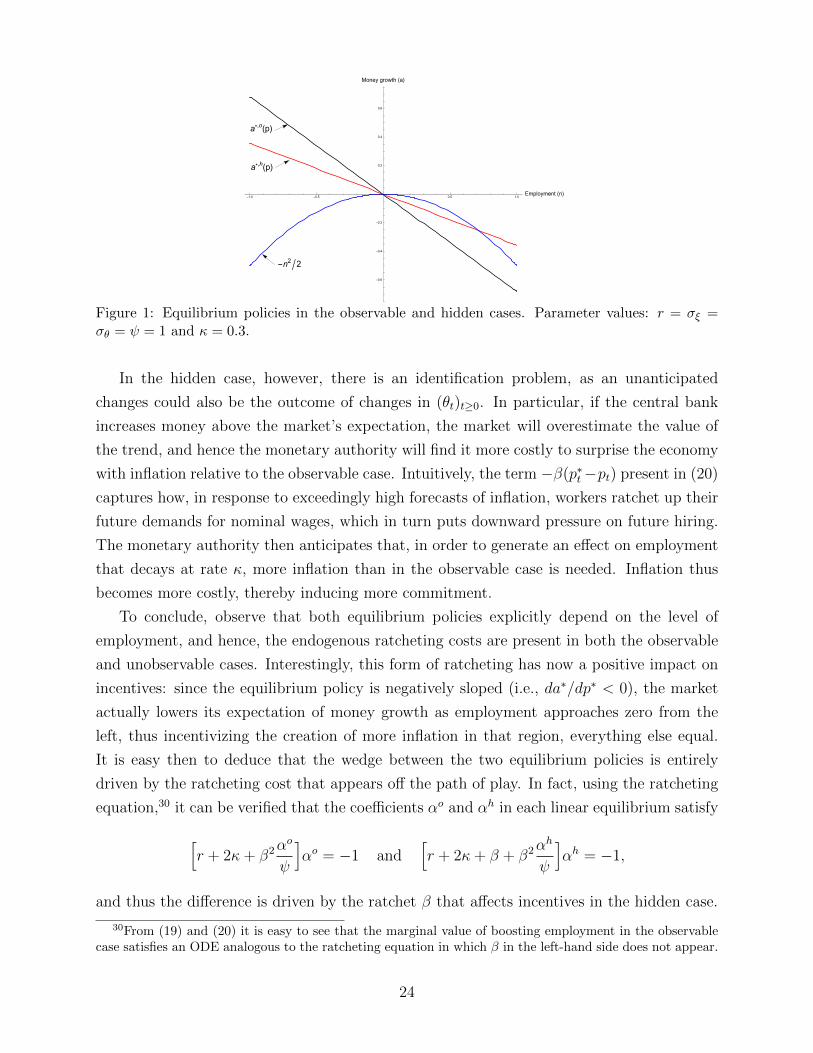
Figure 1: Equilibrium policies in the observable and hidden cases. Parameter values: r = σξ =σθ = ψ = 1 and κ = 0.3.

In the hidden case, however, there is an identification problem, as an unanticipated

changes could also be the outcome of changes in (θt)t≥0. In particular, if the central bank

increases money above the market’s expectation, the market will overestimate the value of

the trend, and hence the monetary authority will find it more costly to surprise the economy

with inflation relative to the observable case. Intuitively, the term −β(p∗t−pt) present in (20)

captures how, in response to exceedingly high forecasts of inflation, workers ratchet up their

future demands for nominal wages, which in turn puts downward pressure on future hiring.

The monetary authority then anticipates that, in order to generate an effect on employment

that decays at rate κ, more inflation than in the observable case is needed. Inflation thus

becomes more costly, thereby inducing more commitment.

To conclude, observe that both equilibrium policies explicitly depend on the level of

employment, and hence, the endogenous ratcheting costs are present in both the observable

and unobservable cases. Interestingly, this form of ratcheting has now a positive impact on

incentives: since the equilibrium policy is negatively sloped (i.e., da∗/dp∗ < 0), the market

actually lowers its expectation of money growth as employment approaches zero from the

left, thus incentivizing the creation of more inflation in that region, everything else equal.

It is easy then to deduce that the wedge between the two equilibrium policies is entirely

driven by the ratcheting cost that appears off the path of play. In fact, using the ratcheting

equation,30 it can be verified that the coefficients αo and αh in each linear equilibrium satisfy

[r + 2κ+ β2α

o

ψ

]αo = −1 and

[r + 2κ+ β + β2α

h

ψ

]αh = −1,

and thus the difference is driven by the ratchet β that affects incentives in the hidden case.

30From (19) and (20) it is easy to see that the marginal value of boosting employment in the observablecase satisfies an ODE analogous to the ratcheting equation in which β in the left-hand side does not appear.

24

4.3 Ratcheting and Thresholds in Earnings Management

This application examines managers’ incentives to boost firms’ earnings reports when they

face strong myopic incentives to exceed a zero-earnings threshold. The main finding is that

firms that are expected to exceed the threshold can actually inflate financial statements

more aggressively than those firms expected to underperform, despite their managers having

weaker myopic incentives. Central to this result is the endogenous ratchet βda∗/dp∗.

A firm’s (cumulative) earnings report process (ξt)t≥0 is given by dξt = (at+θt)dt+σξdZξt .

In this specification, at denotes the degree of earnings manipulation exerted by the firm at

time t ≥ 0, and (θt)t≥0 the firm’s unobserved fundamentals. The latter are assumed to evolve

according to a Brownian martingale dθt = σθdZθt .

I assume that the firm pays its dividends far in the future and that its earnings manage-

ment practices are based on accounting techniques exclusively (e.g., discretionary accruals,

typically difficult to observe). In this case, boosting financial statements imposes no real

costs to the firm in the short- or medium-run, enabling the analysis to isolate learning-

driven ratchet effects. The market then tries to undo the manager’s actions when assessing

short-term performance. Specifically, the market expects the firm’s “natural” earnings over

[t, t+ dt) to take the value Ea∗ [dξt − a∗tdt|Ft] = Ea∗ [θt|Ft]dt = p∗tdt.

The manager is risk neutral and affecting earnings entails private costs captured by ψa2t/2,

ψ > 0. In addition, he is rewarded according to a wage process (χ(p∗t ))t≥0 with χ(·) strictly

increasing, and thus managers who run firms that are perceived to have better fundamentals

receive higher wages.31 Observe that χ′ > 0 implies that the manager always has a myopic

incentive to inflate earnings.

The model represents a situation in which a manager, in any period [t, t+dt), can influence

an accounting division using only the information that he has up to time t; i.e., before the

financial information over [t, t+ dt), dYt = θtdt+ σξdZξt , is processed by such division. This

attempts to capture a firm with a strong internal control system that limits the management’s

direct involvement in the creation of financial statements, but that is not invulnerable to

management pressures. The manager then learns about the firm’s profitability over [t, t+dt)

when a report dξt is produced by the firm’s accounting department (moment at which he

infers dYt = dξt − atdt); but once this occurs, the report cannot be eliminated or modified

before releasing it to the public. Finally, ψa2/2 captures that persuading the accounting

division to inflate earnings by a can be costly at increasing rates (e.g., convex opportunity

cost of resources allocated to this practice, or reluctance to engage in “creative” accounting).

31If (θt)t≥0 represents managerial ability, p∗t is a measure of the manager value: the market expects future

performance to take the form Ea∗[´∞ter(s−t)(dξs − a∗sds)

∣∣∣Ft] = Ea∗[´∞ter(s−t)p∗sds

∣∣∣Ft] = p∗t /r at t ≥ 0.

The independence of χ(·) from a∗ reflects that the market tolerates some degree of earnings management.

25

4.3.1 Linear Benchmark

Suppose that the manager’s flow payoff is linear according to χ(p∗) = αp∗, α > 0. In this

case, the ratcheting equation (14) admits a constant solution given by q(p) = α/(r+β). As a

result, a∗ = (g′)−1(βq(p)) = βα/ψ(r+β), where I used that g′(a) = ψa. Because actions are

constant in this equilibrium, the endogenous ratchet βda∗/dp∗ has no effect on incentives.

Given any nonlinear χ(·), it is then natural to define its linear benchmark policy as

p 7→ βχ′(p)

ψ(r + β).

In fact, if the market’s belief is p, βχ′(p)/ψ(r+β) captures the incentives that would arise in a

linear environment of constant myopic incentives given by α = χ′(p), p ∈ R. As I show next,

this policy is a useful benchmark for illustrating the non-trivial effect that the endogenous

ratchet βda∗/dp∗ can have on incentives in settings where nonlinearities are present.

To conclude this subsection, observe that, in this linear case: (i) as the strength of the

manager’s myopic incentives α increases, earnings are inflated more aggressively; and (ii)

managers of different firms should exert the same degree of manipulation regardless of the

performance of the individual firms they operate.32

4.3.2 Nonlinear Flow Payoffs: The Importance of Thresholds

There is a large body of evidence contradicting that earnings management is uniform across

different levels of performance. In particular, it has been documented that manipulation is

particularly strong around some key thresholds or benchmarks : managers try to avoid (i)

reporting losses, (ii) reporting negative earnings growth, and (iii) failing to meet analyst

forecasts.33 To capture such incentives, I consider a single-peaked marginal utility function:

Assumption 2. χ ∈ C3(R). χ′ is strictly positive, symmetric around zero, and strictly

increasing in (−∞, 0), with χ′(p)→ 0 as p→ −∞. Also, χ′′′(0) < 0.

As in the linear case, the manager has a myopic incentive to boost reported earnings

across all levels of performance (χ′ > 0). However, this incentive is now stronger when

the market expects the firm to generate zero true earnings over the next period (i.e., when

p∗t = 0). I refer to this level of earnings as the zero-earnings threshold.34

32See Stein (1989) for another linear model of earnings management in which equilibrium behavior isindependent of performance but where manipulating earnings entail real costs to the firm.

33See Burgstahler and Dichev (1997), Degeorge et al. (1999), and Dichev et al. (2013) for statistical andsurvey-based approaches to identify this type of practice.

34The symmetry assumption is to illustrate distortions more clearly, whereas the strict concavity of χ′ at

26

Observe that, by positively influencing the market’s belief, a manager standing at p∗ < 0

would face stronger myopic incentives compared to a manager standing at the corresponding

symmetric point |p∗| > 0, thus suggesting that the incentives to inflate earnings should be

stronger to the left of zero. However, recall that managers cannot succeed at misleading the

market in equilibrium. In addition, when κ = 0, beliefs evolve as a martingale along the

path of play, and hence, they are unpredictable. Since the manager’s myopic incentives are

strongest at p∗ = 0, the equilibrium behavior of the public belief suggests that manipulation

should be maximized at the zero-earnings threshold. No conclusive answer is obtained by

appealing to traditional dynamic programming arguments or looking at primitives.

The next result uses an existence result from Section 6.2 pertaining to bounded solu-

tions to the ratcheting equation. Interestingly, the earnings management policy in any such

equilibrium has a different structure from the previously ones just discussed.

Proposition 5. In any Markov equilibrium a∗(p) = βq(p)/ψ, with q(·) a bounded solution to

the ratcheting equation:35 (i) q ∈ (0, χ′(0)/(r+ β)) and q(p)→ 0 as p→ ±∞; (ii) q′(0) > 0

and q′′(0) < 0; (iii) q is maximized strictly to the right of zero; and (iv) the manipulation

policy is skewed to the right of zero, i.e., q(p) ≥ q(−p) for all p > 0.

Proof: See the Appendix.

Proposition 5 uncovers two interesting distortions around the threshold. First, incentives

are depressed at zero relative to the corresponding linear benchmark of slope α = χ′(0) (i.e.,

q(0) < χ′(0)/(r + β)). Second, the policy is maximized to the right of zero, despite those

managers’ weaker myopic incentives than those exactly at the threshold, and despite them

being unable to truly affect the value of the firms they operate. See figure 2.

These two distortions are the consequence of the endogenous ratcheting costs imposed

by the market. To see this, observe that since the manager’s myopic incentives become

stronger as p approaches zero from the left, the market will conjecture a strictly increasing

manipulation profile in this region (da∗/dp∗ > 0). Incentives thus fall below the linear

benchmark in a neighborhood to the left of zero, as successfully influencing the market’s

belief leads firms that are likely to fail meeting the threshold to face a more demanding

incentive scheme. Now, suppose that the market’s conjecture is actually maximized at

zero. In this case, anticipating that the market would revise its conjecture of manipulation

downwards to the right of zero, the manager would be incentivized to boost earnings at the

zero stresses that the myopic incentive at the threshold is acute. This type of marginal incentives can bemicrofounded through a smooth S-shaped contract whose slope is maximized at p∗ = 0.

35An equilibrium of this sort will exist if χ′(0) < ψ√

2rσ2ξ (rσξ + σθ)

2/4σ2θ . See Theorem 3.

27

(p)/ (r + )

a* (p)

Globalmaximum

-2 -1 1 2p

0.1

0.2

0.3

0.4

0.5

a*(p), (p)/ (r+ )

Figure 2: Left panel: the equilibrium policy a∗(·) and the linear benchmark βχ′(p)/ψ(r + β)around zero. Right panel: equilibrium policy degree of skewness to the right, as measured byp 7→ a∗(p) − a∗(−p). a∗(·) is constructed via a solution q(·) to the ratcheting equation on thetruncated domain [−10, 10] with parameter values: r = σξ = σθ = ψ = 1 and χ′(p∗) = e−0.5p∗2 .

zero-earnings threshold. The market must therefore ratchet up its expectation of behavior

at zero (q′(0) > 0) to assess the firm’s fundamentals correctly, resulting in a policy that is

maximized to the right of zero.

Furthermore, the consequences of this endogenous ratcheting extend throughout the en-

tire belief space, yielding a manipulation profile that is skewed to the right of the threshold,

i.e., q(p) > q(−p), p > 0. In fact, observe that in the absence of βda∗/dp∗ = β2q′(p)/ψ on the

left of (14), the ratcheting equation becomes (r+β)q(p) = χ′(p)+σ2q′′(p)/2. By the symme-

try of χ′, however, this ODE admits a symmetric solution around zero: cost smoothing (q′′)

and the ratchet β thus only affect the level of the incentives created, not their skewness. The

ratchet effect discovered is thus more subtle than in the previous applications: the incentives

to maintain high earnings are, on average, stronger than the incentives to build them up.36

5 Equilibrium Analysis: Sufficient Conditions

This section establishes conditions that validate the use of the ratcheting equation for finding

Markov equilibria. More precisely, I present a verification theorem that involves the system

of ODEs (14)–(15): if there is a pair (q, U) that solves the previous system and satisfies a

particular second-order condition, then ρ(βq(·)) is a Markov equilibrium.

Before stating the theorem, it is instructive to illustrate the importance of the first-order

36The following additional properties depicted in the left panel of figure 1 are established in the proofof Proposition 5: q is strictly decreasing to the right of the global maximum; at the global maximum, q isbelow its linear counterpart; there exists a point to the right of the maximum where q changes from beingconcave to convex; and, finally, if q is convex and decreasing, q is above its linear counterpart.

28

approach relative to traditional dynamic programming methods. To this end, observe first

that if the market conjectures a Markov strategy a∗(·), the public and private beliefs follow

dp∗t = [−κ(p∗t − η) + β(pt − p∗t ) + β(at − a∗(p∗t ))]dt+ σdZt, and

dpt = −κ(pt − η)dt+ σdZt,

respectively. Thus, both states are Markov, and (p∗t )t≥0 is controlled by the long-run player.37

It follows that given any private history (ξt, at), the current value of the pair (pt, p∗t ) contains

all the information that is relevant for future decision making. In other words, the long-run

player’s best-response problem to a∗(·) becomes a standard stochastic control problem.

A simple modification of this best-response problem makes dynamic programming meth-

ods also applicable to the equilibrium problem. More precisely, if V (p, p∗) solves

rV (p, p∗) = supa∈A

u(χ(p∗, a∗(p∗)))− g(a)− κ(p− η)Vp(p, p

∗) +σ2

2Vpp(p, p

∗) + σ2Vpp∗(p, p∗)

+[−κ(p∗ − η) + β(p− p∗) + β(a− a∗(p∗))]Vp∗(p, p∗) +σ2

2Vp∗p∗(p, p

∗)

(21)

s.t. arg maxa∈AaβVp∗(p, p)− g(a) = a∗(p) (22)

(subject to transversality conditions), then V (p, p∗) is the long-run player’s value function,

and a∗(p) = ρ(βVp∗(p, p)) is a Markov equilibrium. In fact, constraining the HJB equation

(21) to (22) ensures that the market anticipates the long-run player’s behavior when beliefs

are aligned. Notice, however, that solving (21)–(22) leads to perfect knowledge of (p, p∗) 7→ρ(βVp∗(p, p

∗)), the long-run player’s optimal strategy on and off the equilibrium path. In

other words, the HJB approach, through the exact computation of off-equilibrium payoffs,

implicitly requires the full specification of an MPE to determine on-path behavior.

The key difficulty with (21)–(22) is that it does not correspond to a standard PDE, as

V (p, p∗) depends on Vp∗(p∗, p∗): that is, this differential equation has a non-local structure,

in the sense that it involves the unknown and one of its derivatives each evaluated at different

points. This is because the full-support monitoring technology leads the market to believe

that the long-run player is always on-path taking actions according to ρ(βVp∗(p∗, p∗)). If

a deviation occurs, however, he can also condition his actions on his private belief, and

ρ(βVp∗(p, p∗)) and ρ(βVp∗(p

∗, p∗)) need not coincide; in those cases, incentives for double

deviations (i.e., deviations after deviations) appear. To the best of my knowledge, no general

existence theory for this type of equation is available.38

37From Lemma 1, the dynamic for (p∗t )t≥0 follows directly from dp∗t = −κ(p∗t − η)dt+βσξ[dξt− (a∗(p∗t ) +p∗t )dt] and dξt = (at + pt)dt+ σξdZt from the long-run player’s perspective.

38In the linear case, there is solution to (21)–(22) that is additively separable in p and p∗, so the non-

29

The technical importance of the ratcheting equation thus lies on opening a venue to find

Markov equilibria bypassing all these difficulties. In fact, as a self-contained object, this

equation suggests that computing off-path payoffs exactly is by no means strictly necessary

to determine equilibrium behavior. This is confirmed in the next subsection.

Remark 6 (The ratcheting equation as a necessary condition for MPE). Applying the

envelope theorem to (21)–(22) yields that q(p) := Vp∗(p, p), which characterizes on-path

incentives via (22), satisfies the ratcheting equation (14). Thus, the ratcheting equation is a

necessary condition for MPE when the value function is sufficiently differentiable. The ODE

for U(p) := V (p, p) then follows from evaluating (21)–(22) at p = p∗.

5.1 A Verification Theorem for Markov Equilibria

As before, let a∗(p) := ρ(βq(p)) with q(·) a solution to the ratcheting equation. Off the path

of play, the long-run player can condition his actions on both (Zt)t≥0 (which drives (pt)t≥0)

and (∆t)t≥0; denote by F(Z,∆) := (FZ,∆t )t≥0 the corresponding filtration. In this context,

a strategy (at)t≥0 is said to be admissible if (i) it is F(Z,∆)-progressively measurable; (ii)

E[´ t

0(as)

2ds]< ∞, t ≥ 0; and (iii) E

[´∞0e−rt|u(χ(pt + ∆∗t , a

∗(pt + ∆∗t )))− g(at)|dt]< ∞,

where (∆∗t )t≥0 denotes the solution to (8) under the pair (a∗(·), (at)t≥0).39

Theorem 1 (Verification Theorem). Suppose that (q, U) of class C2(R) solves (14)–(15)

and that a∗(·) := ρ(βq(·)) is interior. Moreover, assume that

(i) There exist C1, C2, and C3 > 0 such that |U(p)| ≤ C1(1 + |p|2) (quadratic growth),

|U ′(p)| ≤ C2(1 + |p|) (linear growth), and |q(p1)− q(p2)| ≤ C3|p1 − p2| (Lipschitz);

(ii) limt→∞

E[e−rtU(pt + ∆∗t )] = limt→∞

E[e−rtq(pt + ∆∗t )(∆∗t )] = lim

t→∞E[e−rtU ′(pt + ∆∗t )(∆

∗t )] = 0

for all (at)t≥0 admissible, where (pt, ∆∗t )t≥0 is the solution to (5)–(8) under (a∗(·), (at)t≥0);

(iii) U ′′ and q′ satisfy

|U ′′(p)− q′(p)| ≤ ψ(r + 4β + 2κ)

4β2, for all p ∈ R. (23)

Then, if (ρ(βq(p∗t )))t≥0 is feasible, a∗(·) = ρ(βq(·)) is a Markov equilibrium.

localness disappears: Vp∗(p∗, p∗) becomes a constant, and is thus independent of (p∗, p∗). The economicimplication is that the long-run player finds it optimal to take the same action on and off the path of play.Observe also that the technical complexities just described are present in any setting involving two-sidedlearning and imperfect monitoring in which one belief can be actively controlled.

39This is the direct extension of admissibility from Section 2 to strategies that can condition actions oninformation off the path of play.

30

Proof : See the Appendix.

Theorem 1 offers a method for finding Markov equilibria that relies on solving a system

of equations for (q, U), in the same way that traditional verification theorems in dynamic

programming offer a way to find optimal policies by solving HJB equations. The advantages

of this theorem are clear: first, it bypasses all the difficulties encountered in attempting to find

equilibria by computing off-path payoffs exactly; second, it is general, with weak restrictions

on payoffs; and third, by involving a system of ODEs, the derivation of qualitative properties

of equilibrium behavior becomes considerably simpler.

Regarding the assumptions in the Theorem, the Lipschitz condition on q(·) ensures that

a solution to (p∗t )t≥0 (and, hence, to (∆)t≥0) exists and is unique under (i) and (ii) of the

admissibility concept, and thus, the long-run player’s best-response problem is well defined.

The conditions on U in turn guarantee that the U -ODE (15) has as a unique solution

U(p) := E[ˆ ∞

0

e−rt[u(χ(pt, ρ(βq(pt))))− g(ρ(βq(pt)))]dt∣∣∣ p0 = p

],

i.e., the payoff from following the market’s conjecture a∗(·) = ρ(βq(·)). The rest of the

assumptions are used to construct an upper bound for the long-run player’s value function,

with the property that it coincides with U(·) on the equilibrium path; but since U(·) can

be achieved by following a∗(·) when beliefs are aligned, it follows that inducing no belief

asymmetry is optimal. Finally, the feasibility requirement demands that (2) has a unique

solution under a∗(·) to ensure that the outcome of the game is well and uniquely defined.

This requirement is verified in the two classes of games studied in Section 6.

Condition (23) has an economic interpretation: it is a bound on the rate of change of

U ′(p)−q(p), and the latter is an information rent ; i.e., a measure of the value of having private

information about the fundamentals. To see why, recall that both U ′ and q incorporate

the costs of matching the changes in the market’s conjecture of equilibrium behavior. In

addition, q(p) incorporates the cost of adjusting behavior to explicitly account for belief

asymmetry; this is absent in U ′(p) because beliefs are aligned along the path of play. The

difference q(p) − U ′(p) is thus a measure of the value of having private information about

the fundamentals in the form of a (marginally) more pessimistic private belief; U ′(p)− q(p)is then the analog measure for the case of a (marginally) more optimistic private belief.

Rates of change of information rents appear when approximating the payoff of an al-

ternative strategy using information rents to estimate the continuation value following a

partial deviation from a∗(·). This estimation procedure is appropriate because the long-run

player has private information off the path of play, and hence, estimating the payoff of an

31

alternative strategy requires accounting for the value of such private information; but the

only information available in this procedure is the one conveyed by (q, U) solving (14)–(15).

Moreover, as the long-run player’s private belief changes, his continuation payoff varies, and

so the payoff of an alternative strategy necessarily depends on U ′′ − q′. When (23) holds, it

can be ensured that it is never optimal for the long-run player to induce any degree of belief

asymmetry, and thus U ′′ − q′ can be seen as a global measure of the value of such private

information. The presence of an absolute value simply reflects the possibility of upward or

downward deviations being profitable depending on how the market rewards the long-run

player. Finally, (23) can be relaxed, depending on the primitives of the environment at hand;

this is the case in the class of linear-quadratic games presented in the next section.

Remark 7 (On the first-order approach in optimal contracting). Similar sufficient conditions

have also appeared in the optimal contracting literature, with the corresponding measures

of information rents in the form of stochastic processes rather than ODEs, due to the non-

Markov nature of such environments. In particular, this paper has built on Williams (2011)

and Sannikov (2014) who find sufficient conditions that validate their first-order approaches

via using measures of information rents in quadratic bounds for payoffs after deviations.40

By recognizing that a full specification of the long-run player’s best response is only suffi-

cient for the analysis of equilibrium outcomes, this paper shows that the methods from the

optimal contracting literature are applicable to games of learning and unobserved actions.

Importantly, Section 6 goes a step further relative to this literature by showing that (23)

can be mapped to primitives for a wide range of settings.

6 Existence of Markov Equilibria

This section uses Theorem 1 to derive two existence results for Markov equilibria that can

be computed using the ratcheting equation. This is conducted by (i) proving the existence

of solutions to the system (14)–(15) and (ii) verifying that the second-order condition (23)

holds. The advantage of the verification theorem is that, by involving ODEs, (23) can be

verified on primitives in many economic environments. (It can always be verified ex post.)

The environments under study are (i) linear quadratic games and (ii) games with bounded

marginal flow payoffs. In the former, equilibrium behavior is linear in the public belief. In the

latter, equilibria are fully nonlinear. As argued earlier, to focus on the question of existence

40Their second-order conditions are one-sided only. This is because Williams (2011) allows for downwarddeviations only, and in Sannikov (2014) actions do not affect the public signal directly. My construction isclosest to Sannikov’s (2014).

32

of equilibria when the ratchet principle appears in its most traditional form, the next two

sections restrict the analysis to the case in which the market’s action χ is independent of a∗.

6.1 Linear Quadratic Games

Definition 4. The environment is said to be linear quadratic if A = R; g(a) = ψ2a2, ψ > 0;

and h(p∗) := u(χ(p∗, a∗)) = u0 + u1p∗ − u2p

∗2t , where u0, u1 ∈ R and u2 ≥ 0.

The next result shows the existence of a linear Markov equilibrium.

Theorem 2. Consider a linear quadratic environment. A linear q(·) and a quadratic U(·)solving (14) and (15), respectively, exist if and only if

u2 ≤ψ(r + β + 2κ)2

8β2. (24)

In this case, a∗(p) = β[q1 + q2p]/ψ, with

q1 =ηκq2 + u1

r + β + κ+ β2

ψq2

and q2 =ψ

2β2

[−(r + β + 2κ) +

√(r + β + 2κ)2 − 8u2β2

ψ

]< 0,

is a linear Markov equilibrium.

Proof: See the Appendix.

The linear equilibrium found entails a negative slope q2 and an intercept q1 that can take

any sign. Suppose that u1 = 0, so flow payoffs are maximized at zero. In this case, for large

|p|, the long-run player has a myopic incentive to drive the public belief towards the bliss

point, and thus, q2 < 0. Interestingly, when η > 0, q1 is negative, so the long-run player puts

downward pressure on the public belief at the bliss point. The reason is cost smoothing: if

p∗ = 0, the long-run player expects the public belief to revert to η > 0 with high probability,

but when p∗ ∈ [0, η], driving p∗ back to zero is optimal. Because the disutility of effort is

convex, it is optimal to set a∗(0) < 0 to distribute such costs optimally over time.

The curvature condition (24) corresponds to a necessary and sufficient condition for a

linear solution to the ratcheting equation (14) to exist in the first place; thus, its violation

is not an indication that a linear equilibrium ceases to exist due to the value of acquiring

private information about the fundamentals becoming too large.41 Instead, the existence

41Recall that verification theorem requires a solution (q, U) to the system (14)–(15) to exist to make thesecond-order condition (23) applicable. For linear quadratic games, however, the curvature condition (24)is the relevant constraint, as when this one is satisfied, a relaxed version of (23) tailored for this particularclass of games can be verified to hold.

33

problem operates through the endogenous ratcheting channel.

To see this, notice that as u2 grows, the myopic incentive to drive the public belief

towards the bliss point increases in absolute value. Thus, in a linear equilibrium, the market

must impose a steeper conjecture a∗(·) to control such incentives. A steeper conjecture,

however, also makes the market revise its expectation of performance more drastically given

any changes in beliefs. Consequently, an upward (downward) deviation to the left (right)

of zero becomes more attractive, as it now leads to a more rapid decrease in the market’s

expectation of performance tomorrow; in the ratcheting equation, this is captured by the

left-hand side r + κ + β + βda∗/dp∗ decreasing as da∗/dp∗ becomes more negative. Thus,

if (24) is violated, a linear conjecture cannot control both (i) myopic incentives and (ii) the

incentives to induce the market to ratchet down its expectations of effort.

Finally, if flow payoffs are linear, the curvature condition is trivially satisfied, and thus,

a linear equilibrium always exists. In this case, u2 = 0 leads to q2 = 0 in Theorem 2, and

hence, to an equilibrium with constant actions defined by

q(p) = q1 =u1

r + β + κ⇒ g′(a∗) = β

u1

r + β + κ.

Moreover, a linear U(·) solves (15) in this case, which yields U ′′ − q′ ≡ 0. Put differently,

changes in the long-run player’s private information have no value for the long-run player,

which is consistent with the equilibrium level of effort found by Holmstrom (1999) being also

optimal off the path of play.

6.2 Bounded Marginal Flow Payoffs

Definition 5. Let h(p) := u(χ(p)). A game is one of bounded marginal flow payoffs if

(i) (Boundedness) ∃ m,M ∈ R s.t. −∞ < m := infp∈R

h′(p) ≤ supp∈R

h′(p) := M <∞, and

(ii) (Interior actions) A is compact and βx | x ∈ [m/(r+β+κ),M/(r+β+κ)] ⊆ g′(A).

I now show that there exists a solution (q, U) to (14)–(15). A solution to (14) satisfying

that both q and q′ are bounded will be referred to as a bounded solution—the focus will be

on this type of solution.42

42Searching for a bounded q is natural given that marginal flow payoffs are bounded. A bounded q′ inturn ensures that a∗(p) := ρ(βq(p)) is Lipschitz and that U ′ satisfies the transversality and growth conditionsof Theorem 1.

34

Proposition 6 (Existence of Bounded Solutions to the Ratcheting Equation).

There exists q ∈ C2(R), a bounded solution to the ratcheting equation, such that

q(p) ∈[

m

r + β + κ,

M

r + β + κ

], for all p ∈ R. (25)

If, in addition, h′+ := limp→∞

(u χ)′(p) and h′− := limp→−∞

(u χ)′(p) exist, any bounded solution

satisfying (25) also verifies that

limp→+∞

q(p) =h′+

r + β + κand lim

p→−∞q(p) =

h′−r + β + κ

. (26)

Proof: See the Appendix.

Bound (25) states that there is a candidate equilibrium that lies in between the equilibria

that would arise in environments of linear flow payoffs with slopes m and M . The second

part of the proposition in turn asserts that, in settings where marginal flow payoffs become

asymptotically constant (as in the earnings management application of Section 4.3), equilib-

rium behavior converges to the corresponding limit (linear) counterpart (i.e., u(χ(p)) = h′+p

or h′−p) as p → ±∞. While this asymptotic property of payoffs is not required for the ex-

istence results presented below, it provides useful guidance as to which type of “boundary”

conditions to expect when searching for a solution to the second-order ODE (14).

Proposition 7 (Long-Run Player’s Equilibrium Payoff). Let q denote a bounded so-

lution to (14). The unique solution to the ODE (15) is given by

U(p) = E[ˆ ∞

0

e−rt[h(pt)− g(ρ(βq(pt)))]dt∣∣∣ p0 = p

], (27)

where dpt = −κ(pt − η)dt + σdZt for t > 0 and p0 = p. Furthermore, U has linear growth,

and U ′ is bounded.

Proof: See the Appendix.

Finally, I establish conditions on the primitives (r,m,M,ψ, κ, σθ, σξ) that ensure that

(q, U) as above meets the requirements of Theorem 1. I do this for the case κ = 0, which

simplifies the estimation of the rate of change of information case, as I explain shortly.

35

Theorem 3 (Existence of Markov Equilibrium). Suppose that κ = 0, and let q : R→ Rdenote a bounded solution to the ratcheting equation (14). If

M −mψ

≤

√2rσ2

ξ (r + β)2

4β2=

√2rσ2

ξ (rσξ + σθ)2

4σ2θ

, (28)

a∗(·) := ρ(βq(·)) is a Markov equilibrium.

Proof: See the Appendix.

Theorem 3 proves the existence of equilibria in which behavior is a nonlinear function

of the common belief for a wide range of economic environments. Condition (28) is relaxed

when the public signal is noisy (σξ is large) and when the environment is less uncertain (σθ

is small), as in this case, beliefs become less responsive to signal surprises. The condition

is also relaxed when affecting the public signal is costly (ψ is large), the long-run player is

impatient (r is large), and when M −m falls. It is also trivially satisfied when payoffs are

linear (M = m), as information rents are constant in this case (leading to U ′′ − q′ ≡ 0).

The main challenge in the proof of Theorem 3 is the estimation of the rate of change of

information rents in terms of primitives. When κ = 0, the analysis is simplified by the fact

that |U ′′− q′| can be expressed as an analytic function of q, and the bounds for q in terms of

primitives follow from Proposition 6. To the best of my knowledge, no such analytic solution

exists when κ > 0, thus making the estimation more complex.43

Importantly, mean reversion can be only expected to reduce the attractiveness of any

deviation. In fact, as κ increases, beliefs become less sensitive to new information (β(κ) =

(κ2 + σ2θ/σ

2ξ )

1/2 − κ falls with κ), and any shock to beliefs decays faster; a marginal increase

in effort has then a smaller and shorter impact on flow payoffs. Moreover, since belief

asymmetry decays at rate β + κ = (κ2 + σ2θ/σ

2ξ )

1/2, the long-run player’s informational

advantage also disappears faster as κ grows. While higher rates of mean reversion are

likely to reduce the strength of the ratcheting performed by the market (as beliefs become

more i.i.d.), ratcheting appears only to the extent that beliefs are revised in response to new

information, and hence, it is likely to be dominated by the sensitivity effect. This is confirmed

in linear environments where incentives are characterized by βq(p) = β(κ)/(r + β(κ) + κ):

while the exogenous ratchet term β(κ) in the denominator decreases with κ, incentives still

decay due to beliefs becoming less responsive to signal surprises.

43Specifically, U ′′ − q′ satisfies a type of ODE whose solutions are constructed using confluent hypergeo-metric functions, which take the form of power series (cf. Abramowitz and Stegun, 1964).

36

7 Conclusions

This paper has examined a class of continuous-time games of learning and imperfect moni-

toring. The contribution is twofold. First, the analysis executed uncovered a learning-driven

version of the ratchet principle that naturally appears in settings characterized by com-

mon uncertainty and strategic behavior. Second, this paper expanded the class of economic

questions that can be studied under the umbrella of signal jamming models beyond linear

settings. The applications developed are in fact at the intersection of these areas: they

explore ratchet effects in settings that exhibit nonlinearities.

Assuming ex ante symmetric uncertainty is a convenient modeling technique to analyze

incentives in settings where uncertainty is common to everyone. If the long-run player had ex

ante superior information about the fundamentals, for instance, his actions could potentially

incorporate his private information. Beyond linear quadratic games (linear learning, linear

quadratic payoffs) or settings in which the fundamentals take finite values, the long-run

player’s action would then be a nonlinear function of his private information, which makes

handling beliefs technically challenging.44 Relatedly, necessary and sufficient conditions for

Markov equilibria away from stationary learning can be obtained using identical arguments

to the ones employed here. The challenge then becomes to show the existence of solutions

to a version of the ratcheting equation that also depends on time as a state.

Finally, I discuss three possible extensions of the model. First, since in any nonlinear

Markov equilibrium, actions are a nonlinear function of the complete history of signal real-

izations, the class of distributions that can be generated for the public signal is quite rich

(and not necessarily Gaussian). Thus, the model has the potential to be used to address

empirical questions in environments with inherent nonlinearities. Second, pure-strategy equi-

libria beyond the Markov case could be studied as well, the main difference being that the

corresponding necessary and sufficient conditions would involve stochastic processes rather

than ODEs. Since Markov equilibria are already a function of the complete public history

via the public belief, it is unclear whether this extension produces any new insights. Third, a

natural extension involves studying incentives in environments where affecting the informa-

tiveness of the public signal is possible, such as when there are complementarities between

the fundamentals and actions. While the first-order approach followed here is still applicable

in settings beyond the additively separable world, the analysis is complicated by additional

experimentation effects. These and other questions are left for future research.

44See Bonatti, Cisternas and Toikka (2016) for a linear quadratic model of oligopoly with imperfect publicmonitoring in which firms have private information regarding their constant marginal costs.

37

References

[1] Abramowitz, M. and I. Stegun (1964): Handbook of Mathematical Functions, with For-

mulas, Graphs, and Mathematical Tables. New York: Dover.

[2] Atkeson, A., V.V. Chari and P. Kehoe (2007): “On the Optimal Choice of a Monetary

Policy Instrument,” Federal Reserve Bank of Minneapolis Staff Report 394.

[3] Bar-Isaac, H. and J. Deb (2014): “What is a Good Reputation? Career Concerns with

Heterogeneous Audiences,” International Journal of Industrial Organization, 34, 44-50.

[4] Bergemann, D. and U. Hege (2005): “The Financing of Innovation: Learning and Stop-

ping,” RAND Journal of Economics, 36(4), 719-752.

[5] Bhaskar, V. (2014): “The Ratchet Effect Re-Examined: A Learning Perspective,” Work-

ing Paper, UCL.

[6] Bhaskar, V. and G. Mailath (2016): “The Curse of Long Horizons,” Working Paper,

University of Pennsylvania.

[7] Board, S. and M. Meyer-ter-Vehn (2014): “A Reputational Theory of Firm Dynamics,”

Working Paper, UCLA.

[8] Bohren, A. (2016): “Using Persistence to Generate Incentives in a Dynamic Moral

Hazard Problem,” Working Paper, University of Pennsylvania.

[9] Bonatti, A., G. Cisternas and J. Toikka (2016): “Dynamic Oligopoly with Incomplete

Information,” Review of Economic Studies, forthcoming.

[10] Bonatti, A. and J. Horner (2011): “Collaborating,” American Economic Review, 101(2),

632-663.

[11] Bonatti, A., and J. Horner (2016): “Career Concerns with Exponential Learning,”

Theoretical Economics, forthcoming.

[12] Burgstahler, D. and I. Dichev (1997): “Earnings management to avoid earnings de-

creases and losses,” Journal of Accounting and Economics, 24(1), 99-126.

[13] Cogley, T., G. Primiceri and T. Sargent (2010): “Inflation-Gap Persistence in the US,”

American Economic Journal: Macroeconomics, 2(1), 43-69.

[14] Cohen, S. and R. Elliott (2015): Stochastic Calculus and Applications, Second Edition.

New York: Birkhauser.

38

[15] Cukierman, A. and A. Meltzer (1986): “A Theory of Ambiguity, Credibility, and Infla-

tion under Discretion and Asymmetric Information,” Econometrica, 54(5), 1099-1128.

[16] Da Prato, G. and J. Zabczyk (1992): Stochastic Equations in Infinite Dimensions.

Cambridge University Press.

[17] De Coster, C. and P. Habets (2006): Two-Point Boundary Value Problems: Lower

and Upper Solutions. Mathematics in Science and Engineering, Vol. 205 (First Ed.).

Amsterdam: Elsevier.

[18] Degeorge, F., J. Patel and R. Zeckhauser (1999): “Earnings Management to Exceed

Thresholds,” The Journal of Business, 72(1), 1-33.

[19] Dichev, I., J. Graham, H. Campbell and S. Rajgopal (2013): “Earnings Quality: Evi-

dence From the Field,” Journal of Accounting and Economics, 56, 1-56.

[20] Di Nunno, G., B. Oksendal and F. Proske (2009): “Malliavin Calculus for Levy Pro-

cesses with Applications to Finance.” Berlin: Springer-Verlag.

[21] Dixit, A. and R. Pyndick (1994): Investment Under Uncertainty. Princeton: Princeton

University Press.

[22] Faingold, E., and Y. Sannikov (2011): “Reputation in Continuous-Time Games.” Econo-

metrica, 79(3), 773-876.

[23] Gali, J. (2008): Monetary Policy, Inflation, and the Business Cycle. Princeton: Prince-

ton University Press.

[24] Holmstrom, B. (1999): “Managerial Incentive Problems: A Dynamic Perspective,” The

Review of Economic Studies, 66, 169-182.

[25] Horner, J. and L. Samuelson (2014): “Incentives for Experimenting Agents,” RAND

Journal of Economics, 44, 632-663.

[26] Karatzas, I. and S. Shreve (1991): Brownian Motion and Stochastic Calculus. New York:

Springer-Verlag.

[27] Kovrijnykh, A. (2007): “Career Uncertainty and Dynamic Incentives,” Working paper,

University of Chicago.

[28] Kydland, F. and E. Prescott (1977): “Rules Rather Than Discretion: The Inconsistency

of Optimal Plans,” Journal of Political Economy, 85(3), 473-491.

39

[29] Laffont, J.J. and J. Tirole (1988): “The Dynamics of Incentive Contracts,” Economet-

rica, 56(5), 1153-1175.

[30] ——. (1994): A Theory of Incentives in Procurement and Regulation. Cambridge: MIT

Press.

[31] Liptser, R. and A. Shiryaev (1977): Statistics of Random Processes I and II. New York:

Springer-Verlag.

[32] Martinez, L. (2006): “Reputation and Career Concerns,” Mimeo, Federal Reserve Bank

of Richmond.

[33] Martinez, L. (2009): “Reputation, Career Concerns, and Job Assignments,” The B.E.

Journal of Theoretical Economics, Berkeley Electronic Press, 9(1, Contributions), Ar-

ticle 15.

[34] Meyer, M. and J. Vickers (1997): “Performance Comparisons and Dynamic Incentives.”

Journal of Political Economy, 105(3), 547-581.

[35] Pham, H. (2009): Continuous-time Stochastic Control and Optimization with Financial

Applications. Berlin: Springer.

[36] Prat, J. and B. Jovanovic (2014): “Dynamic Contracts when the Agent’s Quality is

Unknown,” Theoretical Economics, 9(3), 865-914.

[37] Rogers, L. C. G. and D. Williams (1987): Diffusions, Markov Processes and Martingales.

Vol. 2. Ito Calculus. New York, Wiley.

[38] Sannikov, Y. (2007): “Games with Imperfectly Observable Actions in Continuous

Time,” Econometrica, 75(5), 1285-1329.

[39] Sannikov, Y. (2014): “Moral Hazard and Long-Run Incentives,” Working paper, Prince-

ton University.

[40] Stein, J. (1989): “Efficient Capital Markets, Inefficient Firms: A Model of Myopic

Corporate Behavior,” Quarterly Journal of Economics, 104, 655-669.

[41] Stock, J. and M. Watson (2007): “Why Has U.S. Inflation Become Harder to Forecast?,”

Journal of Money, Credit and Banking, 39, 3-33.

[42] Williams, N. (2011): “Persistent Private Information,” Econometrica, 79(4), 1233-1275.

40

Appendix

Throughout this Appendix:

• Instead of looking at the system (p, p∗), I work with (p,∆) where ∆ := p∗ − p evolves

according to d∆t = [−(β + κ)∆t + β(at − a∗t )]dt (eqn. (8)). This avoids carrying the

same Brownian motion twice in the off-path analysis.

• Since, p∗t = pt along the path of play, and dpt = −κ(pt − η)dt + σdZt, it follows that

pt ∼ N (po, σ2t) when κ = 0, and pt ∼ N (e−κtpo + (1 − eκtη), σ2(1 − e−2κt)/2κ) when

κ > 0, from a time-zero perspective. In either case, limt→∞

E[e−rtpt] = limt→∞

E[e−rtp2t ] = 0.

Proof of Proposition 1. Consider the strategy aεt = a∗t + ∆t + λεt, t ≥ 0, where: (i) a∗t

denotes the market’s current conjecture of equilibrium play at time t ≥ 0; (ii) ∆t denotes

the current degree of belief asymmetry at time t ≥ 0; and where (iii) (εt)t≥0 is (FZ,∆t )t≥0-

progressively measurable and satisfies εt < ε, a.s. for all t ≥ 0, some ε > 0.

It is easy to see that the induced process of belief asymmetry, (∆εt)t≥0, is given by

∆εt = ∆ε

t(λ) := λβ

ˆ t

0

e−κ(t−s)εsds, t ≥ 0,

and that the latter grows at most linearly in time (for κ > 0 it is even bounded). Also,

p∗t = pt + ∆εt(λ), where dpt = −κ(pt − η)dt+ σdZt, t ≥ 0.

The payoff of following (aεt)t≥0 is given by

V ε(λ) = E

[ˆ ∞0

e−rt[u(χ(pt+∆εt(λ), a∗(pt + ∆ε

t(λ)))︸ ︷︷ ︸a∗t=

)−g(a∗(pt + ∆εt(λ)) + ∆ε

t(λ) + λεt︸ ︷︷ ︸aεt :=

)]dt

].

Let `(p) = u(χ(p, a∗(p))) − g(a∗(p)). Since a∗(·) is Lipschitz, the differentiability and

growth conditions in Assumption 1 ensure that `(·) is differentiable and that `(·) and `′(·)have polynomial growth. Thus, letting L(ω, t, λ) := u(χ(pt + ∆ε

t(λ), a∗(pt + ∆εt(λ)))) −

g(a∗(pt + ∆εt(λ)) + ∆ε

t(λ) + λεt), there are C > 0 and j ∈ N such that, if λ ∈ (−δ, δ), δ > 0,∣∣∣∂L∂λ

∣∣∣ ≤ Ct(1 + |pt + t|j),

as (∆εt)t≥0 grows at most linearly in time. Since (pt)t≥0 is Gaussian—with a mean process

that is bounded and a variance that grows at most linearly in time—the function e−rtCt(1 +

|pt + t|j) is integrable with respect to dP × dt, where P is the measure under which (Zt)t≥0

41

(defined in Lemma 1) is a Brownian motion, and dt is the Lebesgue measure; a similar

argument shows that (ω, t) 7→ e−rtL(ω, t, λ) is also integrable for all λ ∈ (−δ, δ). Since

e−rtCt(1 + |pt + t|j) does not depend on λ, it follows that V ε(λ) is differentiable over (−δ, δ).Letting f(p) = u(χ(p, a∗(p))), it is easy to see that

dV ε

dλ

∣∣∣λ=0

= E[ˆ ∞

0

e−rt(f ′(pt)− g′(a∗(pt))

[da∗dp∗

(pt) + 1])(

β

ˆ t

0

e−κ(t−s)εsds

)− g′(a∗(pt))εt

dt

]= E

[ˆ ∞0

e−rtεt

β

ˆ ∞t

e−(r+κ)(s−t)(f ′(ps)− g′(a∗(ps))

[da∗dp∗

(ps) + 1])ds− g′(a∗(pt))

dt

],

where the last equality follows from integration by parts. Also, observe that

q(p) := E[ˆ ∞

t

e−(r+κ)(s−t)(f ′(ps)− g′(a∗(ps))

[da∗

dp∗(ps) + 1

])dt∣∣∣pt = p

],

is finite, consequence both of the growth conditions in Assumption 1 and of a∗(·) being Lip-

schitz. It follows that in an interior equilibrium g′(a∗(pt)) = βq(pt) must hold a.s. at all

times; otherwise the long-run player can choose εt such that εt[βq(pt) − g′(a∗t )] > 0, t ≥ 0,

thus increasing his payoff.

Proof of Proposition 2: Let f(p) = u(χ(p, a∗(p))) and recall that dpt = −κ(pt−η)dt+σdZt,

t ≥ 0. From the proof of the Proposition 1, the random variable

X :=

ˆ ∞0

e−(r+κ)t

(f ′(pt)− g′(a∗(pt))

[da∗

dp∗(pt) + 1

])dt

is integrable. It follows that Yt := E[X|Ft], t ≥ 0, is a martingale; in particular, a local mar-

tingale. By the Martingale Representation Theorem (Theorem 36.5 in Rogers and Williams,

1987), there exists a predictable process (Ht)t≥0 such that Yt =´ t

0HsdZs a.s., t ≥ 0.

On the other hand, observe that

Yt =

ˆ t

0

e−(r+κ)s

(f ′(ps)− g′(a∗(ps))

[da∗

dp∗(ps) + 1

])ds+ e−(r+κ)tq(pt).

Since q(·) is of class C2 (consequence of g′(a∗(p)) = βq(p) and of a∗ and ρ := (g′)−1 being

of class C2), Ito’s rule yields that the drift of the Ito process on the right-hand side of the

42

previous expression must satisfy

0 = f ′(pt)− g′(a∗(pt))[da∗

dp∗(pt) + 1

]− (r + κ)q(pt)− κ(pt − η)q′(pt) +

1

2σ2q′′(pt),

as Yt =´ t

0HsdZs, a.s., t ≥ 0. Using that a∗(p) = ρ(βq(p)) it then follows that

[r + κ+ β + β2ρ′(βq(p))q′(p)

]q(p) =

d

dp[u(χ(p, ρ(βq(p))))]

∣∣∣p=pt− κ(p− η)q(p) +

1

2σ2q′′(p).

Regarding U(p) = E[´∞

0e−rt[u(χ(pt, a

∗(pt)))− g(a∗(pt))]dt∣∣∣p0 = p

], this function is of

class C2 by definition of a Markov equilibrium. Also, by the growth conditions in Assumption

1 and a∗(·) being Lipschitz, the random variable X :=´∞

0e−rt[u(χ(pt, a

∗(pt)))− g(a∗(pt))]dt

is integrable. Following the same steps taken to derive the q-ODE (namely, constructing the

martingale Yt = E[X|Ft], and then using Ito’s rule) yields that

rU(p) = u(χ(p, ρ(βq(p))))− g(ρ(βq(p)))− κ(p− η)U ′(p) +1

2σ2U ′′(p).

Proof of Theorem 1: Suppose the market constructs beliefs using a∗(·) := ρ(βq(·)), with

q(·) as in the theorem. Off the path of play, the private and the public belief are given by

dp∗t = [−κ(p∗t − η) + β(pt − p∗t ) + β(at − a∗(p∗t ))]dt+ σdZt, where

dpt = −κ(pt − η)dt+ σdZt.

Notice that |(a∗)′(p)| = |βq′(p)|/g′′(a∗(p)) ≤ βC/ψ, where C is the Lipschitz constant of

q(·). Thus, the previous system has a drift and volatility that are globally Lipschitz, which

guarantees that it admits a strong solution for any strategy that satisfies (i) and (ii) in the

admissibility concept of Section 5.2 (Theorem 1.3.15 in Pham 2009). The long-run player’s

optimization problem is thus well-defined over the set of admissible strategies.

Take any solution (q, U) as in the theorem. Consider the function

U(p+ ∆) + [q(p+ ∆)− U ′(p+ ∆)]∆ +Γ

2∆2. (A.1)

I will show that, for a suitably chosen Γ, the assumptions in the theorem ensure that this

function is an upper bound to the long-run player’s payoff under any feasible strategy.

43

More concretely, given a feasible strategy a := (at)t≥0, define the process

Vt :=

ˆ t

0

e−rs[h(ps+∆t)−g(as)]ds+e−rtU(pt + ∆t) + [q(pt + ∆t)− U ′(pt + ∆t)]∆t +

Γ

2∆2t

,

where h(p) := (u χ)(p, a∗(p)), and ∆ denotes the belief asymmetry process under the pair

(a∗(p∗t ), a). Applying Ito’s rule to V ,

dVte−rt

= [h(p∗t )− g(at)]dt− rU(p∗t ) + [q(p∗t )− U ′(p∗t )]∆t +

Γ

2∆2t

dt

+

U ′(p∗t )[−κ(p∗t − η)− β∆t + β(at − a∗(p∗t ))] +

1

2σ2U ′′(p∗t )

︸ ︷︷ ︸

(A)

dt

+∆t

q′(p∗t )[−κ(p∗t − η)− β∆t + β(at − a∗(p∗t ))] +

1

2σ2q′′(p∗t )

︸ ︷︷ ︸

(B)

dt

−∆t

U ′′(p∗t )[−κ(p∗t − η)− β∆t + β(at − a∗(p∗t ))] +

1

2σ2U ′′′(p∗t )

︸ ︷︷ ︸

(C)

dt

+[q(p∗t )− U ′(p∗t )][−(β + κ)∆t + β(at − a∗(p∗t ))]dt

+Γ∆t[−(β + κ)∆t + β(at − a∗(p∗t ))]dt+ Brownian term,

where I have used that p∗t := pt+∆t evolves according to dp∗t = (−κ(p∗t −η)+β(a−a∗(p∗t ))−β∆t)dt+ σdZt. Now, using (15) and (14) yields

(A) = rU(p∗t )− h(p∗t ) + g(a∗(p∗t )) + U ′(p∗t )[−β∆t + β(at − a∗(p∗t ))]

(B) =

[r + β + κ+ β

da∗(p∗t )

dp

]q(p∗t )− h′(p∗t ) + q′(p∗t )[−β∆t + β(at − a∗(p∗t ))]

(C) = (r + κ)U ′(p∗t )− h′(p∗t ) + g′(a∗(p∗t ))︸ ︷︷ ︸=βq(p∗t )

da∗(p∗t )

dp∗+ U ′′(p∗t )[−β∆t + β(at − a∗(p∗t ))]

with the last equality coming from the fact that U is three times differentiable. Consequently,

dVte−rt

= [g(a∗(p∗t ))− g(at) + g′(a∗(p∗t ))(at − a∗(p∗t ))]dt

+β[Γ + q′(p∗t )− U ′′(p∗t )]∆t(at − a∗(p∗t ))dt

−[β(q′(p∗t )− U ′′(p∗t )) + Γ(r

2+ β + κ

)]∆2

tdt+ Stochastic integral.

44

Using that g is strongly convex and that I := U ′ − q, it follows that

Vt − V0 ≤ˆ t

0

e−rs(−ψ

2(as − a∗(p∗s))2 + β[Γ− I ′(p∗s)]∆s(as − a∗(p∗s))

−[Γ(r

2+ β + κ

)− βI ′(p∗s)

]∆2s

)ds+ Stochastic integral.

The integrand of the Lebesgue integral is a quadratic function of (∆, a − a∗(p∗)). This

quadratic will be non-positive whenever Γ is such that

ψ

2

[Γ(r

2+ β + κ

)− βI ′(p∗t )

]− β2[Γ− I ′(p∗t )]2

4≥ 0 (A.2)

over the set I := I ′(p)| p ∈ R. It is clear that if I is unbounded, no Γ ∈ R satisfies

(A.2) over the whole set I. Consequently, |I ′(·)| must be bounded for the quadratic bound

to hold. Let I := max| sup(I)|, | inf(I)| <∞ and set Γ = I; in this case (A.2) becomes a

concave quadratic in the variable I ′(·). It is easy to see that (A.2) holds over [−I , I] (hence,

over I) if I ≤ ψ(r + 2κ+ 4β)/4β2 ((A.2) holds strictly at I ′ = I, whereas at I ′ = −I if the

previous inequality holds; thus, (A.2) holds in between). A sufficient condition for V to be

a supermartingale is therefore that |I ′(p)| ≤ ψ(r + 2κ+ 4β)/4β2 := Γ.

Remark 8. The bound on the derivative of information rents, I ′(p), can be relaxed if one

has more information about the values that I(·) takes. In particular, it is easy to check that

(I) if I = I, I > 0, (A.2) holds when Γ = I, ;

(II) if I = −I, I > 0, (A.2) holds when Γ = I(r+2κ−2β)(r+2κ+2β)

if I ≤ ψ(r+2(κ+β))2

4β2(r+2κ);

(III) if I ⊆ [0, I], I > 0, (A.2) holds when Γ = I if I ≤ ψ(r + 2κ+ 2β)/β2.

With this in hand, a standard localizing argument (which uses (i) in the Theorem)

eliminates the stochastic integral through taking expectations, concluding that

E[e−rt

(U(p∗t ) + [q(p∗t )− U ′(p∗t )]∆t +

Γ

2∆2t

)]≤ U(p0)︸ ︷︷ ︸

=V0

−E[ˆ t

0

e−rs[h(p∗s)− g(as)]ds

].

Using the transversality conditions, the lim sup on the left-hand side in the previous expres-

sion is larger or equal than zero. Since E[´ t

0e−rs|h(p∗s)− g(as)|ds

]<∞, applying the dom-

inated convergence theorem on the right-hand side yields that E[´ t

0e−rs[h(p∗s)− g(as)]ds

]converges to E[V∞] := E

[´∞0e−rs[h(p∗s)− g(as)]ds

]. Hence

E[V∞] = E[ˆ ∞

0

e−rt[h(p∗t )− g(at)]ds

]≤ U(p0).

45

Now, take any solution U ∈ C2(R) to the ODE (15) satisfying a quadratic growth

condition. Then, |E[e−rtU(pt)]| ≤ e−rtC(1 + E[p2t ]) → 0 as t → ∞. The Feynman-Kac

representation (Remark 3.5.6. in Pham (2009)) yields that U is of the form

U(p) = E[ˆ ∞

0

e−rt(h(ps)− g(ρ(βq(ps))))ds

]with dpt = −κ(pt − η)dt + σdZt, t > 0, p0 = p. Hence, U(p0) is an upper bound to the

long-run player’s payoff, and is attained under a∗. This concludes the proof.

Proof of Theorem 2: It is straightforward to verify that U(p) = U0 + U1p + U2p2 and

q(p) = q1 + q2p solve the system of ODEs (14)-(15) if and only if they solve the system:

(U0) : 0 = rU0 − u0 − ηκU1 +β2

2ψq2

1 − σ2U2

(U1) : 0 = (r + κ)U1 − u1 +β2

ψq1q2 − 2ηκU2

(U2) : 0 = (r + 2κ)U2 +β2

2ψq2

2 + u2

(q1) : 0 =

(r + κ+ β +

β2

ψq2

)q1 − ηκq2 − u1

(q2) : 0 = (r + β + 2κ)q2 +β2

ψq2

2 + 2u2.

The two solutions to the quadratic (q2) are given by

q2 =ψ

2β2

[−(r + β + 2κ)±

√(r + β + 2κ)2 − 8u2β2

ψ

]< 0.

Clearly, both roots are negative. I verify next that the root with the smallest absolute value

satisfies the conditions of the Theorem. In this case, r + β + κ+ β2q2/ψ > 0, which yields

q1 =u1 + ηκq2

r + β + κ+ β2q2/ψand U2 = −u2 + β2q2

2/2ψ

r + 2κ=

(r + β + 2κ)q2

2(r + 2κ).

Bound on information rents: The sufficient condition (23) can be improved for linear-

quadratic games, as it was derived without imposing any structure on information rents

I = U ′ − q. For this class of games, however, information rents are linear, and hence, II in

46

Remark 8 in the Proof of Theorem 1 can be used. More precisely, since

I ′(p) = 2U2 − q2 =(r + β + 2κ)q2

r + 2κ− q2 =

βq2

r + 2κ< 0,

we require that

|I ′| = − β

r + 2κq2 ≤

ψ(r + 2(κ+ β))2

4β2(r + 2κ).

But since −q2 < ψ(r+β+2κ)/2β2, the previous condition will be satisfied if 2β(r+β+2κ) <

(r + 2(β + κ))2, which is clearly true.

Transversality conditions: From the proof of Theorem 1 it suffices to show that

lim supt→∞ E[e−rt[U(pt + ∆) + [q(pt + ∆t)−U ′(pt + ∆t)]∆t + Γ∆2t/2] ≥ 0 for any admissible

strategy (at)t≥0, where, from II in Remark 8 in the Proof of Theorem 1

Γ =|I ′|(r + 2κ− 2β)

r + 2(β + κ)=

[q2 − 2U2](r + 2κ− 2β)

r + 2(β + κ).

To this end, observe that β2q2/ψ + β + κ+ r > 0, 2(β2q2/ψ + β + κ) + r > 0, and that, by

admissibility, C(a) := E[´∞

0e−rsa2

sds] <∞. Also,

• Step 1: limt→0

e−rtE[pt] = limt→0

e−rtE[p2t ] = 0 has already been established.

• Step 2: limt→0

e−rtEt[∆t] = 0. Notice that ∆t =´ t

0e−(β+κ+

β2q2ψ

)(t−s)[βas− β2

ψ(q1+q2ps)]ds.

Let It :=´ t

0e−(β+κ+

β2q2ψ

)(t−s)asds. By Cauchy-Schwarz’s and Jensen’s inequalities

|e−rtE[It]| ≤ (e−rt[1− e−2(β+κ+β2q2/ψ)])1/2 (e−rtˆ t

0

E[a2s]ds)

1/2︸ ︷︷ ︸≤C(a)<∞

→ 0 (A.3)

as r + 2(β + κ+ β2q2/ψ) > 0. The rest of the terms are straightforward.

• Step 3: limt→0

e−rtE[pt∆t] = 0. Applying Ito’s rule to e(β2q2ψ

+β+2κ)tps∆t yields

pt∆t =

ˆ t

0

e−(β2q2ψ

+β+2κ)(t−s)∆s[κηds+ σdZs]︸ ︷︷ ︸It:=

+β

ˆ t

0

e−(β2q2ψ

+β+2κ)(t−s)psasds︸ ︷︷ ︸Jt:=

−β2

ψ

ˆ t

0

e−(β2q2ψ

+β+2κ)(t−s)[q1ps + q2p2s]dps︸ ︷︷ ︸

Kt:=

The argument from step 2 shows that limt→0

e−rtE[Jt] = 0. Showing that limt→0

e−rtE[Kt] = 0

47

is straightforward. As for It, the stochastic integral has zero mean, so only Lt :=´ t0e(

β2q2ψ

+β+2κ)(s−t)∆sds is left. The inequality in display (A.3) can be used to show

that the integral that depends on (at)t≥0 vanishes once discounted by e−rt. It is trivial

to show that the remaining terms go to zero as well once discounted.

• Step 4: limt→∞

e−rtE[(∆t)2] = 0. From the previous steps, the analysis is reduced to

showing that lim supt≥0

e−rtE[(q2−U2+Γ)∆2t ] ≥ 0. If, q2−U2+Γ > 0, this is trivially true.

Suppose that this is not the case. Since (i) flow payoffs are bounded by above and (ii) a

delivers finite utility (by admissibility), it follows that E[´∞

0e−rtu(χ(pt + ∆t))dt] <∞.

Hence, lim supt→∞

e−rtE[u(χ(pt + ∆t))] ≥ 0. Using that limt→∞

e−rtE[pt] = limt→∞

e−rtE[∆t] =

limt→∞

e−rtE[p2t ] = lim

t→∞e−rtE[pt∆] = 0, and that u2 < 0, it can be concluded that

lim supt→∞

e−rtE[u(χ(pt + ∆t))] ≥ 0⇒ 0 ≥ lim inft→∞

e−rtE[(pt + ∆t)2] = lim inf

t→∞e−rtE[(∆t)

2].

Feasibility: Recall that a∗(p) = β[q1 + q2p]/ψ, and consider the integral equation in the

unknown P ∈ C([0,+∞))

Pt = P0 +

ˆ t

0

[−κ(Ps − η)− β(Ps +β

ψ[q1 + q2Ps])]ds+ βft,

where f ∈ C([0,+∞)) with f0 = 0. Let δ = κ + β − β2q2/ψ and ν := κη − β2q1/ψ. It is

easy to see that the solution to this equation is given by

P ft = e−δtP0 + ft + νt− δ

ˆ t

0

e−δ(t−s)(νs+ fs)ds.

Importantly, P ft determines how the time-t public belief is computed given a realization of

the public signal equal to f (as ξ0 = 0). For a given f , t 7→ P ft is continuous. Moreover, P f

t

depends only on fs : 0 ≤ s ≤ t; i.e., it is adapted.

Consider now the canonical space (Ω, (Ft)t≥0,P0) where Ω = C(R+;R2), Ft is the canon-

ical σ−algebra in C([0, t];R2), t ≥ 0, and P0 is the Wiener measure on Ω. Let E0[·] denote

the corresponding expectation operator, and (B1t , B

2t ) a Brownian motion in that space (the

coordinate process). Let (θt)t≥0 satisfying dθt = −κ(θt − η)dt + σθdB2t and ξt := σξB

1t ,

t ≥ 0. Notice that pt[ξ] := P ξt , t ≥ 0, is progressively measurable (adapted and continu-

ous; Proposition 1.1.13 in Karatzas and Shreve, 1991), and, moreover, it satisfies the SDE

dpt = [−κ(pt − η)dt− β(pt + a∗(pt))]dt+ βσξdB1t , which is linear with constant coefficients.

48

As a result, the pair (pt, θt)t≥0 is Gaussian under P0, and can be written as

pt = fp(t) +

ˆ t

0

e−(κ+β+β2q1/ψ)(t−s)dξt︸ ︷︷ ︸J1t :=

and θt = fθ(t) +

ˆ t

0

e−κ(t−s)σθdB2t︸ ︷︷ ︸

J2t :=

with fp(·) and fθ(·) deterministic and continuous, and J1t and J2

t of the Wiener type. In

particular, the latter are progressively measurable and centered (i.e., zero-mean) Gaussian.

Let Xt := [a∗(pt[ξ]) + θt]/σξ, t ≥ 0, and notice that this process is also progressively

measurable (adapted and continuous). By Corollary 3.5.2 in Karatzas and Shreve (2001), if

Et(X) := exp

(ˆ t

0

XsdB1t −

1

2

ˆ t

0

X2sds

), t ≥ 0,

is a martingale, there exists a unique probability measure P on Ω = C(R+;R2) that is

equivalent to P0 when restricted to Ft, t ≥ 0. Moreover,(Zξt

Zθt

):=

(B1t

B2t

)−

(1σξ

´ t0[a∗(ps[ξ]) + θs]ds

0

)=

(1σξξt

B2t

)−

(1σξ

´ t0[a∗(ps[ξ]) + θs]ds

0

)

is a Brownian motion under P; i.e., (1)-(2) hold under P. Thus, it remains to show that

(Et(X))t≥0 is a martingale.

To this end, example 15.5.3 in Cohen and Elliott (2015) shows that a sufficient condition

for the martingale property to hold is that for any T > 0 there exists α > 0 such that

supt∈[0,T ]

E0[exp(αX2t )] <∞.

To show this, let Yt :=√

2[βJ1t /ψ+J2

t ]/σξ. Notice that for α > 0 there is KT,α > 0 such that

exp (αX2t ) ≤ KT,α exp (αY 2

t ). Define the random variable MT = sup|Ys| : s ∈ [0, T ], which

is finite. Moreover, since (Ys)s∈[0,T ] is centered Gaussian, it defines a centered Gaussian mea-

sure on the Banach space C[0, T ] with norm sup|xs| : s ∈ [0, T ]. By Fernique’s Theorem

(Theorem 2.6 in Da Prato and Zabczyk, 1992), there is α > 0 such that E0[exp(αM2T )] <∞,

and the result follows from supt∈[0,T ] E0[exp(αY 2t )] < E0[exp(αM2

T )].

In order to prove the existence results in Propositions 6 and 7, I rely on the following

result from De Coster and Habets (2006):

Theorem 4. (De Coster and Habets (2006), Theorem II.5.6) Consider the second

order differential equation u′′ = f(t, u, u′) with f : R3 → R a continuous function. Let α, β

49

of class C2(R) such that α ≤ β, and consider the set E = (t, u, v) ∈ R3|α(t) ≤ u ≤ β(t).Assume that for all t ∈ R α′′ ≥ f(t, α, α′) and β′′ ≤ f(t, β, β′). Assume also that for any

bounded interval I, there exists a positive continuous function II : R+ → R that satisfies

ˆ ∞0

sds

ϕI(s)=∞, (A.4)

and for all t ∈ I, (u, v) ∈ R2 with α(t) ≤ u ≤ β(t), |f(t, u, v)| ≤ ϕI(|v|). Then, the previous

ODE has at least one solution u ∈ C2(R) such that α ≤ u ≤ β.

Remark 9. The proof of this theorem delivers a stronger result when α and β are bounded

and ϕI is independent of I. In this case, there is u ∈ C2 solution to u′′ = f(t, u, u′) satisfying

α ≤ u ≤ β and satisfying that u′ is bounded. Refer to p.123 in De Coster and Habets (2006)

for the proof of the Theorem and the discussion that addresses this remark.

Proof of Proposition 6: Let h(p) := u(χ(p)).

1) There exists q of class C2 solution to (14) satisfying (25). To this end, notice that the

ratcheting equation can be written as

q′′(p) =2

σ2

[(r + β + κ+ β2 q′(p)

g′′(ρ(βq(p)))

)q(p) + κ(p− η)q′(p)− h′(p)

]︸ ︷︷ ︸

:=f(p,q,q′)

. (A.5)

Let m := infp∈R

h′(p) and M := supp∈R

h′(p). Take A,B ∈ R and notice that

f(p,A, 0) ≤ 0⇔ (r + β + κ)A− h′(p) ≤ 0⇔ A ≤ m

r + β + κ

f(p,B, 0) ≥ 0⇔ (r + β + κ)B − h′(p) ≥ 0⇔ B ≥ M

r + β + κ. (A.6)

Hence, the goal is to find a solution in J := [m/(r + β + κ),M/(r + β + κ)] as in (25).

Since g is twice continuously differentiable and strongly convex, there exists ψ > 0 such

that g′′(·) ≥ ψ. Hence, for a bounded interval I ⊂ R, if p ∈ I and u ∈ J , it follows that∣∣∣∣∣β2 q′(p)

g′′(ρ(βu))

∣∣∣∣∣ ≤ β2

ψ|q′(p)|.

Consequently, for any bounded interval I it is possible to find constants φ0 > 0 and φ1,I > 0

s.t.

|f(p, u, v)| ≤ ϕI := φ0 + φ1,I |v|,

50

when p ∈ I and u ∈ J . Since that the right-hand side satisfies (A.4), Theorem 4 ensures the

existence of a solution with the desired property.

2) q′ bounded. Consider first the κ = 0 case. Notice that in the previous argument it is

possible to choose φ1,I > 0 independent of I, so the existence of a solution that in addition

has a bounded derivative is also ensured.

As for κ > 0, notice that showing limp→∞

q′(p) = limp→−∞

q′(p) = 0 would guarantee that q′

is bounded, as q′ is continuous. Consider the first limit (the argument for the other limit is

analogous). First, it is clear that if limp→∞

q′(p) exists, then it must be zero; otherwise |q(p)|grows without bound as p→∞.

Suppose, towards a contradiction, that limp→∞

q′(p) does not exist. Clearly, limp→∞

q′(p) cannot

diverge, as this would imply that |q(p)| grows without bound as p→∞. Thus, the remaining

possibility is that (q′(p))p≥0 has at least two cluster points. Let c1 and c2 denote two of any

such points, and suppose that c := maxc1, c2 > 0. In this case, there is a sequence of local

maxima of (pn)n∈N of q′ such that q′(pn) > c − ε > 0 for large n. Then, q′′(pn) = 0, so the

left-hand side of (A.5) is zero, but the right-hand side diverges when κ > 0, as pnq′(pn)→∞

dominates q′(pn). Hence, q′(p) must converge.

If c := maxc1, c2 > 0 does not hold, then c := minc1, c2 < 0, and the analogous

argument using a sequence of local minima yields that q′(p) must converge. Thus, the limit

exist, and hence, it must converge to zero, from where it follows that q′ is bounded.

3) Asymptotic properties. Suppose that limp→∞

h′(p) and limp→−∞

h′(p) exist. The first result

shows the existence of limits:

Lemma 2. Suppose that both h′+ := limp→∞

h′(p) and h′− := limp→−∞

h′(p) exist. Then q∞ :=

limp→∞

q(p) and q−∞ := limp→−∞

q(p) exist.

Proof: Suppose that limp→∞

q(p) does not exist. Then (q(p))p≥0 has at least two different

cluster points c1 and c2, one of them different fromh′+

r+β+κ. Without loss of generality, assume

that c := maxc1, c2 > h′+r+β+κ

and call the respective distance δ > 0. Given ε < δ/3, there

exists a sequence (pn)n∈N of local maxima of (q(p))p≥0 such that q(pn) > c− ε for all n ≥ N ,

some N ∈ N. But evaluating the ratcheting equation in the sequence pn, for large n, yields

q′′(pn)︸ ︷︷ ︸≤0

=2(r + β + κ)

σ2

[q(pn)− h′(pn)

(r + β + κ)

]> δ/3

where the right-most inequality comes from the fact that for large n, |h′(pn) − h′+| <ε(r + β + κ). This is a contradiction. The case in which c := minc1, c2 < h′+

r+β+κis

analogous if a sequence of local minima is constructed. Consequently, limt→∞

q(p) exists, and

51

since the argument for the other limit is analogous, i.e. limt→−∞

q(p) must exist as well.

I show now that the limits in (26) hold:

Case κ = 0: Recall that β = β(κ), so I write β(0) in this case. Suppose that q(p)

converges to some L 6= h′+r+β(0)

as p → ∞. If this convergence is monotone, then q′(p) and

q′′(p) must converge to zero. Using that q(p) is bounded, it follows that

σ2

2q′′(p)− β2 q(p)q′(p)

g′′(ρ(βq(p)))→ 0.

But since limp→∞−h′(p)+(r+β(0))q(p) 6= 0, the ratcheting equation would not hold for p large

enough, a contradiction. Suppose now that q(p) oscillates as it converges to L. If L >h′+

r+β(0)

(which can occur only when h′+ < M), there exists a sequence of local maxima (pn)n∈N such

that q′(pn) = 0, q′′(pn) ≤ 0 and

q′′(pn) =2

σ2[−h′(pn) + (r + β(0))q(pn)] .

But since (r+ β(0))q(pn) converges to L(r+ β(0)) > h′+, the ratcheting equation is violated

for n large enough, a contradiction. Equivalently, if L <h′+

r+β(0)(which can occur only when

h′+ > m), there is a sequence of minima such that an analogous contradiction holds. Thus,

q(p) must converge toh′+

r+β(0). The case p→ −∞ is identical.

Case κ > 0: I show that (26) holds in a sequence of steps.

Step 1: limp→∞

q′(p) = limp→−∞

q′(p) = 0. This follows from the argument used to show that

q′ is bounded.

Step 2: limp→∞

pq′(p) = limp→−∞

pq′(p) = 0. Notice that limp→∞

pq′(p) either exists or takes value

+∞. The latter cannot be true, as the ratcheting equation would imply that limp→∞

q′′(p) =

+∞, implying that q′ diverges, a contradiction. Suppose that limp→∞

pq′(p) = L > 0. Then,

given ε > 0 small and p0 large enough, it follows that for p > p0

q′(p) >L− εp

> 0⇒ q(p) > q(p0) + (L− ε) log(p/p0),

which implies that q(p) = O(log(p)), a contradiction. The case L < 0 is analogous, from

where limp→∞

pq′(p) = 0. Finally, the analysis for limit limp→−∞

pq′(p) = 0 is identical.

Step 3: limp→∞

q′′(p) = limp→−∞

q′′(p) = 0. Using Step 1 and Step 2, the ratcheting equation

implies that limp→−∞

q′′(p) exists. But if this limit is different from zero, then q′ diverges as

52

p→∞, as q′(p) = O(p), a contradiction. Hence, limp→−∞

q′′(p) = 0. The analysis for the other

limit is analogous.

Since q′(p), pq′(p) and q′′(p) all converge to zero as p±∞, the ratcheting equation yields

0 = limp→±∞

q′′(p) = limp→±∞

[(r + β + κ)q(p)− h′(p)],

concluding the proof.

Proof of Proposition 7: I first show that, given q a bounded solution to (14), there exists

a solution to (15) satisfying a quadratic growth condition; to this end, I apply Theorem 4. I

then apply the Feynman-Kac probabilistic representation theorem to show that the unique

solution to (15) satisfying a quadratic growth and a transversality condition is precisely the

long-run player’s on-path payoff. Finally, I show via first principles that the long-run player’s

payoff satisfies a linear growth condition, and that it has a bounded derivative when q′ is

bounded. As in the previous proof, let h(p) := u(χ(p)).

Let α(p) = −A − Bp2. It is easy to see that given any A,B > 0, for every bounded

interval I there are constants φ0,I , φ1,I > 0 such that

2

σ2| − h(p) + g(ρ(βq(p))) + κv(p− η) + ru|︸ ︷︷ ︸

:=f(p,u,v)

≤ φ0,I + φ1,I |v| := ϕI(|v|)

where (u, v) ∈ R2 is such that |u| ≤ A + Bp2, and p ∈ I. Observe that the right hand side

satisfies the Nagumo condition (A.4). Now, since G := supp∈R|g(ρ(βq(p)))| <∞,

−h(p) + g(ρ(βq(pt)))− κα′(p)(p− η)− rα(p)︸ ︷︷ ︸:=σ2

2f(p,−α(p),−α′(p))

≤ C(1 + |p|) +G− 2Bκ(p− η)− r(A+Bp2)

where I have also used that ‖h′‖∞ < ∞ implies that h satisfies a linear growth condition

(i.e. there exists C > 0 such that |h(p)| ≤ C(1 + |p|) for all p ∈ R). Consequently,

C(1 + |p|) +G− 2Bκ(p− η)− r(A+Bp2) ≤ −σ2

2α′′(p) = −Bσ2

⇔ H(p) :=(C +G+Bσ2 + 2Bκη − rA

)︸ ︷︷ ︸(1)

+(C|p| − 2Bκp− rBp2

)︸ ︷︷ ︸(2)

≤ 0,∀p ∈ R.

If κ > 0, (2) ≤ 0 will be automatically satisfied if B satisfies that 2Bκ > C ⇔ B > C/2κ.

Now, (1) ≤ 0 is guaranteed to hold when A satisfies rA ≥ C +G+ 2Bσ2/2 + 2Bκη. Hence,

H(·) is non-positive if A and B satisfy the conditions just stated. If instead κ = 0, (2) will

53

be violated for |p| small, but choosing B sufficiently large, and then A satisfying the same

condition but with enough slackness ensures that H(p) ≤ 0 for all p ∈ R.

For ν(p) = −α(p), notice that

−h(p) + g(ρ(βq(pt))) + κν ′(p)(p− η) + rν(p)︸ ︷︷ ︸:=σ2

2f(p,ν(p),ν′(p))

≥ −C(1 + |p|)−G+ 2Bκ(p− η) + r(A+Bp2).

So imposing, σ2

2ν ′′(p) = Bσ2 ≤ −C(1 + |p|) − G + 2Bκ(p − η) + r(A + Bp2) yields the

exact same condition found for α. Consequently, if A,B satisfy the conditions above, α and

ν are lower and upper solutions, respectively. Thus, there exist a U ∈ C2(R) solution to

(15) such that |U(p)| ≤ ν(p), which means that U satisfies a quadratic growth condition.

Finally, the fact that κ ≥ 0 and that U has quadratic growth ensures that E[e−rtU(pt)]→ 0

as t → 0. Thus, the probabilistic representation follows from the Feynman-Kac formula in

infinite horizon (Pham (2009) Remark 3.5.6.).

The proof concludes by showing that if q′ is bounded, (i) U ′ is bounded and that (ii) U

satisfies a linear growth condition. For p ∈ R and h > 0 let pht := e−κt(p+h) + (1− e−κt)η+

σ´ t

0e−κ(t−s)dZs, that is, the common belief process starting from p0 = p+ h, h ≥ 0. Notice

that pht − p0t = e−κth for all t ≥ 0, so

|U(p+ h)− U(p)| ≤ E[ˆ ∞

0

e−rt(|h(pht )− h(p0t )|+ |g(ρ(βq(pht )))− g(ρ(βq(p0

t )))|)dt]

≤ (‖h′‖∞ +R)h

r, for some R > 0,

where I have used that q′ is bounded in R and that g(ρ(·)) is Lipschitz over the set [ βmr+β+κ

, βMr+β+κ

].

Hence, U ′ is bounded.

Finally, it is easy to see that if h′(p) is bounded, then h′ satisfies a linear growth condition.

Also, since q(·) is bounded, G := supp∈R

g(ρ(βq(p))) < ∞. When κ > 0, pt = e−κtp0 +

κη´ t

0e−κ(t−s)ds+ σ

´ t0e−κ(t−s)dZs, so

|U(p0)| ≤ E[ˆ ∞

0

e−rtC

(1 + κηt+ |p0|+

∣∣∣ˆ t

0

e−κ(t−s)dZs

∣∣∣)+G)dt

]But since

´ t0e−κ(t−s)dZs ∼ N (0, 1−e−2κt

2κ), the random part in the right-hand side of the pre-

vious expression has finite value. When κ = 0 the same is true, as Zt =√tZ1 in distribution.

Consequently, there exists K > 0 such that |U(p0)| ≤ K(1 + |p0|).

Proof of Theorem 3: Let h(p) := u(χ(p)). Take any bounded solution q to (14).

54

Step 1: Conditions (i) and (ii) in Theorem 1 hold. From Proposition 7, U(·) has a

linear (hence, quadratic) growth condition, and U ′ is bounded, so the linear growth condition

holds too. Also, since q′ bounded, q is automatically Lipschitz. Thus, (i) in Theorem 1 holds.

As for condition (ii), I first show that limt→∞

e−rtE[∆t] = 0. Observe that

∆t = e−(β+κ)t ∆0︸︷︷︸=0

+β

ˆ t

0

e−(β+κ)(t−s)[as − a∗(ps + ∆s)]ds (A.7)

and so |∆t| ≤ 2 sup(A)β[1−e−(β+κ)t]/(β+κ). The result then follows from A being compact.

With this in hand, it is easy to show that all the limits in (ii) holds. This is because

|U(pt + ∆t)| ≤ C1(1 + |pt| + |∆t|), |q(pt + ∆t)∆t| ≤ C2|∆t| and |U ′((pt + ∆t)∆t| ≤ C3|∆t|,for some constants C1, C2 and C3 all larger than zero.

Step 2: Condition (iii) in Theorem 1 holds. From Proposition 7,

E[ˆ ∞

0

e−rt[h(pt)− g(ρ(βq(pt)))]dt∣∣∣p0 = p

]=: U(p)

with dpt = −κ(pt − η)dt + σdZt, t > 0, and p0 = p, is the unique C2 solution to the ODE

(15) satisfying a quadratic growth condition. Because the right-hand side of that ODE is

differentiable, U is three times differentiable. Hence, U ′ satisfies the following ODE:

U ′′′(p) =2

σ2

[−h′(p) + β2 q(p)q′(p)

g′′(ρ(βq(p)))+ (r + κ)U ′(p) + κ(p− η)U ′′(p)

], p ∈ R. (A.8)

Moreover, from the ratcheting equation (14)

−h′(p) + β2 q(p)q′(p)

g′′(ρ(βq(p)))= −(r + β + κ)q(p)− κ(p− η)q′(p) +

1

2σ2q′′(p).

Replacing this into (A.8) yields that U ′ − q satisfies the ODE

(U ′′′ − q′′)(p) =2

σ2[−βq(p) + (r + κ)(U ′ − q)(p) + κ(p− η)(U ′′ − q′)(p)] , p ∈ R. (A.9)

But since U ′−q is bounded and limt→∞

E[e−(r+κ)t(U ′(pt)−q(pt))] = 0, the Feynman-Kac formula

(Pham 2009, Remark 3.5.6.) yields that the solution to the previous ODE is unique—hence,

given by (U ′ − q)(·)—and that it has the probabilistic representation

U ′(p)− q(p) = E[ˆ ∞

0

e−(r+κ)tβq(pt)dt∣∣∣ p0 = p

], p ∈ R. (A.10)

55

Notice that (A.9) implies that U ′′ − q′ ∈ C2. Also, using that q′ is bounded and that

(pt)t≥0 is mean-reverting or a martingale, it follows that the argument that shows that U ′

is bounded (proof of Proposition 7) yields that U ′′ − q′ is bounded as well (in particular,

limt→∞

E[e−(r+2κ)t(U ′′(pt)− q′(pt))] = 0). Furthermore, differentiating (A.9),

(U ′′′′ − q′′′)(p) =2

σ2[−βq′(p) + (r + 2κ)(U ′′ − q′)(p) + κ(p− η)(U ′′′ − q′′)(p)] , p ∈ R.(A.11)

The Feynman-Kac formula then yields that

U ′′(p)− q′(p) = E[ˆ ∞

0

e−(r+2κ)tβq′(pt)dt∣∣∣ p0 = p

], p ∈ R. (A.12)

When κ = 0, the right-hand side of the previous expression—or, equivalently, the solution

to (A.11)—admits an analytic representation in terms of q. In fact, it is easy to see that

β

σ2√ν

[ˆ p

−∞e−√ν(p−y)q′(y)dy +

ˆ ∞p

e−√ν(y−p)q′(y)dy

]. (A.13)

where ν := 2r/σ2, is a solution to (A.11) when κ = 0. Because it is of class C2 and bounded

(hence, it satisfies both quadratic and transversality conditions), Feynman-Kac tell us that

its must coincide with U ′′ − q′. Integrating by parts yields

U ′′(p)− q′(p) =β

σ2

[−ˆ p

−∞e−√ν(p−y)q(y)dy +

ˆ ∞p

e−√ν(y−p)q(y)dy

]. (A.14)

Recalling that q(·) ∈[mr+β

, Mr+β

], that ν = 2r/σ2 and that σ = βσξ, it is easy to see that

|U ′′(p)− q′(p)| ≤ M −m

(r + β)√

2rσ2ξ

, p ∈ R.

But since β = σθ/σξ when κ = 0, it follows that (23) in Theorem 1 will hold if

M −m

(r + β)√

2rσ2ξ

≤ ψ(r + 4β + 2κ)

4β2

∣∣∣∣∣κ=0

⇔ M −mψ

≤

√2rσ2

ξ (rσξ + 4σθ)(rσξ + σθ)

4σ2θ

.

Since condition (28) is tighter than the one just derived, condition (iii) in Theorem 1 holds.

Remark 10. When κ > 0, the ODE (A.11) also has a solution of the form p 7→´R g(p, y)q′(y)dy,

but the kernel g(p, y) admits no closed-form solution. This is because all solutions to (A.11)

56

are constructed using the corresponding ones for the homogenous problem (i.e. q′ ≡ 0), which

take the form of confluent hypergeometric functions ; see Abramowitz and Stegun (1964).

Step 3: Feasibility. Let f ∈ C([0,+∞)) and consider the deterministic integral equa-

tion in the unknown P ∈ C([0,+∞))

Pt = P0 +

ˆ t

0

[−κ(Ps − η)− β(Ps + a∗(Ps))]ds+ βft

where a∗(·) = ρ(βq(·)) with q(·) a solution to the ratcheting equation. Notice that |(a∗)′(p)| =|βq′(p)|/g′′(a∗(p)) ≤ βC|p|/ψ where C is the Lipschitz constant of q(·). Thus, a∗(·) is globally

Lipschitz too, and it follows immediately that exists K > 0 such that |a∗(p)|2 ≤ K(1 + p2).

From Karatzas and Shreve (1991) p.294 (following display (2.34)), this equation admits a

unique solution P ft such that (i) for given f , t 7→ P f

t is continuous, and (ii) the process

(PB(ω)t )t≥0 is adapted when B := (Bt)t≥0 is a Brownian motion. Trivially, (P ξ

t )t≥0 is adapted

to ξ := σξB, as this amounts replacing B by ξ in the role of f . Observe that P ft determines

how the time-t public belief is computed given a realization of the public signal equal to f .

Consider now the canonical space (Ω, (Ft)t≥0,P0) where Ω = C(R+;R2), Ft is the canon-

ical σ−algebra in C([0, t];R2), t ≥ 0, and P0 is the Wiener measure on Ω. Let E0[·] denote

the corresponding expectation operator, and (B1t , B

2t ) a Brownian motion in that space (the

coordinate process). Let (θt)t≥0 satisfying dθt = −κ(θt − η)dt + σθdB2t and ξt := σξB

1t ,

t ≥ 0. Notice that pt[ξ] := P ξt , t ≥ 0, is progressively measurable (adapted and continu-

ous; Proposition 1.1.13 in Karatzas and Shreve, 1991), and so is Xt = [a∗(pt[ξ]) + θt]/σξ,

t ≥ 0. Moreover, since a∗(·) is bounded, given any T, α > 0 there exists KT,α > 0 such

that E0 [exp(X2t )] ≤ KT,αE0 [exp (αY 2

t )], where Yt :=√

2σξ

´ t0e−κ(t−s)dB2

s , t ≥ 0. Since (Yt)t≥0

is centered Gaussian, the argument used in the last part of the feasibility step in the proof

of Theorem 2 yields that there exists α > 0 such that supt∈[0,T ] E0 [α exp(X2t )] < ∞, and

hence, Et(X) := exp(´ t

0XsdB

1t − 1

2

´ t0X2sds), t ≥ 0, is a martingale. By Corollary 3.5.2 in

Karatzas and Shreve (1991), there exists a unique probability measure P on Ω = C(R+;R2)

that is equivalent to P0 when restricted to Ft, t > 0. Moreover,(Zξt

Zθt

):=

(B1t

B2t

)−

(1σξ

´ t0[a∗(ps[ξ]) + θs]ds

0

)=

(1σξξt

B2t

)−

(1σξ

´ t0[a∗(ps[ξ]) + θs]ds

0

)

is a Brownian motion under P; i.e., (1)-(2) hold under P. This concludes the proof.

Proofs of Propositions 3, 4 and 5:

Proof of Proposition 3: Suppose that r+ 2κ > 2β/√ψ. I verify that V (n) = c+ αon2/2,

57

c, αo < 0 to be determined, satisfies

rV (n) = supa∈R

−n

2

2− ψa

2

2+ Vn(n)[−κn+ β(a− a∗,o(n))] +

σ2

2Vnn(n)

s.t. arg max

a∈R

aβVn(n)− ψa

2

2

=β

ψVn(n) = a∗,o(n)

with limt→∞

e−rtE[V (nt)] = 0 on the equilibrium path, and lim supt→∞

e−rtE[V (nt)] ≥ 0 under any

admissible strategy (cf., Theorem 3.5.3 in Pham, 2009, for these transversality conditions).

To this end, notice that the envelope theorem yields rVn = −n− Vnβ2Vnn/ψ − κVnnn−Vnκ + σ2Vnnn/2. Thus, αo satisfies β2(αo)2/ψ + (r + 2κ)αo + 1 = 0. The condition r +

2κ > 2β/√ψ then ensures that the previous quadratic has two real solutions given by

αo± = ψ[−(r + 2κ) ±√

(r + 2κ)2 − 4β2/ψ]/2β2 < 0. Finally, plugging V (·) in the HJB

equation and matching the value of the constants at each side yields c = αoσ2/2r < 0.

Under both αo+ and αo−, (nt)t≥0 is either mean reverting or a martingale on the path of

play, so limt→∞

e−rtE[V (nt)] = 0 holds. Fix now αo ∈ αo+, αo− and the conjecture a∗,o(n) =

βαon/ψ. Observe that lim supt→∞

e−rtE[−n2t/2] = 0 must hold for any admissible strategy; oth-

erwise, the long-run player’s discounted flow payoff is bounded away from zero uniformly in

[t,∞) some t > 0, resulting in a total payoff of −∞. Thus, lim supt→∞

e−rtE[V (nt)] = 0 in both

cases. Finally (as an observation), under αo−, −r−2κ−2β2α0−/ψ =

√(r + 2κ)2 − 4β2/ψ > 0,

and so the commitment rule a ≡ 0 is not admissible (as its payoff is −∞ in this case).

Proof of Proposition 4: Since r+2κ > 2β/√ψ implies r+β+2κ > 2β/

√ψ, it follows that

the curvature condition (24) holds when u2 = 1/2. Consequently, Theorem 2 applies, and

hence, a linear equilibrium exists. Setting u0 = u1 = 0, and u2 = 1/2, the linear equilibrium

delivered by the theorem takes the form a∗,h(n) = βαhn/ψ where

0 > αh =ψ

2β2[−(r + 2κ+ β) +

√(r + 2κ+ β)2 − 4β2/ψ]

=ψ

2β2

−4β2/ψ

(r + 2κ+ β) +√

(r + 2κ+ β)2 − 4β2/ψ

>ψ

2β2

−4β2/ψ

r + 2κ+√

(r + 2κ)2 − 4β2/ψ= αo+ > αo−.

This concludes the proof.

Proof of Proposition 5: Since χ′ is bounded, I consider q a bounded solution to the

ratcheting equation as in Proposition 6; in particular, q and q′ are bounded, q ∈ [0, χ′(0)/(r+

58

β)] and limp→±∞

q(p) = 0.

The proof is divided into 3 steps: steps 1 and 2 prove (ii) in the proposition, whereas step

3 is devoted to (iii), (iv) and to show that q ∈ (0, χ(0)/(r+β)) (open interval). Throughout

the proof, when looking at q(·) over R− I instead consider the ODE[r + β − β2

ψq′(p)

]q(p) = χ′(p) +

1

2σ2q′′(p), p > 0.

which is the ODE that q(p) = q(−p), satisfies for p ∈ R+. In particular, q′(0) = −q′(0)

and q′′(0) = q′′(0). In the following, q denotes a solution to this ODE, whereas q denote a

solution to the original ratcheting equation, both defined over R+.

Step 1: q′(0) > 0 and 0 < q(0) < χ′(0)/(r + β). Suppose that q′(0) < 0. Then, q > q

locally to the right of zero. Notice that q − q is bounded and that q(p) − q(p) → 0 as

p → ∞. Hence, there exists a p at which q − q is maximized. In particular, q′(p) =

q′(p) and q′′(p)− q′′(p) ≤ 0. The latter is equivalent to[r + β − β2

ψq′(p)

]q(p) ≤

[r + β +

β2

ψq′(p)

]q(p).

Now, since q(p) > q(p) ≥ 0 and q′(p) = q′(p) it must be the case that q′(p) = q′(p) > 0 for the

previous inequality to hold. But since q′(0) < 0, q is strictly decreasing in a neighborhood

of zero, so there must exist a strict minimum p ∈ (0, p). Consequently,

0 ≤ 1

2σ2q′′(p) = (r + β)q(p)− χ′(p) +

β2

ψq′(p)q(p), (A.15)

implies that (r + β)q(p) ≥ χ′(p), as q′(p) = 0. Because q′ > 0 locally to the right of p and

χ′ is decreasing in R+, it follows that (r + β)q(p) > χ′(p) in a neighborhood to the right of

p. But then q′′(p) > 0 in the same region, as q′ > 0 (see (A.15)). Thus, q′ and q grow to the

right, which leads to (r + β)q(p) > χ′(p) growing, and thus to q′′ to grow again (as q′ > 0

has grown). As a result, the existence of a local minimum leads to q′′ being strictly bounded

away from zero over [p + ε,∞), some ε > 0. Since q ∈ C2(R), q′ grows indefinitely, and the

same happens with q; a contradiction. Thus, q′(0) ≥ 0.

Obs: From the previous analysis it follows that q cannot have a strict local minimum in

R+, as this leads to q growing indefinitely over R+. In particular, there cannot be a point

p > 0 such that, in a neighborhood to the right of p, q is strictly decreasing and q > q

simultaneously, as this implies the existence of such a strict local minimum.

Suppose now that q′(0) = 0. Then, q(0) = [χ′(0) + σ2q′′(p)/2]/[r + β]. As a result,

q′′(0) ≤ 0, as q > χ′(0)/(r + β) otherwise, which would in turn contradict (i). If q′′(0) < 0,

59

then q′ < 0 close to zero, and thus q is strictly decreasing in a neighborhood of zero. Also,

q′′′(0) =2

σ2q(0)q′′(0) < 0 and q′′′(0) = − 2

σ2q(0)q′′(0) > 0,

where I used that q is C3 at 0, that χ′′(0) = q′(0) = 0, and that q(0) > 0 (otherwise,

0 is a minimum, a contradiction with q′′ < 0). Thus, q is strictly decreasing and q > q

in a neighborhood of zero; a contradiction with the previous observation. It follows that

q′′(0) = 0 if q′(0) = 0. In particular, from the previous display, q′′′(0) = 0 if q′(0) = 0.

Notice that since q′(0) = q′′(0) = 0, it must be the case that q(0) = χ′(0)/(r + β), i.e.,

q achieves its maximum value. Because χ′ is twice continuously differentiable at zero, and

χ′′′(0) < 0, q must be of class C4 at zero, and hence

σ2

2q′′′′

(0) = (r + β)q′′(0)︸ ︷︷ ︸=0

+β2

ψ[2q′′(0)q′(0) + q′(0)q′′(0) + q(0)q′′′(0)]︸ ︷︷ ︸

=0

−χ′′′(0) = −χ′′′(0) > 0.

But this implies that q must grow locally to the right of zero, a contradiction with the

definition of local maximum. Thus, q′(0) 6= 0, from where q′(0) > 0. In particular, 0 <

q(0) < χ′(0)/(r + β); otherwise q ∈ [0, χ′(0)/(r + β)] is violated in a neighborhood of zero.

Step 2. q′′(0) < 0. It is clear that q′′(0) ≤ 0. Otherwise, q′ is strictly increasing at zero

and, since χ′ decays in R+, q′′ > 0 everywhere, which means that (applying the same logic

used in step 1) q grows without bound (see (A.15)). Suppose that q′′(0) = 0. Then,

σ2

2q′′′(0) = (r + β)q′(0)︸ ︷︷ ︸

>0

+β2

ψ(q′(0))2︸ ︷︷ ︸>0

+β2

ψq(0)q′′(0)︸ ︷︷ ︸

=0

−χ′′(0)︸ ︷︷ ︸=0

> 0

Then, q′′ > 0 slightly to the right of zero, which means that q′ keeps growing locally. Because

χ′ decreases over R+, q′′, q′ and q grow indefinitely over the same interval (same argument

as in step 1), which is a contradiction. Thus, q′′(0) < 0.

Step 3: Global maximum to the right of zero and skewness ((iii) and (iv)). The exis-

tence of a maximum over (0,+∞) is ensured by q(p) → 0 as p → +∞, q being bounded,

and q(·) growing locally to the right of zero. If there is another strict local maximum to the

right of zero, there must be a strict local minimum in between; a contradiction. Thus, there

is a unique strict maximum in (0,+∞), which I denote by p. Also, observe that q cannot

be flat over an interval of strict positive measure, as this violates the ratcheting equation

(due to χ′ being strictly decreasing); thus, q must be strictly increasing (decreasing) before

(after) p. It remains to show that there is no p ∈ (−∞, 0) such that q(p) ≥ q(p) and the

skewness property. I start with the latter.

60

Towards a contradiction, suppose that there is p > 0 such that q(p) = q(−p) > q(p).

Since q is below q in a neighborhood to the right of zero, q must have crossed q somewhere

in (0, p). Suppose that this crossing point is in the region (p,+∞). Thus, there must exist

p ∈ (p,+∞) such that q is strictly decreasing and q > q in a neighborhood to the right of p,

but this contradicts the observation stated in step 1. Thus, q cannot cross q strictly to the

right of the local maximum.

Suppose now that q crosses q for the first time at p ∈ (0, p]. Since q = q at 0 and p,

and q > q in between, there is p† ∈ (0, p) such that q − q is maximized at p† over the closed

interval [0, p]; thus, q′(p†) = q′(p†) and q′′(p†) ≤ q′′(p†). Using the ratcheting equation and

the symmetry of χ′, the last inequality leads to[r + β +

β2

ψq′(p†)

]q(p†) ≤

[r + β − β2

ψq′(p†)

]q(p†).

But since q(p†) > q(p†) ≥ 0, it must be that q′(p†) < 0 for the previous inequality to hold.

However, this contradicts that q′ ≥ 0 over [0, p]. It follows that q ≥ q over R+; i.e., (iv)

holds. Furthermore, this last argument shows that q < q over [0, p], p included. Because

q(p) > q(p) ≥ q(p) for p > p, it follows that p is the global maximum over R.

To finish with step 3, at the global maximum p, q′(p) = 0 and q′′(p) ≤ 0. As a result,

(r + β)q(p) = χ′(p) + σ2q′′(p)/2 ≤ χ′(p) < χ′(0), as χ′ is strictly decreasing in (0,+∞) and

p > 0. Also, if there is p that attains 0, it must be that q′(p) = 0 and q′′(p) ≥ 0, as 0 is a

minimum. But this implies that 0 = (r + β)q(p) = χ′(p) + σ2q′′(p)/2 > 0, a contradiction.

This shows that 0 < q < χ′(0)/(r + β).

To conclude, some further properties of q(·) depicted in Figure 2. First, from the first

paragraph in step 3, q(·) is strictly decreasing to the right of the global maximum p; and

from the last paragraph of step 3, q(p) ≤ χ(p)/(r + β). Second, there must exist p ∈ [p,∞)

such that q′′(p) > 0. Otherwise, if q′′(·) ≤ 0 in [p,∞), the fact that q(·) is strictly decreasing

implies that there exists p > p such that q′(p) < 0, and hence q′(·) is bounded away from

zero in [p,∞). But this in turn implies that q(p) will cross zero eventually, a contradiction.

The ratcheting equation then yields that if q′(p) < 0 and q′′(p) ≥ 0 for p > p, then q(p) >

χ′(p)/(r + β). This concludes the proof.

61