two-sample hypothesis tests
TRANSCRIPT
Statistics for Managers Using Microsoft Excel® 7e Copyright ©2014 Pearson Education, Inc. Chap 10-1
Chapter 10
Two-Sample Tests
Statistics for Managers Using Microsoft Excel
7th Edition

Chap 10-2
Learning Objectives
In this chapter, you learn: How to use hypothesis testing for comparing the
difference between
The means of two independent populations
The means of two related populations
The variances of two independent populations
Statistics for Managers Using Microsoft Excel® 7e Copyright ©2014 Pearson Education, Inc.

Chap 10-3
Two-Sample Tests
Two-Sample Tests
Population Means,
Independent Samples
Population Means, Related Samples
Population Variances
Group 1 vs. Group 2
Same group before vs. after treatment
Variance 1 vs.Variance 2
Examples:
Statistics for Managers Using Microsoft Excel® 7e Copyright ©2014 Pearson Education, Inc.
DCOVA

Chap 10-4
Difference Between Two Means
Population means, independent
samples
Goal: Test hypothesis or form a confidence interval for the difference between two population means, μ1 – μ2
The point estimate for the difference is
X1 – X2
*
σ1 and σ2 unknown, assumed equal
σ1 and σ2 unknown, not assumed equal
Statistics for Managers Using Microsoft Excel® 7e Copyright ©2014 Pearson Education, Inc.
DCOVA
Chap 10-5
Difference Between Two Means: Independent Samples
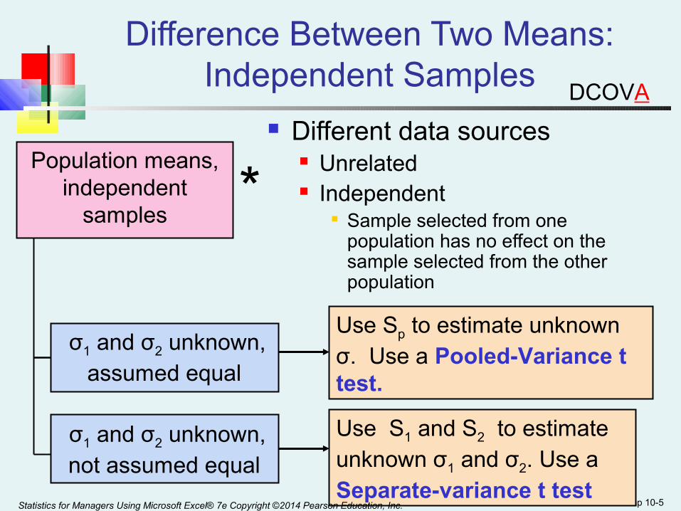
Population means, independent
samples*
Use Sp to estimate unknown σ. Use a Pooled-Variance t test.
σ1 and σ2 unknown, assumed equal
σ1 and σ2 unknown, not assumed equal
Use S1 and S2 to estimate unknown σ1 and σ2. Use a Separate-variance t test
Different data sources Unrelated Independent
Sample selected from one population has no effect on the sample selected from the other population
Statistics for Managers Using Microsoft Excel® 7e Copyright ©2014 Pearson Education, Inc.
DCOVA

Chap 10-6
Hypothesis Tests forTwo Population Means
Lower-tail test:
H0: μ1 ≥ μ2
H1: μ1 < μ2
i.e.,
H0: μ1 – μ2 ≥ 0H1: μ1 – μ2 < 0
Upper-tail test:
H0: μ1 ≤ μ2
H1: μ1 > μ2
i.e.,
H0: μ1 – μ2 ≤ 0H1: μ1 – μ2 > 0
Two-tail test:
H0: μ1 = μ2
H1: μ1 ≠ μ2
i.e.,
H0: μ1 – μ2 = 0H1: μ1 – μ2 ≠ 0
Two Population Means, Independent Samples
Statistics for Managers Using Microsoft Excel® 7e Copyright ©2014 Pearson Education, Inc.
DCOVA
Chap 10-7
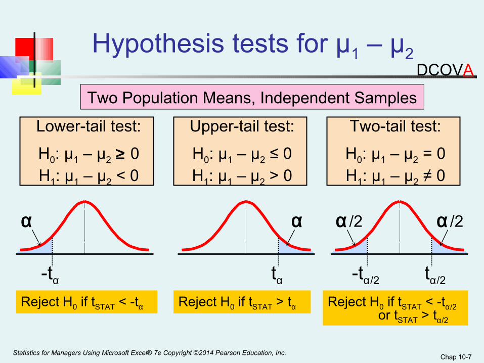
Two Population Means, Independent Samples
Lower-tail test:
H0: μ1 – μ2 ≥ 0H1: μ1 – μ2 < 0
Upper-tail test:
H0: μ1 – μ2 ≤ 0H1: μ1 – μ2 > 0
Two-tail test:
H0: μ1 – μ2 = 0H1: μ1 – μ2 ≠ 0
α α /2 α /2α
-tα -tα/2tα tα/2
Reject H0 if tSTAT < -tα Reject H0 if tSTAT > tα Reject H0 if tSTAT < -tα/2
or tSTAT > tα/2
Hypothesis tests for μ1 – μ2
Statistics for Managers Using Microsoft Excel® 7e Copyright ©2014 Pearson Education, Inc.
DCOVA
Chap 10-8
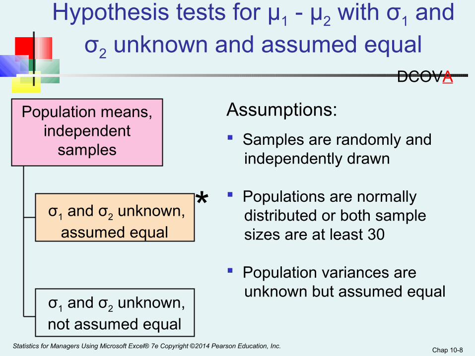
Population means, independent
samples
Hypothesis tests for µ1 - µ2 with σ1 and σ2 unknown and assumed equal
Assumptions:
Samples are randomly and independently drawn
Populations are normally distributed or both sample sizes are at least 30
Population variances are unknown but assumed equal
*σ1 and σ2 unknown, assumed equal
σ1 and σ2 unknown, not assumed equal
Statistics for Managers Using Microsoft Excel® 7e Copyright ©2014 Pearson Education, Inc.
DCOVA

Chap 10-9
Population means, independent
samples
• The pooled variance is:
• The test statistic is:
• Where tSTAT has d.f. = (n1 + n2 – 2)
(continued)
( ) ( )1)n(n
S1nS1nS
21
222
2112
p −+−−+−=
()1
*σ1 and σ2 unknown, assumed equal
σ1 and σ2 unknown, not assumed equal
Hypothesis tests for µ1 - µ2 with σ1 and σ2 unknown and assumed equal
( ) ( )
+
−−−=
21
2p
2121STAT
n
1
n
1S
μμXXt
Statistics for Managers Using Microsoft Excel® 7e Copyright ©2014 Pearson Education, Inc.
DCOVA

Chap 10-10
Population means, independent
samples
( )
+±−
21
2p/221
n
1
n
1SXX αt
The confidence interval for μ1 – μ2 is:
Where tα/2 has d.f. = n1 + n2 – 2
*
Confidence interval for µ1 - µ2 with σ1 and σ2 unknown and assumed equal
σ1 and σ2 unknown, assumed equal
σ1 and σ2 unknown, not assumed equal
Statistics for Managers Using Microsoft Excel® 7e Copyright ©2014 Pearson Education, Inc.
DCOVA
Chap 10-11
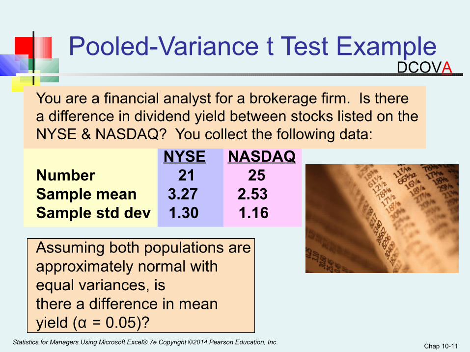
Pooled-Variance t Test Example
You are a financial analyst for a brokerage firm. Is there a difference in dividend yield between stocks listed on the NYSE & NASDAQ? You collect the following data:
NYSE NASDAQNumber 21 25Sample mean 3.27 2.53Sample std dev 1.30 1.16
Assuming both populations are approximately normal with equal variances, isthere a difference in meanyield (α = 0.05)?
Statistics for Managers Using Microsoft Excel® 7e Copyright ©2014 Pearson Education, Inc.
DCOVA
Chap 10-12
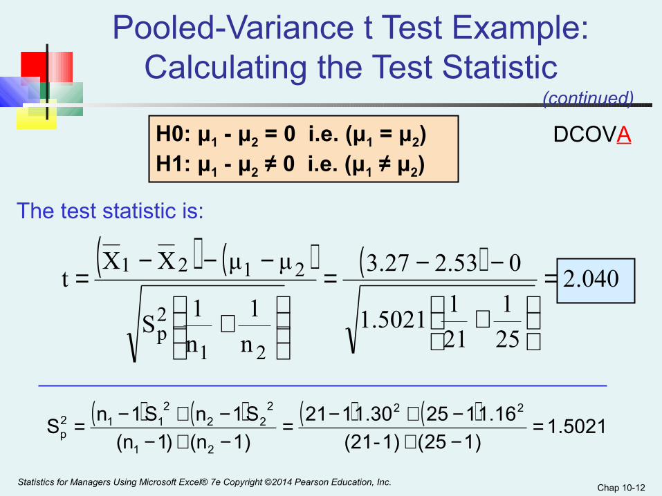
Pooled-Variance t Test Example: Calculating the Test Statistic
( ) ( ) ( ) ( )1.5021
1)25(1)-(21
1.161251.30121
1)n()1(n
S1nS1nS
22
21
222
2112
p =−+−+−=
−+−−+−=
( ) ( ) ( )2.040
25
1
21
15021.1
02.533.27
n
1
n
1S
μμXXt
21
2p
2121 =
+
−−=
+
−−−=
The test statistic is:
(continued)
H0: μ1 - μ2 = 0 i.e. (μ1 = μ2)H1: μ1 - μ2 ≠ 0 i.e. (μ1 ≠ μ2)
Statistics for Managers Using Microsoft Excel® 7e Copyright ©2014 Pearson Education, Inc.
DCOVA

Chap 10-13
Pooled-Variance t Test Example: Hypothesis Test Solution
H0: μ1 - μ2 = 0 i.e. (μ1 = μ2)
H1: μ1 - μ2 ≠ 0 i.e. (μ1 ≠ μ2)
α = 0.05
df = 21 + 25 - 2 = 44Critical Values: t = ± 2.0154
Test Statistic: Decision:
Conclusion:
Reject H0 at α = 0.05
There is evidence of a difference in means.
t0 2.0154-2.0154
.025
Reject H0 Reject H0
.025
2.040
2.040
251
211
5021.1
2.533.27t =
+
−=
Statistics for Managers Using Microsoft Excel® 7e Copyright ©2014 Pearson Education, Inc.
DCOVA
Chap 10-14
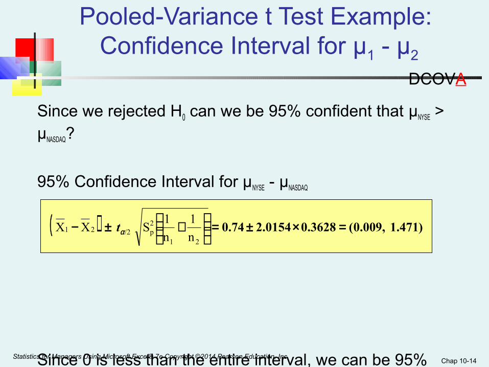
Pooled-Variance t Test Example: Confidence Interval for µ1 - µ2
Since we rejected H0 can we be 95% confident that µNYSE > µNASDAQ?
95% Confidence Interval for µNYSE - µNASDAQ
Since 0 is less than the entire interval, we can be 95% confident that µNYSE > µNASDAQ
( ) )471.1,009.0(3628.00154.274.0 n
1
n
1SXX
21
2p/221 =×±=
+±− αt
Statistics for Managers Using Microsoft Excel® 7e Copyright ©2014 Pearson Education, Inc.
DCOVA

Chap 10-15
Population means, independent
samples
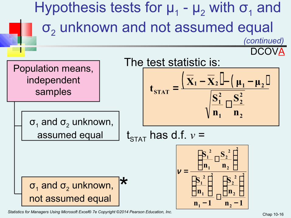
Hypothesis tests for µ1 - µ2 with σ1 and σ2 unknown, not assumed equal
Assumptions:
Samples are randomly and independently drawn
Populations are normally distributed or both sample sizes are at least 30
Population variances are unknown and cannot be assumed to be equal*
σ1 and σ2 unknown, assumed equal
σ1 and σ2 unknown, not assumed equal
Statistics for Managers Using Microsoft Excel® 7e Copyright ©2014 Pearson Education, Inc.
DCOVA
Chap 10-16
Population means, independent
samples
(continued)
*
σ1 and σ2 unknown, assumed equal
σ1 and σ2 unknown, not assumed equal
Hypothesis tests for µ1 - µ2 with σ1 and σ2 unknown and not assumed equal
The test statistic is:
( ) ( )
2
22
1
21
2121
STAT
nS
nS
μμXXt
+
−−−=
tSTAT has d.f. ν =
1n
nS
1n
nS
nS
nS
2
2
2
22
1
2
1
21
2
2
22
1
21
−
+−
+
=ν
DCOVA
Statistics for Managers Using Microsoft Excel® 7e Copyright ©2014 Pearson Education, Inc.
Chap 10-17
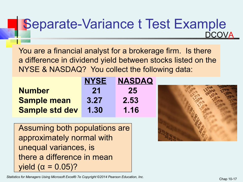
Separate-Variance t Test Example
You are a financial analyst for a brokerage firm. Is there a difference in dividend yield between stocks listed on the NYSE & NASDAQ? You collect the following data:
NYSE NASDAQNumber 21 25Sample mean 3.27 2.53Sample std dev 1.30 1.16
Assuming both populations are approximately normal with unequal variances, isthere a difference in meanyield (α = 0.05)?
Statistics for Managers Using Microsoft Excel® 7e Copyright ©2014 Pearson Education, Inc.
DCOVA
Chap 10-18
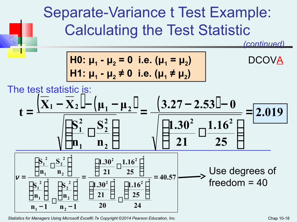
Separate-Variance t Test Example: Calculating the Test Statistic
( ) ( ) ( )2.019
251.16
211.30
02.533.27
nS
nS
μμXXt
22
2
22
1
21
2121 =
+
−−=
+
−−−=
The test statistic is:
(continued)
H0: μ1 - μ2 = 0 i.e. (μ1 = μ2)H1: μ1 - μ2 ≠ 0 i.e. (μ1 ≠ μ2)
Statistics for Managers Using Microsoft Excel® 7e Copyright ©2014 Pearson Education, Inc.
DCOVA
57.40
24
251.16
20
211.30
251.16
211.30
1n
nS
1n
nS
nS
nS
2222
222
2
2
2
22
1
2
1
21
2
2
22
1
21
=
+
+
=
−
+−
+
=νUse degrees offreedom = 40

Chap 10-19
Separate-Variance t Test Example: Hypothesis Test Solution
H0: μ1 - μ2 = 0 i.e. (μ1 = μ2)
H1: μ1 - μ2 ≠ 0 i.e. (μ1 ≠ μ2)
α = 0.05
df = 40Critical Values: t = ± 2.021
Test Statistic:Decision:
Conclusion:
Fail To Reject H0 at α = 0.05
There is no evidence of a difference in means.
t0 2.021-2.021
.025
Reject H0 Reject H0
.025
2.019
2.019t =
Statistics for Managers Using Microsoft Excel® 7e Copyright ©2014 Pearson Education, Inc.
DCOVA

Chap 10-20
Related PopulationsThe Paired Difference Test
Tests Means of 2 Related Populations Paired or matched samples Repeated measures (before/after) Use difference between paired values:
Eliminates Variation Among Subjects Assumptions:
The difference is Normally Distributed Or, if not Normal, use large samples
Related samples
Di = X1i - X2i
Statistics for Managers Using Microsoft Excel® 7e Copyright ©2014 Pearson Education, Inc.
DCOVA

Chap 10-21
Related PopulationsThe Paired Difference Test
The ith paired difference is Di , whereRelated samples
Di = X1i - X2i
The point estimate for the paired difference population mean μD is D : n
DD
n
1ii∑
==
n is the number of pairs in the paired sample
1n
)D(DS
n
1i
2i
D −
−=
∑=
The sample standard deviation is SD
(continued)
Statistics for Managers Using Microsoft Excel® 7e Copyright ©2014 Pearson Education, Inc.
DCOVA
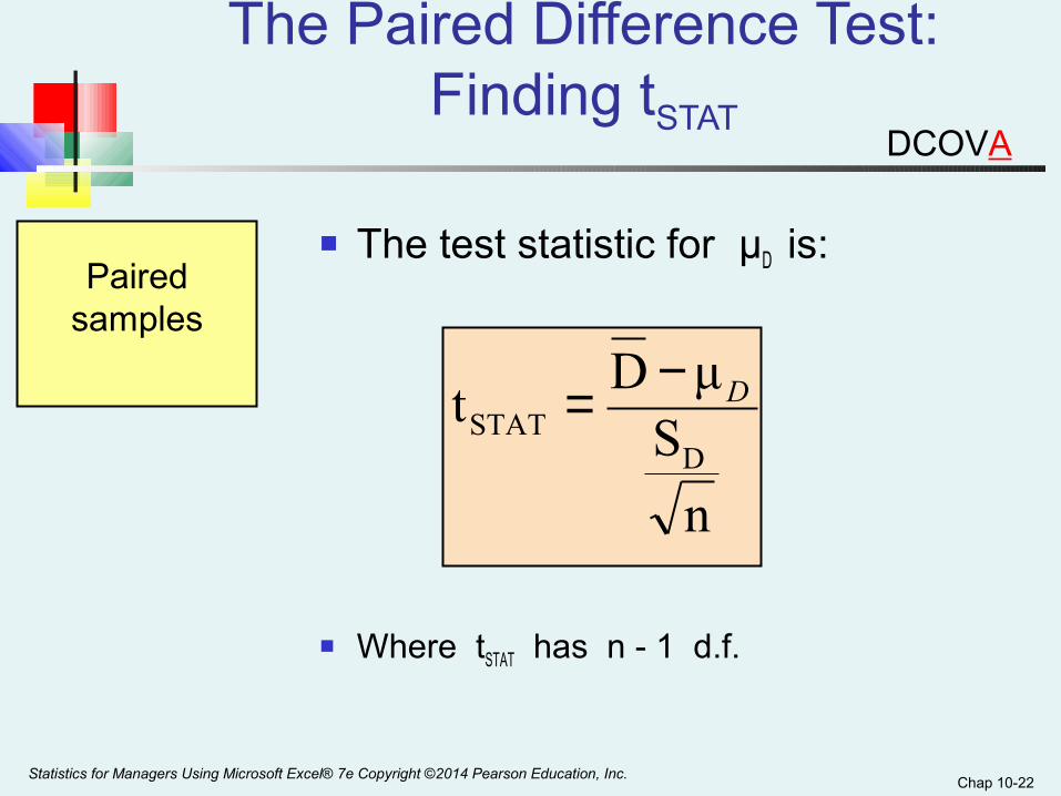
Chap 10-22
The test statistic for μD is:Paired
samples
n
SμD
tD
STATD−=
Where tSTAT has n - 1 d.f.
The Paired Difference Test:Finding tSTAT
Statistics for Managers Using Microsoft Excel® 7e Copyright ©2014 Pearson Education, Inc.
DCOVA
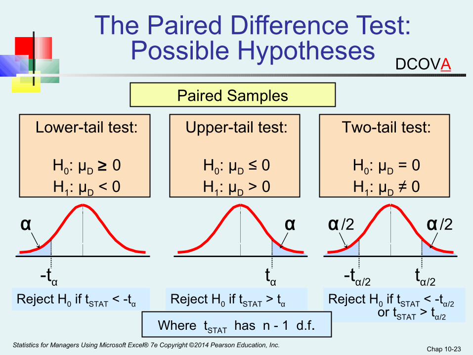
Chap 10-23
Lower-tail test:
H0: μD ≥ 0H1: μD < 0
Upper-tail test:
H0: μD ≤ 0H1: μD > 0
Two-tail test:
H0: μD = 0H1: μD ≠ 0
Paired Samples
The Paired Difference Test: Possible Hypotheses
α α /2 α /2α
-tα -tα/2tα tα/2
Reject H0 if tSTAT < -tα Reject H0 if tSTAT > tα Reject H0 if tSTAT < -tα/2
or tSTAT > tα/2 Where tSTAT has n - 1 d.f.
Statistics for Managers Using Microsoft Excel® 7e Copyright ©2014 Pearson Education, Inc.
DCOVA

Chap 10-24
The confidence interval for μD isPaired samples
1n
)D(DS
n
1i
2i
D −
−=
∑=
n
SD2/αtD ±
where
The Paired Difference Confidence Interval
Statistics for Managers Using Microsoft Excel® 7e Copyright ©2014 Pearson Education, Inc.
DCOVA

Chap 10-25
Assume you send your salespeople to a “customer service” training workshop. Has the training made a difference in the number of complaints? You collect the following data:
Paired Difference Test: Example
Number of Complaints: (2) - (1)Salesperson Before (1) After (2) Difference, Di
C.B. 6 4 - 2 T.F. 20 6 -14 M.H. 3 2 - 1 R.K. 0 0 0 M.O. 4 0 - 4 -21
D =Σ Di
n
5.67
1n
)D(DS
2i
D
=
−−
= ∑
= -4.2
Statistics for Managers Using Microsoft Excel® 7e Copyright ©2014 Pearson Education, Inc.
DCOVA
Chap 10-26
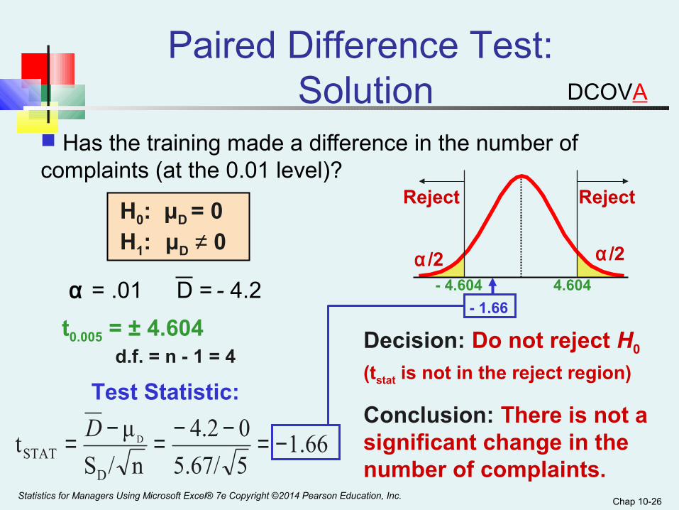
Has the training made a difference in the number of complaints (at the 0.01 level)?
- 4.2D =
1.6655.67/
04.2
n/S
μt
D
STATD −=−−=−= D
H0: μD = 0H1: μD ≠ 0
Test Statistic:
t0.005 = ± 4.604 d.f. = n - 1 = 4
Reject
α /2
- 4.604 4.604
Decision: Do not reject H0
(tstat is not in the reject region)
Conclusion: There is not a significant change in the number of complaints.
Paired Difference Test: Solution
Reject
α /2
- 1.66α = .01
Statistics for Managers Using Microsoft Excel® 7e Copyright ©2014 Pearson Education, Inc.
DCOVA
Chap 10-27
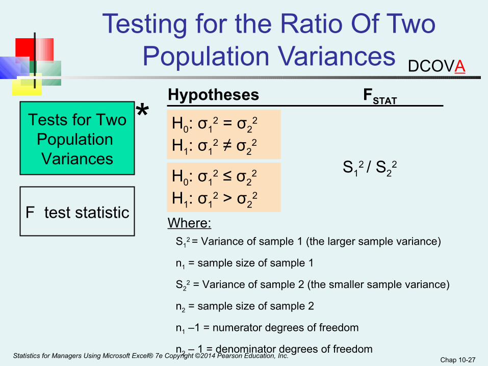
Testing for the Ratio Of Two Population Variances
Tests for TwoPopulation Variances
F test statistic
H0: σ12 = σ2
2
H1: σ12 ≠ σ2
2
H0: σ12 ≤ σ2
2
H1: σ12 > σ2
2
*Hypotheses FSTAT
S12 / S2
2
S12 = Variance of sample 1 (the larger sample variance)
n1 = sample size of sample 1
S22 = Variance of sample 2 (the smaller sample variance)
n2 = sample size of sample 2
n1 –1 = numerator degrees of freedom
n2 – 1 = denominator degrees of freedom
Where:
Statistics for Managers Using Microsoft Excel® 7e Copyright ©2014 Pearson Education, Inc.
DCOVA
Chap 10-28
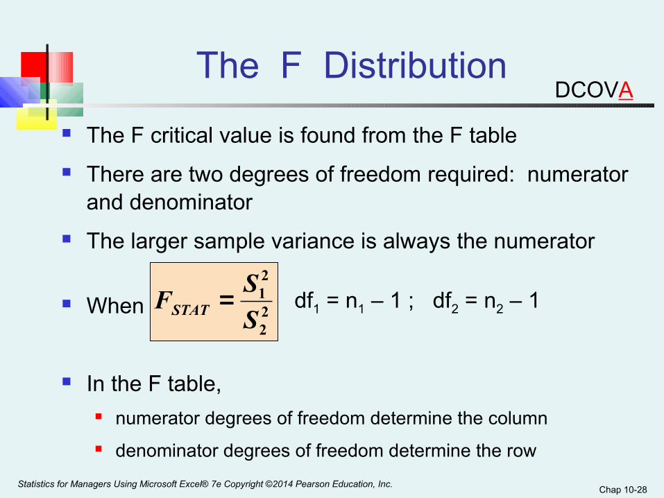
The F critical value is found from the F table
There are two degrees of freedom required: numerator and denominator
The larger sample variance is always the numerator
When
In the F table, numerator degrees of freedom determine the column
denominator degrees of freedom determine the row
The F Distribution
df1 = n1 – 1 ; df2 = n2 – 122
21
S
SFSTAT =
Statistics for Managers Using Microsoft Excel® 7e Copyright ©2014 Pearson Education, Inc.
DCOVA
Chap 10-29
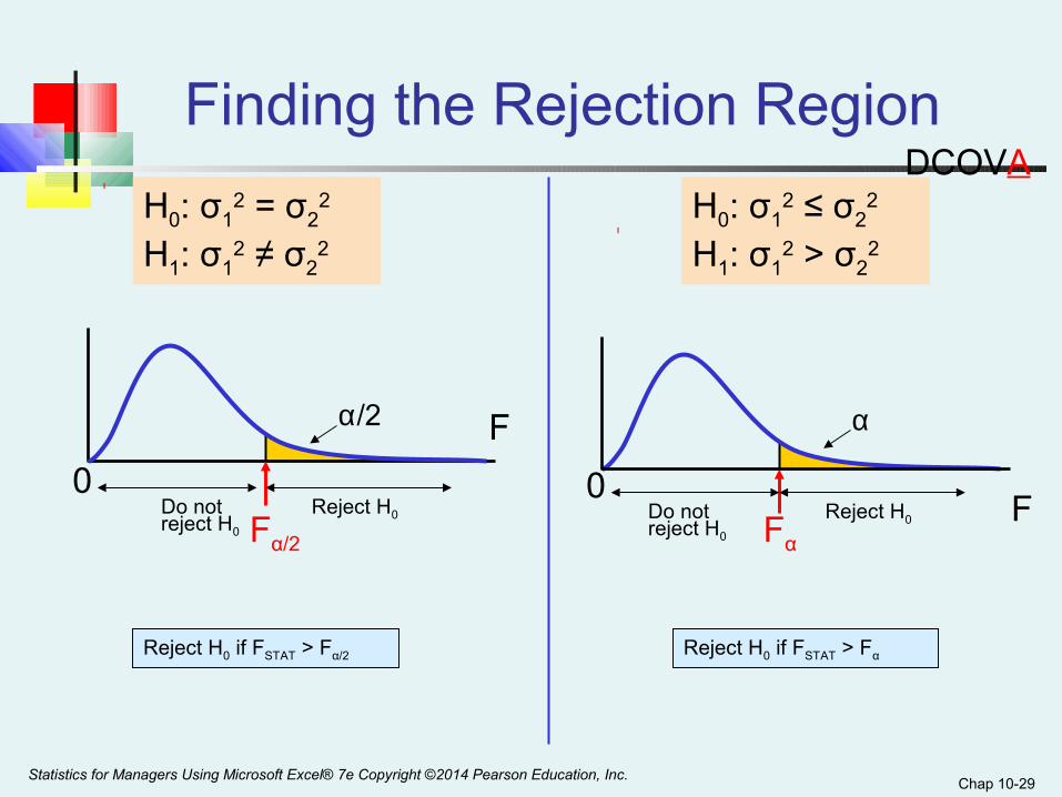
Finding the Rejection Region
H0: σ12 = σ2
2
H1: σ12 ≠ σ2
2
H0: σ12 ≤ σ2
2
H1: σ12 > σ2
2
F 0 α
Fα Reject H0Do not
reject H0
Reject H0 if FSTAT > Fα
F 0
α/2
Reject H0Do not reject H0 Fα/2
Reject H0 if FSTAT > Fα/2
Statistics for Managers Using Microsoft Excel® 7e Copyright ©2014 Pearson Education, Inc.
DCOVA
Chap 10-30
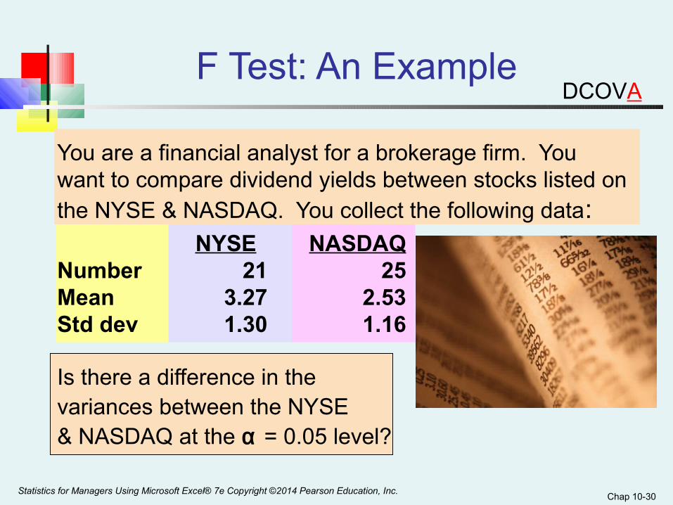
F Test: An Example
You are a financial analyst for a brokerage firm. You want to compare dividend yields between stocks listed on the NYSE & NASDAQ. You collect the following data: NYSE NASDAQNumber 21 25Mean 3.27 2.53Std dev 1.30 1.16
Is there a difference in the variances between the NYSE & NASDAQ at the α = 0.05 level?
Statistics for Managers Using Microsoft Excel® 7e Copyright ©2014 Pearson Education, Inc.
DCOVA

Chap 10-31
F Test: Example Solution
Form the hypothesis test:
H0: σ21 = σ2
2 (there is no difference between variances)
H1: σ21 ≠ σ2
2 (there is a difference between variances)
Find the F critical value for α = 0.05:
Numerator d.f. = n1 – 1 = 21 –1 =20
Denominator d.f. = n2 – 1 = 25 –1 = 24
Fα/2 = F.025, 20, 24 = 2.33
Statistics for Managers Using Microsoft Excel® 7e Copyright ©2014 Pearson Education, Inc.
DCOVA
Chap 10-32
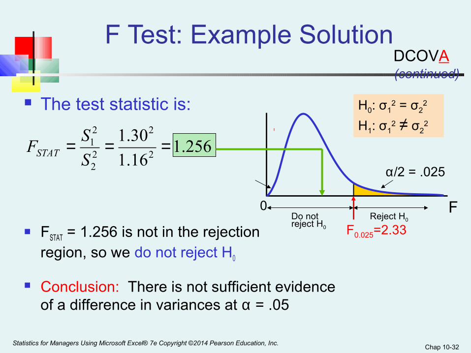
The test statistic is:
0
256.116.1
30.12
2
22
21 ===S
SFSTAT
α/2 = .025
F0.025=2.33Reject H0Do not
reject H0
H0: σ12 = σ2
2
H1: σ12 ≠ σ2
2
F Test: Example Solution
FSTAT = 1.256 is not in the rejection region, so we do not reject H0
(continued)
Conclusion: There is not sufficient evidence of a difference in variances at α = .05
F
Statistics for Managers Using Microsoft Excel® 7e Copyright ©2014 Pearson Education, Inc.
DCOVA
Chap 10-33
Chapter Summary
In this chapter we discussed Comparing two independent samples
Performed pooled-variance t test for the difference in two means
Performed separate-variance t test for difference in two means
Formed confidence intervals for the difference between two means
Comparing two related samples (paired samples) Performed paired t test for the mean difference Formed confidence intervals for the mean difference
Statistics for Managers Using Microsoft Excel® 7e Copyright ©2014 Pearson Education, Inc.
Chap 10-34
Chapter Summary
Performing an F test for the ratio of two population variances
(continued)
Statistics for Managers Using Microsoft Excel® 7e Copyright ©2014 Pearson Education, Inc.