Two Forecasting Modelsfor Portland, Oregon

Hamilton – Perry vs Metroscope

Richard Lycan

Senior Research Associate

Institute on Aging, Portland State University

Association of American Geographers

Boston, Massachusetts

April, 2017

Background for paper

• At a planning meeting for the Multnomah Co. program for Aging, Veterans and Disability services:

• A planner for the program asked: Are the recentforecasts by the PSU Center for Population Research thebest available on which to base our planning?

• I replied: Probably, but you should look at Metro’sMetroscope forecast as well --- however

• Access to the details of Metro’s forecast a problem.

• Those needing demographic forecasts needed to ask Metro to provide the details.

• Development of the Metroscope Query tool, a Excel VBA application.

• The Hamilton-Perry population and forecast is used as baseline forecast to evaluate forecasts from Metroscope.

Background on Portland Population and Housing

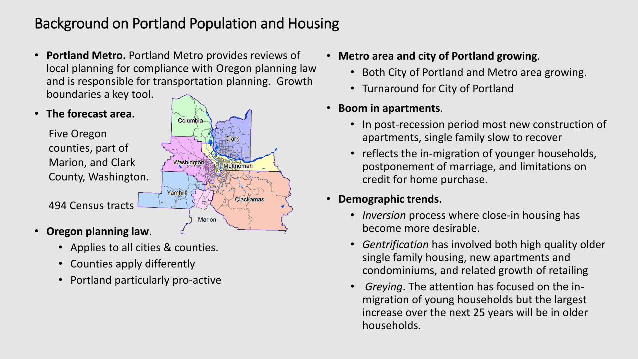
• Portland Metro. Portland Metro provides reviews of local planning for compliance with Oregon planning law and is responsible for transportation planning. Growth boundaries a key tool.

• The forecast area.

• Oregon planning law.

• Applies to all cities & counties.

• Counties apply differently

• Portland particularly pro-active

• Metro area and city of Portland growing.

• Both City of Portland and Metro area growing.

• Turnaround for City of Portland

• Boom in apartments.

• In post-recession period most new construction of apartments, single family slow to recover

• reflects the in-migration of younger households, postponement of marriage, and limitations on credit for home purchase.

• Demographic trends.

• Inversion process where close-in housing has become more desirable.

• Gentrification has involved both high quality older single family housing, new apartments and condominiums, and related growth of retailing

• Greying. The attention has focused on the in-migration of young households but the largest increase over the next 25 years will be in older households.

Five Oregon counties, part of Marion, and Clark County, Washington.

494 Census tracts

• Focus on City of Portland and surrounding Oregon counties.

• City of Portland in yellow shade.

• Grey shades show urban growth boundary (UGB)

• Dark – original 1974 UGB boundaries

• Mid – out to current UGB

• Light – Outside the UBG, rural

• Single family housing units by year built. Recently built in red.

• Multiple family housing units by year built.

• Small developments

• Large developments

• Both..

The Portland Tour

The Metroscope Forecasting Model

Metro’s Metroscope model

• Belongs to a class of metropolitan transportation models, e.g. Empiric. An urban simulation model of the Herbert-Stevens type.

• Originally developed to support transportation planning.

• Used for 25 year forecast of land needed for urban development as required under Oregon land use planning law.

• Complex, developed locally by Metro.

A. Tenure computation by HIA class:

PRCNTOWN™ = {EXP{-b0 - bx (AGEHD) + b2

(AGEHDSQ) - b, (INC) + b4 (INCSQ) j + b5(HSZE) +

b6(RX)-b1(HX)-bB(TX))}/{\ bx (A GEHD) + b2

(AGEHDSQ) - b3 (INC) + b4 (INCSQ) + b5 (HSZE) +

b6 (RX) - bn (HX) - b, (TX))}

2.) PRCNTRENTHIA = [1 -PRCNTOWNH1A]

B. House price and monthly rent computation by

HIA class:

OWN:PRC?'A =({EXP(bo +b1(AGEHD)-b2(AGESQ)-

bJ(INC) + b4 (INCSQ) - bs (HSZE) + b6 (RX) + b7

(TX))} /{I + EXP(bo - bx (AGEHD) + b2 (A GESQ) - b3

(INC) + i>4 (INCSQ) - b5 (HSZE) + b6 (RX) + bn

(TX))]}) (MAXPRQ(PRCIKEQUILIBRIUMMULTIPLIER)

RENT: MRENT,HIA - {{EXP(b0 - bx (A GEHD) + b2 (A

GEHSQ) - b3 (INC) + b4 (INCSQ) + b5 (HSZE) + b6

(HX) - b, (TX))} /{I + EXP(b0 - b{ (AGEHD) 4.) + b2 (A

GESQ) - b3 (INC) + b4 (INCSQ) + b5 (HSZE) + b6

Overview Under the hood a shoe box full of:

Metroscope data not very accessible - The Metroscope query tool

• A query tool was built in Excel to generate tables from the Metroscope forecast data.

• In this example data are extracted for lower income households, with or without children present, all household sizes and householder age 65+.

• The data can be viewed in tabular form in a variety of ways or exported.

• The tabulations show population or households by type and tenure.

• The tool even has some mapping tools added to Excel, here showing household size for condos and apartments for the same KHIA classes.

The Hamilton – Perry Model

2000 and 2010 total population in households for five year age groups

The cohort progression ratios

Tract is 203.03 lies within Oregon PUMA 1309

Allocation table persons by age of to age of householder 2008-2012 using

five year ACS PUMS

Forecast of number of households by age of

householder for census tract 202.03.

The Hamilton-Perry Model

Matrix multiply converts Hamilton-Perry persons by age to Metroscope households by age of householder.

10 year population forecast , using cohort progression ratios above.

Blue data lines are interpolated for “5” years.

The Hamilton – Perry Forecasting Model

290214

Census tract 203.03

• The Metroscope forecast model covered seven counties or parts of counties that included 484 2010 census tracts.

• To make Hamilton-Perry work one needs exactly equivalent geographies for the two time periods, here 2000 and 2010.

• Merging of tracts backward from 2010 to 2000 resulted in 424 comparable 2000 to 2010 tracts.

Making 2000 and 2010 Geographies Comparable

Metroscope versus Hamilton-Perry

• Metroscope – Metro’s forecasting model• A complicated urban simulation model.• Provides socio-economic detail: households by age, income,

housing type and tenure, and presence of children.

• Hamilton-Perry – An abbreviated cohort component model• Requires only age-sex detail from two censuses and no

assumptions about birth and death rates.• Provides only age/sex detail by age group.

• Why do we care?• The results of the two forecasts for Portland are very different.• Local organizations depend on population forecasts as a basis for

their organizational planning.• Some demographers argue that simple models forecast as well as

complex ones and have some supporting evidence with respect to the Hamilton-Perry model.

How did the forecasts by Metroscope and Hamilton-Perry compare?

The simple answer is that they vary considerably. This poses both methodological and practical problems.

Households20352010

%

--- 62

--- 78

--- 92

--- 108

--- 128

--- 164

--- 222

--- 323

--- 555

Metroscopeas Percent ofHamilton-Perry

--- 5

--- 47

--- 79

--- 103

--- 126

--- 156

--- 203

--- 281

--- 475

All Age Groups

• The Hamilton-Perry model forecasts slower or negative growth for Portland and the inner suburbs such as Beaverton and Lake Oswego. It forecasts modest growth in the inner suburbs.

• Metroscope by contrast forecasts higher growth in the City of Portland and in the outer suburbs.

• This map shows the ratio of growth rates for Metroscope as a percent of those for the Hamilton-Perry model.

• It shows Metroscope forecasting higher growth for Portland but also for some of the inner and outer suburbs.

• 15-24. MS forecasts more growth for this cohort in City and in inner suburbs. Hamilton-Perry forecasts decline in central east side of City.

• 25-44. HP forecasts decline in inner east side of City whereas MS forecasts growth in some tracts. HP shows decline in Clackamas Co. but MS shows growth.

• 45-64. MS forecasts growth of most of City whereas HP mainly forecasts declines for this area.

• 65+. Both models forecast high growth for older households in most areas, higher for MS. Lower growth forecast by MS in some inner suburbs.

Households by age of householder

MS = MetroscopeHP = Hamilton-PerryGreen outline – City of Portland

All maps scaled to same colors

Why are the Metroscope and Hamilton-Perry forecasts so different?

• Overall and for age groups the scatter diagrams showed near zero correlations between Metroscope and Hamilton-Perry at the census tract level.

• Some possible reasons

• The base period for the forecast, 2000 – 2010 included a recession and sharp decline in housing construction.

• In the post recession period there has been a major shift from single family to apartment and condo construction.

• Oregon’s growth boundary law may have resulted in sudden bursts of housing construction when new developable areas became available.

• Portland planning has been very pro-active in fostering housing development to counteract shortages.

R2=0.048

Met

rosc

op

e

Hamilton-Perry

The recession and post-recession shift in housing mix

• For three of the Oregon counties we can document the decline in housing construction during the recession and the shift to multi-family post recession.

• The shift in housing mix was greatest in Multnomah Co. which includes the City of Portland.

• I expected that the difference between the two forecasts might have been related to housing mix and change in housing mix.

• However reality intruded and the tract level correlations were near zero, the highest being 0.23 between the absolute change and the percent of housing that was multifamily (from tax-lot and multifamily housing inventory data).

We can not explain the differences between the Hamilton-Perry and Metroscope forecasts based on housing mix and changes in housing mix during the base period for the forecast.

• A possible reason for the differences might be the growth trajectories in the census tracts that were opened to development as the growth boundary expanded.

• If the development in these tracts followed a logistic curve, forecasts made when the development was at one of the two inflection points growth might be over or under forecast.

• Tract 302 shown here was at the upper inflection point, but the two forecasts were not very different.

• I examined a number of census tracts and the evidence was mixed. Also these tracts are large in square miles and there are not very many of them.

Odd growth trends in the tracts along the urban growth boundary could have had only a small impact on the differences between the Metroscope and Hamilton-Perry forecasts.

For this UGA largely built-out expansion tract single family units approximate a logistic curve reasonably well. Multi-family reached its maximum in about 1975. The Metroscope and Hamilton-Perry forecasts are relatively similar.

• The City of Portland has been undergoing several different flavors of gentrification all of which indicate a shift away from earlier trends – an argument against the Hamilton-Perry model.

• This slide shows tracts undergoing residential gentrification based on increase in educational levels and professional employment (after David Ley).

• Along with residential gentrification there has been upscaling of commercial activities and accompanying apartment and condo development along major arterials.

• The Metroscope forecast provides considerable detail on housing type and tenure which allows us to consider the logical basis for the forecast.

However the urban development process is multi-dimensioned and difficult to operationalize to compare the two forecasting models.

Conclusions and next steps• Conclusions

• The wide differences between Metroscope and the Hamilton-Perry forecasts is concerning.• Forecasts needed by local organizations.• Raises questions about Hamilton-Perry.• Metroscope forecast more spatially complex.• Numbers thin for trends based on 5 year age

groups using Hamilton-Perry.

• Is one forecast more right?• Metroscope uses detailed GIS data to localize

forecast, vacant lands and redevelopment potential.

• Metroscope is based on assumptions about land use policy. Forecasts more growth for City of Portland. Governments change and policies change. New forecasts will differ.

• Hamilton-Perry forecast based on recent population trends. It serves a useful purpose as a baseline forecast. May misread logistic trends.

• Next steps• Update Metroscope query tool to make use of

2040 forecast and 2040 post local review.

• Encourage use of tool and Metroscope forecasts by local organizations and by planning students at PSU.

• Re-do calculations. Use ten year age groups to stabilize cohort progression ratios.

• Further analyze differences between two forecasts using tract level census and land use variables to attempt find explanation for differences – not there yet!

AcknowledgementsThanks to Portland Metro for assistance with the Metroscope forecast and the supporting RLIS GIS data. I also wish to acknowledge the mentoring of the several past directors of the Portland State University Population Research Center.

Richard Lycan, Institute on AgingPortland State University, Portland, Oregon lycand@pdx.edu