two-dimensional numerical modeling of radio...
TRANSCRIPT
Two-Dimensional Numerical Modeling of Radio-Frequency Ion Engine Discharge
Michael Meng-Tsuan Tsay, Manuel Martinez-Sanchez
August 2010 SSL # 14-10

2
3
Two-Dimensional Numerical Modeling of Radio-Frequency Ion Engine Discharge
Michael Meng-Tsuan Tsay, Manuel Martinez-Sanchez
August 2010 SSL # 14-10
This work is based on the unaltered text of the thesis by Michael Meng-Tsuan Tsay submitted to the Department of Aeronautics and Astronautics in partial fulfillment of the requirements for the degree of doctor of philosophy at the Massachusetts Institute of Technology.

4

5
Two-Dimensional Numerical Modeling of Radio-Frequency Ion Engine Discharge
by
Michael Meng-Tsuan Tsay
Submitted to the Department of Aeronautics and Astronautics
on August 19, 2010 in partial fulfillment of the requirements for the degree of Doctor of Philosophy in
Aeronautics and Astronautics in the field of Space Propulsion ABSTRACT Small satellites are gaining popularity in the space industry and reduction in spacecraft size requires scaling down its propulsion system. Low-power electric propulsion poses a unique challenge due to various scaling penalties. Of high-performance plasma thrusters, the radio-frequency ion engine is most likely to succeed in scaling as it does not require an externally applied magnetic field and is structurally simple to construct. As part of a design package an original two-dimensional simulation code for radio-frequency ion engine discharge is developed. The code models the inductive plasma with fluid assumption and resolves the electromagnetic wave in the time domain. Major physical effects considered include magnetic field diffusion and coupling, plasma current induction and ambipolar plasma diffusion. The discharge simulation is benchmarked with data from an experimental thruster. It shows excellent performance in predicting the load power and the internal power loss of the plasma. Predictability of anode current depends on the operating power but is generally adequate. Optimum skin depth on the order of half of chamber radius is suggested by the simulation. The code also demonstrates excellent scaling ability as it successfully predicts the performance of a smaller thruster with errors less than 10%. Using the code a brief optimization study was conducted and the results suggest the maximum thrust efficiency does not necessarily occur at the same frequency that maximizes the power coupling efficiency of the matching circuit. Thesis Supervisor: Manuel Martinez-Sanchez Title: Professor of Aeronautics and Astronautics

6
Acknowledgement This thesis work was partially funded by Busek Co., Inc. as a subcontract to Busek’s SBIR Phase II contract with NASA/JPL (contract number NNC06CA24C).
7
Table of Contents List of Figures...................................................................................................................... 9
List of Tables ..................................................................................................................... 12 Nomenclature .................................................................................................................... 13
Chapter 1 Introduction................................................................................................... 14 1.1 RF Ion Engines.................................................................................................... 15
1.1.1 Concept and Description ........................................................................... 15 1.1.2 Advantages and Applications .................................................................... 17
1.1.3 Issues ........................................................................................................ 19 1.2 Busek RF Ion Engines ......................................................................................... 19
1.3 Previous Numerical Work.................................................................................... 21 1.4 Research Objective.............................................................................................. 22
1.5 Thesis Outline ..................................................................................................... 22 Chapter 2 Model Description ......................................................................................... 24
2.1 Fluid Approximation ........................................................................................... 25 2.2 Basic Assumptions .............................................................................................. 27
2.3 The Spatial 2D Assumption ................................................................................. 28 2.3 Computation Domain .......................................................................................... 31
2.4.1 Mesh......................................................................................................... 31 2.4.1 Time Step ................................................................................................. 32
Chapter 3 Theory............................................................................................................ 34 3.1 Transformer Model.............................................................................................. 34
3.2 ICP Discharge Model .......................................................................................... 37 3.2.1 Magnetic Field Coupling and Plasma Current Induction............................ 37
3.2.2 Plasma Conductivity ................................................................................. 41 3.2.3 Energy-Averaged Cross Sections .............................................................. 43
3.2.4 Fluid Equations......................................................................................... 47 3.2.5 Neutral Conservation ................................................................................ 49
3.2.6 Discharge Energy Balance ........................................................................ 50 3.2.7 Coil-Induced Magnetic Field..................................................................... 51
3.3 Numerical Method............................................................................................... 54 3.3.1 Boundary Conditions for Magnetic Field .................................................. 54
8
3.3.2 Bohm Condition........................................................................................ 56 3.3.3 Numerical Solution ................................................................................... 57
3.4 Ion Optics............................................................................................................ 62 Chapter 4 Results............................................................................................................ 64
4.1 Matching Circuit Design...................................................................................... 65
4.2 Performance of ICP Discharge Code ................................................................... 67
4.2.1 Convergence ............................................................................................. 67 4.2.2 BRFIT-7 Simulation ................................................................................. 72
4.2.3 BRFIT-3 Simulation ................................................................................. 82 4.3 Thruster Optimization.......................................................................................... 87
Chapter 5 Conclusion ..................................................................................................... 92 5.1 Results Summary................................................................................................. 92
5.2 Contributions....................................................................................................... 93 5.3 Recommendations for Future Work ..................................................................... 93
Appendix A Derivation of EEDF in Energy Space........................................................ 95 Appendix B Ionization Cross Section of Xenon............................................................. 99
Appendix C Excitation Cross Section of Xenon .......................................................... 100 Appendix D Derivation of Coil-Induced Magnetic Field............................................. 101
References........................................................................................................................ 106
9
List of Figures Figure 1 RIT-10 Thruster by EADS Astrium ................................................................... 15
Figure 2 Illustration of a Typical Two-Grid RF Ion Engine.............................................. 16
Figure 3 Rapid and Precise Change of Thrust by Modulating RF Power Programmed
through a Music Waveform................................................................................ 18
Figure 4 Busek 7-cm RF Ion Engine (BRFIT-7) .............................................................. 20
Figure 5 BRFIT-7 Operating at 400W Total Power on Xenon.......................................... 20
Figure 6 Busek 3-cm RF Ion Engine (BRFIT-3) .............................................................. 20
Figure 7 BRFIT-3 Operating at 100W Total Power on Xenon.......................................... 20
Figure 8 Knudsen Number Estimated for Busek BRFIT-7 Ion Engine.............................. 26
Figure 9 A Two-Turn Axisymmetric Coil ........................................................................ 29
Figure 10 A Two-Turn Helical Coil ................................................................................... 29
Figure 11 BRFIT-7 Performance Comparison Between Helical and Axisymmetric Coils with
3 sccm Xenon Flow ........................................................................................... 30
Figure 12 BRFIT-7 Performance Comparison Between Helical and Axisymmetric Coils with
4 sccm Xenon Flow ........................................................................................... 30
Figure 13 Conceptual Arrange of BRFIT-7 RF Ion Engine ................................................ 31
Figure 14 Computation Mesh Configured for BRFIT-7 Thruster (Chamber Size Not to Scale)
.......................................................................................................................... 32
Figure 15 Circuit Diagram of the Transformer Model ........................................................ 35
Figure 16 Illustration of the Special EEDF with Drift Energy, Te = 5 eV ........................... 44
Figure 17 Cross Section Data for Xenon, Collected by Szabo ............................................ 44
Figure 18 Energy-Averaged Electron-Neutral Scattering Cross Section for Xenon............. 46
Figure 19 Energy-Averaged Ionization Cross Section (Ionization Rate Coefficient
Normalized by Mean Thermal Velocity) for Xenon ........................................... 46
Figure 20 Energy-Averaged Excitation Cross Section (Excitation Rate Coefficient
Normalized by Mean Thermal Velocity) for Xenon ........................................... 47
Figure 21 Calculation of Magnetic Field at Point P Induced by Loop Current I in a
Single-Turn Coil ................................................................................................ 53
Figure 22 Baseline Coil-Induced Magnetic Field (Aθ)co with BRFIT-7 Geometry; Coil
Current is at Positive Peak (1/4 Wave) ............................................................... 54
10
Figure 23 Solution Scheme for Magnetic Boundary Condition .......................................... 55
Figure 24 Five-Point Finite-Differencing Scheme ............................................................. 58
Figure 25 Ion Transparency Simulation Published by Farnell ............................................ 63
Figure 26 Flowchart of the ICP Discharge Code................................................................ 65
Figure 27 Matching Circuit Design for BRFIT-7 with the Transformer Model; Plasma
Conductivity is Assumed 500 Si/m .................................................................... 66
Figure 28 Matching Circuit Design for BRFIT-7 with the Transformer Model; Plasma
Conductivity is Assumed 1000 Si/m .................................................................. 67
Figure 29 Convergence of Electron Temperature in the BRFIT-7 Simulation; Each Iteration
Represents 7.7×10⁻¹⁰ Seconds in Real Time ....................................................... 69
Figure 30 Convergence of Dissipated Power in the BRFIT-7 Simulation........................... 70
Figure 31 Convergence of Various Power Loss Terms in the BRFIT-7 Simulation............ 70
Figure 32 Convergence of Circuit Ohmic Heating Loss..................................................... 71
Figure 33 Convergence of Anode Current in the BRFIT-7 Simulation ............................... 71
Figure 34 Total Magnetic Vector Potential at 1/4 Wave ..................................................... 72
Figure 35 Total Magnetic Vector Potential at 3/4 Wave ..................................................... 73
Figure 36 Induced Plasma Current at 1/4 Wave ................................................................. 74
Figure 37 Induced Plasma Current at 1/2 Wave ................................................................. 74
Figure 38 Induced Plasma Current at 3/4 Wave ................................................................. 75
Figure 39 Dissipated Power at 1/4 Wave............................................................................ 76
Figure 40 Dissipated Power at 1/2 Wave............................................................................ 76
Figure 41 Dissipated Power at 3/4 Wave............................................................................ 77
Figure 42 Electric Potential Distribution............................................................................ 78
Figure 43 Electric Potential Distribution (Planar View) ..................................................... 78
Figure 44 Plasma Density Distribution............................................................................... 79
Figure 45 Plasma Density Distribution (Planar View) ........................................................ 79
Figure 46 Ion Axial Velocity Profile .................................................................................. 80
Figure 47 Simulated Ion Beam Current Density Profile ..................................................... 81
Figure 48 Ion Beam Flux Profile Measured by a Faraday Probe......................................... 81
Figure 49 Anode Current Comparison for BRFIT-7........................................................... 82
Figure 50 Knudsen Number Estimated for BRFIT-3 .......................................................... 83
Figure 51 Anode Current Comparison for BRFIT-3........................................................... 84
Figure 52 Convergence of Electron Temperature in the BRFIT-3 Simulation; Each Iteration
Represents 2.8×10⁻¹⁰ Seconds in Real Time ....................................................... 84
11
Figure 53 Convergence of Dissipated Power in the BRFIT-3 Simulation........................... 85
Figure 54 Convergence of Anode Current in the BRFIT-3 Simulation............................... 85
Figure 55 Power Distribution in BRFIT-3 and BRFIT-7.................................................... 87
Figure 56 Matching Circuit Analysis for BRFIT-3 ............................................................ 88
Figure 57 Ideal Scaling for Optimizing Thrust Efficiency of an RF Ion Engine ................. 88
Figure 58 Thrust Efficiency Optimization of BRFIT-3 ...................................................... 89
Figure 59 Plasma Dissipated Power as Function of Frequency .......................................... 90
Figure 60 Distribution of Dissipated Power with 1.8 MHz ................................................ 90
Figure 61 Distribution of Dissipated Power with 2.5 MHz ................................................ 91

12
List of Tables Table 1 Parameters for Grid Ion Transparency Simulation.............................................. 62
Table 2 Converged Values from Discharge Simulation................................................... 69
Table 3 Results Comparison for BRFIT-7 Simulation..................................................... 82
Table 4 Results Comparison for BRFIT-3 Simulation..................................................... 83
Table 5 Electric Power Distribution within BRFIT-3 and BRFIT-7 Thrusters................. 86

13
Nomenclature
A
= magnetic field vector potential, tesla-m
E
= electric field strength, volts/m
j
= electric current density, amperes/m2
= electric potential, volts
e = electron charge, 1.6x10⁻¹⁹ coulombs
k = Boltzmann constant, 1.38x10⁻²³ J/K
= electrical conductivity, siemens/m
= skin depth, m
= driving frequency, radian/s
0 = permeability of vacuum, 4π×10−7 N/m2
en = ionization rate, 1/m3/s
gn = number density of species g, 1/m3
gm = mass of species g, kilogram
eT = electron temperature, electron-volt
EEDF = electron energy distribution function CFD = computational fluid dynamics

14
Chapter 1
INTRODUCTION
Small satellites are gaining popularity in the space industry as recent technology advancement
allows manufacturers to build smaller and more cost-effective spacecraft without sacrificing
functionality. Reduction in spacecraft size requires scaling down its subsystems and reducing
their power consumption. Of the subsystems, low-power electric propulsion (EP) poses a
unique challenge due to particularly severe scaling penalties in both efficiency and
power-to-mass ratio. While non-plasma-based EP such as colloid [1,2] and field-emission
electric propulsion (FEEP) thrusters [3] can maintain high thrust efficiency regardless of scale,
they are emerging technologies that have not been proven for space flight. Plasma-based EP
such as ion engines and Hall-effect thrusters are flight proven and can offer high specific
impulse (Isp), but their efficiency decreases at reduced scale and power due to the energy
expenditure necessary for generating the plasma source and compensating ion wall loss. In
addition, the often-required magnetic structure of these thrusters does not scale well and
consequently prevents significant mass reduction.
The radio-frequency (RF) ion engine, also known as an RF ion thruster, is a type of
plasma-based electrostatic EP device that does not rely on externally applied magnetic fields to
create its plasma source. Isp performance is typically high, similar to other gridded ion
engines. Their uniqueness comes from simplicity, as no permanent magnetic structure is
required and the thruster can easily be scaled down. Such feature makes RF ion engines ideal
for small satellites that desire high-performance EP but have strict budget in volume, mass and
power. Although simple to construct, designing an RF ion engine requires thorough
knowledge of the inductively-coupled plasma (ICP) discharge and its matching circuit in order
to efficiently generate the plasma source. This thesis research aims to tackle such problem
with the goal of developing a design tool for RF ion engines.

15
1.1 RF Ion Engines
RF ion engines are related to the traditional direct-current (DC), electron-bombardment ion
engines in the sense that they both rely on electrostatic force between grids to accelerate
positively-charged heavy particles to produce thrust. High Isp and moderate efficiency are the
norm. Like most EP thrusters, performance of RF ion engines varies widely with input power
and size. Flight heritage systems exist with grid diameters up to 25 cm and power up to 6
kW[4]. Total efficiencies (thrust efficiency × propellant utilization) can easily exceed 50%
for 400W-class systems and above [5]. Depending on power level, thrust can vary from 10
mN to 200 mN with Isp ranging between 2500 and 5500 sec [6,7].
The first RF ion engine tested in space was the German RIT-10 thruster launched by the Space
Shuttle Atlantis in 1992. It served as a technology demonstrator onboard the European
Retrievable Carrier (EURECA) spacecraft. RIT-10 operated for 240 hours at 5-10 mN thrust
level and 3000 sec Isp before succumbing to an overheating problem on the RF coil. This
problem was later resolved and RIT-10 was commissioned again in 2001 onboard the
Advanced Relay Technology Mission Satellite (ARTEMIS). It operated for 7,500 hours and
helped raise ARTEMIS into its operational geostationary orbit [8,9]. Figure 1 shows the
RIT-10 thruster configured for ARTEMIS.
Figure 1 RIT-10 Thruster by EADS Astrium [9]
1.1.1 Concept and Description
An RF ion engine typically consists of an axisymmetric, cylindrical or conical discharge
chamber made of dielectric material. A helical coil, energized at low mega-hertz radio
frequency, is used to generate and sustain the plasma discharge. RF ion engines can be
equipped with two or three grids. The first grid extracts the ions and sometimes serves as
16
anode to collect electrons from the discharge. The voltage on the first grid is normally
1500-2000 V. The second grid focuses and accelerates the ion beam, while at the same time
sets up a negative potential field to prevent electrons back-streaming from the external
neutralizer. Typical voltage on the second grid is 100-200 V. The third grid, when used,
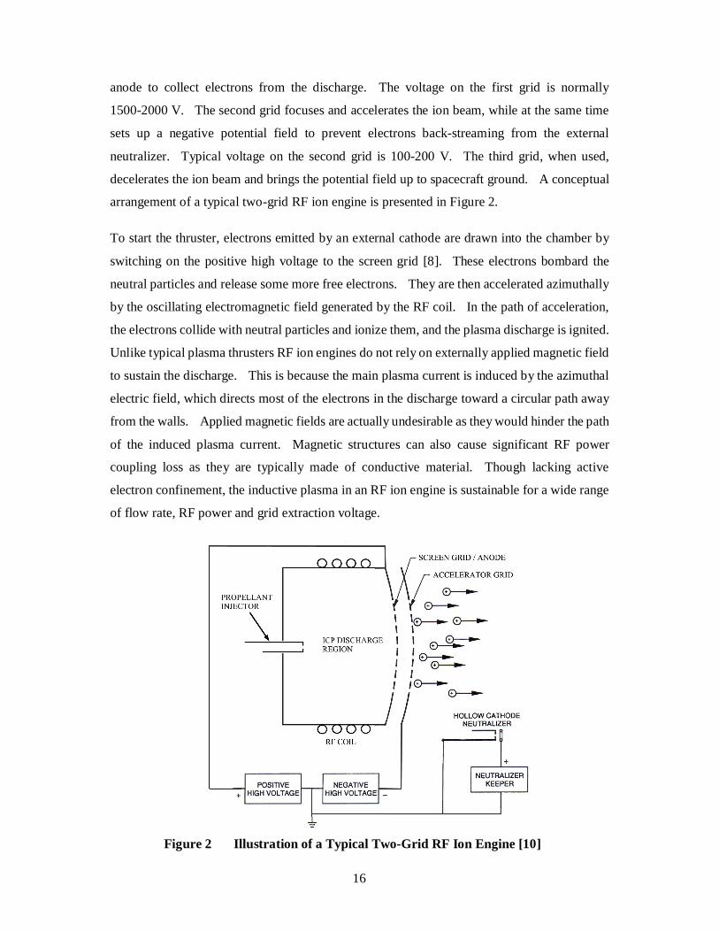
decelerates the ion beam and brings the potential field up to spacecraft ground. A conceptual
arrangement of a typical two-grid RF ion engine is presented in Figure 2.
To start the thruster, electrons emitted by an external cathode are drawn into the chamber by
switching on the positive high voltage to the screen grid [8]. These electrons bombard the
neutral particles and release some more free electrons. They are then accelerated azimuthally
by the oscillating electromagnetic field generated by the RF coil. In the path of acceleration,
the electrons collide with neutral particles and ionize them, and the plasma discharge is ignited.
Unlike typical plasma thrusters RF ion engines do not rely on externally applied magnetic field
to sustain the discharge. This is because the main plasma current is induced by the azimuthal
electric field, which directs most of the electrons in the discharge toward a circular path away
from the walls. Applied magnetic fields are actually undesirable as they would hinder the path
of the induced plasma current. Magnetic structures can also cause significant RF power
coupling loss as they are typically made of conductive material. Though lacking active
electron confinement, the inductive plasma in an RF ion engine is sustainable for a wide range
of flow rate, RF power and grid extraction voltage.
Figure 2 Illustration of a Typical Two-Grid RF Ion Engine [10]

17
The most common propellant used in RF ion engines is the noble gas xenon. Other propellants
have been experimented with, including mercury, argon and krypton. Xenon is favorable for
its low first ionization energy (12.1 eV) and high atomic weight (131.3 g/mole). The low
ionization energy contributes to more efficient usage of discharge power, and the heavy mass
would minimize loss factors for a given specific impulse [11]. Due to the heaviness, xenon
ions are seldom magnetized in the presence of permanent or induced magnetic field and
therefore can be accelerated electrostatically without magnetic interference. Xenon is
chemically inert and easy to handle, making it a prime propellant for EP.
1.1.2 Advantages and Applications
Gridded ion engines have long history of operation and their reliability has been proven.
Though high efficiency is achievable, thrust density is intermediate at best since extractable ion
beam is limited by the space-charge current between the grids. They do, however, possess
significant Isp advantage over chemical rockets as well as other EP thrusters because of its
purely electrostatic acceleration mechanism. Among various ion engine designs the RF type
is the simplest as it does not require any magnetic structure. The absence of applied magnetic
field also means that the thruster can be operated away from a specific discharge condition,
resulting in a wider thrust and power range.
Durability is another favorable trait of RF ion engines. Service life can be greatly extended by
eliminating the need for an internal cathode, which is highly susceptible to erosion problems.
Long service life makes RF ion engines perfect for long-term missions such as interplanetary
travel and station-keeping/drag make-up at high-altitude orbit. Eliminating the internal
cathode can also translate to reduction of ion production cost as high-energy (30-40 eV)
primary electrons no longer exist, so energy is less likely spent in creating double ions. The
combining effect of no magnetic structure and no internal cathode helps reduce the required
volume of the thruster and saves mass, making miniaturization of the thruster much simpler.
RF ion engines excel in precision propulsion and rapid thrust response because they can vary
thrust in as quickly as one milli-second by simply throttling the discharge power. Busek Co.,
Inc. has demonstrated such ability with its experimental RF ion engine in an interesting
experiment where the input RF power was driven by the amplitude waveform of a music clip
while the grid voltage and flow rate were kept constant. The music of choice was “The
Imperial March (Darth Vader’s Theme Song)” composed by John Williams. The thrust
18
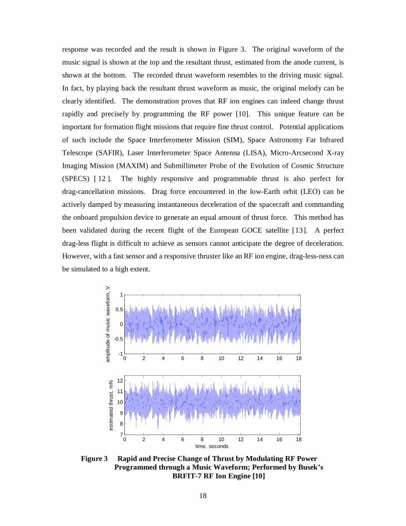
response was recorded and the result is shown in Figure 3. The original waveform of the
music signal is shown at the top and the resultant thrust, estimated from the anode current, is
shown at the bottom. The recorded thrust waveform resembles to the driving music signal.
In fact, by playing back the resultant thrust waveform as music, the original melody can be
clearly identified. The demonstration proves that RF ion engines can indeed change thrust
rapidly and precisely by programming the RF power [10]. This unique feature can be
important for formation flight missions that require fine thrust control. Potential applications
of such include the Space Interferometer Mission (SIM), Space Astronomy Far Infrared
Telescope (SAFIR), Laser Interferometer Space Antenna (LISA), Micro-Arcsecond X-ray
Imaging Mission (MAXIM) and Submillimeter Probe of the Evolution of Cosmic Structure
(SPECS) [ 12 ]. The highly responsive and programmable thrust is also perfect for
drag-cancellation missions. Drag force encountered in the low-Earth orbit (LEO) can be
actively damped by measuring instantaneous deceleration of the spacecraft and commanding
the onboard propulsion device to generate an equal amount of thrust force. This method has
been validated during the recent flight of the European GOCE satellite [13]. A perfect
drag-less flight is difficult to achieve as sensors cannot anticipate the degree of deceleration.
However, with a fast sensor and a responsive thruster like an RF ion engine, drag-less-ness can
be simulated to a high extent.
0 2 4 6 8 10 12 14 16 18-1
-0.5
0
0.5
1
ampl
itude
of m
usic
wav
efor
m, V
0 2 4 6 8 10 12 14 16 187
8
9
10
11
12
estim
ated
thru
st, m
N
time, seconds Figure 3 Rapid and Precise Change of Thrust by Modulating RF Power
Programmed through a Music Waveform; Performed by Busek’s BRFIT-7 RF Ion Engine [10]

19
1.1.3 Issues
Despite their numerous advantages, RF ion engines have not been fully accepted by the U.S.
space industry. One barrier involves the development of a highly efficient RF amplifier.
Although good efficiency is not difficult to achieve because of the low operating frequency
(order of MHz rather than GHz), problems still exist regarding scaling down the amplifier
components. Developing high-efficiency RF power electronics at smaller scales is an active
field of research but is not within the scope of this thesis.
Other issues of RF ion engines mainly concern the complex design methodology. The RF
circuit needs to be designed for high power coupling efficiency so the source does not dissipate
power within the transmission circuit. This is referred to as impedance matching and requires
the knowledge of the plasma’s electrical properties, which are not known a priori. The
selected operating frequency needs to produce the proper skin depth for RF power deposition.
Such mechanism is related to the plasma conductivity, gas pressure, chamber geometry and
coil geometry. All these parameters intertwine together and form a very complex design
problem. On top of that, parasitic power loss such as ohmic heating of the coil adds extra
design constraints as its electrical resistance could vary with temperature as well as driving
frequency.
1.2 Busek RF Ion Engines
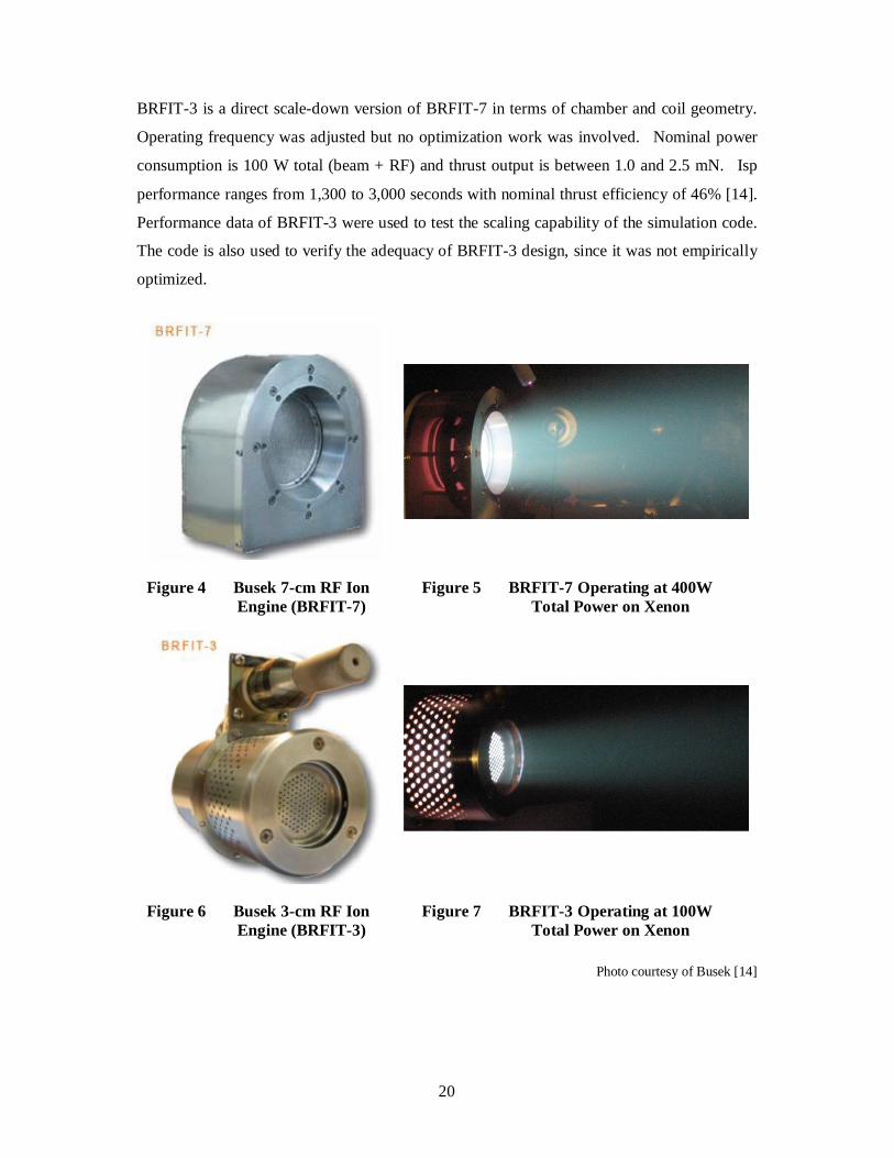
Two experimental RF ion engines developed by Busek Co., Inc. were provided for this thesis
work. Pictures of the two thrusters, designated BRFIT-7 and BRFIT-3, are shown in Figure 4
to Figure 7. Detail hardware description and critical dimensions cannot be published for
proprietary reasons. BRFIT-7, whose name stands for “Busek RF Ion Thruster” with a
7-cm-diameter grid, is throttleable between 0.7 and 14 mN thrust and can operate efficiently
over 3,300 to 5,300 sec Isp. Thrust efficiency of 75% (thrust power-to-total power ratio, not
including cathode and DC/RF conversion) can be obtained in nominal operation. Total power
consumption ranges from 150 to 400 W depending on the thrust output [14]. BRFIT-7 was
developed under the guidance of NASA/JPL and was empirically optimized to some extent.
Its performance data were used to validate the simulation code of this thesis.
20
BRFIT-3 is a direct scale-down version of BRFIT-7 in terms of chamber and coil geometry.
Operating frequency was adjusted but no optimization work was involved. Nominal power
consumption is 100 W total (beam + RF) and thrust output is between 1.0 and 2.5 mN. Isp
performance ranges from 1,300 to 3,000 seconds with nominal thrust efficiency of 46% [14].
Performance data of BRFIT-3 were used to test the scaling capability of the simulation code.
The code is also used to verify the adequacy of BRFIT-3 design, since it was not empirically
optimized.
Figure 4 Busek 7-cm RF Ion Engine (BRFIT-7)
Figure 5 BRFIT-7 Operating at 400W Total Power on Xenon
Figure 6 Busek 3-cm RF Ion Engine (BRFIT-3)
Figure 7 BRFIT-3 Operating at 100W Total Power on Xenon
Photo courtesy of Busek [14]

21
1.3 Previous Numerical Work
Experimental and theoretical work on inductively-coupled plasma (ICP) discharge has been
around for decades and is still an ongoing effort. A brief literature review is presented in this
section. This review focuses on theory development, specifically on numerical work related
to this thesis.
Inductive plasma has two distinct configurations pertaining to coil geometry. In addition to
the helical coil structure found on RF ion engines, plasma can also be generated by a planar coil
wound on one side of a discharge chamber. Planar-coil ICP has been extensively researched
in the semiconductor industry for plasma etching and surface treatment of silicon wafer. It is
seldom applied to RF ion engines as planar-coil ICPs operate at 100s of MHz frequency and the
RF power supply is not very efficient as the result. Despite different matching circuit designs,
physics on the plasma coupling mechanism are similar between the two coil types. For
general ICP discharge regardless of coil geometry, Piejak [15] developed an zero-th order
analytical model by considering the plasma discharge as a one-turn secondary of an air-core
transformer. Power deposition into the plasma was solved by finding equivalent electrical
parameters of spatially-averaged plasma properties on the primary circuit. Maxwell’s
equations were not solved using this method. Following Piejak’s work, Vahedi [16] from the
Lawrence Livermore National Laboratory constructed a more detailed analytic model to
describe power deposition in a planar-coil ICP discharge. He focused on the electromagnetic
wave interaction with the plasma, especially the spatial decay of the electric field in the “skin
effect” region. Both Piejak and Vahedi’s models show good agreement with published
experimental data and can be used for scaling the applied frequency and input power.
Higher-order computational models of ICP plasma do exist, but mostly tailored for planar-coil
type of discharge. Lymberopoulos [ 17 ], Kumar [ 18 ] and Lee [ 19 ] all developed
two-dimensional fluid simulations in which full set of Maxwell’s equations were
implemented. A two-dimension particle-in-cell/Monte Carlo (PIC/MC) model for carbon
tetrafluoride was developed recently by Takekida [20] to study selective plasma etching of
silicon oxide for manufacturing integrated circuits.
Few computational models have been developed for the plasma discharge found in RF ion
engines. Oh [21] and Froese [22] have both worked on one-dimensional versions of
PIC/MC simulations. Arzt [23] presented a two-dimensional fluid code in which ambipolar

22
diffusion, presheath potential formulation and an ion mobility term for momentum transport
are included. RF power deposition and electromagnetic field coupling were however not
described and a simple linear relationship between plasma density and RF power was used.
Mistoco [24] took a similar approach and developed a fluid model for an RF ion thruster
discharge using COMSOL multiphysics software. Mistoco’s work includes a transformer
model for calculating RF plasma dissipation. Coupling of electromagnetic field between the
coil and the plasma was again not described. Both Arzt and Mistoco’s codes assume
steady-state fluid flows and do not solve Maxwell’s equations except for the electric potential
distribution.
It is worth mentioning that Closs [25] of German Astrium GmbH (the manufacturer of RIT ion
thrusters) has developed a practical design software for RF ion engines. This software
considers many aspects of thruster operation, including thermal transfer to the thruster housing,
optimization of the coil, and ion optics. The included discharge model is however very
simplified and lacks spatial resolution. As the result the plasma discharge is not fully
characterized.
1.4 Research Objective
The objectives of this research are two-fold. The primary objective is to increase the
understanding of important aspects regarding ICP discharge. This includes how the plasma
reacts to the coil-induced electromagnetic field, electron confinement (or lack of) supplied by
the induced magnetic field, and scaling of the power deposition region that is related to the skin
effect. The second objective is to develop a systematic approach to designing and optimizing
the ICP source for an RF ion engine. Limitations of the theory should be identified and
explained if possible.
1.5 Thesis Outline
The thesis is organized in a roughly chronological order that represents how the research
progressed. Chapter 2 describes the premises of the simulation code, basic assumptions and
limitations. Chapter 3 derives the physics behind the code. It starts with a transformer model
that is used to calculate coil current and presents solution to Maxwell’s equations for

23
electromagnetic coupling between the coil and the plasma. The full set of fluid equations for
ions and electrons is detailed for momentum and particle transport. The system is closed by
equations of global energy balance and global neutral particle balance. Chapter 4 presents
simulation results and comparisons with a benchmark thruster, the Busek thruster BRFIT-7.
Comparison with the BRFIT-3 is also conducted to demonstrate scaling capability of the code.
A brief optimization study for the BRFIT-3 is presented at the end of Chapter 4. Finally,
Chapter 5 summarizes the accomplishments and contributions of this research, and
recommends future work.
24
Chapter 2
MODEL DESCRIPTION
A two-dimensional simulation is developed for the ICP discharge inside an RF ion engine.
Both electrons and singly-charged ions are treated as fluid continuum and neutral atoms are
assumed as stationary background. Quasi-neutrality is imposed throughout the discharge.
Differential forms of Maxwell’s equations are solved along with full sets of fluid equations. A
time-domain approach is used to resolve the electromagnetic wave propagation and plasma
current induction. Ion momentum is also solved with time dependency to allow plasma to
reach its potential and density distribution in steady-state. The code considers cylindrical
coordinates with 2D in space (vr, vz) and 3D in velocity (vr, vθ, vz). Xenon is the default
propellant but other gases can be easily adopted by incorporating the necessary cross section
data.
A previously-developed transformer model is implemented for finding the coil current that
serves as discharge source. It takes spatially-averaged plasma properties and calculates their
equivalent impedance in the primary circuit. By prescribing RF forward power, source
impedance (typically 50 Ω) and circuit capacitance, the model can approximate the amount of
current passing through the RF coil. Since the plasma properties change over time, this
transformer sub-model is accessed at every time step for finding the coil current. The
time-dependent coil current is used to compute the coil-induced magnetic field, which can be
coupled to the plasma current through solution of Maxwell’s equations.
The code is written in serial form and executed in MATLAB, a software package developed by
MathWorks, Inc. The MATLAB language is very similar to C++ and the software can be
complied on any PC or work station. Convergence is determined by cyclic steady-state
observation of anode current, electron temperature, and various dissipated powers.
Convergence time using a 4 GHz, 64-bit processor and 4 GB memory is approximately two
hours.

25
2.1 Fluid Approximation
Modeling charged particles as fluid in a high-frequency plasma discharge has been widely
accepted. This assumption is valid for pressures >100 mTorr where collisions dominate
[18,26]. RF ion engines however operate at much lower pressure, typically 1-10 mTorr, so
verification is needed before applying this assumption. Mikellides [27] suggests the onset of
collisional plasma occurs when the mean-free-path of charged particle is significantly less than
the characteristic length of the discharge vessel. He uses the following inequality to justify the
fluid assumption, which can be adopted for general use.
4.0L
Kn mfp ( 1 )
where Kn is the Knudsen number defined as the ratio between mean-free-path λmfp and
characteristic length L. Although in an RF ion engine the Knudsen number for electrons can
be high, it is less meaningful because electrons can be repelled by the sheath potential which
increases their chance for collision. Ions, on the other hand, have no confinement mechanism
and speed toward the walls. So the ion-neutral collision is the important issue here concerning
the validity of the continuum assumption. The mean-free-path for ion-neutral collision is
defined as
inn
mfp Qn1
( 2 )
where nn is the neutral number density and Qin is the ion-neutral scattering cross section
modeled from Banks’ formula [28],
r
in cQ
161028072.8 , [m2] ( 3 )
The denominator term iir mkTc 16 is the relative thermal velocity between
singly-charged ions and background neutrals and is defined with reduced mass. The neutral
number density can be approximated by a Maxwellian-averaged flux equation for neutral flow,
26
ngridnn
n Acnmm 4
( 4 )
with iin mkTc 8 being the mean thermal velocity of neutrals, Agrid the grid area and φn
the effective grid transparency to the neutrals. The grid transparency to neutrals is difficult to
define because there is a slight confinement from the geometry of the grid aperture. However, a
first-order estimation can be reached for a two-grid system,
1111
accelscreenn
( 5 )
where φscreen and φaccel represent the physical opening of screen grid and accelerator grid
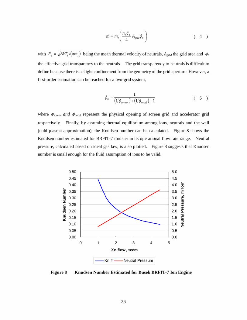
respectively. Finally, by assuming thermal equilibrium among ions, neutrals and the wall
(cold plasma approximation), the Knudsen number can be calculated. Figure 8 shows the
Knudsen number estimated for BRFIT-7 thruster in its operational flow rate range. Neutral
pressure, calculated based on ideal gas law, is also plotted. Figure 8 suggests that Knudsen
number is small enough for the fluid assumption of ions to be valid.
0.000.05
0.100.15
0.200.25
0.300.35
0.400.45
0.50
0 1 2 3 4 5
Xe flow, sccm
Knud
sen
Num
ber
0.00.5
1.01.5
2.02.5
3.03.5
4.04.5
5.0
Neut
ral P
ress
ure,
mTo
rr
Kn # Neutral Pressure
Figure 8 Knudsen Number Estimated for Busek BRFIT-7 Ion Engine
27
2.2 Basic Assumptions
The requirement for a self-sustaining plasma is that sufficient ionization must take place to
compensate for wall losses. Though time-dependency is considered, this code does not model
transient effects and must be started with sufficient amount of plasma density to overcome the
immediate ion fluxes to the walls. The code also considers the case of pure ICP discharge and
cannot handle capacitively-coupled plasma (CCP) discharges. Models with such combining
effect, also known as E-H mode transition, can be found in Ref. 29. Other mathematical and
physical assumptions are enumerated below for clarity. They are generally accepted for
modeling inductively-coupled plasmas with heavy noble gas.
1) In cylindrical axis-symmetry, all quantities are functions of coordinates r and z (except for
a globally-defined value), but independent of θ. Symmetry condition also requires 0
throughout the computational domain and 0 r at the axis of symmetry.
2) The plasma contains electrons, singly-charged ions and neutrals in quantities ne, ni, and nn.
Quasi-neutrality is imposed throughout the plasma so ni = ne. Due to low ionization
percentage in an RF ion engine, neutrals are assumed as stationary background. Neutral
density nn is therefore a global variable, but time-dependent. Charge-exchange between ions
and neutrals is not accounted for.
3) The electrons are assumed to be in thermal equilibrium at a volume averaged value Te.
The ions are near equilibrium with the neutrals at a significantly lower temperature such that
Ti ~ Tn << Te. Ions and neutral particles are then given a temperature close to the wall
temperature, estimated as 450 K from experimental observation. The effect of wall
temperatures between 400 and 600 K was explored and the changes in simulation results are
miniscule.
4) Because electrons possess higher thermal velocity than ions, they rush out of the plasma
toward the walls and leave behind excess of positive charge behind. The resulting positive
charge density gives rise to an electrostatic field that repels the electrons and accelerates the
ions [23]. This is referred to as pre-sheath region where space-charge field links together the
trajectory of electrons and ions such that ambipolar diffusion can be assumed. In the code,
ambipolar diffusion is carried out to the boundary, where the ions reach sonic speed and the
Bohm criterion is satisfied. Ions that reach this boundary are eventually returned to the

28
plasma as neutrals for mimicking wall recombination. The plasma sheath, which is a thin
layer in front of the walls where the ion density is much greater than the electron density, is not
resolved.
5) Azimuthal ion current is negligible as the induced plasma current is mainly contributed by
the fast-moving electrons. The direction of the induced electric field is alternating at such
high frequency (order of MHz) that the heavy ions do not have sufficient time to react to it.
The azimuthally induced electron current is assumed dominant over meridional-plane (r-z
plane) electron diffusion currents. This assumption is based on the ICP working mechanism.
As such, meridional-plane electron currents do not contribute to magnetic field generation and
coupling.
6) The helical coil is approximated as separate rings of concentrated current source. This
allows completion of the 2D axisymmetric assumption. The validity of this claim is examined
in the next section. Electrical resistance of the coil is a required input for the code for
estimating ohmic loss and is assumed constant regardless of the operating condition.
7) The plasma discharge is treated as a “black box” in the sense that the influence of the
extraction system on the source plasma is neglected. The model however employs a known
ion transparency function of the grids for a specific operating condition. The ion transparency
is used to calculate the extractable ion beam current given the ion flux arriving to the screen
grid. This is only meant for benchmarking the code against a measurable quantity and is not
intended for broader purpose. The physics of ion optics and the computation of ion
trajectories can be found in Ref. 30
2.3 The Spatial 2D Assumption For the model to consider only 2D in space, rather than 3D, it requires the assumption of an
axisymmetric RF coil. Under such assumption, the coil generates electric field purely in the
azimuthal (θ) direction and magnetic field purely in the radial and axial (r and z) directions.
The plasma current is subsequently induced only in the θ direction. By neglecting magnetic
contributions from the diffusion current in the meridional plane, the plasma-induced magnetic
field becomes significant only in r and z directions. The spatial 2D assumption then holds true
for magnetic field coupling between the plasma and the coil.
29
Such assumption is generally adequate because the cylindrical discharge chamber found in an
RF ion engine is usually short axially for the purpose of minimizing wall loss, which renders a
short coil with its winding diameter being longer than its axial length. This configuration
naturally suggests axis-symmetry from the geometrical point of view. In fact, over the years
many studies on ICP discharge have adopted 2D axisymmetric approach for various coil
geometries [31].
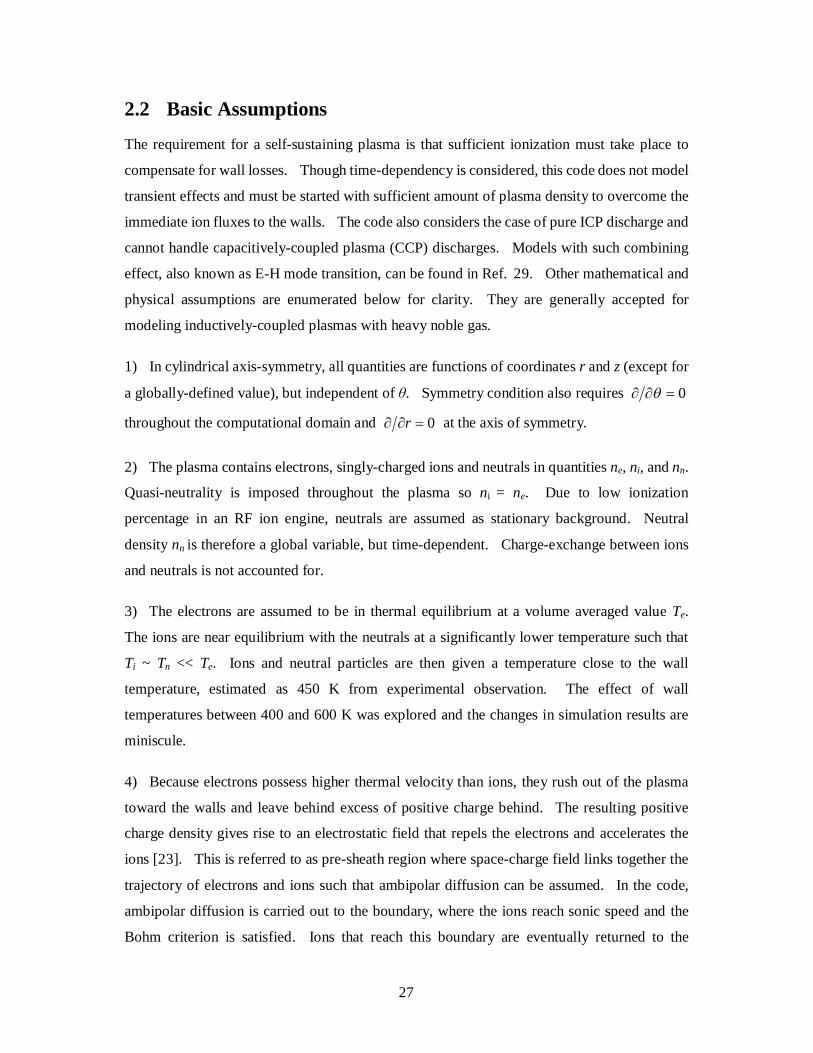
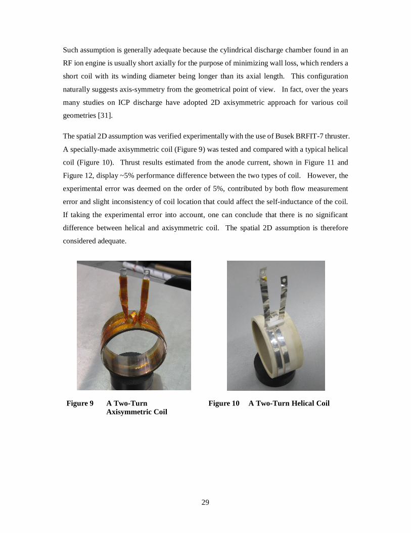
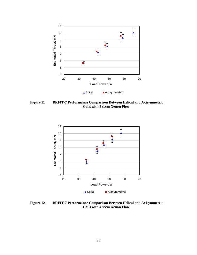
The spatial 2D assumption was verified experimentally with the use of Busek BRFIT-7 thruster.
A specially-made axisymmetric coil (Figure 9) was tested and compared with a typical helical
coil (Figure 10). Thrust results estimated from the anode current, shown in Figure 11 and
Figure 12, display ~5% performance difference between the two types of coil. However, the
experimental error was deemed on the order of 5%, contributed by both flow measurement
error and slight inconsistency of coil location that could affect the self-inductance of the coil.
If taking the experimental error into account, one can conclude that there is no significant
difference between helical and axisymmetric coil. The spatial 2D assumption is therefore
considered adequate.
Figure 9 A Two-Turn Axisymmetric Coil
Figure 10 A Two-Turn Helical Coil
30
4
5
6
7
8
9
10
11
20 30 40 50 60 70
Load Power, W
Estim
ated
Thr
ust,
mN
Spiral Axisymmetric
Figure 11 BRFIT-7 Performance Comparison Between Helical and Axisymmetric
Coils with 3 sccm Xenon Flow
4
5
6
7
8
9
10
11
20 30 40 50 60 70
Load Power, W
Est
imat
ed T
hrus
t, m
N
Spiral Axisymmetric
Figure 12 BRFIT-7 Performance Comparison Between Helical and Axisymmetric
Coils with 4 sccm Xenon Flow
31
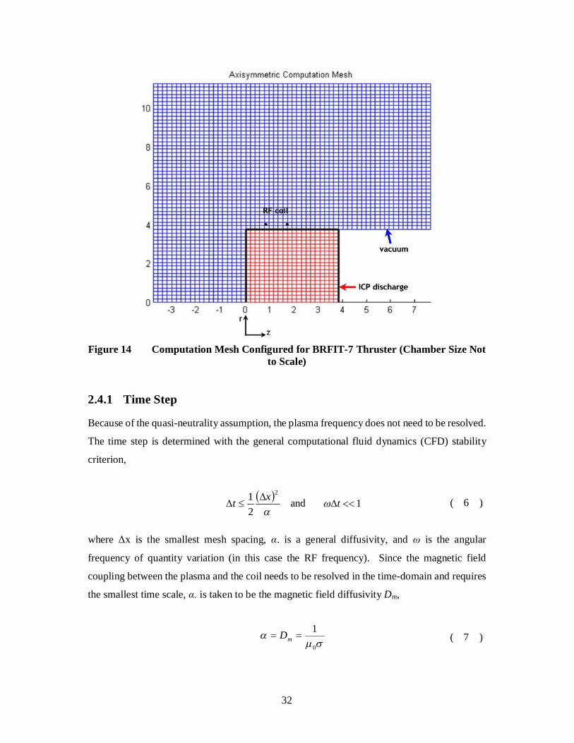
2.3 Computation Domain 2.4.1 Mesh
The main plasma code takes a computational fluid dynamics (CFD) approach with the addition
of Maxwell’s equations. A finite-difference algorithm with 2nd order accuracy differencing
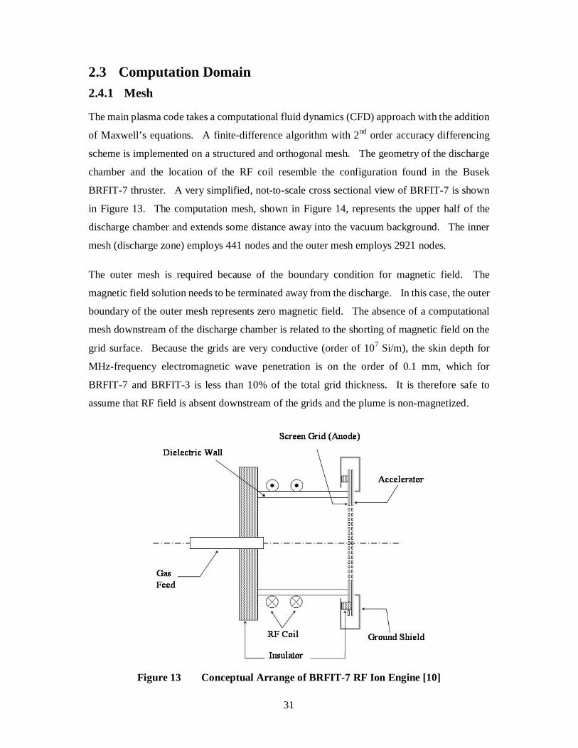
scheme is implemented on a structured and orthogonal mesh. The geometry of the discharge
chamber and the location of the RF coil resemble the configuration found in the Busek
BRFIT-7 thruster. A very simplified, not-to-scale cross sectional view of BRFIT-7 is shown
in Figure 13. The computation mesh, shown in Figure 14, represents the upper half of the
discharge chamber and extends some distance away into the vacuum background. The inner
mesh (discharge zone) employs 441 nodes and the outer mesh employs 2921 nodes.
The outer mesh is required because of the boundary condition for magnetic field. The
magnetic field solution needs to be terminated away from the discharge. In this case, the outer
boundary of the outer mesh represents zero magnetic field. The absence of a computational
mesh downstream of the discharge chamber is related to the shorting of magnetic field on the
grid surface. Because the grids are very conductive (order of 107 Si/m), the skin depth for
MHz-frequency electromagnetic wave penetration is on the order of 0.1 mm, which for
BRFIT-7 and BRFIT-3 is less than 10% of the total grid thickness. It is therefore safe to
assume that RF field is absent downstream of the grids and the plume is non-magnetized.
Figure 13 Conceptual Arrange of BRFIT-7 RF Ion Engine [10]
32
Figure 14 Computation Mesh Configured for BRFIT-7 Thruster (Chamber Size Not
to Scale)
2.4.1 Time Step
Because of the quasi-neutrality assumption, the plasma frequency does not need to be resolved.
The time step is determined with the general computational fluid dynamics (CFD) stability
criterion,
2
21 xt
and 1t ( 6 )
where Δx is the smallest mesh spacing, α. is a general diffusivity, and ω is the angular
frequency of quantity variation (in this case the RF frequency). Since the magnetic field
coupling between the plasma and the coil needs to be resolved in the time-domain and requires
the smallest time scale, α. is taken to be the magnetic field diffusivity Dm,
0
1 mD ( 7 )

33
where µ0 is the permeability of free space and σ is the plasma conductivity. From
post-examining simulation results is found to be 500-1000 Si/m under various operating
conditions of BRFIT-7. Given the thruster geometry and the computational mesh used, the
maximum allowable t is approximately 10-9 seconds. In the code, t is found by
prescribing the number of points that each wave period is resolved,
resolutionN
ft /1 ( 8 )
where f is the driving frequency in hertz and Nresolution is the number of points discretizing the
RF wave in time. The default Nresolution is 2000, rendering a t on the order of 10-10 seconds.
34
Chapter 3
THEORY
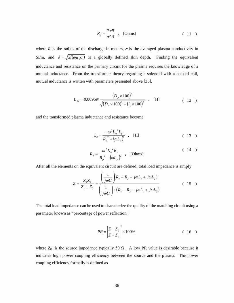
The theory section is divided into four major parts. Section 3.1 presents a transformer model
that is used to calculate the RF coil current. Section 3.2 is the main ICP discharge model,
which includes the physics of inductive coupling, plasma current generation, formulation of
plasma conductivity and a fluid model that addresses the diffusion of charged particles.
Following the discharge model is a description of the numerical method in Section 3.3. This
section details the computation of the coil-induced magnetic field and contains important
boundary conditions and the finite-difference CFD scheme. Lastly, a simple ion optics model
is presented for the purpose of benchmarking the code with measured experimental data. The
ion optics model is case-specific and is not intended for general use.
3.1 Transformer Model Using a transformer analogy to calculate circuit properties of an RF plasma is not new. Many
people have developed similar models as presented in Ref. 15, 24 and 32. While such a
zero-th order model is typically used to estimate the power dissipated by the plasma, it is
employed in the code only for finding the coil current. This model is needed because
prescribing the external loop current or loop potential for an ICP discharge simulation is not an
intuitive method. Often these quantities are not known to the user and therefore do not serve
well as inputs for the discharge simulation.
The transformer model used in the code is based on previous work described in Ref. 32. The
basic idea is to model the whole RF circuit as a transformer with the plasma being a one-turn
secondary coil. Figure 15 illustrates the premise. The circuit representation shown in Figure
15 is known as a parallel matching circuit since the capacitive element is placed in parallel to
the plasma load. After all equivalent circuit parameters are defined by the transformer model,
total load impedance is calculated and with it the coil current is found.
35
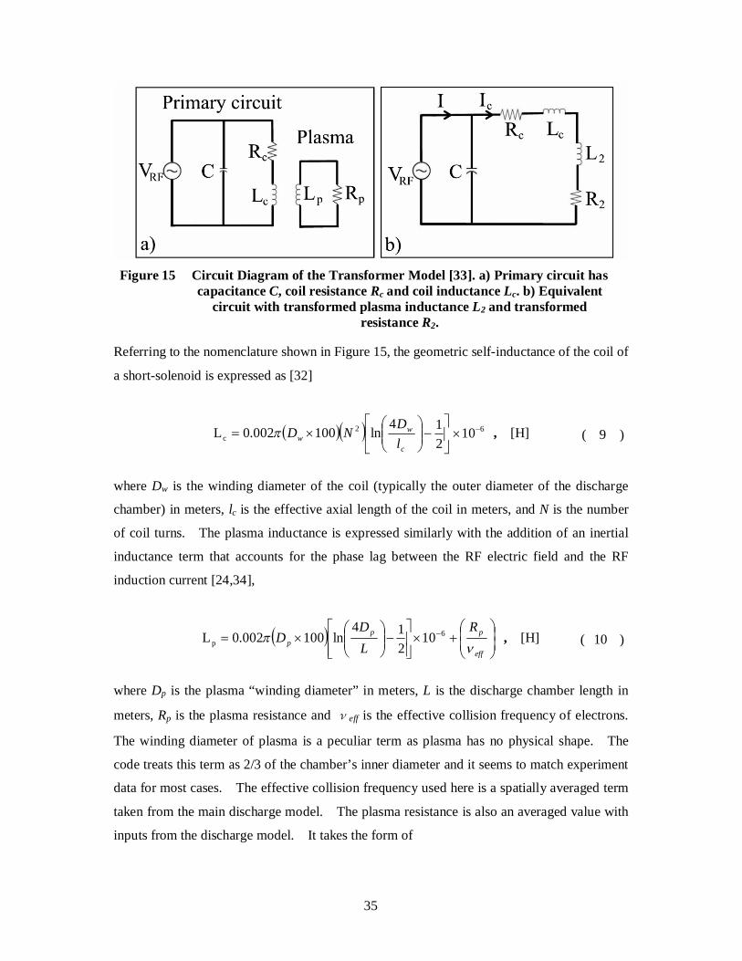
Figure 15 Circuit Diagram of the Transformer Model [33]. a) Primary circuit has
capacitance C, coil resistance Rc and coil inductance Lc. b) Equivalent circuit with transformed plasma inductance L2 and transformed
resistance R2.
Referring to the nomenclature shown in Figure 15, the geometric self-inductance of the coil of
a short-solenoid is expressed as [32]
214
ln100002.0L 2c
c
ww l
DND 610 , [H] ( 9 )
where Dw is the winding diameter of the coil (typically the outer diameter of the discharge
chamber) in meters, lc is the effective axial length of the coil in meters, and N is the number
of coil turns. The plasma inductance is expressed similarly with the addition of an inertial
inductance term that accounts for the phase lag between the RF electric field and the RF
induction current [24,34],
eff
ppp
RLD
D
6p 10
214
ln100002.0L , [H] ( 10 )
where Dp is the plasma “winding diameter” in meters, L is the discharge chamber length in
meters, Rp is the plasma resistance and νeff is the effective collision frequency of electrons.
The winding diameter of plasma is a peculiar term as plasma has no physical shape. The
code treats this term as 2/3 of the chamber’s inner diameter and it seems to match experiment
data for most cases. The effective collision frequency used here is a spatially averaged term
taken from the main discharge model. The plasma resistance is also an averaged value with
inputs from the discharge model. It takes the form of
36
L
RRp2
, [Ohms] ( 11 )
where R is the radius of the discharge in meters, σ is the averaged plasma conductivity in
Si/m, and 02 is a globally defined skin depth. Finding the equivalent
inductance and resistance on the primary circuit for the plasma requires the knowledge of a
mutual inductance. From the transformer theory regarding a solenoid with a coaxial coil,
mutual inductance is written with parameters presented above [35],
22
2
m100100
1000095.0L
cw
p
lD
DN , [H] ( 12 )
and the transformed plasma inductance and resistance become
22
22
2pp
pm
LRLL
L
, [H] ( 13 )
22
22
2pp
pm
LRRL
R
, [Ohms]
( 14 )
After all the elements on the equivalent circuit are defined, total load impedance is simply
22
22
21
21
1
1
LjLjRRCj
LjLjRRCj
ZZZZZ
cc
cc
( 15 )
The total load impedance can be used to characterize the quality of the matching circuit using a
parameter known as “percentage of power reflection,”
%1002
0
0
ZZZZPR ( 16 )
where Z0 is the source impedance typically 50 Ω. A low PR value is desirable because it
indicates high power coupling efficiency between the source and the plasma. The power
coupling efficiency formally is defined as

37
Power Couple Efficiency = 1 – Power Reflection % ( 17 )
The load impedance parameter from Eq. 15, more importantly, is used to calculate the peak
current drawn from the source,
0
0
0
0 12
ZZZZ
ZPZ
I forwardpeak ( 18 )
which leads to the RMS coil current using current divider law,
221
1,
ZZ
ZII peakRMScoil ( 19 )
Note that the coil current is actually treated as a sine wave in the main discharge code. The
RMS coil current found here is utilized to change the amplitude of that sinusoidal function at
each time step, which subsequently excites the discharge. This method takes into account the
interaction among plasma, RF coil and power source without having to solve the backward EM
wave induced on the primary circuit by the plasma.
3.2 ICP Discharge Model
The discharge model is presented first with solutions to Maxwell’s equations, followed by
formulations of plasma parameters that are unique for ICP discharge and the fluid equations
describing charged particle diffusion. Diffusion of plasma is considered up to the sheath edge
with ions reaching sonic speed at the computational boundary. The plasma sheath is not
resolved by this code. The discharge model concludes with equations regarding the neutral
particle conservation and the electron power balance within the discharge. Xenon plasma is
considered and its cross section data are default in the code.
3.2.1 Magnetic Field Coupling and Plasma Current Induction
Magnetic field coupling is a natural phenomenon in ICP discharge that occurs when the
coil-induced magnetic field is distorted from the induction of plasma current. Physics of this
coupling effect can be realized by solving Maxwell’s equations of electromagnetism. Eq.
38
20-23 show the full set of Maxwell’s equations assuming the magneto-quasi-static (MQS)
condition which neglects the displacement current. This is generally valid for low MHz
frequency.
tBE
( 20 )
jB
0
( 21 )
0 B
( 22 )
0
chE
( 23 )
Because quasi-neutral plasma is assumed, the electric potential is solved from fluid equations
rather than from charge distribution and Eq. 23 is no longer needed. In the model, the
solution for the magnetic field is represented by the magnetic vector potential A
; it is defined
as,
AB
and 0 A
( 24 )
From the definition of A
, Eq. 22 is automatically satisfied. As explained in Section 2.2
regarding the spatial 2D assumption, the magnetic fields considered here are only Br and Bz,
which means that only the θ component of the vector potential exists. Thus, the Coulomb
gauge condition ( 0 A
) is also automatically satisfied,
01
z
AArr
Ar
AA zrr
( 25 )
because the first, second and fourth term drops out, and the ∂/∂θ term is zero due to
axis-symmetry. Since 0 A
is valid, the following vector property holds true,
AAAA
22 ( 26 )
39
Faraday’s law represented by Eq. 20 can be written with the use of A
,
tAA
ttBE
0
tAE
( 27 )
from which a scalar electric potential φ can be defined,
tAE
tAE
( 28 )
By combining Eq. 21 and the derived properties of A
field, the equation governing the
induced plasma current with respect to the magnetic vector potential is reached,
jB
0
jA
0 jA
02 ( 29 )
Because the induced ion current is neglected (Section 2.2), the current density term in Eq. 29 is
purely an electron current and is modeled as
e
ee en
PEjj
( 30 )
where eP is the electron pressure gradient representing body force and σ is the plasma
conductivity that will be derived in the next section. The electron pressure gradient is
expressed with the assumption of ideal gas and constant electron temperature, so that
eee nkTP ( 31 )
Now substituting Eq. 30 and Eq. 28 into Eq. 29, the following equation is obtained,
e
e
e
e
enP
tA
enPEA
002 ( 32 )
From the spatial 2D assumption, the A field retains only the θ component. Eq. 32 therefore
considers solely the θ component of the partial derivatives. The gradient terms regarding

40
electric potential and electron pressure Pe are immediately dropped because of
axis-symmetry. The only terms left are
t
ArAA
022 ( 33 )
Since both the coil and the plasma contribute to the induced Aθ, it is considered a superposition
of these two contributions
plco AAA ( 34 )
where the subscripts “co” and “pl” denote coil and plasma respectively. Substituting the above
expression into Eq. 33 and rearranging, Eq. 35 is obtained as following,
t
At
Ar
AAr
AA coplco
copl
pl
002
22
2 ( 35 )
The large bracket on the right-hand-side of Eq. 35 refers to the vector Laplacian of the
coil-induced A field in the direction, and its value should be zero. This can be verified by
taking an example of time-invariant coil current that generates a coA field but
0 tA co (a DC field). Because there is no electromagnetic wave, no plasma current is
induced and subsequent no plA would exist. Eq. 35 in this example would have zeros all
across except for the large bracket, which must equal to zero as the result. With this
realization, Eq. 35 is reduced to the final form for governing magnetic field diffusion,
source
coplplpl t
At
Ar
AA 02
2 ( 36 )
Eq. 36 is an important result because it shows that although the coil field and the plasma field
are physically coupled, the coil field can be treated as a decoupled source term in this diffusion
equation. By pre-computing the coil-induced source field (Aθ)co in the background with
respect to space and time, (Aθ)pl field can be computed everywhere at each time step. More
41
importantly, once the total field Aθ is found, the azimuthally-induced plasma current can be
calculated from the combined form of Eq. 33 and Eq. 29,
j
tA
rAA 002
2
t
Aj ( 37 )
The importance of this Eq. 37 is twofold. First, it describes the induction of azimuthal plasma
current in the presence of a propagating magnetic field. This plasma current dissipates power
into the plasma through local ohmic heating, which is the working mechanism of ICP discharge.
The azimuthal plasma current is also required to compute the ionization and excitation rate
because electrons are modeled by a shifted Maxwellian energy distribution function with drift
energy in the azimuthal direction.
3.2.2 Plasma Conductivity
Plasma conductivity in the discharge model is considered a local quantity and is derived with a
classical approach. Consider a non-magnetized uniform plasma in the presence of a
background gas that is driven by a time-varying electric field with frequency ω,
tjxx eEtE Re
( 38 )
where Ex is the electric field amplitude. Motion of ions is neglected by assuming an infinite
mass. Take a 1D approach and assume the electrons accelerate along the electric field with
impedance from collisionality. The equation of motion for electrons is
xeffx
x umEedtudm
( 39 )
where νelastic is the scattering frequency that contains electron-neutral and electron-ion elastic
collision. Letting the electron velocity oscillate with the same frequency,
tjxx eutu Re
( 40 )
and using the expression along with Eq. 38 and Eq. 39, the velocity is obtained with a
complex amplitude,
42
xelasticxx uEmeju x
elasticx E
jmeu
( 41 )
Since the plasma current, under the absence of ion contribution, is written as
exe neuj ( 42 )
Eq. 41 can be substituted in to obtain
x
elastic
ee E
jmnej
2
( 43 )
The conductivity term can therefore be defined in the complex sense as
jm
ne
celasti
e2
Re with enneeiieeneielastic QncQnc ( 44 )
where νei is the Coulomb collision frequency, νen is the electron-neutral scattering frequency,
and the mean velocity is the thermal velocity of electrons eee mkTc 8 . An effective
collision frequency for electrons can be defined for Eq. 44 in complex notation,
jcelastieff ( 45 )
The Coulomb collision in low-pressure ICP discharge is not as significant because ionization
fraction is typically less than 5% and electrons are less likely to interact with ions than neutrals.
Nevertheless the Coulomb term is included in the model. The Coulomb cross section is
modeled numerically [36],
eVTT
eQee
ei ,ln1087.2
4ln
94 14
20
4
[cm2] ( 46 )
with the Coulomb logarithm approximated as

43
3313
230 ,log5.0,log5.157.13
42
3lnln
cmneVT
neT
eee
e
( 47 )
The energy-averaged electron-neutral scattering cross section Qen is discussed in the next
section.
3.2.3 Energy-Averaged Cross Sections
The cross sections for electron-neutral scattering, single ionization and excitation are averaged
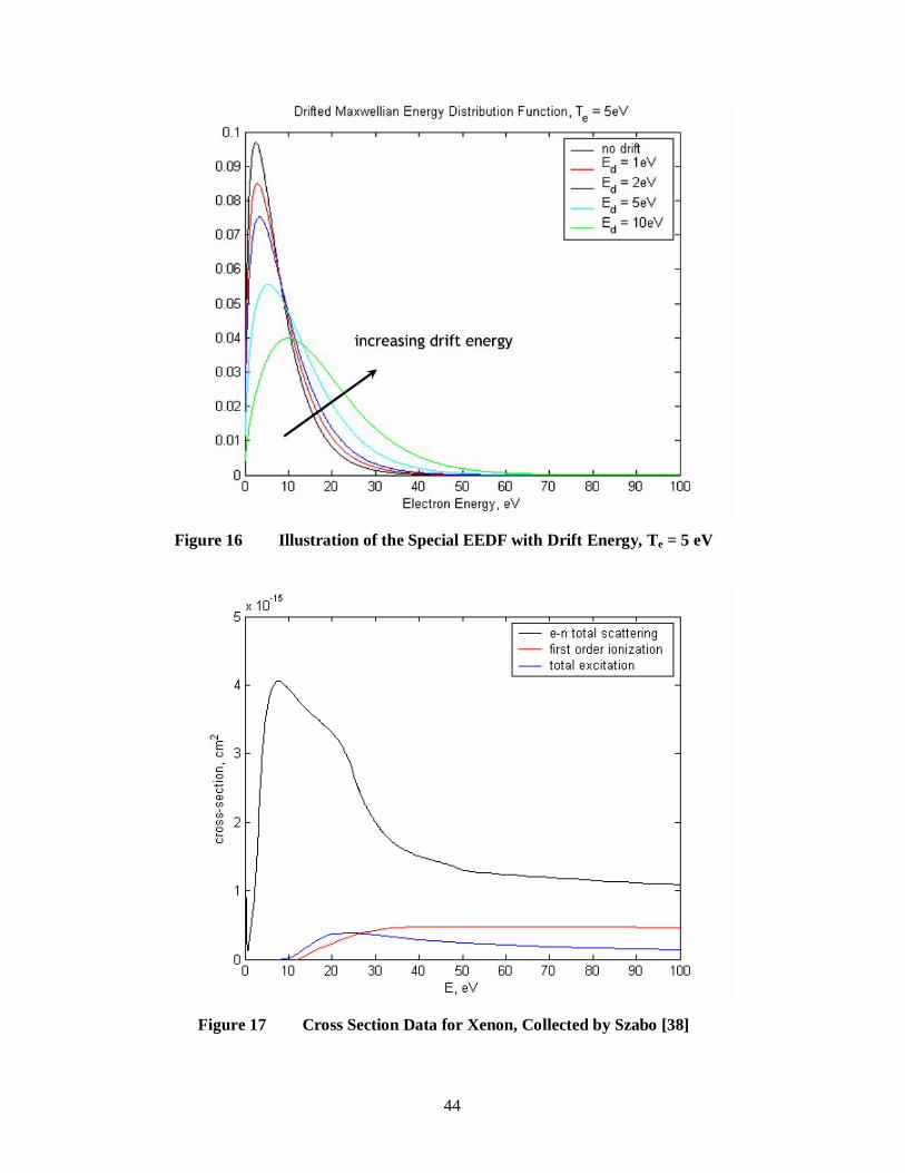
in the energy space with a special electron energy distribution function (EEDF) that considers a
drift energy ED in the direction of electric field [37],
e
D
e
D
kTEE
kTEE
DeDeD ee
EkTEETf
4
12
1),,(
2
( 48 )
The special EEDF, graphically illustrated in Figure 16 for the case of 5 eV electron temperature,
is derived from the zero-th spherical harmonic of a shifted Maxwellian EEDF in the velocity
space,
e
Dzre
kTvwwwm
e
eDeD e
kTmwvTf 2
23 222
2),,(
( 49 )
where w is the velocity-space vector and vD is the drift velocity in the azimuthal direction.
This derivation can be found in Appendix A. The method of decomposing a non-symmetric
distribution function (Eq. 49) into its zero-th spherical harmonic is valid here because cross
sections are always spherically symmetric and proportional to only the zero-th harmonic.
Thus for averaging purposes all the higher harmonics of the distribution function cancel out as
they are defined to be orthogonal to each other.
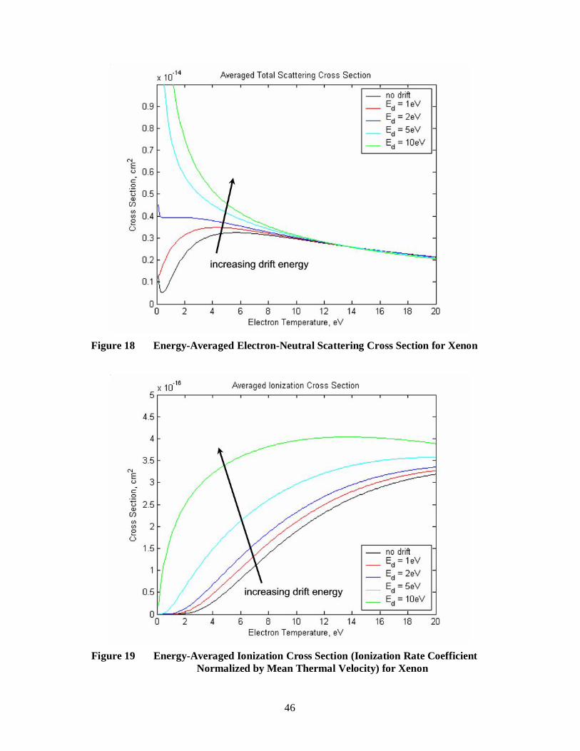
The cross section data were obtained from Szabo’s collection and curve fits shown in Ref. 38.
They are presented in Figure 17. Tabulated form of ionization and excitation cross sections
can be found in Appendix B and Appendix C. First ionization energy and first excitation
energy for xenon are 12.1 eV and 8.32 eV respectively. The data of excitation cross section
used here does not differentiate levels of excitation and lumped-sum estimation is used.
44
Figure 16 Illustration of the Special EEDF with Drift Energy, Te = 5 eV
Figure 17 Cross Section Data for Xenon, Collected by Szabo [38]

45
The cross sections are averaged in the energy space with the special EEDF (Eq. 48),
e
DeDDe c
dEEQEETfcETQ
),,(
, ( 50 )
where ec is approximated by the electron mean thermal velocity and Q is a type of cross
section. Notice that if Q represents ionization or excitation, Q is actually the rate coefficient
normalized by the electron mean thermal velocity. This normalization is for visual illustration
only and does not affect the averaging results because in the code the same mean thermal
velocity is multiplied back to obtain the originally computed rate coefficients. Since the
EEDF depends both on the drift energy and electron temperature, no analytical expression can
be found for Eq. 50 and numerical integration is required. The code pre-computes and stores
these values in a 3D form with respect to Te, ED, and averaged cross sections. The numerical
integration takes the form
n
j e
jDej
eDe E
mE
EQETEfc
ETQ1
2),,(1, ( 51 )
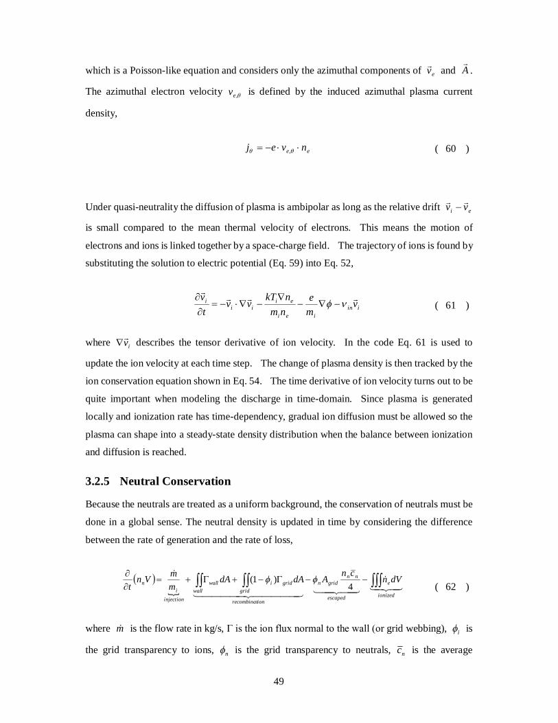
where the energy is averaged up to 100 eV. Results of the numerical integration are shown in
Figure 18 to Figure 20. The range of drift energy considered here is sufficient for
low-pressure ICP discharge. In fact, post-examining the simulation results reveals that the
drift energy does not exceed 2 eV.
46
Figure 18 Energy-Averaged Electron-Neutral Scattering Cross Section for Xenon
Figure 19 Energy-Averaged Ionization Cross Section (Ionization Rate Coefficient
Normalized by Mean Thermal Velocity) for Xenon

47
Figure 20 Energy-Averaged Excitation Cross Section (Excitation Rate Coefficient
Normalized by Mean Thermal Velocity) for Xenon
3.2.4 Fluid Equations
The governing equations for plasma diffusion in the meridional plane are derived from a
two-fluid isentropic Euler-Poisson system [39]. Magnetic force on the electron is also
considered in the momentum equation:
iiniiiiii
iii vnmEenPvv
tvnm
( 52 )
eeffeeeeeeee
eee vnmBvenEenPvv
tv
nm
, ( 53 )
iiii nvn
tn
( 54 )
eeee nvnt
n
( 55 )
where n is the rate of ionization in terms of particle density. The effective elastic collision
frequency for electrons νeff is previously defined in Eq. 36 and the ion-neutral scattering

48
frequency νin can be calculated from the cross section model presented in Eq. 3.
Recombination is treated by a global neutral particle balance, which is discussed in the next
section.
The electron inertial terms are neglected in Eq. 53 to result in a drift-diffusion approximation
for the electron flux,
BvtAnnDvn eeeeeeee
( 56 )
where effe
ee m
kTD
is the electron diffusivity and e
ee kT
eD is the electron mobility. The
A
field actually does not have r and z components because of the axis-symmetric argument so
it does not contribute to the electron flux in the meridional plane.
A quasi-neutral condition is introduced to the fluid equations so the computation domain does
not need to resolve the Debye length and the plasma frequency. The quasi-neutrality
constraint ni = ne can be expressed by taking the difference of the continuity equations (54) and
(55) and leads to the divergence-free constraint of current,
0 eeie vnvnj ( 57 )
Since 0 , Eq. 57 also implies that divergence of current in the meridional plane is zero.
Eq. 57 is used to find the electric potential in the absence of Poisson’s equation. This is done
by substituting in Eq. 56 and rearranging,
0
Bv
men
nmPn
menvn e
effe
e
effee
ee
effe
eie
( 58 )
Multiply electron charge e across and substitute in the expressions for plasma conductivity,
electron pressure (from ideal gas law) and magnetic vector potential to obtain the governing
equation of electric potential,
Avn
mekTvne ee
effe
eie
( 59 )
49
which is a Poisson-like equation and considers only the azimuthal components of ev and A
.
The azimuthal electron velocity ,ev is defined by the induced azimuthal plasma current
density,
ee nvej , ( 60 )
Under quasi-neutrality the diffusion of plasma is ambipolar as long as the relative drift ei vv
is small compared to the mean thermal velocity of electrons. This means the motion of
electrons and ions is linked together by a space-charge field. The trajectory of ions is found by
substituting the solution to electric potential (Eq. 59) into Eq. 52,
iin
iei
eiii
i vme
nmnkTvv
tv
( 61 )
where iv describes the tensor derivative of ion velocity. In the code Eq. 61 is used to
update the ion velocity at each time step. The change of plasma density is then tracked by the
ion conservation equation shown in Eq. 54. The time derivative of ion velocity turns out to be
quite important when modeling the discharge in time-domain. Since plasma is generated
locally and ionization rate has time-dependency, gradual ion diffusion must be allowed so the
plasma can shape into a steady-state density distribution when the balance between ionization
and diffusion is reached.
3.2.5 Neutral Conservation
Because the neutrals are treated as a uniform background, the conservation of neutrals must be
done in a global sense. The neutral density is updated in time by considering the difference
between the rate of generation and the rate of loss,
ionized
e
escaped
nngridn
ionrecombinat
gridgridi
wallwall
injectioni
n dVncn
AdAdAmmVn
t
4)1(
( 62 )
where m is the flow rate in kg/s, Γ is the ion flux normal to the wall (or grid webbing), i is
the grid transparency to ions, n is the grid transparency to neutrals, nc is the average

50
thermal velocity of the neutrals, and wallA and gridA are the wall and grid areas. On the
right-hand-side of Eq. 62, the first term describes flow injection rate into the chamber, the
second term describes the neutrals being introduced back to the chamber after ions recombined
at the wall, the third term describes the rate of neutrals escaping through grid apertures, and the
fourth term describes the consumption of neutrals due to ionization.
3.2.6 Discharge Energy Balance
The electron temperature is taken to be a spatially-averaged value in the discharge model. The
energy balance for electrons therefore must be considered on a global scale. The governing
equation is formulated by tracking the averaged change of internal energy in the discharge.
The change of internal energy is the difference between the power absorbed by the plasma and
the energy expended within. Absorbed power, or power dissipated into the discharge, is
contributed mainly by the induced current ,ej through ohmic heating. Power dissipation by
the meridional-plane electron current is ignored. Energy expenditure within the discharge
consists of ionization, excitation, and kinetic energy loss in the sheath and to the walls. The
energy balance model is presented in Eq. 63. Previous investigation concluded that the energy
loss due to Coulomb collision is negligible and it is therefore not included.
losssheathwall
wallwallsheathe
excitation
excexc
ionization
ie
ndissipatio
eee
dAekT
dVeVndVeVndVj
dVnkTt
2
23 2
,
( 63 )
In Eq. 63, ,ej is the azimuthal electron current, wall is the electron flux normal to the walls,
en is the ionization rate with Vi = 12.1 V being the first ionization energy and excn is the
excitation rate with Vexc = 8.32 V being the total excitation energy. The ionization rate and
excitation rate are computed from the rate coefficients discussed in Section 3.2.3.
Specifically,
ionizationeene Qcnnn ( 64 )

51
excitationeenexc Qcnnn ( 65 )
The parentheses in Eq. 64 and 65 represent the rate coefficients directly computed from the
energy integrals and not normalized by the electron thermal velocity (Section 3.2.3).
The last integral of Eq. 63 represents energy loss of electrons due to the presence of a confined
area. On average, each electron surrenders ekT2 of energy to the walls due to its high
thermal velocity [40], but before reaching the walls electrons have already lost energy by the
repelling sheath potential. The drop of potential across the sheath can be found by equating
the ion and electron fluxes to the walls,
fluxelectron
e
eSheathEdgee
fluxion
BSheathEdgee kTecn
un
_
,
_
, exp4
( 66 )
The normal ion flux is represented by the sonic velocity ieB mkTu , which occurs at the
sheath edge. This satisfies the Bohm criterion of sheath formation. According to Eq. 66 the
sheath potential is only a function of electron temperature,
e
iesheath m
me
kT
2
ln ( 67 )
For xenon, this potential drop is approximately 5.27 Te.
3.2.7 Coil-Induced Magnetic Field
The theory of magnetic field diffusion in the ICP discharge relies on the knowledge of a
coil-induced magnetic field as shown in Eq. 36. It is possible, and desirable, to pre-compute
such coil field as it is not mathematically coupled to the solution of the plasma-induced
magnetic field. Knowing the coil field at every mesh node and at every time step allows the
field to serve as a “driving source” for Eq. 36.
The coil-induced magnetic field is highly non-uniform as the coil is typically short and the edge
effect is strong. To properly compute the induced field, spatial integration of the Biot-Savart
law is required. Referring to the representation shown in Figure 21, the Biot-Savart law states

52
that the differential magnetic field vector at any given point in space is related to the source
geometry and magnitude of the driving current, as well as the distance from such source,
2
0
4)(
RelIdPBd R
, RReR
( 68 )
where I is the amplitude of the loop current. Considering a single-turn, axisymmetric coil, the
coil-induced magnetic field rB and zB at any given point P(r,z) can be found by integrating
Eq. 68 through the loop,
2
2 21222
0
sin2
sin2
arraz
dz
IaBr ( 69 )
2
2 21222
0
sin22
arraz
da
IaBz ( 70 )
From the definition of vector potential, coA is then found,
mE
ararzmK
ararz
arz
IaA co
22222
22
0
2
( 71 )
where
22 )(
4arz
arm
( 72 )
2
02sin1
)(
m
dmK ( 73 )
dmmE 2
0
2sin1)( ( 74 )
The functions K and E are known as the complete elliptic integral of first and second kind,
respectively. Detailed calculation of the induced magnetic field and the corresponding vector
potential can be found in Appendix A.

53
Figure 21 Calculation of Magnetic Field at Point P Induced by Loop Current I in a
Single-Turn Coil
In the discharge code, a subroutine is devoted to calculating the magnetic field vector potential
induced by multiple single-turn coils with the use of superposition and offsetting origins. This
subroutine is written to automatically handle any number of coil turns and user-specified coil
and chamber geometry. Because the magnitude of coil current I is time-dependent and can
change with respect to plasma properties, a “baseline” (Aθ)co field is pre-computed using a
sinusoidal, 1-Amp RMS current for a single wave period. As the main iteration progresses,
this baseline (Aθ)co field is extracted from memory and augmented by the value of the RMS coil
current computed by the transformer model at each time step. This generates a real-time
background source field for computing the magnetic field diffusion. Figure 22 illustrates this
baseline (Aθ)co field with the geometry of the BRFIT-7 thruster. It shows the field when the
current reaches its positive peak (1/4 wave period for a sine function).

54
Figure 22 Baseline Coil-Induced Magnetic Field (Aθ)co with BRFIT-7 Geometry; Coil
Current is at Positive Peak (1/4 Wave)
3.3 Numerical Method This section first discusses critical boundary conditions for the computation. It then follows
by a discretization method for solving the differential equations.
3.3.1 Boundary Conditions for Magnetic Field
The governing equation for the magnetic vector potential described by Eq. 36 is valid only
within the discharge region. To establish magnetic boundary conditions, the plasma-induced
field (Aθ)pl must be solved continuously outside the discharge chamber. In the free-space
region (Aθ)pl is not affected by the coil-induced field and propagates/decays without distortion.
The governing equation in free space is similar to Eq. 36, but without the forcing terms,
02
2 r
AA pl
pl
( 75 )
The boundary condition (Aθ)pl = -(Aθ)co (zero total field) is approximately valid on the
outermost boundaries. Eq. 36 is also displayed here in the form that was used for solution,

55
source
coplpl
pl
tA
rA
At
A
22
0
1 ( 76 )
Ideally Eq. 75 and Eq. 76 need to be solved simultaneous as they describe the same quantity
(Aθ)pl in time. This is difficult to achieve as it is most convenient to solve Eq. 76 by
time-advancing while Eq. 75 requires an exact solution at each time step. The remedy is a
scheme that attempts to generates a piece-wise continuous function across the discharge
boundary. The basis of this scheme is the known absence of concentrated induced current
layers on the dielectric boundary.
Figure 23 shows how this scheme works. Eq. 75, using node #3 as the boundary condition,
has an exact solution on the outer mesh at time t-1. A slope “m” calculated by node #2 and #3
is found at time t-1. At time t, the inner mesh solution is updated by time-advancing Eq. 76,
but the boundary node (node #3) is left untouched. The new value of node #3 comes from
extrapolating node #4 with a slope that is “m” (computed in time t-1) multiplied by a correction
factor. The new node #3 is then used as the boundary condition for finding the exact outer
mesh solution at time t. For coarse meshes, large numerical instability will result if the outer
boundary slope “m” is forced on the first inner mesh segment because “m” is very steep if mesh
is coarse. The slope correction factor mentioned above accounts for such mesh coarseness
and it should approach to unity when the mesh across the discharge boundary is infinitely small.
Determining the correction factor of a mesh takes a little trial and error, but once selected it
does not need to be changed. The correction factor used in BRFIT-7 simulations is 0.2.
Figure 23 Solution Scheme for Magnetic Boundary Condition
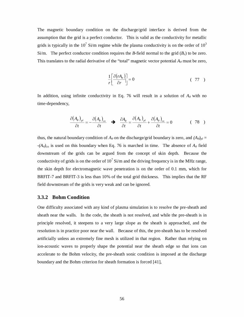
56
The magnetic boundary condition on the discharge/grid interface is derived from the
assumption that the grid is a perfect conductor. This is valid as the conductivity for metallic
grids is typically in the 107 Si/m regime while the plasma conductivity is on the order of 103
Si/m. The perfect conductor condition requires the B-field normal to the grid (Bz) to be zero.
This translates to the radial derivative of the “total” magnetic vector potential Aθ must be zero,
01
r
rAr
( 77 )
In addition, using infinite conductivity in Eq. 76 will result in a solution of Aθ with no
time-dependency,
t
At
Acopl
0
tA
tA
tA copl ( 78 )
thus, the natural boundary condition of Aθ on the discharge/grid boundary is zero, and (Aθ)pl =
-(Aθ)co is used on this boundary when Eq. 76 is marched in time. The absence of Aθ field
downstream of the grids can be argued from the concept of skin depth. Because the
conductivity of grids is on the order of 107 Si/m and the driving frequency is in the MHz range,
the skin depth for electromagnetic wave penetration is on the order of 0.1 mm, which for
BRFIT-7 and BRFIT-3 is less than 10% of the total grid thickness. This implies that the RF
field downstream of the grids is very weak and can be ignored.
3.3.2 Bohm Condition
One difficulty associated with any kind of plasma simulation is to resolve the pre-sheath and
sheath near the walls. In the code, the sheath is not resolved, and while the pre-sheath is in
principle resolved, it steepens to a very large slope as the sheath is approached, and the
resolution is in practice poor near the wall. Because of this, the pre-sheath has to be resolved
artificially unless an extremely fine mesh is utilized in that region. Rather than relying on
ion-acoustic waves to properly shape the potential near the sheath edge so that ions can
accelerate to the Bohm velocity, the pre-sheath sonic condition is imposed at the discharge
boundary and the Bohm criterion for sheath formation is forced [41],

57
i
eBohmboundaryi m
kTuu , ( 79 )
There are two ways the plasma density at the boundary can be updated. One is to rely on the
time-advancing feature of the ion conservation equation (Eq. 54) without the ionization term.
The other is to force flux conservation normal to the boundary as described by Ref. 41,
Bohm
normalboundarye u
n , ( 80 )
Both methods are adequate. However, utilizing Eq. 54 to update the boundary density takes
slightly longer time to converge. On the other hand, forcing the normal flux conservation is a
faster method but can cause numerical instability at low gas pressures as it would tend to “pull”
the plasma toward the wall at a faster rate. The code employs Eq. 80 as default for updating
plasma density at the boundary. This is to take advantage of its speedier convergence.
Based on the sonic condition at the presheath edge, zero electric potential is set at the numerical
discharge boundary that represents the sheath edge [23]. This corresponds to the wall being
charged negatively with respect to the plasma, which is a physical phenomenon.
3.3.3 Numerical Solution
A five-point finite-differencing scheme (Figure 24) is used throughout the discharge model for
discretizing the differential fluid equations. This approach is simple and typical of CFD
simulation on a structured orthogonal mesh. The code was not optimized for computing speed
as this was not within the scope of this research. Elliptic differential equations after
discretization are solved by MATLAB’s direct solver via Gaussian Elimination. Due to the
relative coarseness of the mesh, the direct solver actually performs pretty fast and no iterative
solution method is required. A successive over-relaxation iterative method will need to be
used if the mesh is further refined. The discretized equations shown in this section use
subscript [S,W,C,E,N] to represent positions in space and superscript [t, t-1] for positions in
time.

58
Figure 24 Five-Point Finite-Differencing Scheme
Solution to the magnetic field coupling and diffusion in the ICP discharge is found by
expanding and discretizing Eq. 76,
t
Ar
A
dr
A
rdz
A
dr
A
t
Acoplplplplpl
22
2
2
2
0
11 ( 81 )
The discretization begins in the time-domain with the use of time-step t ,
12
11
2
12
2
12
0
1 1
tco
tco
t
pl
t
pl
t
pl
t
plt
t
pl
t
pl
AA
rA
drA
rdzA
drAtAA
( 82 )
and is followed by spatial-discretization,
59
1
1
2
11
2
111
2
111
0
1
12
12
2
t
Ccot
Cco
t
CplC
t
Spl
t
Npl
C
t
Wpl
t
Cpl
t
Epl
t
Spl
t
Cpl
t
Nplt
C
t
Cpl
t
Cpl
AA
Arr
AA
rz
AAA
r
AAAtAA
( 83 )
Rearrange to Eq. 83 and collect like-terms in space to get
t
Cpl
t
Npl
t
Epl
t
Cpl
t
Wpl
t
Spl ACACACACACAC
6
1
5
1
4
1
3
1
2
1
1
with
Ct
Crrr
tC2
112
01
20
21z
tC t
C
2220
31221C
t
Crzr
tC
20
41z
tC t
C
Ct
Crrr
tC2
112
05
16
t
Ccot
Cco AAC
( 84 )
In matrix operations with a NN mesh set up in the discharge zone, Eq. 84 is represented as
60
6
1 CAQA tt
( 85 )
where Q is a 22 NN sparse matrix containing the coefficients 1C to 5C , and tA
, 1tA
and
6C
are 12 N column vectors. The 6C
vector represents the coil-induced background field
discussed previously.
The solution scheme for plA in free space is a little different as it cannot be advanced in
time. Based on Eq. 75, the discretization becomes
01
21
22
2
22
CplC
SplNpl
C
WplCplEplSplCplNpl
Arr
AA
r
z
AAA
r
AAA
( 86 )
which can be reduced to matrix operation fAQ
with f
being a null vector and Q being
the sparse matrix containing the coefficients C1 to C5,
Crrr
C
2
1121
221z
C
2223122
CrzrC
241z
C
CrrrC
211
25
61
Numerical solution scheme to the electric potential equation (Eq. 59) is similar to the above.
Discretization on the left-hand-side involves treating the conductivity as a local parameter,
22
22
2222
zr
zzrrr
LHS
WCEC
SCNC
WEWESN
C
CSN
( 87 )
and the matrix coefficients become
NECWS CCCCCLHS 54321
21 221
rrrrC C
C
CSN
22 221
zzzC CWE
22322
zrC CC
24 221
zzzC CWE
25 221
rrrrC C
C
CSN
The right-hand-side of Eq. 59 is discretized in a similar fashion and the resultant values serve
as the forcing term in the matrix equation.

62
3.4 Ion Optics
The ICP discharge code does not have a built-in ion optics simulation. Rather, a grid ion
transparency function published in the literature is implemented for the purpose of verifying
the code with experimental data. Because both the BRFIT-7 and the BRFIT-3 thrusters utilize
a similar grid design as the NEXT ion engine developed by NASA, simulation results for the
NEXT ion optics can be adopted. Farnell [30] has published such a simulation with Colorado
State University’s three-dimensional charge-exchange ion optics code named ffx. Details of
the ffx code can be found in Ref. 30. One set of the simulation parameters closely resembles
the experimental condition of BRFIT-7 and BRFIT-3. These parameters are listed in Table 1.
The effective grid transparency to ions as calculated by the ffx code under these conditions is
shown in Figure 25. Figure 25 also contains the results of other ion optics code (igx, CEX2D,
and CEX3D), but they are not considered in this thesis because the ffx code has demonstrated
very good agreement with the experimental data of NASA’s NSTAR ion engine [30]. Since
the ion optics of the NEXT thruster is very similar to that of the NSTAR thruster, the ffx code is
considered reliable in this instance.
The discharge code incorporates a curve-fit function of the ffx simulation result. The anode
current (approximately equal to the ion beam current) is then found by multiplying the ion flux
reaching the grid with the grid ion transparency and integrating over the grid area,
grid
ionBohmboundaryeanode dAuneJ , ( 88 )
where ne,boundary is the plasma density at the discharge boundary in front of the grid, uBohm is the
sonic velocity of ions, and ion is the ion transparency function found in Figure 25.
Table 1 Parameters for Grid Ion Transparency Simulation [30]
Screen Grid Voltage 1800 V
Accelerator Grid Voltage -210 V
Beam Plasma Potential 10 V
Source Electron Temperature 6 eV
Grid Spacing-to-Screen Aperture Diameter Ratio 0.347
Physical Open Fraction of Screen Grid 67%

63
Figure 25 Ion Transparency Simulation Published by Farnell [30]
64
Chapter 4
RESULTS
Results of the ICP discharge code are presented in this chapter. The transformer sub-model is
first shown being able to predict the operating frequency and the circuit capacitance required to
maximize RF power coupling efficiency. This part of the design work can be done without
executing the main discharge simulation, but does require a guess on the averaged plasma
conductivity. Since plasma conductivity is a function of operating condition, the discharge
simulation becomes useful in verifying the optimum driving frequency.
BRFIT-7 experiment data were used to compare with the simulation results. This benchmark
verification is detailed in Section 4.2. Scaling-capability of the code was demonstrated by
data comparison with the smaller BRFIT-3 thruster. This result is presented in Section 4.3.
Section 4.4 is an optimization study that aims to improve the performance of BRFIT-3 with the
use of the discharge simulation. In this chapter, proprietary data of BRFIT-7 and BRFIT-3 are
intentionally obscured; these include their operating frequencies and circuit capacitance values.
The discharge geometries depicted by the simulation results also do not represent the exact
physical dimensions of these two thrusters.
A flowchart of the code can be found in Figure 26. It illustrates how the computation
progresses at each time-step, although some parameters do not need to be solved in the
specified order. Computation of the baseline background coil-induced magnetic field must be
carried out every time when there is a change in wave resolution (number of points discretizing
the wave period) or a change in geometry (i.e. coil location, number of turns, size of the
discharge chamber, etc.). This baseline background field is generated with 1A RMS
sinusoidal coil current and is independent of operating frequency. Frequency is resolved from
the definition of time-step (Eq. 8). The real-time coil-induced magnetic field is found within
each time-step by accessing the pre-computed baseline data and augmenting it with the coil
current obtained from the transformer model.

65
Figure 26 Flowchart of the ICP Discharge Code
4.1 Matching Circuit Design
A variation of the transformer model employed by the ICP discharge code can be executed
independently to aid the matching circuit design. The transfer model by itself does not require
RF power as input because its main function is to compute impedance of circuit elements.
The impedance due to plasma loading can be simulated by prescribing an averaged plasma
conductivity. As long as proper coil and chamber geometries are defined, the transformer
model can optimize the power coupling efficiency of the matching circuit by sweeping through
frequency and parallel capacitance value. Again, the power coupling efficiency is defined as
(1 – power reflection %). Figure 27 shows the circuit design for the BRFIT-7 thruster,
Compute r-z plane electric potential
Update r-z plane ion velocity
Compute plasma conductivity
Obtain ionization and excitation rates
Update magnetic vector potential field
Compute induced plasma current
Update electron density
Update electron temperature
Compute anode current
Update neutral density
Compute coil current (transformer model)
Update background coil-induced magnetic field
Load baseline background coil-induced magnetic field
Initialize variables
Load energy-averaged cross section data
Δt

66
assuming a plasma conductivity of 500 Si/m. The minimum power reflection, or the
maximum power coupling efficiency, occurs between 1.2 and 1.3 MHz frequency with
corresponding parallel capacitance between 32,000 and 38,000 pico-farad. These values
closely resemble to the BRFIT-7 circuit, design which was empirically optimized. The catch
of this circuit design method is that plasma conductivity must be estimated correctly. For
example, Figure 28 shows the same design approach, but using a higher conductivity of 1000
Si/m. The optimum frequency is pushed up to the 1.9-2.1 MHz range and the optimum
capacitance drops below 27,000 pf. Experimentally BRFIT-7 cannot operate in this regime
efficiently, so the 1000 Si/m is definitely an over-estimate. This analysis shows that while the
transformer model by itself can approximate the desirable operating frequency and its
corresponding circuit capacitance, true optimization must be performed by the discharge
simulation as the true plasma conductivity is not known a priori. In practice the capacitance
and the frequency are designed for a nominal operating condition that matches to a certain
plasma conductivity. As discharge conditions change, one can either vary the frequency or
accept the penalty in coupling efficiency. Varying capacitance is also feasible, but the
bulkiness of a variable capacitor is not practical for flight systems.
Figure 27 Matching Circuit Design for BRFIT-7 with the Transformer Model;
Plasma Conductivity is Assumed 500 Si/m

67
Figure 28 Matching Circuit Design for BRFIT-7 with the Transformer Model;
Plasma Conductivity is Assumed 1000 Si/m
4.2 Performance of ICP Discharge Code The performance of the discharge code is characterized by three categories: convergence,
validity, and scaling ability. The code convergence is described in Section 4.2.1. Section
4.2.2 validates the code with the experimental data of BRFIT-7. Lastly, Section 4.2.3 verifies
the scaling capability of the code by data comparison with BRFIT-3.
4.2.1 Convergence
The convergence of a time-dependent RF plasma simulation is difficult to define due to the
nature of high-frequency oscillation. For the ICP discharge code, convergence is defined by
observing steady-state (or cyclic steady-state) outputs for all the following quantities: 1)
electron temperature, 2) plasma dissipation power calculated from dVj 2 , 3) plasma
internal power losses due to ionization, excitation and ion wall loss, 4) circuit ohmic heating
loss calculated from RMS coil current and circuit resistance, and 5) anode current. The
dissipated power ideally must equal the sum of the three internal power losses. And the sum
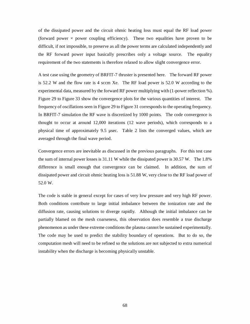
68
of the dissipated power and the circuit ohmic heating loss must equal the RF load power
(forward power × power coupling efficiency). These two equalities have proven to be
difficult, if not impossible, to preserve as all the power terms are calculated independently and
the RF forward power input basically prescribes only a voltage source. The equality
requirement of the two statements is therefore relaxed to allow slight convergence error.
A test case using the geometry of BRFIT-7 thruster is presented here. The forward RF power
is 52.2 W and the flow rate is 4 sccm Xe. The RF load power is 52.0 W according to the
experimental data, measured by the forward RF power multiplying with (1-power reflection %).
Figure 29 to Figure 33 show the convergence plots for the various quantities of interest. The
frequency of oscillations seen in Figure 29 to Figure 31 corresponds to the operating frequency.
In BRFIT-7 simulation the RF wave is discretized by 1000 points. The code convergence is
thought to occur at around 12,000 iterations (12 wave periods), which corresponds to a
physical time of approximately 9.5 µsec. Table 2 lists the converged values, which are
averaged through the final wave period.
Convergence errors are inevitable as discussed in the previous paragraphs. For this test case
the sum of internal power losses is 31.11 W while the dissipated power is 30.57 W. The 1.8%
difference is small enough that convergence can be claimed. In addition, the sum of
dissipated power and circuit ohmic heating loss is 51.88 W, very close to the RF load power of
52.0 W.
The code is stable in general except for cases of very low pressure and very high RF power.
Both conditions contribute to large initial imbalance between the ionization rate and the
diffusion rate, causing solutions to diverge rapidly. Although the initial imbalance can be
partially blamed on the mesh coarseness, this observation does resemble a true discharge
phenomenon as under these extreme conditions the plasma cannot be sustained experimentally.
The code may be used to predict the stability boundary of operations. But to do so, the
computation mesh will need to be refined so the solutions are not subjected to extra numerical
instability when the discharge is becoming physically unstable.

69
Table 2 Converged Values from Discharge Simulation
Parameter Definition Value
Te electron temperature 3.2 eV
Dissipated Power dVj 2 30.57 W
Ionization Power dVeVn ie 6.31 W
Excitation Power dVeVn excexc 9.91 W
Wall Loss Power dAekT wallsheathe 2 14.89 W
Circuit Ohmic Heating Loss circuitcoilRMS RJ 2, 21.31 W
Anode Current grid
ionBohmboundarye dAune ,
143.7 mA
Figure 29 Convergence of Electron Temperature in the BRFIT-7 Simulation; Each
Iteration Represents 7.7×10⁻¹⁰ Seconds in Real Time
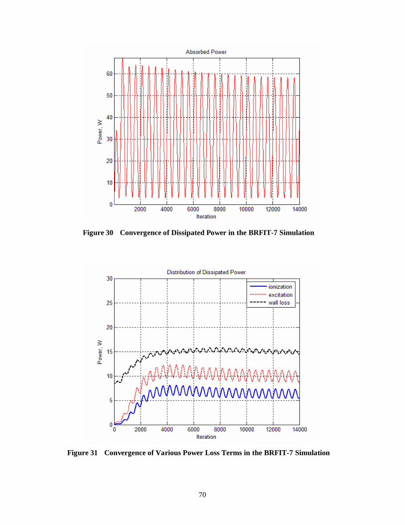
70
Figure 30 Convergence of Dissipated Power in the BRFIT-7 Simulation
Figure 31 Convergence of Various Power Loss Terms in the BRFIT-7 Simulation
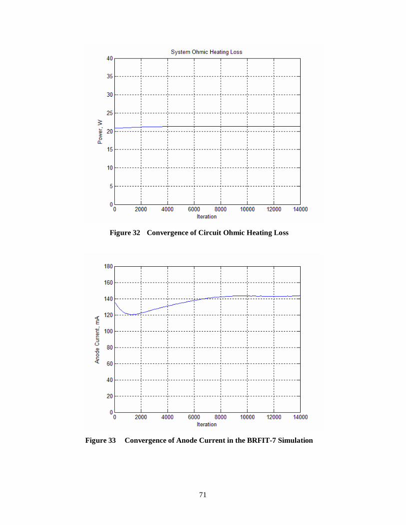
71
Figure 32 Convergence of Circuit Ohmic Heating Loss
Figure 33 Convergence of Anode Current in the BRFIT-7 Simulation
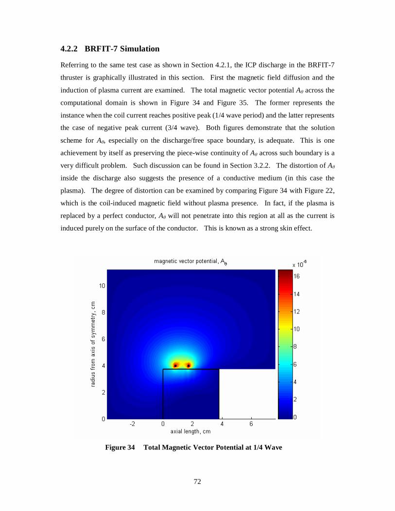
72
4.2.2 BRFIT-7 Simulation
Referring to the same test case as shown in Section 4.2.1, the ICP discharge in the BRFIT-7
thruster is graphically illustrated in this section. First the magnetic field diffusion and the
induction of plasma current are examined. The total magnetic vector potential Aθ across the
computational domain is shown in Figure 34 and Figure 35. The former represents the
instance when the coil current reaches positive peak (1/4 wave period) and the latter represents
the case of negative peak current (3/4 wave). Both figures demonstrate that the solution
scheme for Aθ, especially on the discharge/free space boundary, is adequate. This is one
achievement by itself as preserving the piece-wise continuity of Aθ across such boundary is a
very difficult problem. Such discussion can be found in Section 3.2.2. The distortion of Aθ
inside the discharge also suggests the presence of a conductive medium (in this case the
plasma). The degree of distortion can be examined by comparing Figure 34 with Figure 22,
which is the coil-induced magnetic field without plasma presence. In fact, if the plasma is
replaced by a perfect conductor, Aθ will not penetrate into this region at all as the current is
induced purely on the surface of the conductor. This is known as a strong skin effect.
Figure 34 Total Magnetic Vector Potential at 1/4 Wave
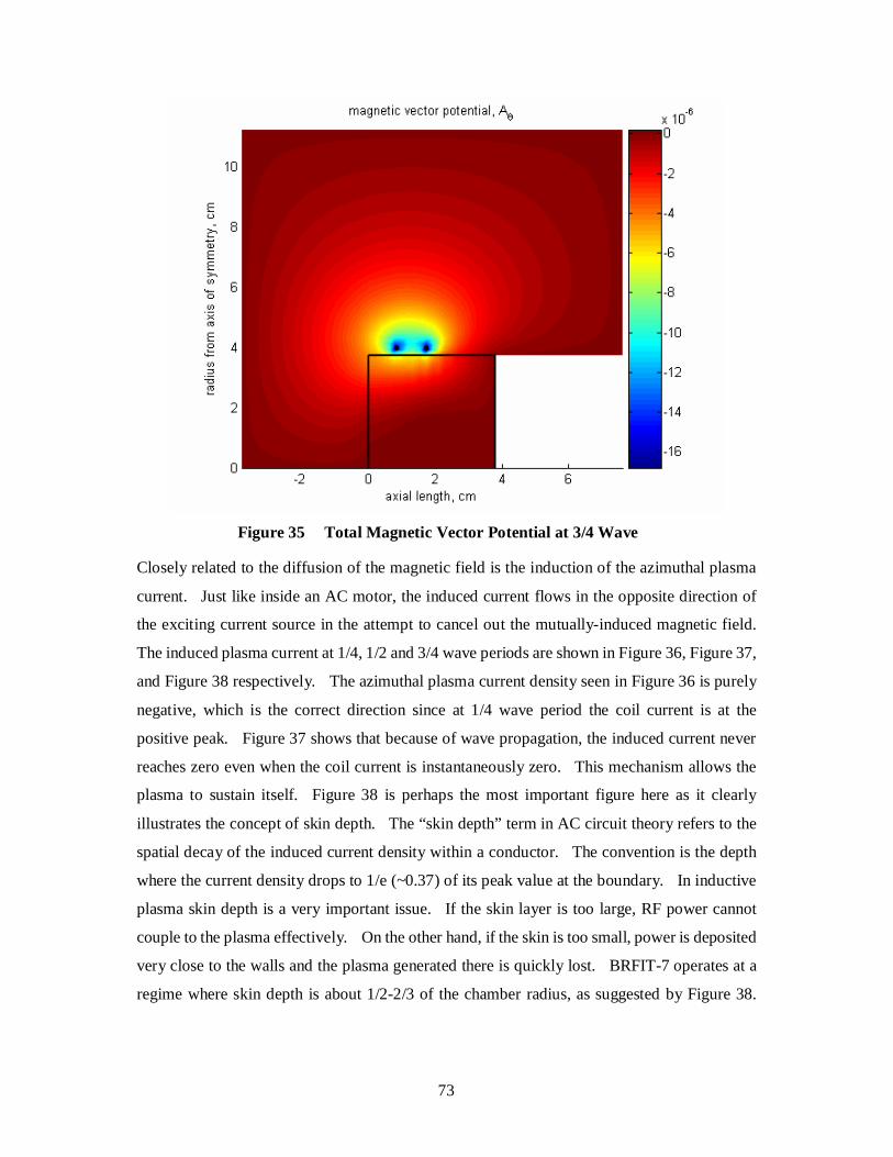
73
Figure 35 Total Magnetic Vector Potential at 3/4 Wave
Closely related to the diffusion of the magnetic field is the induction of the azimuthal plasma
current. Just like inside an AC motor, the induced current flows in the opposite direction of
the exciting current source in the attempt to cancel out the mutually-induced magnetic field.
The induced plasma current at 1/4, 1/2 and 3/4 wave periods are shown in Figure 36, Figure 37,
and Figure 38 respectively. The azimuthal plasma current density seen in Figure 36 is purely
negative, which is the correct direction since at 1/4 wave period the coil current is at the
positive peak. Figure 37 shows that because of wave propagation, the induced current never
reaches zero even when the coil current is instantaneously zero. This mechanism allows the
plasma to sustain itself. Figure 38 is perhaps the most important figure here as it clearly
illustrates the concept of skin depth. The “skin depth” term in AC circuit theory refers to the
spatial decay of the induced current density within a conductor. The convention is the depth
where the current density drops to 1/e (~0.37) of its peak value at the boundary. In inductive
plasma skin depth is a very important issue. If the skin layer is too large, RF power cannot
couple to the plasma effectively. On the other hand, if the skin is too small, power is deposited
very close to the walls and the plasma generated there is quickly lost. BRFIT-7 operates at a
regime where skin depth is about 1/2-2/3 of the chamber radius, as suggested by Figure 38.
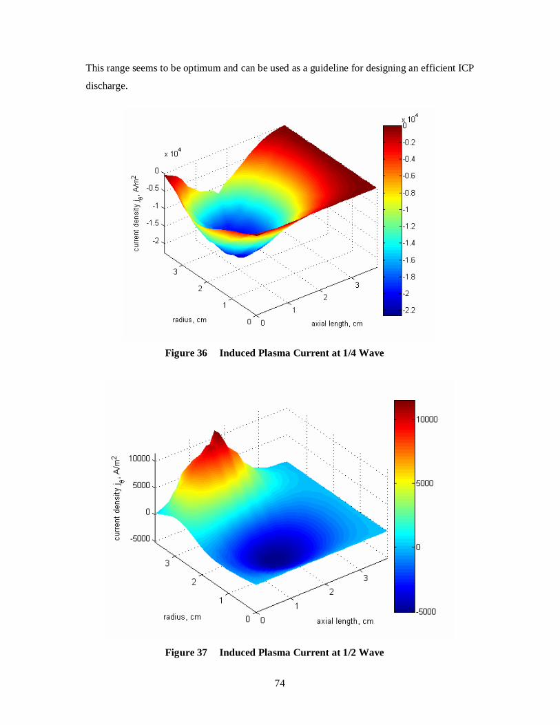
74
This range seems to be optimum and can be used as a guideline for designing an efficient ICP
discharge.
Figure 36 Induced Plasma Current at 1/4 Wave
Figure 37 Induced Plasma Current at 1/2 Wave

75
Figure 38 Induced Plasma Current at 3/4 Wave
The skin depth can also be observed through the distribution of the dissipated power, which is
found by the ohmic heating of the induced current density within a discretized volume,
dVj 2 . This is illustrated in Figure 39 to Figure 41. Through this mechanism the
plasma receives the energy for supporting ionization. The spatial decay of the power
dissipation is an extension to the skin depth description. From Figure 39 and Figure 41, a skin
depth of 1/2 chamber radius can be concluded. It is also noted that maximum power
deposition occurs every half wave period (1/4 and 3/4 wave).
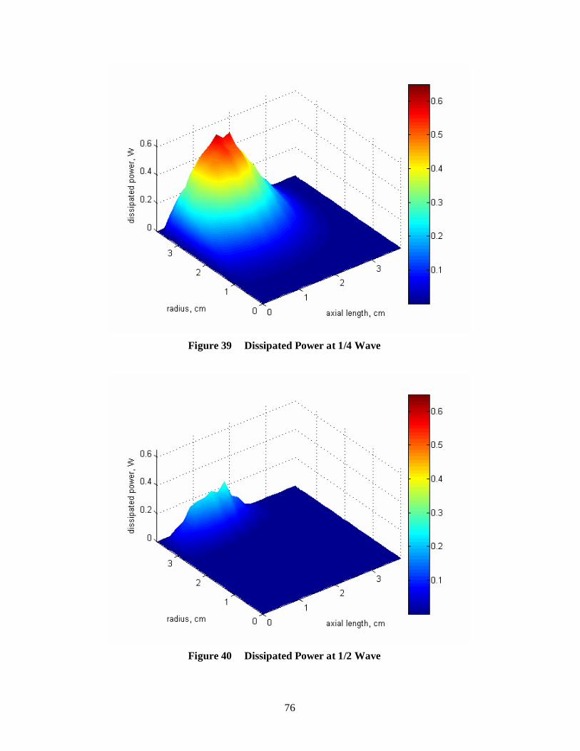
76
Figure 39 Dissipated Power at 1/4 Wave
Figure 40 Dissipated Power at 1/2 Wave
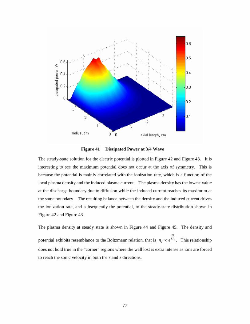
77
Figure 41 Dissipated Power at 3/4 Wave
The steady-state solution for the electric potential is plotted in Figure 42 and Figure 43. It is
interesting to see the maximum potential does not occur at the axis of symmetry. This is
because the potential is mainly correlated with the ionization rate, which is a function of the
local plasma density and the induced plasma current. The plasma density has the lowest value
at the discharge boundary due to diffusion while the induced current reaches its maximum at
the same boundary. The resulting balance between the density and the induced current drives
the ionization rate, and subsequently the potential, to the steady-state distribution shown in
Figure 42 and Figure 43.
The plasma density at steady state is shown in Figure 44 and Figure 45. The density and
potential exhibits resemblance to the Boltzmann relation, that is ekTe
e en
. This relationship
does not hold true in the “corner” regions where the wall lost is extra intense as ions are forced
to reach the sonic velocity in both the r and z directions.

78
Figure 42 Electric Potential Distribution
Figure 43 Electric Potential Distribution (Planar View)

79
Figure 44 Plasma Density Distribution
Figure 45 Plasma Density Distribution (Planar View)
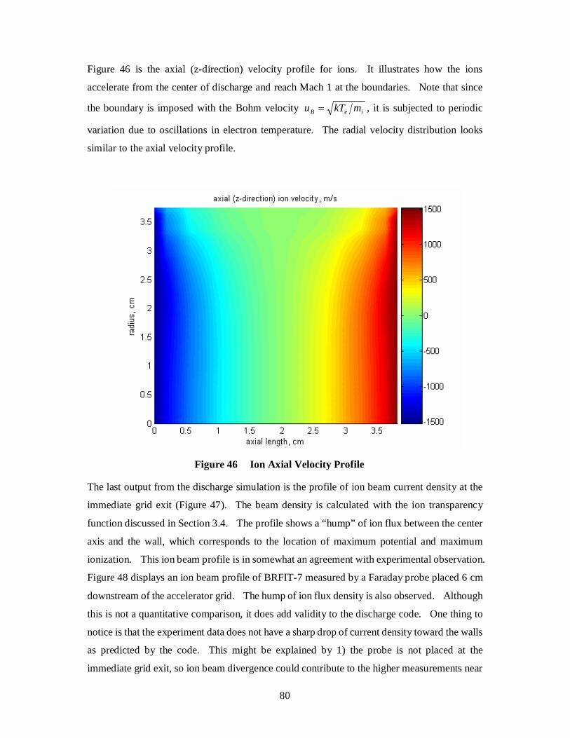
80
Figure 46 is the axial (z-direction) velocity profile for ions. It illustrates how the ions
accelerate from the center of discharge and reach Mach 1 at the boundaries. Note that since
the boundary is imposed with the Bohm velocity ieB mkTu , it is subjected to periodic
variation due to oscillations in electron temperature. The radial velocity distribution looks
similar to the axial velocity profile.
Figure 46 Ion Axial Velocity Profile
The last output from the discharge simulation is the profile of ion beam current density at the
immediate grid exit (Figure 47). The beam density is calculated with the ion transparency
function discussed in Section 3.4. The profile shows a “hump” of ion flux between the center
axis and the wall, which corresponds to the location of maximum potential and maximum
ionization. This ion beam profile is in somewhat an agreement with experimental observation.
Figure 48 displays an ion beam profile of BRFIT-7 measured by a Faraday probe placed 6 cm
downstream of the accelerator grid. The hump of ion flux density is also observed. Although
this is not a quantitative comparison, it does add validity to the discharge code. One thing to
notice is that the experiment data does not have a sharp drop of current density toward the walls
as predicted by the code. This might be explained by 1) the probe is not placed at the
immediate grid exit, so ion beam divergence could contribute to the higher measurements near

81
the walls, and 2) the collector area of the Faraday probe is finite, which could average out the
ion flux over a relatively large area.
Figure 47 Simulated Ion Beam Current Density Profile
0
5
10
15
20
25
30
35
0 1 2 3 4
Radial location from centerline, cm
Fara
day
prob
e da
ta
Figure 48 Ion Beam Flux Profile Measured by a Faraday Probe
Three additional experimental data points from BRFIT-7 were used for comparison. The
results are presented in Table 3. The anode current data are plotted in Figure 49. Two
observations can be made. First, the load power (plasma dissipated power + circuit ohmic
heating loss) is correctly simulated. This has been a difficult task as there are many
parameters involved in finding the load power. Getting a correct match on the power means
all the sub-models regarding ionization, excitation, wall loss, and current induction are valid to

82
some extent. Relative errors however might exist, but there are no data on the internal losses
that can be compared with. Second, the anode current prediction is pretty accurate (2% error
or less) at high RF power, but falters at low power (20% error). The source of this discrepancy
has not been found as for the BRFIT-3 case shown in the next section the opposite is true. The
employed ion transparency function was deemed a non-factor in this issue.
Table 3 Results Comparison for BRFIT-7 Simulation
Experiment Simulation
Flow, sccm Pforward, W Pload, W Janode, mA Pload, W Janode, mA 4 42.4 42.2 109.4 42.6 131.0 4 52.2 52.0 133.0 51.9 143.7 4 62.6 62.4 155.8 61.6 156.9 4 67.8 67.6 166.4 66.3 163.3
60
80
100
120
140
160
180
200
30 40 50 60 70 80
Forward RF Power, W
Anod
e Cu
rren
t, m
A
Anode Current, Exp Anode Current, Sim
Figure 49 Anode Current Comparison for BRFIT-7
4.2.3 BRFIT-3 Simulation
Based on good agreements with the experimental data from BRFIT-7, the discharge code is
applied to BRFIT-3 to verify its scaling capability. The code is not altered in any way except
for geometrical changes. The Knudsen number is first examined to ensure the fluid
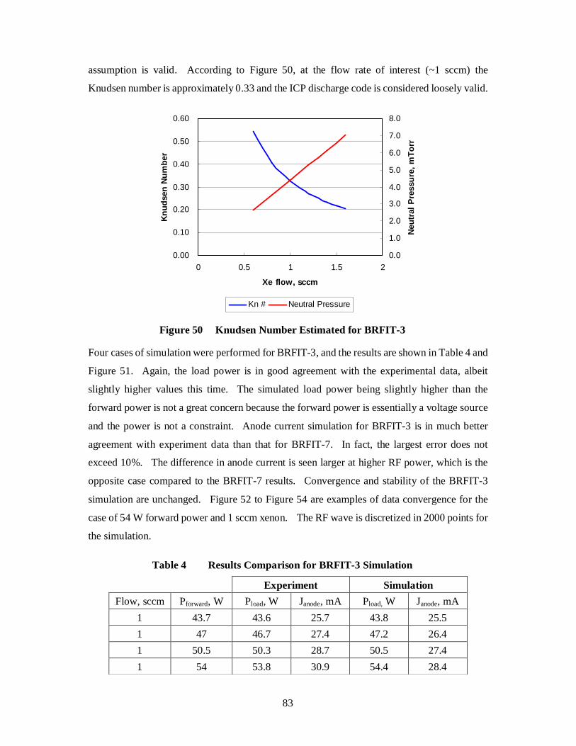
83
assumption is valid. According to Figure 50, at the flow rate of interest (~1 sccm) the
Knudsen number is approximately 0.33 and the ICP discharge code is considered loosely valid.
0.00
0.10
0.20
0.30
0.40
0.50
0.60
0 0.5 1 1.5 2
Xe flow, sccm
Knud
sen
Num
ber
0.0
1.0
2.0
3.0
4.0
5.0
6.0
7.0
8.0
Neut
ral P
ress
ure,
mTo
rr
Kn # Neutral Pressure
Figure 50 Knudsen Number Estimated for BRFIT-3
Four cases of simulation were performed for BRFIT-3, and the results are shown in Table 4 and
Figure 51. Again, the load power is in good agreement with the experimental data, albeit
slightly higher values this time. The simulated load power being slightly higher than the
forward power is not a great concern because the forward power is essentially a voltage source
and the power is not a constraint. Anode current simulation for BRFIT-3 is in much better
agreement with experiment data than that for BRFIT-7. In fact, the largest error does not
exceed 10%. The difference in anode current is seen larger at higher RF power, which is the
opposite case compared to the BRFIT-7 results. Convergence and stability of the BRFIT-3
simulation are unchanged. Figure 52 to Figure 54 are examples of data convergence for the
case of 54 W forward power and 1 sccm xenon. The RF wave is discretized in 2000 points for
the simulation.
Table 4 Results Comparison for BRFIT-3 Simulation
Experiment Simulation Flow, sccm Pforward, W Pload, W Janode, mA Pload, W Janode, mA
1 43.7 43.6 25.7 43.8 25.5 1 47 46.7 27.4 47.2 26.4 1 50.5 50.3 28.7 50.5 27.4 1 54 53.8 30.9 54.4 28.4
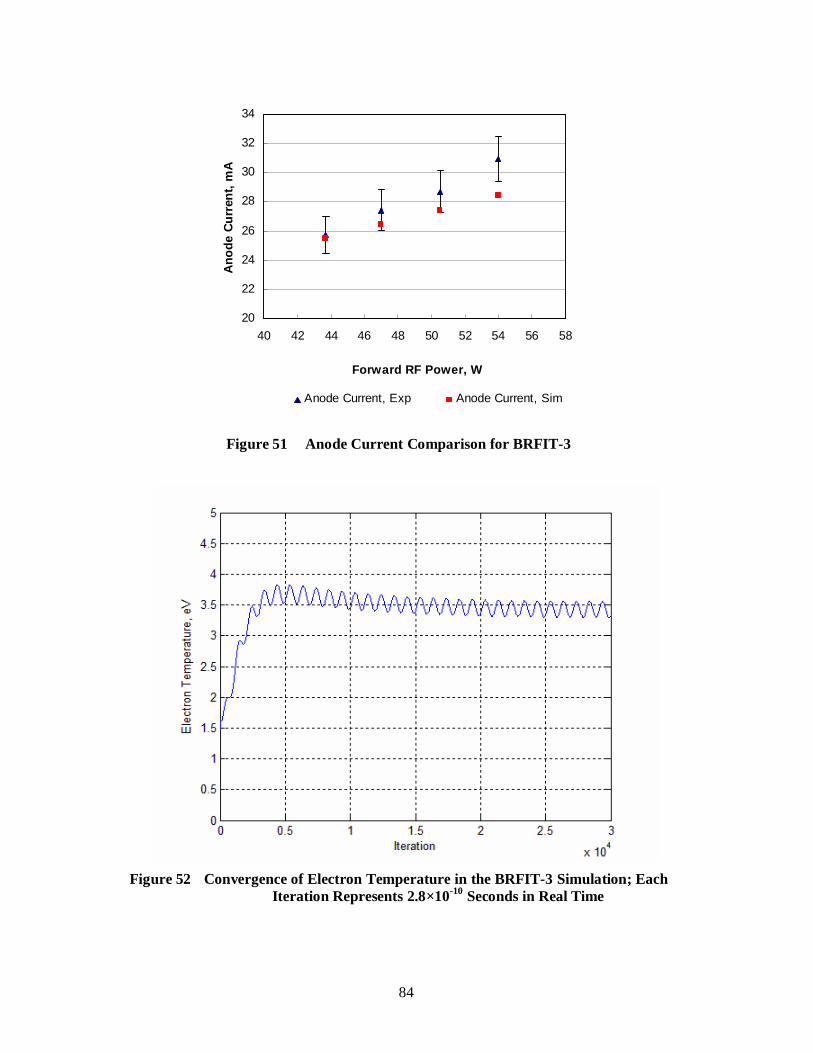
84
20
22
24
26
28
30
32
34
40 42 44 46 48 50 52 54 56 58
Forward RF Power, W
Ano
de C
urre
nt, m
A
Anode Current, Exp Anode Current, Sim
Figure 51 Anode Current Comparison for BRFIT-3
Figure 52 Convergence of Electron Temperature in the BRFIT-3 Simulation; Each
Iteration Represents 2.8×10⁻¹⁰ Seconds in Real Time
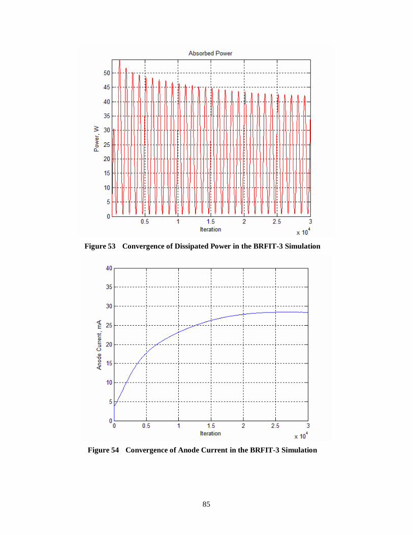
85
Figure 53 Convergence of Dissipated Power in the BRFIT-3 Simulation
Figure 54 Convergence of Anode Current in the BRFIT-3 Simulation
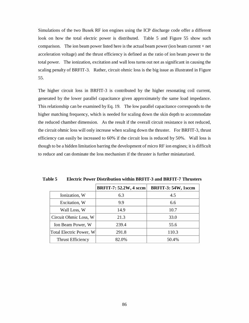
86
Simulations of the two Busek RF ion engines using the ICP discharge code offer a different
look on how the total electric power is distributed. Table 5 and Figure 55 show such
comparison. The ion beam power listed here is the actual beam power (ion beam current × net
acceleration voltage) and the thrust efficiency is defined as the ratio of ion beam power to the
total power. The ionization, excitation and wall loss turns out not as significant in causing the
scaling penalty of BRFIT-3. Rather, circuit ohmic loss is the big issue as illustrated in Figure
55.
The higher circuit loss in BRFIT-3 is contributed by the higher resonating coil current,
generated by the lower parallel capacitance given approximately the same load impedance.
This relationship can be examined by Eq. 19. The low parallel capacitance corresponds to the
higher matching frequency, which is needed for scaling down the skin depth to accommodate
the reduced chamber dimension. As the result if the overall circuit resistance is not reduced,
the circuit ohmic loss will only increase when scaling down the thruster. For BRFIT-3, thrust
efficiency can easily be increased to 60% if the circuit loss is reduced by 50%. Wall loss is
though to be a hidden limitation barring the development of micro RF ion engines; it is difficult
to reduce and can dominate the loss mechanism if the thruster is further miniaturized.
Table 5 Electric Power Distribution within BRFIT-3 and BRFIT-7 Thrusters
BRFIT-7: 52.2W, 4 sccm BRFIT-3: 54W, 1sccm Ionization, W 6.3 4.5 Excitation, W 9.9 6.6 Wall Loss, W 14.9 10.7
Circuit Ohmic Loss, W 21.3 33.0 Ion Beam Power, W 239.4 55.6
Total Electric Power, W 291.8 110.3 Thrust Efficiency 82.0% 50.4%
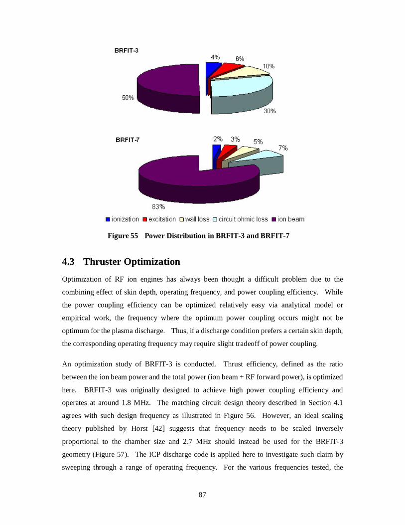
87
Figure 55 Power Distribution in BRFIT-3 and BRFIT-7
4.3 Thruster Optimization
Optimization of RF ion engines has always been thought a difficult problem due to the
combining effect of skin depth, operating frequency, and power coupling efficiency. While
the power coupling efficiency can be optimized relatively easy via analytical model or
empirical work, the frequency where the optimum power coupling occurs might not be
optimum for the plasma discharge. Thus, if a discharge condition prefers a certain skin depth,
the corresponding operating frequency may require slight tradeoff of power coupling.
An optimization study of BRFIT-3 is conducted. Thrust efficiency, defined as the ratio
between the ion beam power and the total power (ion beam + RF forward power), is optimized
here. BRFIT-3 was originally designed to achieve high power coupling efficiency and
operates at around 1.8 MHz. The matching circuit design theory described in Section 4.1
agrees with such design frequency as illustrated in Figure 56. However, an ideal scaling
theory published by Horst [42] suggests that frequency needs to be scaled inversely
proportional to the chamber size and 2.7 MHz should instead be used for the BRFIT-3
geometry (Figure 57). The ICP discharge code is applied here to investigate such claim by
sweeping through a range of operating frequency. For the various frequencies tested, the
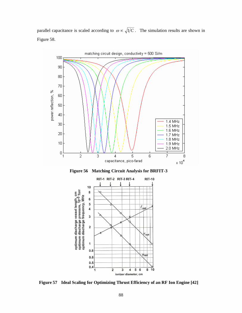
88
parallel capacitance is scaled according to C1 . The simulation results are shown in
Figure 58.
Figure 56 Matching Circuit Analysis for BRFIT-3
Figure 57 Ideal Scaling for Optimizing Thrust Efficiency of an RF Ion Engine [42]
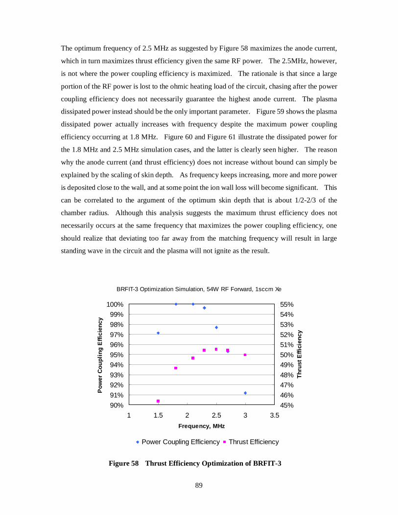
89
The optimum frequency of 2.5 MHz as suggested by Figure 58 maximizes the anode current,
which in turn maximizes thrust efficiency given the same RF power. The 2.5MHz, however,
is not where the power coupling efficiency is maximized. The rationale is that since a large
portion of the RF power is lost to the ohmic heating load of the circuit, chasing after the power
coupling efficiency does not necessarily guarantee the highest anode current. The plasma
dissipated power instead should be the only important parameter. Figure 59 shows the plasma
dissipated power actually increases with frequency despite the maximum power coupling
efficiency occurring at 1.8 MHz. Figure 60 and Figure 61 illustrate the dissipated power for
the 1.8 MHz and 2.5 MHz simulation cases, and the latter is clearly seen higher. The reason
why the anode current (and thrust efficiency) does not increase without bound can simply be
explained by the scaling of skin depth. As frequency keeps increasing, more and more power
is deposited close to the wall, and at some point the ion wall loss will become significant. This
can be correlated to the argument of the optimum skin depth that is about 1/2-2/3 of the
chamber radius. Although this analysis suggests the maximum thrust efficiency does not
necessarily occurs at the same frequency that maximizes the power coupling efficiency, one
should realize that deviating too far away from the matching frequency will result in large
standing wave in the circuit and the plasma will not ignite as the result.
BRFIT-3 Optimization Simulation, 54W RF Forward, 1sccm Xe
90%91%92%93%94%95%96%97%98%99%
100%
1 1.5 2 2.5 3 3.5Frequency, MHz
Pow
er C
oupl
ing
Effi
cien
cy
45%46%47%48%49%50%51%52%53%54%55%
Thru
st E
ffici
ency
Power Coupling Efficiency Thrust Efficiency
Figure 58 Thrust Efficiency Optimization of BRFIT-3
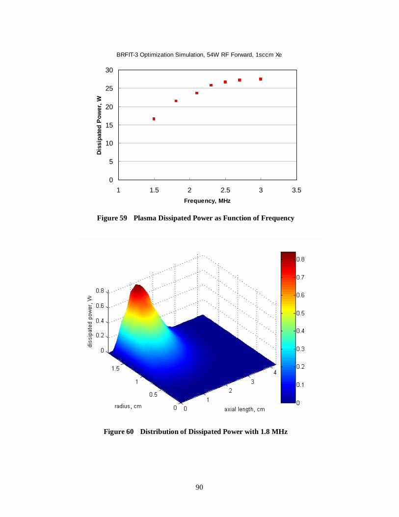
90
BRFIT-3 Optimization Simulation, 54W RF Forward, 1sccm Xe
0
5
10
15
20
25
30
1 1.5 2 2.5 3 3.5Frequency, MHz
Diss
ipat
ed P
ower
, W
Figure 59 Plasma Dissipated Power as Function of Frequency
Figure 60 Distribution of Dissipated Power with 1.8 MHz
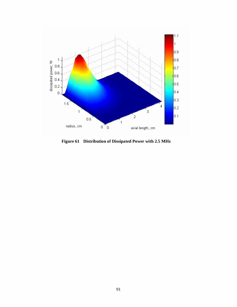
91
Figure 61 Distribution of Dissipated Power with 2.5 MHz
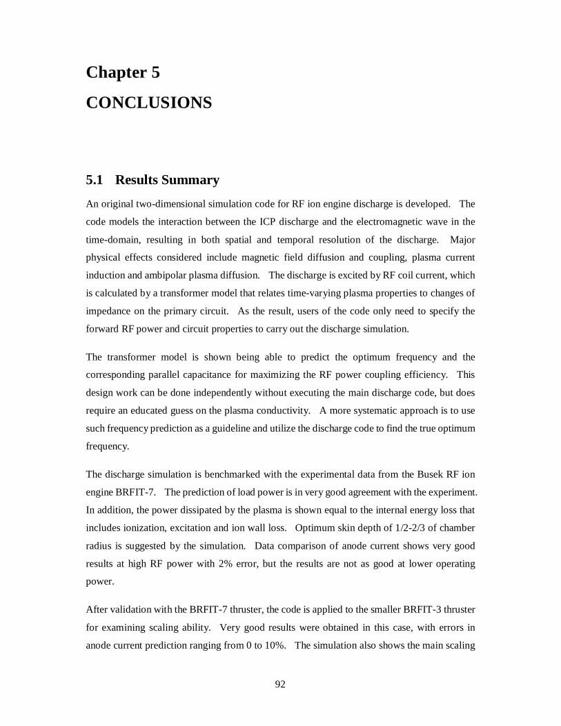
92
Chapter 5
CONCLUSIONS
5.1 Results Summary An original two-dimensional simulation code for RF ion engine discharge is developed. The
code models the interaction between the ICP discharge and the electromagnetic wave in the
time-domain, resulting in both spatial and temporal resolution of the discharge. Major
physical effects considered include magnetic field diffusion and coupling, plasma current
induction and ambipolar plasma diffusion. The discharge is excited by RF coil current, which
is calculated by a transformer model that relates time-varying plasma properties to changes of
impedance on the primary circuit. As the result, users of the code only need to specify the
forward RF power and circuit properties to carry out the discharge simulation.
The transformer model is shown being able to predict the optimum frequency and the
corresponding parallel capacitance for maximizing the RF power coupling efficiency. This
design work can be done independently without executing the main discharge code, but does
require an educated guess on the plasma conductivity. A more systematic approach is to use
such frequency prediction as a guideline and utilize the discharge code to find the true optimum
frequency.
The discharge simulation is benchmarked with the experimental data from the Busek RF ion
engine BRFIT-7. The prediction of load power is in very good agreement with the experiment.
In addition, the power dissipated by the plasma is shown equal to the internal energy loss that
includes ionization, excitation and ion wall loss. Optimum skin depth of 1/2-2/3 of chamber
radius is suggested by the simulation. Data comparison of anode current shows very good
results at high RF power with 2% error, but the results are not as good at lower operating
power.
After validation with the BRFIT-7 thruster, the code is applied to the smaller BRFIT-3 thruster
for examining scaling ability. Very good results were obtained in this case, with errors in
anode current prediction ranging from 0 to 10%. The simulation also shows the main scaling
93
penalty for BRFIT-3 is the circuit ohmic heating loss, which if reduced by 50% can help the
thruster achieve 60% thrust efficiency.
An optimization of thrust efficiency is conducted for BRFIT-3 with respect to the operating
frequency. The discharge code is employed to test the tradeoff between the power coupling
efficiency and the anode current. The results suggest the maximum thrust efficiency does not
necessarily occur at the same frequency that maximizes the power coupling efficiency, as the
ohmic heating loss in the circuit and the plasma skin depth both need to be considered. The
predicted optimum frequency is 2.5 MHz for maximizing the thrust efficiency, similar to the
value obtained from a published ideal scaling theory.
5.2 Contributions
The main contribution of this thesis work is the systematic approach to design an RF ion engine.
The simulation code serves a tool package that unifies the designs of matching circuit and ICP
discharge. The code is user-friendly in terms of user specified inputs and fast convergence.
The theory of magnetic field coupling and diffusion using a background coil-induced field as
the source term is also considered innovative. The two-dimensional solution of RF ion engine
discharge in time-domain is another innovation that was not found in literature research.
5.3 Recommendations for Future Work
Future work on this project includes the implementation of a self-consistent ion optics code.
The ion transparency function used in the model is very grid and voltage-specific and is not
intended for general purpose. Adaptation of a published ion optics code is possible, but most
likely it will be easier to write the code from scratch using the same MATLAB platform.
The solution for magnetic field should be extended to the plume region. Currently the plume
is assumed un-magnetized from the argument that the grids are conductive enough to shield the
electromagnetic wave penetration. The plume is also assumed non-divergent so the
cylindrical boundary between the plume and vacuum has zero magnetic field. Although these
assumptions are valid theoretically, extending the computation mesh to the plume region will
be a more rigorous approach. The grids will need to receive a fine mesh to resolve the RF
wave penetration.

94
The scheme that generates a piece-wise continuous solution of magnetic field across the
discharge/vacuum boundary should be revised. Though the current method works adequately,
it is perhaps best not to rely on the “slope correction factor” which requires some initial
trial-and-error every time when a new computation mesh is utilized. Other possible
slope-matching schemes should be pursued. One suggestion is to reduce the plasma
conductivity on the discharge boundary nodes to create a smooth transition function.
Further examination is needed to explain the error margins of the anode current simulation for
BRFIT-7 and BRFIT-3. As illustrated previously, the BRFIT-7 simulation has a maximum
20% error when the RF power is low and the BRFIT-3 simulation has a maximum 10% error
when the power is high. The trends are opposite and the errors are significant. More work is
needed to iron out the discrepancies.
Lastly, it is desirable to rewrite the code in another platform that can easily increase the mesh
resolution without having memory issue as with MATLAB. A finer mesh can increase the
accuracy of computation. It can also potentially ease a lot of numerical problems encountered
at low gas pressure and high RF power.

95
Appendix A
Derivation of EEDF in Energy Space
This section derives the special energy-space EEDF presented in Section 3.2.3. The EEDF is
shown in Eq. 48 and again in Eq. A1,
e
D
e
D
kTEE
kTEE
DeDeDE ee
EkTEETff
4
12
1),,(
2
( A1 )
The first realization is that any velocity-space EEDF can be decomposed into spherical
harmonics. In this case, only the zero-th harmonic is important from the argument presented
in Section 3.2.3. The EEDF in the energy space is therefore derived from the zero-th spherical
harmonic of the velocity-space EEDF using the following relationship,
zrwE dwdwdwfdEf ( A2 )
where
e
Dzre
kTvwwwm
e
eDeDw e
kTmwvTff 2
23 222
2),,(
( A3 )
is the non-symmetric, shifted Maxwellian EEDF. The triple integral on the right-hand-side of
Eq. A2 is the zero-th spherical harmonic because the distribution function is multiplied by
unity (the angular factor for the zero-th harmonic) and integrates over the whole velocity
sphere. Computation of the integral starts by transforming the cylindrical coordinates ),,( zr
into some spherical coordinate ),,( w . The transformed velocity components are expressed
as
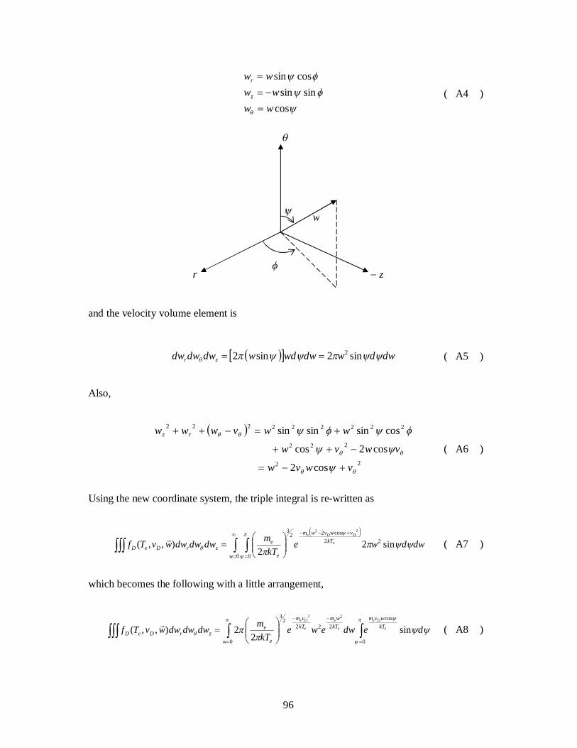
96
cossinsin
cossin
wwww
ww
z
r
( A4 )
and the velocity volume element is
dwdwdwwdwdwdwdw zr sin2sin2 2 ( A5 )
Also,
22
222
222222222
cos2
cos2cos
cossinsinsin
vwvw
vwvw
wwvwww rz
( A6 )
Using the new coordinate system, the triple integral is re-written as
0 0
22cos22
3
sin22
),,(22
w
kTvwvwm
e
ezrDeD dwdwe
kTmdwdwdwwvTf e
DDe
( A7 )
which becomes the following with a little arrangement,
0 0
cos222
23
sin2
2),,(22
w
kTwvm
kTwm
kTvm
e
ezrDeD dedwewe
kTmdwdwdwwvTf e
De
e
e
e
De
( A8 )
r
z
w
97
Now, let e
De
kTwvmt cos
and the last integral turns into
t
wvmkTddd
De
e cossin
e
De
e
Dee
De
e
De
e
De
kTwvm
kTwvm
De
ekT
wvm
kTwvm
t
De
ekTwvm
eewvm
kTdtewvm
kTde
0
cos
sin
( A9 )
Substitute Eq. A9 into Eq. A8 into to get
0
2222
3 22
22
),,(
w
kTwvm
kTwvm
De
ekTwm
kTvm
e
e
zrDeD
dweewvm
kTewekT
m
dwdwdwwvTf
e
De
e
De
e
e
e
De
( A10 )
By the definition of energy 2
21 wmE e , wdwmdE e and drift energy 2
21
DeD vmE , Eq.
A10 can be written with energy notations,
0
4
0
22
0
22
0
22
12
1
21
21
12
1
),,(
2
E
kTEE
kTEE
De
E
kTEEEE
kTEEEE
De
E
kTEEEE
kTDEEEE
De
E
kTEE
kTEE
D
kTE
kTE
e
zrDeD
dEeeEkT
dEeeEkT
dEeeEkT
dEeeE
eekT
dwdwdwwvTf
e
D
e
D
e
DD
e
DD
e
DD
e
D
e
D
e
D
ee
D
( A11 )
From the definition shown in Eq. A2, the EEDF in the energy space can be realized from Eq.
A11 as
98
e
D
e
D
kTEE
kTEE
DeDeD ee
EkTEETf
4
12
1),,(
2
( A12 )
which completes the derivation of Eq. A1.
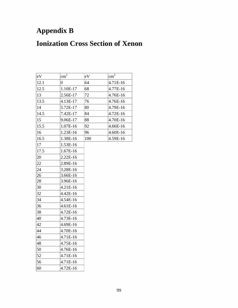
99
Appendix B
Ionization Cross Section of Xenon
eV cm2 eV cm2 12.1 0 64 4.71E-16 12.5 1.10E-17 68 4.77E-16 13 2.56E-17 72 4.76E-16 13.5 4.13E-17 76 4.76E-16 14 5.72E-17 80 4.79E-16 14.5 7.42E-17 84 4.72E-16 15 9.06E-17 88 4.70E-16 15.5 1.07E-16 92 4.66E-16 16 1.23E-16 96 4.60E-16 16.5 1.38E-16 100 4.59E-16 17 1.53E-16 17.5 1.67E-16 20 2.22E-16 22 2.89E-16 24 3.28E-16 26 3.66E-16 28 3.96E-16 30 4.21E-16 32 4.42E-16 34 4.54E-16 36 4.61E-16 38 4.72E-16 40 4.73E-16 42 4.69E-16 44 4.70E-16 46 4.71E-16 48 4.75E-16 50 4.76E-16 52 4.71E-16 56 4.71E-16 60 4.72E-16

100
Appendix C
Excitation Cross Section of Xenon
eV cm2 10 1.80E-17 10.5 2.40E-17 11 4.20E-17 11.5 6.20E-17 12 8.40E-17 12.5 1.05E-16 13 1.28E-16 14 1.70E-16 15 2.14E-16 16 2.55E-16 18 3.35E-16 20 3.73E-16 25 3.85E-16 30 3.57E-16 40 2.85E-16 50 2.40E-16 60 2.10E-16 70 1.85E-16 80 1.66E-16 90 1.52E-16 100 1.38E-16
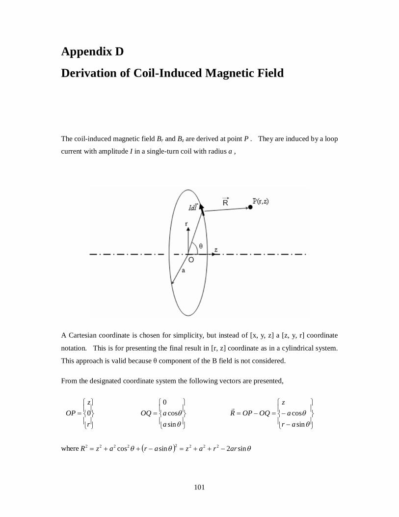
101
Appendix D
Derivation of Coil-Induced Magnetic Field
The coil-induced magnetic field Br and Bz are derived at point P . They are induced by a loop
current with amplitude I in a single-turn coil with radius a ,
A Cartesian coordinate is chosen for simplicity, but instead of [x, y, z] a [z, y, r] coordinate
notation. This is for presenting the final result in [r, z] coordinate as in a cylindrical system.
This approach is valid because θ component of the B field is not considered.
From the designated coordinate system the following vectors are presented,
r
zOP 0
sincos
0
aaOQ
sincosar
az
OQOPR
where sin2sincos 22222222 arrazarazR
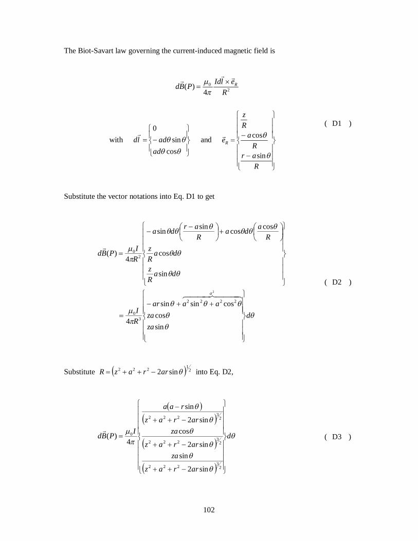
102
The Biot-Savart law governing the current-induced magnetic field is
2
0
4)(
RelIdPBd R
with
cossin
0
adadld
and
RarR
aRz
eR
sin
cos
( D1 )
Substitute the vector notations into Eq. D1 to get
dzaza
aaar
RI
daRz
daRz
Rada
Rarda
RIPBd
a
sincos
cossinsin
4
sin
cos
coscossinsin
4)(
2
2222
30
20
( D2 )
Substitute 21222 sin2 arrazR into Eq. D2,
d
arraz
zaarraz
zaarraz
raa
IPBd
23222
23222
23222
0
sin2
sinsin2
cossin2
sin
4)(
( D3 )

103
Integrate Eq. D3 to get
2
0
23222
23222
0
sin2
sin_
sin2
sin
4)()()(
)( d
arraz
zaconsiderednot
arraz
ra
Ia
PBPBPB
PB
r
y
z ( D4 )
note: 2
322221222 sin2
sin
sin2
1
arraz
ra
arraza
2
322221222 sin2sin2
1
arraz
z
arrazz
and the equations for Br and Bz are arrived,
2
2
21222
0
sin2
sin2
arraz
dz
IaBr ( D5 )
2
2
21222
0
sin22
arraz
da
IaBz ( D6 )
A limiting case can be checked for verification. For (r,z) = (0,0) at the axis of symmetry,
0rB and aIBz 2
0 (field induced by a long solenoid). Indeed,
aI
aIa
ad
aIaBz 2
122
02
02
2
00,0@
and the derivation is verified.

104
The analytic form of vector potential A
that satisfies AB
still needs to be found. Here
the only interest is in A from the axisymmetric assumption of the code. There are two ways
that A can be found as the curl of A
yields two equations: rBzA
and zBrA
rr
1 ;
and the former is chosen. To proceed, the equation of rB is first transformed into analytical
form. The procedure is as follows. Let
22
4
raz
arm
and
22
( D7 )
dmzraz
Ia
d
razarraz
zIaBr
2
02
2
220
2
0 222
22
20
sin1sin42
2
2sin41
sin212
( D8 )
Note: m
DmD
1sinsin1 22
22
2 sin1442sin1142sin42 mmmm
m
Rearrangement Eq. D8 to obtain
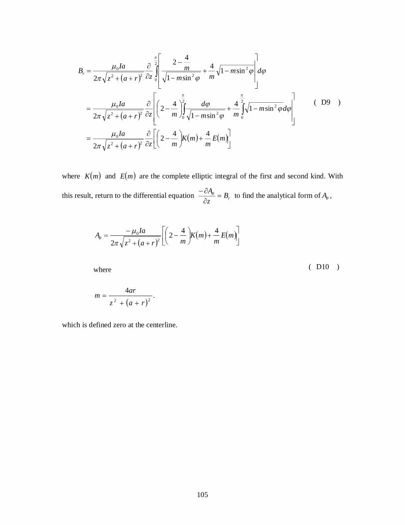
105
mEm
mKmzraz
Ia
dmmm
dmzraz
Ia
dmmm
mzraz
IaBr
4422
sin14sin1
422
sin14sin1
42
2
22
0
2
0
22
0222
0
2
0
2
222
0
( D9 )
where mK and mE are the complete elliptic integral of the first and second kind. With
this result, return to the differential equation rBzA
to find the analytical form of A ,
mE
mmK
mrazIaA 442
2 220
where
22
4
raz
arm
.
( D10 )
which is defined zero at the centerline.
106
References
1 Lozano, P., Glass B., Martinez-Sanchez M., “Performance Characteristics of a Linear Ionic Liquid Electrospray Thruster,” Proceedings of the 29th International Electric Propulsion Conference, Princeton, NJ, October 2005. IEPC-2005-192.
2 Hruby, V., et al, “ST7-DRS Colloid Thruster System Development and Performance Summary,” Proceedings of the 44th AIAA Joint Propulsion Conference, Hartford, CT, July 2008. AIAA-2008-4824.
3 Marcuccio, S., Paita, L., Saviozzi, M., Andrenucci, M., “Flight Demonstration of FEEP on Get Away Special,” Proceedings of the 34th AIAA Joint Propulsion Conference, Cleveland, OH, July 1998. AIAA-1998-3332.
4 Bassner, H., et al, “The ESA-XX Ion Thruster,” Proceedings of the 2nd European Spacecraft Propulsion Conference (ESA SP-398), Noordwijk, the Netherlands, May 1997. Paris: European Space Agency, 1997. p.251.
5 Goebel, D. and Katz, I., Fundamentals of Electric Propulsion: Ion and Hall Thrusters, New Jersey: Wiley, 2008. pp. 435-437.
6 Bassner, H., et al, “Application of the RF Ion Thruster RIT 10 to Stationkeeping of Geostationary Satellites and Primary Spacecraft Propulsion,” Proceedings of the 10th AIAA Electric Propulsion Conference, Lake Tahoe, NV, October 1973. AIAA-1973-1100.
7 Leiter, H., et al, “Evaluation of the Performance of the Advanced 200mN Radio Frequency Ion Thruster RIT-XT,” Proceedings of the 38th AIAA Joint Propulsion Conference, Indianapolis, IN, July 2002. AIAA-2002-3836.
8 Bassner, H., et al, “ Development Steps of the RF-Ion Thrusters RIT,” Proceedings of the 27th International. Electric Propulsion Conference, Pasadena, CA, October 2001. IEPC-01-105.
9 http://cs.space.eads.net/sp/SpacecraftPropulsion/Rita/RIT-10.html.
10 Tsay, M., Hohman, K. and Olson, L., “Micro RF Ion Engine for Small Satellite Applications,” Proceedings of the 23rd AIAA/USU Conference on Small Satellites, North Logan, UT, August 2009. SSC09-II-1.
11 Warner, N., “Theoretical and Experimental Investigation of Hall Thruster Miniaturization,” Doctoral Dissertation, Massachusetts Institute of Technology, Cambridge, MA, 2007.
12 Reichbach, J.G., Sedwick, R.J. and Martinez-Sanchez, M., “Micropropulsion System Selection for Precision Formation Flying Satellites,” Proceedings of the 37th AIAA Joint Propulsion Conference, Salt Lake City, UT, July 2001. AIAA-2001-3646.

107
13 van Put, P., van der List, M., and Yuce, V., ”Development of an Advanced Proportional
Xenon Feed Assembly for the GOCE Spacecraft,” Proceedings of the 4th International Spacecraft Propulsion Conference (ESA SP-555), Sardinia, Italy, June 2004. Published on CDROM., p.50.1.
14 Busek Brochure: Ion Thruster Systems.
15 Piejak, R., Godyak, V., and Alexandrovich, B., “A Simple Analysis of an Inductive RF Discharge,” Plasma Sources Science and Technology, Vol. 1, 1992. pp. 179-186.
16 Vahedi, V., et al, “Analytic Model of Power Deposition in Inductively Coupled Plasma Sources,” Journal of Applied Physics, Vol. 78, No. 3, 1995.
17 Lymberopoulos, D. and Economou, D., “Two-Dimensional Self-Consistent Radio Frequency Plasma Simulations Relevant to the Gaseous Electronics Conference RF Reference Cell,” Journal of Research of the National Institute of Standards and Technology, Vol. 100, No. 4, 1995. pp. 473-494.
18 Kumar, H., and Roy, S., “Two-Dimensional Fluid Model of DC and RF Plasma Discharges in Magnetic Field,” Proceedings to the 36th AIAA Plasma Dynamics and Laser Conference, Toronto, Canada, June 2005. AIAA-2005-4788.
19 Lee, S., Iza, F., and Lee, J., “Particle-in-Cell Monte Carlo and Fluid Simulations of Argon-Oxygen Plasma: Comparisons with Experiments and Validations,” Physics of Plasma, Vol 13, No. 5, 2006. pp. 057102.
20 Takekida, H., and Nanbu, K., “Self-Consistent Particle Modeling of Inductively Coupled CF4 Discharges and Radical Flow,” IEEE Transactions on Plasma Science, Vol. 34, No. 3, June 2006. pp. 973-983.
21 Oh, J., and Makabe, T., “A Numerical Study of a Collision-Dominated Inductively Coupled Plasma Using Particle-in-Cell/Monte Carlo Simulation,” Japanese Journal of Applied Physics, Vol. 38, 1999. pp. 4423-4428.
22 Froese, A., “Particle-in-Cell Simulations of Nonlocal and Nonlinear Effects in Inductively Coupled Plasmas,” S.M. Thesis, University of Saskatchewan, Saskatchewan, Canada, 2007.
23 Arzt, T., “Numerical Simulation of the RF Ion Source RIG-10,” Journal of Physics D: Applied Physics, Vol 21, 1988. pp. 278-285.
24 Mistoco, V., and Bilen, S., “Numerical Modeling of a Miniature Radio-Frequency Ion Thruster,” Proceedings to the 44th AIAA Joint Propulsion Conference, Hartford, CT, July 2008. AIAA-2008-5194.
25 Closs, M., “RF Ion Thruster Design Software Based on Numerical Modeling,” Proceedings to the 3rd International Conference on Spacecraft Propulsion, Cannes, France, October 2000. 2000ESASP.465.419C.

108
26 Chen, G., and Raja, L., “Fluid Modeling of Electron Heating in Low-Pressure,
High-Frequency Capacitively Coupled Plasma Discharges,” Journal of Applied Physics, Vol. 96, No. 11, 2004. pp. 6073-6081.
27 Mikellides, I., Katz, I., Goebel, D., Polk, J., “Hollow cathode theory and experiment. II. A two-dimensional theoretical model of the emitter region”, Journal of Applied Physics Vol. 98, No. 11, 2005, pp. 113303.
28 Szabo, J., Martinez-Sanchez, M. and Batishchev, O., “Fully Kinetic Hall Thruster Modeling”, Proceedings to the 27th International Electric Propulsion Conference, Pasadena, CA, October 2001. IEPC-01-341.
29 Zhao, S., et al, “Fluid Simulation of the E-H Mode Transition in Inductively Coupled Plasma,” Journal of Applied Physics, Vol 105, No. 8, 2009. pp. 083306.
30 Farnell, C., “Performance and Lifetime Simulation of Ion Thruster Optics,” Doctoral Dissertation, Colorado State University, Fort Collins, Co, 2007.
31 Ye, R and Ishigaki, T., “Modeling of Transient Nonequilibrium Phenomena in an Inductively Coupled Plasma under Pulsed Power Conditions,” Journal of Applied Physics, Vol. 97, No. 12, 2005, pp. 123306.
32 Tsay, M. and Martinez-Sanchez, M., “Simple Performance Modeling of a Radio-Frequency Ion Thruster,” Proceedings to the 30th International Electric Propulsion Conference, Florence, Italy, September 2007. IEPC-2007-072.
33 Tsay, M. and Martinez-Sanchez, M., “Two-Dimensional Simulation of a Radio-Frequency Ion Thruster Discharge,” 44th AIAA/ASME/SAE/ASEE Joint Propulsion Conference and Exhibit, Hartford, CT, July 2008, AIAA-2008-5196
34 Tsay, M., “Numerical Modeling of a Radio-Frequency Micro Ion Thruster,” S.M. Thesis, Massachusetts Institute of Technology, Cambridge, MA, 2006.
35 Grover, F.W., Inductance Calculations, Working Formulas and Tables, D. Van Norstrand Company, Inc., NY, 1946. pp. 114-115, 143.
36 Fridman, A. and Kennedy, L.A., Plasma Physics and Engineering, Taylor & Francis Books, Inc., 2004. pp. 195-196 & 336.
37 Gans, T., Schultz-von der Gathen, V., and Dobele, H., “Spectroscopic Measurements of Phase-Resolved Electron Energy Distribution Function in RF-Excited Discharges,” Europhysics Letters, Vol. 66, No. 2, 2004. pp-232-238.
38 Szabo, J., “Fully Kinetic Numerical Modeling of a Plasma Thruster,” Ph.D. dissertation,
Massachusetts Institute of Technology, Cambridge, MA, 2001. 39 Crispel, P., Degand, C., and Vignal, M., “An Asymptotic Preserving Scheme for the
Two-Fluid Euler-Poisson Model in the Quasi-Neutral Limit,” Journal of Computational Physics, Vo. 223, No. 1, 2007. pp. 208-234.
109
40 Lieberman, M.A. and Lichtenberg, A.J., Principles of Plasma Discharges and Materials Processing, John Wiley & Sons, Inc., New York, 1994. pp. 39.
41 Parra, F., Ahedo, E., Fife, M. and Martinez-Sanchez, M., “A Two-Dimensional Hybrid Model of the Hall thruster Discharge,” Journal of Applied Physics, Vol. 100, No.2, 2006. pp. 023304.
42 Horst, L., et al, “Development of a RIT-Millithruster,” Proceedings to the 55th International Astronautical Congress, Vancouver, Canada, October 2004. IAC-04-S.4.04.