two-dimensional natural element analysis of double · pdf filetwo-dimensional natural element...

Two-dimensional natural element analysis ofdouble-free surface flow under a radial gate

Farhang Daneshmand, S.A. Samad Javanmard, Jan F. Adamowski,Tahereh Liaghat, and Mohammad Mohsen Moshksar

Abstract: The gravity-driven free surface flow problems for which both the solid and free surface boundaries are highlycurved are very difficult to solve. A computational scheme using a variable domain and a fixed domain natural elementmethod (NEM) is developed in the present study for the computation of the free surface profile, velocity and pressure distri-butions, and the flow rate of a 2D gravity fluid flow through a conduit and under a radial gate. The problem involves twohighly curved unknown free surfaces and arbitrary curved-shaped boundaries. These features make the problem more com-plicated than flow under a sluice gate or over a weir. The fluid is assumed to be inviscid and incompressible and the resultsobtained are confirmed by conducting a hydraulic model test. The results are in agreement with other flow solutions for freesurface profiles and pressure distributions.

Key words: free surface flow, natural neighbour interpolation, numerical methods, hydraulic gates.

Résumé : Les problèmes d’écoulement gravitaire en surface libre où les limites imposées par les parois solides et la surfacelibre sont très courbes sont très difficiles à résoudre. Un modèle informatique utilisant une méthode d’éléments naturels àdomaine variable et à domaine fixe est développée dans la présente étude afin de calculer le profil de la surface libre, lesdistributions de vitesse et de pression ainsi que le débit d’un écoulement gravitaire bidimensionnel d’un fluide dans unconduit et sous une vanne à segment. Le problème implique deux surfaces libres inconnues très courbées et des limitescourbes arbitraires. Ces caractéristiques rendent le problème plus compliqué que celui de l’écoulement sous une vanne regis-tre ou par-dessus un déversoir. Il est présumé que le fluide est incompressible et non visqueux; les résultats obtenus sontconfirmés par un essai utilisant un modèle hydraulique. Les résultats concordent avec les autres solutions d’écoulement pourles profiles à surface libre et les distributions de pression.

Mots‐clés : écoulement en surface libre, interpolation du voisin naturel, méthodes numériques, écluses hydrauliques.

[Traduit par la Rédaction]

Introduction

Various types of hydraulic structures are commonly usedin rivers and channels as control structures. Examples ofthese control structures include spillways, weirs, and varioustypes of gates. The fluid loads on such structures and the freesurface profiles of the flow have to be determined for designpurposes. This is a difficult task because the determination ofthe free surface location as a part of the solution involves thesolution of an intrinsically nonlinear problem. Neither the lo-cation of the free surface nor the magnitude of the flow dis-charge is known a priori and to date, no exact solutions havebeen proposed. Using analytical methods such as conformalmapping for solving the problem are limited in number dueto the necessity to establish certain mapping relations andthe difficulty in satisfying the nonlinear boundary conditionof constant pressure along the free surface. Moreover, the

nonlinear nature of the problem dictates a numerical solutionprocedure at the end of such analysis (Larock 1970; Petrila2002).Among the many numerical methods, the finite element

method (FEM) (Ikegawa and Washizu 1973; Chan et al.1973; Bettess and Bettess 1983; Abdel-Malek et al. 1989;Sankaranarayanan and Rao 1996; Daneshmand et al. 2000)and the boundary-element method (Cheng et al. 1981) havegained popularity. Most of these methods have been success-fully applied to the cases of flows over spillways or undersluice gates with only one free surface and a simple geome-try. Regarding the difficulty associated with remeshing inFEM, the past decade has seen a tremendous surge in the de-velopment of a family of Galerkin and collocation based nu-merical methods known as meshless methods (Belytschko etal. 1994; Liu et al. 1995; Daneshmand and Niroomandi2007). The natural element method (NEM) is a Galerkin

Received 3 June 2011. Revision accepted 10 April 2012. Published at www.nrcresearchpress.com/cjce on 28 May 2012.

F. Daneshmand and J.F. Adamowski. Department of Bioresource Engineering, Faculty of Agricultural and Environmental Sciences,McGill University, 21111 Lakeshore Road, Ste. Anne de Bellevue, QC H9X 3V9, Canada.S.A.S. Javanmard and M.M. Moshksar. Mechanical Engineering Department, Marvdasht Branch, Islamic Azad University, Marvdasht,Iran.T. Liaghat. Mechanical Engineering Department, École Polytechnique de Montréal, P.O. Box 6000, Montréal, QC H3C 3A7, Canada.

Corresponding author: Farhang Daneshmand (e-mail: [email protected]).

Written discussion of this article is welcomed and will be received by the Editor until 31 October 2012.

643

Can. J. Civ. Eng. 39: 643–653 (2012) doi:10.1139/L2012-046 Published by NRC Research Press

Can

. J. C

iv. E

ng. D

ownl

oade

d fr

om w

ww

.nrc

rese

arch

pres

s.co

m b

y M

CG

ILL

UN

IVE

RSI

TY

on

10/0

5/13

For

pers

onal

use

onl

y.

based method that is built upon Voronoi diagrams and Delau-nay tessellations (Sukumar et al. 2001). This interpolationscheme has several very useful properties, such as its strictlyinterpolating character, its ability to exactly interpolate piece-wise linear boundary conditions, and a well-defined and ro-bust approximation with no user-defined parameter on non-uniform grids. Yvonnet et al. (2004) provided a detailed re-view on natural neighbour interpolation and its drawbacks innon-convex domains. González et al. (2007) presented a nat-ural neighbour Galerkin method in conjunction with a-shapesfor the numerical simulation of free-surface dynamics offlows within an updated Lagrangian treatment. Recently, Da-neshmand et al. (2010) presented a numerical procedurebased on natural element discretization that treats the fluidflow through a sluice gate with a free surface.Despite some progress in solving gravity driven free sur-

face flows with various numerical methods, solving the prob-lem with two highly curved free surfaces via the use of NEMhas not been investigated. Fluid flows that are driven bygravity and in which the solid and free surface boundariesare highly curved are considerably more complicated. Suchsituations occur, for instance, in the case of flow under a ra-dial gate placed at the end of a conduit. In this case, a largeextent of the free water jet downstream of the gate has to beconsidered in determining the pressure distribution along thegate. In addition to these characteristics, the free jet flow hastwo unknown free surfaces to be determined and is thereforemore difficult to manage. Our aim is to present a numericalprocedure based on natural element discretization that treatsthe fluid flow through a gate with two highly curved free sur-faces and arbitrary shaped boundaries. The novel features ofthe present study are that (1) it involves two free surfaces and(2) the free surfaces are relatively long and have a morecurved shape than the flow under a sluice gate or over aspillway. In the present study, lower and upper free surfaceprofiles, velocity and pressure distributions, and flow rateper unit width Q are calculated for a known Bernoulli con-stant, B, using the natural element method. Results for pres-sure distribution are compared with measured valuesobtained by conducting a hydraulic model test.

Problem formulation and discretization

Flows under radial gates can be considered as rapidly con-verging flows in which the influence of fluid viscosity is quitesmall in comparison with interial effects, and consequently, inalmost all studies of problems of this type, we can assumethat the flow is irrotational. A typical two-dimensional steadyflow from a reservoir, through an arbitrary shaped conduitand under a radial gate in the pattern of a free jet is shown inFig. 1. Geometry of the conduit walls S2 and S7 are given andthe far upstream and downstream boundaries of the flow do-main, denoted by S1 and S4 are assumed to be normal andperpendicular to the flow direction, respectively. The boun-dary S6 is the surface of the radial gate and can be consideredas a fixed solid boundary. The lower and upper free surfaceprofiles S3 and S5 are not known a priori. Either, the flow dis-charge per unit width of conduit is given and the stagnationlevel and flow field are sought, or the stagnation level isgiven and the corresponding rate of flow per unit width ofchannel is to be determined. In the present study, the flowrate Q is assumed to be unknown and the stagnation level isgiven as HE, which is the stagnant fluid level above point A.For convenience, the origin of the coordinate system is lo-cated as shown in Fig. 1. The horizontal and vertical coordi-nates are denoted by x and y, respectively.For the two-dimensional potential flow, the flow velocities

vx and vy is defined in terms of a stream function (j)

½1� vx ¼ j;y vy ¼ �j;x

and the flow is governed by the Laplace equation,

½2� j;xx þ j;yy ¼ 0 onU

where j is the stream function, U is the flow domainbounded by the aforementioned boundaries, and comma de-notes differentiation. The numerical solution of partial differ-ential eq. [2] requires some form of spatial discretization.Basically, there are two different types of specification forthe flow field, Lagrangian and Eulerian. We can think of theLagrangian mesh as being drawn on the body. The mesh de-

Fig. 1. Fluid flow through a conduit and under the radial gate.

644 Can. J. Civ. Eng. Vol. 39, 2012

Published by NRC Research Press

Can

. J. C

iv. E

ng. D

ownl

oade

d fr

om w

ww

.nrc

rese

arch

pres

s.co

m b

y M

CG

ILL

UN

IVE

RSI

TY

on

10/0

5/13

For

pers

onal

use

onl

y.

forms with the body and both the nodes and the materialpoints change position as the body deforms. However, theposition of the material points relative to the nodes remainsfixed. On the other hand, the Eulerian mesh is a backgroundmesh. The body flows through the mesh as it deforms. Thenodes remain fixed and the material points move through themesh. The position of a material point relative to the nodesvaries with the motion. The natural element method which isbased on the Lagrangian approach is used in the presentstudy. As the first step in the numerical solution, the problemdomain is divided into elements with a suitable interpolationmodel assumed for j(e) as

½3� jðeÞðx; yÞ ¼Xmi¼1

4iðx; yÞjðeÞi

where 4i(x, y) is the natural element interpolation function asgiven in the next section and m is the number of neighbor-hoods of point (x, y).The boundary conditions of the problem are

½4� j ¼ 0 on S2 and S3

½5� j ¼ Q on S5; S6 and S7

½6� j;n ¼ �ffiffiffiffiffiffiffi2gz

pon S3 and S5

½7� j;n ¼ 0 on S1 and S4

It should be noted that for the purposes of the numericalsolution, outflow streams are cut at right angles to the pri-mary velocity. Boundary condition eq. [7] is applied on thispart, which means that there is no velocity normal to themain flow. Here, n is the outward normal to the boundary, zis the distance of the free surface from the datum line of the

stagnation level, and g is the gravitational acceleration. Theproblem is to find the corresponding upper and lower freesurface profile, together with the velocity field, in particularthe pressure distribution on the gate by solving eq. [2] sub-ject to the boundary conditions eqs. [4]–[7], given either thetotal head HE or the flow rate Q. In the present study, HE isgiven and Q is found as part of the solution.

Voronoi diagrams and Delaunay tessellations

Classical definitions for Voronoi diagrams and Delaunaytessellations as used in NEM can be found in Yvonnet et al.(2004) and González et al. (2007). The first-order Voronoidiagram of the set N = {n1, n2, …, nM} is a sub-division ofthe space into regions TI, such that any point in TI is closer tonI than to any other node of the set. The region TI is the Vor-onoi cell of nI and is defined as

½8� TI ¼ fx 2 R2 : dðx; xIÞ < dðx; xJÞ 8J 6¼ Igwhere d(xI, xJ) is the Euclidean distance between xI and xJ.The Delaunay tessellation is constructed by connecting nodeswhose Voronoi cells have common boundaries (Fig. 2a). Animportant property of Delaunay triangles is that the circumcir-cle of any Delaunay triangle of the nodal set N contains noother nodes of N. Introduction of a point X into the problemdomain U, the Voronoi cells for the point X and its naturalneighbours are shown in Fig. 2b (Cueto et al. 2003). In thissection, Sibson and non-Sibsonian (Laplace) interpolationschemes (Sukumar et al. 1998; Sukumar and Moran 1999;Cueto et al. 2003) are reviewed, although only Sibson inter-polation will be used in the examples included in this paper.For the Sibson shape functions the natural neighbour coor-

dinates of x are defined as the ratio of the area of overlap oftheir Voronoi cells to the total area of the Voronoi cell of x(Fig. 2a),

Fig. 2. Definition of the natural neighbour coordinates in NEM: (a) original Voronoi diagram and (b) first-order and second-order Voronoicells about x (modified from Cueto et al. 2003).

Daneshmand et al. 645


Can

. J. C

iv. E

ng. D

ownl

oade

d fr

om w

ww

.nrc

rese

arch

pres

s.co

m b

y M

CG

ILL

UN

IVE

RSI

TY

on

10/0

5/13

For

pers

onal

use

onl

y.

½9� FIðxÞ ¼ AIðxÞAðxÞ

The first derivatives of the shape functions are

½10� FI;jðxÞ ¼ AI;jðxÞ �FIðxÞA;jðxÞAðxÞ ðj ¼ 1; 2Þ

In two dimensions, the non-Sibsonian shape function FI(x)takes the form

½11� FIðxÞ ¼ aIðxÞXnJ¼1

aJðxÞaJðxÞ ¼ sJðxÞ

hJðxÞ

where sI(x) is the length of the Voronoi edge associated withnode I and hI(x) is the perpendicular distance between theVoronoi edge of node I to x (Fig. 3). The derivative of thenon-Sibsonian shape function is obtained by differentiatingeq. [11] as

½12� FI;jðxÞ ¼ aI;jðxÞ �FIðxÞa;jðxÞXJ

aJðxÞðj ¼ 1; 2Þ

Multiplying the governing eq. [2] by 4i selected accordingto the Galerkin approach, we get

½13�ZZUðeÞ

4i

�jðeÞ;xx þ jðeÞ

;yy

�dU ¼

ZZUðeÞ

4i

�4i;xj

ðeÞ;x þ 4i;yj

ðeÞ;y

�dU�

ZG ðeÞ

4i

�jðeÞ;x nx þ jðeÞ

;y ny

�dG ¼ 0

where U(e) and G(e) denote the domain and boundary of ele-ment (e), respectively. Using the integration by-parts andboundary conditions given in eqs. [4] to [7] and the proce-dure given in Daneshmand et al. (2010), the discretizedform of eq. [13] leads to the following system of equationsin matrix form:

½14� Kj ¼ P

where K is the total system matrix for the problem, j is thevector including the unknown nodal values of the streamfunction, and P is the total load vector. It should be notedthat the system matrices K and P are obtained by assemblingthe following element matrices:

½15� KðeÞ ¼ZZA

BTBdA B ¼41;x 42;x ::: 4m;x

41;y 42;y ::: 4m;y

" #

½16� PðeÞ ¼ �ZG

V0NTdG NT ¼ 41 42 . . . 4m

h i

where A and G are the area and boundary of an element,respectively.

Iteration for the free surfaces

The constant pressure condition on the upper and lowerfree surfaces requires

½17� 1

2g

@j

@n

� �2

þ y ¼ B

where y is the free surface elevation, g is the gravity accelera-tion, and B is the Bernoulli constant. When the Bernoulliconstant, B, is known, the problem is first solved by assum-ing the location of the free surfaces and applying the bound-ary conditions, eqs. [4]–[7]. The solution yields differentvalues of the stream function at each of the free surfacenodes. If the stream function is constant for all points on thefree surfaces, the problem is solved; otherwise, an iterationscheme must be used to adjust the free surface elevation.The calculated value of the stream function jk at the startpoint of the free surface is considered as a good estimationfor Qk+1 to perform the free surface adjustment in the nextiteration. The x and y-components of the velocity for free sur-face nodes are calculated by using equation eq. [1]. By satis-fying the zero normal velocity condition on the free surfaces,the free surface correction can be achieved by using the fol-lowing relations (Fig. 4) (Daneshmand et al. 2000):

Fig. 3. Construction of non-Sibsonian interpolants (modified fromSukumar et al. 2001).

Fig. 4. Node adjustment.

646 Can. J. Civ. Eng. Vol. 39, 2012


Can

. J. C

iv. E

ng. D

ownl

oade

d fr

om w

ww

.nrc

rese

arch

pres

s.co

m b

y M

CG

ILL

UN

IVE

RSI

TY

on

10/0

5/13

For

pers

onal

use

onl

y.

½18�Dy� ¼ bDx

6ða1 þ a2 þ a3Þ whenDy > 0

Dy� ¼ Dx

6bða1 þ a2 þ a3Þ whenDy < 0

8>><>>:

where b is the correction factor for the free surface and a1,a2, and a3 are the slopes of the velocities at three successivenodes on the free surface and can easily be obtained by usingtheir x and y-velocity components.Although it is theoretically possible to assume the location

of both the lower and the upper free surfaces, test calcula-tions of this kind have proven to be time consuming withconvergence problems. Instead, an alternating iterative proce-dure is used in this study. The lower and upper free surfacesare approximated in the first iteration. Then the lower freesurface location is kept fixed while the upper free surface isallowed to vary. The same procedure is repeated until boththe lower and the upper free surfaces converge with a speci-fied accuracy. According to this procedure, the computer im-plementation of the present numerical procedure includes thefollowing steps:Step 1. As shown in Fig. 5, the initial problem domain is

divided into fixed and variable domains. In the fixed domain,all nodes are active whereas node activation depends on thenode positions in the variable domain.Step 2. The initial trial upper and lower free surface pro-

files are assumed.Step 3. The lower free surface profile is assumed to be

fixed. Dirichlet and Neumann boundary conditions are ap-plied to the nodes on the lower and upper free surface pro-files, respectively. Moreover, the number of neighborhoodsfor any point of a triangular element in FEM is three whereasthe number of neighborhoods in NEM can be greater thanthree. For three typical points of a triangular element asa(x1, y1), b(x2 ,y2), and c(x3, y3), matrix B is evaluated by us-ing eq. [15] as

½19� B ¼ 1

2AðeÞy2 � y3 y3 � y1 y1 � y2

x3 � x2 x1 � x3 x2 � x1

" #

where A(e) is the element area. It is necessary to use a suita-ble algorithm for finding the shape functions and their deri-vatives for evaluating matrix B.Step 4. The problem is solved using the proposed method

and the values of the stream function (j) for all nodes arecalculated as a function of the assumed upper free surfaceprofile. The flow rate Qkþ1

upper can then be calculated and theupper free surface is corrected by eq. [18]. The iterationprocess is continued until the maximum value of the conver-gence criterion defined as jQkþ1 � jk

i j=Qkþ1 is less than aprescribed accuracy 3 (for upper free surface).Step 5. The upper free surface profile is assumed to be

fixed and Dirichlet and Neumann boundary conditions areapplied to the nodes on the upper and lower free surfaces, re-spectively.Step 6. The problem is solved and the value of discharge

(j) is calculated for all nodes as a function of the assumedlower free surface profile. The flow rate Qkþ1

lower can be calcu-lated and the lower surface is corrected according to eq. [18].The iteration process is continued until the maximum valueof the convergence criterion defined as jQkþ1 � jk

i j=Qkþ1 isless than a prescribed accuracy 3 (for lower free surface).Step 7. The above steps (3 to 6) are repeated until a pre-

Fig. 5. Active and inactive nodes in fixed and variable domain.

Table 1. Karun-III dam specifications (example 1).

Type of dam Arch concrete damHeight (from the river bed) 205 mLength 462 mBase width 29.5 mSpillway capacity 15 000 m3/sReservoir capacity 2 970 000 000 m3

Surface area 48 km2



Can

. J. C

iv. E

ng. D

ownl

oade

d fr

om w

ww

.nrc

rese

arch

pres

s.co

m b

y M

CG

ILL

UN

IVE

RSI

TY

on

10/0

5/13

For

pers

onal

use

onl

y.

scribed error criterion is satisfied on the differences in coor-dinates of all free surface nodes between successive itera-tions; that is

½20� jyri � yr�1i j � d for i ¼ 1; . . . ;Ns

where yri and yr�1i are y-coordinates of node i on the free sur-

face at iterations r and r–1, respectively; Ns is the number offree surface nodes; and d is the prescribed accuracy for nodespositions.

ResultsThe numerical procedure described above was applied to

flow under radial gates in two different cases. For both exam-ples, the results of the present study were compared withthose obtained from a hydraulic model test.

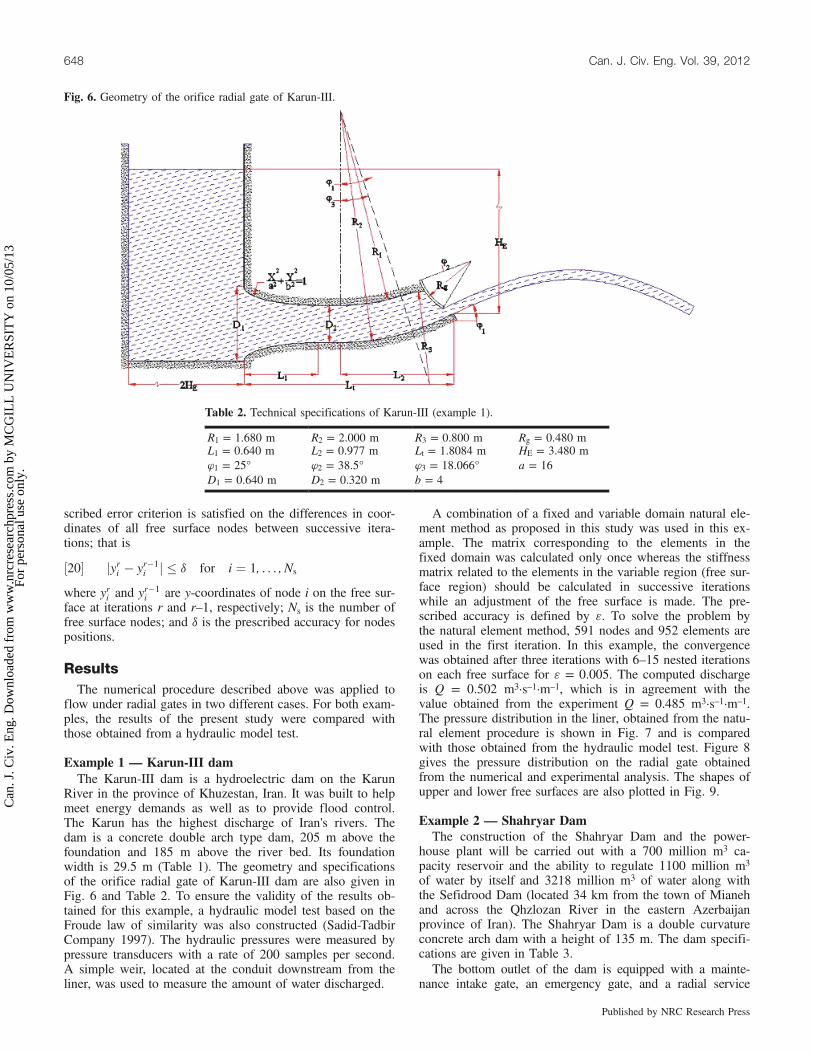
Example 1 — Karun-III damThe Karun-III dam is a hydroelectric dam on the Karun

River in the province of Khuzestan, Iran. It was built to helpmeet energy demands as well as to provide flood control.The Karun has the highest discharge of Iran's rivers. Thedam is a concrete double arch type dam, 205 m above thefoundation and 185 m above the river bed. Its foundationwidth is 29.5 m (Table 1). The geometry and specificationsof the orifice radial gate of Karun-III dam are also given inFig. 6 and Table 2. To ensure the validity of the results ob-tained for this example, a hydraulic model test based on theFroude law of similarity was also constructed (Sadid-TadbirCompany 1997). The hydraulic pressures were measured bypressure transducers with a rate of 200 samples per second.A simple weir, located at the conduit downstream from theliner, was used to measure the amount of water discharged.

A combination of a fixed and variable domain natural ele-ment method as proposed in this study was used in this ex-ample. The matrix corresponding to the elements in thefixed domain was calculated only once whereas the stiffnessmatrix related to the elements in the variable region (free sur-face region) should be calculated in successive iterationswhile an adjustment of the free surface is made. The pre-scribed accuracy is defined by 3. To solve the problem bythe natural element method, 591 nodes and 952 elements areused in the first iteration. In this example, the convergencewas obtained after three iterations with 6–15 nested iterationson each free surface for 3 = 0.005. The computed dischargeis Q = 0.502 m3·s–1·m–1, which is in agreement with thevalue obtained from the experiment Q = 0.485 m3·s–1·m–1.The pressure distribution in the liner, obtained from the natu-ral element procedure is shown in Fig. 7 and is comparedwith those obtained from the hydraulic model test. Figure 8gives the pressure distribution on the radial gate obtainedfrom the numerical and experimental analysis. The shapes ofupper and lower free surfaces are also plotted in Fig. 9.

Example 2 — Shahryar DamThe construction of the Shahryar Dam and the power-

house plant will be carried out with a 700 million m3 ca-pacity reservoir and the ability to regulate 1100 million m3

of water by itself and 3218 million m3 of water along withthe Sefidrood Dam (located 34 km from the town of Mianehand across the Qhzlozan River in the eastern Azerbaijanprovince of Iran). The Shahryar Dam is a double curvatureconcrete arch dam with a height of 135 m. The dam specifi-cations are given in Table 3.The bottom outlet of the dam is equipped with a mainte-

nance intake gate, an emergency gate, and a radial service

Table 2. Technical specifications of Karun-III (example 1).

R1 = 1.680 m R2 = 2.000 m R3 = 0.800 m Rg = 0.480 mL1 = 0.640 m L2 = 0.977 m Lt = 1.8084 m HE = 3.480 m41 = 25° 42 = 38.5° 43 = 18.066° a = 16D1 = 0.640 m D2 = 0.320 m b = 4

Fig. 6. Geometry of the orifice radial gate of Karun-III.

648 Can. J. Civ. Eng. Vol. 39, 2012


Can

. J. C

iv. E

ng. D

ownl

oade

d fr

om w

ww

.nrc

rese

arch

pres

s.co

m b

y M

CG

ILL

UN

IVE

RSI

TY

on

10/0

5/13

For

pers

onal

use

onl

y.

gate (Table 4). The maintenance gate is used for maintenancework of downstream equipment and is operated under the bal-anced pressure condition attained by means of a by-pass valvein the gate leaf. The service gate of the outlet is a radial gate.The definition sketch and technical specifications of the radialservice gate are given in Fig. 10 and Table 5, respectively.The value of head loss was calculated using the procedure

given in Roberson and Clayton (1997) for the entrance loss(loss coefficient = 0.03) and Brno Technical University(1994) for the outlet loss due to sudden contraction, respec-tively. To ensure the validity of the results obtained in this ex-

ample, a hydraulic model test (scale 1:15) based on Froude’slaw of similarity was also constructed (Shiraz University2007). The hydraulic model test included the entire passage ofwater both upstream and downstream of the gate. The hy-

Table 3. Shahryar Dam specifications (example 2).

Parameter Value (description)Type Double-arch concrete damHeight (from the river bed) 135 mCrest elevation 1045 m.a.s.l.Bottom outlet sill elevation 1004 m.a.s.l.Total storage (at normal water level) 700 MCMNormal water level 1035 m.a.s.l.Maximum water level 1041 m.a.s.l.

Note: m.a.s.l. is metres above sea level.

Table 4. Specifications of the bottom outlet gates (example 2).

Radial gateType Radial gateDischarge at normal water level 250 m3/sRadius 5.2 mWidth 3.8 mOpening 3 × 4 m (w × h)Maneuvering speed 0.3 m/minSealing type Rubber seal

Maintenance gateType Fixed wheel gateDimensions 3.85 × 6.2 m (w × h)Corrosion 2 mmBed elevation 1005.75 m

Emergency gateType Roller gateDischarge at normal water level 250 m3/sDimensions (gate/opening) 3.0 × 4.2 m (w × h)Maneuvering speed 0.3 m/minSealing type double stem rubber seal

Fig. 8. Pressure distribution on the radial gate (example 1).

Fig. 7. Pressure distribution on conduit walls (example 1).

Table 5. Technical specification for radial gate (example 2).

Parameter Value Parameter Valuea 1.15 i 0.167b 0.08 h 2.5c 0.44 R1 1d 0.71 R2 1.33e 0.55 Rg 0.347f 1.5 q 10°g 2.4 b 163°

Table 6. Dependence of the algorithm to the initializationstep (example 2).

Lower free surface profile (Fig. 13) Number of iterations1 1052 933 814 705 536 46



Can

. J. C

iv. E

ng. D

ownl

oade

d fr

om w

ww

.nrc

rese

arch

pres

s.co

m b

y M

CG

ILL

UN

IVE

RSI

TY

on

10/0

5/13

For

pers

onal

use

onl

y.

Fig. 10. Bottom-outlet radial service gate of Shahryar Dam (example 2).

Fig. 9. The shapes of the upper and lower free surfaces (example 2).

Fig. 11. Test stand for hydraulic model test (example 2).

650 Can. J. Civ. Eng. Vol. 39, 2012


Can

. J. C

iv. E

ng. D

ownl

oade

d fr

om w

ww

.nrc

rese

arch

pres

s.co

m b

y M

CG

ILL

UN

IVE

RSI

TY

on

10/0

5/13

For

pers

onal

use

onl

y.

Fig. 12. Locations of pressure measuring points (example 2).

Fig. 13. Free surface profile for radial gate opening 30% (example 2).

Table 7. Comparison between numerical and experimental results (example 2).

Mano. No. x (m) y (m) p (mH2O) model test p (mH2O) NEM Error (%) j (m3/s) NEM v (m/s) NEM1 1.4481 0.2643 2.2033 2.1658 1.7 0.2123 0.84612 1.4400 0.5250 1.9060 1.8835 1.2 0.4492 1.06783 1.0280 0.4332 2.0033 1.9665 1.9 0.4473 1.14624 0.7870 0.0364 2.3660 2.3506 0.7 0.0017 1.25005 0.7875 0.2107 2.2080 2.1778 1.4 0.2179 1.23886 0.4875 0.1752 2.2147 2.2016 0.6 0.2144 1.32827 0.4875 0.3401 2.0593 2.0404 0.9 0.4286 1.30088 0.1675 0.0697 2.2513 2.1930 2.7 0.1447 1.99869 0.1675 0.1397 2.1620 2.1805 0.8 0.2648 1.6905

10 0.1675 0.2093 2.1373 2.1725 1.6 0.3548 1.284011 0.2146 0.0250 2.3420 2.2757 2.9 0.0447 1.803912 0.2159 0.1430 2.2293 2.2053 1.1 0.2397 1.522413 0.2146 0.2620 2.1013 2.1355 1.6 0.3899 1.163314 0.1675 0.0360 2.2973 2.2051 4.2 0.0762 2.099515 0.1675 0.1058 2.1880 2.1862 0.1 0.2094 1.846416 0.1675 0.1750 2.1473 2.1805 1.5 0.3130 1.468717 0.1211 0.1390 2.2173 2.1369 3.8 0.3046 1.922018 0.1211 0.2570 2.1893 2.1769 0.6 0.4236 0.799819 0.1125 0.2768 2.1740 2.1711 0.1 0.4385 0.5938



Can

. J. C

iv. E

ng. D

ownl

oade

d fr

om w

ww

.nrc

rese

arch

pres

s.co

m b

y M

CG

ILL

UN

IVE

RSI

TY

on

10/0

5/13

For

pers

onal

use

onl

y.

draulic model was constructed using plexiglass material to se-cure good flow visualization. For better visualization of thefree surface profile, the downstream wall of the model wasmeshed by squares 5 cm × 5 cm. The test stand included threecentrifugal pumps, as well as main water storage and relevantchannels to complete the closed loop circuit (Fig. 11).For measuring pressure, manometers were installed at dif-

ferent points in the channel and a skin plate was positionedon the gate. The locations of pressure measuring points areshown in Fig. 12. The unit of measured pressure is mH2O.Water discharge was also measured by using the area–veloc-ity flow meter (Greyline AVFM-II). Its ultrasonic sensor wasinstalled at the bottom of the downstream channel. Based onthe speed of sound in the water, the level was measured withan accuracy of ±0.25%. Flow velocity was also measuredwith an ultrasonic Doppler signal. The instrument measuresvelocity with an accuracy of ±0.2%.The radial gate is considered to be in a 30% opening posi-

tion and the natural element method with 855 nodes and 1328elements (in the first iteration) was used to solve the problem.The discretization was made finer in the vicinity of the gate totake care of the higher velocity gradients in that region. Inthis example, the convergence was obtained on the free sur-face profiles with a prescribed accuracy 3 = 0.001. Two val-ues for the correction factor for lower and upper free surfacesare used in the calculations as bL = 1.20 and bU = 1.5, re-spectively. The computed discharge Q is 0.421 m3·m–1·s–1,which is in good agreement with the value obtained from theexperiment (Q = 0.399 m3·m–1·s–1). The pressure values aregiven in Table 6 and compared with the pressure values meas-ured in the hydraulic model test. The shape of the free surfa-

ces obtained from NEM is presented in Fig. 13. To study thedependence of the proposed algorithm to the initializationstep, we re-analyzed the problem with different lower free sur-face trials when keeping the upper free surface fixed. Asshown in Table 6 and Fig. 13, the algorithm converged forall cases with reasonable accuracy (3 = 0.005) and the num-ber of iterations decreased when the initial lower free surfaceprofile changed from 1 to 6, as expected. As can be seen fromTable 6, the pressure obtained from NEM is in agreementwith that obtained from the model test. It should also be notedfrom Table 7 that the maximum error in pressure values is2.9%. Figures 14 and 15 show the j and velocity contours,respectively.

ConclusionsHydraulic structures are used to regulate the flow of water

through canals and analysis of flows with free surfaces underhydraulic gates has received a good deal of attention in thefield of hydraulic engineering. Our aim in this paper was topresent a numerical procedure based on the natural elementmethod to treat the fluid flow through a radial gate with twofree surfaces. We implemented the most notable aspects ofthe natural element method with emphasis on the recent ad-vances achieved by the authors in its application to hydraulicstructures. The natural neighbour interpolation scheme wasused for construction of test and trial functions whereas thegoverning equations for the fluid domain of the problemwere written in terms of stream function. Two practical ex-amples were solved and the results were compared with thoseobtained from hydraulic model tests to validate the accuracyand convergence of the proposed method. The results were in

Fig. 14. j contour for radial gate opening 30% (example 2).

Fig. 15. Velocity contour for radial gate opening 30% (example 2).

652 Can. J. Civ. Eng. Vol. 39, 2012


Can

. J. C

iv. E

ng. D

ownl

oade

d fr

om w

ww

.nrc

rese

arch

pres

s.co

m b

y M

CG

ILL

UN

IVE

RSI

TY

on

10/0

5/13

For

pers

onal

use

onl

y.

excellent agreement with the experiment. In spite of the non-linear nature of the present problem, a rapid rate of conver-gence was observed even with an initial guess that differssignificantly from the actual solution. Comparing the resultsof the proposed numerical method with those obtained fromthe hydraulic model test confirms that the method is suffi-ciently accurate for practical purposes and can be used withconfidence in calculating the hydraulic parameters needed inthe design of hydraulic structures.

AcknowledgmentsThe writers are most grateful to the Hydraulic Model Cen-

ter of Shiraz University and K. Boyerahmadi for conductingthe experiments and providing excellent data. The assistanceof Dorj-Danesh Company is gratefully acknowledged. AnNSERC Discovery Grant held by Jan Adamowski helpedfund part of this research.

ReferencesAbdel-Malek, M.N., Hanna, S.N., and Abdel-Malek, M. 1989.

Approximate solution for gravity flow under a Tainter gate.Journal of Computational and Applied Mathematics, 26(3): 271–279. doi:10.1016/0377-0427(89)90299-9.

Belytschko, T., Lu, Y.Y., and Gu, L. 1994. Element-free galerkinmethods. International Journal for Numerical Methods in En-gineering, 37(2): 229–256. doi:10.1002/nme.1620370205.

Bettess, P., and Bettess, J.A. 1983. Analysis of free surface flowsusing isoparametric finite elements. International Journal forNumerical Methods in Engineering, 19(11): 1675–1689. doi:10.1002/nme.1620191107.

Brno Technical University. 1994. The bottom outlet Twin Gate,Marun. Water Management Research Institute, Czech Republic.

Chan, S.T.K., Larock, B.E., and Herrmann, L.R. 1973. Free surfaceideal fluid flows by finite elements. Journal of the HydraulicsDivision, 99(No. HY6): 959–974.

Cheng, A.H.-D., Liggett, J.A., and Liu, P.L.-F. 1981. Boundarycalculations of sluice and spillway flows. Journal of the HydraulicsDivision, 107(No. HY10): 1163–1178.

Cueto, E., Sukumar, N., Calvo, B., Martinez, M.A., Cegonino, J., andDoblare, D. 2003. Overview and recent advances in naturalneighbour galerkin methods. Archives of Computational Methodsin Engineering, 10(4): 307–384. doi:10.1007/BF02736253.

Daneshmand, F., and Niroomandi, S. 2007. Natural neighbourGalerkin computation of the vibration modes of fluid-structuresystems. Engineering Computations, 24(3): 269–287. doi:10.1108/02644400710735034.

Daneshmand, F., Sharan, S.K., and Kadivar, M.H. 2000. Finiteelement analysis of double-free surface flow through slit in dam.Journal of the Hydraulics Division, 126(5): 515–522.

Daneshmand, F., Javanmard, S., Liaghat, T., Moshksar, M.M., andAdamowski, J. 2010. Numerical solution for two-dimensional flowunder sluice gates using the natural element method. CanadianJournal of Civil Engineering, 37(12): 1550–1559. doi:10.1139/L10-087.

González, D., Cueto, E., Chinesta, F., and Doblaré, M. 2007. Anatural element updated Lagrangian strategy for free-surface fluiddynamics. Journal of Computational Physics, 223(1): 127–150.doi:10.1016/j.jcp.2006.09.002.

Ikegawa, M., and Washizu, K. 1973. Finite element method applied toanalysis of flow over a spillway Crest. International Journal forNumerical Methods in Engineering, 6(2): 179–189. doi:10.1002/nme.1620060204.

Larock, B.E. 1970. A Theory for free outflow beneath radial gates.Journal of Fluid Mechanics, 41(04): 851–864. doi:10.1017/S0022112070000964.

Liu, W.K., Jun, S., and Zhang, Y.F. 1995. Reproducing kernel particlemethods. International Journal for Numerical Methods in Fluids,20(8–9): 1081–1106. doi:10.1002/fld.1650200824.

Petrila, T. 2002. Mathematical model for the free surface flow under asluice gate. Applied Mathematics and Computation, 125(1): 49–58. doi:10.1016/S0096-3003(00)00109-0.

Roberson, J.A., and Clayton, T.C. 1997. Engineering fluidmechanics. 6th ed. Wiley, New York.

Sadid-Tadbir Company. 1997. Hydraulic model test of the orificespillway for Karun III Dam, Report No. KRM-R-002, Tehran, Iran.

Sankaranarayanan, S., and Rao, H.S. 1996. Finite element analysis offree surface flow through gates. International Journal for NumericalMethods in Fluids, 22(5): 375–392. doi:10.1002/(SICI)1097-0363(19960315)22:5<375::AID-FLD357>3.0.CO;2-O.

Shiraz University. 2007. Hydraulic model test of bottom outlet ofshahryar dam Report No. SHM-R-002. Shiraz, Iran.

Sukumar, N., and Moran, B. 1999. C Natural neighbor interpolate forpartial differential equations. Numerical Methods for PartialDifferential Equations, 15(4): 417–447. doi:10.1002/(SICI)1098-2426(199907)15:4<417::AID-NUM2>3.0.CO;2-S.

Sukumar, N., Moran, B., and Belytschko, T. 1998. The natural elementmethod in solid mechanics. International Journal for NumericalMethods in Engineering, 43(5): 839–887. doi:10.1002/(SICI)1097-0207(19981115)43:5<839::AID-NME423>3.0.CO;2-R.

Sukumar, N., Moran, B., Semenov, A.Y., and Belikov, V.V. 2001.Natural neighbour Galerkin methods. International Journal forNumerical Methods in Engineering, 50(1): 1–27. doi:10.1002/1097-0207(20010110)50:1<1::AID-NME14>3.0.CO;2-P.

Yvonnet, J., Ryckelynck, D., Lorong, P., and Chinesta, F. 2004. Anew extension of the natural element method for non-convex anddiscontinuous problems: the constrained natural element method(C-NEM). International Journal for Numerical Methods inEngineering, 60(8): 1451–1474. doi:10.1002/nme.1016.

List of symbols

A areab opening value (m)B Bernoulli constantB derivative of interpolation matrixC1 Dirichlet boundary conditionC2 Neumann boundary conditionC(e) element boundary

d1,d2 conduit height at inbound and outbound section (m)g acceleration due to gravity (g = 9.806 m/s2)

K(e) element system matrixK total system matrixm number of neighborhoods of any pointn unit normal from the free surfacep Pressure (mH2O)P total load vector

P(e) element load vectorQ the flow rate or discharge per unit width (m3·s–1·m–1)y the free surface elevation measured from an arbitrary

datum (m)Dy* correction in y-direction (m)

a1,a2,a3 slopes of the velocities at three successive free surfacenodes

b correction factor for the free surface3 prescribed accuracyG boundary of an element4 interpolation functionj the stream function (m3·s–1·m–1)



Can

. J. C

iv. E

ng. D

ownl

oade

d fr

om w

ww

.nrc

rese

arch

pres

s.co

m b

y M

CG

ILL

UN

IVE

RSI

TY

on

10/0

5/13

For

pers

onal

use

onl

y.

two-dimensional natural element analysis of double · pdf filetwo-dimensional natural element...

Documents