Tutorial: Turbulent Flow Through a Planar Asymmetric

Diffuser

Introduction

The purpose of this tutorial is to provide guidelines and recommendations for solving a CFD problem which includes:

• Setting up the CFD model of the planar diffuser in Fluent

• Calculating the solution in R14.5 using the pseudo-transient solver and high order term relaxation and

comparing the results with experimental data

• Performing a precursor calculation in a small periodic domain to obtain fully developed inlet flow and

turbulence profiles

Prerequisites

This tutorial assumes that you are familiar with the Fluent interface and you have a good understanding of the

basic setup and solution procedures. Some steps will not be shown explicitly.

Problem Description

The geometrical description of the 2D asymmetric plane diffuser is shown in Figure 1. The origin of the

x-axis is located at the intersection of the tangents to the straight and inclined walls at the beginning

of the asymmetric expansion. The y-axis originates from the bottom wall of the downstream channel.

The problem is to simulate the flow through an asymmetric plane diffuser with a Reynolds number Re =

20000. The Reynolds number is based on the centerline velocity and the channel height at the inlet. The

complete experimental results were obtained by Buice and Eaton [1]. This is a classical test case for flows

dominated by adverse pressure gradient and boundary-layer separation.

Figure 1: Aysmmetric Planar Diffuser Geometry

Preparation 1. Copy the mesh files, asymmetric-scaled.msh and test-periodic.msh, to your working directory.

Part 1. Generating Inlet Profiles with a Precursor Calculation

In order to obtain a fully-developed channel flow at the diffuser inlet, you can either extend the channel

sufficiently far in the upstream direction, or separately compute a fully-developed channel flow (at the same

Reynolds number) using the same turbulence model(s) to be used for the simulation of the full geometry. The

profiles computed by the periodic model will be used for the inlet boundary condition in the full geometry.

Take the latter approach in this tutorial to minimize the size of the domain and CPU time.

This fully-developed channel flow uses the inlet velocity (at the centerline) calculated as follows (the given

Reynolds number Re = 20000 is based on the channel height and center- line velocity):

The ratio of the centerline velocity to the bulk velocity, Uin,cl / Ubulk reported in (1) is 1.14, giving Ubulk = 2.56

m/s. In 2D calculations, the solver assumes a depth of 1 m in the third direction. The density of air used in this

tutorial will be 1.225 kg/m3, so for the periodic calculation, we will specify a mass flow rate of

Step 1: Mesh

1. Start FLUENT 2DDP.

2. Read the mesh file, test-periodic.msh.

File −→ Read −→ Mesh...

3. Check the mesh.

Mesh −→ Check

FLUENT will perform various checks on the mesh and will report the progress in the console window.

If no error messages are reported in the FLUENT window, the mesh check was successful.

Step 2: Models

1. Cases will be run with three turbulence models, realizable k-epsilon, SST and v2-f (optional). Begin by

choosing the realizable k-epsilon model.

Define −→ Models −→ Viscous...

(a) Enable k-epsilon (2 eqn) under Model.

(b) Enable Realizable under k-epsilon Model and Enhanced Wall Treatment under Near-Wall

Treatment.

Note: A very fine near wall mesh has been created in anticipation of the use of Enhanced Wall

Treatment with the turbulence models. A f t e r c a l c u l a t i n g t h e s o l u t i o n , the xy plot tool in

FLUENT can be used to verify the adequacy of the near wall mesh.

(c) Click OK to close the panel.

Step 3: Materials

The fluid is standard air with constant density, so there is no need to visit the materials panel.

Step 4: Boundary Conditions

1. Set the periodic conditions by clicking the button reading “Periodic Conditions…” below the list of

boundary zones

(a) Enter 0.314 kg/s for the mass flow rate. Flow will be in the x-direction so it is not necessary to

change the direction.

(b) Click OK to close the panel

Step 5: Solution

1. Set the solution methods

Solve −→ Methods...

(a) Select Coupled for the pressure-velocity coupling scheme and select both Pseudo Transient

and High Order Term relaxation.

(b) Click OK to close the panel

2. Set the solution controls

For the periodic calculation, we will keep all default under-relaxation factors in the Solution

Controls panel, so there is no need to open it.

3. Initialize the solution.

Solve −→ Initialization…

(a) Select “Standard Initialization”. Use the bulk velocity (2.56 m/s) for the X Velocity. Using

Equation 6.43 in the FLUENT 15.0 User’s Guide,

( )

(note that the definition of Re in (1) is slightly different from that of ReDh) the turbulent intensity can

be estimated at around 4%. The relationship between turbulent intensity and turbulent kinetic energy

is

√

which gives k = .016 m2/s3. The turbulence length scale, l, can be estimated from Equation 6.44 in

the FLUENT 15.0 User’s Guide

where L is the hydraulic diameter (here 2H) and the turbulent dissipation rate can be estimated from

Equation 6.47 in the FLUENT 15.0 User’s Guide as

which gives a value of .042 m2/s3. Because this is just an exercise to estimate initial values, .09 is

used for C although in the Realizable k-epsilon model the value of C can vary.

4. In the Residual Monitors panel, use the drop-down list to change Convergence Criterion from Absolute to

None.

5. Set up a monitor for shear stress on the wall.

Solve −→ Monitors… then click Create… below Surface Monitors

(a) Enable Plot and Print

(b) Enable Plot and Print.

(c) Select Area-Weighted Average in the Report Type drop-down list

(d) Select Wall Fluxes... and Wall Shear Stress in the Report Of drop-down lists.

(e) Select wall_bottom and wall_top under the list of surfaces

(f) Click OK to close the panel.

Step 6: Iterations and Convergence

1. Set the graphics window display to two horizontal windows

2. Set the reporting interval to 100 in the Run Calculation panel because this is a very small case and

therefore reporting every iteration will significantly increase the calculation time 3. Request 1500 iterations. The monitors should look like the picture below

Step 7: Write Profiles

1. Save the case and data file 2. Select File > Write > Profile. Choose “periodic.1” from the list of boundaries and x-velocity, turbulent

kinetic energy and turbulent dissipation rate from the list of values

Click “Write…” and save the file as “channel-rke-profile.prof”.

Step 8: SST k- model The SST model uses the specific dissipation rate, , rather than the turbulent dissipation rate, . It would be possible to convert between these two variables using a hand calculation and manually create a new profile using the file format described in the user’s guide, but as the two different turbulence models will also predict slightly different turbulent kinetic energy profiles, it is a good idea to calculate the solution for the periodic case using the SST model and write the profiles from the solution.

1. Enable the SST model in the Viscous Model panel, then return to the Solution Methods panel and set the spatial discretization for the specific dissipation rate to second order upwind.

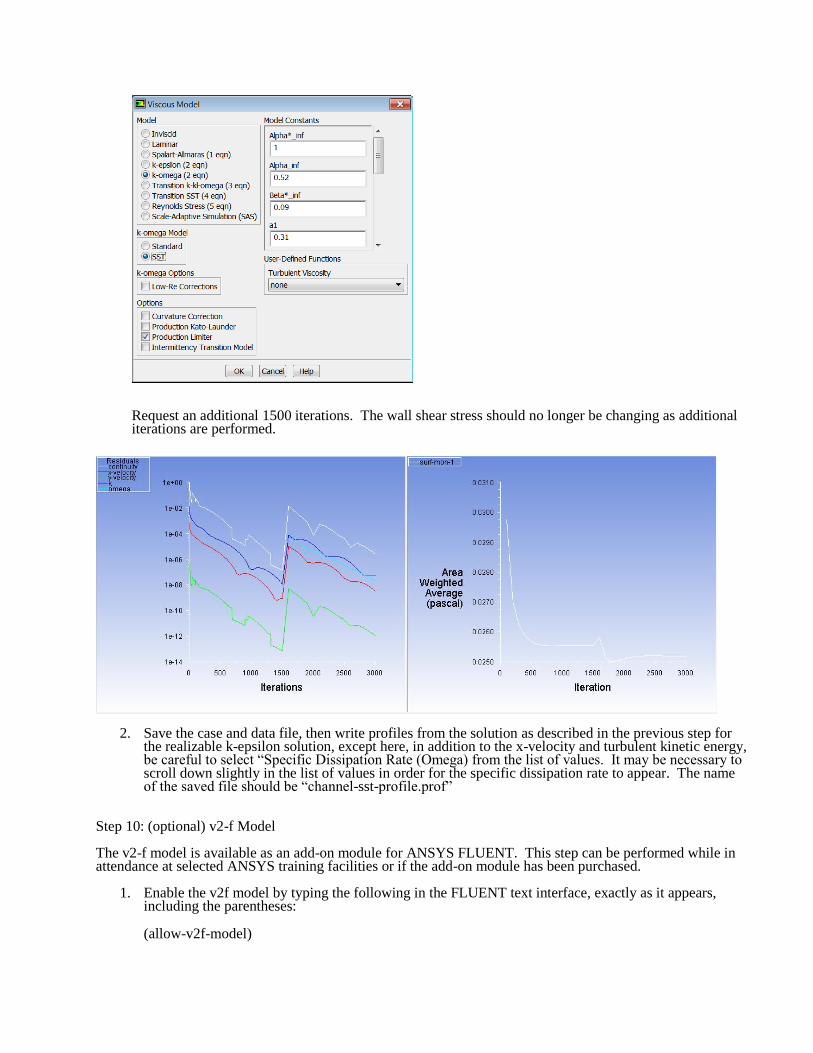
Request an additional 1500 iterations. The wall shear stress should no longer be changing as additional iterations are performed.

2. Save the case and data file, then write profiles from the solution as described in the previous step for the realizable k-epsilon solution, except here, in addition to the x-velocity and turbulent kinetic energy, be careful to select “Specific Dissipation Rate (Omega) from the list of values. It may be necessary to scroll down slightly in the list of values in order for the specific dissipation rate to appear. The name of the saved file should be “channel-sst-profile.prof”

Step 10: (optional) v2-f Model The v2-f model is available as an add-on module for ANSYS FLUENT. This step can be performed while in attendance at selected ANSYS training facilities or if the add-on module has been purchased.

1. Enable the v2f model by typing the following in the FLUENT text interface, exactly as it appears, including the parentheses:

(allow-v2f-model)

2. Open the Viscous Models panel and select the v2f model.

3. In Solution Methods, ensure that the spatial discretization for the “Velocity Variance Scale” and “Elliptic Relaxation Function” equations is set to Second Order Upwind. It may be necessary to use the scroll bar in the panel in order to be able to see all the equations in the list.

4. Perform an additional 2500 iterations. The solution monitors should appear as below:

5. Write profiles in the same way as you did for the SST and realizable k-epsilon models. The variables that need to be selected for the v2-f model are X Velocity, Turbulent Kinetic Energy, Turbulent Dissipation Rate, Velocity Variance Scale (v2) and Elliptic Relaxation Function. Name the file “channel-v2f-profile.prof”

6. Exit Fluent

Part 2. Calculating Flow in the Planar Diffuser Step 1. Mesh

1. Start FLUENT 2ddp. If multiple cores are available, there is a noticeable decrease in solution time using parallel FLUENT for 2 cores even though this is a very small mesh. Read “asymmetric-scaled.msh” and perform a mesh check. Although some warning messages were displayed upon reading the mesh, the mesh check reports no errors so it is safe to proceed.

Step 2. Models

1. Activate the realizable k-epsilon turbulence model with Enhanced Wall Treatment, as shown in Part 1 of this tutorial

Step 3. Materials

1. The fluid is standard air with constant density, so there is no need to visit the materials panel.

Step 4. Boundary Conditions

1. Go to Define > Boundary Conditions, or click on Boundary Conditions in the navigation pane on the left of the GUI. Below the boundary conditions panel is a button labeled “Profiles….”. Click this button, then click “Read…” on the Profiles panel and select the file “channel-rke-profile.prof” created in Part 1 of this tutorial. The panel will be populated as shown in the figure below. Click Close to close the panel.

2. Apply boundary conditions for inlet_v as shown in the figure below

3. Apply boundary conditions for “outlet” as shown in the figure below

Step 5: Solution Settings

1. Select Solution Methods in the navigation pane on the left of the GUI. Change the pressure-velocity coupling scheme to Coupled, set the spatial discretization schemes as shown in the figure below, and also select both “Pseudo Transient” and “High Order Term Relaxation” in the lower part of the panel.

2. Solution Controls: keep all the default settings in the Solution Controls panel 3. Initialize the Solution

a. Click Solution Initialization in the navigation pane on the left of the GUI. Below “Hybrid

Initialization” click “More Settings”, then click the “Turbulence Settings” tab, unselect “Averaged Turbulent Parameters” and enter the values shown in the panel, which are approximately the same as the average values computed in Part 1 for the channel upstream of the diffuser section.

b. Click “Initialize” to initialize the flow

4. Click Monitors in the navigation pane on the left of the GUI.

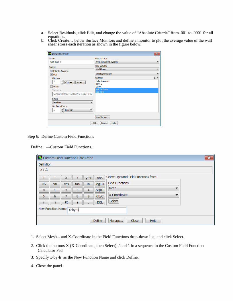
a. Select Residuals, click Edit, and change the value of “Absolute Criteria” from .001 to .0001 for all

equations. b. Click Create… below Surface Monitors and define a monitor to plot the average value of the wall

shear stress each iteration as shown in the figure below.

Step 6: Define Custom Field Functions

Define −→Custom Field Functions...

1. Select Mesh... and X-Coordinate in the Field Functions drop-down list, and click Select.

2. Click the buttons X (X-Coordinate, then Select), / and 1 in a sequence in the Custom Field Function

Calculator Pad

3. Specify x-by-h as the New Function Name and click Define.

4. Close the panel.

Step 7: Iterations and Convergence

1. Select Run Calculation in the navigation pane at the left of the GUI. Keep all of the default

settings in the Pseudo Transient Options section of the panel. Start the calculations by

requesting 10 iterations.

2. Use the TUI command /solve/monitor/surface/clear-data to reset the surface monitor data

3. Request another 300 iterations. The solution will reach the residual criteria at around 180 iterations. The

precise number of iterations may vary depending on your machine type.

4. Save the case and data files (asd-rke-diffuser-final).

5. Change the reference values

Report −→Reference Values...

(a) Change the Velocity value to 2.56. The bulk velocity for the channel flow at the diffuser

inlet should be used in order to ensure consistency with skin friction coefficient values

reported by (1).

(b) Change the Length value to 0.1.

6. Define a new custom field function as shown below. This will make the comparison of the skin friction

coefficient on the lower wall more convenient.

7. Plot the initial results

(a) Click Plots in the navigation pane on the left of the GUI and then XY plots in the center panel. Click

Set Up… to define the plot output.

(b) Deselect Node Values and Position on X Axis under Options.

(c) Select Custom Field Functions... and Skin Friction Coefficient under Y Axis Function.

(d) Select Custom Field Functions... and x-by-h under X Axis Function.

(e) Click Load File... and select the cf top.xy file and click OK.

in

Experimental data for skin friction coefficient (Cf = τw /0.5ρU 2 ) for the top wall and bottom

wall are stored in cf top.xy and cf bot.xy respectively.

(f) Change the line and symbol style for Curve 0.

i. Click on Curves... in the Solution XY Plot panel and enter values as shown below. Click Apply

and close the panel

ii. Make the changes as shown in the panel.

iii. Click Apply and close the panel.

(g) Select wall_top under Surfaces and click Plot.

(h) Repeat the same procedure for bottom wall by loading file cf bot and selecting

wall bottom under Surfaces.

Figure 2: Skin Friction Coefficient Vs x/h (RKE) for Top Wall

Figure 3: Skin Friction Coefficient Vs x/h RKE) for Bottom Wall

8. Save the case and data file one final time.

9. In the Viscous Model panel, select the SST k- model.

10. Select Boundary Conditions in the navigation pane on the left of the GUI. Click Profiles…, then

Delete, then Read and select “channel-sst-profile.prof”. Close the panel

11. Open the boundary conditions panel for inlet_v and select “periodic.1 specific-diss-rate” as the

boundary condition for the specific dissipation rate.

12. Click Solution Methods in the navigation pane on the left of the GUI. Change the spatial discretization

setting for turbulent kinetic energy and specific dissipation rate to “Second Order Upwind”. Keep all

the other settings.

13. Perform the iterations

a. Click Run Calculation in the navigation pane and request another 300 iterations. The solution

will converge at around 380 total iterations. Save the case and data file (asd-sst-diffuser-final)

before proceeding to the next step.

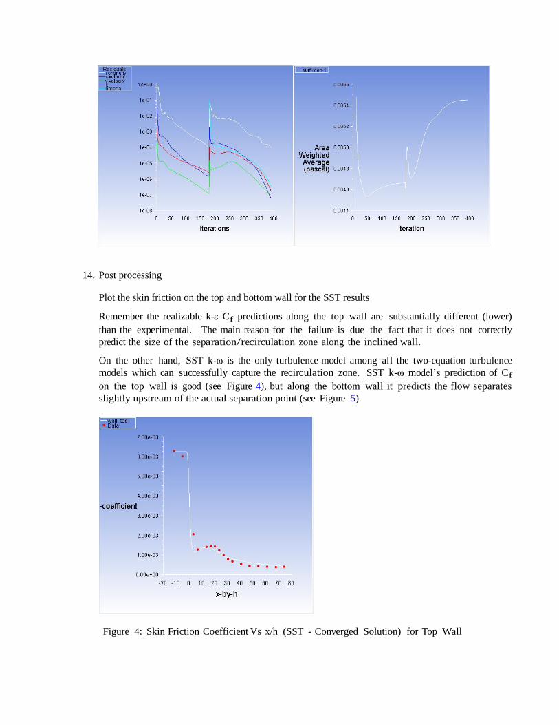
14. Post processing

Plot the skin friction on the top and bottom wall for the SST results

Remember the realizable k- Cf predictions along the top wall are substantially different (lower)

than the experimental. The main reason for the failure is due the fact that it does not correctly

predict the size of the separation/recirculation zone along the inclined wall.

On the other hand, SST k-ω is the only turbulence model among all the two-equation turbulence

models which can successfully capture the recirculation zone. SST k-ω model’s prediction of Cf

on the top wall is good (see Figure 4), but along the bottom wall it predicts the flow separates

slightly upstream of the actual separation point (see Figure 5).

Figure 4: Skin Friction Coefficient Vs x/h (SST - Converged Solution) for Top Wall

Figure 5: Skin Friction Coefficient Vs x/h (SST - Converged Solution) for Bottom Wall

Grid Independence Study

Test whether the converged results (from the SST k-ω model: asd-sst-diffuser-final.cas.gz, asd-sst-diffuser-

final.dat.gz) obtained so far are independent of the grid resolution, you can either uniformly double the

total cell count, or use the grid adaption feature of the solver to achieve the objective more efficiently.

Grid independence is attained when further mesh refinement yields only small and insignificant changes in

the solution fields. Different mesh adaption criteria could be considered, but here we choose to adapt a region

extending slightly upstream and slightly downstream of the separated flow region. If you proceed from your

own calculation, first save the case and data before attempting any adaption since any change is

irreversible. First, we will identify the separated flow region by creating an iso-surface where the x-velocity

is equal to zero.

1. Surface −→ Iso-Surface

Select Velocity, X-Velocity, click Compute, enter xvel=0 for the surface name and click Create

2. Show contours of X-Velocity, using the Draw Mesh option in the contour display panel to show the recirculation zone (xvel=0 surface).

3. Calculate the maximum x-coordinate of the iso-surface. There are other ways to identify the

downstream end of the recirculation zone, such as looking where the shear stress changes sign on the bottom wall, but the purpose here is simply to identify an appropriate region for grid adaption, so the most precise possible method is not required.

4. Open the Region Adaption panel.

Adapt −→ Region...

(a) Select the minimum and maximum coordinates as shown in the picture. The x-values

correspond to 0.15 m upstream of the diffuser section and downstream of the

recirculation zone.

(b) Click Mark, then Manage…, then Options…, then Draw Mesh and Filled, then click OK and

finally Display (in the Manage Adaption Registers panel). The region of cells to be adapted is

shown in the figure below. It is advisable to always visually confirm the location of the adaption

region.

(c) Click Adapt in the Manage Adaption Registers panel

(d) Save the case and data fi les (asd-ss t -diffuser -adapt -f inal)

(e ) In the Run Calculation panel, reduce the timescale factor from 1.0 to 0.5 and continue

iterating until the case is converged. Save the case and data files.

(f) Plot the results

Figure 6: Skin Friction Coefficient Vs x/h (sstkw) After Grid Adaption for Top Wall

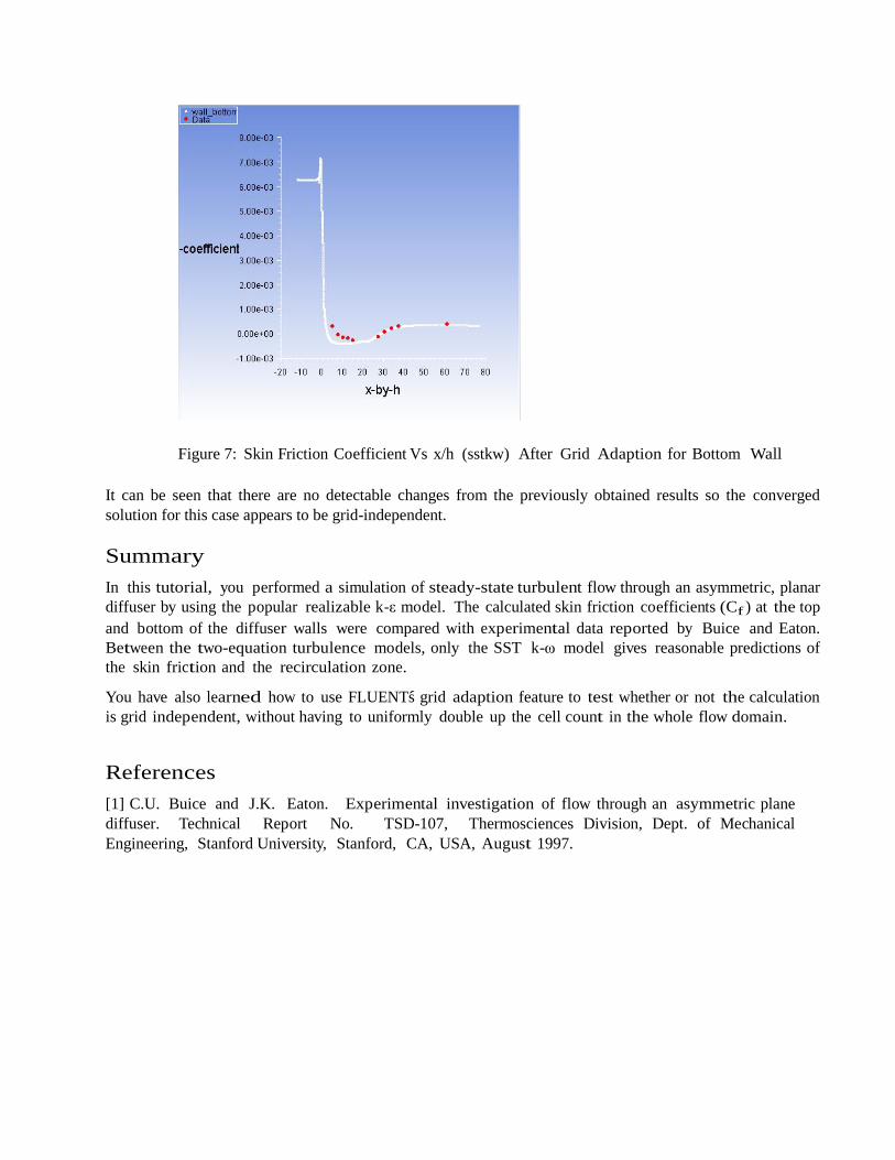
Figure 7: Skin Friction Coefficient Vs x/h (sstkw) After Grid Adaption for Bottom Wall

It can be seen that there are no detectable changes from the previously obtained results so the converged

solution for this case appears to be grid-independent.

Summary

In this tutorial, you performed a simulation of steady-state turbulent flow through an asymmetric, planar

diffuser by using the popular realizable k-ε model. The calculated skin friction coefficients (Cf ) at the top

and bottom of the diffuser walls were compared with experimental data reported by Buice and Eaton.

Between the two-equation turbulence models, only the SST k-ω model gives reasonable predictions of

the skin friction and the recirculation zone.

You have also learned how to use FLUENTs grid adaption feature to test whether or not the calculation

is grid independent, without having to uniformly double up the cell count in the whole flow domain.

References

[1] C.U. Buice and J.K. Eaton. Experimental investigation of flow through an asymmetric plane

diffuser. Technical Report No. TSD-107, Thermosciences Division, Dept. of Mechanical

Engineering, Stanford University, Stanford, CA, USA, August 1997.

(Optional) v2-f Calculation

The v2-f model is a little bit more difficult to converge in this case than the other turbulence models, so a

few additional steps are needed to set up the solution methods and controls

1. Read the case and data files from the RKE solution

2. In the TUI, type (allow-v2f-model) as described in Part 1, Step 10 of this tutorial and then

activate the v2f model in the Viscous Model panel

3. Select Boundary Conditions in the navigation pane on the left of the GUI and click Profiles.

Click Read and select channel-v2f-profile.prof

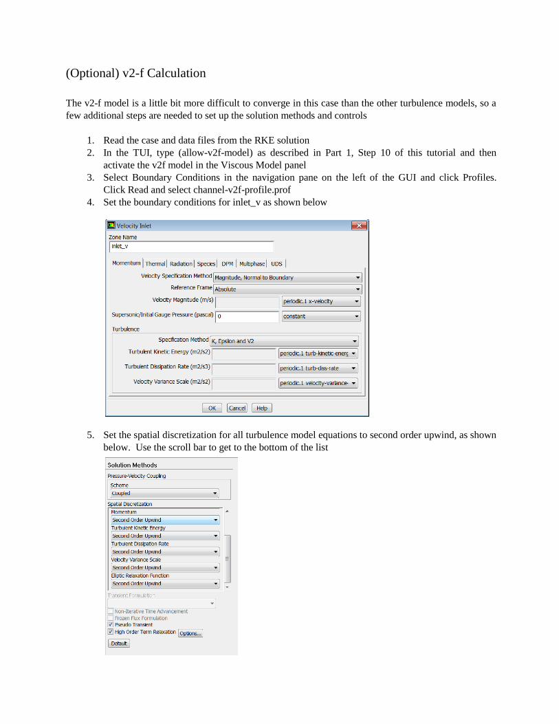
4. Set the boundary conditions for inlet_v as shown below

5. Set the spatial discretization for all turbulence model equations to second order upwind, as shown

below. Use the scroll bar to get to the bottom of the list

6. The RKE solution can be used as an initial condition for the v2-f calculation.

7. Request 250 iterations. The solution will converge smoothly.

8. Plot the skin friction coefficient for the top and bottom walls. The v2-f model accurately

captures the separation point and the size of the recirculation zone on the bottom wall.

Figure 8: Skin Friction Coefficient Vs x/h v2-f for Top Wall

Figure 9: Skin Friction Coefficient Vs x/h v2-f for Bottom Wall