Coot Tutorial

X-ray Methods, CSHL 2016

December 18, 2017

Contents

1 Mousing 3

2 Getting Started 32.1 Load tutorial data . . . . . . . . . . . . . . . . . . . . . . . . . . . 32.2 Adjust Virtual Trackball . . . . . . . . . . . . . . . . . . . . . . . 52.3 Display maps . . . . . . . . . . . . . . . . . . . . . . . . . . . . . 52.4 Zoom in and out . . . . . . . . . . . . . . . . . . . . . . . . . . . . 62.5 Recentre on Different Atoms . . . . . . . . . . . . . . . . . . . . . 62.6 Change the Clipping (Slab) . . . . . . . . . . . . . . . . . . . . . 82.7 Recontour the Map . . . . . . . . . . . . . . . . . . . . . . . . . . 92.8 Change the Map Colour . . . . . . . . . . . . . . . . . . . . . . . 92.9 Select a Map . . . . . . . . . . . . . . . . . . . . . . . . . . . . . . 9

3 Model Building 103.1 Rotamers . . . . . . . . . . . . . . . . . . . . . . . . . . . . . . . . 103.2 More Real Space Refinement . . . . . . . . . . . . . . . . . . . . . 11

4 Blobology 124.1 Find Blobs . . . . . . . . . . . . . . . . . . . . . . . . . . . . . . . 124.2 Blob 3 . . . . . . . . . . . . . . . . . . . . . . . . . . . . . . . . . . 134.3 Blob 2 . . . . . . . . . . . . . . . . . . . . . . . . . . . . . . . . . . 134.4 Blob 1 . . . . . . . . . . . . . . . . . . . . . . . . . . . . . . . . . . 14

5 Customise the Interface 15

6 Extra Fun (if you have time) 156.1 Waters . . . . . . . . . . . . . . . . . . . . . . . . . . . . . . . . . 156.2 Working with NCS . . . . . . . . . . . . . . . . . . . . . . . . . . 166.3 Add Terminal Residue . . . . . . . . . . . . . . . . . . . . . . . . 176.4 Display Symmetry Atoms . . . . . . . . . . . . . . . . . . . . . . 196.5 Skeletonization and Baton Building . . . . . . . . . . . . . . . . . 196.6 Refine with Refmac . . . . . . . . . . . . . . . . . . . . . . . . . . 19

1

7 Use the EDS and PDB REDO 207.1 Make a (Pretty?) Picture . . . . . . . . . . . . . . . . . . . . . . . 20

2

1 Mousing

First, how do we move around and select things?

Left-mouse Drag Rotate viewCtrl Left-Mouse Drag Translates viewShift Left-Mouse Label AtomRight-Mouse Drag Zoom in and outMiddle-mouse Centre on atomScroll-wheel Forward Increase map contour levelScroll-wheel Backward Decrease map contour level

2 Getting Started

In this tutorial, we will learn how to do the following:

1. Start Coot

2. Display coordinates

3. Display a map

4. Zoom in and out

5. Recentre on Different Atoms

6. Change the Clipping (Slab)

7. Recontour the Map

8. Change the Map Colour

9. Display rotamers and refine residue

2.1 Load tutorial data

To use coot, in a terminal window, type:$ cootWhen you first start coot, it should look something like Figure 1.So let’s read in the coordinates and data (and thus generate a map)To load the files on which we will be working:From Coot’s main menu bar, select Extensions → Load tutorial model and

data

3

Figure 1: Coot at StartupNot much to see at present... Actually, after this, coot screenshots will bedisplayed with a white background, whereas you will see a black one

Figure 2: Coot After Loading Coordinates

4

2.2 Adjust Virtual Trackball

By default, Coot has a “virtual trackball” to relate the motion of the moleculeto the motion of the mouse. Many people don’t like this.

So you might like to try the following. In the Coot main menu-bar:Edit → Preferences. . .[Coot displays a Preferences window]On the left toolbar select General and then on the right top notebook tab

HID. Select “Flat” to change the mouse motion.(Use the “Spherical Surface” option to turn it back to how it is by default).What is the difference? “Flat” mode is like the mode used by “O”. In both

modes, dragging the mouse near the centre of the screen causes the view torotate about the X- or Y- axis. However in spherical mode you can also rotateabout the z-axis by dragging the mouse along an edge of the window.

2.3 Display maps

We are at the stagewherewe are looking at the results of the refinement. The re-finement programs stores its data (labelled lists of structure factor amplitudesand phases) in an “MTZ” file. Let’s take a look. . .

Figure 3: Coot MTZ Column Label Selection Window

5

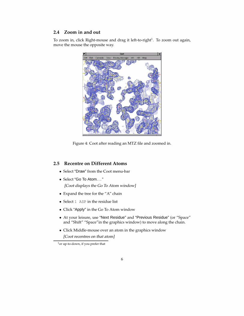
2.4 Zoom in and out

To zoom in, click Right-mouse and drag it left-to-right1. To zoom out again,move the mouse the opposite way.

Figure 4: Coot after reading an MTZ file and zoomed in.

2.5 Recentre on Different Atoms

• Select “Draw” from the Coot menu-bar

• Select “Go To Atom. . . ”

[Coot displays the Go To Atom window]

• Expand the tree for the “A” chain

• Select 1 ASP in the residue list

• Click “Apply” in the Go To Atom window

• At your leisure, use “Next Residue” and “Previous Residue” (or “Space”and “Shift” “Space”in the graphics window) to move along the chain.

• Click Middle-mouse over an atom in the graphics window

[Coot recentres on that atom]

1or up-to-down, if you prefer that

6

• Ctrl Left-mouse & Drag moves the view around. If this is a too slow andjerky:

– Select Edit → Preferences. . . from Coot’s menu-bar

– Select the “Maps” toolbutton on the left

– Select the “Dragged Map” notebook tab.

– Select “No” in the “Active Map on Dragging” window

– Click “OK” in the “Preferences” window

Now the map is recontoured at the end of the drag, not at each step2.

Another, additional way to make the movements faster is to change thenumber of steps for the “Smooth Recentering”. Again you find this in the“Preferences” (Preferences → General → Smooth Recentering). Changethe “Number of Steps” (the default is 40) to something smaller, e.g. 20.

Figure 5: Coot’s Go To Atom Window (it doesn’t look exactly like this anymore).

• You can display the contacts too, as you do this:

2which looks less good on faster computers.

7

– Select “Measures” from the Coot menu-bar

– Select “Environment Distances. . . ”

– Click on the “Show Residue Environment?” check-button

∗ Also Click “Label Atom?” if youwish the Cα atoms of the residuesto be labelled.

– Click “OK” in the Environment Distances window

– Click “Apply” in the Go To Atom window

[You can’t change the colour of the Environment distances]

Figure 6: Coot showing Atom Label and environment distances.

You can turn off the Environment distances if you like.

2.6 Change the Clipping (Slab)

• Select “Draw” from the Coot menu-bar

• Select “Clipping. . . ” from the sub-menu

[Coot displays a Clipping window]

• Adjust the slider to the clipping of your choice

• Click “OK” in the Clipping window

8

Alternatively, you can use “D” and “F”3 on the keyboard, or Control Right-mouse up/down (Control Right-mouse left/right does z-translation).

2.7 Recontour the Map

• Scroll your scroll-wheel forwards one click4

[Coot recontours the map using a 0.05electron/A3 higher contour level]

• Scroll your scroll-wheel forwards and backwards more notches and seethe contour level changing.

• If you don’t have a wheel on your mouse you can use “+” and “-” on thekeyboard.

• Note that the “Scroll” button in the Display Manager allows you to selectwhich map is affected by this5.

2.8 Change the Map Colour

• Select “Edit” from the Coot menu-bar

• Select “Map Colour” in the sub-menu

• Select “1 xxx FWT PHWT” in the sub-menu

[Coot displays a Map Colour Selection window]

• Choose a new colour by clicking on the colour widgets

[Coot changes the map colour to match the selection ]

• Click “OK” in the Map Colour Selection window

2.9 Select a Map

Select a map for model building. We prefer you to use the modelling toolbaricon buttons (here “Map”) displayed on the right side of the Coot window.Note: If you are not sure which icon corresponds to which function look at thedisplayed tips when over the button with the mouse. Or change the displaystyle of the buttons by clicking on the bottom arrow and select another style toget only or additionally text displayed.

Right Toolbar: “Map” from the Modelling Toolbar

click OK (you want to select the map with “. . . FWT PHWT”)

Alternatively you can use the Model/Fit/Refine window:

3think: Depth of Field.4don’t click it down.5by default it is the last map, which is not necessarily the map that you want.

9

Menubar: Calculate → Model/Fit/Refine...[Coot displays the Model/Fit/Refine window]

Select “Select Map. . . ” from the Model/Fit/Refine window

click OK (you want to select the map with “. . . FWT PHWT”)

Note: Most options found in the Model/Fit/Refine window are availablein the Modelling Toolbar too. You can change this with Preferences.

3 Model Building

“So what’s wrong with this structure?” you might ask.There are several ways to analyse structural problems and some of them

are available in Coot.

Validate → Density Fit Analysis → tutorial-modern.pdb[Coot displays a bar graph]

Look at the graph. The bigger and redder the bar the worse the geometry.There are 2 area of outstanding badness in the A chain, around 41A and 89A.

Let’s look at 89A first - click on the block for 89A.

[Coot moves the view so that 89A CA is at the centre of the screen ]

3.1 Rotamers

• Examine the situation. . . [ The sidechain is pointing the wrong way. Let’s Fixit...]

• Modelling Toolbar: Select the “Rotamers” button

• Alternatively:

Menubar: Calculate → Model/Fit/Refine...

[Coot displays the Model/Fit/Refine window]

Select “Rotamers” from the Model/Fit/Refine window.

• In the graphics window, (left-mouse) click on an atom of residue 89A (theCγ, say)

[Coot displays the “Select Rotamer” window]

• Choose the Rotamer that most closely puts the atoms into the side-chaindensity

• Click “Accept” in the “Select Rotamer” window

[Coot updates the coordinates to the selected rotamer]

10

• Click “Real Space Refine Zone” in the Model/Fit/Refine window6.

• In the graphics window, click on an atom of residue 89A. Click it again.

[Coot displays the refined coordinates in white in the graphics and a new“Accept Refinement” window]

• Click “Accept” in the “Accept Refinement” window.

[Coot updates the coordinates to the refined coordinates. 89A now fitsthe density nicely.]

OK. That’s good.Now, how about if we just use Real Space Refinement only?

• Click “Undo” twice

[Coot puts the sidechain back to the original position]

• Click “Real Space Refine Zone” in the Modelling Toolbar 7.

• In the graphics window, click on an atom of residue 89A. Click it again.

[Coot displays the refined coordinates in white in the graphics and a new“Accept Refinement” window]

• Now using left-mouse, click and drag on the intermediate (white) CZatom of the PHE (if you mis-click the atom, the view will rotate).

• Can you pull the atom around so that the side-chain fits the density?

[Yes, you can]

3.2 More Real Space Refinement

Now let’s have a look at the other region of outstanding badness:

• Click on the graph block for 41 A

[Coot moves the view so that 41A CA is at the centre of the screen]

• Examine the situation. . .

• Residue 41 is in a mess and not fitting to the density. Can you fix it?

[Yes, you can]

• The trick is Real Space Refine that zone. So. . .

• You can either Real Space Refine a few residues (40, 41 and 42) or just 41.Take your pick.

6. . . or use the modelling toolbar button7. . . or in the Model/Fit/Refine window

11

Figure 7: 89A now fits the density nicely.

• Click on “Real Space Refine Zone” in theModelling Toolbar (Model/Fit/Refinewindow)

• Select a range by clicking on atoms in the graphics window (either atomsin 40 then 42 or an atom in 41 twice)

[Coot displays intermediate (white) atoms]

• Click and drag on some atoms until the atoms fit nicely in the density.

If you want to move a single atom then Ctrl Left-mouse to pick and move(just) that intermediate atom.

[Note: Selecting and moving just the Carbonyl Oxygen is a good idea - use CtrlLeft-mouse to move just one atom.]

4 Blobology

4.1 Find Blobs

To be found under Validate (called “Unmodelled Blobs”).You can use the defaults in the subsequent pop-up. Press “Find Blobs” and

wait a short while.You will get a newwindow that tell you that it has found unexplaned blobs.

Time to find out what they are.

12

4.2 Blob 3

Let’s start from Blob 3 (the blobs are ordered biggest to smallest - Blobs 3 and4 (if you have it) are the smallest).

• Click on “Blob 3”

[Coot centres the screen on a blob]

• Examine the situation. . .

[We need something tetrahedral there. . . ]

• “Place Atom At Pointer” on the Modelling Toolbar 8

[Coot shows a Pointer Atom Type window]

• “SO4” in the new window. . .

• In the “Pointer AtomAdded toMolecule:” frame, change “NewMolecule”to ‘‘tutorial-modern.pdb”

• Click OK.

• Examine the situation. . .

• the orientation is not quite right.

• Let’s Real Space Refine it (you should know what to do by now. . . )

• (“Real Space Refine Zone” then click an atom in the SO4 twice. Accept)

[The SO4 fits better now].

Blob 4 is like Blob 3 (isn’t it?)

4.3 Blob 2

Click on the button “Blob 2” and examine the density. Something is missingfrom the model. What?

This protein and has been co-crystallizedwith its ligand substrate, 3’ guano-sine monophosphate.

How do we add that?

• File → Seach Monomer library. . .

• Type guanosine in the box.

• Find the box for 3GP and press return. . .

[3GP appears]

It is often easier to work without hydrogens, so let’s delete them for now

8also available in Model/Fit/Refine window

13

• “Delete. . . ” from the Modelling Toolbar 9

• “Hydrogens in Residue”

• click on an atom in 3GP

[Hydrogens disappear]

The 3GP is displaced from where we want it to be.

• Calculate → Other Modelling Tools → Find Ligands. . .

• In the “Select Ligands” fram, click on the checkbutton for the ’3GP’ ligand

• Double-check the protein model and the map are the ones that you wantthem to be (the defaults should be fine).

• Click Find Ligands

You can adjust the position of the atoms of the ligand using Real SpaceRefinement

• Click on an atom in the ligand

[Coot adds intermediate white atoms and Refinement dialog ]

• Now pull on the atoms until you are satisfied then press OK

If you like the solution, you can merge this ligand into the protein:

• Calculate → Merge Molecules. . .

• Click (activate) “monomer-3GP.pdb”

• into Molecule:

tutorial-modern.pdb

• Merge

4.4 Blob 1

• Click on “Blob 1”

• Examine the situation. . .What is this density?

[We need to add residues to the C-terminus of the A chain.]

The missing residues are GLN, THR, CYS (QTC).

• Calculate → Fit Loop. . . Fit Loop by Rama Search. . .

[Coot pops-ups a Fit Loop dialog]

Add residue number 94 to 96 in the A chain.

The single letter codes of the extra residues are QTC

9Found in the Model/Fit/Refine window too

14

• Make sure that you can see the unmodelled density well, then click “FitLoop”

• Watch. . . (fun eh?)

• Examine the density fit.

[It should be fine, except at the C-terminus. We need to add an OXTatom to the residue]

• Calculate → Other Modelling Tools. . .

• Add OXT to Residue. . .

• Add it

——————————————————This is a far as I expect you to get.

——————————————————

5 Customise the Interface

You can add extra buttons to the interface:

• Move the curor to the right of the vertical separator in the horizontal toolbar (to the right of the icon for the ligand)

• Right Mouse click

• Click on the check-buttons for the extra tools you want to add

[Coot adds new Buttons for the selected functions in the horizontal tool-bar]

• Click Apply

• Click on Manage Buttons (add, delete buttons)

6 Extra Fun (if you have time)

6.1 Waters

Fit waters to the structure

• “Find Waters. . . ” in the Other Modelling Tools dialog 10, then OK (usingthe defaults)

[Waters appear]

10In older versions of Coot, the FindWaters button can be found in theModel/Fit/Refine dialogor the water drop in the modelling toolbar

15

To check the waters:

• Click on “Measures” in the main menubar.

• Click on Environment Distances

• Click on the “Show Residue Environment?” check-button

• Change the distances as you like

• Use the Go To Atomwidget to go to the first water (probably towards theend of the list of residues in Chain “W”)

• Use the Spacebar to navigate to the next residue (and Shift Spacebar togo backwards)

• If you don’t like the fast sliding11 you can turn it off (if you haven’t doneso already):

– Click Edit → Preferences. . . in the main menubar

– Click General → “Smooth Recentering...”

– Click “No”

6.2 Working with NCS

The tutorial data has two-fold NCS. With good data it is interesting to investi-gate the differences between the NCS copies. This may be done by comparingthe NCS related electron density, comparing the NCS related chains, or com-paring the Ramachandran plots for related chains:

• Comparing the NCS related electron density.

Go to Calculate/NCS maps and select the first map and model. Now,if you go to anywhere in the A chain, you will see two sets of electrondensity - the original density for the A chain, and the density for the Bchain transformed to overlap the A chain density. This gives you a visualcomparison of any differences.

Look at the density in the B molecule. Why does the density not agreehere? (Hint: the NCS is not a 2-fold rotation in this case, it is improper).

• Comparing the NCS-related chains.

Go to Draw/NCS ghost control and select Display non-crystallographicghosts. You will now see a copy of the B chain superimposed on theA chain. The B chain is draw using thin bonds.

Look for regions where the models differ. Using the NCS maps tool,check that the differences in the models are supported by the density.

11it’s not very good for water checking

16

• Compare the NCS-related chains using “NCS jumping”.

This is an alternative way of examining NCS similarities and differences.Use the Display Manager to undisplay the NCS maps you recently cre-ated above.

Use the “Goto Atom” dialog and press the “Update from Current Posi-tion” button.

[Coot shifts the centre of the screen to the closest displayed CA atom]

Identify the chain that you are looking at (for example, by double-clickingon an atom)

Now press the “o” key on the keyboard.

[Coot shifts the centre of the screen to a NCS-related chain]

Identify the chain that you are looking at now.

Press “o” again.

What is happening?

(Note: ”o” stands for “Other NCS-related chain”.)

• Comparing the Ramachandran plots for related chains.

Go to Validate/Kleywegt plot. Check the Use specific chain options andselect chains A and B. You will get a Ramachandran plot with equivalentresidues from the A and B chains linked by arrows. Long arrows indicatesignificant differences. Click on a dot to view the residue concerned.

Another tool for identifying NCS differences is the Validate/NCS differ-ences graph. This gives a clickable histogram of differences.

6.3 Add Terminal Residue

[To be found on the Modelling Toolbar12]

• Use the Go To Atom window to go to residue 72 A.

• What do you see?

[You see missing atoms (that is, you don’t see them). This residue is supposed tobe a CYS! Bad things have happened to it. Let’s get rid of this residue. ]

[There may also be waters in the side-chain positions too (they have to be removedtoo).]

• Delete. . .

• (Make sure “Residue/Monomer” is active)

12and in the Model/Fit/Refine window

17

• Click on an atom of residue 72 A.

[Residue 72 A disappears]

• Lets’ put back an ALA.

• Add Terminal Residue. . .

[Coot adds intermediate white atoms and pops up a dialog]

• Accept the new atoms

OK, we now have a ALA. We want a CYS:

• Mutate & Auto Fit. . .

• Click on an atom in the new ALA

[Coot pops up a residue type chooser]

• Choose residue type CYS

[Coot mutates and fits a CYS]

• Examine the situation.

[ There is an extra blob of density on that CYS. What is it?] It is an alternativeconformation.

Let’s model it

• Add Alt Conf. . .

[Coot pops up a residue splitter dialog]

• Choose how you want to split your residue (the Right Way is an unre-solved philosophical issue. . . 13)

• Click on an atom in 72 A

[Coot adds intermediate white atoms and pops up a Rotamer Chooser]

• Choose the correct rotamer - it shouldn’t be difficult to tell which is theclosest.

• Accept when you are happy with you choice.

• Now optimize the fit of this new residue with Real Space Refinement.

The refinement of each alternate conformations is independent.

• Real Space Refine Zone

• click on (say) SG,B of 72A

• Press “A” (on the keyboard)

[Coot moves the atoms a bit]

13Actually Jane Richardson may disagree with that statement.

18

• Accept

• Now do the same with the other conformation.

[Ahhh! Much better.]

6.4 Display Symmetry Atoms

To be found on “Draw” → “Cell & Symmetry” menu item in the main menu.Try:

• Show Symmetry Atoms? → Yes

• Symmetry as Calphas? [on]

• Colour symmetry by molecule [on]

• Symmetry Radius 30A

• Colour Merge → 0.1

• Show Unit Cell? [on]

• OK

• Zoom out and have a look at how the molecules pack together.

6.5 Skeletonization and Baton Building

You can calculate the map skeleton in Coot directly:Calculate → Map Skeleton... → On.This can be used to “baton build” a map. You can turn off the coordinates

and try it if you like (the Baton Building window can be found by clicking “CaBaton Mode. . . ” in the Other Modelling Tools dialog14).

If you want to do this, I suggest you use Go To Atom and start residue 2 A(this allows you to build the complete A chain in the correct direction (it takesabout 15minutes or so) and you can compare it to the real structure afterwards.

Remember, when you start, you are placing a CA at the baton tip and atthe start you are placing atom CA 1. This might seem that you are “double-backing” on yourself - which can be confusing the first time.

6.6 Refine with Refmac

Refmac is a program that does Maximum Likelihood refinement of the model,and the interface to it can be found on the Model/Fit/Refine dialog. (By de-fault there is no icon on the toolbar for this action - open the window from

14this is quite advanced

19

the calculate menu15). Now click on “Run Refmac. . . ” (at the bottom of theModel/Fit/Refine window).

The defaults should be fine...“Run Refmac” in the new window. . .. . .Wait. . .[The cycle continues. . . ]

• Use “Validate → Difference Map Peaks” to find interesting features in thenewly created map and model.

• Python enabled version only: a dialog with geometric outliers and otherinteresting things (if they exist) detected by Refmac shows up 16.

7 Use the EDS and PDB REDO

• Let’s validate a structure deposited in the PDB.

• Use a web browser and go to http://eds.bmc.uu.se/eds/. Use thekeyword search to find the structure of a particular protein/ligand/author.

• File → Fetch PDB & Map Using EDS. . .

• Get the accession code and paste it into the entry box that pops up.

• Similarly, we can retrieve files from the PDB REDO server - this actuallyrefines the deposited structure against the deposited data, which oftenresults in a better map and model.

• Use the validation tools in Coot to examine how good a PDB file this is...

• [the Difference Map Peaks can be interesting]

7.1 Make a (Pretty?) Picture

(Depends on the appropriate supporting software17 being available):

• Arrange a nice view

• Press F8

• Wait a few seconds. . .15or add your own “Run Refmac” button to the toolbar or the main/top toolbar. To add the

button to the modelling/side toolbar, open the “Preference” window. Now go to Preferences →

General → Refinement Toolbar. In the right hand window scroll down and tick the box besides“Run Refmac. . . ”. A corresponding button will appear on the modelling toolbar. Alternativelyyou can add your own “Run Refmac. . . ” button to the top toolbar of the Coot window (only inPython versions). Click Right-mouse on the toolbar (besides the “Display Manager” button) andyou will see a pop-up menu. Select “Manage Buttons”, tick the box besides “Add Alt Conf” andclick “Apply”. A new button named “Add Alt Conf” will appear on the toolbar.

16This is an analysis from the Refmac log file and can alternatively be opened from Extensions...→ Refine... → Read REFMAC log

17Ethan Merritt’s Raster3D

20

Colophon

This document is written using XEmacs 21.5 in LATEX using AUCTEX and isdistributed with the Coot source code.

21