tutorial for new mosflm gui - bgulifeserv.bgu.ac.il/wb/zarivach/media/documentation/imosflm... ·...

MOSFLM tutorial for the new Interface

1. Introduction

1.1 Background

MOSFLM can process diffraction images from a wide range of detectors and produces, as output, an MTZ fileof reflection indices with their intensities and standard deviations (and other parameters). This MTZ file ispassed onto other programs of the CCP4 program suite (POINTLESS, SORTMTZ, SCALA, TRUNCATE)for further data reduction.

The MOSFLM program was originally written to process data collected on film. It was then modified toprocess data collected using the image plate detector developed at the EMBL outstation in Hamburg by JulesHendrix and Arno Lentfer, and the name was changed to ipmosflm. This is the current version of the program,which will also process data from CCD and pixel detectors.

1.2 Installation

The new GUI (imosflm) is currently available for Windows, Mac OSX and Linux platforms. A For details ofinstallation visit http://www.mrc-lmb.cam.ac.uk/harry/mosflm and follow the link to the New GUI imosflm.

1.3 Documentation

There are two distinct sources of documentation for MOSFLM, although neither of these currently makes anyreference to the new GUI. At present, this document is the only documentation available for the new GUI.

The MOSFLM user guide. This is available as a plain text file (mosflm_user_guide.txt) or on the web(www.mrc-lmb.cam.ac.uk/harry/mosflm/) as a PDF or HTML document. It is a very good idea tolook through this guide before starting serious data processing with MOSFLM, although you do notneed it for this tutorial.

1.

The "on-line" help. If you type "help" at the "MOSFLM =>" prompt (after starting the program) allpossible keywords are listed, with information on each keyword. This information is stored in an asciifile (mosflm.hlp) which can also be read (and searched) with an editor. This relies on having theenvironment variable "CCP4_HELPDIR" set to the directory containing this file. This is alsoavailable on the MOSFLM web pages under "keyword synopses"

2.

1.4 Aims of the tutorial

Your task is to process 84 images, hg_001.mar1600 to hg_084.mar1600, collected on a Mar345 image platedetector at a synchrotron beamline. These are crystals of a small domain (91 aa) that have been soaked in amercury compound, resulting in a dataset with a strong anomalous signal which can easily be used to solvethe structure. These images have kindly been provided by Camillo Rosano.

Tutorial for New Mosflm GUI

MOSFLM tutorial for the new Interface 1

http://www.mrc-lmb.cam.ac.uk/harry/mosflm

2. Overview of the new GUI

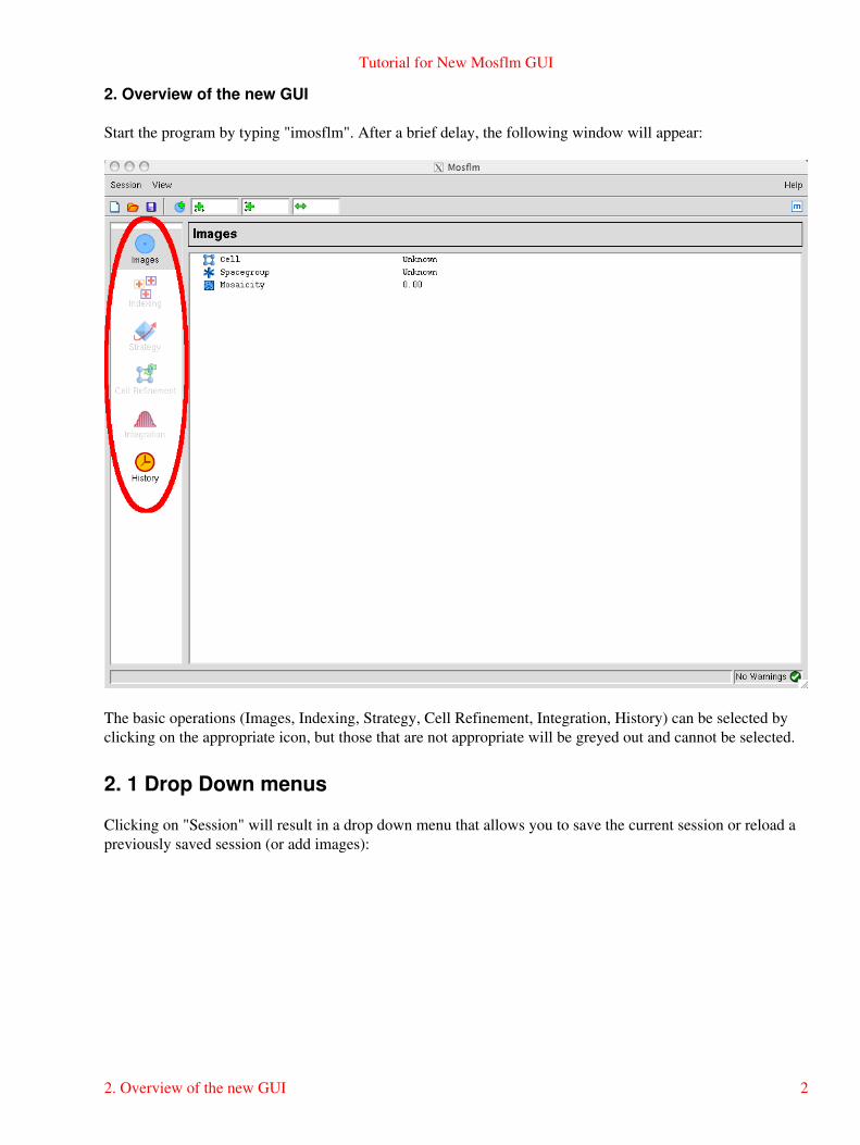
Start the program by typing "imosflm". After a brief delay, the following window will appear:

The basic operations (Images, Indexing, Strategy, Cell Refinement, Integration, History) can be selected byclicking on the appropriate icon, but those that are not appropriate will be greyed out and cannot be selected.

2. 1 Drop Down menus

Clicking on "Session" will result in a drop down menu that allows you to save the current session or reload apreviously saved session (or add images):


2. Overview of the new GUI 2

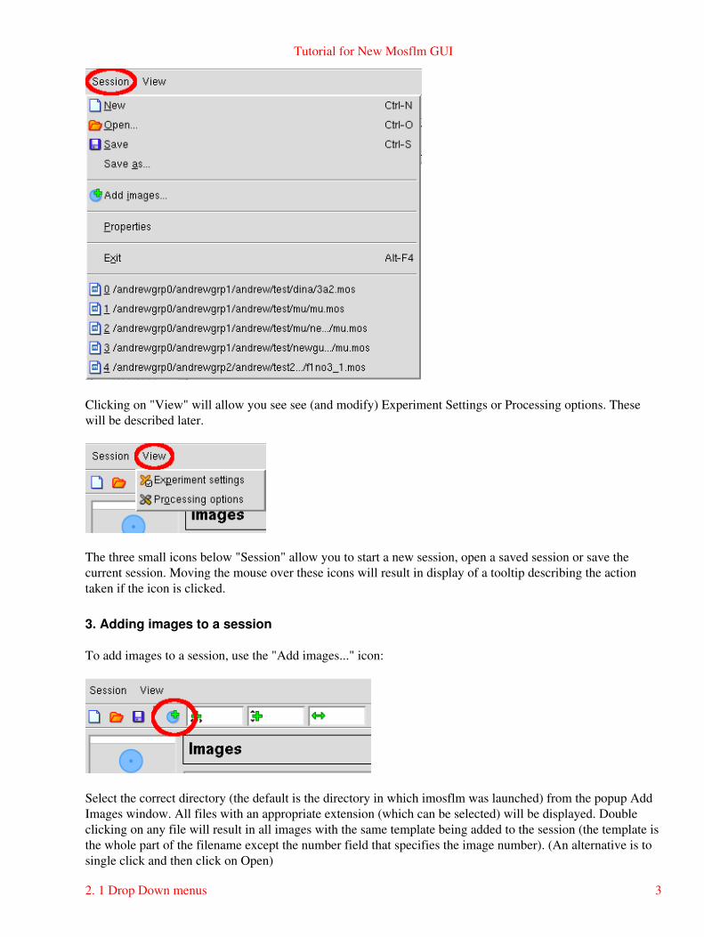
Clicking on "View" will allow you see see (and modify) Experiment Settings or Processing options. Thesewill be described later.

The three small icons below "Session" allow you to start a new session, open a saved session or save thecurrent session. Moving the mouse over these icons will result in display of a tooltip describing the actiontaken if the icon is clicked.

3. Adding images to a session

To add images to a session, use the "Add images..." icon:

Select the correct directory (the default is the directory in which imosflm was launched) from the popup AddImages window. All files with an appropriate extension (which can be selected) will be displayed. Doubleclicking on any file will result in all images with the same template being added to the session (the template isthe whole part of the filename except the number field that specifies the image number). (An alternative is tosingle click and then click on Open)


2. 1 Drop Down menus 3

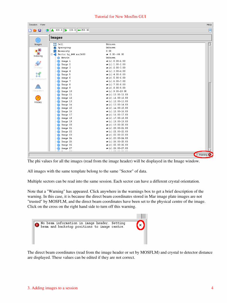
The phi values for all the images (read from the image header) will be displayed in the Image window.

All images with the same template belong to the same "Sector" of data.

Multiple sectors can be read into the same session. Each sector can have a different crystal orientation.

Note that a "Warning" has appeared. Click anywhere in the warnings box to get a brief description of thewarning. In this case, it is because the direct beam coordinates stored in Mar image plate images are not"trusted" by MOSFLM, and the direct beam coordinates have been set to the physical centre of the image.Click on the cross on the right hand side to turn off this warning.

The direct beam coordinates (read from the image header or set by MOSFLM) and crystal to detector distanceare displayed. These values can be edited if they are not correct.


3. Adding images to a session 4

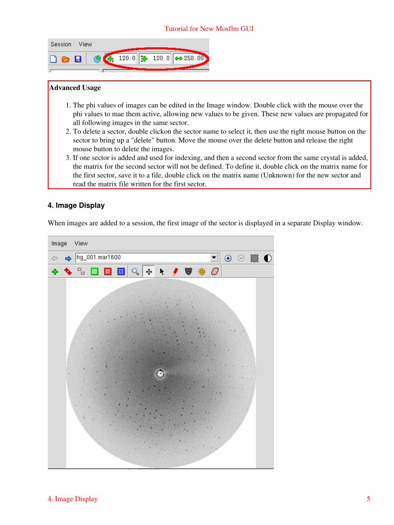
Advanced Usage

The phi values of images can be edited in the Image window. Double click with the mouse over thephi values to mae them active, allowing new values to be given. These new values are propagated forall following images in the same sector.

1.

To delete a sector, double clickon the sector name to select it, then use the right mouse button on thesector to bring up a "delete" button. Move the mouse over the delete button and release the rightmouse button to delete the images.

2.

If one sector is added and used for indexing, and then a second sector from the same crystal is added,the matrix for the second sector will not be defined. To define it, double click on the matrix name forthe first sector, save it to a file, double click on the matrix name (Unknown) for the new sector andread the matrix file written for the first sector.

3.

4. Image Display

When images are added to a session, the first image of the sector is displayed in a separate Display window.


4. Image Display 5

The "Image" drop down menu allows display of the previous or next image in the series. The "View" dropdown menu allows the image to be displayed in different sizes (related by scale factors of two), based on theimage size and the resolution of the monitor.

The line below allows selection of different images, either using right and left arrow or selecting one from thedrop down list of all images in that sector. (The image being displayed can also be changed bydouble-clicking on an image name in the main "Images" window.)

"+" and "-" will zoom the image without changing the centre. The "Fit image" icon will restore the image toits original size (right mouse button will have the same effect). The "Contrast" icon will give a histogram ofpixel values. Use the mouse to drag the vertical dotted line, to the right to lighten the image, to the left todarken it. Try adjusting the contrast.

4.1 Display Icons

The six icons on the left, control the display of the direct beam position, spots found for indexing, predictedspots, masked areas, spot-finding search area and resolution limits respectively.

These are followed by icons for Zoom, Pan and Selection Tools, and tools for adding spots manually (forindexing), editing masks, circle fitting and erasing spots or masks.

4.1.1 Masked areas .... circular beamstop shadow

Select the masked area icon. A green circle will be display showing the default position and size of thebackstop shadow.

Make sure that the Zoom icon (magnifying glass) is selected and use the left-mouse-button (abbreviated toLMB in following text) to drag out a rectangle around the centre of the image. The inner dotted yellowrectangle will show the part of the image that will actually appear in the zoom.


4.1 Display Icons 6

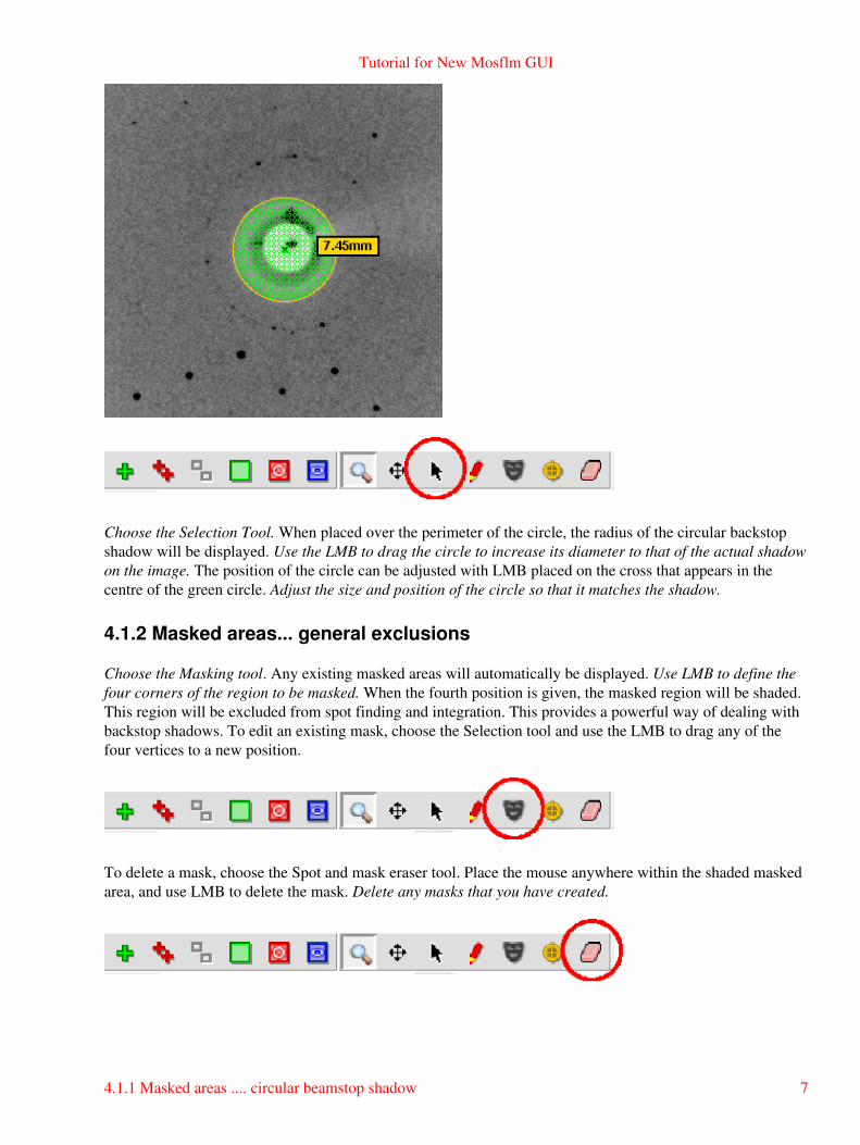
Choose the Selection Tool. When placed over the perimeter of the circle, the radius of the circular backstopshadow will be displayed. Use the LMB to drag the circle to increase its diameter to that of the actual shadowon the image. The position of the circle can be adjusted with LMB placed on the cross that appears in thecentre of the green circle. Adjust the size and position of the circle so that it matches the shadow.

4.1.2 Masked areas... general exclusions

Choose the Masking tool. Any existing masked areas will automatically be displayed. Use LMB to define thefour corners of the region to be masked. When the fourth position is given, the masked region will be shaded.This region will be excluded from spot finding and integration. This provides a powerful way of dealing withbackstop shadows. To edit an existing mask, choose the Selection tool and use the LMB to drag any of thefour vertices to a new position.

To delete a mask, choose the Spot and mask eraser tool. Place the mouse anywhere within the shaded maskedarea, and use LMB to delete the mask. Delete any masks that you have created.


4.1.1 Masked areas .... circular beamstop shadow 7

4.1.3 Spot search area Select the Show spotfinding search area icon. The inner andouter radii for the spot search will be displayed as shown below. If theimages are very weak, the spot finding radius will automatically be reduced,but this provides additional control.

Either can be changed by dragging with the LMB. Do not change the radii for these images.

Advanced Usage

The red rectangle displays the area used to determine an initial estimate of the background of the image . It isimportant that this does not overlap significant shadows on the image. It can be shifted laterally or changedin orientation (in 90° steps) by dragging with the LMB.

4.1.4 Resolution limits

Select the Show resolution limits icon. The low and high resolution limits will be displayed. The resolutionlimits can be changed by dragging the perimeter of the circle with LMB (make sure that the Selection Toolhas been chosen). The resolution limits will affect Strategy, Cell refinement and Integration, but not spotfinding or indexing. The low resolution is not strictly correct (it falls within the backstop shadow) but does notneed to be changed because spots within the backstop shadow will be rejected.


4.1.3 Spot search area Select the Show spotfinding search area icon. The inner and outer radii for the spot search will be displayed as shown below. If the images are very weak, the spot finding radius will automatically be reduced, but this provides additional control.8

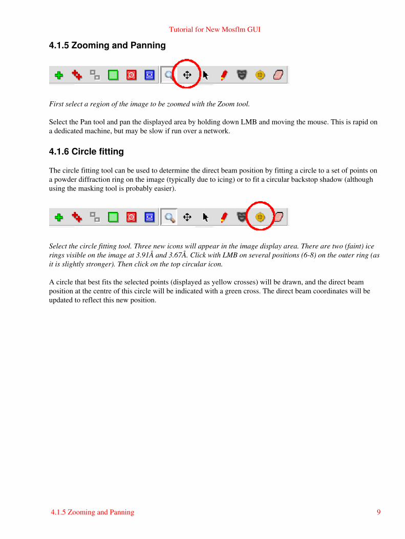
4.1.5 Zooming and Panning

First select a region of the image to be zoomed with the Zoom tool.

Select the Pan tool and pan the displayed area by holding down LMB and moving the mouse. This is rapid ona dedicated machine, but may be slow if run over a network.

4.1.6 Circle fitting

The circle fitting tool can be used to determine the direct beam position by fitting a circle to a set of points ona powder diffraction ring on the image (typically due to icing) or to fit a circular backstop shadow (althoughusing the masking tool is probably easier).

Select the circle fitting tool. Three new icons will appear in the image display area. There are two (faint) icerings visible on the image at 3.91Å and 3.67Å. Click with LMB on several positions (6-8) on the outer ring (asit is slightly stronger). Then click on the top circular icon.

A circle that best fits the selected points (displayed as yellow crosses) will be drawn, and the direct beamposition at the centre of this circle will be indicated with a green cross. The direct beam coordinates will beupdated to reflect this new position.


4.1.5 Zooming and Panning 9

4.2 Other functionalities

Right mouse button will return the display to the full size image, if it is zoomed.

To get a small zoom window that can be moved over the image, hold down "Shift" with the Zoom toolselected. The area within the dotted square will be zoomed within the solid square.

Holding down "Alt" (or "Command" ⌘ on Macs) will display the resolution at the current mouse position. Ifpositioned over a found spot, the spot coordinates and I/σ(I) will be given.

If positioned over a predicted spot, the indices of that spot will be given.

5. Spot finding, indexing and mosaicity estimation

When images have been added, the "Indexing" operation becomes accessible (it is no longer greyed out).

Click on Indexing. This will bring up the major Indexing window in place of the Images window.

5.1 Spot Finding

By default, two images 90 apart in phi (or as close to 90 as possible) will be selected and a spot search carriedout on both images.

Found spots will be displayed as crosses (red for those above the intensity threshold, yellow for those below).They will also be shown in the Image Display window.


4.1.6 Circle fitting 10

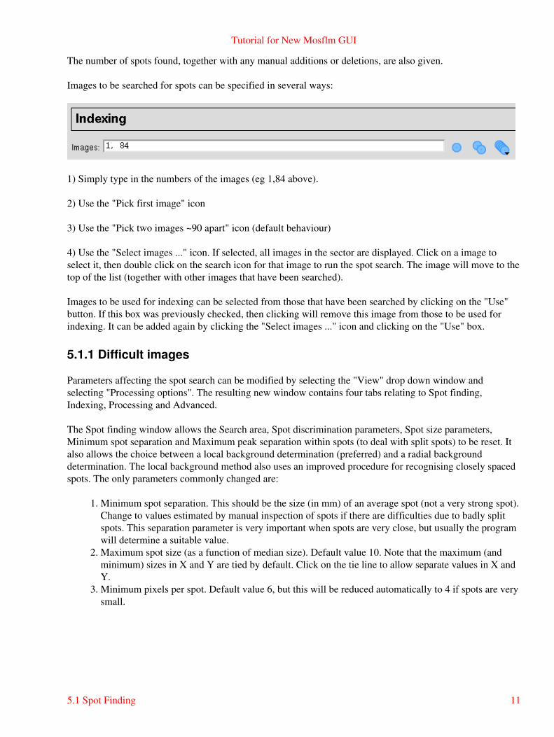
The number of spots found, together with any manual additions or deletions, are also given.

Images to be searched for spots can be specified in several ways:

1) Simply type in the numbers of the images (eg 1,84 above).

2) Use the "Pick first image" icon

3) Use the "Pick two images ~90 apart" icon (default behaviour)

4) Use the "Select images ..." icon. If selected, all images in the sector are displayed. Click on a image toselect it, then double click on the search icon for that image to run the spot search. The image will move to thetop of the list (together with other images that have been searched).

Images to be used for indexing can be selected from those that have been searched by clicking on the "Use"button. If this box was previously checked, then clicking will remove this image from those to be used forindexing. It can be added again by clicking the "Select images ..." icon and clicking on the "Use" box.

5.1.1 Difficult images

Parameters affecting the spot search can be modified by selecting the "View" drop down window andselecting "Processing options". The resulting new window contains four tabs relating to Spot finding,Indexing, Processing and Advanced.

The Spot finding window allows the Search area, Spot discrimination parameters, Spot size parameters,Minimum spot separation and Maximum peak separation within spots (to deal with split spots) to be reset. Italso allows the choice between a local background determination (preferred) and a radial backgrounddetermination. The local background method also uses an improved procedure for recognising closely spacedspots. The only parameters commonly changed are:

Minimum spot separation. This should be the size (in mm) of an average spot (not a very strong spot).Change to values estimated by manual inspection of spots if there are difficulties due to badly splitspots. This separation parameter is very important when spots are very close, but usually the programwill determine a suitable value.

1.

Maximum spot size (as a function of median size). Default value 10. Note that the maximum (andminimum) sizes in X and Y are tied by default. Click on the tie line to allow separate values in X andY.

2.

Minimum pixels per spot. Default value 6, but this will be reduced automatically to 4 if spots are verysmall.

3.


5.1 Spot Finding 11

5.2 Indexing

Providing there are no errors during spot finding, indexing will be carried out automatically after spot finding.If the image selection or indexing parameters are changed, the "Index" button must be used to carry out theindexing.

Autoindexing will be carried out by MOSFLM using spots (above threshold) from the selected images. Thethreshold is set by MOSFLM but can be changed using the icon in the toolbar. The list of solutions, sorted byincreasing penalty score, will appear in the lower part of the window. The preferred solution will behighlighted in blue. There will usually be a set of solutions with low penalties (0-20) followed by othersolutions with significantly higher penalties. The preferred solution is that with the highest symmetry from thegroup with low penalty values.

Note that all these solutions are really the same P1 solution transformed to the 44characteristic lattices, with lattice symmetry constraints applied. Therefore, if the P1 solutionis wrong, then all the others are wrong as well.

For solutions with a penalty less than 200, the refined cell parameters ("ref") will be shown. This can beexpanded (click on the + sign) to show the "reg" unrefined but regularised cell (symmetry constraints applied)and the "raw" cell (no symmetry constraints applied).

The rms error (rmsd) in predicted spots positions (σ(x,y) in mm) and the rms error in (σ(φ) in degrees) are givenfor each solution.


5.2 Indexing 12

Usually the penalty will be less than 20 for the correct solution, although it could be higher if there is an errorin the direct beam coordinates (or distance/wavelength). The rmsd (error in spot positions) will typically be0.1-0.2mm for a correct solution, but if the spots are split or very elongated it can be as high as 1mm.

The predicted pattern for the highlighted solution will be shown on the image display with the followingcolour codes:

Blue: Fully recorded reflectionYellow: Partially recorded reflectionRed: Spatially overlapped reflection... these will NOT be integratedGreen: Reflection width too large (more than 5 degrees)... not integrated.

Providing there are no errors in the indexing, MOSFLM will automatically estimate the mosaic spread basedon the preferred solution.

Select other solutions with a higher penalty and see how well the predicted patterns match the diffractionimage.

The rmsd and the predicted pattern are the best ways of checking if a solution is correct. If the agreement isnot good, then the autoindexing has probably failed.

5.2.1 If the indexing fails.

The indexing is very sensitive to errors in the direct beam coordinates. These should be correct to better thanhalf the minimum spot separation. Errors in other physical parameters (wavelength, crystal to detectordistance) can also result in failure. All these parameters should be checked, for example is the current directbeam position behind the backstop ? If there are any ice rings, these can be used to determine the direct beamposition..

Several parameters used in autoindexing can be adjusted using icons that appear above the Indexing bar.

Weak images

MOSFLM automatically reduces the I/σ(I) threshold for weak images, and it may also reduce theresolution to 4Ãσ, but lower values can be tried. It is important not to include spots that are not "real",a small number of false spots can prevent the indexing from working.

1.

Try changing parameters for spot finding (see 4.1.1)2.

Multiple lattices

Try increasing the I/σ(I) threshold (default 20), for example to 40 or 60, so that only spots from thestronger lattice are selected. This can be done using the Indexing tab of Processing Options.

1.


5.2.1 If the indexing fails. 13

All cases

Include more images in the indexing.1. In case the crystal orientation has changed, try indexing using only one image.2. If there are ice rings/spots, use the ice/ring exclusion option.3. If the cell parameters are known, reduce the maximum allowed cell edge to the known maximum celledge. This can sometimes help filter incorrect solutions.

4.

If the detector distance is uncertain, and the images are high resolution (eg 2Å), allow the detectordistance to refine during cell refinement.

5.

5.2.2 Space group selection

Note that the indexing is based solely on information about the unit cell parameters. It will therefore be verydifficult (or impossible) to determine the correct Laue group in the presence of pseudosymmetry, for examplea monoclinic space group with β ~ 90 will appear to be orthorhombic, an orthorhombic space group with verysimilar a and b cell parameters will appear to be tetragonal. These can only be distinguished when intensitiesare available (ie after integration) by running POINTLESS.

In addition, it is not possible to distinguish between Laue Groups 4/m and 4/mmm, 3 and 3/m, 6/m and6/mmm, m3 and m3m. This will not affect integration of the images, but it will affect the strategy calculation.In the absence of additional information, the lower symmetry should be chosen to ensure that acomplete dataset is collected.

The presence of screw axes also cannot be detected, so there is no basis on which to distinguish P21 from P2etc. This does not affect any aspect of data collection or processing, and can be chosen (on the basis ofsystematic absences) after integration by running POINTLESS.

In this example, there is no way of knowing at this stage if the space group is H3 or H32, so leave it as H3.

5.3 Mosaicity estimation

The mosaicity will be estimated automatically for thepreferred solution. However, if another solution ischosen, the mosaicity should be estimated again.

Click on the "Estimate" button to estimate the mosaicity.

A window will appear which plots the total predictedintensity as a function of mosaic spread, from which anestimate is determined.

The prediction will be updated. Typing different valuesof mosaic spread in the box will allow a visual estimateof the effect of changing the mosaic spread.


5.2.2 Space group selection 14

6. Saving a session

The session can be saved at any time, using theSession drop down menu referred to in 2.1. Thefirst time that a session is saved, you will beprompted for a filename. The filename conventionfor saved session files is that the extension is".mos".

Save the current session. Then exit from imosflm(using the Session drop down menu), restartimosflm and read in the saved session.

If the program crashes, it should be possible torecover all but the latest actions. Restart imosflmand it will pop up a "Recover session ..." window.

Selecting the Recover button will restore thesession as far as possible. This file is written to thedirectory ".mosflm" in the users home directory.

7. Data collection strategy

Once the crystal orientation has been determined, it is possible to calculate a data collection strategy and theStrategy icon is no longer greyed out (in fact, all other operations, Strategy, Cell Refinement and Integrationbecome possible at this point).

Select the Strategy icon. This will open the Strategy window.


5.3 Mosaicity estimation 15

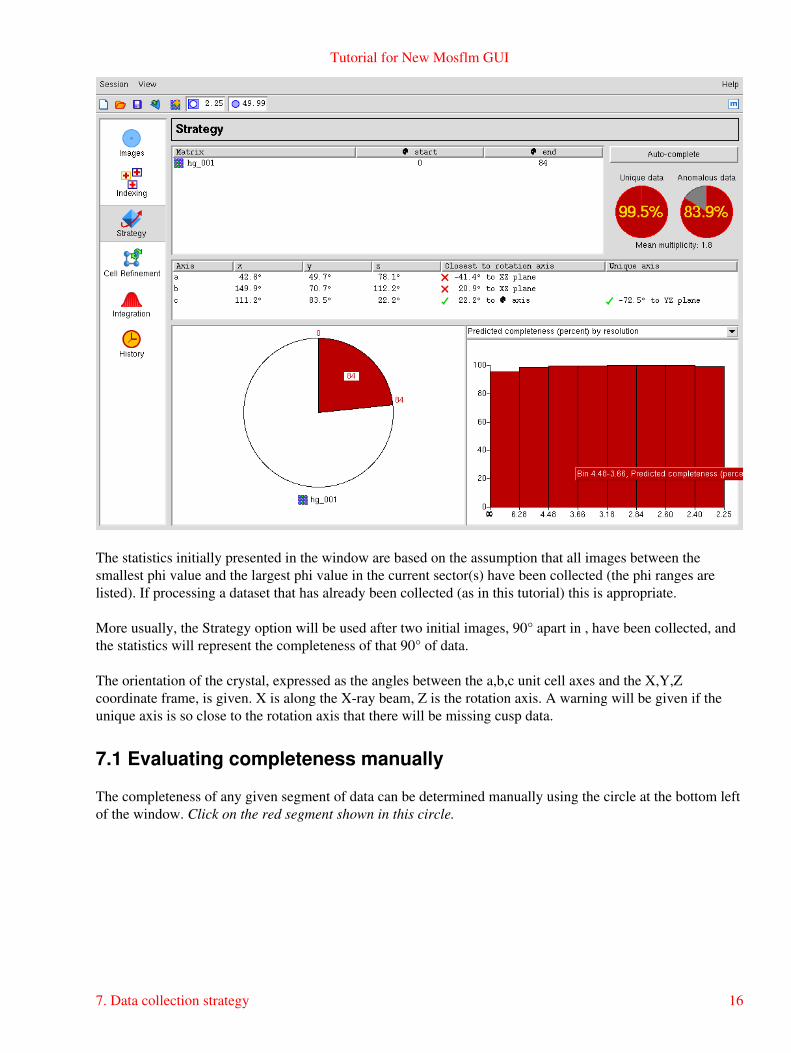
The statistics initially presented in the window are based on the assumption that all images between thesmallest phi value and the largest phi value in the current sector(s) have been collected (the phi ranges arelisted). If processing a dataset that has already been collected (as in this tutorial) this is appropriate.

More usually, the Strategy option will be used after two initial images, 90° apart in φ, have been collected, andthe statistics will represent the completeness of that 90° of data.

The orientation of the crystal, expressed as the angles between the a,b,c unit cell axes and the X,Y,Zcoordinate frame, is given. X is along the X-ray beam, Z is the rotation axis. A warning will be given if theunique axis is so close to the rotation axis that there will be missing cusp data.

7.1 Evaluating completeness manually

The completeness of any given segment of data can be determined manually using the circle at the bottom leftof the window. Click on the red segment shown in this circle.


7. Data collection strategy 16

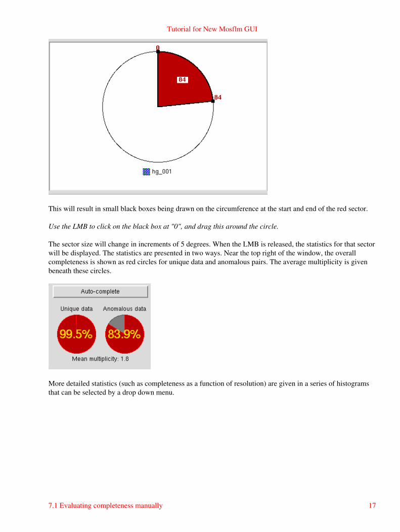
This will result in small black boxes being drawn on the circumference at the start and end of the red sector.

Use the LMB to click on the black box at "0", and drag this around the circle.

The sector size will change in increments of 5 degrees. When the LMB is released, the statistics for that sectorwill be displayed. The statistics are presented in two ways. Near the top right of the window, the overallcompleteness is shown as red circles for unique data and anomalous pairs. The average multiplicity is givenbeneath these circles.

More detailed statistics (such as completeness as a function of resolution) are given in a series of histogramsthat can be selected by a drop down menu.


7.1 Evaluating completeness manually 17

7.2 Calculating a strategy automatically

Select the Auto-complete button to calculate a strategy automatically.

An "scd" (Strategy calculation data) popup window will appear:

If multiple matrices have been defined (for different sectors of data) then the appropriate one can be selected(if there is only one sector, this has no effect).

The total φ rotation to be used is normally calculated by MOSFLM based on the Laue group and the crystalorientation (Auto). However, it is sometimes possible to achieve a high completeness with a significantlysmaller total rotation (eg 60° in two 30° segments will typically give >94% completeness for orthorhombicspace groups) and this can be useful if radiation damage is a serious problem.

Total rotation angles of between 30° and 90° can be selected from the drop down list. The number ofsegments to be used can be set between 1 and 3.

Two check boxes follow. If the first is checked, then it is assumed that data corresponding to the φ range listedhave already been collected, and a collection scheme to complete the data will be calculated. Only check thisbox if these data have indeed been collected.

The second box should be checked if the anomalous signal is to be used. THIS IS IMPORTANT. The


7.2 Calculating a strategy automatically 18

optimum strategy is often different when maximising completeness of the anomalous data.

Choose the default values (Auto, 1 segment) but check the anomalous data box. Look at the various statisticspresented as bar charts.

In space group H3, if rotating around the c axis, a total rotation of 120° would be required to collect acomplete dataset (ignoring any data lost in the cusp). Because the c axis is 22° away from the rotation axis inthis case, it is possible to collect very high completeness (for unique data) with a rotation much smaller thanthis.

Try to find the minimum total rotation that will give a dataset that is >95% complete for the unique data. Nowdo the same, but requiring >95% completeness for the anomalous data.

IGNORE SECTION 7.3 IF TIME IS SHORT

7.3 Calculating a strategy using multiple crystals

When collecting data from crystals that are very radiation sensitive, it may be necessary to use several crystalsto collect a complete dataset. If data have already been collected from several crystals, the GUI can be used tocalculate the best strategy for data collection from the current crystal. This is not implemented in the simplestway at present, but is usable. Assume that you have just indexed images from the latest crystal. Select theStrategy window.

Step 1. Set the phi range for the current crystal to zero (the current phi start, end are indicated in the topwindow). To do this, click anywhere in the red sector corresponding to the current phi range. Black squareswill appear at the phi start/end positions. Click LMB on either of these and drag it onto the other one so thatthe phi range becomes zero. (You cannot enter phi values in the top window).

Known bug. It is only possible to move the phi values in steps of 5°. If the initial value is not a multiple of 5°degrees, the first new value caused by dragging the mouse will be a multiple of 5° and further steps will be inmultiples of 5°. This means that in neither the start nor the final phi values are multiples of 5° then it will notbe possible to reset the phi range to zero, just reset it to the smallest possible value.

Step 2. Use the "Add Matrix" icon to read in the matrix file for the segment of data that has already beencollected. Make sure that this matrix has a unique name. When accepted, a new circle, with the matrix nameunderneath, will be displayed in the lower central window. In order to set the phi range for the data collectedfrom this crystal, select that matrix (by clicking on the circle above it) and set the phi values graphically byholding down the Ctrl key and positioning the mouse anywhere within the central lower window. A solid linewith a phi value attached will appear in the circle. Press the LMB to define the starting phi (as a multiple of5°) and drag the mouse to sweep out the phi range for this segment of data. Again, this can currently only beset in multiples of 5°.

Repeat Step 2 for any other segments of data that have already been collected.

The top window will display the matrix name and the phi start/end values for all segments of data entered.

Step 3. When all the data have been entered, click on the matrix name of the current crystal in the lowercentral window. Then select "Auto-complete". In the window that appears (see 7.2) select a total rotationrange for the current crystal. Normally the number of segments will be left at one, but if a rotation range ofabove 40° is chosen it might be worth trying 2 segments.


7.3 Calculating a strategy using multiple crystals 19

Then check the box "Include existing sectors". Then select OK. The best sector (of the specified phi width)will be chosen for the current crystal to get maximum completeness. Other sectors can be tried by draggingthe phi start/end values in the graphical phi range display.

Known bug. The information on data collected already is not saved when the Strategy window is left, and soif multiple crystals are being used, this information will have to be entered separately for each crystal.

7.4 Calculating a suitable oscillation angle

To calculate the maximum possible oscillation angle while avoiding spatial overlaps, click on the "Check foroverlaps" button. A popup window will appear, from which the option to calculate the maximum oscillationangle (as a function of &phi) or check how many overlaps will occur for different (user selected) oscillationangles. The results are plotted in the same pane as the histograms for the strategy calculations. Note that theoverlap calculation is based on the current values for the mosaic spread and spot separation, and can be verysensitive to these values.

8. Cell refinement

It is important to determine the cell parameters accurately before integrating the images. Although the unitcell is refined as part of the autoindexing, providing the diffraction extends beyond ~3.5Ãσ resolution it ispossible to obtain more accurate cell parameters using a procedure known as post-refinement. This procedurerequires the integration of a series of images in ideally two or more separate segments at widely different φvalues. The distribution of the intensity of partially recorded reflections over the images on which they occuris used to refine the unit cell, crystal orientation and mosaic spread.

Select the "Cell Refinement" icon


7.4 Calculating a suitable oscillation angle 20

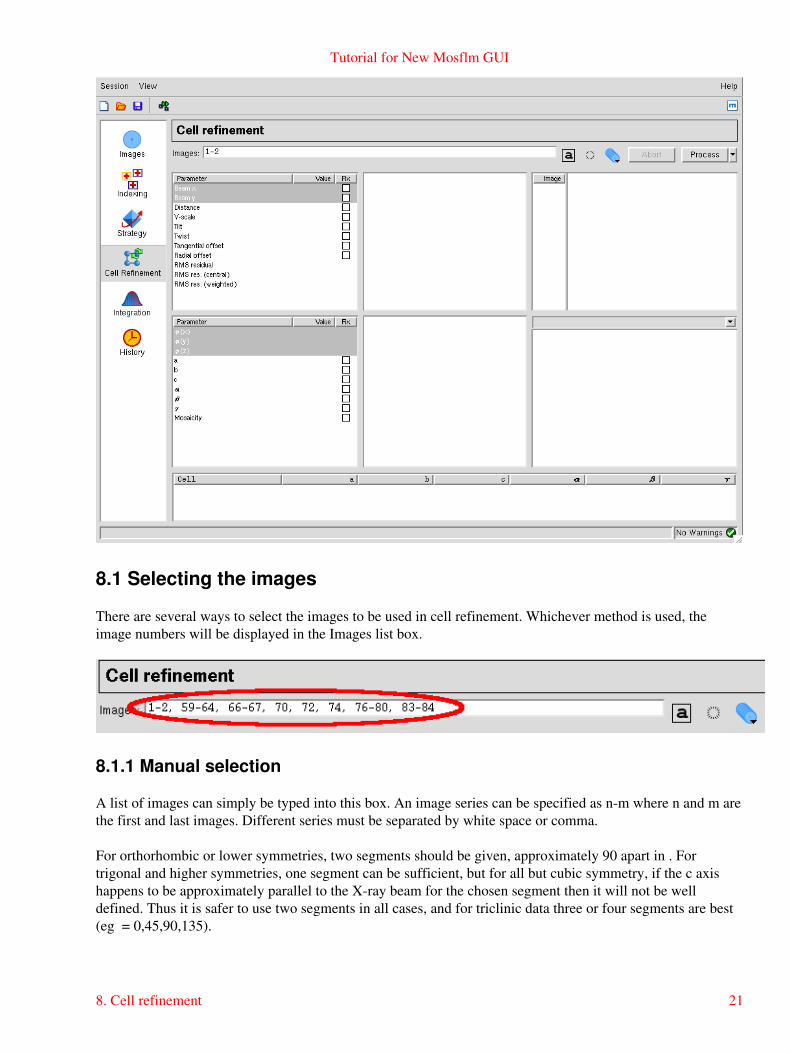
8.1 Selecting the images

There are several ways to select the images to be used in cell refinement. Whichever method is used, theimage numbers will be displayed in the Images list box.

8.1.1 Manual selection

A list of images can simply be typed into this box. An image series can be specified as n-m where n and m arethe first and last images. Different series must be separated by white space or comma.

For orthorhombic or lower symmetries, two segments should be given, approximately 90 apart in φ. Fortrigonal and higher symmetries, one segment can be sufficient, but for all but cubic symmetry, if the c axishappens to be approximately parallel to the X-ray beam for the chosen segment then it will not be welldefined. Thus it is safer to use two segments in all cases, and for triclinic data three or four segments are best(eg φ = 0,45,90,135).


8. Cell refinement 21

The number of images that should be included in each segment depends on the mosaic spread and oscillationangle. A reasonable number is 2*(mosaic spread/oscillation angle +1). MOSFLM will automatically selecttwo appropriate segments (for monoclinic/triclinic systems you may wish to add additional segments)

8.1.2 Automatic selection

Selecting the "Automatically select images" icon will select a suitable set of images.

8.1.3 Graphical selection

The graphical selection tool is the most powerful way of selecting images. Selecting this icon will give a newwindow:

Images can be selected by clicking in the "Use" checkbox in the list of images, or by using the mouse to draga selection of images from the sector displayed. The other icons allow the sector to be zoomed in or out andthe viewed area to be moved to make the selection easier (these icons do not work in iMosflm 0.4.5 andgenerate tcl errors so do not use them unless you have iMosflm 0.5.1 or later).


8.1.1 Manual selection 22

The final two icons fit the segment display to fit the window as either a full circle or a quadrant.

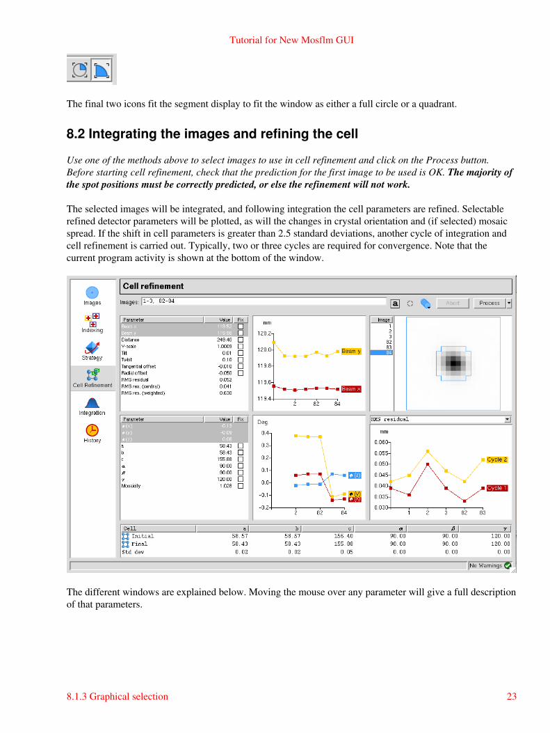
8.2 Integrating the images and refining the cell

Use one of the methods above to select images to use in cell refinement and click on the Process button.Before starting cell refinement, check that the prediction for the first image to be used is OK. The majority ofthe spot positions must be correctly predicted, or else the refinement will not work.

The selected images will be integrated, and following integration the cell parameters are refined. Selectablerefined detector parameters will be plotted, as will the changes in crystal orientation and (if selected) mosaicspread. If the shift in cell parameters is greater than 2.5 standard deviations, another cycle of integration andcell refinement is carried out. Typically, two or three cycles are required for convergence. Note that thecurrent program activity is shown at the bottom of the window.

The different windows are explained below. Moving the mouse over any parameter will give a full descriptionof that parameters.


8.1.3 Graphical selection 23

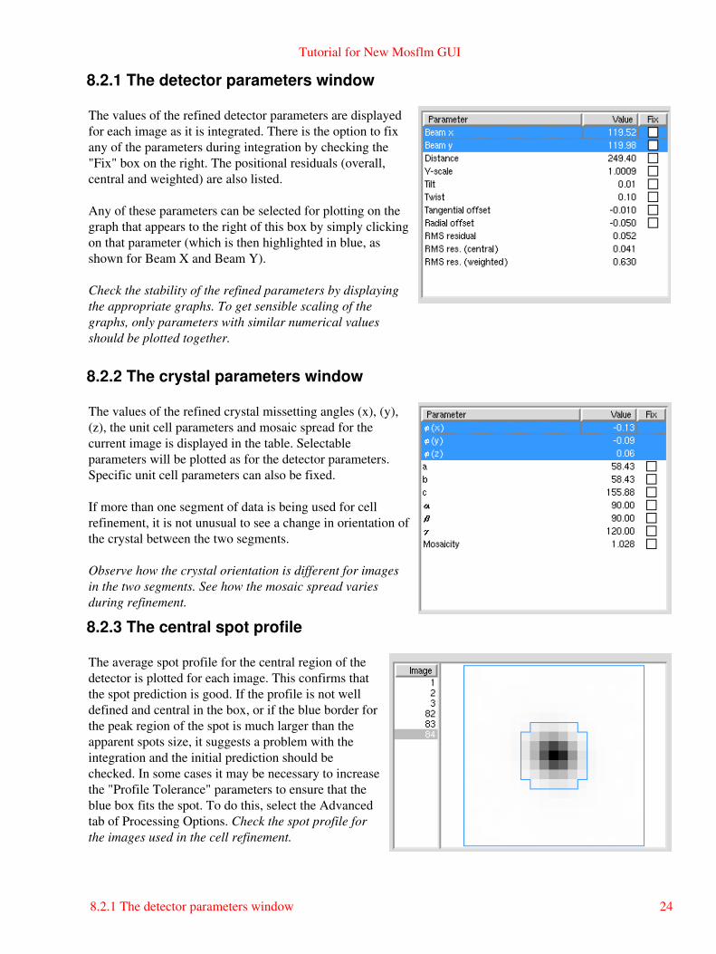
8.2.1 The detector parameters window

The values of the refined detector parameters are displayedfor each image as it is integrated. There is the option to fixany of the parameters during integration by checking the"Fix" box on the right. The positional residuals (overall,central and weighted) are also listed.

Any of these parameters can be selected for plotting on thegraph that appears to the right of this box by simply clickingon that parameter (which is then highlighted in blue, asshown for Beam X and Beam Y).

Check the stability of the refined parameters by displayingthe appropriate graphs. To get sensible scaling of thegraphs, only parameters with similar numerical valuesshould be plotted together.

8.2.2 The crystal parameters window

The values of the refined crystal missetting angles φ(x), φ(y),φ(z), the unit cell parameters and mosaic spread for thecurrent image is displayed in the table. Selectableparameters will be plotted as for the detector parameters.Specific unit cell parameters can also be fixed.

If more than one segment of data is being used for cellrefinement, it is not unusual to see a change in orientation ofthe crystal between the two segments.

Observe how the crystal orientation is different for imagesin the two segments. See how the mosaic spread variesduring refinement.

8.2.3 The central spot profile

The average spot profile for the central region of thedetector is plotted for each image. This confirms thatthe spot prediction is good. If the profile is not welldefined and central in the box, or if the blue border forthe peak region of the spot is much larger than theapparent spots size, it suggests a problem with theintegration and the initial prediction should bechecked. In some cases it may be necessary to increasethe "Profile Tolerance" parameters to ensure that theblue box fits the spot. To do this, select the Advancedtab of Processing Options. Check the spot profile forthe images used in the cell refinement.


8.2.1 The detector parameters window 24

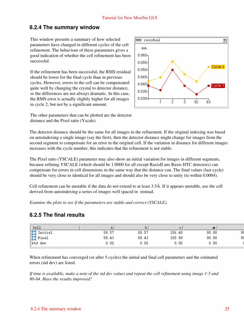
8.2.4 The summary window

This window presents a summary of how selectedparameters have changed in different cycles of the cellrefinement. The behaviour of these parameters gives agood indication of whether the cell refinement has beensuccessful.

If the refinement has been successful, the RMS residualshould be lower for the final cycle than in previouscycles. However, errors in the cell can be compensatedquite well by changing the crystal to detector distance,so the differences are not always dramatic. In this case,the RMS error is actually slightly higher for all imagesin cycle 2, but not by a significant amount.

The other parameters that can be plotted are the detectordistance and the Pixel ratio (Yscale).

The detector distance should be the same for all images in the refinement. If the original indexing was basedon autoindexing a single image (say the first), then the detector distance might change for images from thesecond segment to compensate for an error in the original cell. If the variation in distance for different imagesincreases with the cycle number, this indicates that the refinement is not stable.

The Pixel ratio (YSCALE) parameter may also show an initial variation for images in different segments,because refining YSCALE (which should be 1.0000 for all except RaxisII ans Raxis HTC detectors) cancompensate for errors in cell dimensions in the same way that the distance can. The final values (last cycle)should be very close to identical for all images and should also be very close to unity (to within 0.0004).

Cell refinement can be unstable if the data do not extend to at least 3.5Å. If it appears unstable, use the cellderived from autoindexing a series of images well spaced in φ instead.

Examine the plots to see if the parameters are stable and correct (YSCALE).

8.2.5 The final results

When refinement has converged (or after 5 cycles) the initial and final cell parameters and the estimatederrors (std dev) are listed.

If time is available, make a note of the std dev values and repeat the cell refinement using image 1-5 and80-84. Have the results improved?


8.2.4 The summary window 25

9. Integration

The accurate cell parameters are now used in the integration. Note that although the images are integratedduring the cell refinement, the intensities are not saved and no MTZ file is generated.

It is good practice to start by integrating a block of about ten images, to check that the parameters do not needfurther adjustment. MOSFLM will generate warning messages after integration if there are any difficulties,and it may be possible to improve the situation by changing some of the default parameters (see 11).

9.1 Image selection

Image selection is performed in exactly the same way as in the cell refinement. In this case, the "Automatic"selection will simply include all images in the current sector.

Select images 1-10

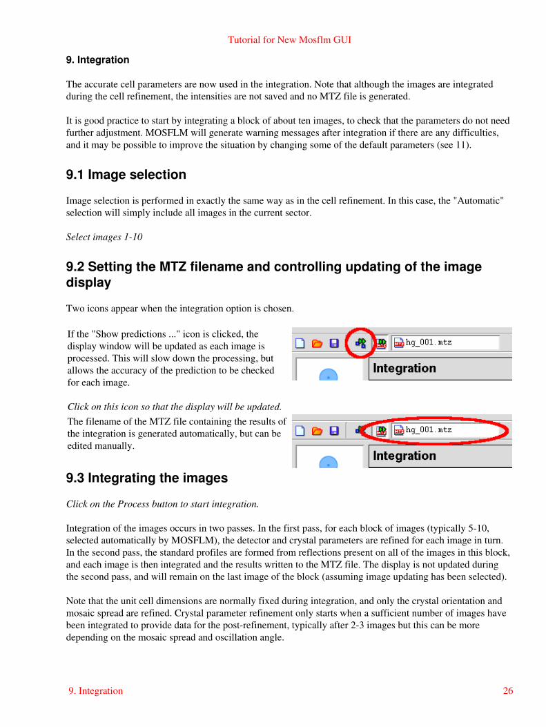
9.2 Setting the MTZ filename and controlling updating of the imagedisplay

Two icons appear when the integration option is chosen.

If the "Show predictions ..." icon is clicked, thedisplay window will be updated as each image isprocessed. This will slow down the processing, butallows the accuracy of the prediction to be checkedfor each image.

Click on this icon so that the display will be updated.The filename of the MTZ file containing the results ofthe integration is generated automatically, but can beedited manually.

9.3 Integrating the images

Click on the Process button to start integration.

Integration of the images occurs in two passes. In the first pass, for each block of images (typically 5-10,selected automatically by MOSFLM), the detector and crystal parameters are refined for each image in turn.In the second pass, the standard profiles are formed from reflections present on all of the images in this block,and each image is then integrated and the results written to the MTZ file. The display is not updated duringthe second pass, and will remain on the last image of the block (assuming image updating has been selected).

Note that the unit cell dimensions are normally fixed during integration, and only the crystal orientation andmosaic spread are refined. Crystal parameter refinement only starts when a sufficient number of images havebeen integrated to provide data for the post-refinement, typically after 2-3 images but this can be moredepending on the mosaic spread and oscillation angle.


9. Integration 26

9.4 Parameter display windows

As described in 8.2, the refined detector and crystal parameters will be displayed in tables and selectedparameters will be plotted in graphs. The average spot profile for each image will also be displayed.

The size of these graphs (and the profile) can be expanded to fill the whole window by holding down "shift"and clicking LMB anywhere in the graph window. A second "shift+click" will revert the graph to the originalsize.

In addition to these windows, there are windows that tabulate and plot (as a function of image number) themean I/σ(I) for profile fitted and summation integration intensities. The overall values and the values for thehighest resolution bin are given.

A display of the standard profiles for different regions of the detector is also provided. Poor profiles are"averaged", by including reflections from inner regions of the detector, and the display indicates whichprofiles have been averaged and allows inspection of the original "unaveraged" profile (providing there weresufficient spots in that region to allow formation of a profile).

The profiles should be checked to see that they are well defined and centred within the box. (Poorly defined,diffuse or non-centred profiles may suggest that the prediction is not very good, in which case this should bechecked on the image).

It may be useful to expand the standard profiles to fill the window using "Shift + mouse click" in the profileswindow).

Finally, the lower left window plots I/σ(I) as a function of resolution for any selected image.

Different parameters can be plotted by selecting the right or left pointing arrows.


9.4 Parameter display windows 27

9.5 Integrating the whole dataset

Assuming that everything looks OK, the entire dataset can now be integrated. However, it is stronglyrecommended that Project/Crystal/Dataset names are assigned first. These are written to the output MTZ fileand used by downstream programs, in particular SCALA will use this information when deciding whichimages belong to the same dataset.

Select "Experiment settings" from the "View" drop down menu (2.1) to define these names and optionallygive a title for the MTZ file.

Select images 1-84 and click on "Process".

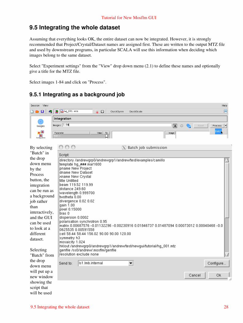
9.5.1 Integrating as a background job

By selecting"Batch" inthe dropdown menuby theProcessbutton, theintegrationcan be run asa backgroundjob ratherthaninteractively,and the GUIcan be usedto look at adifferentdataset.

Selecting"Batch" fromthe dropdown menuwill put up anew windowshowing thescript thatwill be used


9.5 Integrating the whole dataset 28

to process theimages. Thisscript can beedited ifadditionalkeywords arerequired or ifsomeparametersare to bechanged. It ispossible toconfigure jobsubmissionfor remotemachines.

The logfilefor batchsubmissionjobs iswritten to the".mosflm"directory(created byimosflm if itdoes notexist) in yourhomedirectory.The MTZandSUMMARYfiles arewritten to thedirectory inwhichimosflm waslaunched.

9.6 Checking the integration

The detector and crystal parameter plots should be examined carefully to check for any instability in therefinement. If there are large and random variations in some parameters (eg the detector twist and tilt) then itmay be better to fix them and repeat the integration. Discontinuities due to blank images should also show up,and the offending images removed from the scaling run.

If adjacent spots are incompletely resolved on the detector, it may be possible to improve the processing byincreasing the PROFILE TOLERANCE parameters by 1-2%. These parameters can be set in the Advancedtab of the Processing Options menu (use View).


9.5.1 Integrating as a background job 29

9.7 Advanced features for integration

The "View"/"Processing options" drop down menu allows additional control over the integration. Parameterssuch as the minimum spot separation, resolution limits, block size, MTZ filename and BATCH ADD can bechanged in the Processing tab. In the Advanced tab, the measurement box parameters, profile tolerance andprofile averaging parameters can be set.

Additional MOSFLM parameters will be added based on user requests.

10. Running Pointless to check the symmetry

Once the images have been integrated (even a subset of the whole dataset) the program POINTLESS can berun determine the true Laue symmetry and try to determine the spacegroup.

Select the QuickSymm button. A summary of the Pointless results as shown below will appear in a browserwindow. (Note that the environment variable CCP4_BROWSER must be set to a web browser that is installedon your machine for this to work).


9.7 Advanced features for integration 30

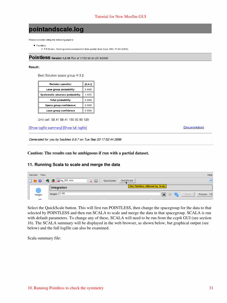
Caution: The results can be ambiguous if run with a partial dataset.

11. Running Scala to scale and merge the data

Select the QuickScale button. This will first run POINTLESS, then change the spacegroup for the data to thatselected by POINTLESS and then run SCALA to scale and merge the data in that spacegroup. SCALA is runwith default parameters. To change any of these, SCALA will need to be run from the ccp4i GUI (see section16). The SCALA summary will be displayed in the web browser, as shown below, but graphical output (seebelow) and the full logfile can also be examined.

Scala summary file:


10. Running Pointless to check the symmetry 31

Part of the Scala graphical output:


11. Running Scala to scale and merge the data 32

12. History and mosflm logfile

Selecting History allows the history of the session to be examined, or, by selecting the Log tab, the fullmosflm.lp file can be viewed.

The History has a tree structure, and will show when various parameters have been changed. It is possible to"Undo" some of the actions shown in the History, although this feature has not been extensively tested.

13. Warning Messages

As already mentioned in sections 3 and 9, warning messages are generated by MOSFLM during processingand the abbreviated messages can be obtained by clicking on the "Warnings" icon (see 3). The full warningswill eventually be available via the GUI, but at present it is necessary to look at the mosflm.lp file (or the Logfile via the History) to get full details and suggestions.

NOTE This is the end of the part of the tutorial which deals directly with iMosflm (but see section 19which has some suggestions for further work if you have time). The remainder of this document dealswith integrating and scaling data with MOSFLM and Scala via the CCP4i user interface, examiningthe traditional MOSFLM SUMMARY file with the CCP4 utility loggraph.

There are also two appendices, one which contains a shell script for running MOSFLM as a traditionalbatch job, and one which gives an example of using the TESTGEN option in MOSFLM in order towork out the optimal oscillation angle for the images in the data collection.14. Using the CCP4i GUI to integrate images

By selecting to submit a background processing job (see 9.5.1) it is possible to use the CCP4i GUI to integratethe images. As described in 9.5.1, a window with the MOSFLM commands will appear. These commandsshould be pasted into a file (eg hg.sav). It is also necessary to save the orientation matrix to a file. To do this,select the Images window and double click on the matrix. A window will pop up which allows the matrix tobe saved to a file.

> ccp4i

Select "Directories & ProjectDir" (Top left)

In the new window, select "Add project"

Type in the Project and the full directory path (uses directory)

Select this project from "Project for this session..."

Select "Apply and Exit" ... Dismiss the warning message that comes up.

Select "Data reduction" from the pull down menu of modules (orange bar at top left; if you haven't usedCCP4i before, it probably says "Coordinate utilities", but the state is saved from the previous session) so itmay be different.

Select "Integrate Images" (the first option).

A window will be displayed which allows you to set up a batch MOSFLM job.


12. History and mosflm logfile 33

You need to provide the information stored in the "save" file.

Give a job title. On the next line ("Load parameters from command file") select "browse" and locate the ".sav"file that you saved from the MOSFLM session. Once you have selected the file, click on "Load parametersfrom command file" and the information will be read from the save file.

You should then supply a "Crystal" and a "Dataset" names.

Then in the box headed "Images to Integrate", click on "Add processing run", and in the resulting block clickon "Add block of images". Supply the number of the first and last image (1 and 84). The job can then besubmitted.

15. The MOSFLM SUMMARY file

MOSFLM produces a summary file listing refined parameters for each image, and when using the new GUIthis file will be called always be called SUMMARY (and will be overwritten by any subsequent job unlessrenamed). This contains the same information as the plots produced by the new GUI, but in addition it lists thenumber of "badspots" and overloads, which are not yet available in the new GUI.

This can be inspected graphically with the CCP4 program "loggraph":

> loggraph SUMMARY

This is very useful to identify "rogue" images (with unusually high positional residual, or low I/σ(I)). If youfind any, read that image into MOSFLM and see what is wrong with it.

If you have done more than one integration run during your MOSFLM session, you will find multiple entriesof the tables. Look at the last set for integration of the 84 images.

Click on the "Refined detector parameter" tables and check on the stability of parameters like the TILT andTWIST of the detector (units are hundredths of a degree) and, for Mar Research (or DIP) image plate data, thedistortion parameters ROFF and TOFF (units are mm). If they are varying a lot (more than 20 forTWIST/TILT) or 0.15 for ROFF/TOFF then it is probably a good idea to fix these parameters at the averagevalue (or the known values for this detector, if they are available) (see section 8.2.1).

Click on the "Post refinement" table and check the missets...it does not matter if they change slowly and by anamount (per image) that is less than 0.1*mosaic spread. If they are changing more than this then there couldbe a problem with processing the data (there is not much you can do about this).

Check how the mosaic spread is changing. If it is unstable, or if you think it is not refining to sensible values(as judged by looking at the prediction) then you can fix the input value in the same way as the detectorparameters (see section 8.2.2).

BADSPOTS AND OVERLOADS

The program will set a rejection flag for those reflections that fail certain tests, for example too muchvariation in the background level, a poor profile fit, an intensity that is very negative (more than 5 sds), a veryhigh gradient for the background plane. These reflections are called "Bad spots" and they are listedindividually for each image in the mosflm.lp file, together with the reason for flagging them. The number ofbad spots is also written to the summary file. Generally there should be very few (5-10) bad spots on each


14. Using the CCP4i GUI to integrate images 34

image. If there are more, it could be because the backstop shadow is not correctly allowed for (consider usingthe NULLPIX keyword).

There should also be very few overloaded reflections on each image. If there are a lot, then a separate lowresolution data collection pass should be made with a much shorter exposure time.

IMPORTANT: Both "Bad spots" and "Overloads" are written to the output MTZ file, but will be rejected bydefault by SCALA. The intensity of overloaded reflections is estimated by profile fitting that part of the spotthat is not saturated. To include these reflections in the final merged data, use the ACCEPT keyword inSCALA.

16. Scaling data with CCP4i

> ccp4i

Select "Directories & ProjectDir" (Top left) In the new window, select "Add project"

Type in the Project and then the full directory path (uses directory) or use the "Browse.." button to select it.

Select this project from "Project for this session..."

Select "Apply and Exit" ... Dismiss the warning message that comes up.

Select "Data reduction" from the pull down menu of modules (orange bar at top left)

Select "Scale and Merge intensities"

In the window that appears:

Give a job title (top line)1. Click on the box next to "Separate anomalous pairs for merging/output" (the crystals have beensoaked in a mercury compound).

2.

In the next orange bar (line starts "MTZ in") select Browse and select the MTZ file output byMOSFLM (probably called hg_001.mtz) Select "OK"

3.

In the next orange box ("Estimated number of residues...") Enter 91

Under "Scaling Protocol":

4.

From the pull down menu on the line starting "Scale", select "On rotation axis with secondary beamcorrection"

5.

On the same line, from the pull down menu select "Isotropic B" (default is no B-factor correction).6. At bottom of window, from pull down menu named "Run" select "Run and view command file"

This will put up a new window showing the command file for running the "Sort" step, select"Continue". After a brief pause it will show the command file for running SCALA. (This can beedited before submitting the job). Select "Continue"

In the main window, it will show that the SCALA job is running.

When SCALA has finished, the command file for running the TRUNCATE step will appear...select"Continue".

7.


BADSPOTS AND OVERLOADS 35

When TRUNCATE has run, the main window will say "FINISHED".

At that point, select the pull down menu "View files from job" and select "View log graphs". This willgive you the same graphs are running loggraph on the SCALA logfile. To look at the logfile itself (egthe overall merging statistics) select "View logfile" and it will appear in a new window.

When SCALA has finished, the command file for running the TRUNCATE step will appear...select"Continue".

16.1 Looking at the SCALA output

The simplest way to look at the output from SCALA is to use loggraph on the log file (or via the CCP4i GUI).This can display many different graphs.

Use "Scales vs rotation range" to check for smooth variation in the scale factor. Check the variation in Bfactor with image, and if there is no real variation it is best to turn off the B-factor refinement.

Use the "Analysis against batch" to detect "bad" images (high R-factor, large number of rejected spots).

Check the "Analysis against resolution" Fractional bias to see if there is any indication of "Partial bias" (Anegative partial bias will result if the mosaic spread is underestimated, or if there is a lot of diffuse scatter. TheTAILS correction can be used in SCALA to correct for diffuse scatter.

The Fractional bias should be less than 1-2%, although it will often exceed this for weak data (eg in the highresolution bins).

The "Axial reflections" graphs are useful for detecting systematic absences, which can be used to identify thetrue space group.

It can also be useful to look at the SCALA logfile itself, in particular the table giving statistics as a function ofresolution. The effective resolution limit of the data can be determined by looking at the Mn(I)/sd column(this is the mean I/σ(I) AFTER merging symmetry mates, and is the best indicator of data quality). This tablealso shows shell and cumulative R-factors.

The Mn(I)/sd values depend on having realistic values of the standard deviations (errors) in the intensities. Asthe values that come from MOSFLM are always underestimates of the true error, these values are scaled up inSCALA using a two-term correction:

sdcorrected = SdFac * Sqrt[sd(I)**2 + SdB*LP*I + (SdAdd*I)**2]

Here "SdFac" is an overall scale factor, and "SdB" and "SdAdd" are intensity dependent factors.

SCALA will automatically work out a suitable value for all three parameters, in order to make the mean valueof (observed scatter)/(sdestimate) equal to 1.0, where "observed scatter" is the differences between anindividual estimate of intensity and the mean of all other estimates (from symmetry mates).

This table comes under the heading:

ANALYSIS OF STANDARD DEVIATIONS


16. Scaling data with CCP4i 36

in the SCALA logfile.

Can you identify a bad image in this dataset ? Can you work out why it is bad ?

(Clue...the image headers contain quite a lot of information that is not used by MOSFLM, including the dateand time that the image was collected).

You can exclude a given batch from the scaling using the EXCLUDE keyword:

RUN ALL EXCLUDE imagenumber

In this case, runnumber will be "1".

Rerun the scaling, SENDING THE OUTPUT TO A NEW LOGFILE, excluding this image, and see the effecton the heights in the anomalous Patterson (in the logfile). DO NOT repeat the integration. In the commandfile, uncomment the line (near the top) "goto scala" so it skips the integration part.

17. Changing the symmetry

From the list of options at the left hand side of the main window, select "Sort/Reindex MTZ files" In the newwindow give a new title, eg reindex as H32

Click on the Box "Change space group or reindex reflection"

Use the "browse" option to select the input MTZ file (First orange bar), the output filename will be generatedautomatically (but you can change it).

Under "Reindex details"

In the last option "Reduce to asymmetric unit for space group ..." (which is the one selected by default) enterH32 in the box.

Select "Run" from "Run" pull down menu.

The go back to the scaling window, and select the new MTZ file (reindexed) as the input for scaling (use"Browse"). CHANGE THE JOB TITLE

Then select "RUN"

The scaling will now be performed in space group H32. Look at the merging statistics in the logfile, inparticular the multiplicity weighted R-factor, called Rmeas in the logfile.

18. Looking at the TRUNCATE output

The TRUNCATE program converts intensities to amplitudes, and also compiles some useful statistics. The socalled "cumulative intensity statistics" tabulated by Truncate (and plotted by loggraph) provides the only pointat which you will be able to detect merohedral twinning (when the two lattices of the twin components exactlyoverlap, and every measured intensity is actually the sum of two intensities).


16.1 Looking at the SCALA output 37

For a good dataset, the observed distribution should be within 1% of the theoretical distribution. Is this thecase for this data ?

19. If you have time ....

19.1 Different mosaic spreads

Try repeating the processing with the mosaic spread set to a value 25% smaller than the refined one and fix itby checking the "Fix" box in the Integration window.

Can you tell from the merging statistics if this data is better ?

19.2 Checking up on outliers

SCALA writes a file called ROGUES which lists reflections which show very poor agreement betweensymmetry mates, or which are implausibly large.

Look in this file (it is ASCII), and try to work out why this has happened. The ROGUES file gives you theimage (Batch) on which the reflections have been recorded (for partials, this is the image nearest the centre ofthe reflection, so you may need to look on the preceding and following image as well). Select a reflectionwhich shows very poor agreement with its symmetry mates (A value greater than 10 in the DelI/sd column inthe ROGUES file). Read in the offending image using "Read image" in the Main menu. Predict thereflections, then use "Find hkl" to locate the offending reflection in the image (you must give the measuredindices, the first set of values in the ROGUES file, when doing this). See if there is anything odd about thespot. Remember to check adjacent images for partials.

19.3 How accurate does the unit cell have to be ?

Try changing the cell parameters by (say) 1.0% and integrate the images again. What is the effect on themerging statistics ?

Appendix I

A command script for running MOSFLM, using the "save" file from the old GUI or from backgroundprocessing of the new GUI. Note that keyworded input for MOSFLM and other CCP4 programs iscase-insensitive apart from file and directory names.

#!/bin/csh -fv # # Maxinf Workshop on Data Processing, Cambridge, December 2002 # # A generic command file for processing data. For completeness, # I have left in the steps that calculate an anomalous Patterson map. # Andrew Leslie # Variables to generate unique filenames. Change the "job" variable # if processing multiple times, eg with different mosaic spread values. # "scr" defines a scratch disk #


18. Looking at the TRUNCATE output 38

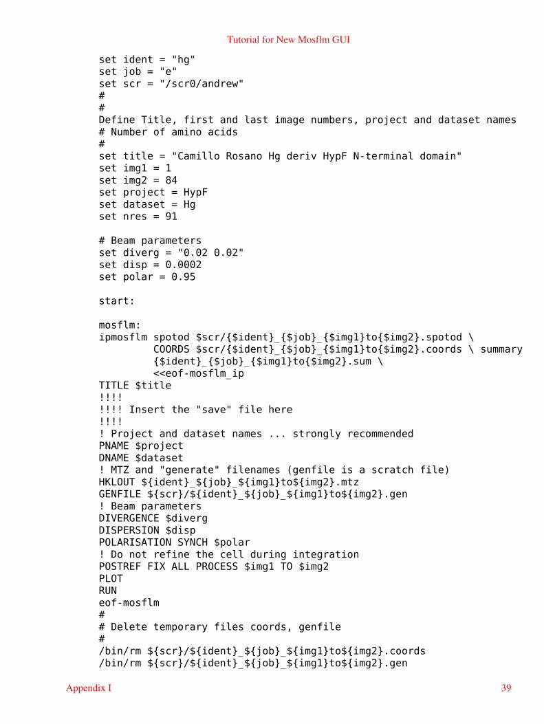
set ident = "hg" set job = "e" set scr = "/scr0/andrew" # #Define Title, first and last image numbers, project and dataset names# Number of amino acids # set title = "Camillo Rosano Hg deriv HypF N-terminal domain" set img1 = 1 set img2 = 84 set project = HypF set dataset = Hg set nres = 91

# Beam parameters set diverg = "0.02 0.02" set disp = 0.0002 set polar = 0.95

start:

mosflm: ipmosflm spotod $scr/{$ident}_{$job}_{$img1}to{$img2}.spotod \ COORDS $scr/{$ident}_{$job}_{$img1}to{$img2}.coords \ summary {$ident}_{$job}_{$img1}to{$img2}.sum \

<<eof-mosflm_ip TITLE $title!!!!!!!! Insert the "save" file here !!!!! Project and dataset names ... strongly recommended PNAME $project DNAME $dataset ! MTZ and "generate" filenames (genfile is a scratch file) HKLOUT ${ident}_${job}_${img1}to${img2}.mtz GENFILE ${scr}/${ident}_${job}_${img1}to${img2}.gen ! Beam parametersDIVERGENCE $diverg DISPERSION $disp POLARISATION SYNCH $polar ! Do not refine the cell during integration POSTREF FIX ALL PROCESS $img1 TO $img2 PLOT RUN eof-mosflm # # Delete temporary files coords, genfile #/bin/rm ${scr}/${ident}_${job}_${img1}to${img2}.coords /bin/rm ${scr}/${ident}_${job}_${img1}to${img2}.gen


Appendix I 39

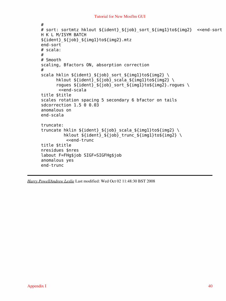
# # sort: sortmtz hklout ${ident}_${job}_sort_${img1}to${img2} <<end-sort H K L M/ISYM BATCH${ident}_${job}_${img1}to${img2}.mtz end-sort # scala: # # Smoothscaling, Bfactors ON, absorption correction #scala hklin ${ident}_${job}_sort_${img1}to${img2} \ hklout ${ident}_${job}_scala_${img1}to${img2} \ rogues ${ident}_${job}_sort_${img1}to${img2}.rogues \

<<end-scala title $title scales rotation spacing 5 secondary 6 bfactor on tailssdcorrection 1.5 0 0.03 anomalous on end-scala

truncate: truncate hklin ${ident}_${job}_scala_${img1}to${img2} \ hklout ${ident}_${job}_trunc_${img1}to${img2} \

<<end-trunc title $title nresidues $nres labout F=FHg$job SIGF=SIGFHg$job anomalous yesend-trunc

Harry PowellAndrew Leslie Last modified: Wed Oct 02 11:48:30 BST 2008


Appendix I 40

mailto:[email protected]

mailto:[email protected]

tutorial for new mosflm gui - bgulifeserv.bgu.ac.il/wb/zarivach/media/documentation/imosflm... ·...

Documents