Tutorial  6:  Vasp  Calcula1ons  for  Ab  Ini'o  Molecular  Dynamics  

Deyu  Lu  and  Neerav  Kharche  

Worhshop  on  “Theory  and  Computa1on  for  Interface  Science  and  Catalysis:  Fundamentals,  Research  and  Hands  

on  Engagement  using  VASP”  Nov.  3  –  7,  2014  

Outline  

•  Basic  of  molecular  dynamics  

•  Ab  ini'o  molecular  dynamics  

•  AIMD  run  for  16  H2O  cell  

•  Data  analysis  of  precomputed  32  H2O  cell  

Molecular  dynamics  

1.  Alder,  B.  J.  and  Wainwright,  T.  E.  J.  Chem.  Phys.  27,  1208  (1957)  2.  Alder,  B.  J.  and  Wainwright,  T.  E.  J.  Chem.  Phys.  31,  459  (1959)  3.  Rahman,  A.  Phys.  Rev.  A136,  405  (1964)  4.  S1llinger,  F.  H.  and  Rahman,  A.  J.  Chem.  Phys.  60,  1545  (1974)  5.  McCammon,  J.  A.,  Gelin,  B.  R.,  and  Karplus,  M.  Nature  (Lond.)  267,  585  (1977)    

"for  the  development  of  mul1scale  models  for  complex  chemical  systems".  

•  protein  folding,    •  catalysis,  •  electron  transfer,    •  drug  design  •  …  

Winners  of    Nobel  Prize  in  Chemistry  2013  

Mar1n  Karplus   Michael  Levia   Arieh  Warshel  

Ergodicity  Ensemble  average  

   Average  over  all  possible  states  of  the  system  in  the  phase  space    

Time  average      Average  over  a  sufficiently  long  1me  

Aens= dpN drNρ rN , pN( )A rN , pN( )∫∫ A

time= lim

τ→∞

1τ dt

0

τ

∫ A rN (t), pN (t)( )

Ergodicity  If  one  allows  the  system  to  evolve  in  1me  indefinitely,  that  system  will  eventually  pass  through  all  possible  states.  

The  ergodic  hypothesis  states          Ensemble  average  =  Time  average  

Aens= A

time

Integra1on  of  equa1ons  of  mo1on  

•  Verlet  algorithm  –  the  error  in  new  posi1on  is  O(Δt4)  –  does  not  use  the  velocity  to  compute  the  new  posi1on  –  the  velocity  can  be  derived  with  an  error  of  O(Δt2)  

•  Leap  frog  algorithm  –  evaluates  the  veloci1es  at  half-­‐integer  1me  steps  –  Uses  veloci1es  to  compute  new  posi1ons  

•  Velocity-­‐corrected  Verlet  algorithm  –  the  error  in  both  the  posi1ons  and  veloci1es  is  O(Δt4)  –  requires  posi1ons  and  forces  at  t+Δt  to  update  velocity  

•  Higher-­‐order  schemes  

F =m !!rNewton’s  equa1on  of  mo1on:  

Verlet  Algorithm    

rn+1 = rn + vnΔt + 12Fnm

"

#$

%

&'Δt2 +O(Δt3)

rn−1 = rn − vnΔt + 12Fnm

#

$%

&

'(Δt2 −O(Δt3)Posi@on  at  step  n-­‐1:  

Posi@on  at  step  n+1:  

Sum  of  the  two  term:  propagate  posi@on   rn+1 = 2rn − rn−1 +

Fnm

"

#$

%

&'Δt2 +O(Δt 4 )

Do  a  subtrac@on  v  is  one  step  behind  

vn =rn+1 − rn−12Δt

+O(Δt2 )

Common  thermal  dynamic  ensembles  •  Microcanonical  ensemble  (NVE)  

–  Isolated  –  Total  energy  E  is  fixed  –  Every  accessible  microstate  has  equal  probability  

•  Canonical  ensemble  (NVT)  –  The  system  can  exchange  energy  with  a  heat  bath  –  T  is  constant  –  Probability  of  finding  the            system  at  state  i  

•  Isobaric-­‐isothermal  ensemble  (NPT)  –  Both  P  and  T  are  constant  

•  Grand  canonical  ensemble  (µVT)  

pi =e−Ei /kBT

e−Ei /kBTi∑

classical  

Microcanonical  ensemble  

v  v  

•  Ini1alize  r0  and  v0  

•  Calculate  force  

•  Integrate  the  equa1on  of  mo1on  

•  Update  r  and  v      

Canonical  ensemble  (NVT)  

•  Berendsen  thermostat:  Velocity  rescaling  •  Anderson  thermostat:  Stochas1c  coupling  •  Nosé-­‐Hoover  thermostat:  Extended  Lagrangian  

P(p) = β2πm( )

3/2e−(βp

2 /2m)Maxwell-­‐Boltzmann  distribu1on:  

kBT =m vα2Temperature                                  kine1c  energy:    

EK = 32 NkBT

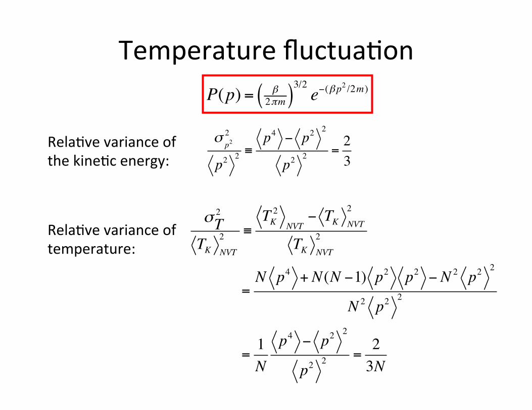
Temperature  fluctua1on  

Rela1ve  variance  of  the  kine1c  energy:  

P(p) = β2πm( )

3/2e−(βp

2 /2m)

Rela1ve  variance  of  temperature:    

σp22

p22 ≡

p4 − p22

p22 =

23

σT2

TK NVT

2 ≡TK

2

NVT− TK NVT

2

TK NVT

2

=N p4 + N(N −1) p2 p2 − N 2 p2 2

N 2 p2 2

= 1N

p4 − p2 2

p2 2 =2

3N

Berendsen  thermostat  

ΔT = 12

2mi (λvi )2

3NkBi=1

N

∑ − 12

2mivi2

3NkBi=1

N

∑

= (λ 2 −1) T (t)

λ = Tbath /T (t)

dTdt

=Tbath −T

τ

λ 2 =1+ Δtτ

TbathT

−1#

$%

&

'(

•  Not  real  canonical  ensemble,  although  close  

•  No  direct  proof  of  Maxwell-­‐Boltzmann  distribu1on  

Andersen  thermostat  •  Start  with  {r0N,  p0N}  and  integrate  the  equa1ons  of  mo1on  for  Δt.  

•  A  number  of  par1cles  are  selected  to  undergo  a  collision  with  the  heat  bath,  if  p>ν Δt.  

•  The  new  velocity  will  be  drawn  from  a  Maxwell-­‐Boltzmann  distribu1on  at  Tbath.  

ü  Andersen  thermostat  guarantees  the  canonical  distribu1on.  

x  The  stochas1c  collisions  destroy  the  correla1on  of  par1cle  veloci1es,  which  disturbs  dynamic  proper1es.  

Nosé-­‐Hoover  thermostat  

•  An  extended  Lagrangian  method.  •  Determinis1c  molecular  dynamics.  •  It  produces  a  canonical  due  to  heat  exchange  between  fic11ous  degree  of  freedom  and  real  system.  

•  s  is  a  scaling  factor  of  the  1me  step,  so  the  1me  step  fluctuates.    

H =pi2

2mis2 +U(r

N )+ ps2

2Qi=1

N

∑ + L Lnsβ

Ab  ini'o  molecular  dynamics  

In  general,  we  need  to  solve  

electronic  degree  of  freedom  

nuclear  degree  of  freedom  

Hamiltonian  containing  both  nuclear  and  electronic  degrees  of  freedom  

Born-­‐Oppenheimer  molecular  dynamics  the  adiaba@c  approxima@on  

separa@on  of  variables:  

•  Electrons   stay   in   the   adiaba1c   ground   state   at   any   instant   of  1me.  

•  Nuclei  move  on  the  ground  state  Born-­‐Oppenheimer  poten1al  energy  surface.  

•  It  a  good  approxima1on   if   the  energy  difference  between  the  electronic   ground   state   and   first   excited   state   is   large  compared  kBT.    

•  Minimiza1on  is  required  at  each  step  of  the  MD  simula1on  and  the  forces  are  computed  using  the  orbitals  thus  obtained.  

 Car–Parrinello  molecular  dynamics  •  The  coupling  between  nuclear  1me  evolu1on  and  electronic   minimiza1on   is   treated   efficiently   via  an  implicit  adiaba1c  dynamics  approach.  

•  A  fic11ous  dynamics  for  the  electronic  orbitals  is  invented   which,   given   orbitals   ini1ally   at   the  minimum   for   an   ini1al   nuclear   configura1on,  allows   them   to   follow   the   nuclear   mo1on  adiaba1cally.  

•  Electronic   orbitals   are   automa1cally   at   the  approximately   minimized   configura1on   at   each  step  of  the  MD  evolu1on.  

 Car–Parrinello  molecular  dynamics    Lagrangian  of  an  extended  dynamical  system:  

 a  fic@@ous  mass  parameter    single-­‐par@cle  orbitals  

R.  Car  and  M.  Parrinello,  Phys.  Rev.  Lea.  55,  2471(1985)  

Car-­‐Parrinello  equa@ons  of  mo@on:  

−HKSψi

By  properly  choosing  the  fic11ous   mass   and   1me  step,   the   electronic   and  nuclear   mo1ons   can   be  decoupled,   so   that   the  electronic   subsystem  stays  cold.  

Outline  

•  Basic  of  molecular  dynamics  •  Ab  ini'o  molecular  dynamics  •  AIMD  run  for  16  H2O  cell  

–  Input  parameters  – Temperature  and  energy  profiles  – Visualiza1on  using  VMD  

•  Data  analysis  of  precomputed  32  H2O  cell  – RDF  introduc1on  – RDF  using  VMD  

 

Tutorials:  File  System  –  16H2O  MD  Run    

/sotware/Workshop14/Tutorials/Tutorial6/16H2O  

MD_run   MD_run.ref   VMD_scripts   README  (file)  

•  VASP  Files:  INCAR,  POSCAR,  POTCAR,  KPOINTS,  vpbs.com  

•  Perform  your  calcula1ons  in  this  directory  

TCL  scripts  •  vmd_viz_16H2O.tcl  •  connect_broken_OH_bonds_bulk_water.tcl  •  To  be  used  from  VMD  command  line    

Sample  MD  Run:  16  H2O  Ini1al  atomic  structure  •  Density  =  1  g/cm-­‐3  

•  16  H2O  in  7.82  Å  cubic  box  •  Ini1al  equilibra1on    

–  Sotware:  GROMACS  –  Classical  MD  at  room  

temperature  (300  K)  

Key  simula1on  parameters  •  Func1onal:  PBE  •  Pseudopoten1al:  PAW  •  Γ-­‐point  sampling  •  Elevated  simula1on  temperature  400  K  

–  To  avoid  overstructuring  –  For  correct  diffusion  coefficients  –  J.  Chem.  Phys.  121,  5400  (2004)  

•  Time  step:  0.5  fs  –  To  sample  O-­‐H  bond  fluctua1ons  

•  Deuterium  mass  for  Hydrogen  –  Allows  for  longer  1me  step  

•  (Today)  short  MD  trajectory:  50  fs  i.e.  100  ionic  steps  

•  For  sta1s1cally  meaningful  results  –  Trajectories  on  the  order  of  5  ps  

21

Ini@al  structure  in  POSCAR  file  

MD  Input  

22

Elevated simulation temperature

INCAR  PREC  =  Normal  ENCUT  =  400  ALGO  =  Fast  LREAL  =  Auto  ISMEAR  =  0          !  Gaussian  smearing  SIGMA  =  0.05    ISYM  =  0                    !  Symmetry  off    

!  MD  IBRION  =  0            !  MD  POTIM  =  0.5      !  Time  step  =  0.5  fs  NSW  =  100            !  Number  of  ionic  steps  TEBEG  =  400      !  Start  temperature      TEEND  =  400      !  Final  temperature    SMASS  =  0              !  Canonical  (Nose-­‐Hoover)  thermostat  POMASS  =  16.0  2.0  !  Deuterium  mass  for  Hydrogen    

!  Don’t  write  WAVECAR  or  CHGCAR  LWAVE  =  F    LCHARG  =  F  

KPOINTS  (Γ-­‐only)  0  Gamma  1  1  1  0  0  0  

Temperature  and  Energy  Profiles  •  Relevant  OSZICAR  output  

 •  Extract  temperature  and  energy  profiles  from  OSZICAR  

–  >  grep  "T=    "  OSZICAR  |  awk  '{  print  $1  "    "  $3      "    "  $5  }'  >  T_E.txt  

23

Total energy

Instantaneous temperature

MD  Index  

Tempe

rature  (K

)   Total  Ene

rgy  (eV)  

Temperature Target = 400 K

Simulation output: Average = 397.32 K σ(T) = 52.25 K

RMM: 12 -0.233662671242E+03 0.91672E-04 -0.21448E-04 130 0.439E-02 ! 1 T= 405. E= -.23120407E+03 F= -.23366267E+03 E0= -.23366267E+03 EK= 0.24586E+01 SP= 0.00E+00 SK= 0.10E-05  

RMM: 4 -0.233736351315E+03 -0.48227E-05 -0.40425E-04 173 0.590E-02 ! 2 T= 416. E= -.23120583E+03 F= -.23373635E+03 E0= -.23373635E+03 EK= 0.25298E+01 SP= 0.70E-03 SK= 0.31E-04 !

Visualiza1on  using  VMD  Load  vasprun.xml  in  VMD  •  Start  VMD  •  Open  TCL  Console  

 •  Run  (source)  TCL  script  vmd_viz_16H2O.tcl  

24

VMD  Display  

Tutorials:  File  System  –  32H2O  MD  Data  Analysis  

/sotware/Workshop14/Tutorials/Tutorial6/32H2O  

RDF.ref  README  

rdf.tcl  

vmd_viz_32H2O.tcl  

32H2O_5ps.xyz   Precomputed  5ps  (10,000  steps)  MD  trajectory  

VMD-­‐TCL  script  for  visualiza1on  

VMD-­‐TCL  script  to  calculate  radial  distribu1on  func1ons  (RDFs)  

Precomputed  RDFs  

MD  Trajectory  for    32  H2O  Cell  

Simula1on  protocol  •  Density  =  1  g/cm-­‐3  

•  32  H2O  in  9.86  Å  cubic  box  •  DFT  with  vdW    •  Func1onal:  optB88-­‐vdW    •  Pseudopoten1al:  PAW  •  Temperature:  350  K  •  Time  step:  0.5  fs  •  Simula1on  1me:  5  ps  equilibra1on  followed  by  5  ps  produc1on  

26

Phys.  Chem.  Chem.  Phys.  16,12057  (2014)  

Radial  Distribu1on  Func1on  (RDF)  •  Describes  how  density  varies  as  a  

func1on  of  distance  from  a  reference  par1cle  

•  Defini1on  

–  npair[i]:  Number  of  pairs  in  bin  (ri,  ri+1=ri+dr)    

–  v[i]:  Volume  of  bin  –  Npair:  Number  of  pairs  –  V:  Volume  of  simula1on  cell  

•  Coordina1on  number:  Integral  over  first  peak  of  g(r)  

27

g(r[i]) =npair[i]v[i]

⋅VNpair Source:  Wikipedia  

O-­‐O  RDF  

Expt.:  A.  K.  Soper  et.  al.,  PRL  101,  065502  (2008)    

r  (Å)  

g OO  (r)  

Phys.  Chem.  Chem.  Phys.  16,12057  (2014)  

RDFs  using  VMD  

•  Load  32H2O_5ps.xyz    –  source  vmd_viz_32H2O.tcl  

•  Compute  RDFs  –  source  rdf.tcl    –  RDFs  will  be  wriaen  to  files  

rdf_OO.dat,  rdf_OH.dat,  and  rdf_HH.dat  

–  Data  format  

Coordina1on  number  •  Integral  over  first  peak  

–  Theory:  4.5  –  Expt.  4.7  (PNAS  103,  7973  (2006))  

28

r  (Å)  g O

O  (r)  

Int.  g O

O  (r)  

O-­‐O  RDF  

≈  4.5  

r   g(r)   Integrated  g(r)  

RDFs  using  VMD  

29

r  (Å)  

g OH  (r)  

Int.  g O

H  (r)  

O-­‐H  RDF  

r  (Å)  

g HH  (r)  

H-­‐H  RDF  

Experimental  data:  A.  K.  Soper  Chem.  Phys.  258,121  (2000)  

Covalent  bonds  

Hydrogen  bonds