1 | P a g e

Turbulent Pipe Flow

Summary……………………………………………………

Problem Statement…………………………………………

Geometry Creation…………………………………………

Mesh Creation……………………………………………...

Problem Setup………………………………………………

Solution…………………………………………………….

Results……………………...……………………………...

Post Processing…………………………………………….

Validation………………………………………………….

Structured vs. Unstructured Mesh…………………………

Summary:

The turbulent pipe flow learning module has three main objectives. First the user learns how to

model a simple pipe in 2D under axisymmetric considerations. Then meshing the model is

showcased as it relates to turbulent flow—the user learns how to apply bias to the meshing.

Second proper problem setup is introduced in ANSYS FLUENT which involves setting the

initial conditions and boundary conditions, checking for convergence and obtaining data. Third

the user learns how to properly validate the obtained data in order to make sure the data is correct

and makes sense. Validation is extremely important because if the user input the wrong

parameters and specifications, the FLUENT output is also going to be incorrect.

Extensive analysis has been perfomed on the obtained data for the turbulent pipe flow. It has

been observed that while refining the structured mesh will not have a significant impact on the

results it is important for that mesh to be structured otherwise erroneous results will be obtained.

It has also been documented that more accurate results are obtained for a k- turbulent model

with near-wall treatment specified as enhanced wall treatment as opposed to standard wall

functions. Turublent flow is validated by comparing with experimental data, i.e. skin friction,

velocity profile and entry length.The important steps taken in creating the biased mesh, setting

up the problem properly and obtaining meaningful validation can then be used as a basis for

solving more complicated flow problems.

2 | P a g e

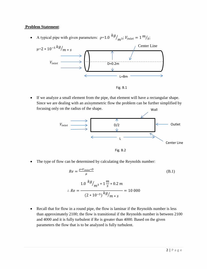
Problem Statement:

A typical pipe with given parameters: ρ=

⁄ ; ⁄ ;

μ= ⁄

If we analyze a small element from the pipe, that element will have a rectangular shape.

Since we are dealing with an axisymmetric flow the problem can be further simplified by

focusing only on the radius of the shape.

The type of flow can be determined by calculating the Reynolds number:

(B.1)

⁄

⁄

Recall that for flow in a round pipe, the flow is laminar if the Reynolds number is less

than approximately 2100; the flow is transitional if the Reynolds number is between 2100

and 4000 and it is fully turbulent if Re is greater than 4000. Based on the given

parameters the flow that is to be analyzed is fully turbulent.

D=0.2m

L=8m

𝑉𝑖𝑛𝑙𝑒𝑡

L

D/2 𝑉𝑖𝑛𝑙𝑒𝑡

Wall

Outlet

Center Line

Center Line

Fig. B.1

Fig. B.2

3 | P a g e

The flow will be analyzed by using Ansys Fluent, however first the geometry and the

corresponding grid must be built. That will be done in Ansys Workbench. Afterwards the

obtained results will be validated in order to make sure they make sense.

Geometry Creation:

Open ANSYS Workbench and start a new project.

Since the flow is to be analyzed in Fluent, drag the Fluid Flow (Fluent) Analysis System

to the project schematic.

Since we are dealing with a 2d geometry, right click on Geometry and select Properties.

Under Advanced Geometry Options for Analysis Type select 2d.

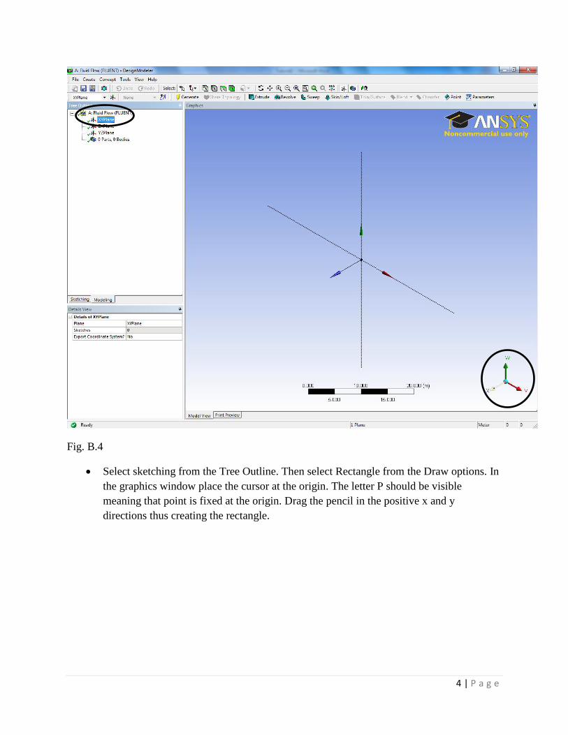
Right click on geometry and select new geometry.

Keep the default units of meters. From the Tree Outline select xy plane, then click the x-

axis in the triad visible in the lower right corner in the graphics window.

Fig. B.3

4 | P a g e

Fig. B.4

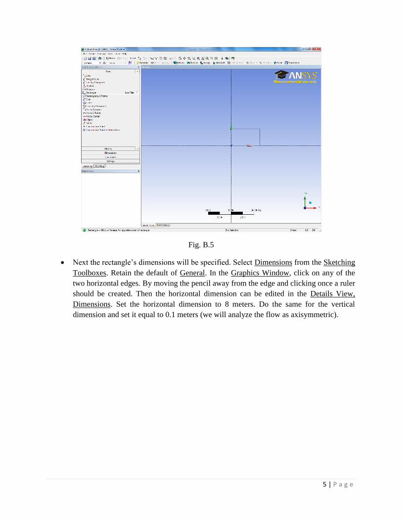
Select sketching from the Tree Outline. Then select Rectangle from the Draw options. In

the graphics window place the cursor at the origin. The letter P should be visible

meaning that point is fixed at the origin. Drag the pencil in the positive x and y

directions thus creating the rectangle.

5 | P a g e

Fig. B.5

Next the rectangle’s dimensions will be specified. Select Dimensions from the Sketching

Toolboxes. Retain the default of General. In the Graphics Window, click on any of the

two horizontal edges. By moving the pencil away from the edge and clicking once a ruler

should be created. Then the horizontal dimension can be edited in the Details View,

Dimensions. Set the horizontal dimension to 8 meters. Do the same for the vertical

dimension and set it equal to 0.1 meters (we will analyze the flow as axisymmetric).

6 | P a g e

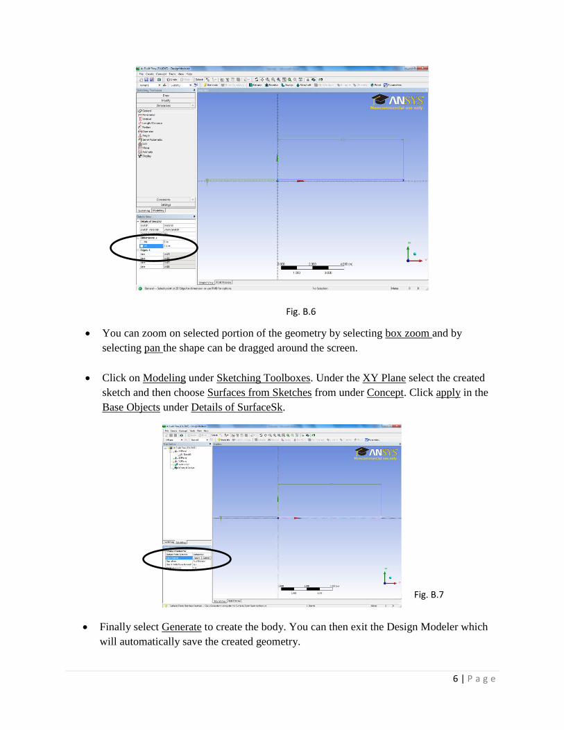
You can zoom on selected portion of the geometry by selecting box zoom and by

selecting pan the shape can be dragged around the screen.

Click on Modeling under Sketching Toolboxes. Under the XY Plane select the created

sketch and then choose Surfaces from Sketches from under Concept. Click apply in the

Base Objects under Details of SurfaceSk.

Finally select Generate to create the body. You can then exit the Design Modeler which

will automatically save the created geometry.

Fig. B.6

Fig. B.7

7 | P a g e

The check mark now visible next to geometry in the project schematic in workbench

indicates no problems are detected and we can proceed with the mesh creation.

Fig. B.8

Mesh Creation:

Double click on Mesh from the Fluid Flow System in the project schematic. Keep the

Meshing Options defaults.

Verify metric units are used (meters, kilograms, Newtons, etc). That can be done by

selecting units.

Select Mesh in the Outline. In Details of Mesh, under Sizing, select Off for Use

Advanced Size Functions. This is necessary since we are manually going to specify the

elements size and mesh type.

Select Mesh Control, then Mapped Face Meshing. Select the face of the body (the

rectangle should turn green) and click apply. By doing so opposite ends will correspond

with each other.

8 | P a g e

Under Mesh Control, select Sizing. Select the edge cube and select both horizontal edges

by holding Ctrl. Click apply.

Fig. B.9

9 | P a g e

Under Type select Number of Divisions. Enter 100 divisions. Next to Behavior choose

Hard. This is to overwrite the sizing function used by the ANSYS mesher. One hundred

divisions are created in the axial direction.

Select both edges.

Fig. B.10

Edge Cube

10 | P a g e

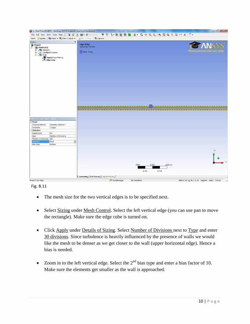
The mesh size for the two vertical edges is to be specified next.

Select Sizing under Mesh Control. Select the left vertical edge (you can use pan to move

the rectangle). Make sure the edge cube is turned on.

Click Apply under Details of Sizing. Select Number of Divisions next to Type and enter

30 divisions. Since turbulence is heavily influenced by the presence of walls we would

like the mesh to be denser as we get closer to the wall (upper horizontal edge). Hence a

bias is needed.

Zoom in to the left vertical edge. Select the 2nd

bias type and enter a bias factor of 10.

Make sure the elements get smaller as the wall is approached.

Fig. B.11

11 | P a g e

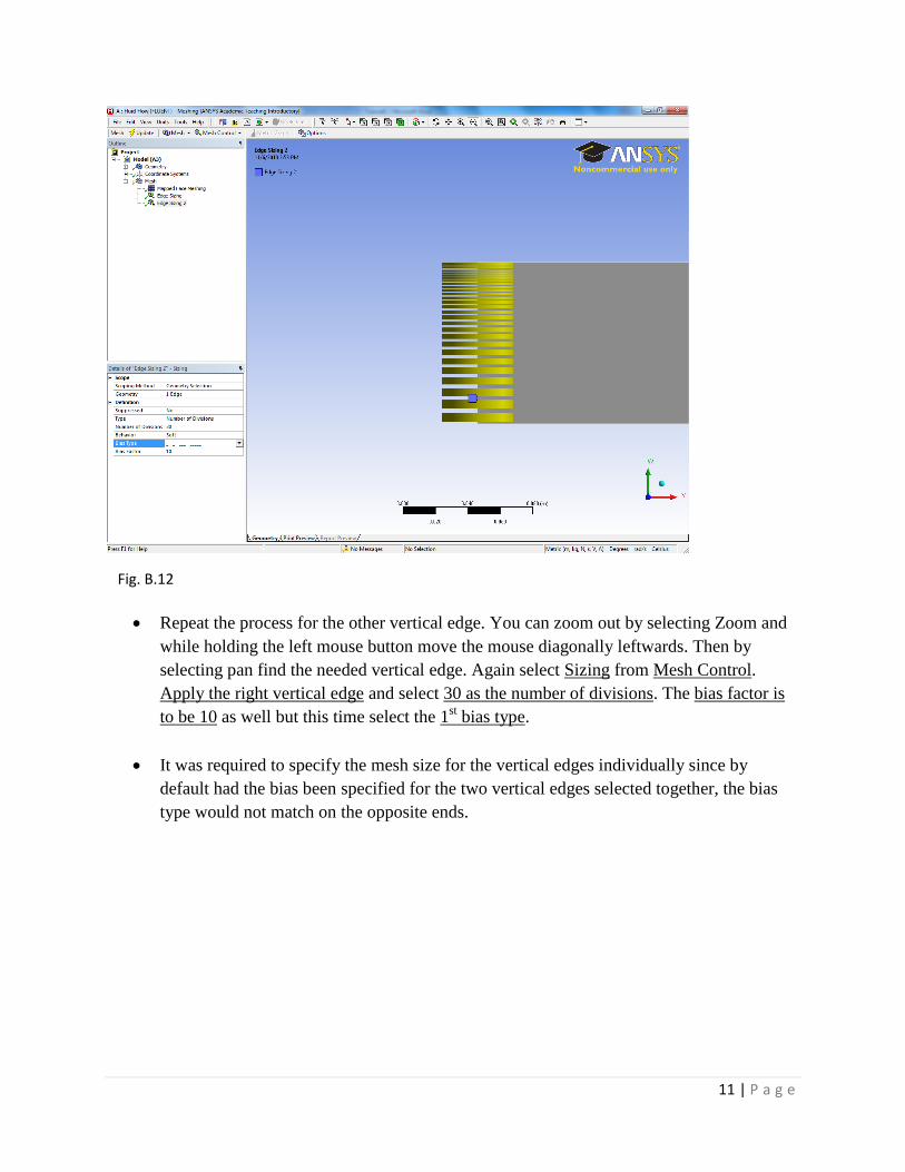
Repeat the process for the other vertical edge. You can zoom out by selecting Zoom and

while holding the left mouse button move the mouse diagonally leftwards. Then by

selecting pan find the needed vertical edge. Again select Sizing from Mesh Control.

Apply the right vertical edge and select 30 as the number of divisions. The bias factor is

to be 10 as well but this time select the 1st bias type.

It was required to specify the mesh size for the vertical edges individually since by

default had the bias been specified for the two vertical edges selected together, the bias

type would not match on the opposite ends.

Fig. B.12

12 | P a g e

The turbulent flow will be analyzed by

using the k-epsilon model which is

primarily valid away from walls

therefore adjustments need to be

made for the model to be accurate

near walls. Hence a bias is required to

provide more mesh near the wall.

Fig. B.13

13 | P a g e

Next the zones are to be named. Select the upper horizontal edge. Right click and select

Create Named Selections. Type Wall. Similarly type Inlet for the left vertical edge, Outlet

for the right one, and Center Line for the bottom horizontal edge. It is necessary to

specify the zones since the boundary conditions will be applied for those named zones in

Fluent.

Fig.B.14

Finally click on Update. The mesh should look like depicted in Fig. B.15.

Fig. B.15 depicts a structured (mesh consisting of rectangles exhibiting a pronounced

pattern) mesh of size 100X30--thirty divisions in the radial direction and 100 divisions in

the axial one. You can now exit Meshing (it will be automatically saved).

In the project schematic, next to meshing a check mark should appear signaling no issues

were found. Double click on Setup.

14 | P a g e

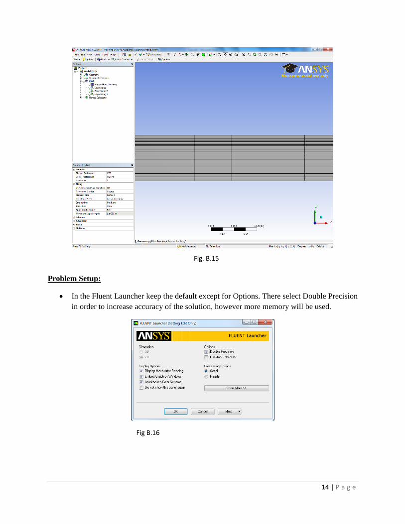
Problem Setup:

In the Fluent Launcher keep the default except for Options. There select Double Precision

in order to increase accuracy of the solution, however more memory will be used.

Fig. B.15

Fig B.16

15 | P a g e

Once in Fluent, in Problem Setup—General, select check. The mesh will be checked by

Fluent and any errors will be reported. In Volume Statistics make sure the minimum

volume is positive since if it is not, computation will not be possible.

In General—Solver, keep the defaults except for 2D space. There choose axisymmetric.

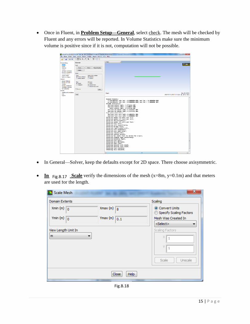
In General-- Scale verify the dimensions of the mesh (x=8m, y=0.1m) and that meters

are used for the length.

Fig.B.17

Fig.B.18

16 | P a g e

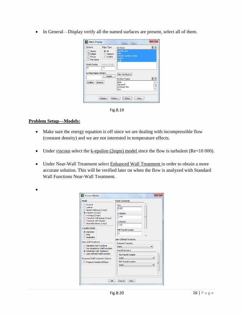
In General—Display verify all the named surfaces are present, select all of them.

Problem Setup—Models:

Make sure the energy equation is off since we are dealing with incompressible flow

(constant density) and we are not interested in temperature effects.

Under viscous select the k-epsilon (2eqns) model since the flow is turbulent (Re=10 000).

Under Near-Wall Treatment select Enhanced Wall Treatment in order to obtain a more

accurate solution. This will be verified later on when the flow is analyzed with Standard

Wall Functions Near-Wall Treatment.

Fig.B.19

Fig.B.20

17 | P a g e

Problem Setup—Materials:

Double click on air. Enter

⁄ for the density and ⁄ for the

viscosity. Enter change/create—the entered data overwrites the pre-existing material

information.

If the material is saved not overwriting the pre-existing air material but is saved as a

separate material (ex. the data is saved as material named ‘custom’) an extra step is

required to make sure the model is analyzed using the proper material properties.

In Problem Setup—Cell Zone Conditions, double click the surface_body zone. Under

Material Name make sure the proper material is selected—in the given example the

material named ‘custom’ should be selected. Press OK.

Fig.B.21

18 | P a g e

Problem Setup—Boundary Conditions:

Verify and if needed change the zone types as depicted in Table B.1

Zone Type

center_line Axis

inlet Velocity-inlet

Interior-surface body Interior

outlet Pressure-outlet

wall Wall

Double Click on inlet. Enter 1m/s for the velocity magnitude (given value). Under

Turbulence, select Intensity and Hydraulic Diameter.

Specify 1% for Turbulent Intensity and 0.2meters for the Hydraulic Diameter.

Table B.1

Fig B.22

19 | P a g e

Problem Setup—Boundary Conditions:

Double click on outlet. Verify the gauge pressure is set to 0 (since the difference between

the absolute pressure at the outlet, 1atm, and the operating pressure, 1 atm, equals to 0

which is the gauge pressure at the outlet).

Fig.B.24

Verify in the Operating Conditions that the Operating Pressure is set to 101, 325 Pa

which equals 1 atm.

Fig B.23

20 | P a g e

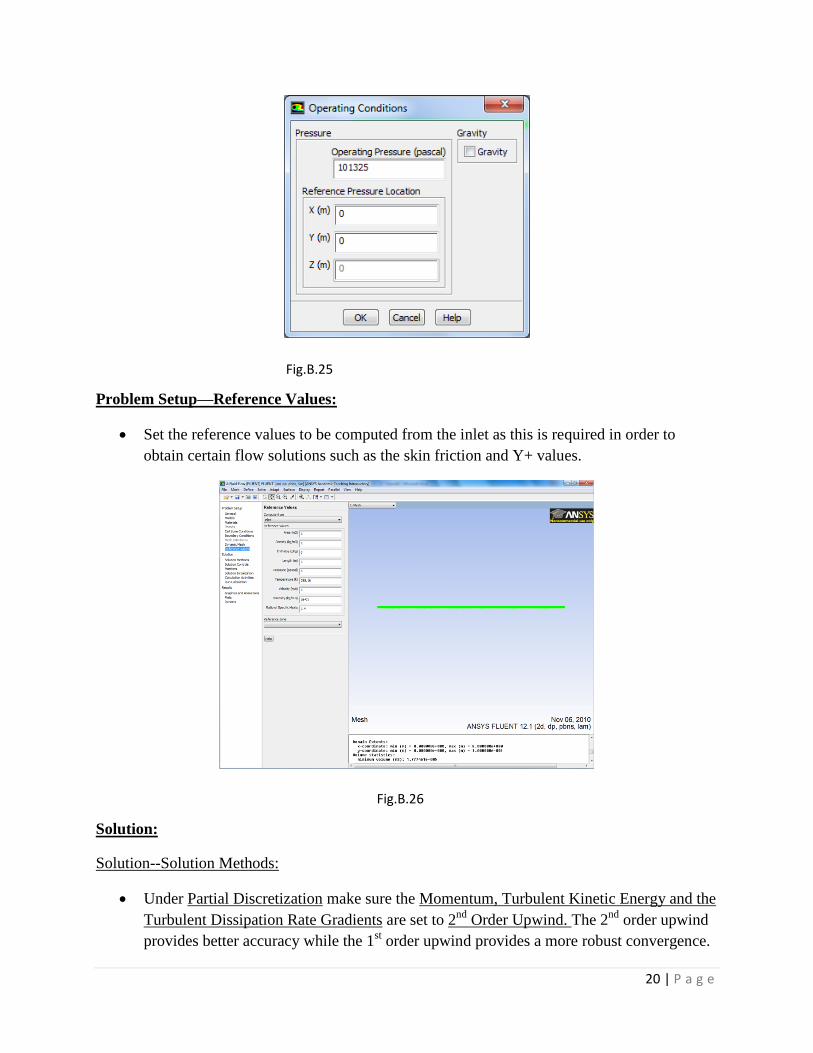
Problem Setup—Reference Values:

Set the reference values to be computed from the inlet as this is required in order to

obtain certain flow solutions such as the skin friction and Y+ values.

Solution:

Solution--Solution Methods:

Under Partial Discretization make sure the Momentum, Turbulent Kinetic Energy and the

Turbulent Dissipation Rate Gradients are set to 2nd

Order Upwind. The 2nd

order upwind

provides better accuracy while the 1st order upwind provides a more robust convergence.

Fig.B.25

Fig.B.26

21 | P a g e

Fig.B.27

Solution—Monitors:

Double click on Residuals. Make sure the Print to Console and Plot options are checked.

In Equations set the absolute criteria to 1e-06 for all 5 equations. Residuals provide a

measure of how well the current solution satisfies the discrete form of each of the

governing equations.

Fig.B.28

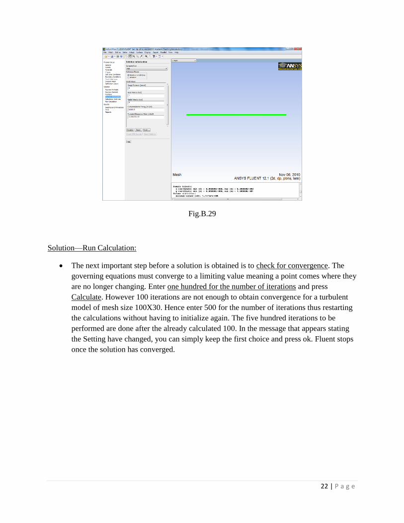
Solution—Initialization:

The input data and conditions must be initialized in order for a solution to be obtained.

Select Compute from Inlet and press Initialize.

22 | P a g e

Fig.B.29

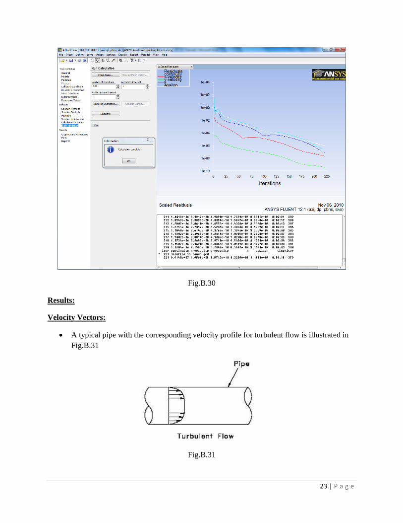
Solution—Run Calculation:

The next important step before a solution is obtained is to check for convergence. The

governing equations must converge to a limiting value meaning a point comes where they

are no longer changing. Enter one hundred for the number of iterations and press

Calculate. However 100 iterations are not enough to obtain convergence for a turbulent

model of mesh size 100X30. Hence enter 500 for the number of iterations thus restarting

the calculations without having to initialize again. The five hundred iterations to be

performed are done after the already calculated 100. In the message that appears stating

the Setting have changed, you can simply keep the first choice and press ok. Fluent stops

once the solution has converged.

23 | P a g e

Fig.B.30

Results:

Velocity Vectors:

A typical pipe with the corresponding velocity profile for turbulent flow is illustrated in

Fig.B.31

Fig.B.31

24 | P a g e

The velocity profile can be displayed by going to Results—Graphics and Animations and

double clicking Vectors under Graphics—Fig.B.32. Refer to Appendix A—Results about

colormap and vectors manipulation. Fig.B.33 showcases the fully developed velocity

vectors.

Fig.B.32

Fig.B.33—Fully Developed Velocity Vectors near the Pipe’s Outlet

Axis

Outlet

25 | P a g e

XY Plots will be performed for the Y+values, centerline velocity in the axial direction,

the skin friction coefficient, the fully developed velocity profile in the radial direction and

the pressure drop. The solutions will then be validated against the theoretical data in

order to make sure they are correct and make sense. Finally by improving the mesh we

will try to obtain a more accurate solution.

Y+values:

o In Results—Plots select XY Plot. Double click it. Make sure Position on X axis is

selected as well as Node Values. In Plot Direction make sure x=1 and y=0 (x will

thus become the abscissa or horizontal coordinate). Select Turbulence from under

Y Axis Function and choose Wall Yplus. Select the wall surface. Click on Plot.

Fig.B.34

Fig.B.35

Y+ is a non-dimensional wall distance

for a wall-bounded flow. It is given as

𝒚+ 𝒖 𝒚

𝝂 (B.2)

where y is the distance to the nearest

wall 𝑢 is the friction velocity at the

nearest wall, 𝜈 is the local kinematic

viscosity.

Y+ is calculated from the reference

values specified—ρ, µ, 𝑉𝑖𝑛𝑙𝑒𝑡

26 | P a g e

The graph can be saved as a picture by selecting Save Picture under File. The different

saving options are explained when Help is pressed.

The graph can be manipulated –by going back to the XY Plot and selecting curves, the

markers can be replaced by a line with a user chosen color and weight.

Fig.B.36

The graph can be further enhanced by manipulating the y-axis values. By selecting Axes,

in the number format the type can be changed from exponential to float. Make sure to

click apply after a change has been made for a particular axis. The graph produced as a

result is shown in Graph.B.1:

Graph.B.1

27 | P a g e

Fig.B.37

Fig.B.38

Results—Centerline Velocity PlotIn Results—Plots, XY Plot, in the Y-axis function select

Velocity and Axial Velocity. Deselect the wall surface by clicking it again and select the

centerline surface. Click Plot

The plot can be saved by clicking on Write to

File in the Solution XY Plot window. Press

Write afterwards and save the plot as a .xy file.

The .xy file can be then opened in Excel where

dimensional analysis for validation purposes

can be performed. This will be demonstrated

later.

28 | P a g e

.

Graph.B.2

Fig.B.39

The title of the plot can be changed by double clicking on the default text in the lower left

corner. Save the plot by selecting the Write to File and clicking Write.

It can be seen the fully developed region starts at around x=4m.

Results—Skin Friction Coefficient:

In the XY Plot window select Wall Fluxes under Y-axis Function and specify Skin

Friction Coefficient. Select the Wall Surface.

29 | P a g e

Graph.B.3

Fig.B.40

Skin friction, is the drag on the plate produced by the boundary layer due to viscous

stresses which are developed at the wall. It also reffered as the Fanning friction factor.

(B.3)

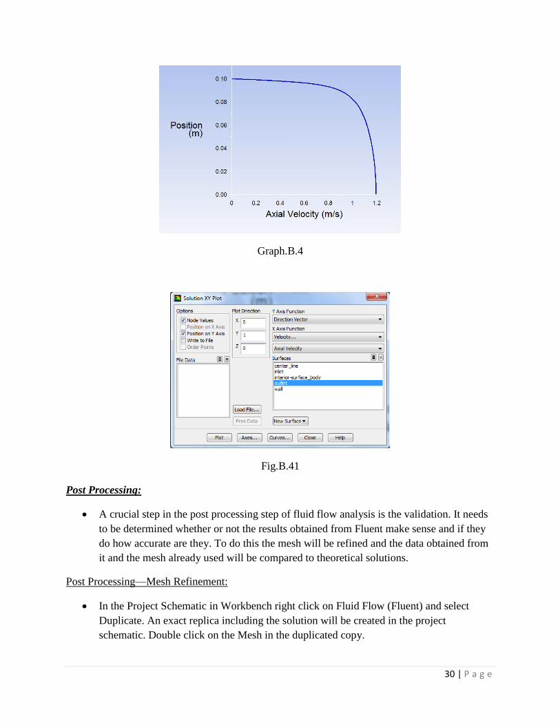
Results— FD Velocity Profile:

In the Solution XY Plot deselect Position on X Axis and select Position on Y axis since

we are to plot the velocity profile in the radial direction. In Plot Direction set x=0 and

y=1. Under X Axis Function select Velocity and specify Axial Velocity. Since we are

interested in the fully developed profile select the outlet surface. Save the created plot.

30 | P a g e

Graph.B.4

Fig.B.41

Post Processing:

A crucial step in the post processing step of fluid flow analysis is the validation. It needs

to be determined whether or not the results obtained from Fluent make sense and if they

do how accurate are they. To do this the mesh will be refined and the data obtained from

it and the mesh already used will be compared to theoretical solutions.

Post Processing—Mesh Refinement:

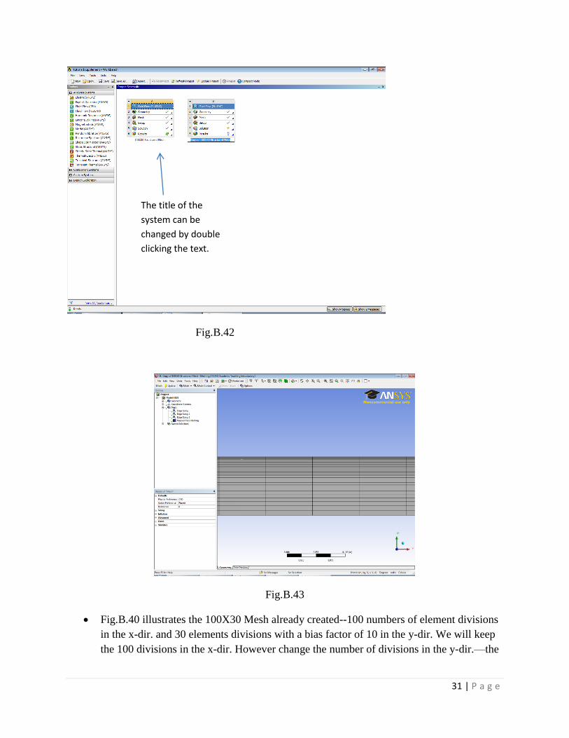
In the Project Schematic in Workbench right click on Fluid Flow (Fluent) and select

Duplicate. An exact replica including the solution will be created in the project

schematic. Double click on the Mesh in the duplicated copy.

31 | P a g e

Fig.B.42

Fig.B.43

Fig.B.40 illustrates the 100X30 Mesh already created--100 numbers of element divisions

in the x-dir. and 30 elements divisions with a bias factor of 10 in the y-dir. We will keep

the 100 divisions in the x-dir. However change the number of divisions in the y-dir.—the

The title of the

system can be

changed by double

clicking the text.

32 | P a g e

2 vertical edges with the bias factor of 10 from 30 to 60 divisions. Click Update when

finished.

Fig.B.44

The Mapped Face Meshing failed (the check mark next its name was replaced) because it

became over constrained. There are two way to fix the problem—reduce the bias factor

or decrease the number of divisions.

Fig.B.45

Fig.B.42 showcases the refined structured 100X60 Mesh upon changing the bias factor

for the 2 vertical edges from 10 to 8.

33 | P a g e

Fig.B.46

Fig.B.43 illustrates the refined structured 100X54 Mesh with a bias factor for the vertical

edges of 10. If the number of divisions is increased more than 54 the mesh becomes over

constrained. This is the mesh we will use for the post processing analysis.

After exiting the mesh builder a check mark should appear next to Mesh in the Project

Schematic indicating no issues are found in the mesh and it can be used in Fluent for

analysis. Double click on Setup and if a message appears stating the upstream mesh has

been changed press yes in order to load the new mesh in Fluent. Go through the setup

process performed for the 100X30 mesh in order to verify nothing has been changed

upon duplicating the system in Workbench.

Make sure the reference values are set to be computed from the inlet as well as initialize

the solution from the inlet. The solution converged at the 221 iteration for the 100X30

Mesh however since the mesh was refined convergence now is achieved at the 564

iteration:

34 | P a g e

Graph.B.5

Obtain the same XY Plots in the same manner as with the 100X30 Mesh. Make sure to

save the files so we can perform dimensional analysis.

More than one curve can be plotted in a graph. Let us now plot the Y+values for the

100X54 mesh as well as those for the 100X30 mesh both in Fluent. The XY plot for the

Y+values for the 100X54 is done just like we did before: Results—Plots—XY Plot, Y

axis function set as turbulence and specified as wall y plus at the wall surface. Select

Load File and find the location where the Y+ XY Plot for the 100X30 Mesh was saved.

Click Plot.

35 | P a g e

Graph.B.6

Fig.B.47

The red curve in Graph.B.6 corresponds to the 100X54 Mesh and the blue one—to the

100X30 one.

All the data obtained so far is done with the help of the k-epsilon method with enhanced

wall treatment. What if a difference k-epsilon method is used? Would the data be more

accurate then?

Let us duplicate in Workbench the 100X54 Fluid Flow system. The geometry and mesh

need not be changed. Double click on setup to start up Fluent. In Problem Setup, Models,

double click Viscous. In the Near Wall Treatment box the Enhanced Wall Treatment

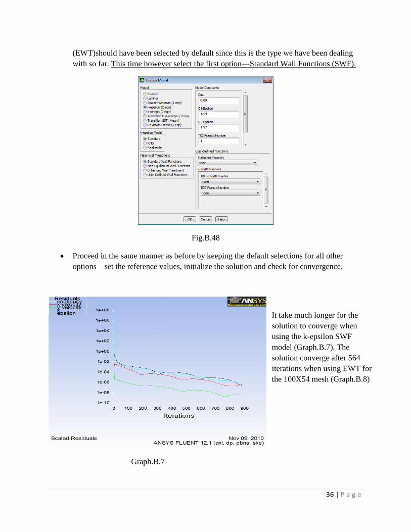
36 | P a g e

(EWT)should have been selected by default since this is the type we have been dealing

with so far. This time however select the first option—Standard Wall Functions (SWF).

Fig.B.48

Proceed in the same manner as before by keeping the default selections for all other

options—set the reference values, initialize the solution and check for convergence.

Graph.B.7

It take much longer for the

solution to converge when

using the k-epsilon SWF

model (Graph.B.7). The

solution converge after 564

iterations when using EWT for

the 100X54 mesh (Graph.B.8)

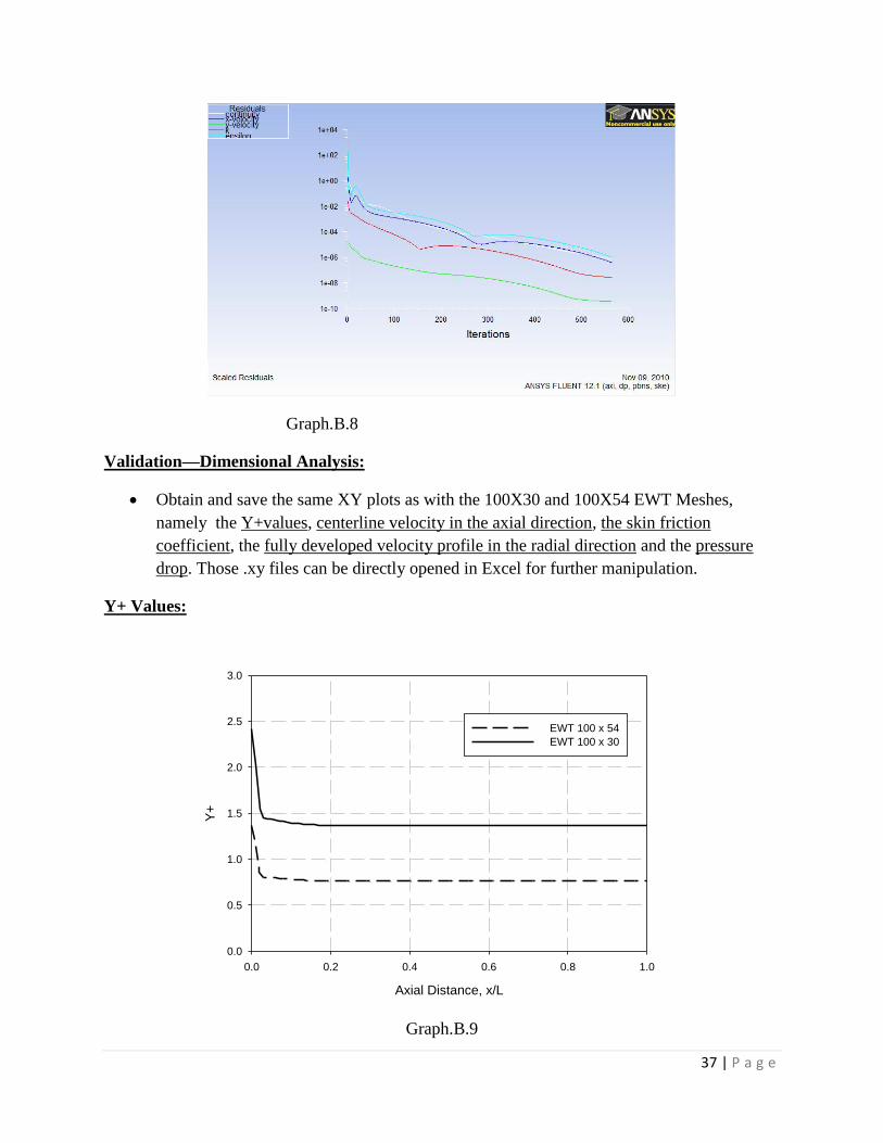
37 | P a g e

Graph.B.8

Validation—Dimensional Analysis:

Obtain and save the same XY plots as with the 100X30 and 100X54 EWT Meshes,

namely the Y+values, centerline velocity in the axial direction, the skin friction

coefficient, the fully developed velocity profile in the radial direction and the pressure

drop. Those .xy files can be directly opened in Excel for further manipulation.

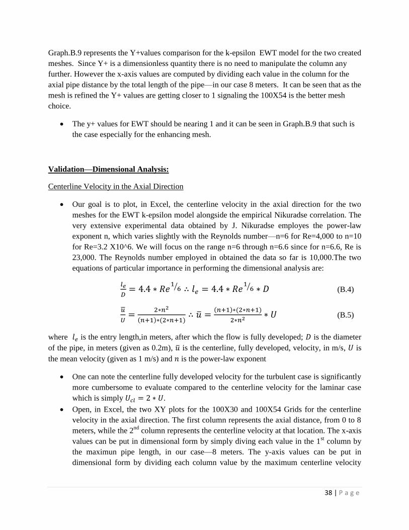
Y+ Values:

Axial Distance, x/L

0.0 0.2 0.4 0.6 0.8 1.0

Y+

0.0

0.5

1.0

1.5

2.0

2.5

3.0

EWT 100 x 54

EWT 100 x 30

Graph.B.9

38 | P a g e

Graph.B.9 represents the Y+values comparison for the k-epsilon EWT model for the two created

meshes. Since Y+ is a dimensionless quantity there is no need to manipulate the column any

further. However the x-axis values are computed by dividing each value in the column for the

axial pipe distance by the total length of the pipe—in our case 8 meters. It can be seen that as the

mesh is refined the Y+ values are getting closer to 1 signaling the 100X54 is the better mesh

choice.

The y+ values for EWT should be nearing 1 and it can be seen in Graph.B.9 that such is

the case especially for the enhancing mesh.

Validation—Dimensional Analysis:

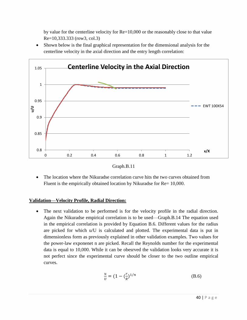
Centerline Velocity in the Axial Direction

Our goal is to plot, in Excel, the centerline velocity in the axial direction for the two

meshes for the EWT k-epsilon model alongside the empirical Nikuradse correlation. The

very extensive experimental data obtained by J. Nikuradse employes the power-law

exponent n, which varies slightly with the Reynolds number—n=6 for Re=4,000 to n=10

for Re=3.2 X10^6. We will focus on the range n=6 through n=6.6 since for n=6.6, Re is

23,000. The Reynolds number employed in obtained the data so far is 10,000.The two

equations of particular importance in performing the dimensional analysis are:

⁄

⁄ (B.4)

(B.5)

where is the entry length,in meters, after which the flow is fully developed; is the diameter

of the pipe, in meters (given as 0.2m), is the centerline, fully developed, velocity, in m/s, is

the mean velocity (given as 1 m/s) and is the power-law exponent

One can note the centerline fully developed velocity for the turbulent case is significantly

more cumbersome to evaluate compared to the centerline velocity for the laminar case

which is simply .

Open, in Excel, the two XY plots for the 100X30 and 100X54 Grids for the centerline

velocity in the axial direction. The first column represents the axial distance, from 0 to 8

meters, while the 2nd

column represents the centerline velocity at that location. The x-axis

values can be put in dimensional form by simply diving each value in the 1st column by

the maximun pipe length, in our case—8 meters. The y-axis values can be put in

dimensional form by dividing each column value by the maximum centerline velocity

39 | P a g e

value for the corresponding grid. The graphical representation is shown below (note the

y-axis is readjusted in order to improve visualization):

Axial Distance, x/L

0.0 0.2 0.4 0.6 0.8 1.0

Ce

nte

rlin

e V

elo

city, u

/U

0.85

0.90

0.95

1.00

1.05

Fluent 100 x 30

Fluent 100 x 54

Graph.B.10

Note that refining the mesh while having a significant impact on the Y+values, does not

produce any noticeable change in the centerline velocity profile. Also fully developed

flow starts at around 0.5 of the pipe’s length.

The next step is to plot the Nikuradse empirical correlation for n=6 through n=6.6

Since we are going to focus on n=6 through n=6.6 and we know the Reynolds number at

those two locations we can assume a linear relationship with a reasonable degree of

accuracy for that small interval. Hence the Reynolds values are divided equally for than n

interval and column 3 is obtained.

The first column contains the theoretical entry length distance obtained by eq. 1) for the

particular Re for that row. Column 2 is the dimensionless form of the entry length

distance—each entry length value is divided by the total pipe length which is 8 meters.

Column 4 is the range of power-law exponents while column 5 is the given mean or

average velocity of 1 m/s.

The fifth column is the centerline fully developed velocity obtained by using eq. (2) for

the particular n value.

The last column is the dimensionless form of the F.D. centerline velocity. Since we are

concerned with the Re for our flow which is 10, 000 each value for the velocity is divided

40 | P a g e

by value for the centerline velocity for Re=10,000 or the reasonably close to that value

Re=10,333.333 (row3, col.3)

Shown below is the final graphical representation for the dimensional analysis for the

centerline velocity in the axial direction and the entry length correlation:

Graph.B.11

The location where the Nikuradse correlation curve hits the two curves obtained from

Fluent is the empirically obtained location by Nikuradse for Re= 10,000.

Validation—Velocity Profile, Radial Direction:

The next validation to be performed is for the velocity profile in the radial direction.

Again the Nikuradse empirical correlation is to be used—Graph.B.14 The equation used

in the empirical correlation is provided by Equation B.6. Different values for the radius

are picked for which u/U is calculated and plotted. The experimental data is put in

dimensionless form as previously explained in other validation examples. Two values for

the power-law exponenet n are picked. Recall the Reynolds number for the experimental

data is equal to 10,000. While it can be obesrved the validation looks very accurate it is

not perfect since the experimental curve should be closer to the two outline empirical

curves.

⁄ (B.6)

0.8

0.85

0.9

0.95

1

1.05

0 0.2 0.4 0.6 0.8 1 1.2

u/U

x/X

Centerline Velocity in the Axial Direction

EWT 100X54

41 | P a g e

Axial Velocity, u/ucl

0.0 0.2 0.4 0.6 0.8 1.0

Ra

dia

l D

ista

nce

, r/

R

0.0

0.2

0.4

0.6

0.8

1.0

EWT 100 x 54

EWT 100 x 30

Nikuradse, n=6

Nikuradse, n=7

Graph.B.12

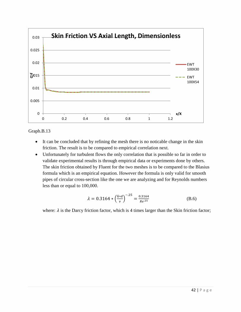
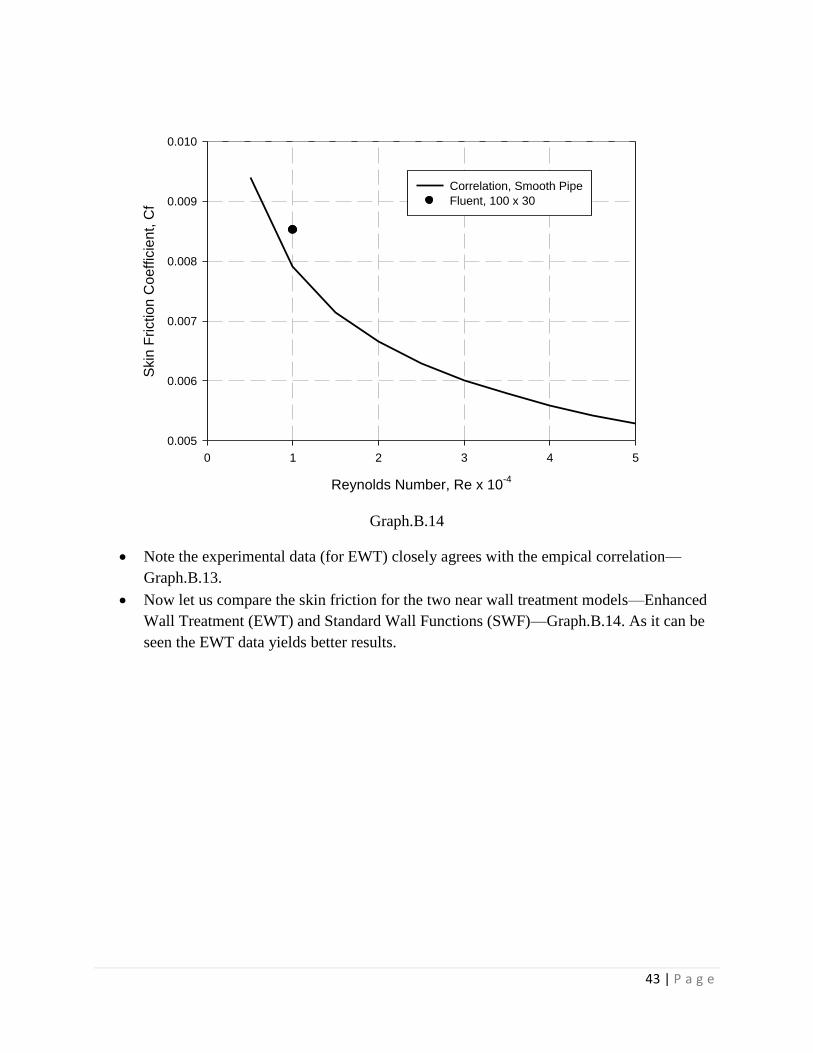
Validation—Skin Friction:

The skin friction coefficients for the EWT model can be compared for the two created

meshes. Open the two previosly saved .xy plots for the skin friction in the axial distance

and dimensionalize the x-axis by simply dividing every single axial value by the total

distance of the pipe. There is no need to dimensionalize the skin friction coefficient since

it is already dimensionless. The resulting graph can be seen below:

42 | P a g e

Graph.B.13

It can be concluded that by refining the mesh there is no noticable change in the skin

friction. The result is to be compared to empirical correlation next.

Unfortunately for turbulent flows the only correlation that is possible so far in order to

validate experimental results is through empirical data or experiments done by others.

The skin friction obtained by Fluent for the two meshes is to be compared to the Blasius

formula which is an empirical equation. However the formula is only valid for smooth

pipes of circular cross-section like the one we are analyzing and for Reynolds numbers

less than or equal to 100,000.

(

)

(B.6)

where: is the Darcy friction factor, which is 4 times larger than the Skin friction factor;

0

0.005

0.01

0.015

0.02

0.025

0.03

0 0.2 0.4 0.6 0.8 1 1.2

C_f

x/X

Skin Friction VS Axial Length, Dimensionless

EWT100X30

EWT100X54

43 | P a g e

Reynolds Number, Re x 10-4

0 1 2 3 4 5

Skin

Friction C

oeffic

ient, C

f

0.005

0.006

0.007

0.008

0.009

0.010

Correlation, Smooth Pipe

Fluent, 100 x 30

Graph.B.14

Note the experimental data (for EWT) closely agrees with the empical correlation—

Graph.B.13.

Now let us compare the skin friction for the two near wall treatment models—Enhanced

Wall Treatment (EWT) and Standard Wall Functions (SWF)—Graph.B.14. As it can be

seen the EWT data yields better results.

44 | P a g e

Axial Distance, x/L

0.0 0.1 0.2 0.3 0.4 0.5 0.6

Skin

Frictio

n C

oe

ffic

ien

t, C

f

0.000

0.005

0.010

0.015

0.020

0.025

0.030

SWT, 100 x 54

SWT, 100 x 30

EWT, 100 x 54

EWT, 100 x 30

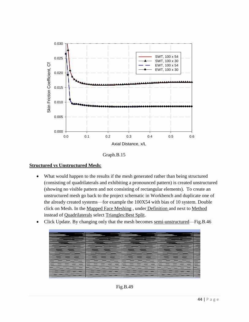
Graph.B.15

Structured vs Unstructured Mesh:

What would happen to the results if the mesh generated rather than being structured

(consisting of quadrilaterals and exhibiting a pronounced pattern) is created unstructured

(showing no visible pattern and not consisting of rectangular elements). To create an

unstructured mesh go back to the project schematic in Workbench and duplicate one of

the already created systems—for example the 100X54 with bias of 10 system. Double

click on Mesh. In the Mapped Face Meshing , under Definition and next to Method

instead of Quadrilaterals select Triangles:Best Split.

Click Update. By changing only that the mesh becomes semi-unstructured—Fig.B.46

Fig.B.49

45 | P a g e

You can verify in Ansys that unfortunately if this mesh is used the solution does not

converge and an accurate result cannot be obtained. If you go back in Workbench we can

modify this mesh even further by selecting a bias not only for the vertical edges but for

the horizontal ones as well. Do the bias for two edges at a time (the two horizontal ones

and the two vertical ones). Select a bias of 7 for the horizontal edges –Fig.B.47.

Fig.B.50

Graph.B.16

As it can be seen the solution does not converge (Graph.B.15) meaning erroneous results

will be obtained as it can be seen in the XY Plot generated in Ansys for the centerline

velocity profile in the axial direction—Graph.B.16. Compare the velocity profile for the

unstructured mesh (blue curve) with the profile for the structured one (red curve)—

Graph.B.17.Hence it is important when generating the mesh to make sure it is a

structured one.

46 | P a g e

Graph.B.17

Graph.B.18