tsunami modeling - governing equations - linear form of shallow water equations in spherical...
TRANSCRIPT

TSUNAMI MODELING

- Governing Equations
- Linear form of Shallow Water Equations in Spherical Coordinates for Far Field Tsunami Modeling
- TWO-LAYER Numerical Model for Tsunami Generation and Wave Propagation
- Comparison of Analytical and Numerical Approaches for Long Wave Runup
Content
Tsunami’s approach to the shore Summary

Context
Two scenarios need consideration:
Locally generated tsunamisFor this case warning commonly comesfrom perceiving earthquake motionunless caused by landslide.Timescale for warning – a few minutes.
Tsunamis arriving after significant propagationUsually approaching from deep water.Maybe an hour or more available for warning.
For both cases there is need for consideration of flows at various scales, including:
oceanic, regional, coastal features, and local structures,i.e. “nested” models
for assessment of vulnerable areas.
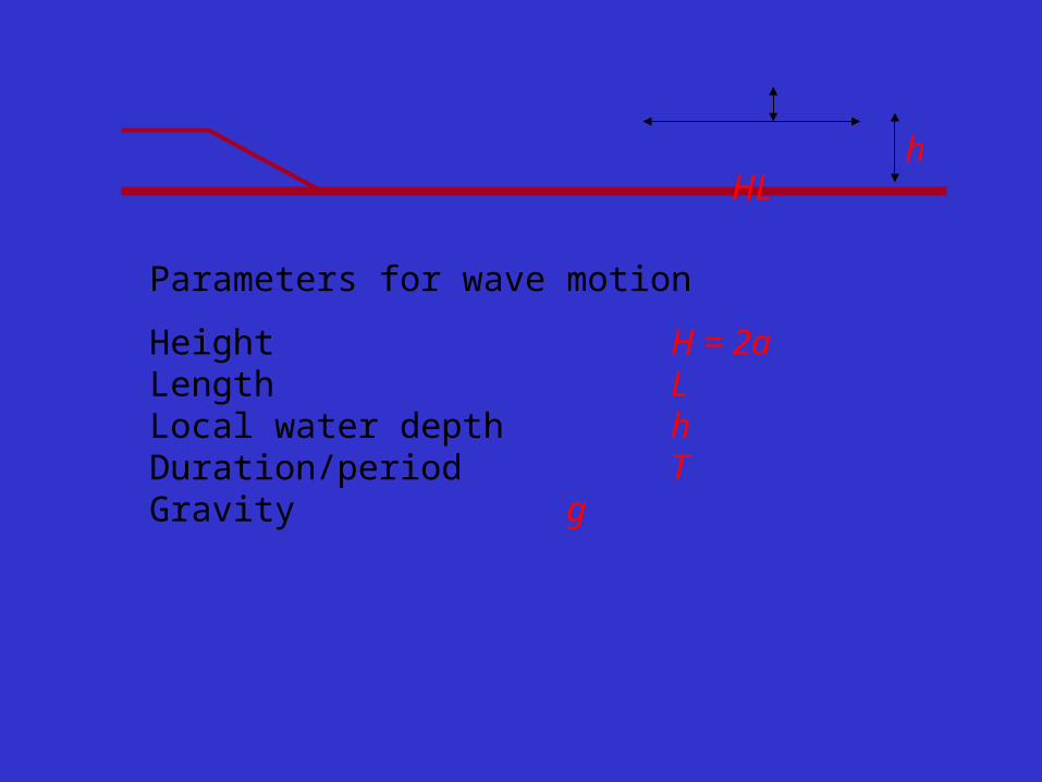
Parameters for wave motion
Height H = 2aLength L Local water depth h Duration/period TGravity g
HL
h

a L
h
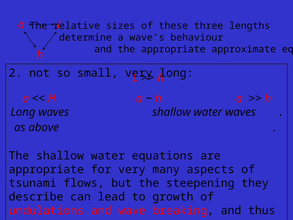
The relative sizes of these three lengths determine a wave’s behaviour and the appropriate approximate equations.
a << h a << L
Linear waves
L >> h L ~ h L << hLong waves intermediate depth deep water waves
non-dispersive dispersive
generally appropriate for the deep ocean
1. Very small, very slight slopes
a L
h
The relative sizes of these three lengths determine a wave’s behaviour and the appropriate approximate equations.
L >> h
a << H a ~ h a >> hLong waves shallow water waves .as above wave front steepening .
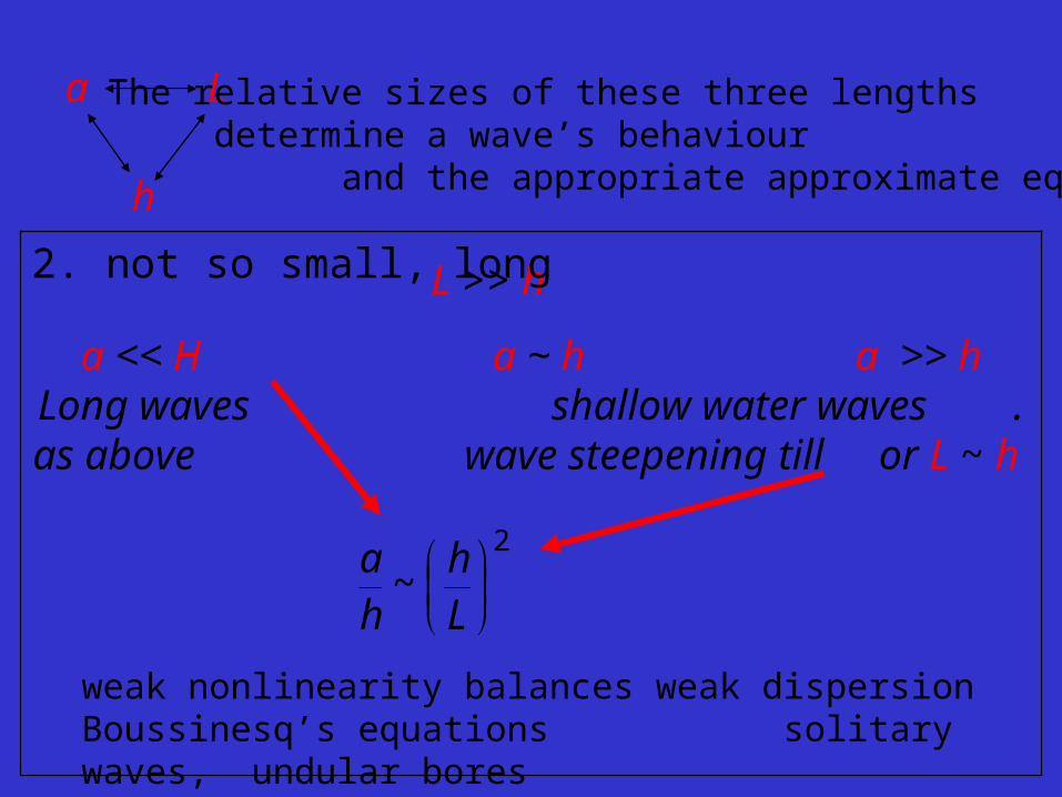
2. not so small, very long:
The shallow water equations are appropriate for very many aspects of tsunami flows, but the steepening they describe can lead to growth of undulations and wave breaking, and thus failure of the approximation.
a L
h
The relative sizes of these three lengths determine a wave’s behaviour and the appropriate approximate equations.
L >> h
a << H a ~ h a >> hLong waves shallow water waves .as above wave steepening till or L ~ h
2. not so small, long
2
~
Lh
ha
weak nonlinearity balances weak dispersionBoussinesq’s equations solitary waves, undular bores
a L
h
The relative sizes of these three lengths determine a wave’s behaviour and the appropriate approximate equations.
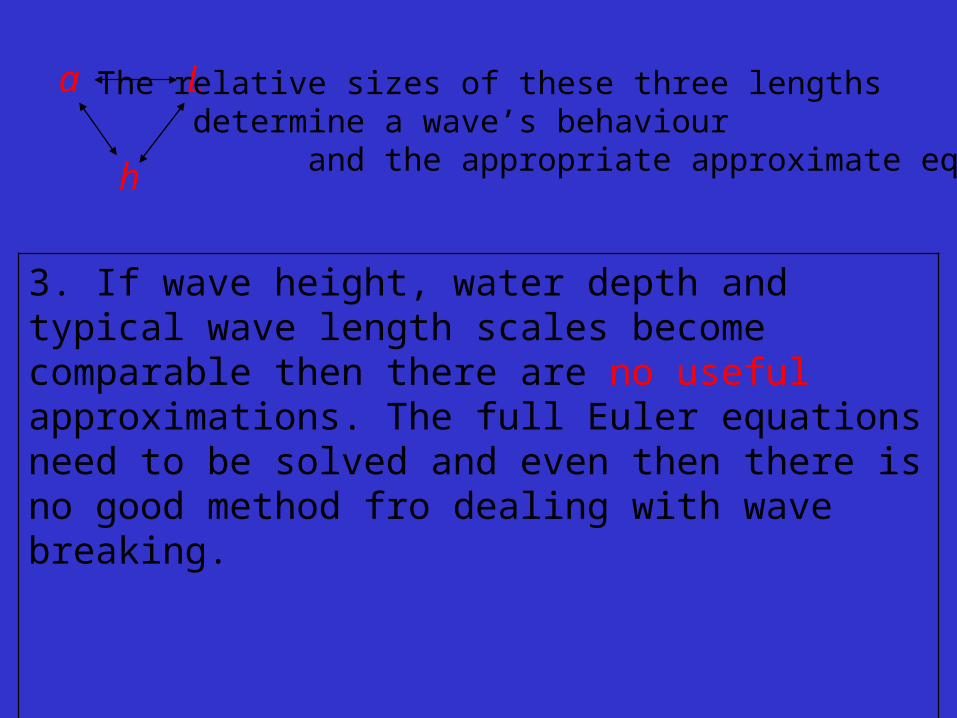
3. If wave height, water depth and typical wave length scales become comparable then there are no useful approximations. The full Euler equations need to be solved and even then there is no good method fro dealing with wave breaking.
In such cases one usually has to make do with the approximation of bores modelled as discontinuities within the shallow water equations.
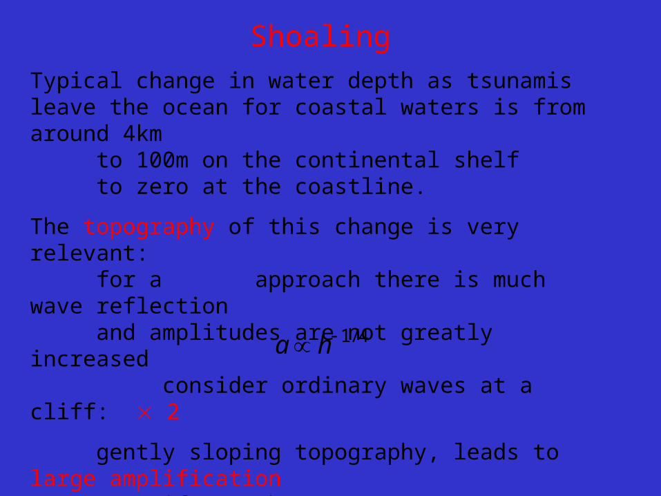
Shoaling
Typical change in water depth as tsunamis leave the ocean for coastal waters is from around 4km
to 100m on the continental shelf to zero at the coastline.
The topography of this change is very relevant:for a steep approach there is much wave reflection and amplitudes are not greatly increased
consider ordinary waves at a cliff: 2
gently sloping topography, leads to large amplificationif 2D, then until a ~ h 4/1 ha
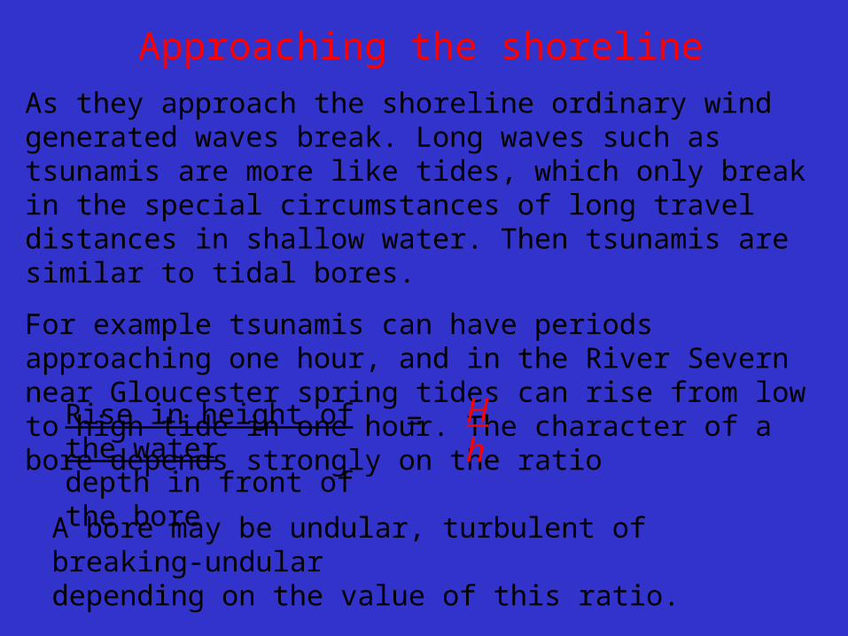
Approaching the shoreline
As they approach the shoreline ordinary wind generated waves break. Long waves such as tsunamis are more like tides, which only break in the special circumstances of long travel distances in shallow water. Then tsunamis are similar to tidal bores.
For example tsunamis can have periods approaching one hour, and in the River Severn near Gloucester spring tides can rise from low to high tide in one hour. The character of a bore depends strongly on the ratio
Rise in height of the waterdepth in front of the bore
= Hh
A bore may be undular, turbulent of breaking-undulardepending on the value of this ratio.
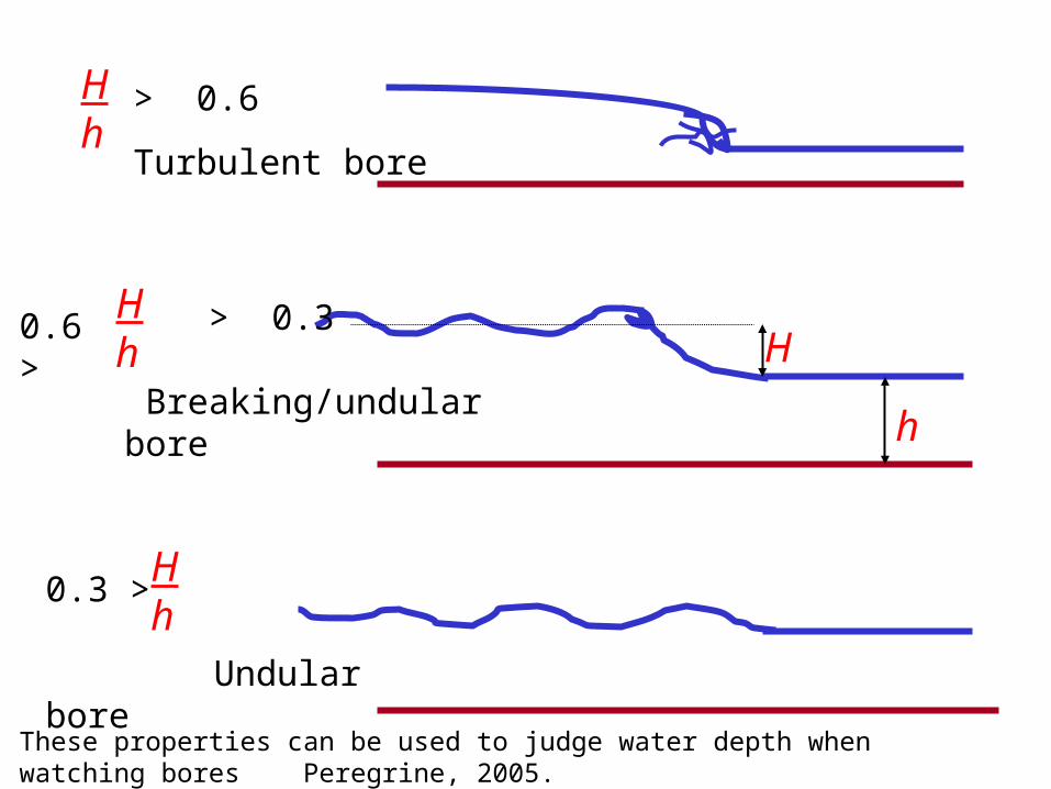
Hh
> 0.6
Turbulent bore
Hh
0.6 > > 0.3
Breaking/undular bore
Hh
0.3 >
Undular bore
h
H
These properties can be used to judge water depth when watching bores Peregrine, 2005.
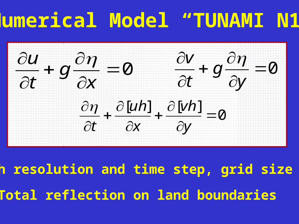
Numerical Model “TUNAMI N1”
0
xg
t
u 0
yg
t
v
0][][
y
vh
x
uh
t
Mesh resolution and time step, grid size
Total reflection on land boundaries
Governing Equations
0
y +hv
x+hu
t
0 x
y
u v
x
u
t
u
xgu
0y
y
vv
x
v
t
v
ygu
η : water elevationu, v : components of water velocities in x and y directionsy : bottom shear stress components ح ,xحt : timeh : basin depthg : gravitational acceleration
Non-linear longwave equations
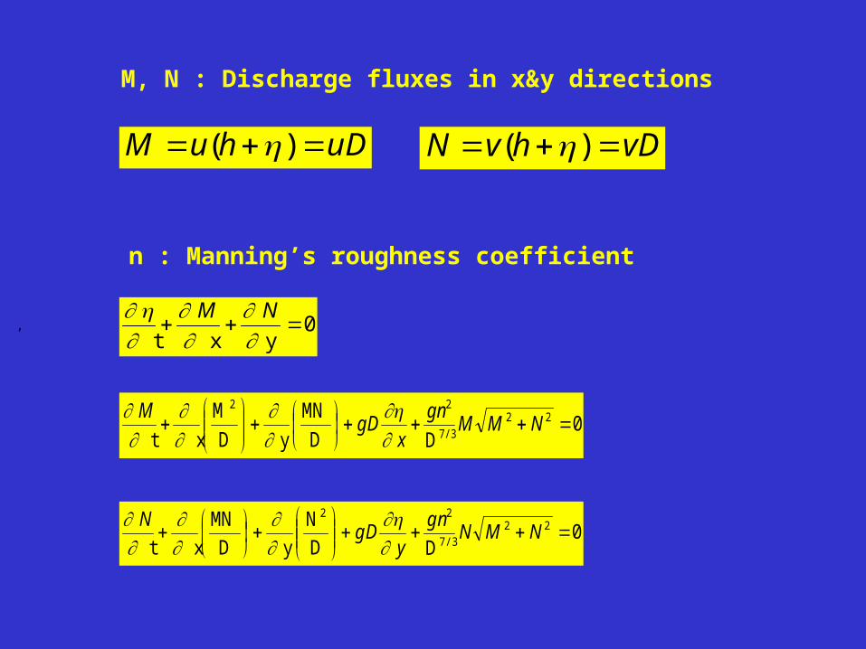
uDhuM )(
,
vDhvN )(
0y
x
t
NM
0D D
MN
y
D
M
x
t
227/3
22
NMM
gn
xgD
M
0D D
N
y
D
MN
x
t
227/3
22
NMN
gn
ygD
N
M, N : Discharge fluxes in x&y directions
n : Manning’s roughness coefficient
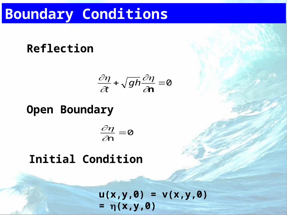
Boundary Conditions
Reflection
0n
ght
0n
Open Boundary
Initial Condition
u(x,y,0) = v(x,y,0) = (x,y,0)
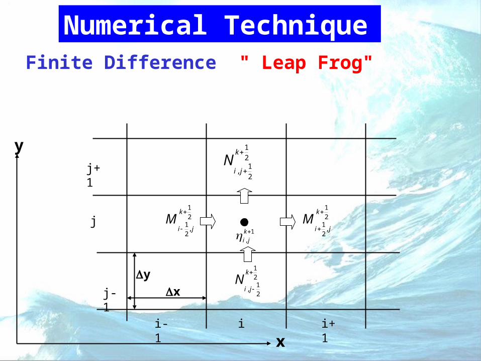
Numerical TechniqueFinite Difference " Leap Frog"
j+1
j
i
2
1
2
1,
k
jiN
21
21
,
k
jiN
2
1
,2
1
k
jiM 2
1
,2
1
k
jiM
1
,
k
ji
y
xi-1 i+1
j-1
y
x
Convective Terms
2
1
,2
1
2
2
1
,2
1
31
2
1
,2
1
2
2
1
,2
1
21
2
1
,2
3
2
2
1
,2
3
11
21
k
ji
k
ji
k
ji
k
ji
k
ji
k
ji
D
M
D
M
D
M
xD
M
x
2
1
11,2
1
2
1
1,2
12
1
1,2
1
31
2
1
,2
1
2
1
,2
12
1
,2
1
21
2
1
1,2
1
2
1
1,2
12
1
1,2
1
11
1k
ji
k
ji
k
ji
k
ji
k
ji
k
ji
k
ji
k
ji
k
ji
D
NM
D
NM
D
NM
yDMN
y
Truncation in the order of x
2
1
2
1,1
2
1
2
1,1
2
1
2
1,1
32
2
1
2
1,
2
1
2
1,
2
1
2
1,
22
2
1
2
1,1
2
1
2
1,1
2
1
2
1,1
12
1k
ji
k
ji
k
ji
k
ji
k
ji
k
ji
k
ji
k
ji
k
ji
D
NM
D
NM
D
NM
xDMN
x
21
21
,
2
21
21
,
3221
21
,
2
21
21
,
2221
23
,
2
21
23
,
12
21
k
ji
k
ji
k
ji
k
ji
k
ji
k
ji
D
N
D
N
D
N
yD
N
y
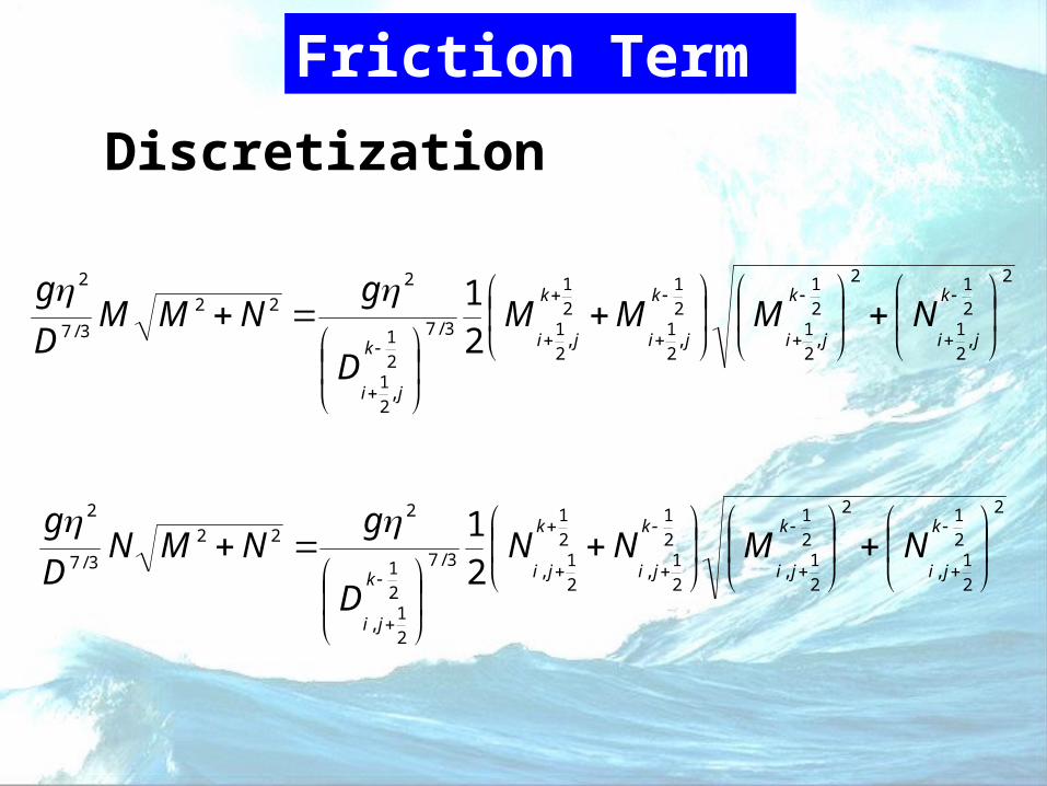
Friction Term
2
2
1
,2
1
2
2
1
,2
12
1
,2
12
1
,2
13/7
2
1
,2
1
2
22
3/7
2
21
k
ji
k
ji
k
ji
k
jik
ji
NMMM
D
gNMM
D
g
2
2
1
2
1,
2
2
1
2
1,
2
1
2
1,
2
1
2
1,
3/7
2
1
2
1,
2
22
3/7
2
21
k
ji
k
ji
k
ji
k
jik
ji
NMNN
D
gNMN
D
g
Discretization
Tunami-N2
Programme TIME : Tsunami Inundation Model Exchange
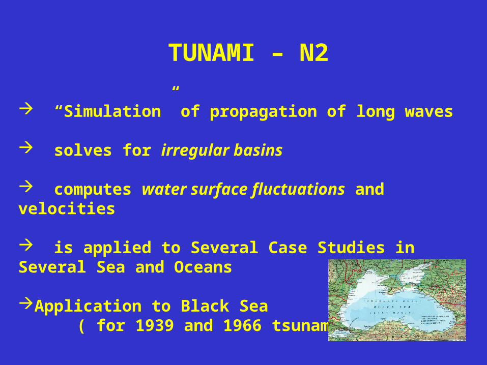
TUNAMI – N2
“Simulation” of propagation of long waves
solves for irregular basins
computes water surface fluctuations and velocities
is applied to Several Case Studies in Several Sea and Oceans
Application to Black Sea ( for 1939 and 1966 tsunamis )
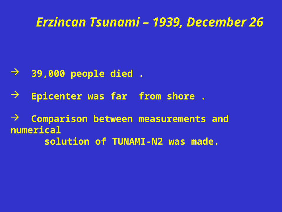
Erzincan Tsunami – 1939, December 26
39,000 people died .
Epicenter was far from shore .
Comparison between measurements and numerical solution of TUNAMI-N2 was made.
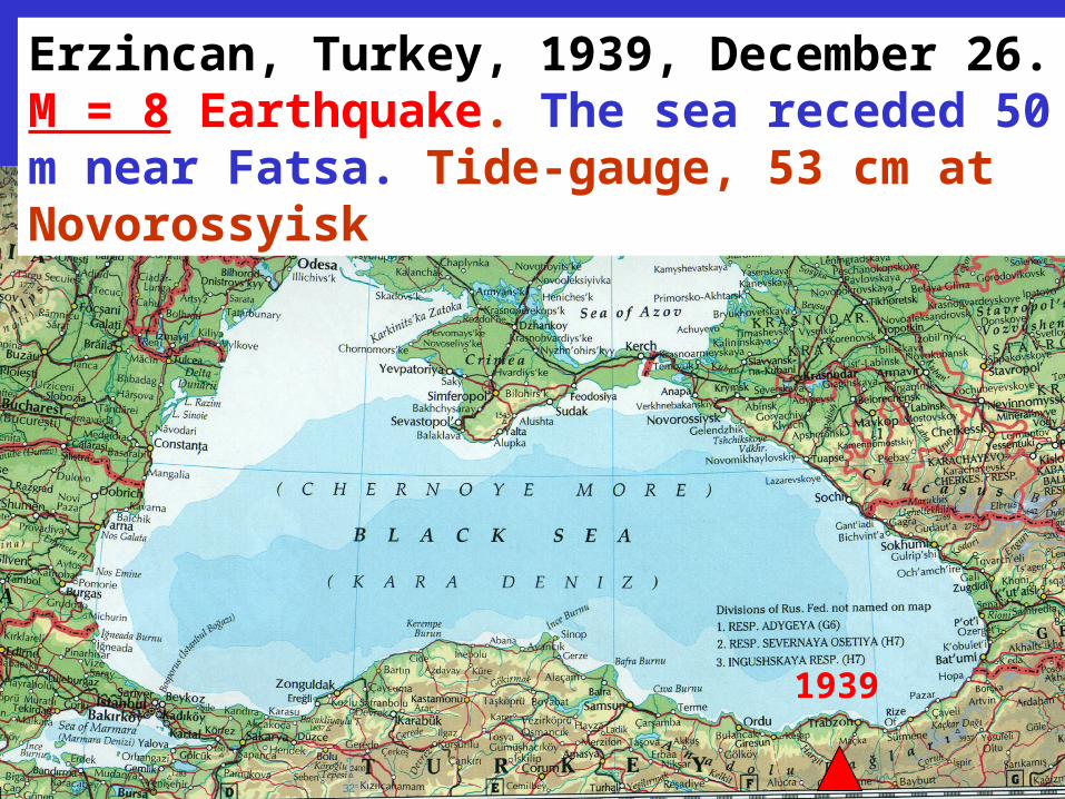
Erzincan, Turkey, 1939, December 26. M = 8 Earthquake. The sea receded 50 m near Fatsa. Tide-gauge, 53 cm at Novorossyisk
1939
1939
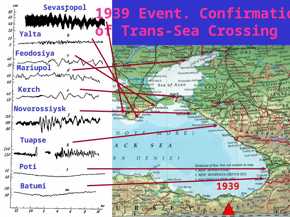
1939 Event. Confirmationof Trans-Sea Crossing
Sevastopol
Yalta
Feodosiya
Mariupol
Kerch
Novorossiysk
Tuapse
Poti
Batumi
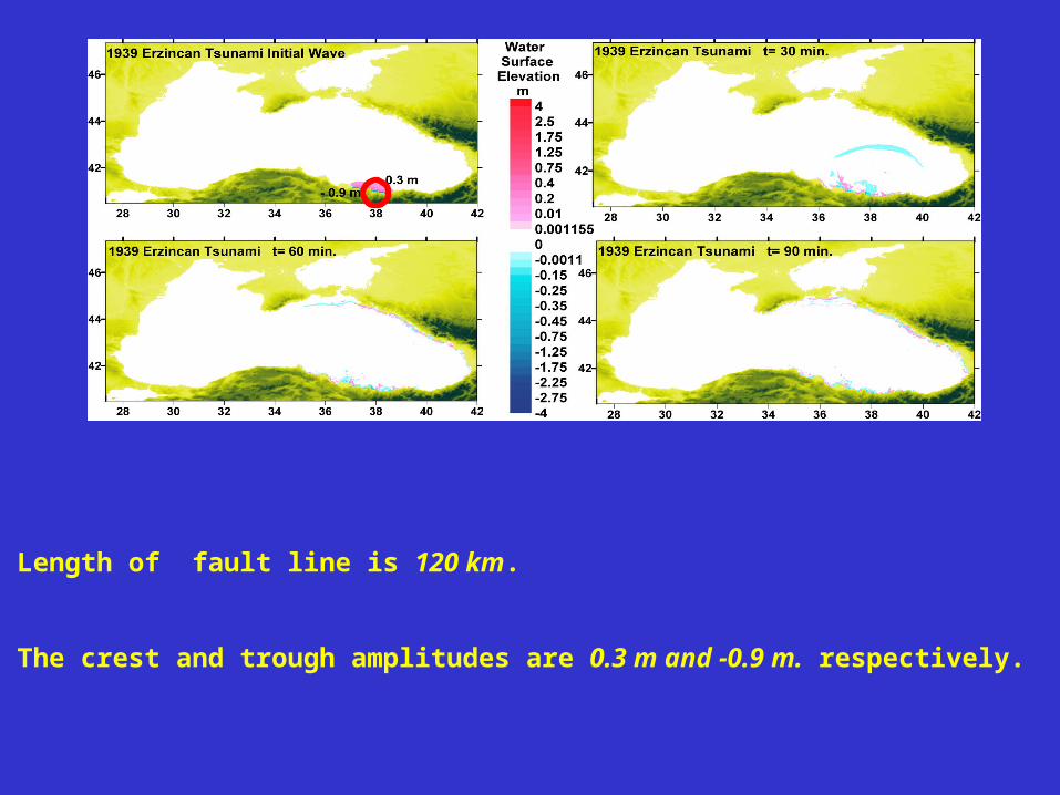
Length of fault line is 120 km.
The crest and trough amplitudes are 0.3 m and -0.9 m. respectively.
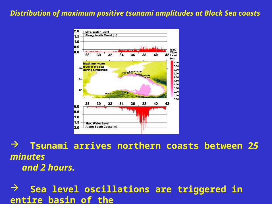
Distribution of maximum positive tsunami amplitudes at Black Sea coasts
Tsunami arrives northern coasts between 25 minutes and 2 hours.
Sea level oscillations are triggered in entire basin of the Black Sea.
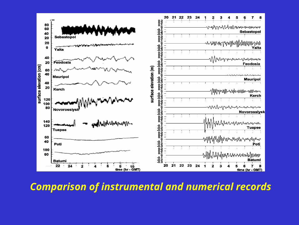
Comparison of instrumental and numerical records
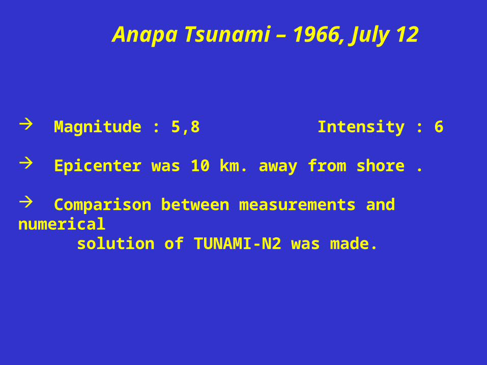
Anapa Tsunami – 1966, July 12
Magnitude : 5,8 Intensity : 6
Epicenter was 10 km. away from shore .
Comparison between measurements and numerical solution of TUNAMI-N2 was made.
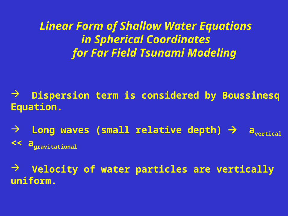
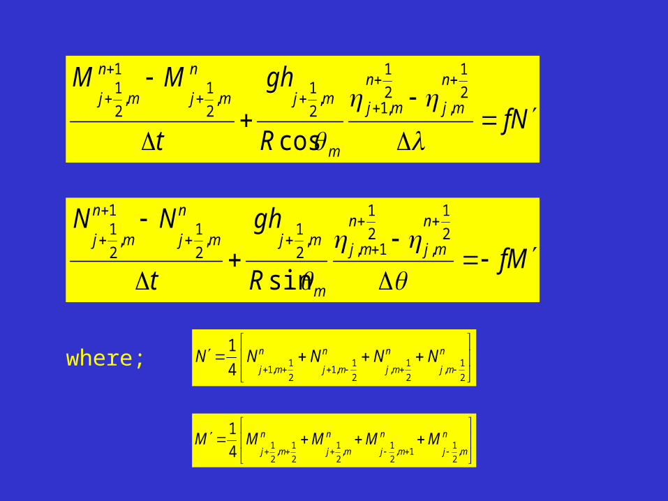
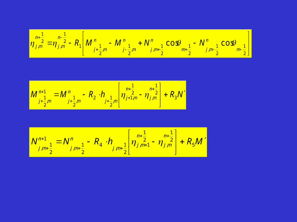
Linear Form of Shallow Water Equations in Spherical Coordinates
for Far Field Tsunami Modeling
Dispersion term is considered by Boussinesq Equation.
Long waves (small relative depth) avertical << agravitational
Velocity of water particles are vertically uniform.
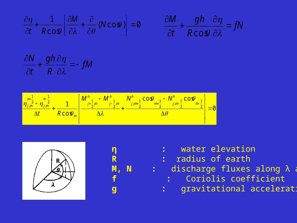
0)cos(cos
1
NM
RtfN
R
gh
t
M
cos
fMR
gh
t
N
0
coscos
cos
1 2
1
2
1,
2
1
2
1,,
2
1,
2
12
1
,2
1
,
m
n
mjm
n
mj
n
mj
n
mj
m
n
mj
n
mj
NNMM
Rt
η : water elevationR : radius of earthM, N : discharge fluxes along λ and Өf : Coriolis coefficientg : gravitational acceleration
NfR
gh
t
MM n
mj
n
mj
m
mj
n
mj
n
mj
2
1
,2
1
,1,
2
1,
2
11
,2
1
cos
MfR
gh
t
NN n
mj
n
mj
m
mj
n
mj
n
mj
2
1
,2
1
1,,
2
1,
2
11
,2
1
sin
n
mj
n
mj
n
mj
n
mjNNNNN
2
1,
2
1,
2
1,1
2
1,14
1
n
mj
n
mj
n
mj
n
mjMMMMM
,2
11,
2
1,
2
1
2
1,
2
14
1
where;
2
1
2
1,
2
1
2
1,,
2
1,
2
112
1
,2
1
, coscosm
n
mjm
n
mj
n
mj
n
mj
n
mj
n
mj NNMMR
NRhRMMn
mj
n
mjmj
n
mj
n
mj
3
2
1
,2
1
,1,
2
12,
2
11
,2
1
MRhRNNn
mj
n
mjmj
n
mj
n
mj
5
2
1
,2
1
1,
2
1,
4
2
1,
1
2
1,
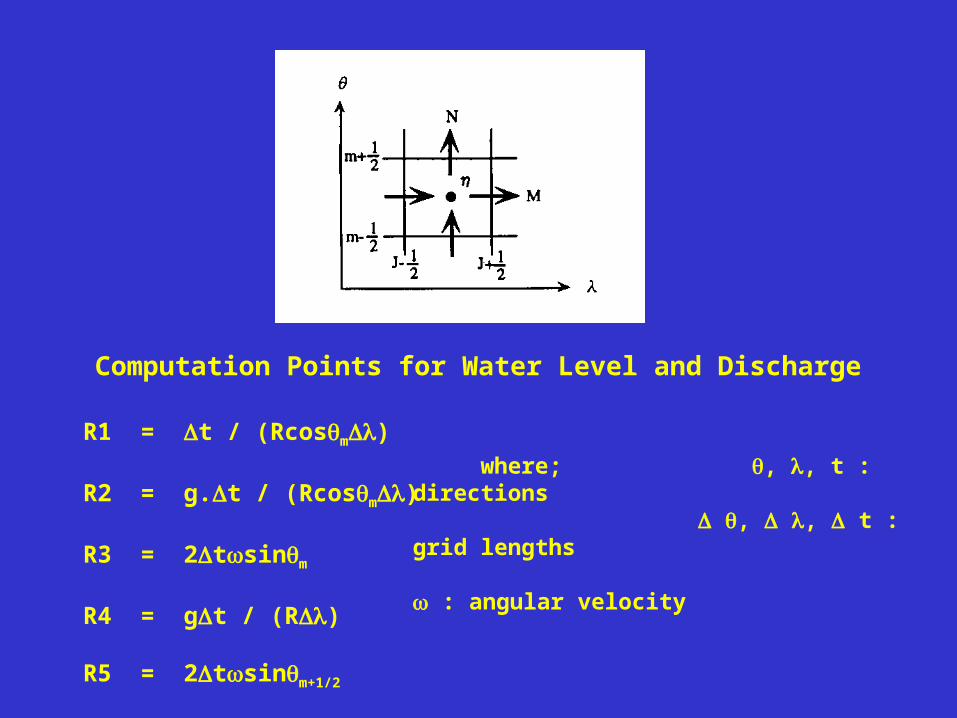
Computation Points for Water Level and Discharge
R1 = t / (Rcosm)
R2 = g.t / (Rcosm)
R3 = 2tsinm
R4 = gt / (R) R5 = 2tsinm+1/2
where; , , t : directions , , t : grid lengths : angular velocity
TWO-LAYER NUMERICAL MODEL FOR TSUNAMI GENERATION AND PROPAGATION
• The mathematical model TWOLAYER is used as a near-field tsunami modeling version with two-layer nature and combined source mechanism of landslide and fault motion
• In two-layer flow both layers interact and play a significant role in the establishment of control of the flow. The effect of the mixing or entrainment process at a front or an interface becomes important (Imamura and Imteaz, (1995)).
• Two-layer flows that occur due to an underwater landslide can be modeled using a non-horizontal bottom with a hydrostatic pressure distribution, uniform density distribution, uniform velocity distribution and negligible interfacial mixing in each layer (Watts, P., Imamura, F., Stephan. G., (2000)).
TWOLAYER
Theoretical Approach
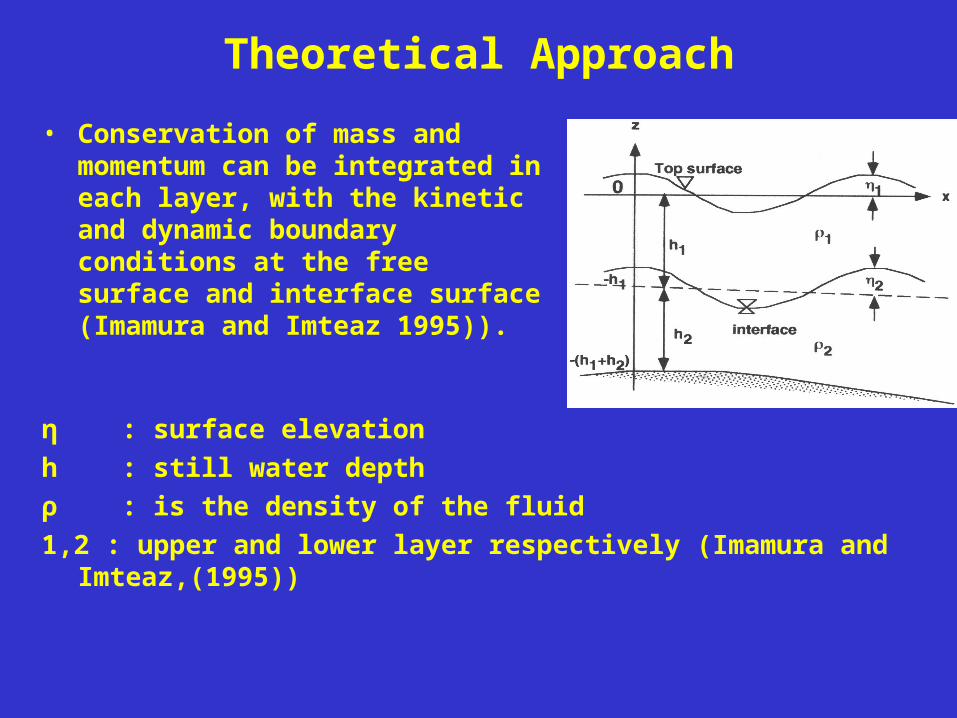
• Conservation of mass and momentum can be integrated in each layer, with the kinetic and dynamic boundary conditions at the free surface and interface surface (Imamura and Imteaz 1995)).
η : surface elevation
h : still water depth
ρ : is the density of the fluid
1,2 : upper and lower layer respectively (Imamura and Imteaz,(1995))

• The numerical model TWO-LAYER is developed in Tohoku University, Disaster Control Research Center by Prof. Imamura.
• The model computes the generation and propagation of tsunami waves generated as the result of a combined mechanism of an earthquake and an accompanying underwater landslide.
• It computes the propagation of the wave by calculating the water surface elevations and water particle velocities throughout the domain, at every time step during the simulation.
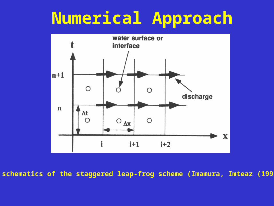
• The staggered leap-frog scheme (Shuto, Goto, Imamura, (1990)) is used to solve the governing equations.
Numerical Approach
Numerical Approach
Points schematics of the staggered leap-frog scheme (Imamura, Imteaz (1995))
Test of the Model
• The model TWO-LAYER is tested by using a regular shaped basin for modeling of generation and propagation of water waves due to underwater mass failure mechanisms.
• In order to obtain accurate results the duration and domain of simulation as well as the characteristics of the mass failure mechanism must be chosen accurately and described very precisely. For stability the time step and grid size should also be selected properly.
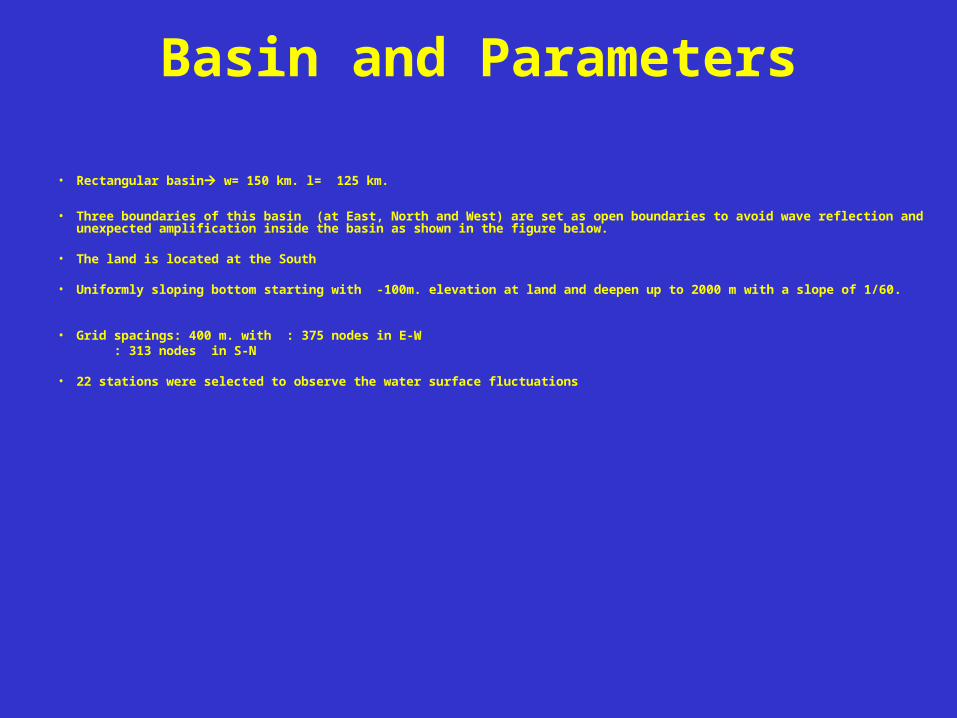
• Rectangular basin w= 150 km. l= 125 km.
• Three boundaries of this basin (at East, North and West) are set as open boundaries to avoid wave reflection and unexpected amplification inside the basin as shown in the figure below.
• The land is located at the South
• Uniformly sloping bottom starting with -100m. elevation at land and deepen up to 2000 m with a slope of 1/60.
• Grid spacings: 400 m. with : 375 nodes in E-W : 313 nodes in S-N
• 22 stations were selected to observe the water surface fluctuations
Basin and Parameters
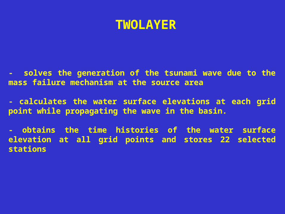
- solves the generation of the tsunami wave due to the mass failure mechanism at the source area
- calculates the water surface elevations at each grid point while propagating the wave in the basin.
- obtains the time histories of the water surface elevation at all grid points and stores 22 selected stations
TWOLAYER
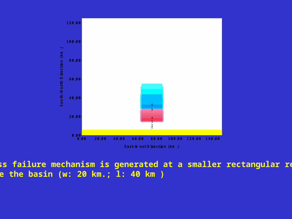
Mass failure mechanism is generated at a smaller rectangular region inside the basin (w: 20 km.; l: 40 km )
0.00 20.00 40.00 60.00 80.00 100.00 120.00 140.00
East-W est D irection (km .)
0.00
20.00
40.00
60.00
80.00
100.00
120.00
So
uth
-No
rth
Dir
ecti
on
(km
.)
1 2 3 4
5 6
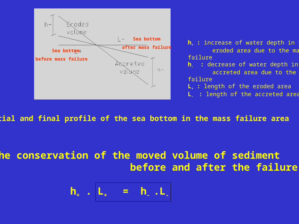
h+ : increase of water depth in the eroded area due to the mass failureh- : decrease of water depth in the accreted area due to the mass failureL+ : length of the eroded areaL- : length of the accreted area
Initial and final profile of the sea bottom in the mass failure area
The conservation of the moved volume of sediment before and after the failure
h+ . L+ = h- .L-
Sea bottom
before mass failure
Sea bottom
after mass failure

COMPARISON OF ANALYTICAL AND NUMERICAL APPROACHES FOR
LONG WAVE RUNUP
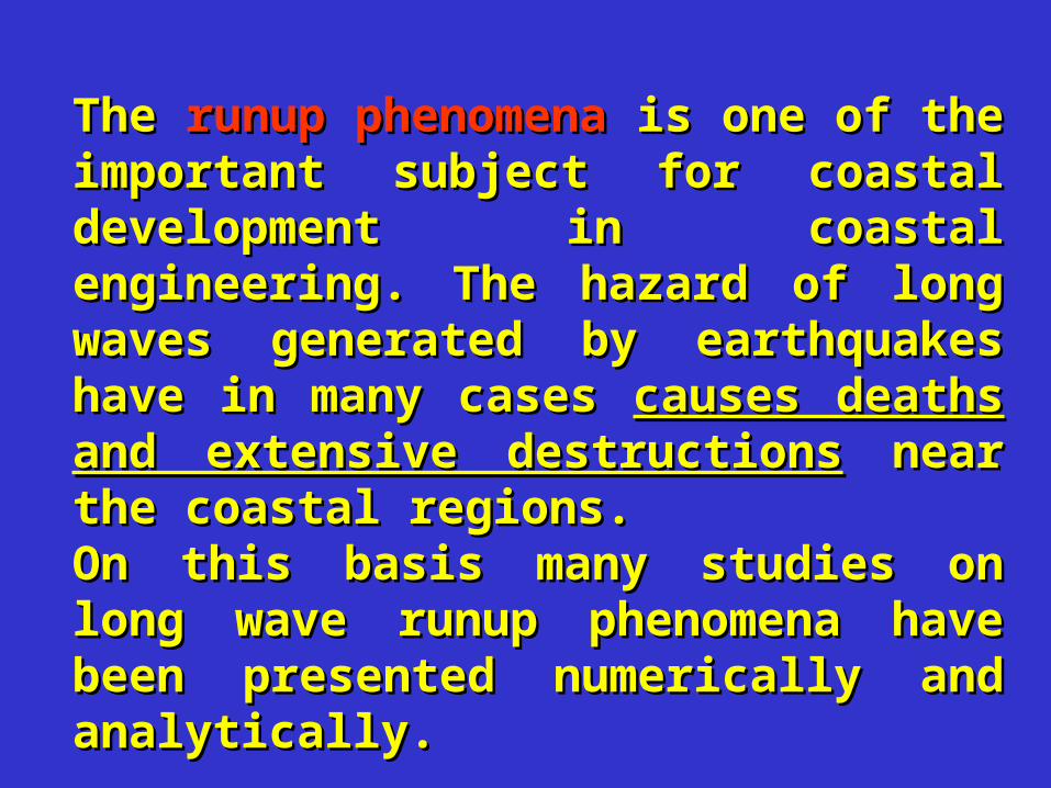
The The runup phenomenarunup phenomena is one of the is one of the important subject for coastal important subject for coastal development in coastal engineering. The development in coastal engineering. The hazard of long waves generated by hazard of long waves generated by earthquakes have in many cases earthquakes have in many cases causes causes deaths and extensive destructionsdeaths and extensive destructions near near the coastal regions. the coastal regions. On this basis many studies on long wave On this basis many studies on long wave runup phenomena have been presented runup phenomena have been presented numerically and analytically. numerically and analytically.
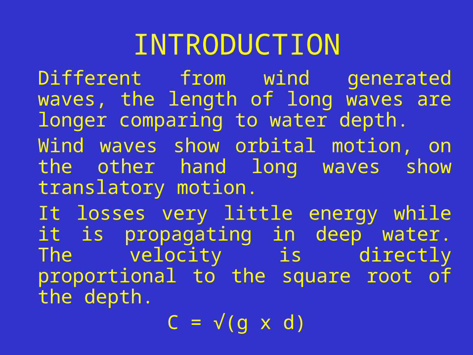
Different from wind generated waves, the length of long waves are longer comparing to water depth. Wind waves show orbital motion, on the other hand long waves show translatory motion.It losses very little energy while it is propagating in deep water. The velocity is directly proportional to the square root of the depth.
C = √(g x d)
INTRODUCTION
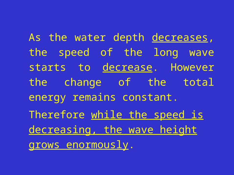
As the water depth decreases, the
speed of the long wave starts to
decrease. However the change of the
total energy remains constant.
Therefore while the speed is
decreasing, the wave height grows
enormously.
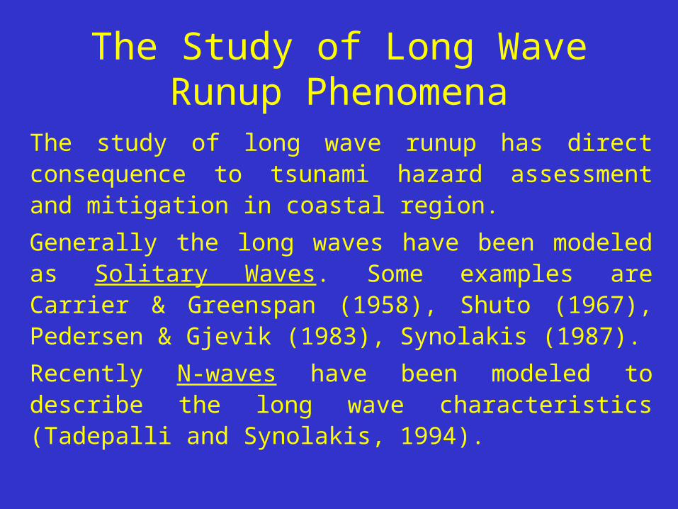
The Study of Long Wave Runup Phenomena
The study of long wave runup has direct consequence to tsunami hazard assessment and mitigation in coastal region.
Generally the long waves have been modeled as Solitary Waves. Some examples are Carrier & Greenspan (1958), Shuto (1967), Pedersen & Gjevik (1983), Synolakis (1987).
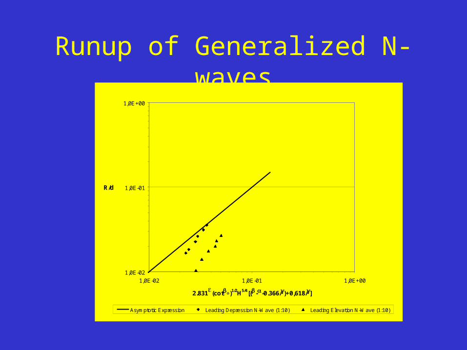
Recently N-waves have been modeled to describe the long wave characteristics (Tadepalli and Synolakis, 1994).
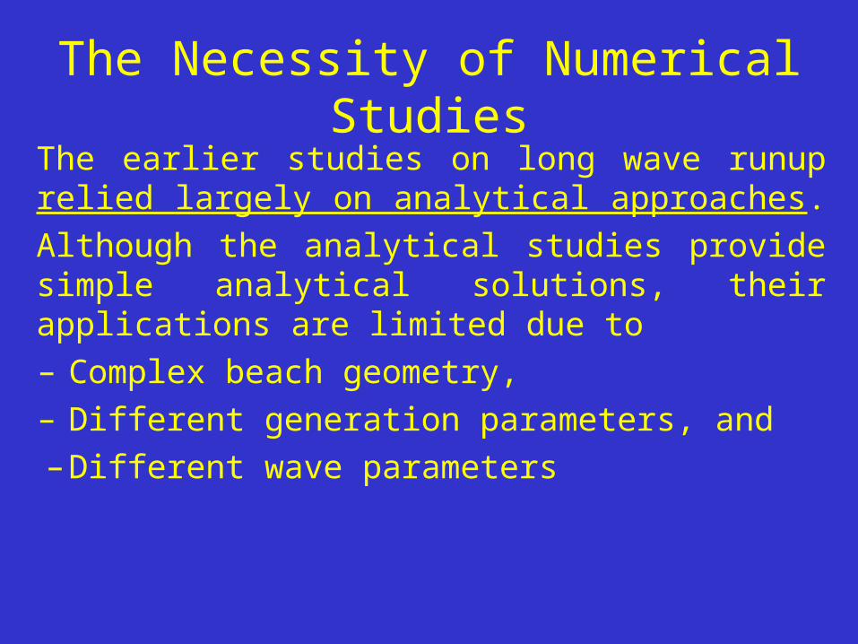
The Necessity of Numerical Studies
The earlier studies on long wave runup relied largely on analytical approaches.
Although the analytical studies provide simple analytical solutions, their applications are limited due to – Complex beach geometry,– Different generation parameters, and – Different wave parameters
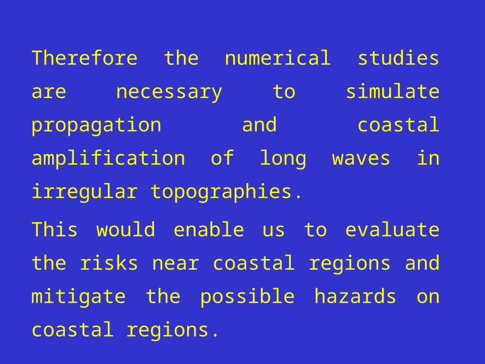
Therefore the numerical studies are
necessary to simulate propagation and
coastal amplification of long waves in
irregular topographies.
This would enable us to evaluate the risks
near coastal regions and mitigate the
possible hazards on coastal regions.
HOWEVER
The problem is to develop an adequate numerical model to describe the physical phenomena accurately.
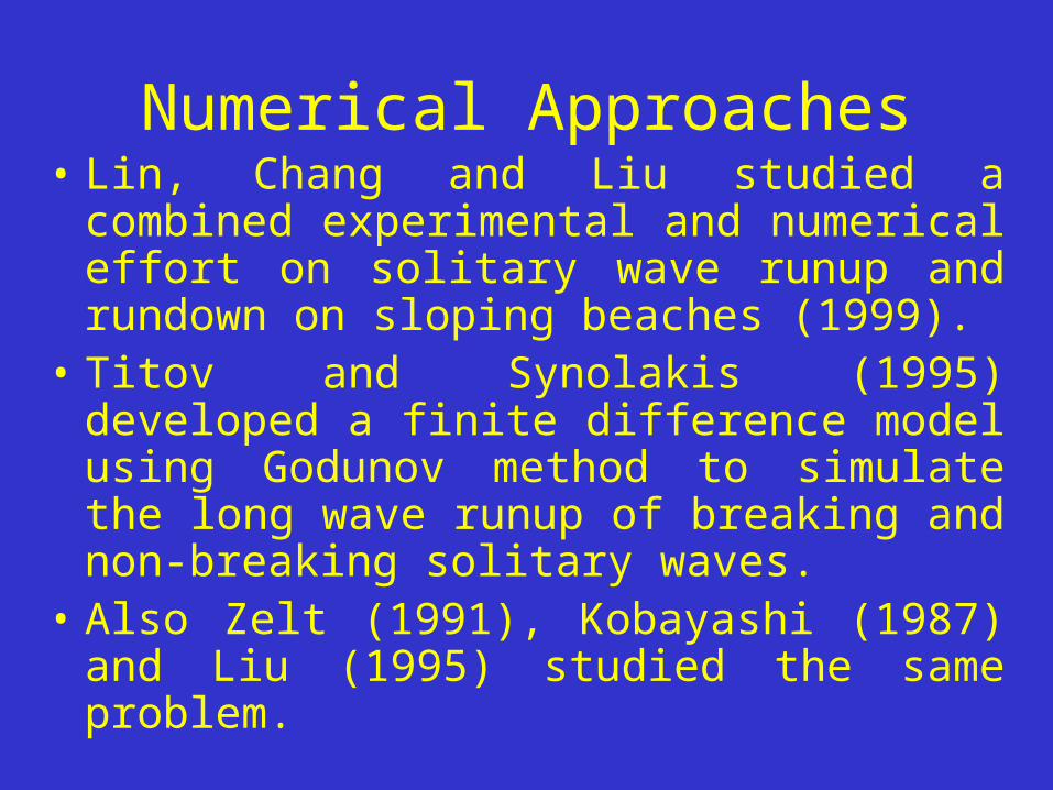
Numerical Approaches• Lin, Chang and Liu studied a combined
experimental and numerical effort on solitary wave runup and rundown on sloping beaches (1999).
• Titov and Synolakis (1995) developed a finite difference model using Godunov method to simulate the long wave runup of breaking and non-breaking solitary waves.
• Also Zelt (1991), Kobayashi (1987) and Liu (1995) studied the same problem.
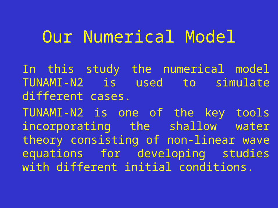
Our Numerical Model
In this study the numerical model TUNAMI-N2 is used to simulate different cases.
TUNAMI-N2 is one of the key tools incorporating the shallow water theory consisting of non-linear wave equations for developing studies with different initial conditions.
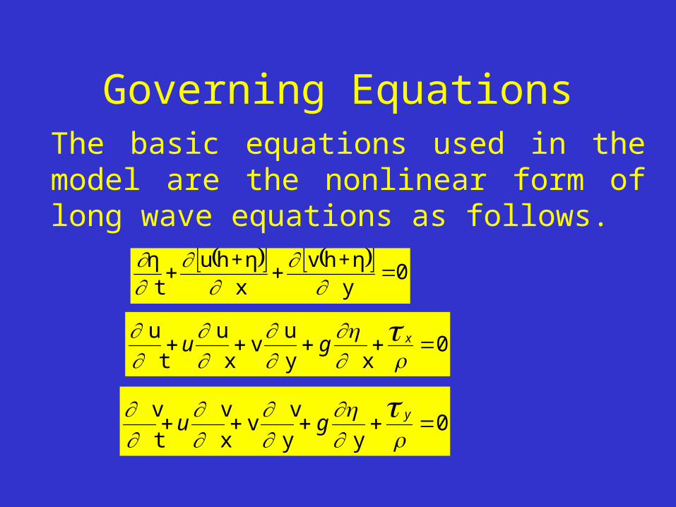
Governing EquationsThe basic equations used in the model are the nonlinear form of long wave equations as follows.
0
yη+hv
xη+hu
t η
0 x
y
u v
x
u
t
u
xgu
0y
y
vv
x
v
t
v
ygu
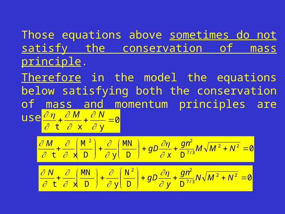
Those equations above sometimes do not satisfy the conservation of mass principle.
Therefore in the model the equations below satisfying both the conservation of mass and momentum principles are used.
0y
x
t
NM
0D D
MN
y
D
M
x
t
227/3
22
NMM
gn
xgD
M
0D D
N
y
D
MN
x
t
227/3
22
NMN
gn
ygD
N
ANALYTICAL APPROACHES FOR SOLITARY WAVE RUNUP
The key goal in analytical approaches is to
introduce a relation between Runup (R) and
Wave Height (H).
Analytical studies provide simple solutions
however their applications are generally
limited to idealized cases.
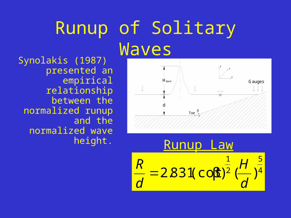
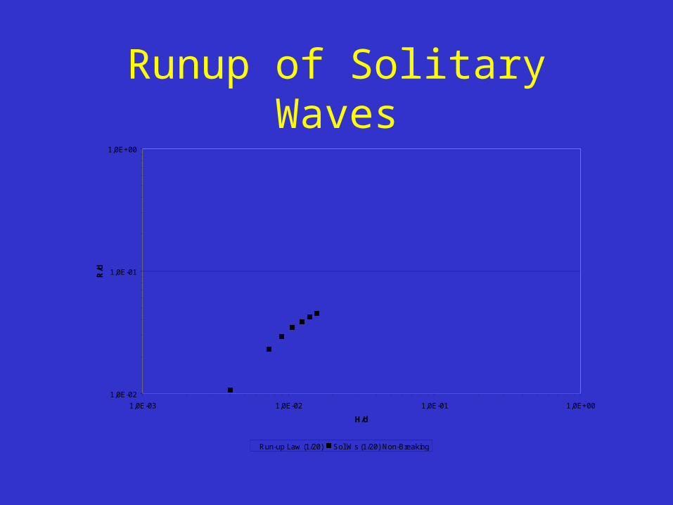
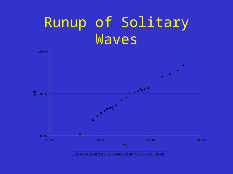
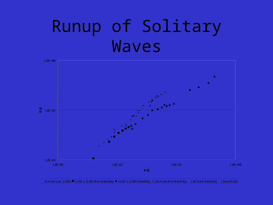
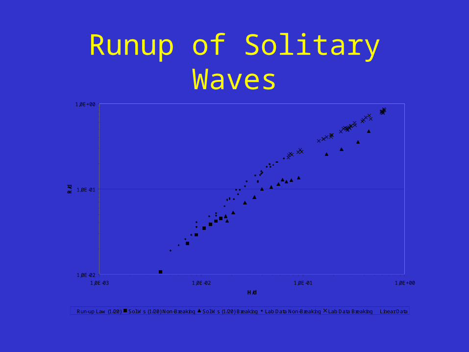
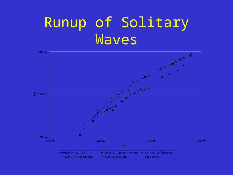
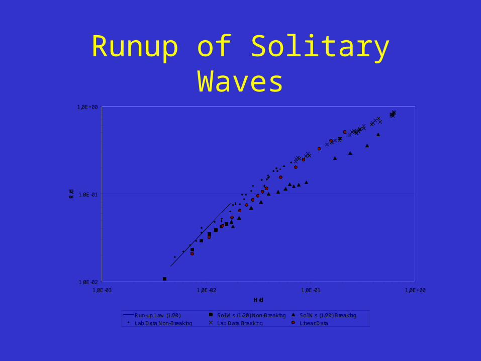
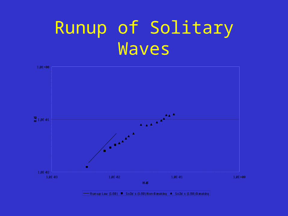
Runup of Solitary WavesSynolakis (1987)
presented an empirical
relationship between the
normalized runup and the normalized
wave height.
H
Toe
Gauges
yz
x
input
d
4
5
2
1
)()β(cot831.2d
H
d
R
Runup Law
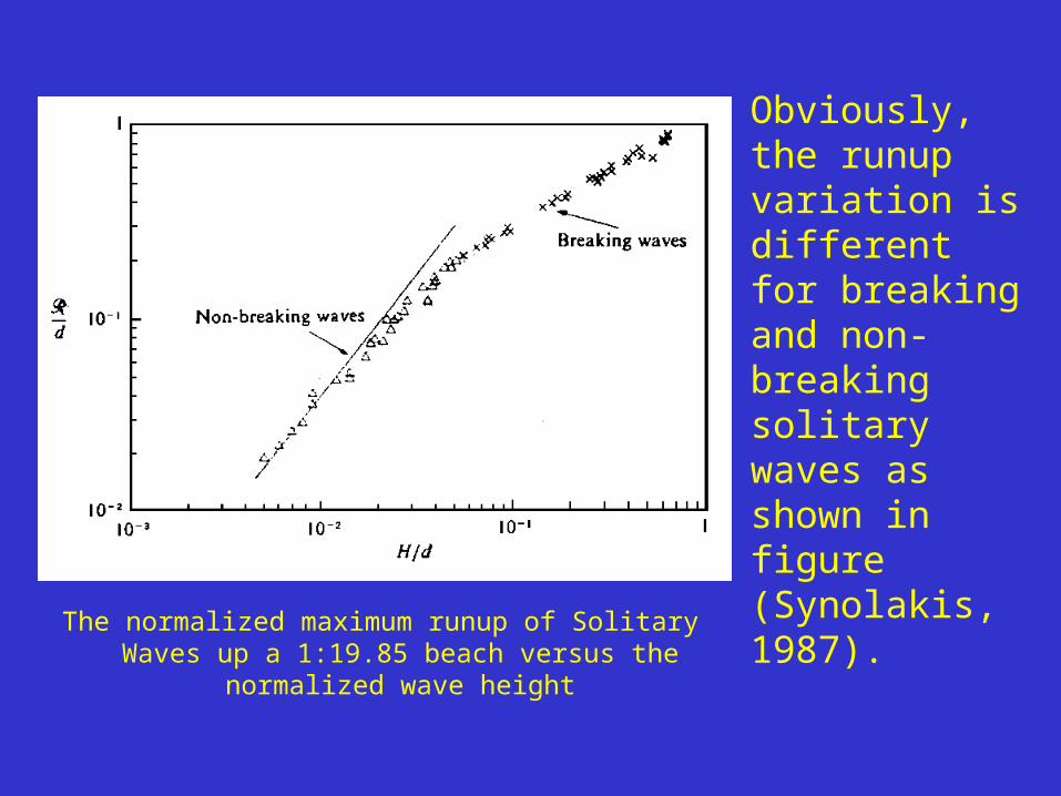
Obviously, the runup variation is different for breaking and non-breaking solitary waves as shown in figure (Synolakis, 1987).The normalized maximum runup of Solitary Waves up a
1:19.85 beach versus the normalized wave height
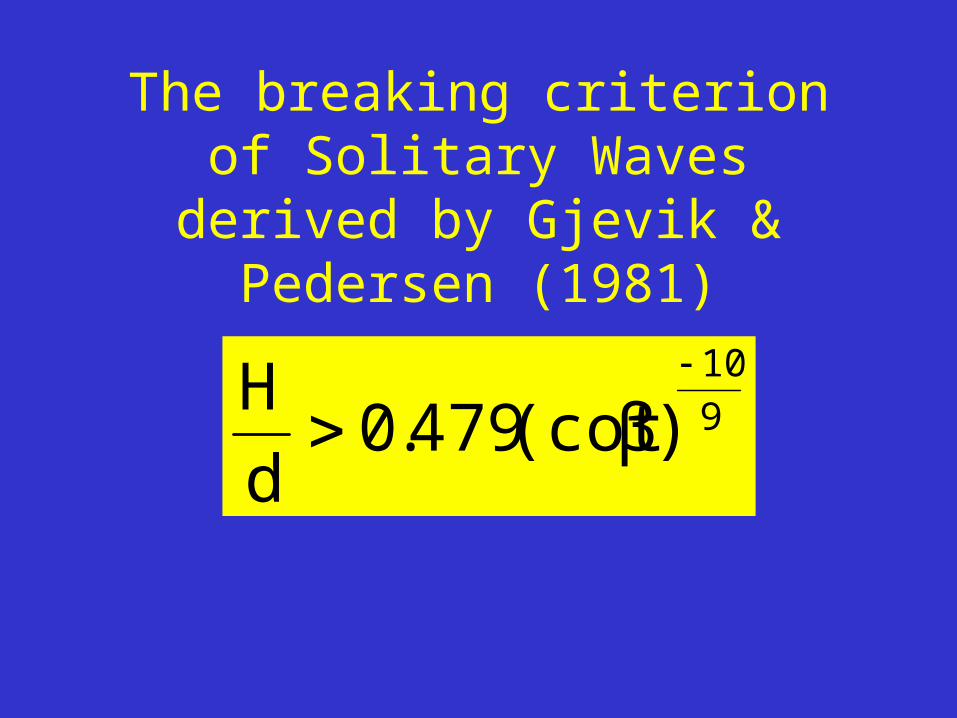
The breaking criterion of Solitary Waves derived by Gjevik &
Pedersen (1981)
9
10
)β(cot479.0d
H
Numerical Applications
For linear basins, more than 300 different
simulations were carried out.
The aim is to discuss the non-linear
numerical results with the linear and also a
few non-linear analytical approaches and
experimental studies.
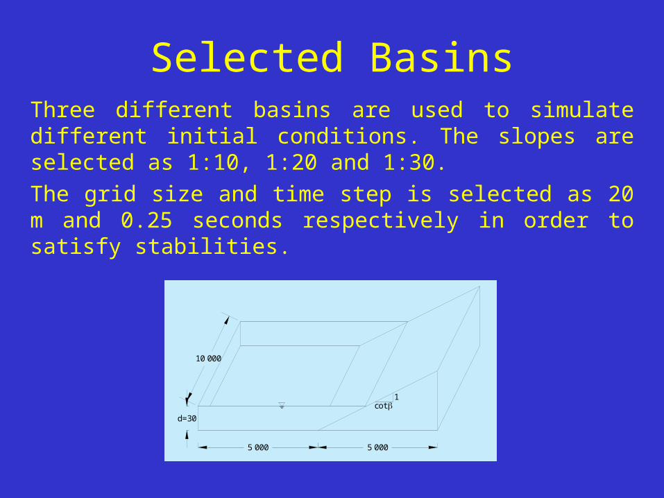
Selected BasinsThree different basins are used to simulate different initial conditions. The slopes are selected as 1:10, 1:20 and 1:30.
The grid size and time step is selected as 20 m and 0.25 seconds respectively in order to satisfy stabilities.
10 000
5 000
d=30
5 000
1cot
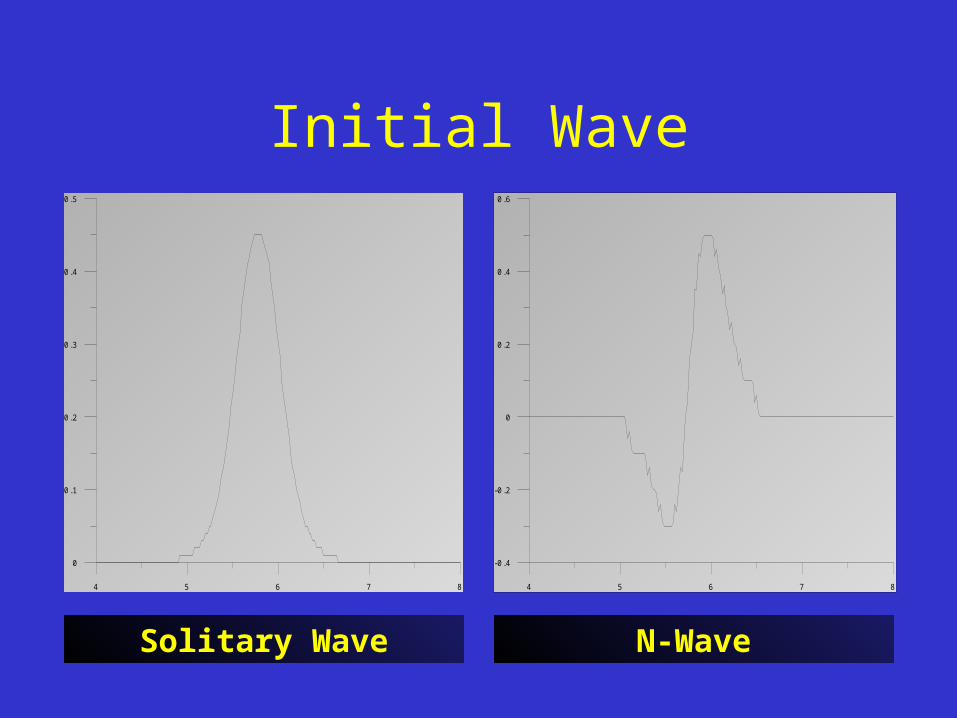
Initial Wave
4 5 6 7 8
0
0.1
0.2
0.3
0.4
0.5
4 5 6 7 8
-0.4
-0.2
0
0.2
0.4
0.6
Solitary Wave N-Wave
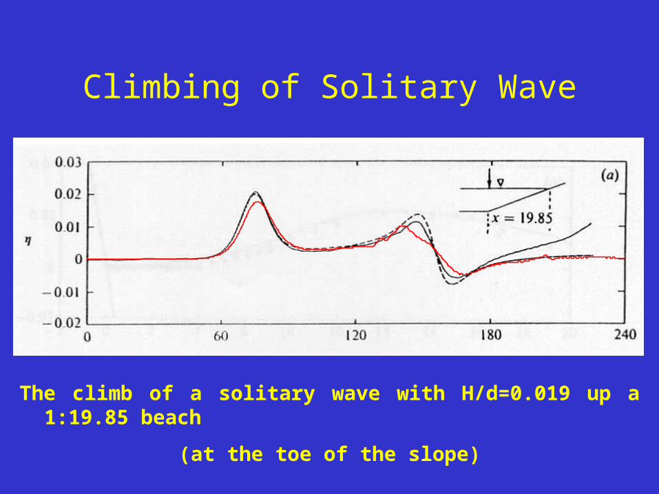
Climbing of Solitary Wave
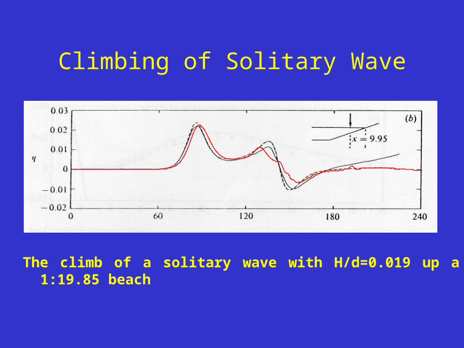
The climb of a solitary wave with H/d=0.019 up a 1:19.85 beach
(at the toe of the slope)
Climbing of Solitary Wave
The climb of a solitary wave with H/d=0.019 up a 1:19.85 beach
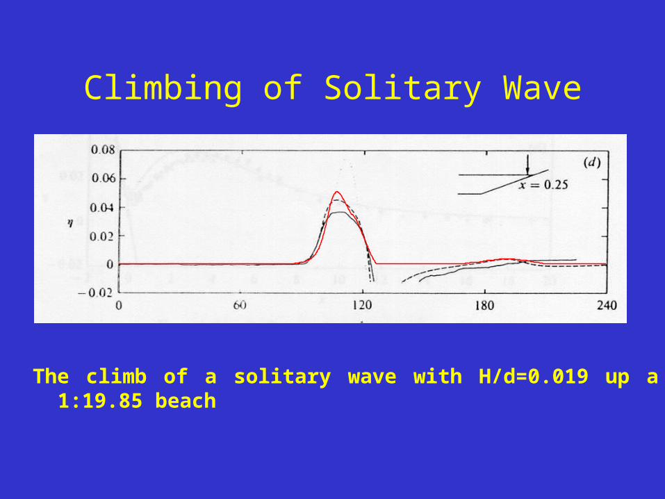
Climbing of Solitary Wave
The climb of a solitary wave with H/d=0.019 up a 1:19.85 beach
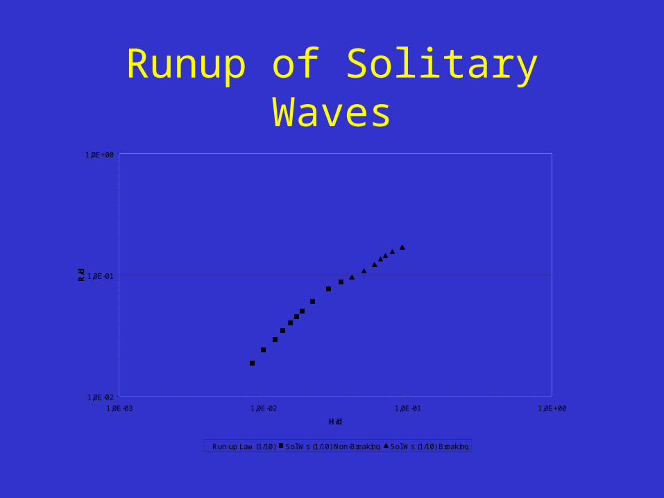
Runup of Solitary Waves
1,0E-02
1,0E-01
1,0E+00
1,0E-03 1,0E-02 1,0E-01 1,0E+00
H/d
R/d
Run-up Law (1/10) Sol Ws (1/10) Non-Breaking Sol Ws (1/10) Breaking
Runup of Solitary Waves
1,0E-02
1,0E-01
1,0E+00
1,0E-03 1,0E-02 1,0E-01 1,0E+00
H/d
R/d
Run-up Law (1/10) Sol Ws (1/10) Non-Breaking Sol Ws (1/10) Breaking
Runup of Solitary Waves
1,0E-02
1,0E-01
1,0E+00
1,0E-03 1,0E-02 1,0E-01 1,0E+00
H/d
R/d
Run-up Law (1/20) Sol Ws (1/20) Non-Breaking
Runup of Solitary Waves
1,0E-02
1,0E-01
1,0E+00
1,0E-03 1,0E-02 1,0E-01 1,0E+00
H/d
R/d
Run-up Law (1/20) Sol Ws (1/20) Non-Breaking Sol Ws (1/20) Breaking
Runup of Solitary Waves
1,0E-02
1,0E-01
1,0E+00
1,0E-03 1,0E-02 1,0E-01 1,0E+00
H/d
R/d
Run-up Law (1/20) Sol Ws (1/20) Non-Breaking Sol Ws (1/20) Breaking Lab Data Non-Breaking Lab Data Breaking Linear Data
Runup of Solitary Waves
1,0E-02
1,0E-01
1,0E+00
1,0E-03 1,0E-02 1,0E-01 1,0E+00
H/d
R/d
Run-up Law (1/20) Sol Ws (1/20) Non-Breaking Sol Ws (1/20) Breaking Lab Data Non-Breaking Lab Data Breaking Linear Data
Runup of Solitary Waves
1,0E-02
1,0E-01
1,0E+00
1,0E-03 1,0E-02 1,0E-01 1,0E+00
H/d
R/d
Run-up Law (1/20) Sol Ws (1/20) Non-Breaking Sol Ws (1/20) Breaking
Lab Data Non-Breaking Lab Data Breaking Linear Data
Runup of Solitary Waves
1,0E-02
1,0E-01
1,0E+00
1,0E-03 1,0E-02 1,0E-01 1,0E+00
H/d
R/d
Run-up Law (1/20) Sol Ws (1/20) Non-Breaking Sol Ws (1/20) Breaking
Lab Data Non-Breaking Lab Data Breaking Linear Data

Runup of Solitary Waves
1,0E-02
1,0E-01
1,0E+00
1,0E-03 1,0E-02 1,0E-01 1,0E+00
H/d
R/d
Run-up Law (1/30) Sol Ws (1/30) Non-Breaking Sol Ws (1/30) Breaking
Runup of Solitary Waves
1,0E-02
1,0E-01
1,0E+00
1,0E-03 1,0E-02 1,0E-01 1,0E+00
H/d
R/d
Run-up Law (1/30) Sol Ws (1/30) Non-Breaking Sol Ws (1/30) Breaking

Runup of Generalized N-waves
1,0E-02
1,0E-01
1,0E+00
1,0E-02 1,0E-01 1,0E+00
2.831(cot)1/2H5/4[(--0.366/)+0,618/]
R/d
Leading Depression N-Wave (1:10)

Runup of Generalized N-waves
1,0E-02
1,0E-01
1,0E+00
1,0E-02 1,0E-01 1,0E+00
2.831(cot)1/2H5/4[(--0.366/)+0,618/]
R/d
Leading Depression N-Wave (1:10) Leading Elevation N-Wave (1:10)
Runup of Generalized N-waves
1,0E-02
1,0E-01
1,0E+00
1,0E-02 1,0E-01 1,0E+00
2.831(cot)1/2H5/4[(--0.366/)+0,618/]
R/d
Asymptotic Expression Leading Depression N-Wave (1:10) Leading Elevation N-Wave (1:10)
Runup of Generalized N-waves
1,0E-02
1,0E-01
1,0E+00
1,0E-02 1,0E-01 1,0E+00
2.831(cot)1/2H5/4[(--0.366/)+0,618/]
R/d
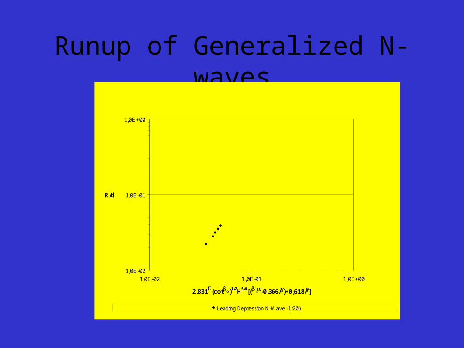
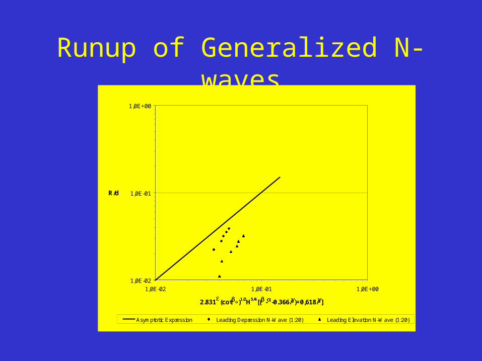
Leading Depression N-Wave (1:20)

Runup of Generalized N-waves
1,0E-02
1,0E-01
1,0E+00
1,0E-02 1,0E-01 1,0E+00
2.831(cot)1/2H5/4[(--0.366/)+0,618/]
R/d
Leading Depression N-Wave (1:20) Leading Elevation N-Wave (1:20)
Runup of Generalized N-waves
1,0E-02
1,0E-01
1,0E+00
1,0E-02 1,0E-01 1,0E+00
2.831(cot)1/2H5/4[(--0.366/)+0,618/]
R/d
Asymptotic Expression Leading Depression N-Wave (1:20) Leading Elevation N-Wave (1:20)
Runup of Generalized N-waves
1,0E-02
1,0E-01
1,0E+00
1,0E-02 1,0E-01 1,0E+00
2.831(cot)1/2H5/4[(--0.366/)+0,618/]
R/d
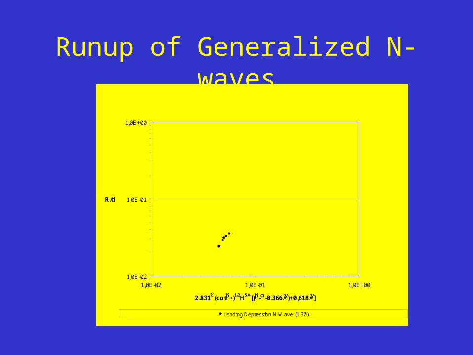
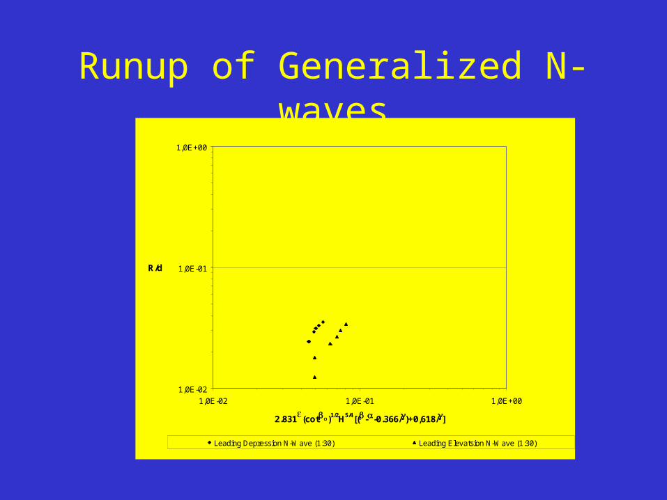
Leading Depression N-Wave (1:30)
Runup of Generalized N-waves
1,0E-02
1,0E-01
1,0E+00
1,0E-02 1,0E-01 1,0E+00
2.831(cot)1/2H5/4[(--0.366/)+0,618/]
R/d
Leading Depression N-Wave (1:30) Leading Elevatsion N-Wave (1:30)

Runup of Generalized N-waves
1,0E-02
1,0E-01
1,0E+00
1,0E-02 1,0E-01 1,0E+00
2.831(cot)1/2H5/4[(--0.366/)+0,618/]
R/d
Asymptotic Expression Leading Depression N-Wave (1:30) Leading Elevatsion N-Wave (1:30)
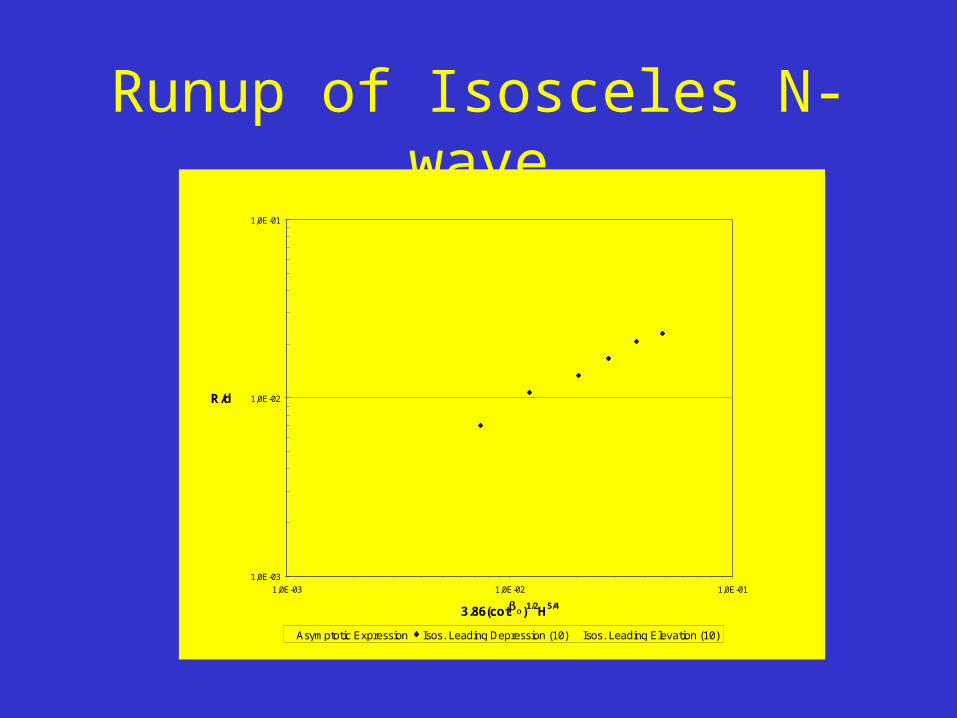
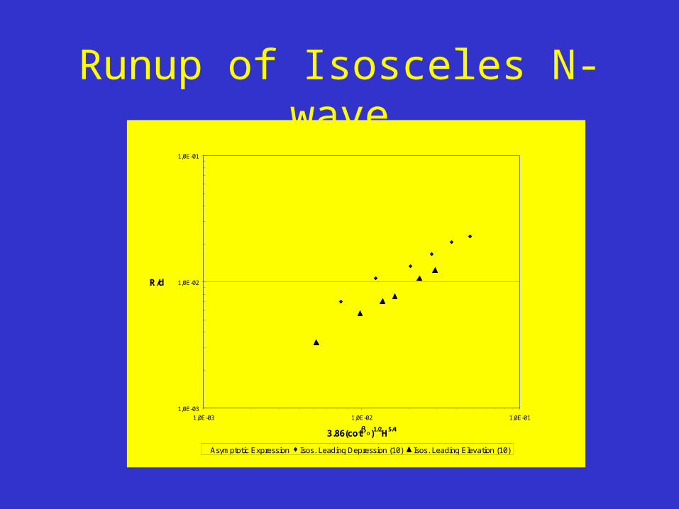
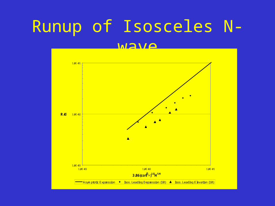
Runup of Isosceles N-wave
1,0E-03
1,0E-02
1,0E-01
1,0E-03 1,0E-02 1,0E-01
3.86(cot)1/2H5/4
R/d
Asymptotic Expression Isos. Leading Depression (10) Isos. Leading Elevation (10)
Runup of Isosceles N-wave
1,0E-03
1,0E-02
1,0E-01
1,0E-03 1,0E-02 1,0E-01
3.86(cot)1/2H5/4
R/d
Asymptotic Expression Isos. Leading Depression (10) Isos. Leading Elevation (10)
Runup of Isosceles N-wave
1,0E-03
1,0E-02
1,0E-01
1,0E-03 1,0E-02 1,0E-01
3.86(cot)1/2H5/4
R/d
Asymptotic Expression Isos. Leading Depression (10) Isos. Leading Elevation (10)
Runup of Isosceles N-wave
1,0E-03
1,0E-02
1,0E-01
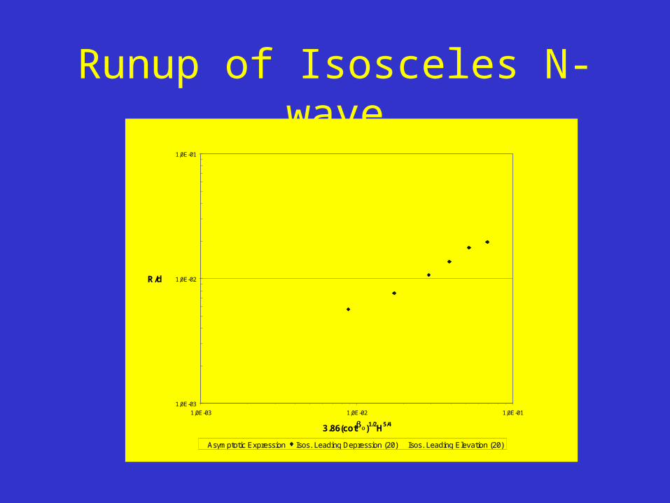
1,0E-03 1,0E-02 1,0E-01
3.86(cot)1/2H5/4
R/d
Asymptotic Expression Isos. Leading Depression (20) Isos. Leading Elevation (20)

Runup of Isosceles N-wave
1,0E-03
1,0E-02
1,0E-01
1,0E-03 1,0E-02 1,0E-01
3.86(cot)1/2H5/4
R/d
Asymptotic Expression Isos. Leading Depression (20) Isos. Leading Elevation (20)

Runup of Isosceles N-wave
1,0E-03
1,0E-02
1,0E-01
1,0E-03 1,0E-02 1,0E-01
3.86(cot)1/2H5/4
R/d
Asymptotic Expression Isos. Leading Depression (20) Isos. Leading Elevation (20)

Runup of Isosceles N-wave
1,0E-03
1,0E-02
1,0E-01
1,0E-03 1,0E-02 1,0E-01
3.86(cot)1/2H5/4
R/d
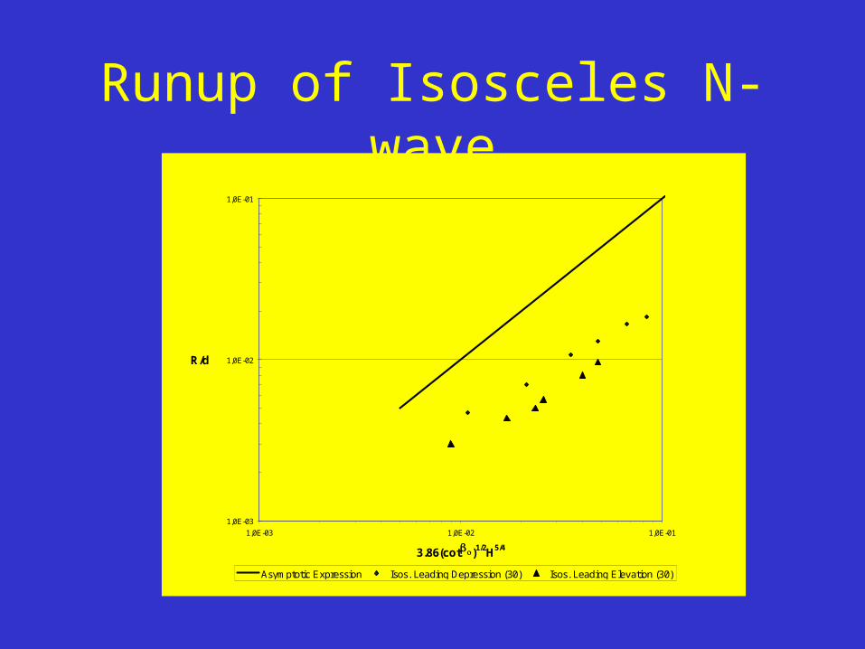
Asymptotic Expression Isos. Leading Depression (30) Isos. Leading Elevation (30)
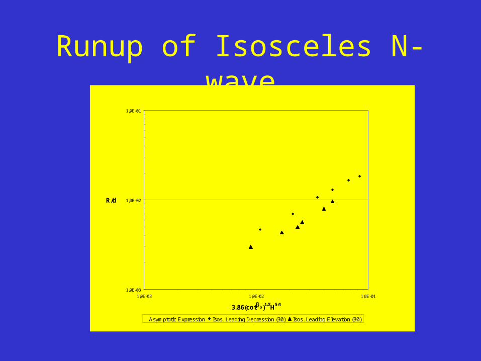
Runup of Isosceles N-wave
1,0E-03
1,0E-02
1,0E-01
1,0E-03 1,0E-02 1,0E-01
3.86(cot)1/2H5/4
R/d
Asymptotic Expression Isos. Leading Depression (30) Isos. Leading Elevation (30)
Runup of Isosceles N-wave
1,0E-03
1,0E-02
1,0E-01
1,0E-03 1,0E-02 1,0E-01
3.86(cot)1/2H5/4
R/d
Asymptotic Expression Isos. Leading Depression (30) Isos. Leading Elevation (30)
Discussion
In overall approach the numerical results show the same trend with analytical and experimental approaches.
Especially the climb of the solitary wave up a 1:19.85 slope beach shows that the numerical model results almost similar values according to the available experimental study.
For the runup calculations, the numerical model results lower runup values compared with analytical studies in both Solitary Waves and N-waves.
The trend of the relation between the normalized runup and initial wave amplitude at the toe of the slope is consistent for slopes steeper than 1:30 for non-breaking solitary wave.
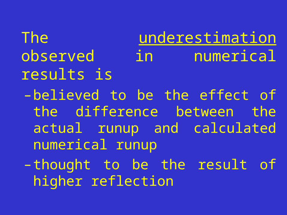
The underestimation observed in numerical results is –believed to be the effect of the
difference between the actual runup and calculated numerical runup
–thought to be the result of higher reflection