tsrt14: sensor fusion lecture 10 - linköping … sensor fusion lecture 10 ... mpf on augmented...

TSRT14: Sensor FusionLecture 10— Sensors and filter validation— Course summary— The exam

Gustaf Hendeby

[email protected]

[email protected]

TSRT14 Lecture 10 Gustaf Hendeby Spring 2018 1 / 21

Le 10: sensors and filter validation

Guest lectures:

� NIRA Dynamics— Rickard Karlsson

� Veoneer— Thomas Svantesson and Mathias Hallmen

Slides:

� Filter validation

� Course summary

� Exam


Lecture 9: summarySimultaneous Localization And Mapping (SLAM)

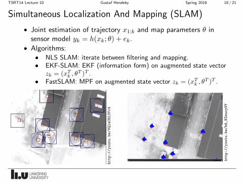
� Joint estimation of trajectory x1:k and map parameters θ insensor model yk = h(xk; θ) + ek.

� Algorithms:� NLS SLAM: iterate between filtering and mapping.� EKF-SLAM: EKF (information form) on augmented state vector

zk = (xTk , θT )T .

� FastSLAM: MPF on augmented state vector zk = (xTk , θT )T .

http://youtu.be/VQlaCHl3Yc4

http://youtu.be/hA_NZeuoy9Y



Filter Validation


Filter and Model Validation

A filter assumes correct

� motion model

� sensor model

How to validate these?

Key ideas:

� Sensitivity analysis

� Ground truth analysis


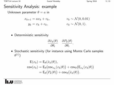
Sensitivity Analysis: exampleUnknown parameter θ = a in

xk+1 = axk + vk, vk ∼ N (0, 0.01)

yk = xk + ek, ek ∼ N (0, 1).

� Deterministic sensitivity

∂xk(θ)

∂θi

∂Pk(θ)

∂θi.

� Stochastic sensitivity (for instance using Monte Carlo samplesθ(i))

E(xk) = Eθ(xk(θ)),

cov(xk) = Eθ(covxk(xk|θ)

)+ covθ

(Exk(xk|θ)

)= Eθ

(Pk(θ)

)+ covθ

(xk(θ)

).


Ground-Truth Analysis

Ground truth never available. However, a state sequence x1:N goodenough can be obtained using:

� better models (more states, less approximations andlinearizations);

� better sensors (reference IMU);

� more sensors (GPS for non-GPS applications);

� better filters (smoothers where filters will be used, PF whereEKF will be used, . . . ).


Ground-Truth AnalysisHow to use ground-truth to validate a filter?

� The “I’m feeling lucky” test statistic

T =

N∑k=1

(xk − x0k

)TP−1k

(xk − x0k

).

� Separate sensor model validation

T =

N∑k=1

(yk − h(xok)

)TR−1

(yk − h(xok)

).

� Separate motion model validation

T =

N∑k=1

(x0k+1 − f(xok)

)TQ−1

(x0k+1 − f(x0k

).

� Validate Q and R.

Course Summary


Parameter Estimation: least squares (LS)

Linear Model

y = Hx+ e, cov(e) = R.

� WLS minimizes the loss function

V WLS(x) = (y −Hx)TR−1(y −Hx).

� WLS solution

x =(HTR−1H

)−1HTR−1y, P =

(HTR−1H

)−1.


Parameter Estimation: least squares (LS)

Nonlinear Model

y = h(x) + e, cov(e) = R.

� NWLS minimizes the loss function

V nwls(x) =(y − h(x)

)TR−1

(y − h(x)

)� Solve using optimization methods

xnwls = arg minx

V nwls(x)


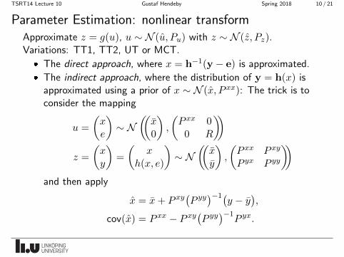
Parameter Estimation: nonlinear transformApproximate z = g(u), u ∼ N (u, Pu) with z ∼ N (z, Pz).Variations: TT1, TT2, UT or MCT.

� The direct approach, where x = h−1(y − e) is approximated.

� The indirect approach, where the distribution of y = h(x) isapproximated using a prior of x ∼ N (x, P xx): The trick is toconsider the mapping

u =

(xe

)∼ N

((x0

),

(P xx 0

0 R

))z =

(xy

)=

(x

h(x, e)

)∼ N

((xy

),

(P xx P xy

P yx P yy

))and then apply

x = x+ P xy(P yy

)−1(y − y

),

cov(x) = P xx − P xy(P yy

)−1P yx.


Fusing Estimates

� The fusion formula for two independent estimates is

E(x1) = E(x2) = x, cov(x1) = P1, cov(x2) = P2 ⇒

x = P(P−11 x1 + P−12 x2

), P =

(P−11 + P−12

)−1.

� If the estimates are not independent, P is larger than indicated.Use Safe fusion!


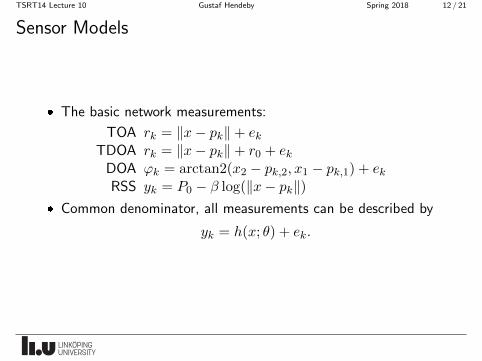
Sensor Models

� The basic network measurements:

TOA rk = ‖x− pk‖+ ekTDOA rk = ‖x− pk‖+ r0 + ek

DOA ϕk = arctan2(x2 − pk,2, x1 − pk,1) + ekRSS yk = P0 − β log(‖x− pk‖)

� Common denominator, all measurements can be described by

yk = h(x; θ) + ek.


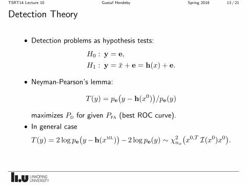
Detection Theory

� Detection problems as hypothesis tests:

H0 : y = e,

H1 : y = x+ e = h(x) + e.

� Neyman-Pearson’s lemma:

T (y) = pe(y − h(x0)

)/pe(y)

maximizes Pd for given Pfa (best ROC curve).

� In general case

T (y) = 2 log pe(y−h(xml)

)− 2 log pe(y) ∼ χ2

nx

(x0,T I(x0)x0

).


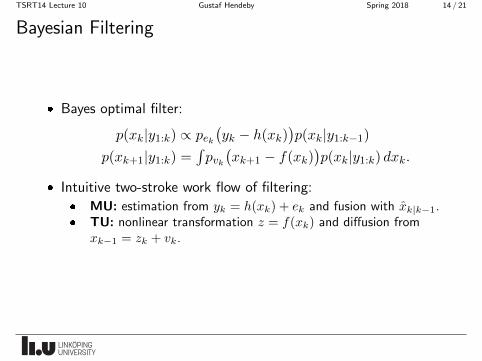
Bayesian Filtering

� Bayes optimal filter:

p(xk|y1:k) ∝ pek(yk − h(xk)

)p(xk|y1:k−1)

p(xk+1|y1:k) =∫pvk(xk+1 − f(xk)

)p(xk|y1:k) dxk.

� Intuitive two-stroke work flow of filtering:

� MU: estimation from yk = h(xk) + ek and fusion with xk|k−1.� TU: nonlinear transformation z = f(xk) and diffusion from

xk−1 = zk + vk.


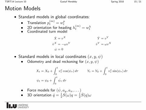
Motion Models

� Standard models in global coordinates:

� Translation p(m)t = wp

t

� 2D orientation for heading h(m)t = wh

t� Coordinated turn model

X = vX Y = vY

vX = −ωvY vY = ωvX

ω = 0

� Standard models in local coordinates (x, y, ψ)� Odometry and dead reckoning for (x, y, ψ)

Xt = X0 +

∫ t

0vxτ cos(ψτ ) dτ Yt = Y0 +

∫ t

0vxτ sin(ψτ ) dτ

ψt = ψ0 +

∫ t

0ψτ dτ

� Force models for (ψ, ay, ax, . . . )� 3D orientation q = 1

2S(ω)q = 12 S(q)ω


Filtering: Kalman filter (approximations)

Key tool for a unified derivation of KF, EKF, UKF.(XY

)∼ N

((µxµy

),

(Pxx PxyPxy Pyy

))⇒ (X|Y = y) ∼ N (µx + PxyP

−1yy (y − µy), Pxx − PxyP−1

yy Pyx).

The Kalman gain is in this notation given by Kk = PxyP−1yy .

� In KF, Pxy and Pyy follow from a linear Gaussian model.

� In EKF, Pxy and Pyy can be computed from a linearized model(requires analytic gradients).

� In EKF and UKF, Pxy and Pyy computed by NLT fortransformation of (xT , vT )T and (xT , eT )T , respectively. Nogradients required, just function evaluations.


Filtering: SIS PF AlgorithmChoose the number of particles N , a proposal density

q(x(i)k |x

(i)0:k−1, y1:k), and a threshold Nth (for instance Nth = 2

3N).

� Initialization: Generate x(i)0 ∼ px0 , i = 1, . . . , N .

Iterate for k = 1, 2, . . . :

1. Measurement update: For i = 1, 2, . . . , N :

w(i)k|k = w

(i)k|kp(yk|x

(i)k ), and normalize w

(i)k|k.

2. Estimation: MMSE xk|k ≈∑N

i=1w(i)k x

(i)k|k.

3. Resampling: Resample with replacement whenNeff = 1∑

i(w(i)k|k)

2< Nth.

4. Prediction: Generate samples x(i)k+1 ∼ q(xk|x

(i)k−1, yk),

update the weights w(i)k+1|k ∝ w

(i)k|k

p(x(i)k |x

(i)k−1)

q(x(i)k |x

(i)k−1,yk)

,

and normalize w(i)k+1|k.


Simultaneous Localization And Mapping (SLAM)

� Joint estimation of trajectory x1:k and map parameters θ insensor model yk = h(xk; θ) + ek.

� Algorithms:� NLS SLAM: iterate between filtering and mapping.� EKF-SLAM: EKF (information form) on augmented state vector

zk = (xTk , θT )T .

� FastSLAM: MPF on augmented state vector zk = (xTk , θT )T .





The Exam


The Exam: tools

Allowed Tools

� The course book: Statistical Sensor Fusion by F. Gustafsson.

Normal study notes in the books are allowed!

Made Available Digitally

� Lecture slides

� Signal and Systems toolbox manual


The Exam: advice

General Advice

� Read through all exercises and prioritize, before getting started.

� Make sure to motivate every step of your solution carefully!

� Comment nontrivial steps in any code you write; includingmodel choices and tuning

� Separate papers for all exercises, keep the papers for eachexercise together.

GOOD LUCK!

Gustaf [email protected]

www.liu.se

mailto:[email protected]

www.liu.se

tsrt14: sensor fusion lecture 10 - linköping … sensor fusion lecture 10 ... mpf on augmented...

Documents