tropospheric ozone at tropical and middle latitudes derived...

Tropospheric ozone at tropical and middle latitudes derived from

TOMS/MLS residual: Comparison with a global model

S. ChandraNASA Goddard Space Flight Center, Greenbelt, Maryland, USA

J. R. ZiemkeGoddard Earth Sciences and Technology Center, University of Maryland, Baltimore County, Baltimore, Maryland, USA

R. V. Martin1

Department of Earth and Planetary Sciences Division of Engineering and Applied Sciences, Harvard University, Cambridge,Massachusetts, USA

Received 5 September 2002; revised 11 December 2002; accepted 8 January 2003; published 13 May 2003.

[1] The tropospheric ozone residual method is used to derive zonal maps of troposphericcolumn ozone using concurrent measurements of total column ozone from Nimbus 7 andEarth Probe (EP) Total Ozone Mapping Spectrometer (TOMS) and stratospheric columnozone from the Microwave Limb Sounder (MLS) instrument on the Upper AtmosphereResearch Satellite (UARS). Our study shows that the zonal variability in TOMS totalcolumn ozone at tropical and subtropical latitudes is mostly of tropospheric origin. Theseasonal and zonal variability in tropospheric column ozone (TCO), derived from theTOMS/MLS residual, is consistent with that derived from the convective cloud differentialmethod and ozonesonde measurements in regions where these data overlap. A comparisonof TCO derived from the TOMS/MLS residual and a global three-dimensional model oftropospheric chemistry (GEOS-CHEM) for 1996–1997 shows good agreement in thetropics south of the equator. Both the model and observations show similar zonal andseasonal characteristics including an enhancement of TCO in the Indonesian regionassociated with the 1997 El Nino. Both show the decline of the wave-1 pattern from thetropics to the extratropics as lightning activity and the Walker circulation decline. Bothshow enhanced ozone in the downwelling branches of the Hadley Circulation near ±30o.Model and observational differences increase with latitude during winter andspring. INDEX TERMS: 0365 Atmospheric Composition and Structure: Troposphere—composition and

chemistry; 0368 Atmospheric Composition and Structure: Troposphere—constituent transport and chemistry;

3309 Meteorology and Atmospheric Dynamics: Climatology (1620); 3319 Meteorology and Atmospheric

Dynamics: General circulation; 3360 Meteorology and Atmospheric Dynamics: Remote sensing; KEYWORDS:

biomass burning, tropospheric ozone, stratospheric ozone, El Nino, global circulation model, tropopause

Citation: Chandra, S., J. R. Ziemke, and R. V. Martin, Tropospheric ozone at tropical and middle latitudes derived from TOMS/MLS

residual: Comparison with a global model, J. Geophys. Res., 108(D9), 4291, doi:10.1029/2002JD002912, 2003.

1. Introduction

[2] Many of the current techniques for deriving tropo-spheric ozone from satellite measurements are limited totropical latitudes [Jiang and Yung, 1996; Kim and New-church, 1996; Hudson and Thompson, 1998; Ziemke et al.,1998, 2001; Thompson and Hudson, 1999; Kim et al.,2001]. They are based on the tropospheric ozone residual(TOR) method, which derives tropospheric column ozone(TCO) by subtracting concurrent measurements of strato-

spheric column ozone (SCO) from total column ozonemeasured by the TOMS instrument [Fishman and Larsen,1987]. J. Fishman and his colleagues [Fishman and Larsen,1987; Fishman et al., 1990], who first introduced the TORconcept, used concurrent total column ozone measurementsfrom TOMS instrument and SCO from SAGE (Strato-spheric Aerosol and Gas Experiment) instrument to deriveTCO. SAGE, being an occultation measuring instrumentcould not be used for anything other than climatologicalstudies. Fishman and Balok [1999] have attempted toaccount for this shortcoming by replacing SAGE profileswith profiles derived from the solar backscatter ultraviolet(SBUV) measurements. Unlike SAGE, the SBUV profilesprovide daily global maps of SCO with the caveat thatSBUV has a limited profile information in the lowest threeUmkehr layers from the ground to 63 hPa. Assuming that

JOURNAL OF GEOPHYSICAL RESEARCH, VOL. 108, NO. D9, 4291, doi:10.1029/2002JD002912, 2003

1Now at Harvard-Smithsonian Center for Astrophysics, Cambridge,Mass, 02138, USA.

Copyright 2003 by the American Geophysical Union.0148-0227/03/2002JD002912$09.00

ACH 14 - 1

the integrated column ozone amount from ground to 63 hPaare correctly measured by SBUV, Fishman and Balok[1999] applied a normalization correction to SBUV profilemeasurements using ozonesonde climatology.[3] The CCD technique [Ziemke et al., 1998], which is

another version of TORmethodology, takes advantage of thefact that for UV measuring instruments, such as TOMS,optically thick clouds obscure ozone below. Therefore, onecan make a fairly accurate estimate of SCO using highreflecting convective cloud scenes (R > 0.9) near thetropopause in the tropical Pacific region. The CCD methodfurther assumes that the SCO is zonally invariant within15�N and 15�S. TCO is calculated using the total columnsdetermined from the low reflecting scenes (R < 0.2) and thestratospheric columns using high reflecting scenes (R > 0.9).[4] Chandra et al. [2002] and Martin et al. [2002] have

shown that most of the observed characteristics of ozonetime series, derived from the CCD technique, are wellcharacterized by the GEOS-CHEM 3-D tropospheric chem-istry and transport model. These characteristics includeseasonal variations and anomalously large increases inTCO in the Indonesian region during September–December1997, following large scale forest fires and Savanna burning[Chandra et al., 1998; Thompson et al., 2001]. El Ninoinduced changes in tropospheric ozone, derived from theCCD technique, were also analyzed by Sudo and Takahashi[2001], using a 3-D photochemical model developed at theCenter for Climate Research, University of Tokyo, Japan[Sudo et al., 2002]. They were able to simulate most of theobserved changes in tropospheric ozone related to 1997 ElNino and concluded, as did Chandra et al. [1998, 2002],that both the biomass burning and the changes in meteoro-logical conditions (e.g., low convective activity, sparseprecipitation, dry air condition, enhanced transport fromstratosphere) contributed almost equally to the observedenhancement in tropospheric ozone.[5] The comparison of the model and CCD tropospheric

ozone has not been very satisfactory north of the equator inthe African region. During the 1996–1997 period, observedTCO tends to have a broad peak in late fall (September–November) and a deep minimum in early spring (February–March) similar to TCO seasonality south of the equator inthe Atlantic region. The model phase is just the opposite andseems to be in accord with the burning season of northernAfrica. Martin et al. [2002] have studied these differencesin detail and have noted similar differences between modeland CCD TCO over Southeast Asia. In both these regionsthe model seasonality in TCO tends to be in general agree-ment with ozone seasonality inferred from the Measurementof Ozone and Water Vapor by Airbus In-Service Aircraft(MOZAIC) science program [Marenco et al., 1998].[6] The purpose of this paper is to develop a method-

ology of deriving TCO, which will compliment the CCDmethod in the tropics but which could be used to extend ourmeasurement capability to higher latitudes for comparisonwith global models. This methodology is based on the TORprinciple that uses concurrent total column ozone measure-ments from the TOMS instrument and SCO measurementsfrom the MLS (Microwave Limb Sounding) instrument onUARS (Upper Atmosphere Research Satellite) as discussedby Ziemke et al. [1998]. We will show that concurrentmeasurements of ozone from these instruments can be used

to generate global maps of column ozone from ground to100 hPa and TCO maps over latitudes from 30�N to 30�S.These maps in conjunction with ozonesonde measurementsare analyzed to gain further insight into the differences ofmodeled and observed ozone in the troposphere.[7] The following sections begin with the description of

the MLS and TOMS data followed by cross calibration ofTOMS and MLS instruments (sections 2 and 3), validationwith ozone sonde (section 4), and characterization of high-resolution global maps of ozone column from ground to100 hPa (section 5). Sections 6 and 7 discuss the method-ology for correcting for excess ozone between tropopauseand 100 hPa and the error in deriving TCO. Section 8compares the zonal characteristics of TCO derived fromthe TOMS/MLS and CCD methods and discusses the zonalcharacteristics of SCO derived from MLS. Finally, section 9compares the TCO derived from TOMS/MLS residual with aglobal 3-D model of tropospheric chemistry (GEOS-CHEM)and section 10summarizes the main results of this paper.

2. MLS Version 5 Data, Nimbus 7, and EP TOMSVersion 7 Data

[8] The total column ozone needed to derive TCO fromTOMS/MLS residual is available in 1� � 1� grid size on adaily basis from January 1979 to April 1993 from Nimbus 7TOMS and from July 1996 to the present time from EPTOMS (http://toms.gsfc.nasa.gov). The MLS ozone meas-urements cover only a part of this time interval beginningfrom September 1991 to the middle of 1998 (see MLS webpage http://mls.jpl.nasa.gov for details). As a result the MLSand TOMS measurements overlap only for about 20 months(September 1991–April 1993) during the Nimbus 7 TOMSlifetime and about two years (August 1996–mid 1998)during the EP TOMS time period. The frequency ofmeasurements of the MLS instrument also changes overthe course of the MLS life cycle from almost daily measure-ments during the Nimbus 7 period to only a few days (5–10days per month on average) during the EP TOMS period.Their latitudinal coverage also differs. Both Nimbus 7 andEP TOMS were placed in sun synchronous orbits, whichprovided almost pole-to-pole measurements. The MLSmeasurements cover a latitude range from 34� to 80�, whichalternate from north to south about every 36 days onaverage. This is because of the 57� inclination of the UARSorbit and planned rotation of the satellite through 180� inyaw about every 36 days [Reber, 1993]. The MLS instru-ment measures ozone profiles at both ascending anddescending orbital paths. For MLS the optical length forthe detected limb emission is around 400 km [Froidevaux etal., 1996]. Level 3AT MLS measurements as noted byFroidevaux et al. [1996] have typically 1318 or 1319 profilemeasurements per day over the globe. These profilesprovide a mean horizontal ‘‘footprint’’ measurement ofaround 1500 km (zonal) by 200 km (meridional). Thecalculated SCO from MLS profiles was binned spatiallyto a 5� � 5� grid following a subjective 2-D (latitude-longitude) linear interpolation. In calculating TOR, we havealso degraded TOMS spatial resolution from 1� � 1� gridsize to 5� � 5� grid size. The only exceptions are the high-resolution maps (Figures 5a and 5b). They are based onhigh-resolution (1� � 1�) maps of TOMS total column

ACH 14 - 2 CHANDRA ET AL.: TROPOSPHERIC OZONE FROM TOMS/MLS RESIDUAL

ozone using further interpolation of stratospheric columnamounts down to a smaller scale of 1� � 1�.[9] Stratospheric measurements from MLS, used by

Ziemke et al. [1998], were based on the version 4 algorithm,which retrieved ozone profiles down to 46 hPa and not totropopause level. To account for the SCO burden between46 hPa and the tropopause, Halogen Occultation Experi-ment (HALOE) ozone data [Bruhl et al., 1996] wereassimilated with MLS to determine daily maps of SCO.MLS version 5 (v5) algorithm retrieves ozone profiles downto 100 hPa [Livesey et al., 2003]. Since this is close totropopause level at tropical and subtropical latitudes, iteliminates the need to use HALOE data for assimilation.A detailed account of the v5 MLS ozone profile used in thispaper is given by Livesey et al. [2003]. These profiles arebased on the data from the 205 GHz radiometer channel.The recommended vertical range for use of v5 205 GHzozone extends from 100 to 0.2 hPa. Though MLS v5profiles show much better agreement with ozonesondeand SAGE II profiles compared to v4, significant differ-ences between these measurements remain particularly inthe lower stratosphere. The v5 MLS ozone values at 68 and100 hPa appear to be systematically larger than ozonesondeby 10–15 %. The MLS/SAGE II (version 6.1 SAGE)comparisons also indicate higher values for MLS. However,MLS/Sonde differences are relatively larger than MLS/SAGE. It is, therefore, apparent that before TCO can bedetermined from differencing TOMS total column ozoneand MLS SCO, the two instruments need inter-instrumentcalibration of their column ozone measurements.

3. TOMS/MLS Cross Calibration

[10] The simplest way to achieve the TOMS/MLS crosscalibration is to adjust the MLS SCO to SCO derived from

the TOMS CCD using a linear regression method. Figure 1shows monthly mean time series of stratospheric columnozone from 100 hPa to the top of the atmosphere using threeindependent measurements from MLS, HALOE and TOMSCCD. These time series were derived using all availablemeasurements from 1991 to 2000 over the latitude band15�S to 15�N. They represent temporal characteristics ofSCO in the tropics where the tropopause is close to 100 hPa.As an occultation measurement, HALOE has sparse cover-age in the tropics (around 2 measurements per month). Yetthe HALOE time series is remarkably similar to CCD bothwith respect to its temporal characteristics and absolutevalues. The MLS time series shows similar temporal char-acteristics, but with a significant bias with respect to the twotime series. The absolute values of SCO inferred from theMLS time series tend to be higher by 5–10 Dobson units(DU) during the Nimbus 7 time period (1991–1993) and by15–20 DU during the Earth Probe TOMS period (1996–1998). The increase in MLS bias with respect to HALOE orTOMS during the latter period may be related to changes inthe retrieval algorithm of v5 MLS with respect to the earlierperiod. The 63 GHz radiometer channel, which was used toretrieve temperature and pressure profiles, was switched offafter June 15, 1997 to lower the power requirement of theMLS instrument. As a result, the retrieval algorithm afterthis period used the tangent pressure deduced from the 205-GHz channel instead of 63 GHz channel used previously. Inaddition, the daily coverage of the MLS data decreasedsignificantly after 1995 from almost every day before 1995to about 5–10 days per month on average during the 1996–1998 period.[11] Figure 2 shows the adjusted MLS time series using

the linear regression analysis of CCD and unadjusted MLStime series. The agreement between the CCD and adjustedMLS time series is remarkably good with a difference of at

Figure 1. Stratospheric column ozone time series (in Dobson units) averaged over area in the tropicsbetween latitudes 15�S and 15�N for MLS version 5 (dotted), TOMS CCD (solid), and HALOE version19 (stars). Time coverage plotted: Years 1991 through 1999.

CHANDRA ET AL.: TROPOSPHERIC OZONE FROM TOMS/MLS RESIDUAL ACH 14 - 3

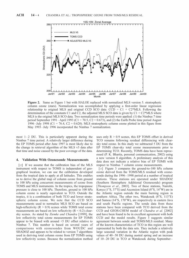
most 1–2 DU. This is particularly apparent during theNimbus 7 time period. A relatively larger difference duringthe EP TOMS period after June 1997 is most likely due tothe change in retrieval algorithm of the MLS v5 data afterthat time and noise caused by the poor coverage of the data.

4. Validation With Ozonesonde Measurements

[12] If we assume that the calibration bias of the MLSinstrument with respect to TOMS is independent of geo-graphical location, we can use the calibration developedfrom the tropical data to apply at all latitudes. This enablesus to derive the global map of column ozone from groundto 100 hPa using concurrent measurements of ozone fromTOMS and MLS instruments. In the tropics, the tropopausepressure is close to 100 hPa. Therefore, ground to 100 hPacolumn ozone is nearly equivalent to TCO. Outside thetropics, it is a combination of both TCO and lower strato-spheric column ozone. We note that the CCD SCOmeasurements used to normalize MLS SCO are based onhigh-reflectivity (R > 0.9) scenes while TOMS total ozonemeasurements are based on low reflectivity (R < 0.2) clear-sky scenes. As stated by Ziemke and Chandra [1999], thelow reflectivity total ozone measurements for EP TOMSappear to be biased with around +5 DU offset relative toNimbus 7. This number is based on several years ofcomparisons with ozonesondes from WOUDC andSHADOZ and appears to be related to version 7 algorithmsused in deriving total column ozone from EP TOMS usinglow reflectivity scenes. Because the normalization method

uses only R > 0.9 scenes, this EP TOMS offset in derivedTCO remains following residual differencing with clear-sky total ozone. In this study we subtracted 5 DU from theEP TOMS clear-sky total ozone measurements prior todetermining TCO. Recently, TOMS data have been reproc-essed (P. K. Bhartia, personal communication, 2002) usinga new version 8 algorithm. A preliminary analysis of thisdata does not indicate a relative bias of EP TOMS withrespect to Nimbus 7 column ozone measurements.[13] Figure 3 compares the ground-to-100 hPa column

ozone derived from the TOMS/MLS residual with ozone-sonde during the 1996–1998 period at a number of tropicalstations. These stations are operated under SHADOZ(Southern Hemisphere Additional Ozonesonde) program[Thompson et al., 2003]. Two of these stations, Nairobi,Kenya (1�S, 37�E) and Ascension Island (8�S, 14�W) are inthe Atlantic region outside the main burning region insouthern Africa. The other two, Watukosek (8�S, 113�E)and Samoa (14�S, 170�W), are respectively in eastern Javaand south Pacific regions. The sonde data from thesestations have been compared with TCO derived from theCCD and GEOS-CHEM model of Chandra et al. [2002]and have been found to be in excellent agreement with bothCCD and the model results. Figure 3 suggests similaragreement between sonde and TOMS/MLS residual. Manyof the known characteristics of TCO in this region are wellrepresented by both the data sets. They include a relativelylarge seasonal variation in the Atlantic region with peakvalues of 40–50 DU during austral spring and an increaseof 10–20 DU in TCO at Watukosek during September–

Figure 2. Same as Figure 1 but with HALOE replaced with normalized MLS version 5. stratosphericcolumn ozone (stars). Normalization was accomplished by applying a first-order linear regressionrelationship to original MLS and original CCD SCO data: CCD = C1 + C2*MLS. Following thedetermination of the constants C1 and C2, the adjusted MLS SCO data is given by C1 + C2*MLS whereMLS is the original MLS SCO data. Two normalization time periods were applied: (1) the Nimbus 7 timeperiod September 1991–April 1993 (C1 = 70.5, C2 = 0.673), and (2) the Earth Probe time period August1996–July 1998 (C1 = 76.4, C2 = 0.620). MLS stratospheric column ozone plotted in this figure fromMay 1993–July 1996 incorporated the Nimbus 7 normalization.


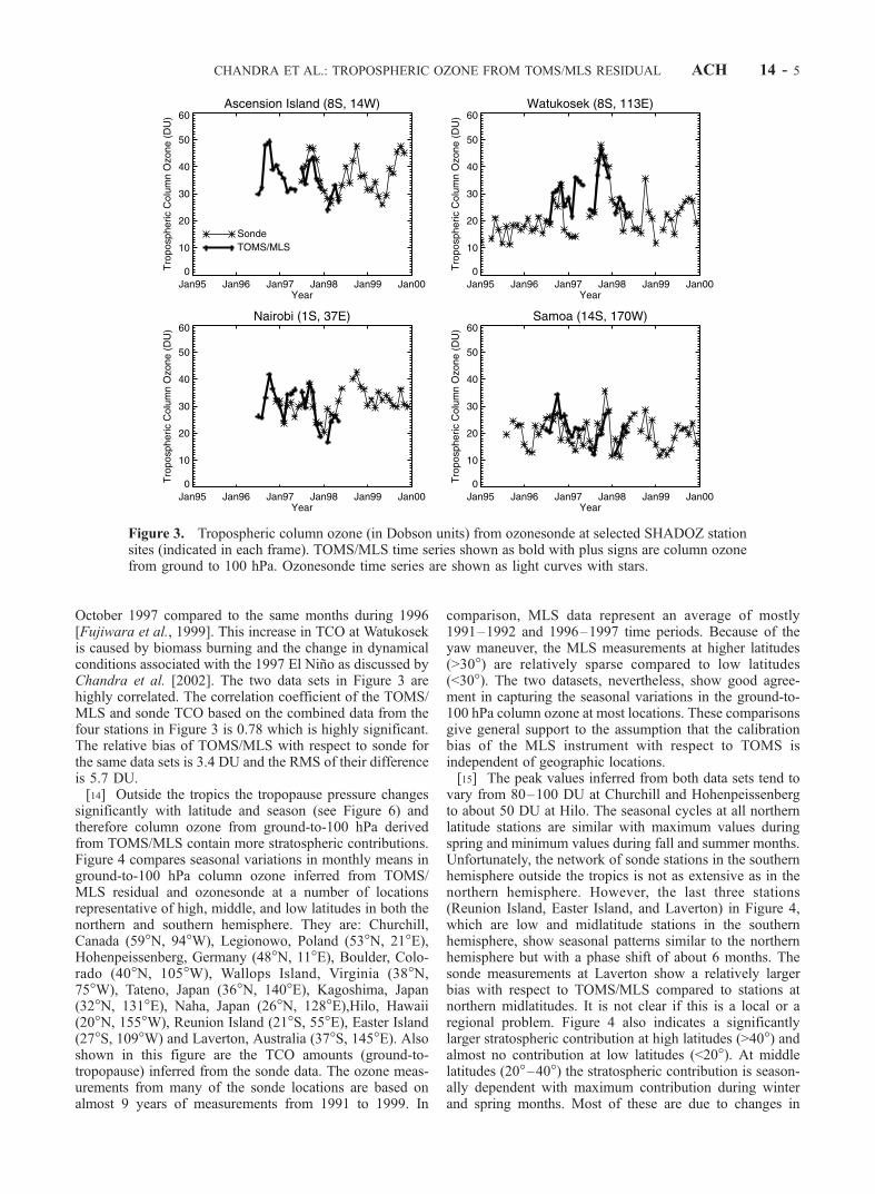
October 1997 compared to the same months during 1996[Fujiwara et al., 1999]. This increase in TCO at Watukosekis caused by biomass burning and the change in dynamicalconditions associated with the 1997 El Nino as discussed byChandra et al. [2002]. The two data sets in Figure 3 arehighly correlated. The correlation coefficient of the TOMS/MLS and sonde TCO based on the combined data from thefour stations in Figure 3 is 0.78 which is highly significant.The relative bias of TOMS/MLS with respect to sonde forthe same data sets is 3.4 DU and the RMS of their differenceis 5.7 DU.[14] Outside the tropics the tropopause pressure changes

significantly with latitude and season (see Figure 6) andtherefore column ozone from ground-to-100 hPa derivedfrom TOMS/MLS contain more stratospheric contributions.Figure 4 compares seasonal variations in monthly means inground-to-100 hPa column ozone inferred from TOMS/MLS residual and ozonesonde at a number of locationsrepresentative of high, middle, and low latitudes in both thenorthern and southern hemisphere. They are: Churchill,Canada (59�N, 94�W), Legionowo, Poland (53�N, 21�E),Hohenpeissenberg, Germany (48�N, 11�E), Boulder, Colo-rado (40�N, 105�W), Wallops Island, Virginia (38�N,75�W), Tateno, Japan (36�N, 140�E), Kagoshima, Japan(32�N, 131�E), Naha, Japan (26�N, 128�E),Hilo, Hawaii(20�N, 155�W), Reunion Island (21�S, 55�E), Easter Island(27�S, 109�W) and Laverton, Australia (37�S, 145�E). Alsoshown in this figure are the TCO amounts (ground-to-tropopause) inferred from the sonde data. The ozone meas-urements from many of the sonde locations are based onalmost 9 years of measurements from 1991 to 1999. In

comparison, MLS data represent an average of mostly1991–1992 and 1996–1997 time periods. Because of theyaw maneuver, the MLS measurements at higher latitudes(>30�) are relatively sparse compared to low latitudes(<30�). The two datasets, nevertheless, show good agree-ment in capturing the seasonal variations in the ground-to-100 hPa column ozone at most locations. These comparisonsgive general support to the assumption that the calibrationbias of the MLS instrument with respect to TOMS isindependent of geographic locations.[15] The peak values inferred from both data sets tend to

vary from 80–100 DU at Churchill and Hohenpeissenbergto about 50 DU at Hilo. The seasonal cycles at all northernlatitude stations are similar with maximum values duringspring and minimum values during fall and summer months.Unfortunately, the network of sonde stations in the southernhemisphere outside the tropics is not as extensive as in thenorthern hemisphere. However, the last three stations(Reunion Island, Easter Island, and Laverton) in Figure 4,which are low and midlatitude stations in the southernhemisphere, show seasonal patterns similar to the northernhemisphere but with a phase shift of about 6 months. Thesonde measurements at Laverton show a relatively largerbias with respect to TOMS/MLS compared to stations atnorthern midlatitudes. It is not clear if this is a local or aregional problem. Figure 4 also indicates a significantlylarger stratospheric contribution at high latitudes (>40�) andalmost no contribution at low latitudes (<20�). At middlelatitudes (20�–40�) the stratospheric contribution is season-ally dependent with maximum contribution during winterand spring months. Most of these are due to changes in

Figure 3. Tropospheric column ozone (in Dobson units) from ozonesonde at selected SHADOZ stationsites (indicated in each frame). TOMS/MLS time series shown as bold with plus signs are column ozonefrom ground to 100 hPa. Ozonesonde time series are shown as light curves with stars.


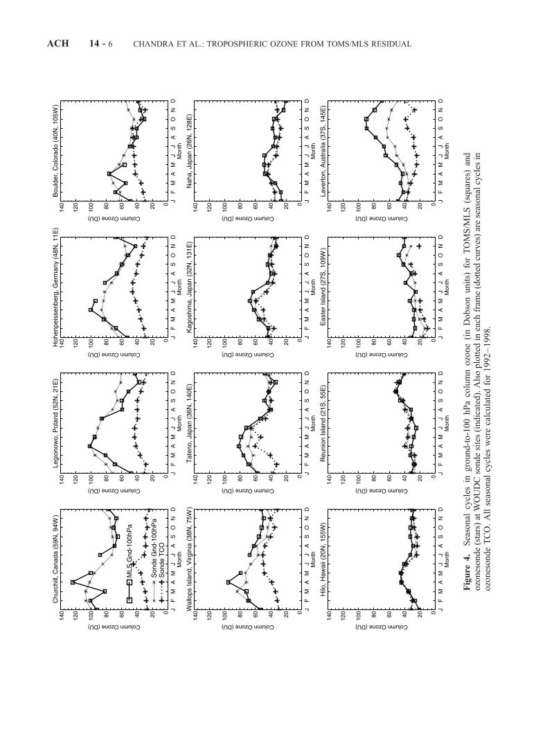
Figure

4.

Seasonal

cycles

inground-to-100hPacolumnozone(inDobsonunits)

forTOMS/M

LS(squares)and

ozonesonde(stars)atWOUDCsondesites(indicated).Alsoplotted

ineach

fram

e(dotted

curves)areseasonalcycles

inozonesondeTCO.Allseasonal

cycles

werecalculatedfor1992–1998.


tropopause height at middle and high latitudes. Table 1gives the relative bias of TOMS/MLS with respect to sondefor the 12 stations in Figure 4. Shown in this table are alsothe root mean square (RMS) values of their difference andtheir correlation coefficient (r). Table 1 shows good corre-lation between TOMS/MLS and sonde data at all locationsexcept Naha. Their relative bias tends to be low (< 4 DU)except for some of the higher-latitude stations, e.g., Legio-nowo, Boulder, and Laverton.

5. High-Resolution Global Maps

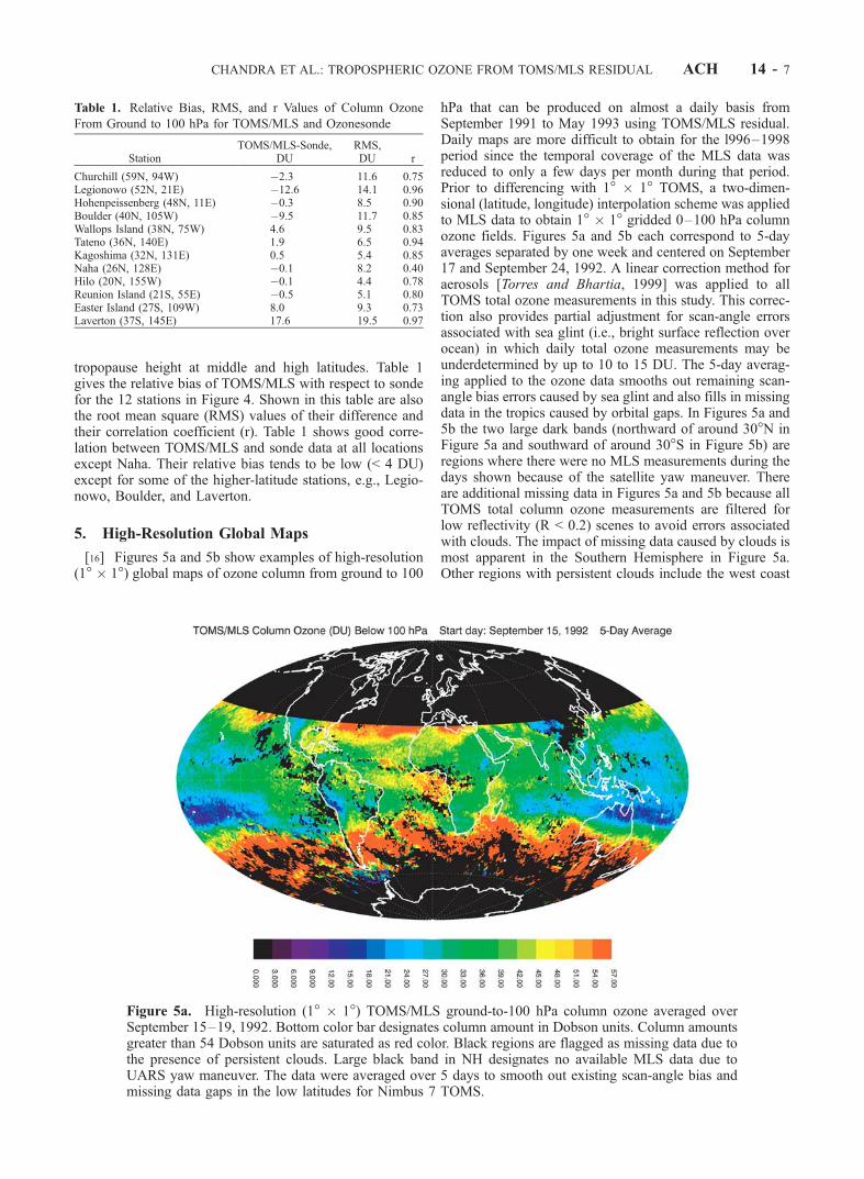
[16] Figures 5a and 5b show examples of high-resolution(1� � 1�) global maps of ozone column from ground to 100

hPa that can be produced on almost a daily basis fromSeptember 1991 to May 1993 using TOMS/MLS residual.Daily maps are more difficult to obtain for the l996–1998period since the temporal coverage of the MLS data wasreduced to only a few days per month during that period.Prior to differencing with 1� � 1� TOMS, a two-dimen-sional (latitude, longitude) interpolation scheme was appliedto MLS data to obtain 1� � 1� gridded 0–100 hPa columnozone fields. Figures 5a and 5b each correspond to 5-dayaverages separated by one week and centered on September17 and September 24, 1992. A linear correction method foraerosols [Torres and Bhartia, 1999] was applied to allTOMS total ozone measurements in this study. This correc-tion also provides partial adjustment for scan-angle errorsassociated with sea glint (i.e., bright surface reflection overocean) in which daily total ozone measurements may beunderdetermined by up to 10 to 15 DU. The 5-day averag-ing applied to the ozone data smooths out remaining scan-angle bias errors caused by sea glint and also fills in missingdata in the tropics caused by orbital gaps. In Figures 5a and5b the two large dark bands (northward of around 30�N inFigure 5a and southward of around 30�S in Figure 5b) areregions where there were no MLS measurements during thedays shown because of the satellite yaw maneuver. Thereare additional missing data in Figures 5a and 5b because allTOMS total column ozone measurements are filtered forlow reflectivity (R < 0.2) scenes to avoid errors associatedwith clouds. The impact of missing data caused by clouds ismost apparent in the Southern Hemisphere in Figure 5a.Other regions with persistent clouds include the west coast

Table 1. Relative Bias, RMS, and r Values of Column Ozone

From Ground to 100 hPa for TOMS/MLS and Ozonesonde

StationTOMS/MLS-Sonde,

DURMS,DU r

Churchill (59N, 94W) �2.3 11.6 0.75Legionowo (52N, 21E) �12.6 14.1 0.96Hohenpeissenberg (48N, 11E) �0.3 8.5 0.90Boulder (40N, 105W) �9.5 11.7 0.85Wallops Island (38N, 75W) 4.6 9.5 0.83Tateno (36N, 140E) 1.9 6.5 0.94Kagoshima (32N, 131E) 0.5 5.4 0.85Naha (26N, 128E) �0.1 8.2 0.40Hilo (20N, 155W) �0.1 4.4 0.78Reunion Island (21S, 55E) �0.5 5.1 0.80Easter Island (27S, 109W) 8.0 9.3 0.73Laverton (37S, 145E) 17.6 19.5 0.97

Figure 5a. High-resolution (1� � 1�) TOMS/MLS ground-to-100 hPa column ozone averaged overSeptember 15–19, 1992. Bottom color bar designates column amount in Dobson units. Column amountsgreater than 54 Dobson units are saturated as red color. Black regions are flagged as missing data due tothe presence of persistent clouds. Large black band in NH designates no available MLS data due toUARS yaw maneuver. The data were averaged over 5 days to smooth out existing scan-angle bias andmissing data gaps in the low latitudes for Nimbus 7 TOMS.


of South America and Central America, the equatorialAtlantic, and eastern Asia.[17] Despite limitations of the combined TOMS and MLS

measurements, Figures 5a and 5b highlight numerousdetails regarding both ozone properties and the meteoro-logical conditions present. The changes in tropopausepressure are most pronounced in regions associated withthe upper tropospheric wind jets. At midlatitudes, the windjets can be identified from color gradients that change fromgreen (�40 DU) to yellow (�50 DU) to orange (> 50 DU).The wind jet regions are more easily identified in theSouthern Hemisphere and appear as the boundary of themeandering orange wave pattern in Figure 5a. Poleward ofthe wind jets the tropopause pressure increases rapidly.[18] The two maps in Figures 5a and 5b essentially show

both the spatial and temporal changes in TCO between ±30�where the tropopause is close 100 hPa. They show well-known features of elevated ozone (40–50 DU) in the tropicsencompassing the regions between South America andsouthern Africa [e.g., Chandra et al., 2002]. The tropicalenhancement during this time is usually attributed to bio-mass burning in southern Africa and Brazil. However, theelevated ozone occurs over most of the Atlantic Oceansouth of the equator and not over land where the biomassburning takes place. Ozone is also elevated over regionsnorth and south of 30� latitude. Most of this increase may beattributed to increased stratospheric contribution as indi-cated in Figure 4.[19] Figures 5a and 5b depict several other features such

as persistent low ozone over mountainous regions such asAndes and Himalayas (down to values less than 10 DU).Low ozone values in these regions are topographicallyinduced. The high ozone in the Atlantic exhibits a plumestretching toward South America as observed during the

TRACE-A experiment [Fishman et al., 1996]. Also largeramounts occur for September 15–19 when compared toSeptember 22–26. The rapid loss of ozone over only oneweek time period in the Atlantic suggests that much of theozone may have been in the low to middle tropospherewhere rapid ozone destruction occurs [Jacob et al., 1996;Thompson et al., 1996].

6. Tropospheric Column Ozone (TCO) FromTOMS/MLS Residual

[20] In order to calculate TCO from TOMS/MLS resid-ual, it is necessary to account for the excess ozone �O3

between the tropopause and 100 hPa. Over most of thetropical latitudes this is not a problem since the tropopauseis close to 100 hPa. The tropopause does not deviatesignificantly from 100 hPa over latitudes between ±30�and a simple correction can be made for �O3. Figure 6shows a climatology of zonal mean tropopause pressure(TP) derived from seven years (1992–1998) of NationalCenters for Environmental Prediction (NCEP) temperatureprofiles, using the World Meteorological Organizationcriterion [e.g., Logan, 1999, and references therein] ofdetermining tropopause. According to this criterion thetropopause is defined as the lowest level at which thetemperature lapse rate decreases to 2K/km or less providedthe average lapse rate between this level and all higherlevels within the next 2 km does not exceed 2K/km. Thetropopause calculated from the WMO definition does notdiffer significantly from the cold-point tropopause defini-tion over most of the tropical and low latitudes, but theWMO tropopause pressure can be up to 40 hPa greaterthan the cold-point tropopause pressure near 30�N. Thelatter is defined as the pressure at which temperature

Figure 5b. Same as Figure 5a but for September 22–26, 1992.


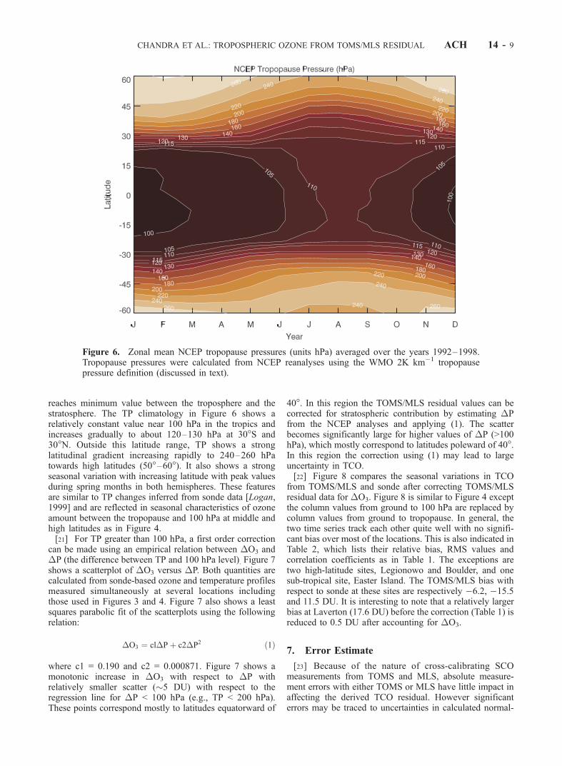
reaches minimum value between the troposphere and thestratosphere. The TP climatology in Figure 6 shows arelatively constant value near 100 hPa in the tropics andincreases gradually to about 120–130 hPa at 30�S and30�N. Outside this latitude range, TP shows a stronglatitudinal gradient increasing rapidly to 240–260 hPatowards high latitudes (50�–60�). It also shows a strongseasonal variation with increasing latitude with peak valuesduring spring months in both hemispheres. These featuresare similar to TP changes inferred from sonde data [Logan,1999] and are reflected in seasonal characteristics of ozoneamount between the tropopause and 100 hPa at middle andhigh latitudes as in Figure 4.[21] For TP greater than 100 hPa, a first order correction

can be made using an empirical relation between �O3 and�P (the difference between TP and 100 hPa level). Figure 7shows a scatterplot of �O3 versus �P. Both quantities arecalculated from sonde-based ozone and temperature profilesmeasured simultaneously at several locations includingthose used in Figures 3 and 4. Figure 7 also shows a leastsquares parabolic fit of the scatterplots using the followingrelation:

�O3 ¼ cl�Pþ c2�P2 ð1Þ

where c1 = 0.190 and c2 = 0.000871. Figure 7 shows amonotonic increase in �O3 with respect to �P withrelatively smaller scatter (�5 DU) with respect to theregression line for �P < 100 hPa (e.g., TP < 200 hPa).These points correspond mostly to latitudes equatorward of

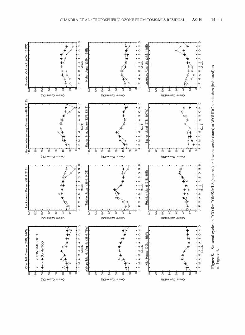
40�. In this region the TOMS/MLS residual values can becorrected for stratospheric contribution by estimating �Pfrom the NCEP analyses and applying (1). The scatterbecomes significantly large for higher values of �P (>100hPa), which mostly correspond to latitudes poleward of 40�.In this region the correction using (1) may lead to largeuncertainty in TCO.[22] Figure 8 compares the seasonal variations in TCO

from TOMS/MLS and sonde after correcting TOMS/MLSresidual data for �O3. Figure 8 is similar to Figure 4 exceptthe column values from ground to 100 hPa are replaced bycolumn values from ground to tropopause. In general, thetwo time series track each other quite well with no signifi-cant bias over most of the locations. This is also indicated inTable 2, which lists their relative bias, RMS values andcorrelation coefficients as in Table 1. The exceptions aretwo high-latitude sites, Legionowo and Boulder, and onesub-tropical site, Easter Island. The TOMS/MLS bias withrespect to sonde at these sites are respectively �6.2, �15.5and 11.5 DU. It is interesting to note that a relatively largerbias at Laverton (17.6 DU) before the correction (Table 1) isreduced to 0.5 DU after accounting for �O3.

7. Error Estimate

[23] Because of the nature of cross-calibrating SCOmeasurements from TOMS and MLS, absolute measure-ment errors with either TOMS or MLS have little impact inaffecting the derived TCO residual. However significanterrors may be traced to uncertainties in calculated normal-

Figure 6. Zonal mean NCEP tropopause pressures (units hPa) averaged over the years 1992–1998.Tropopause pressures were calculated from NCEP reanalyses using the WMO 2K km�1 tropopausepressure definition (discussed in text).


ization coefficients. Another source of error in TCO is theozonesonde regression adjustment (Figure 7) made fortropopause pressures deviating from 100 hPa at latitudesbetween ±30�. While it is possible to quantify all of theseerrors from statistical uncertainties in the regression coef-ficients, we have opted instead to compare the final derivedvalues of TOMS/MLS ground-to-100 hPa column ozonewith similar measurements from ozonesondes by calculating2s differences (s being one standard deviation) assumingozonesonde data as truth. Because the tropopause is con-sistently around 100–110 hPa year-round in the tropics, theground-to-100 hPa column amount in the tropics is equiv-alent to TCO within 1–2 DU.[24] The TCO validation in this study involved compar-

isons of both 1998 tropical SHADOZ and pre-SHADOZ(prior to 1998) WOUDC tropical and extratropical ozone-sonde measurements. Because Nimbus 7 and EP TOMSdata are from different time periods, separate regressioncalibrations/normalizations were invoked. The SHADOZand WOUDC ozonesonde data were compared independ-ently with TOMS/MLS TCO for the Nimbus 7 and EPTOMS time periods. Also, independent tropical and extra-tropical (extending to ±40� latitude) comparisons weremade for both Nimbus 7 and EP TOMS. For the tropics,WOUDC ozonesonde data from Ascension Island (8S,14W) and Brazzaville (4S, 15E) for the Nimbus 7 timeperiod were available for comparison during September1991–October 1992 and indicated an average 2s error of

3.5 DU. In the tropics, 11 stations sites for SHADOZ andWOUDC ozonesondes (including the SHADOZ sites plot-ted in Figure 3) for August 1996 through 1998 indicated anaverage 2s value of 4 DU for the EP TOMS time period.For the extratropics extending to ±40� latitude (i.e., encom-passing the subtropics in both hemispheres), ground-to-100hPa column ozone for both Nimbus 7 and Earth Probe timeperiods were compared with similar measurements fromWOUDC ozonesondes at 7 station sites.[25] For the Nimbus 7 time period, ground-to-100 hPa

column ozone up to latitudes ±40� showed an average 2svalue of 6 DU. For the EP TOMS time period an average 2serror of 8 DU was indicated. When WOUDC data wereextended only to ±35� latitudes the 2s values for bothNimbus7 and EP TOMS were around 5 DU. In this study we analyzeonly TCO data equatorward of ±30� latitude. In summary,ozonesonde comparisons indicate that an estimate for 2suncertainty in local TCO measurements for either Nimbus 7or EP TOMS time periods is 5 DU for these latitudes.

8. Zonal Variability in TCO and SCO

[26] One of the basic assumptions in deriving TCO fromthe CCD method was to assume that SCO estimated fromhigh reflecting clouds in the Pacific was zonally invariantwithin 5 DU over all tropical latitudes. This assumption wasbased on stratospheric ozone data from SAGE [Fishman etal., 1990; Shiotani and Hasebe, 1994], MLS [Ziemke et al.,

Figure 7. Scatterplot of column ozone between tropopause and 100 hPa (�O3) versus the difference oftropopause pressure minus 100 hPa (�P). Both �O3 along vertical axis (in Dobson units) and �P alonghorizontal axis (in hPa) were calculated from sonde-based ozone and temperature profiles measuredsimultaneously at the locations shown in Figures 5a and 5b. The tropopause pressure was calculated fromtemperature profiles using the cold point definition. Also shown in this figure is a least squares parabolicfit of the scatterplot using the regression relation �O3 = C1 � �P + C2 � �P2 where C1 = 0.190 and C2 =0.000871. The statistical 2s value for C1 is 0.0367 and for C2 it is 0.000222 (see text for discussion ofregression method).


Figure

8.

Seasonalcycles

inTCOforTOMS/M

LS(squares)andozonesonde(stars)atWOUDCsondesites(indicated)as

inFigure

4.


1996], and MLS and HALOE [Ziemke et al., 1998]. Morerecently the zonal invariance of SCO in the tropics wascorroborated from ozonesonde measurements from SHA-DOZ [Thompson et al., 2003]. Figures 9a and 9b (lowerpanels) suggest that SCO is zonally invariant within this

range not only in the tropics but also to within 10 DUoutside the tropics extending to about 30� latitude in bothhemispheres. These figures also compare zonal variability inTCO derived from the CCD method assuming a zonallyinvariant stratosphere (upper panels) with TCO derivedfrom the TOMS/MLS residual. The latter implicitlyaccounts for the zonal variability in SCO. Figures 9a and9b are based on September 1991 and February 1997 data.They suggest that the zonal characteristics of TCO derivedfrom the CCD method are similar to those derived from theTOMS/MLS residual method within the uncertainty of thezonal variability of SCO. In the latitude region between10�N and 10�S, the zonal correlation of TOMS/MLS andCCD for September 1991 is 0.9, their relative bias (TOMS/MLS-CCD) is �1.9 DU and the RMS of their difference is4.1 DU. For February 1997, the corresponding values arerespectively 0.94, �0.8 DU and 2.1 DU.[27] Both Figures 9a and 9b show a predominant wave

one feature in the tropics with maximum values in theAtlantic and minimum values in the Pacific. Outside thetropics, the wave one features in the troposphere weaken

Table 2. Same as Table 1 Except for Column Ozone From

Ground to Tropopause (TCO)

StationTOMS/MLS-Sonde,

DURMS,DU r

Churchill (59N, 94W) 0.0 9.5 0.30Legionowo (52N, 21E) �6.2 11.1 0.85Hohenpeissenberg (48N, 11E) �2.4 10.8 0.70Boulder (40N, 105W) �15.5 15.9 0.85Wallops Island (38N, 75W) �3.0 7.4 0.81Tateno (36N, 140E) �5.9 9.3 0.87Kagoshima (32N, 131E) �4.2 7.4 0.76Naha (26N, 128E) �2.6 8.4 0.43Hilo (20N, 155W) �1.7 4.6 0.79Reunion Island (21S, 55E) �3.0 6.2 0.77Easter Island (27S, 109W) 11.5 11.3 0.64Laverton (37S, 145E) �0.5 13.2 0.72

Figure 9a. Top: Monthly mean CCD TCO for September, 1991. Middle: Monthly mean TOMS/MLSTCO for September 1991. Bottom: Monthly mean MLS SCO for September 1991.


considerably. The decline of the wave 1 pattern outside thetropics is associated with a decline in lightning activity andWalker circulation as indicated from the GEOS-CHEMmodel (section 9).[28] The zonal characteristics of SCO, inferred from

Figures 9a and 9b, are typical of the entire data sets basedon TOMS/MLS residual including the El Nino years. Eventhough they show significant latitudinal and seasonal vari-ability, their zonal variability is generally less than 5 DU attropical and sub-tropical latitudes with no specific zonalpattern. They do not support the conclusions of Newchurchet al. [2001] about the presence of a wave one in SCO withabout 8–10 DU increase from the Pacific to the Atlanticregion. The conclusions by Newchurch et al. [2001] werebased on data from Nimbus 7 TOMS and the Nimbus 7Temperature Humidity Infrared (THIR) sensor. Theseauthors questioned the conclusions based on MLS, HALOEand SAGE data because of profile measurement uncertain-ties from these instruments below 68 hPa and the poorspatial sampling of the observational data from limb scan-ning satellite instruments of HALOE and SAGE. Thesearguments do not seem to be valid, since SCO is a column

integral from 100 hPa to the top of the atmosphere and thecontribution to SCO from the region between 68–100 hPais only about 2–3 percent (�6–8 DU) [Ziemke et al., 1996].It is not likely to introduce an error in the column amountsignificant enough to produce a an 8–10 DU peak-to-peakzonal wave 1 in SCO. In addition, RMS uncertainties inSCO as shown by Newchurch et al. [2001] are as large asthe measurements of derived SCO, and the data samplingfrom the technique is unfortunately limited in the tropics, asmuch if not more limited than either SAGE or HALOEoccultation measurements. Current investigation of theTOMS/THIR method (M. Newchurch and Z. Ahmad,personal communication, 2002) suggests that the increasesin SCO over the Atlantic (mostly observed increases overSouth America and African land masses shown by New-church et al. [2001]) may be attributed to multiple-scatter-ing of UV within highly reflecting convective clouds(reflectivity R > 0.8) in the presence of large ozone contentin the upper troposphere within the cloud tops. Thisscattering does not appear to affect the CCD measurementsof Ziemke et al. [1998] since SCO is determined over thePacific where ozone content in the upper troposphere is

Figure 9b. Same as Figure 9a but for February 1997.


generally small compared to the Atlantic region [Kley et al.,1996].

9. Comparison With the GEOS-CHEM Model

[29] As discussed by Chandra et al. [2002] and Martin etal. [2002] and noted earlier in the introduction, the zonaland seasonal characteristics of TCO derived from the CCDmethod during the 1996–1997 period are well representedby the GEOS-CHEM model at tropical latitudes south of theequator. The agreement, however, breaks down north of theequator over sub-Saharan northern Africa where the sea-sonal variations in model and observation tend to be out ofphase. The TCO data obtained from TOMS/MLS allows thecomparison of GEOS-CHEM model well outside the tropicswhere sonde data can be used for cross validation. In thefollowing, we will make some of these comparisons anddiscuss their implications.[30] The GEOS-CHEM model was initially described by

Bey et al. [2001a]. Subsequent improvements are describedby Martin et al. [2002]. The model is driven by assimilatedmeteorological data updated every 3–6 hours from theGlobal Earth Observing System (GEOS) of the NASA DataAssimilation Office (DAO) [Schubert et al., 1993]. We usefor this study the GEOS data for 1996–97, available with aresolution of 2� latitude by 2.5� longitude and 46 sigmalevels in the vertical extending up to 0.1 hPa. For computa-tional expedience we degrade the horizontal resolution to 4�latitude by 5� longitude and merge the vertical levels abovethe lower stratosphere, retaining a total of 26. We conductsimulations from March 1996 through November 1997. Thefirst six months are used to achieve proper initialization. Wepresent results for September 1996 through November 1997.[31] The GEOS-CHEMmodel includes a detailed descrip-

tion of tropospheric O3-NOx-hydrocarbon chemistry. It sol-ves the chemical evolution of about 120 species with a Gear

solver [Jacobson and Turco, 1994] and transports 24 tracers.Photolysis frequencies are computed using the Fast-J radi-ative transfer algorithm [Wild et al., 2000], which includesRayleigh scattering as well as Mie scattering by clouds andmineral dust. The tropopause in the model is determinedusing the World Meteorological Organization standard crite-rion of a 2 K km�1 lapse rate. The cross-tropopause transportof ozone is simulated by the Synoz (synthetic ozone) method[McLinden et al., 2000] using their recommended flux of475 Tg O3 yr

�1.[32] Emissions of NOx from lightning are 6 Tg N yr�1

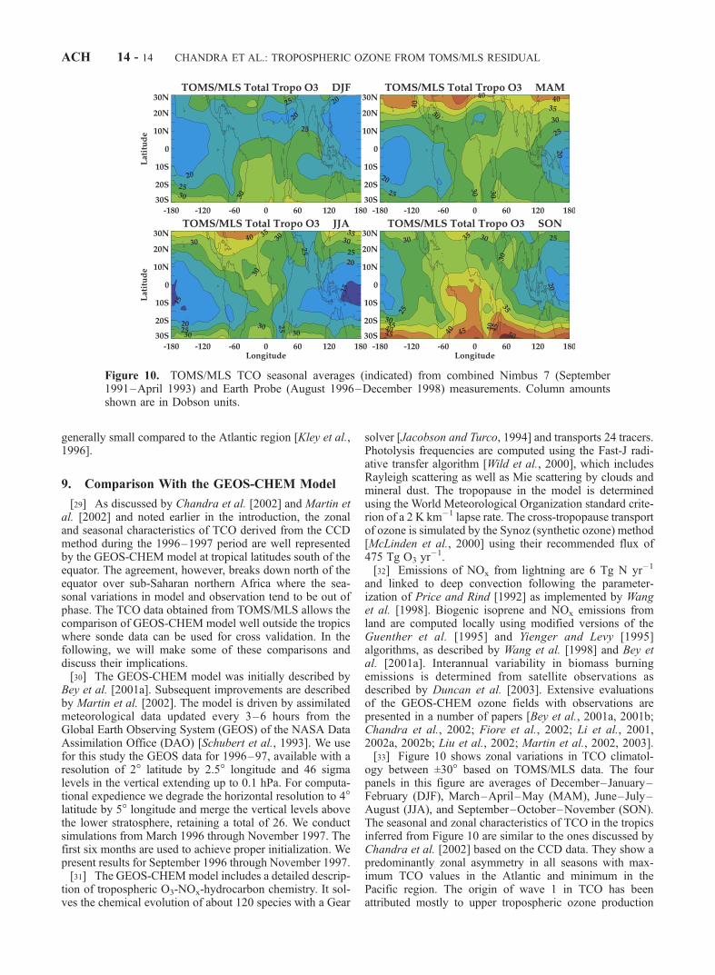
and linked to deep convection following the parameter-ization of Price and Rind [1992] as implemented by Wanget al. [1998]. Biogenic isoprene and NOx emissions fromland are computed locally using modified versions of theGuenther et al. [1995] and Yienger and Levy [1995]algorithms, as described by Wang et al. [1998] and Bey etal. [2001a]. Interannual variability in biomass burningemissions is determined from satellite observations asdescribed by Duncan et al. [2003]. Extensive evaluationsof the GEOS-CHEM ozone fields with observations arepresented in a number of papers [Bey et al., 2001a, 2001b;Chandra et al., 2002; Fiore et al., 2002; Li et al., 2001,2002a, 2002b; Liu et al., 2002; Martin et al., 2002, 2003].[33] Figure 10 shows zonal variations in TCO climatol-

ogy between ±30� based on TOMS/MLS data. The fourpanels in this figure are averages of December–January–February (DJF), March–April–May (MAM), June–July–August (JJA), and September–October–November (SON).The seasonal and zonal characteristics of TCO in the tropicsinferred from Figure 10 are similar to the ones discussed byChandra et al. [2002] based on the CCD data. They show apredominantly zonal asymmetry in all seasons with max-imum TCO values in the Atlantic and minimum in thePacific region. The origin of wave 1 in TCO has beenattributed mostly to upper tropospheric ozone production

Figure 10. TOMS/MLS TCO seasonal averages (indicated) from combined Nimbus 7 (September1991–April 1993) and Earth Probe (August 1996–December 1998) measurements. Column amountsshown are in Dobson units.


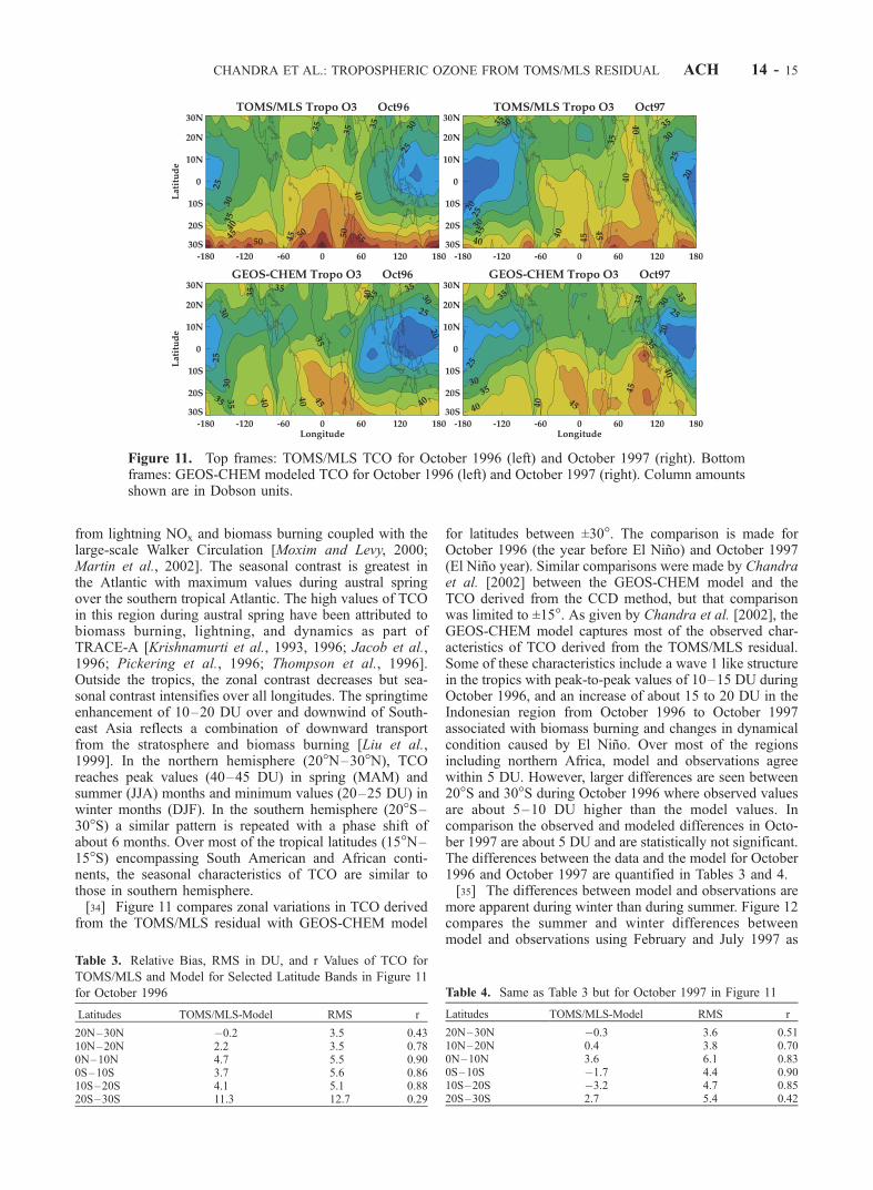
from lightning NOx and biomass burning coupled with thelarge-scale Walker Circulation [Moxim and Levy, 2000;Martin et al., 2002]. The seasonal contrast is greatest inthe Atlantic with maximum values during austral springover the southern tropical Atlantic. The high values of TCOin this region during austral spring have been attributed tobiomass burning, lightning, and dynamics as part ofTRACE-A [Krishnamurti et al., 1993, 1996; Jacob et al.,1996; Pickering et al., 1996; Thompson et al., 1996].Outside the tropics, the zonal contrast decreases but sea-sonal contrast intensifies over all longitudes. The springtimeenhancement of 10–20 DU over and downwind of South-east Asia reflects a combination of downward transportfrom the stratosphere and biomass burning [Liu et al.,1999]. In the northern hemisphere (20�N–30�N), TCOreaches peak values (40–45 DU) in spring (MAM) andsummer (JJA) months and minimum values (20–25 DU) inwinter months (DJF). In the southern hemisphere (20�S–30�S) a similar pattern is repeated with a phase shift ofabout 6 months. Over most of the tropical latitudes (15�N–15�S) encompassing South American and African conti-nents, the seasonal characteristics of TCO are similar tothose in southern hemisphere.[34] Figure 11 compares zonal variations in TCO derived

from the TOMS/MLS residual with GEOS-CHEM model

for latitudes between ±30�. The comparison is made forOctober 1996 (the year before El Nino) and October 1997(El Nino year). Similar comparisons were made by Chandraet al. [2002] between the GEOS-CHEM model and theTCO derived from the CCD method, but that comparisonwas limited to ±15�. As given by Chandra et al. [2002], theGEOS-CHEM model captures most of the observed char-acteristics of TCO derived from the TOMS/MLS residual.Some of these characteristics include a wave 1 like structurein the tropics with peak-to-peak values of 10–15 DU duringOctober 1996, and an increase of about 15 to 20 DU in theIndonesian region from October 1996 to October 1997associated with biomass burning and changes in dynamicalcondition caused by El Nino. Over most of the regionsincluding northern Africa, model and observations agreewithin 5 DU. However, larger differences are seen between20�S and 30�S during October 1996 where observed valuesare about 5–10 DU higher than the model values. Incomparison the observed and modeled differences in Octo-ber 1997 are about 5 DU and are statistically not significant.The differences between the data and the model for October1996 and October 1997 are quantified in Tables 3 and 4.[35] The differences between model and observations are

more apparent during winter than during summer. Figure 12compares the summer and winter differences betweenmodel and observations using February and July 1997 as

Figure 11. Top frames: TOMS/MLS TCO for October 1996 (left) and October 1997 (right). Bottomframes: GEOS-CHEM modeled TCO for October 1996 (left) and October 1997 (right). Column amountsshown are in Dobson units.

Table 3. Relative Bias, RMS in DU, and r Values of TCO for

TOMS/MLS and Model for Selected Latitude Bands in Figure 11

for October 1996

Latitudes TOMS/MLS-Model RMS r

20N–30N �0.2 3.5 0.4310N–20N 2.2 3.5 0.780N–10N 4.7 5.5 0.900S–10S 3.7 5.6 0.8610S–20S 4.1 5.1 0.8820S–30S 11.3 12.7 0.29

Table 4. Same as Table 3 but for October 1997 in Figure 11


20N–30N �0.3 3.6 0.5110N–20N 0.4 3.8 0.700N–10N 3.6 6.1 0.830S–10S �1.7 4.4 0.9010S–20S �3.2 4.7 0.8520S–30S 2.7 5.4 0.42


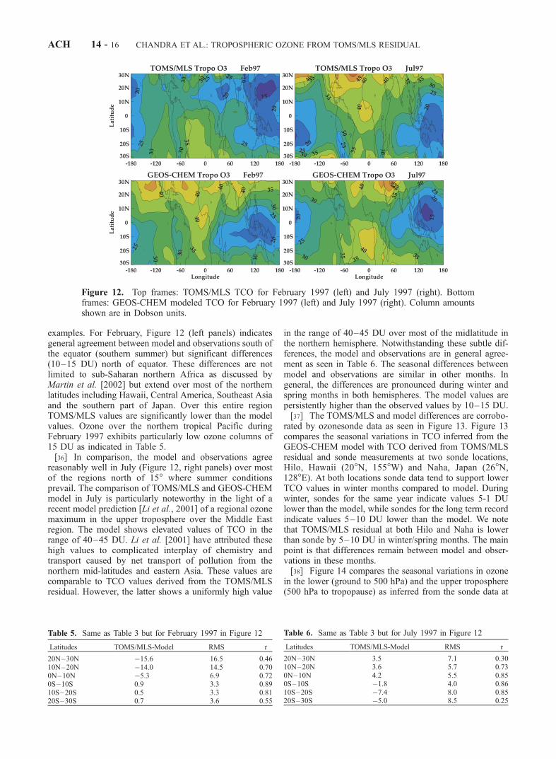
examples. For February, Figure 12 (left panels) indicatesgeneral agreement between model and observations south ofthe equator (southern summer) but significant differences(10–15 DU) north of equator. These differences are notlimited to sub-Saharan northern Africa as discussed byMartin et al. [2002] but extend over most of the northernlatitudes including Hawaii, Central America, Southeast Asiaand the southern part of Japan. Over this entire regionTOMS/MLS values are significantly lower than the modelvalues. Ozone over the northern tropical Pacific duringFebruary 1997 exhibits particularly low ozone columns of15 DU as indicated in Table 5.[36] In comparison, the model and observations agree

reasonably well in July (Figure 12, right panels) over mostof the regions north of 15� where summer conditionsprevail. The comparison of TOMS/MLS and GEOS-CHEMmodel in July is particularly noteworthy in the light of arecent model prediction [Li et al., 2001] of a regional ozonemaximum in the upper troposphere over the Middle Eastregion. The model shows elevated values of TCO in therange of 40–45 DU. Li et al. [2001] have attributed thesehigh values to complicated interplay of chemistry andtransport caused by net transport of pollution from thenorthern mid-latitudes and eastern Asia. These values arecomparable to TCO values derived from the TOMS/MLSresidual. However, the latter shows a uniformly high value

in the range of 40–45 DU over most of the midlatitude inthe northern hemisphere. Notwithstanding these subtle dif-ferences, the model and observations are in general agree-ment as seen in Table 6. The seasonal differences betweenmodel and observations are similar in other months. Ingeneral, the differences are pronounced during winter andspring months in both hemispheres. The model values arepersistently higher than the observed values by 10–15 DU.[37] The TOMS/MLS and model differences are corrobo-

rated by ozonesonde data as seen in Figure 13. Figure 13compares the seasonal variations in TCO inferred from theGEOS-CHEM model with TCO derived from TOMS/MLSresidual and sonde measurements at two sonde locations,Hilo, Hawaii (20�N, 155�W) and Naha, Japan (26�N,128�E). At both locations sonde data tend to support lowerTCO values in winter months compared to model. Duringwinter, sondes for the same year indicate values 5-1 DUlower than the model, while sondes for the long term recordindicate values 5–10 DU lower than the model. We notethat TOMS/MLS residual at both Hilo and Naha is lowerthan sonde by 5–10 DU in winter/spring months. The mainpoint is that differences remain between model and obser-vations in these months.[38] Figure 14 compares the seasonal variations in ozone

in the lower (ground to 500 hPa) and the upper troposphere(500 hPa to tropopause) as inferred from the sonde data at

Figure 12. Top frames: TOMS/MLS TCO for February 1997 (left) and July 1997 (right). Bottomframes: GEOS-CHEM modeled TCO for February 1997 (left) and July 1997 (right). Column amountsshown are in Dobson units.

Table 5. Same as Table 3 but for February 1997 in Figure 12


20N–30N �15.6 16.5 0.4610N–20N �14.0 14.5 0.700N–10N �5.3 6.9 0.720S�10S 0.9 3.3 0.8910S–20S 0.5 3.3 0.8120S–30S 0.7 3.6 0.55

Table 6. Same as Table 3 but for July 1997 in Figure 12


20N–30N 3.5 7.1 0.3010N–20N 3.6 5.7 0.730N–10N 4.2 5.5 0.850S–10S �1.8 4.0 0.8610S–20S �7.4 8.0 0.8520S–30S �5.0 8.5 0.25


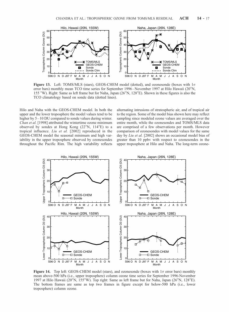
Hilo and Naha with the GEOS-CHEM model. In both theupper and the lower troposphere the model values tend to behigher by 5–10 DU compared to sonde values during winter.Chan et al. [1998] attributed the wintertime ozone minimumobserved by sondes at Hong Kong (22�N, 114�E) to atropical influence. Liu et al. [2002] reproduced in theGEOS-CHEM model the seasonal minimum and high var-iability in the upper troposphere observed by ozonesondesthroughout the Pacific Rim. The high variability reflects

alternating intrusions of stratospheric air, and of tropical airto the region. Some of the model bias shown here may reflectsampling since modeled ozone values are averaged over theentire month, while the ozonesondes and TOMS/MLS dataare comprised of a few observations per month. Howevercomparison of ozonesondes with model values for the sameday by Liu et al. [2002] shows an occasional model bias ofgreater than 10 ppbv with respect to ozonesondes in theupper troposphere at Hilo and Naha. The long-term ozone-

Figure 13. Left: TOMS/MLS (stars), GEOS-CHEM model (dotted), and ozonesonde (boxes with 1serror bars) monthly mean TCO time series for September 1996–November 1997 at Hilo Hawaii (20�N,155 �W). Right: Same as left frame but for Naha, Japan (26�N, 128�E). Shown in these figures is also theTCO climatology based on sonde data (dotted lines).

Figure 14. Top left: GEOS-CHEM model (stars), and ozonesonde (boxes with 1s error bars) monthlymean above-500 hPa (i.e., upper troposphere) column ozone time series for September 1996-November1997 at Hilo Hawaii (20�N, 155�W). Top right: Same as left frame but for Naha, Japan (26�N, 128�E).The bottom frames are same as top two frames in figure except for below-500 hPa (i.e., lowertroposphere) column ozone.


sonde record (Figure 13) suggests a similar model bias.Models also have difficulty in reproducing aircraft observa-tions of less than 30 ppbv in the lower troposphere over thenorthern Tropical Pacific [Staudt et al., 2002].

10. Summary and Conclusions

[39] In this paper, we have derived daily and monthlymaps of TCO at tropical and middle latitudes based on theTOR principle, which uses concurrent measurements oftotal column ozone from the TOMS (version 7) instrumentand SCO from the MLS (version 5) instrument on UARS.The key to the success of this method is calibration of theMLS SCO data to be compatible with TOMS measure-ments. This is achieved by applying CCD derived SCOmeasurements as a transfer standard. Because the MLSozone measurements are limited to regions above 100 hPa,TOMS/MLS residual, in principle, is capable of producingglobal maps of column ozone from ground-to-100 km.Comparison with ozonesonde data suggests that at lati-tudes greater than 30�, TOMS/MLS residual has a sig-nificant contribution from the stratosphere, which increasesrapidly towards higher latitude with the increase of tropo-pause pressure. The stratospheric contribution has a strongseasonal dependence with maximum contribution duringspring months when tropopause pressure is higher than100 hPa. Over most of the regions between 30�S and30�N the tropopause pressure is close to 100 hPa and theTOMS/MLS residual can be used to generate TCO mapswith only a minor adjustment for tropopause pressure.[40] Our study has shown that the zonal variability in

TOMS total column ozone at tropical and subtropicallatitudes is mostly of tropospheric origin. The zonal contrastin TCO maximizes near the equator and weakens consid-erably outside the tropics. The tropical zonal contrast isusually characterized by wave 1 except during the 1997–1998 El Nino when TCO was significantly elevated forseveral months in 1997 over half the tropical belt encom-passing South America, Southern Africa and Indonesia. Theseasonal and zonal variability in TCO in the tropics, derivedfrom the TOMS/MLS residual, are consistent with thosederived from the CCD method and ozonesonde data bothfor El Nino and non-El Nino years.[41] A comparison of TCO derived from the TOMS/MLS

residual and GEOS-CHEM model for the 1996–1997period shows good agreement in the tropics south of theequator consistent with the previous studies [Chandra et al.,2002]. Both the model and observations show similar zonaland seasonal characteristics including the enhancement ofTCO in the Indonesian region associated with El Nino in1997, and the poleward decline of the wave-1 patternassociated with the decline of lightning activity and thelarge-scale Walker Circulation. The model and observatio-nal differences increase with latitude during winter andspring.[42] The methodology for deriving TCO using TOMS/

MLS residual is limited to ±30� in latitudes because theMLS instrument on UARS cannot measure ozone below100 hPa. This restriction should not apply to futuresatellite missions. For example, OMI, HIRDLS, andMLS instruments to be launched on the EOS Aura satellitein year 2004 should provide global measurements of

column ozone and ozone profiles in the stratosphere downto the tropopause.

[43] Acknowledgments. We are thankful to the UARS MLS team fortheir efforts in providing the MLS ozone data used in this study. We alsothank P. K. Bhartia and D. J. Jacob for helpful comments. The GEOS-CHEM model was developed at Harvard University and was funded by theNASA Atmospheric Chemistry Modeling and Analysis Program. RandallV. Martin was supported by a National Defense and Engineering GraduateFellowship.

ReferencesBey, I., D. J. Jacob, R. M. Yantosca, J. A. Logan, B. D. Field, A. M. Fiore,Q. Li, H. Y. Liu, L. J. Mickley, and M. G. Schultz, Global modeling oftropospheric chemistry with assimilated meteorology: Model descriptionand evaluation, J. Geophys. Res., 106, 23,073–23,096, 2001a.

Bey, I., D. J. Jacob, J. A. Logan, and R. M. Yantosca, Asian chemicaloutflow to the Pacific: Origins, pathways and budgets, J. Geophys.Res., 106, 23,097–23,114, 2001b.

Bruhl, C., et al., Halogen Occultation Experiment ozone channel validation,J. Geophys. Res., 101, 10,217–10,240, 1996.

Chan, L. Y., H. Y. Liu, K. S. Lam, and T. Wang, Analysis of the seasonalbehaviour of tropospheric ozone at Hong Kong, Atmos. Environ., 32,159–168, 1998.

Chandra, S., J. R. Ziemke, W. Min, and W. G. Read, Effects of 1997–1998El Nino on tropospheric ozone and water vapor, Geophys. Res. Lett., 25,3867–3870, 1998.

Chandra, S., J. R. Ziemke, P. K. Bhartia, and R. V. Martin, Tropical tropo-spheric ozone: Implications for dynamics and biomass burning, J. Geo-phys., Res., 107(D14), 4188, doi:10.129/2001JD000447, 2002.

Duncan, B. N., R. V. Martin, A. C. Staudt, R. M. Yevich, and J. A. Logan,Interannual and seasonal variability of biomass burning emissions con-strained by satellite observations, J. Geophys. Res., 108(D2), 4100,doi:10.1029/2002JD002378, 2003.

Fiore, A. M., D. J. Jacob, I. Bey, R. M. Yantosca, B. D. Field, and J. G.Wilkinson, Background ozone over the United States in summer: Origin,trend, and contribution to pollution episodes, J. Geophys. Res., 107(D15),4275, doi:10.1029/2001JD000982, 2002.

Fishman, J., and A. E. Balok, Calculation of daily tropospheric ozoneresiduals using TOMS and empirically improved SBUV measurements:Application to an ozone pollution episode over the eastern United States,J. Geophys. Res., 104, 30,319–30,340, 1999.

Fishman, J., and J. C. Larsen, Distribution of total ozone and stratosphericozone in the tropics: Implications for the distribution of troposphericozone, J. Geophys. Res., 92, 6627–6634, 1987.

Fishman, J., C. E. Watson, J. C. Larsen, and J. A. Logan, Distribution oftropospheric ozone determined from satellite data, J. Geophys. Res., 95,3599–3617, 1990.

Fishman, J., V. G. Brackett, E. V. Browell, and W. B. Grant, Troposphericozone derived from TOMS/SBUV measurements during TRACE A,J. Geophys. Res., 101, 24,069–24,082, 1996.

Froidevaux, L., et al., Validation of UARS Microwave Limb Sounder ozonemeasurements, J. Geophys. Res., 101, 10,017–10,060, 1996.

Fujiwara, M., K. Kita, S. Kawakami, T. Ogawa, N. Komala, S. Saraspriya,and A. Suripto, Tropospheric ozone enhancements during the Indonesianforest fire events in 1994 and in 1997 as revealed by ground-basedobservations, Geophys. Res. Lett., 26, 2417–2420, 1999.

Guenther, A., A global model of natural volatile organic compound emis-sions, J. Geophys. Res., 100, 8873–8892, 1995.

Hudson, R. D., and A. M. Thompson, Tropical tropospheric ozone fromtotal ozone mapping spectrometer by a modified residual method,J. Geophys. Res., 103, 22,129–22,145, 1998.

Jacob, D. J., Origin of ozone and NOx in the tropical troposphere: Aphotochemical analysis of aircraft observations over the South Atlanticbasin, J. Geophys. Res., 101, 24,235–24,250, 1996.

Jacobson, M. Z., and R. P. Turco, SMVGEAR: A sparse-matrix, vectorizedGear code for atmospheric models, Atmos. Environ., 28, 273–284, 1994.

Jiang, Y. B., and Y. L. Yung, Concentrations of tropospheric ozone from1979 to 1992 over tropical Pacific South America from TOMS data,Science, 272, 714–716, 1996.

Kim, J. H., and M. J. Newchurch, Climatology and trends of troposphericozone over the eastern Pacific Ocean: The influence of biomass burningand tropospheric dynamics, Geophys. Res. Lett., 23, 3723–3726, 1996.

Kim, J. H., M. J. Newchurch, and K. Han, Distribution of tropical tropo-spheric ozone determined by the scan-angle method applied to TOMSmeasurements, J. Atmos. Sci., 58, 2699–2708, 2001.

Kley, D., P. J. Crutzen, H. G. J. Smit, H. Vomel, S. J. Oltmans, H. Grassi,and V. Ramanathan, Observations of near-zero ozone concentrations over


the convective Pacific: Effects on air chemistry, Science, 274, 230–232,1996.

Krishnamurti, T. N., H. Fuelberg, M. C. Sinha, D. Oosterhof, E. L. Bens-man, and V. B. Kumar, The meteorological environment of the tropo-spheric ozone maximum over the tropical South Atlantic Ocean,J. Geophys. Res., 98, 10,621–10,641, 1993.

Krishnamurti, T. N., M. C. Sinha, M. Kanamitsu, D. Oosterhof, H. Fuel-berg, R. Chatfield, D. J. Jacob, and J. Logan, Passive tracer transportrelevant to the TRACE A experiment, J. Geophys. Res., 101, 23,889–23,907, 1996.

Li, Q., et al., A tropospheric ozone maximum over the Middle East, Geo-phys. Res. Lett., 28, 3235–3238, 2001.

Li, Q., D. J. Jacob, T. D. Fairlie, H. Liu, R. M. Yantosca, and R. V. Martin,Stratospheric versus pollution influences on ozone at Bermuda: Reconcil-ing past analyses, J. Geophys. Res., 107(D22), 4611, doi:10.1029/2002JD002138, 2002a.

Li, Q., et al., Transatlantic transport of pollution and its effect on surfaceozone in Europe and North America, J. Geophys. Res., 107(D13), 4166,doi:10.1029/2001JD001422, 2002b.

Liu, H., W. L. Chang, S. J. Oltmans, L. Y. Chan, and J. M. Harris, Onspringtime high ozone events in the lower troposphere from SoutheastAsian biomass burning, Atmos. Environ., 33, 2403–2410, 1999.

Liu, H., D. J. Jacob, L. Y. Chan, S. J. Oltmans, I. Bey, R. M. Yantosca, J. M.Harris, B. N. Duncan, and R. V. Martin, Sources of tropospheric ozonealong the Asian Pacific Rim: An analysis of ozonesonde observations,J. Geophys. Res., 107(D21), 4573, doi:10.1029/2001JD002005, 2002.

Livesey, N. J., et al., The UARS Microwave Limb Sounder version 5dataset: Theory, characterization and validation, J. Geophys., 108,doi:10.1029/2002JD002273, in press, 2003.

Logan, J. A., An analysis of ozonesonde data for the troposphere: Recom-mendations for testing 3-D models and development of a gridded climatol-ogy for tropospheric ozone, J. Geophys. Res., 104, 16,115–16,149, 1999.

Marenco, A., et al., Measurement of ozone and water vapor by Airbus in-service aircraft: The MOZAIC airborne program, An overview, J. Geo-phys. Res., 103, 25,631–25,642, 1998.

Martin, R. V., et al., Interpretation of TOMS observations of tropical tropo-spheric ozone with a global model and in situ observations, J. Geophys.Res., 107(D18), 4351, doi:10.1029/2001JD001480, 2002.

Martin, R. V., D. J. Jacob, R. M. Yantosca, M. Chin, and P. Ginoux, Globaland regional decreases in tropospheric oxidants from photochemical ef-fects of aerosols, J. Geophys. Res., 108(D3), 4097, doi:10.1029/2002JD002622, 2003.

McLinden, C. A., S. C. Olsen, B. Hannegan, O. Wild, M. J. Prather, andJ. Sundet, Stratospheric ozone in 3-D models: A simple chemistry andthe cross-tropopause flux, J. Geophys. Res., 105, 14,653–14,665, 2000.

Moxim, W. J., and H. Levy II, A model analysis of tropical South AtlanticOcean tropospheric ozone maximum: The interaction of transport andchemistry, J. Geophys. Res., 105, 17,393–17,415, 2000.

Newchurch, M. J., D. Sun, and J. H. Kim, Zonal wave-1 structure in TOMStropical stratospheric ozone, Geophys. Res. Lett., 28, 3151–3154, 2001.

Pickering, K. E., et al., Convective transport of biomass burning emissionsover Brazil during Trace A, J. Geophys. Res., 101, 23,993–24,012, 1996.

Price, C., and D. Rind, A simple lightning parameterization for calculatingglobal lightning distributions, J. Geophys. Res., 97, 9919–9933, 1992.

Reber, C. A., The Upper Atmosphere Research Satellite (UARS), Geophys.Res. Lett., 20, 1215–1218, 1993.

Schubert, S. D., R. B. Rood, and J. Pfaendtner, An assimilated data set forEarth Science applications, Bull. Am. Meteorol. Soc., 74, 2331–2342,1993.

Shiotani, M., and F. Hasebe, Stratospheric ozone variations in the equatorialregion as seen in stratospheric aerosol and gas experiment data, J. Geo-phys. Res., 99, 14,575–14,584, 1994.

Staudt, A. C., D. J. Jacob, J. A. Logan, D. Bachiochi, T. N. Krishnamurti,and N. Poisson, Global chemical model analysis of biomass burning andlightning influences over the South Pacific in austral spring, J. Geophys.Res., 107(D14), 4200, doi:10.1029/2000JD000296, 2002.

Sudo, K., and M. Takahashi, Simulation of tropospheric ozone changesduring 1997–1998 El Nino: Meteorological impact on troposphericphotochemistry, Geophys. Res. Lett., 28, 4091–4094, 2001.

Sudo, K., M. Takahashi, J.-I. Kurokawa, and H. Akimoto, CHASER: Aglobal chemical model of the troposphere: 1, Model description, J. Geo-phys. Res., 107(D17), 4339, doi:10.1029/2001JD001113, 2002.

Thompson, A. M., and R. D. Hudson, Tropical tropospheric ozone (TTO)maps from Nimbus 7 and Earth Probe TOMS by the modified-residualmethod: Evaluation with sondes, ENSO signals, and trends fromAtlantic regional time series, J. Geophys. Res., 104, 26,961–26,975,1999.

Thompson, A. M., K. E. Pickering, D. P. Menamara, M. R. Schoeberl, R. D.Hudson, J. H. Kim, E. V. Browell, V. W. J. H. Kirchoff, and D. Nganga,Where did tropospheric ozone over southern Africa and the tropicalAtlantic come from in October 1992?: Insights from TOMS, GTETRACE A, and SAFARI 1992, J. Geophys. Res., 101, 24,251–24,278,1996.

Thompson, A. M., J. C. Witte, R. D. Hudson, H. Guo, J. R. Herman, andM. Fujiwara, Tropical tropospheric ozone and biomass burning,Science, 291, 2128–2132, 2001.

Thompson, A. M., et al., Southern Hemisphere Additional Ozonesondes(SHADOZ) 1998–2000 tropical ozone climatology: 1. Comparisons withTotal Ozone Mapping Spectrometer (TOMS) and ground-based measure-ments, J. Geophys. Res., 108(D2), 8238, doi:10.1029/2001JD000967,2003.

Torres, O., and P. K. Bhartia, Impact of tropospheric aerosol absorption onozone retrieval from backscattered ultraviolet measurements, J. Geophys.Res., 104, 21,569–21,577, 1999.

Wang, Y., D. J. Jacob, and J. A. Logan, Global simulation of troposphericO3 - NOx - hydrocarbon chemistry: 1, Model formulation, J. Geophys.Res., 103, 10,713–10,726, 1998.

Wild, O., X. Zhu, and M. J. Prather, Fast-J: Accurate simulation of in- andbelow-cloud photolysis in tropospheric chemistry models, J. Atmos.Chem., 37, 245–282, 2000.

Yienger, J. J., and H. Levy, Empirical model of global soil-biogenic NOx

emissions, J. Geophys. Res., 100, 11,447–11,464, 1995.Ziemke, J. R., and S. Chandra, Seasonal and interannual variabilities intropical tropospheric ozone, J. Geophys. Res., 104, 21,425–21,442,1999.

Ziemke, J. R., S. Chandra, A. M. Thompson, and D. P. McNamara, Zonalasymmetries in southern hemisphere column ozone: Implications of bio-mass burning, J. Geophys. Res., 101, 14,421–14,427, 1996.

Ziemke, J. R., S. Chandra, and P. K. Bhartia, Two new methods for derivingtropospehric column ozone from TOMS measurements: AssimilatedUARS MLS/HALOE and convective-cloud differential techniques,J. Geophys. Res., 103, 22,115–22,127, 1998.

Ziemke, J. R., S. Chandra, and P. K. Bhartia, ‘‘Cloud slicing’’: A newtechnique to derive upper tropospheric ozone from satellite measure-ments, J. Geophys. Res., 106, 9853–9867, 2001.

��S. Chandra and J. R. Ziemke, NASA Goddard Space Flight Center, Code

916, Greenbelt, MD 20771, USA. ([email protected];[email protected])R. V. Martin, Harvard-Smithsonian Center for Astrophysics, Division of

Engineering and Applied Sciences, Harvard University, Cambridge, MA02138, USA. ([email protected])


tropospheric ozone at tropical and middle latitudes derived...

Documents