tropical tropopause ice clouds: a dynamic approach to the mystery
TRANSCRIPT
Atmos. Chem. Phys., 13, 9801–9818, 2013www.atmos-chem-phys.net/13/9801/2013/doi:10.5194/acp-13-9801-2013© Author(s) 2013. CC Attribution 3.0 License.
Atmospheric Chemistry
and PhysicsO
pen Access
Tropical tropopause ice clouds: a dynamic approachto the mystery of low crystal numbers
P. Spichtinger1 and M. Krämer 2
1Institut für Physik der Atmosphäre, Johannes Gutenberg-Universität, Mainz, Germany2Institut für Energie- und Klimaforschung (IEK-7), Forschungszentrum Jülich, Jülich, Germany
Correspondence to:P. Spichtinger ([email protected])
Received: 24 July 2012 – Published in Atmos. Chem. Phys. Discuss.: 25 October 2012Revised: 27 August 2013 – Accepted: 29 August 2013 – Published: 7 October 2013
Abstract. The occurrence of high, persistent ice supersatura-tion inside and outside cold cirrus in the tropical tropopauselayer (TTL) remains an enigma that is intensely debatedas the “ice supersaturation puzzle”. However, it was re-cently confirmed that observed supersaturations are consis-tent with very low ice crystal concentrations, which is in-compatible with the idea that homogeneous freezing is themajor method of ice formation in the TTL. Thus, the tropicaltropopause “ice supersaturation puzzle” has become an “icenucleation puzzle”. To explain the low ice crystal concen-trations, a number of mainly heterogeneous freezing meth-ods have been proposed. Here, we reproduce in situ mea-surements of frequencies of occurrence of ice crystal con-centrations by extensive model simulations, driven by thespecial dynamic conditions in the TTL, namely the super-position of slow large-scale updraughts with high-frequencyshort waves. From the simulations, it follows that the fullrange of observed ice crystal concentrations can be explainedwhen the model results are composed from scenarios withconsecutive heterogeneous and homogeneous ice formationand scenarios with pure homogeneous ice formation occur-ring in very slow (< 1 cm s−1) and faster (> 1 cm s−1) large-scale updraughts, respectively. This statistical analysis showsthat about 80 % of TTL cirrus can be explained by “classi-cal” homogeneous ice nucleation, while the remaining 20 %stem from heterogeneous and homogeneous freezing occur-ring within the same environment. The mechanism limitingice crystal production via homogeneous freezing in an envi-ronment full of gravity waves is the shortness of the gravitywaves, which stalls freezing events before a higher ice crystalconcentration can be formed.
1 Introduction
Water vapour is the most important natural greenhouse gas.However, in the stratosphere, an increase in water vapourwould possibly result in an overall cooling of the lowerstratosphere but a slight warming of Earth’s surface tem-perature (Forster and Shine, 2002). Most trace substancesenter the stratosphere through the tropical tropopause layer(TTL), located between the main level of convective outflow,150 hPa, and about 70 hPa (Fueglistaler et al., 2009a). TheTTL water vapour budget, and thus the exchange with thestratosphere, depends crucially on the occurrence and prop-erties of ice clouds in this cold region (T < 200 K). It isbelieved that homogeneous freezing of liquid solution par-ticles (Koop et al., 2000), which dominate the particle popu-lation, is the preferred pathway of ice formation in the low-temperature regime (T < 235 K). High water vapour super-saturation with respect to ice is required to initiate homoge-neous ice nucleation. The number of emerging ice crystalsdepends on temperature and the ambient relative humidityover ice (RHi). Vertical upward motions lead to adiabatic ex-pansions of the air parcels and therefore to a (strong) increasein RHi, which will produce large amounts of ice crystals (seeSect.3.2).
In the TTL, very slow large-scale updraughts prevail(≤ 0.01ms−1; e.g.Virts et al., 2010), which lead to low icecrystal concentrations (≤ 0.1cm−3). However, tropical deepconvection is a source of intrinsic gravity waves in this re-gion (e.g.Fritts and Alexander, 2003), which consequentlyinitiate much higher vertical velocities and, therefore, higherice crystal number concentrations (mostly> 0.3cm−3; e.g.Jensen et al., 2010) are expected. Since the many ice crystals
Published by Copernicus Publications on behalf of the European Geosciences Union.
9802 P. Spichtinger and M. Krämer: Tropical tropopause ice clouds: the mystery of low crystal numbers
grow rapidly by water vapour diffusion (Korolev and Mazin,2003), it is expected that the initially high ice supersaturationquickly reduces to thermodynamical equilibrium (ice satura-tion) after ice formation.
In contrast, over the last few years high and persistent icesupersaturations were observed inside and outside ice cloudsin the cold TTL in several airborne field campaigns, creat-ing a discussion called the “supersaturation puzzle” (Peter etal., 2006). A step forward in this discussion was made re-cently:Krämer et al.(2009) observed ice crystal concentra-tions much lower than expected (most often< 0.1cm−3), butconsistent with the high supersaturations measured. Theseobservations turned the “supersaturation” into a “nucleationpuzzle”, which is supported by earlier measurements of lowice crystal numbers (McFarquhar et al., 2000; Thomas etal., 2002; Lawson et al., 2008). The “nucleation puzzle”is currently being intensely discussed and other nucleationpathways suppressing, modifying or replacing homogeneousfreezing have been proposed (Kärcher and Koop, 2005; Gen-sch et al., 2008; Murray, 2008; Zobrist et al., 2008; Krämeret al., 2009; Spichtinger and Gierens, 2009c; Murray et al.,2010; Jensen et al., 2013). Most of the former approachesexplaining the TTL ice nucleation are of a chemical or mi-crophysical nature. Here, we present extensive model stud-ies of ice cloud formation under dynamical conditions typ-ical for the TTL. By directly comparing model simulationsand observations, we claim that the special TTL dynamics –namely a superposition of very slow large-scale updraughtswith high-frequency short waves – can produce about 80 %of the observed low numbers of ice crystals by the “classi-cal” homogeneous freezing of solution droplets (Koop et al.,2000), while about 20 % is formed via homogeneous and het-erogeneous freezing occurring within the same environment.
The study is structured as follows. In the next section, wepresent an introduction to ice formation processes in homo-geneous freezing events and the impact of local dynamics.Section3 presents idealized ice cloud simulations in order toshow the impact of the superposition of motions on differ-ent spatial/temporal scales. In Sect.4, the special dynamicconditions in the TTL are briefly summarized (large-scalemotion vs. gravity waves) before realistic simulations of iceformation in the TTL are presented and discussed in com-parison to observations in Sect.5. In Sect.6, the results andtheir interpretation are discussed in combination with otherapproaches. We then end with the conclusions.
2 Basics of ice formation
2.1 The ice cloud model
The simulations in this study are carried out using a boxmodel with a state-of-the-art bulk microphysics scheme de-veloped for cold ice clouds (T < 235 K). The model is de-scribed in detail inSpichtinger and Gierens(2009a) and
Spichtinger and Cziczo(2010), thus here only some keyproperties are briefly described. The double-moment schemewith prognostic equations for ice crystal mass and numberconcentration is based on general moments of the underlyingmass distribution(s) of the ice crystals, which are assumedto be lognormal with a fixed geometric standard deviation ofmassσm = 2.85, corresponding to a geometric standard de-viation of lengthσL ∼ 1.4–1.6. The dominant processes inthe low-temperature regime are parameterized, as nucleationof ice crystals, diffusional growth, and evaporation and sedi-mentation of ice crystals. The formulation using general mo-ments leads to a consistent representation of these processes.The model can arbitrarily treat many classes of ice, each ofthem containing prognostic variables for ice as well as back-ground aerosol mass and number concentrations. Thus, forthe ice particles, there are complementary aerosol particleswhich control the ice formation process. In contrast to theusual treatment in bulk moment schemes used in other mod-els (e.g. COSMO, seeSeifert and Beheng, 2006), the differ-ent classes of ice are differentiated by their formation mech-anism (e.g. heterogeneously vs. homogeneously formed ice).The aggregation of ice crystals is not included here, becausethis process is assumed to be of minor importance at low tem-peratures (see e.g.Kajikawa and Heymsfield, 1989). For ho-mogeneous freezing of aqueous solution droplets (in short:homogeneous ice nucleation), sulfuric acid (H2SO4) is as-sumed to be the background aerosol. For details of the freez-ing process, see Sect.2.2. The H2SO4 background aerosoldroplets are distributed according to a lognormal size distri-bution with a fixed geometric standard deviation; the modalradius of the distribution is initialized at the beginning butcan change due to nucleation processes, since for frozenaerosol droplets, it is assumed that the aerosol is trapped inthe ice crystals thus removed from the background aerosol.The parameterization of the diffusional growth process is ex-tended to the temperature and pressure range relevant forthe TTL (see alsoKrämer et al., 2009), i.e. T ≥ 178 K,p ≥ 50 hPa.
2.2 Homogeneous freezing of solution droplets: RHivariations and ice crystal numbers
First, we will briefly recapitulate the mechanism of homo-geneous freezing of aqueous solution droplets. At low tem-peratures, pre-existing soluble aerosol particles (e.g. H2SO4)can take up water via the Koehler theory, thus growing toform aqueous solution droplets, i.e. the weight fraction ofthe solute is quite small. These droplets can be supercooledby a few degrees until they freeze spontaneously. The nu-cleation rate for homogeneous freezing of solution dropletscan be described using water activityaw (see e.g.Koop etal., 2000). Thus, the nucleation rate for a given droplet of acertain diameter depends only on temperature and on the en-vironmental relative humidity. Starting with a “dry” size dis-tribution of soluble aerosol particlesf (r), a size distribution
Atmos. Chem. Phys., 13, 9801–9818, 2013 www.atmos-chem-phys.net/13/9801/2013/
P. Spichtinger and M. Krämer: Tropical tropopause ice clouds: the mystery of low crystal numbers 9803
of aqueous solution dropletsfd(r) results from the Koehlertheory. Note that the distributionfd(r) also depends on en-vironmental temperature and humidity. The distributions arenormalized by the total number of aerosol particlesNa. Us-ing the volume nucleation rateJ = J (aw,T ) = J (RHi,T ),we can describe the number of nucleated ice crystals per timeinterval1t using
1N = Na
∞∫0
fd(r)
(1− exp
(−J
4
3πr31t
))dr. (1)
Assuming the existence of the third general moment of thedistributionfd(r), we can describe the ice crystal productionrate using the following expression as derived from Eq. (1):
dN
dt= Na
4
3πµ3[r] · J. (2)
where µk[r] :=∫
∞
0 fd(r)rkdr. Note that here an only
marginal change of temperature and humidity causesJ tovary over several orders of magnitude (seeKoop et al., 2000).The nucleation process, involving the nucleation rate basedon the environmental conditions, is one important factor fordetermining the number of ice crystals formed in a typi-cal cooling event, but other processes might be important aswell. For a detailed analysis, we investigated a typical nucle-ation event. We assumed an air parcel rising with a prescribedvertical velocity; the system is isolated, i.e. no exchange withthe environment is allowed. Here we also assumed a constantvertical velocity. To evaluate the time evolution of the rela-tive humidity, we considered the total derivative of the rela-tive humidity with respect to ice, i.e.
RHi = 100%p · q
ε · pice(T ), (3)
dRHi
dt=
∂RHi
∂T
dT
dt+
∂RHi
∂p
dp
dt︸ ︷︷ ︸≈ adiabatic expansion
+∂RHi
∂q
dq
dt︸ ︷︷ ︸growth
. (4)
Then, we inspected the terms in Eq. (4) in order to examinea homogeneous nucleation event. First, we investigated thechange in temperature and pressure, assuming just externalchanges driven by the vertical updraught. The temperaturerate dT/dt can be described using the vertical updraughtw,as
dT
dt=
dT
dz
dz
dt= −
g
cp
w = −0w, (5)
whereg andcp denote the gravity acceleration and the spe-cific heat capacity for constant pressure, respectively.0 =
gcp
is the dry adiabatic lapse rate. Using the Clausius–Clapeyronequation and the isentropic coefficientκ = R/cp = 2/7 forair and assuming pure adiabatic temperature changes, wecan reformulate the first two terms on the right-hand side of
Eq. (4) in a more natural way:
∂RHi
∂T
dT
dt+
∂RHi
∂p
dp
dt= −
RHi
T
(L
RvT−
1
κ
)dT
dt. (6)
Please note that the first term in brackets is usually about oneorder of magnitude larger than the absolute value of the sec-ond term for the temperature range relevant for the existenceof ice crystals (180≤ T ≤ 273 K). From Eqs. (5) and (6),we can clearly see that adiabatic expansion (i.e. vertical up-draughts with positivew values) leads to an increase in rela-tive humidity.
The last term on the right-hand side of Eq. (4) describeschanges in specific humidity, which only occur if ice par-ticles with a bulk mass mixing ratioqc exist inside the airparcel (because exchange with the environment is not per-mitted), i.e. dq/dt = −dqc/dt , constituting a sink for relativehumidities in the range RHi> 100%. Thus, in the case ofice particles inside the box and for relative humidities largerthan saturation, there are two competing terms; a source anda sink. We then investigate their relative role for a homoge-neous nucleation event.
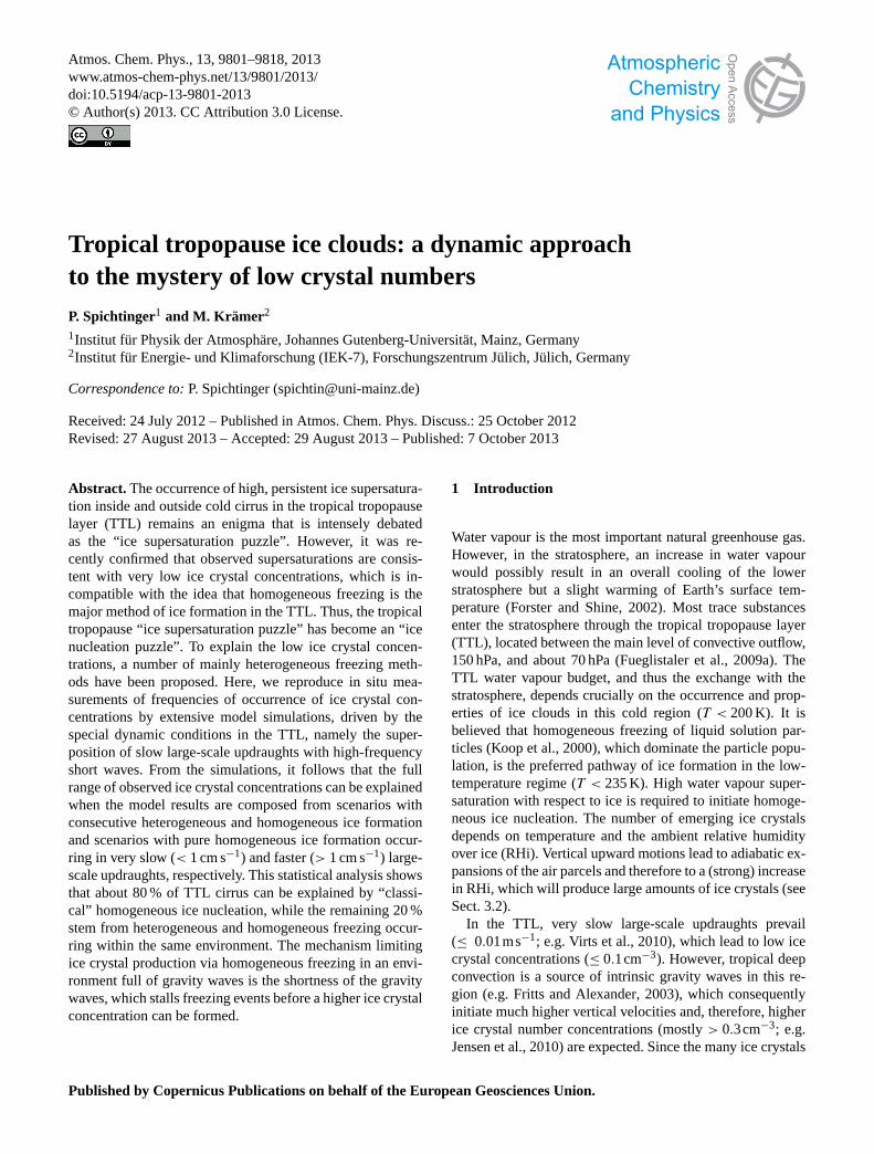
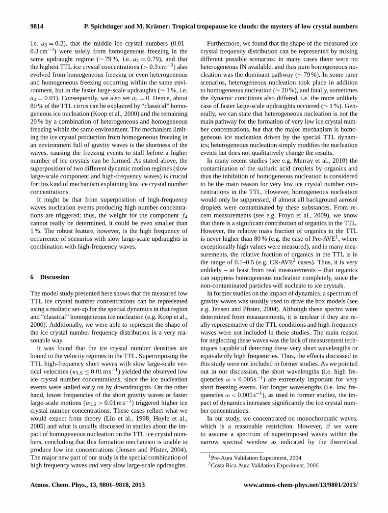
For this purpose, we simulated a situation of a constantupdraught, i.e. a standard cooling event, indicated by redlines in all three panels of Fig.1. The box model is usedincluding processes of (a) homogeneous freezing of aque-ous solution droplets and (b) diffusional growth/evaporationonly; sedimentation is ignored in order to reduce the com-plexity of the experiment. We specified one class of homo-geneously frozen ice crystals. For the soluble backgroundaerosol, which forms the solution droplets that trigger ho-mogeneous nucleation later on, we prescribed a dry H2SO4aerosol with lognormal distribution, a geometric standard de-viation ofσr = 1.5, and initial modal radiusrm = 25nm. Thebackground aerosol number concentration was set toNa =
300cm−3, which is more representative for extra-tropical tro-pospheric conditions. For the standard cooling event withinitial conditions ofTinit = 220 K andpinit = 300 hPa, anda prescribed persistent updraught ofw = 0.1ms−1, the rel-ative humidity increased (red line in upper panel of Fig.1).At some point, the threshold RHi for homogeneous nucle-ation of droplets of a certain size (black line: threshold for∼ 250 nm droplets) was reached and thus ice crystals wereformed via homogeneous freezing. However, these ice crys-tals were quite small. Their surface was small so that theirability to deplete water vapour was quite limited; therefore,the relative humidity continued to increase; i.e. the sourceof supersaturation due to adiabatic cooling dominated overthe sink of diffusional growth. The increasing relative hu-midity led to further ice crystal nucleation. After some time(aroundt ∼ 350 s), the size of the ice crystals increased, al-lowing the crystals to deplete the water vapour efficiently,balancing the source via adiabatic cooling. Aftert ∼ 355 s,the sink was stronger than the source and the relative hu-midity decreased (i.e. there was a net sink), although therewas still a source of supersaturation by adiabatic cooling. At
www.atmos-chem-phys.net/13/9801/2013/ Atmos. Chem. Phys., 13, 9801–9818, 2013
9804 P. Spichtinger and M. Krämer: Tropical tropopause ice clouds: the mystery of low crystal numbers
150
150.5
151
151.5
152
152.5
153
153.5
154
180 240 300 360 420 480
rela
tive
hum
idity
ove
r ic
e (%
)
time (s)
(a) persistentchanging
RHihom
0.001
0.01
0.1
1
10
180 240 300 360 420 480
ice
crys
tal n
ucle
atio
n ra
te (
L-1s-1
)
time (s)
(b)
� 140 sec
persistentchanging
dN/dt equiv to RHihomτnuc
0
20
40
60
80
100
120
180 240 300 360 420 480
ice
crys
tal n
umbe
r co
ncen
trat
ion
(L-1
)
time (s)
(c) persistentchanging
Fig. 1. Example of the impact of changing updraughts on the formation of ice crystals via homogeneous freezing of solution droplets. Thethree panels show the time evolution of(a) relative humidity with respect to ice,(b) ice crystal nucleation rate, and(c) ice crystal numberconcentration. Red curves indicate a constant persistent updraught ofw = 0.1ms−1, whereas blue curves indicate a scenario with a constantupdraught ofw = 0.1ms−1 until t = 320 s, followed by a constant downdraught ofw = −0.1ms−1. The black line in panel(a) indicatesthe homogeneous nucleation threshold for solution droplets of sizer = 0.25 µm; this threshold corresponds to a production rate of dNi/dt =
0.04L−1s−1 as indicated in panel(b).
later times, the relative humidity crossed the homogeneousnucleation threshold, approaching from higher values, thusice crystal formation was shut down. Until this threshold wasreached, there was still ice crystal nucleation. This scenario isused quite often in many idealized studies in order to investi-gate ice formation at constant updraughts under certain con-ditions (see, e.g.Kärcher and Lohmann, 2002; Hoyle et al.,2005; Barahona and Nenes, 2008; Spichtinger and Gierens,2009a; Spichtinger and Cziczo, 2010), leading to a one-to-one relationship between vertical updraughts and ice crys-tal number concentrations produced in such cooling events.The main issue here is that the vertical updraught was keptconstant during the whole cooling event, which lasted aboutτnuc ≈ 140 s. In the middle panel of Fig.1, the ice crystalnucleation rate is shown, including the nucleation timeτnuc,whereas in the right panel of the figure, the evolution of theice crystal number concentration is shown. Since we show ascenario at quite high temperatures (initiallyT = 220 K), theice crystal number concentration formed in the cooling eventis quite low (N ≈ 105L−1).
Next, we will look at the case of a change in vertical up-draught during the nucleation event (i.e. within the time in-terval τnuc). To demonstrate this issue, we investigated thefollowing idealized scenario. We started with a constant up-draught ofw = 0.1ms−1, but att = 320 s we switched to thevalue ofw = −0.1ms−1, i.e. the updraught was turned into adowndraught of equal strength (Fig.1, blue lines). Until thechange in updraught, the simulations were identical. How-ever, when the cooling process was turned into a warmingprocess, the relative humidity decreased at approximately thesame rate as it increased before. The homogeneous nucle-ation threshold was reached soon after this (att ∼ 355 s, in-cidentally approximately the time where the maximum RHivalues were reached in the reference simulation), thus the
nucleation event was stopped much earlier, as can be seenin the ice crystal nucleation rate in the middle panel. Thisled to a significantly lower ice crystal number concentration,compared to the reference simulation. When vertical veloc-ities were modified fromw = 0.1ms−1 to w = −0.1ms−1
during the nucleation event, the final ice crystal number con-centration was aboutN ≈ 20L−1.
The key finding of these investigations is that a changingvertical updraught could massively influence the number ofice crystals produced during a nucleation event. This findingwas used to simulate the small ice crystal number concentra-tions found in the TTL. The updraught was then modified bysuperimposing a wave structure to a very slow vertical mo-tion. As we will show later (Sect.4), a varying updraught inthe TTL is triggered by high-frequency gravity waves.
3 Idealized TTL ice cloud simulations
In this section, the role of different superimposed vertical ve-locity components in the formation of ice crystals will be in-vestigated by means of idealized model simulations relevantto the situation in the TTL.
3.1 Model set-up
To perform the idealized TTL ice cloud simulations, we usedthe box model described in Sect.2.1 with the followingmodel set-up: as in the simulations described in the previ-ous section, only one class of ice formed by homogeneousnucleation was assumed; the same background aerosol con-ditions were prescribed as in Sect.2; i.e. we assume pure ho-mogeneous freezing of aqueous solution droplets containingsulfuric acid. In a first step, we established a reliable rela-tionship between vertical updraught and ice crystal number
Atmos. Chem. Phys., 13, 9801–9818, 2013 www.atmos-chem-phys.net/13/9801/2013/
P. Spichtinger and M. Krämer: Tropical tropopause ice clouds: the mystery of low crystal numbers 9805
concentrations for the temperature range 185≤ T ≤ 200 Kand the vertical velocity range of 0.01≤ w ≤ 10ms−1. Inour model simulations, the aerosol particles were removedfrom the background as soon as ice crystals were formed.Hence, the background aerosol was reduced during nucle-ation events and acted as a limiting factor for the ice crys-tal number concentrations formed. As the initial pressure ofall simulations we usedpinit = 100 hPa, motivated by aircraftmeasurements (see, e.g.Schiller et al., 2008).
In a second step, we investigated the influence of chang-ing updraughts in a more relevant but still idealized set-up.For this purpose, we specified two different types of verticalvelocity; a large-scale componentwLS and a wave-like sig-nature, given by a pure sine wave. According to Eq. (6) thechange in relative humidity is driven by temperature changes,which correspond to vertical velocity via Eq. (5) assumingadiabatic changes. The temperature evolution for the spe-cial case of a large-scale updraught superimposed by a high-frequency monochromatic wave with an intrinsic frequencyω =
2πτ
can be described as follows:
T (t) = Tinit −0 · wLS · t︸ ︷︷ ︸large scale
+AT cos(ωt)︸ ︷︷ ︸wave
(7)
= Tinit + TLS(t) + Twave(t). (8)
Thus, the temperature rate is given by the following equation:
dT
dt= −0 · wLS︸ ︷︷ ︸
large scale
−ATωsin(ωt)︸ ︷︷ ︸wave
=dT
dt
∣∣∣large scale
+dT
dt
∣∣∣wave.
(9)
Using Eq. (5) we end up with an expression for the verticalvelocity, which is consistent with Eq. (7):
w(t) =dz
dt= wLS +
cp
gωAT sin(ωt) (10)
= wLS + Aw sin(ωt) = wLS + wwave(t). (11)
For our idealized set-up we choose a time period ofτ =
500 s, i.e.ω =2πτ
≈ 0.0126s−1; the amplitude is set to avalue of Aw = 1.25ms−1, corresponding to a temperatureamplitude of aboutAT ≈ 1 K. For the large-scale compo-nent we distinguished between two different regimes, i.e. alow regime (wLS = 0.008ms−1) and a high regime (wLS =
0.03ms−1). In Sect.5, we will show that the choice of thesevalues was not arbitrary but motivated by the realistic dy-namic conditions in the TTL (see Sect.4).
3.2 Results
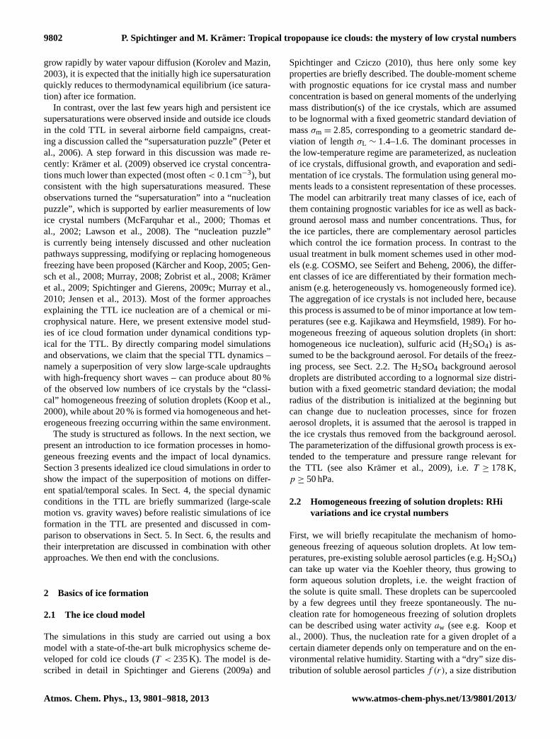
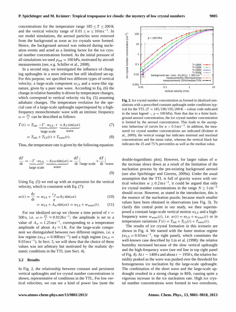
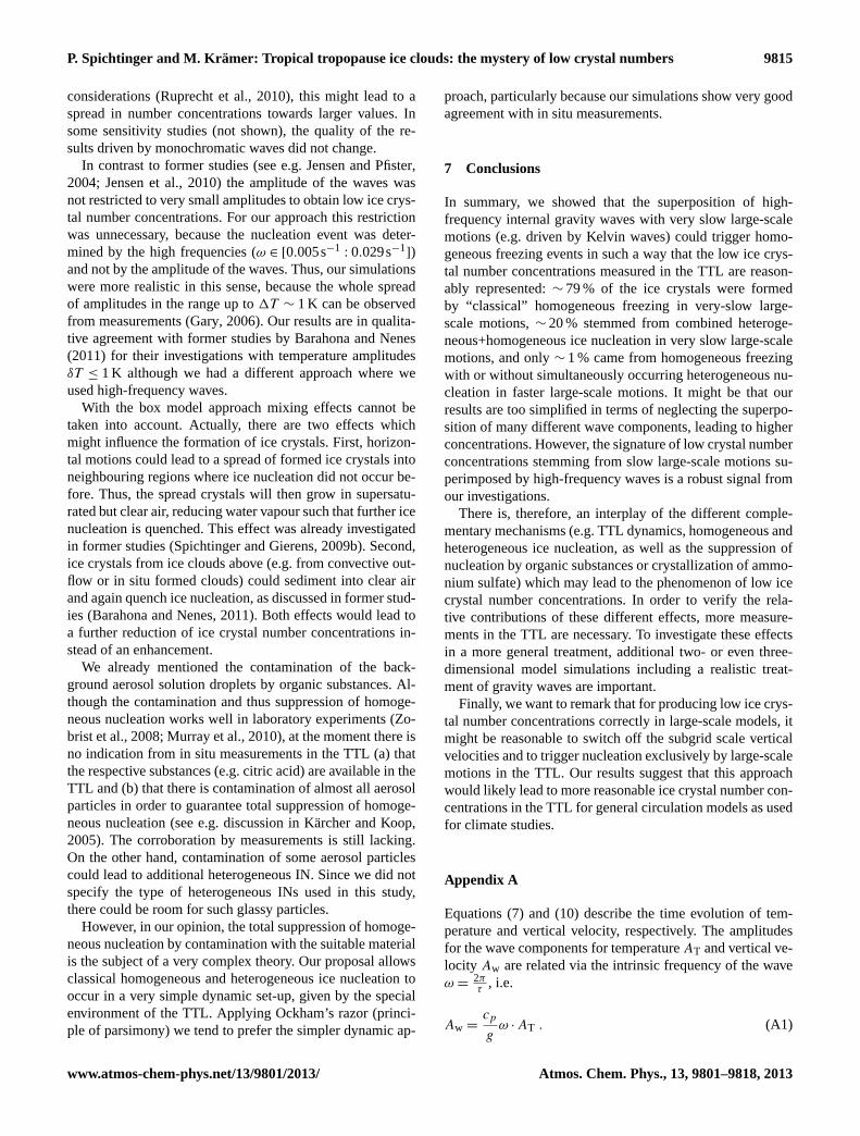
In Fig. 2, the relationship between constant and persistentvertical updraughts and ice crystal number concentrations isshown, representative of conditions in the TTL. For low ver-tical velocities, we can see a kind of power law (note the
0.001
0.01
0.1
1
10
100
0.01 0.1 1 10
ice
crys
tal n
umbe
r co
ncen
trat
ion
(cm
-3)
vertical velocity (m/s)
p = 100 hPa
T=185KT=190KT=195KT=200K
background aer. conc. (H2SO4) = 300 cm-3
measurements min/mean/maxmeasurements 25%/median/75%
Fig. 2. Ice crystal number concentration as formed in idealized sim-ulations with a prescribed constant updraught under conditions typ-ical for the TTL (T = 185/190/195/200 K – colour code indicatedin the inset legend –,p = 100 hPa). Note that due to a finite back-ground aerosol concentration, the ice crystal number concentrationis limited by the aerosol concentration. This leads to the asymp-totic behaviour of curves forw > 0.5ms−1. In addition, the mea-sured ice crystal number concentrations are indicated (Krämer etal., 2009); the vertical orange bar indicates minimal and maximalconcentrations and the mean value, whereas the vertical black barindicates the 25 and 75 % percentiles as well as the median value.
double-logarithmic plot). However, for larger values ofw
the increase slows down as a result of the limitation of thenucleation process by the pre-existing background aerosol(see alsoSpichtinger and Gierens, 2009a). Under the usualassumption that the TTL is full of gravity waves with ver-tical velocitiesw ≥ 0.2ms−1, it could be argued that onlyice crystal number concentrations in the rangeN ≥ 1cm−3
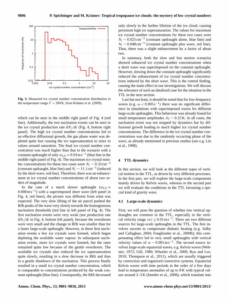
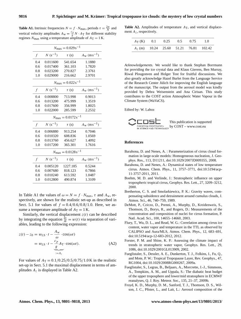
should occur. However, as stated in the introduction, this isthe essence of the nucleation puzzle, because much smallervalues have been obtained in observations (see Fig.3). Toclarify this central point in our study, we then superim-posed a constant large-scale vertical motionwLS and a high-frequency wavewwave(t), i.e. w(t) = wLS + wwave(t) or intemperature variationsT (t) = Tinit + TLS(t) + Twave(t).
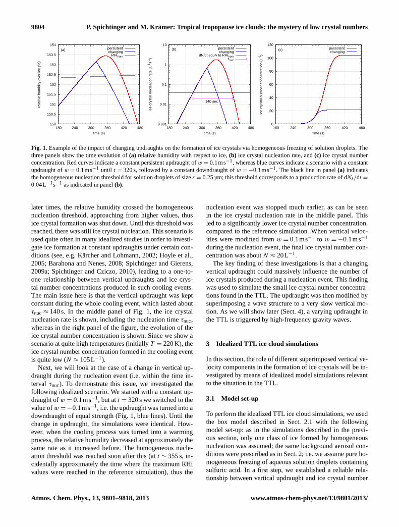
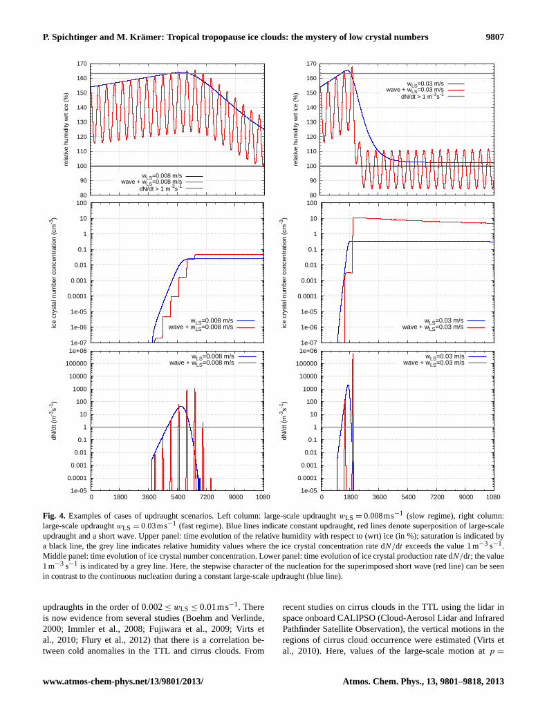
The results of ice crystal formation in this scenario areshown in Fig.4. We started with the faster motion regime(wLS = 0.03ms−1, top right panel), which constitutes thewell-known case described byLin et al. (1998): the relativehumidity increased because of the slow vertical updraughtand the high-frequency wave (see red line in top right panelof Fig.4). At t ∼ 1400 s and aboutt ∼ 1950 s, the relative hu-midity peaked as the wave was pushed over the threshold forhomogeneous ice nucleation by the large-scale updraught.The combination of the short wave and the large-scale up-draught resulted in a strong change in RHi, causing quite avigorous increase in the ice nucleation rate. High ice crys-tal number concentrations were formed in two overshoots,
www.atmos-chem-phys.net/13/9801/2013/ Atmos. Chem. Phys., 13, 9801–9818, 2013
9806 P. Spichtinger and M. Krämer: Tropical tropopause ice clouds: the mystery of low crystal numbers
0.01
0.1
1
10
100
0.001 0.01 0.1 1 10 100
freq
uenc
y of
occ
urre
nce
(%)
ice crystal number concentration (cm-3)
measurements
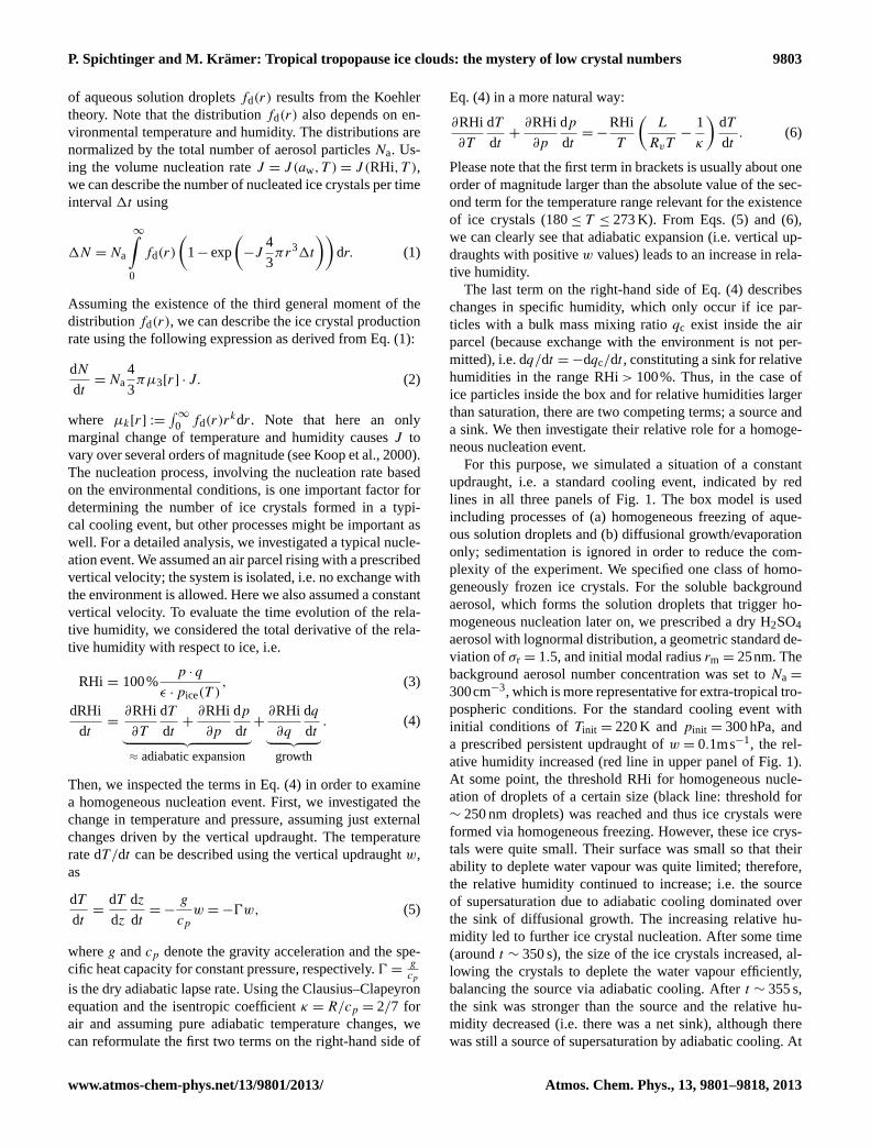
Fig. 3. Measured ice crystal number concentration distribution inthe temperature rangeT < 200 K, fromKrämer et al.(2009).
which can be seen in the middle right panel of Fig.4 (redline). Additionally, the two nucleation events can be seen inthe ice crystal production rate dNi/dt (Fig. 4, bottom rightpanel). The high ice crystal number concentrations led toan effective diffusional growth, the gas phase water was de-pleted quite fast causing the ice supersaturation to relax tovalues around saturation. The final ice crystal number con-centration was much higher than that in the scenario with aconstant updraught of onlywLS = 0.03ms−1 (blue line in themiddle right panel of Fig.4). The maximum ice crystal num-ber concentrations for these two cases wereNi ∼ 0.33cm−3
(constant updraught, blue line) andNi ∼ 11.1cm−3 (inducedby the short wave, red line). Therefore, there was an enhance-ment in ice crystal number concentrations of about two or-ders of magnitude.
In the case of a much slower updraught (wLS =
0.008ms−1) with a superimposed short wave (left panel inFig. 4, red lines), the picture was different from what wasexpected. The very slow lifting of the air parcel pushed theRHi peaks of the wave very slowly towards the homogeneousnucleation thresholds (red line in left panel of Fig.4). Thefirst nucleation events were very weak (see production ratedNi/dt in Fig. 4, bottom left panel), because the overshootswere very small and the change in RHi was smaller than fora faster large-scale updraught. However, in these first nucle-ation events a few ice crystals were formed, which begandepleting the available water vapour. In subsequent nucle-ation events, more ice crystals were formed, but the ratesremained quite low because of the gentle overshoots. Theavailable ice crystals also reduced the ice supersaturationquite slowly, resulting in a slow decrease in RHi and thusin a gentle shutdown of the nucleation. This process finallyresulted in a small ice crystal number concentration, whichis comparable to concentrations produced by the weak con-stant updraught (blue line). Consequently, the RHi decreased
only slowly in the further lifetime of the ice cloud, causingpersistent high ice supersaturation. The values for maximumice crystal number concentrations for these two cases wereNi ∼ 0.025cm−3 (constant updraught alone, blue line) andNi ∼ 0.048cm−3 (constant updraught plus wave, red line).Thus, there was a slight enhancement by a factor of abouttwo.
In summary, both the slow and fast motion scenariosshowed enhanced ice crystal number concentrations whena short wave was superimposed on the constant updraught.However, slowing down the constant updraught significantlyreduced the enhancement of ice crystal number concentra-tions induced by the short wave. This is the central finding,causing the main effect in our investigations. We will discussthe relevance of such an idealized case for the situation in theTTL in the next section.
Last but not least, it should be noted that for low-frequencywaves (e.g.ω < 0.005s−1) there was no significant differ-ence in simulations with superimposed waves for differentlarge-scale updraughts. This behaviour was already found forsmall temperature amplitudesAT ∼ 0.25 K. In all cases, thenucleation event was not stopped by dynamics but by dif-fusional growth leading to much higher ice crystal numberconcentrations. The difference in the ice crystal number con-centrations was due to the randomly occurring phase of thewave, as already mentioned in previous studies (see e.g.Linet al., 1998).
4 TTL dynamics
In this section, we will look at the different types of verti-cal motion in the TTL, as driven by very different processes.In the first part, we will explore the large-scale componentsmainly driven by Kelvin waves, whereas in the second partwe will evaluate the conditions in the TTL favouring a spe-cial kind of gravity wave.
4.1 Large-scale dynamics
First, we will pose the question of whether low vertical up-draughts are common in the TTL, especially in the verti-cal velocity range|w| ≤ 0.01ms−1. There are two differentsources for large-scale updraughts in the TTL. The first in-volves ascents to compensate diabatic heating (e.g.Salbyand Callaghan, 2004; Fueglistaler et al., 2009b); this com-pensating effect led to very small updraughts with verticalvelocity values ofw ∼ 0.001ms−1. The second source in-volves large-scale equatorial waves, e.g. Kelvin waves (Web-ster, 1972; Gill , 1980; Wheeler et al., 2000; Ryu and Lee,2010; Thompson et al., 2011), which are usually triggeredby convection and organized convective systems. EquatorialKelvin waves with time periods in the order of a few dayslead to temperature anomalies of up to 8 K with typical val-ues around 2–3 K (Immler et al., 2008), which translate into
Atmos. Chem. Phys., 13, 9801–9818, 2013 www.atmos-chem-phys.net/13/9801/2013/
P. Spichtinger and M. Krämer: Tropical tropopause ice clouds: the mystery of low crystal numbers 9807
80
90
100
110
120
130
140
150
160
170
0 1800 3600 5400 7200 9000 10800
rela
tive
hum
idity
wrt
ice
(%)
time (s)
wLS=0.008 m/swave + wLS=0.008 m/s
dN/dt > 1 m-3s-1
80
90
100
110
120
130
140
150
160
170
0 1800 3600 5400 7200 9000 10800
rela
tive
hum
idity
wrt
ice
(%)
time (s)
wLS=0.03 m/swave + wLS=0.03 m/s
dN/dt > 1 m-3s-1
1e-07
1e-06
1e-05
0.0001
0.001
0.01
0.1
1
10
100
0 1800 3600 5400 7200 9000 10800
ice
crys
tal n
umbe
r co
ncen
trat
ion
(cm
-3)
time (s)
wLS=0.008 m/swave + wLS=0.008 m/s
1e-07
1e-06
1e-05
0.0001
0.001
0.01
0.1
1
10
100
0 1800 3600 5400 7200 9000 10800
ice
crys
tal n
umbe
r co
ncen
trat
ion
(cm
-3)
time (s)
wLS=0.03 m/swave + wLS=0.03 m/s
1e-05
0.0001
0.001
0.01
0.1
1
10
100
1000
10000
100000
1e+06
0 1800 3600 5400 7200 9000 10800
dN/d
t (m
-3s-1
)
time (s)
wLS=0.008 m/swave + wLS=0.008 m/s
1e-05
0.0001
0.001
0.01
0.1
1
10
100
1000
10000
100000
1e+06
0 1800 3600 5400 7200 9000 10800
dN/d
t (m
-3s-1
)
time (s)
wLS=0.03 m/swave + wLS=0.03 m/s
Fig. 4. Examples of cases of updraught scenarios. Left column: large-scale updraughtwLS = 0.008ms−1 (slow regime), right column:large-scale updraughtwLS = 0.03ms−1 (fast regime). Blue lines indicate constant updraught, red lines denote superposition of large-scaleupdraught and a short wave. Upper panel: time evolution of the relative humidity with respect to (wrt) ice (in %); saturation is indicated bya black line, the grey line indicates relative humidity values where the ice crystal concentration rate dN/dt exceeds the value 1 m−3 s−1.Middle panel: time evolution of ice crystal number concentration. Lower panel: time evolution of ice crystal production rate dN/dt ; the value1 m−3 s−1 is indicated by a grey line. Here, the stepwise character of the nucleation for the superimposed short wave (red line) can be seenin contrast to the continuous nucleation during a constant large-scale updraught (blue line).
updraughts in the order of 0.002≤ wLS ≤ 0.01ms−1. Thereis now evidence from several studies (Boehm and Verlinde,2000; Immler et al., 2008; Fujiwara et al., 2009; Virts etal., 2010; Flury et al., 2012) that there is a correlation be-tween cold anomalies in the TTL and cirrus clouds. From
recent studies on cirrus clouds in the TTL using the lidar inspace onboard CALIPSO (Cloud-Aerosol Lidar and InfraredPathfinder Satellite Observation), the vertical motions in theregions of cirrus cloud occurrence were estimated (Virts etal., 2010). Here, values of the large-scale motion atp =
www.atmos-chem-phys.net/13/9801/2013/ Atmos. Chem. Phys., 13, 9801–9818, 2013
9808 P. Spichtinger and M. Krämer: Tropical tropopause ice clouds: the mystery of low crystal numbers
100 hPa were estimated to be in the range−0.0175Pas−1≤
ω ≤ 0 (see fig. 8.8 inVirts, 2009), which translates into ver-tical velocities in the range 0≤ w ≤ 0.01ms−1. Thus, fromobservational and theoretical considerations, the occurrenceof low large-scale motions in the range 0≤ w ≤ 0.01ms−1
can be confirmed and the occurrence of cirrus clouds insuch updraught regions is quite common. It should be men-tioned here that in case of large-scale updraughts in the range0 ≤ w ≤ 0.01ms−1 without any superposition of motions onsmaller scales, only small ice crystal number concentrations(Ni ≤ 0.1cm−3) would occur, as can be derived in Fig.2.Additionally, it seems that large-scale motions with verticalvelocities ofw > 0.01 m s−1 are quite rare. This will be im-portant in the following discussion.
In our simulations (see Sect.5) we will always assume thatvertical motions are consistent with adiabatic changes lead-ing to temperature variations. Strictly speaking, this is onlytrue for the second component (Kelvin waves), whereas thediabatic heating compensating would be associated with alapse ratedT
dz> −0, leading to smaller cooling rates. Since
the vertical velocity driven by diabatic heating effects isusually much smaller than the component driven by Kelvinwaves, we can neglect this contribution and assume adiabaticchanges to a very good approximation.
4.2 Gravity waves
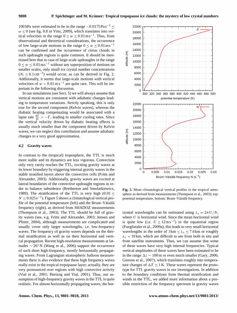
In contrast to the (tropical) troposphere, the TTL is muchmore stable and its dynamics are less vigorous. Convectiononly very rarely reaches the TTL, exciting gravity waves atits lower boundary by triggering internal gravity waves in thestable stratified layers above the convective cells (Fritts andAlexander, 2003). Additionally, gravity waves are excited atlateral boundaries of the convective updraught regions in or-der to balance subsidence (Bretherton and Smolarkiewicz,1989). The stratification of the TTL is very high (0.01≤
N ≤ 0.025s−1). Figure5shows a climatological vertical pro-file of the potential temperature (left) and the Brunt–Väisäläfrequency (right), as derived from SHADOZ measurements(Thompson et al., 2003). The TTL should be full of grav-ity waves (see, e.g.Fritts and Alexander, 2003; Jensen andPfister, 2004), although measurements are complicated andusually cover only larger wavelengths, i.e. low-frequencywaves. The frequency of gravity waves depends on the ther-mal stratification as well as on their horizontal and verti-cal propagation. Recent high-resolution measurements at lat-itudes∼ 26◦ N (Wang et al., 2006) support the occurrenceof such short high-frequency, mostly horizontally propagat-ing waves. From Lagrangian stratospheric balloon measure-ments there is also evidence that these high frequency wavesreally exist in the tropical tropopause layer; actually, they arevery pronounced over regions with high convective activity(Vial et al., 2001; Hertzog and Vial, 2001). Thus, our as-sumption of high-frequency gravity waves in the TTL is quiterealistic. For almost horizontally propagating waves, the hor-
0
2000
4000
6000
8000
10000
12000
14000
16000
18000
20000
22000
300 320 340 360 380 400 420 440 460 480 500
altit
ude
(m)
potential temperature (K)
θ
0
2000
4000
6000
8000
10000
12000
14000
16000
18000
20000
22000
0 0.005 0.01 0.015 0.02 0.025 0.03
altit
ude
(m)
Brunt−Väisälä frequency N (s−1)
N
Fig. 5. Mean climatological vertical profiles in the tropical atmo-sphere as derived from measurements (Thompson et al., 2003); top:potential temperature, bottom: Brunt–Väisälä frequency.
izontal wavelengths can be estimated usingλx = 2πU/N ,whereU is horizontal wind. Since the mean horizontal windis quite low (i.e. U ≤ 12ms−1) in the equatorial region(Fueglistaler et al., 2009a), this leads to very small horizontalwavelengths in the order of 3km≤ λx ≤ 7.6km or roughlyλx < 10 km, which are difficult to see from both in situ andfrom satellite instruments. Thus, we can assume that someof these waves have very high internal frequencies. Typicalvertical amplitudes of these waves have been estimated to bein the range1z ∼ 100 m or even much smaller (Gary, 2006;Gierens et al., 2007), which translates roughly into tempera-ture changes of1T ≤ 1 K. These waves represent the proto-type for TTL gravity waves in our investigations. In additionto the boundary conditions from thermal stratification andwinds in the TTL, we added more information about a pos-sible restriction of the frequency spectrum in gravity waves
Atmos. Chem. Phys., 13, 9801–9818, 2013 www.atmos-chem-phys.net/13/9801/2013/
P. Spichtinger and M. Krämer: Tropical tropopause ice clouds: the mystery of low crystal numbers 9809
occurring. From recent theoretical investigations (Ruprechtet al., 2010; Ruprecht and Klein, 2011) on the propagationin the gravity waves in a convectively dominated environ-ment, we know that the full spectrum of frequencies, i.e.0 ≤ ω ≤ N , does not occur. The convective towers act ashigh-pass filters, depending on the fractional coverage of theconvective cells compared to the cloud-free environment, al-lowing only part of the frequency to occur. The frequencyspectrum is then given byf · N ≤ ω ≤ N , wheref dependson the fractional coverageσ , i.e.f ≈
√σ . For typical values
of σ ∼ 0.1, we get a frequency cut-off factor off ≈ 0.32.Since there is a lot of convective activity in the tropical re-gions, we can assume higher fractional coverage of convec-tive cells. Thus,σ = 0.1 is a lower limit. In later applica-tions of this “frequency window”, we will use a lower limitof f = 0.4, i.e. f will be in the range 0.4 ≤ f ≤ 1, corre-sponding to cloud cover values of∼ 0.16≤ σ ≤ 1. Unfor-tunately, there are no direct in situ observations of verticalvelocity, thus we cannot compare our dynamical set-up andresults with measurements.
5 Realistic TTL ice cloud simulations
After observations and theoretical investigations have shownthat the conditions as specified in Sect.3 may occur in theTTL, we will now define more realistic scenarios for a largenumber of box model simulations. The results of these simu-lations will be presented in terms of ice crystal number con-centrations. Additionally, we will discuss the plausibility ofheterogeneous ice nucleation for the situation in the TTL.
5.1 Model set-up
For the realistic model simulations, we ran the ice cloud boxmodel along idealized air mass trajectories. The set-up forthe microphysics as well as for the idealized dynamics, i.e.trajectories, is described in the next two subsections.
5.1.1 Model set-up for microphysics
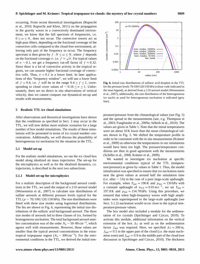
For a realistic description of the background aerosol condi-tions in the TTL, we used the output of a 2-D aerosol model(Weisenstein et al., 2007) to calculate size distributions ofsulfate aerosols at different pressure levels typical for theTTL (p ∼ 70/100/120/150 hPa). The size distributions werefitted with three size modes using lognormal distributions.The fits are shown in Fig.6, representing the initial size dis-tributions of the sulfuric acid background aerosol. The threesize modes of aerosols led to three classes of ice, formed byhomogeneous nucleation. The total background aerosol num-ber concentration was of the orderNa ∼ 50–80 cm−3, whichagrees well with measurements. However, these values aresmaller than the typical aerosol concentrations in the extra-tropical tropopause region (Na ∼ 300cm−3). For the envi-ronmental conditions in the TTL, we derived the initial tem-
0.0001
0.001
0.01
0.1
1
10
100
1 10 100 1000
num
ber
conc
entr
atio
n (c
m-3
)
radius (nm)
p=70-150hPa
hom. modes, 150hPahom. modes, 120hPahom. modes, 100hPahom. modes, 70 hPa
het. mode
Fig. 6. Initial size distributions of sulfuric acid droplets in the TTLfor the pressure levels 70/100/120/150 hPa (colour code indicated inthe inset legend), as derived from a 2-D aerosol model (Weisensteinet al., 2007); additionally, the size distribution of the heterogeneousice nuclei as used for heterogeneous nucleation is indicated (greyline).
perature/pressure from the climatological values (see Fig.5)and the spread in the measurements (see, e.g.Thompson etal., 2003; Fueglistaler et al., 2009a; Selkirk et al., 2010). Thevalues are given in Table1. Note that the initial temperatureswere set about 10 K lower than the mean climatological val-ues shown in Fig.5. We shifted the temperature profile inorder to be consistent with the in situ measurements (Krämeret al., 2009) as otherwise the temperatures in our simulationswould have been too high. The pressure/temperature con-ditions are then in good agreement with the measurements(Schiller et al., 2008; Krämer et al., 2009).
We wanted to investigate ice nucleation at specificenvironmental conditions typical of the TTL (tempera-ture/pressure) as given by values in Table1. Thus, the modelinitialization was specified to ensure that ice nucleation startsnear the given values at around half the simulation time(i.e. after∼ 5 h) in the case of a pure large-scale updraught.For example, whenTnuc = 196 K andpnuc = 150 hPa witha constant updraught ofwLS = 0.01ms−1, we setTinit =
197.8 K and pinit = 154.78 hPa. Using this procedure, weensured that when high-frequency waves with high ampli-tudes were superimposed to the large-scale updraught (seeSect.5.1.2) nucleation would occur close to the typical tem-perature/pressure values.
The box model also included a module for the sedimen-tation of ice crystals (Spichtinger and Cziczo, 2010). Toactivate this module, additional information on the verticalextension of the box1z as well as on the sedimentationfactor fsed was required. Here, we specified1z = 200 m,fsed= 0.5 in the upper part of the cloud (i.e. the main nucle-ation zone) andfsed= 0.9 in the middle part of the cloud (seediscussion inSpichtinger and Cziczo, 2010). The thickness
www.atmos-chem-phys.net/13/9801/2013/ Atmos. Chem. Phys., 13, 9801–9818, 2013
9810 P. Spichtinger and M. Krämer: Tropical tropopause ice clouds: the mystery of low crystal numbers
Table 1. Settings for realistic simulations to be fulfilled at ice nu-cleation.
p (hPa) 70 100 120 150
T (K) 190 184 188 196
Nmax (s−1) 0.029 0.022 0.0172 0.0128Nmean= Nmax· 0.9 (s−1) 0.0261 0.0198 0.0155 0.0115Nmin = Nmax· 0.4 (s−1) 0.0116 0.0088 0.0069 0.0051
of the cloud layers are based on recent measurements byJensen et al.(2013), indicating layers with a vertical exten-sion in the order ofO(100–500 m).
5.1.2 Model set-up for dynamics
We saw in Sect.4 that the TTL dynamics were dominated bymotions on two different scales, namely (a) very low large-scale updraughts in the order ofwLS ≤ 1cms−1 and (b) high-frequency gravity waves triggered by convective activity. Thelarge-scale updraughts were triggered by large-scale featuressuch as Kelvin waves, occupying large horizontal regions inthe tropical atmosphere. Thus, gravity waves are embeddedinto the slowly lifted environment. In terms of an ascend-ing air parcel along a trajectory, we thus assumed a slowlylifted parcel, which also experiences a superimposed (high-frequency) oscillation driven by gravity waves. As describedabove, the source for the gravity waves is most likely convec-tion. Either waves are triggered by convective plumes bounc-ing against the TTL from below or waves are radiated lat-erally from the convective tower. In both cases, we can as-sume intrinsic gravity waves with frequencies near the ther-mal stratification of the TTL (i.e.ω ≈ N ). Thus, in our sim-ulations we concentrated on monochromatic waves with adistinct frequency as determined below. For our box modelcalculations we specified – similar to the idealized simula-tions in Sect.3 – a vertical velocity for lifting the (closed)air parcel adiabatically as a superposition of the two motionsmentioned above:w(t) = wLS + wwave(t), i.e. expressed asvertical velocities, which are more natural in a dynamicalpoint of view. For the large-scale componentwLS we thenspecified the following ranges, split into a very slow and afaster velocity range:
wLS = 0.003/0.005/0.008/0.01︸ ︷︷ ︸very slow
/0.02/0.03/0.05︸ ︷︷ ︸faster
ms−1 .
(12)
Hence, to determine the monochromatic wave componentwwave(t), we use again temperature changes (T (t) = Tinit +
TLS(t) + Twave(t)) instead of changes in the vertical veloc-ity; this approach is also due to observational constraints onthe amplitude of temperature variations in the TTL. We as-sumed an adiabatic process; i.e. that the vertical velocity was
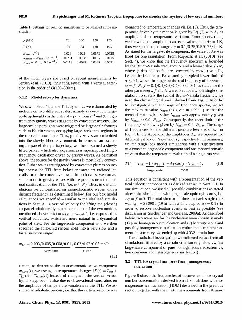
connected to temperature changes via Eq. (5). Thus, the tem-perature driven by this motion is given by Eq. (7) with AT asamplitude of the temperature variation. From observations,we know that the amplitude can reach values up toAT = 1 K,thus we specified the rangeAT = 0.1/0.25/0.5/0.75/1.0 K.As stated for the large-scale component, the value ofAT wasfixed for one simulation. FromRuprecht et al.(2010) (seeSect.4), we know that the frequency spectrum is boundedby the Brunt–Väisälä frequencyN and a lower valuef · N ,wheref depends on the area covered by convective cells,i.e. on the fractionσ . By assuming a typical lower limit ofσ ≤ 0.1, we set the range for the real frequency of the waves,ω = f ·N , f = 0.4/0.5/0.6/0.7/0.8/0.9/1; as stated for theother parameters,f andN were fixed for a whole single sim-ulation. To specify the typical Brunt–Väisälä frequency, weused the climatological mean derived from Fig.5. In orderto investigate a realistic range of frequency spectra, we setthe maximum valueNmax (as given in Table1) so that themean climatological valueNmean was approximately givenby Nmean≈ 0.9 · Nmax. Consequently, the lower limit of thefrequency window is given byNmin = 0.4 · Nmax. The rangeof frequencies for the different pressure levels is shown inFig. 7. In the Appendix, the amplitudesAw are reported fordifferent values ofNmax and f , respectively. In summary,we ran single box model simulations with a superpositionof a constant large-scale component and one monochromaticwave so that the temperature evolution of a single run was
T (t) = Tinit −0 · wLS · t︸ ︷︷ ︸large scale
+AT cos(f · Nmax · t)︸ ︷︷ ︸wave
. (13)
This equation is consistent with a representation of the ver-tical velocity components as derived earlier in Sect.3.1. Inour simulations, we used all possible combinations as statedabove plus simulations with large-scale updraughts only, i.e.AT = f = 0. The total simulation time for each single casewas tsim = 36000 s (10 h) with a time step of1t = 0.1 s inorder to resolve nucleation events as best as possible (seediscussion inSpichtinger and Gierens, 2009a). As describedbelow, two scenarios for the nucleation were chosen, namely(1) pure homogeneous nucleation and (2) heterogeneous andpossibly homogeneous nucleation within the same environ-ment. In summary, we ended up with 4 032 simulations.
For a statistical investigation, we collected values from allsimulations, filtered by a certain criterion (e.g. slow vs. fastlarge-scale component or pure homogeneous nucleation vs.homogeneous and heterogeneous nucleation).
5.2 TTL ice crystal numbers from homogeneousnucleation
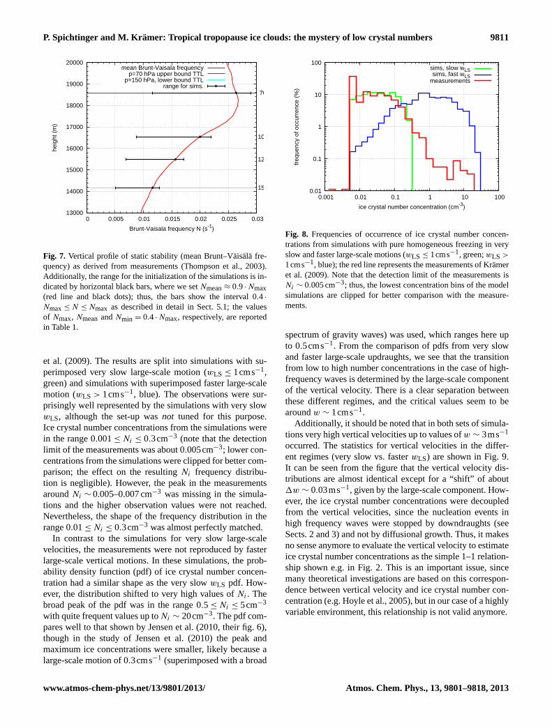
Figure8 shows the frequencies of occurrence of ice crystalnumber concentrations derived from all simulations with ho-mogeneous ice nucleation (HOM) described in the previoussection together with the in situ measurements fromKrämer
Atmos. Chem. Phys., 13, 9801–9818, 2013 www.atmos-chem-phys.net/13/9801/2013/
P. Spichtinger and M. Krämer: Tropical tropopause ice clouds: the mystery of low crystal numbers 9811
13000
14000
15000
16000
17000
18000
19000
20000
0 0.005 0.01 0.015 0.02 0.025 0.03
heig
ht (
m)
Brunt-Vaisala frequency N (s-1)
70 hPa
100 hPa
120 hPa
150 hPa
mean Brunt-Vaisala frequencyp=70 hPa upper bound TTL
p=150 hPa, lower bound TTLrange for sims.
Fig. 7. Vertical profile of static stability (mean Brunt–Väisälä fre-quency) as derived from measurements (Thompson et al., 2003).Additionally, the range for the initialization of the simulations is in-dicated by horizontal black bars, where we setNmean≈ 0.9 · Nmax(red line and black dots); thus, the bars show the interval 0.4 ·
Nmax≤ N ≤ Nmax as described in detail in Sect.5.1; the valuesof Nmax, NmeanandNmin = 0.4 · Nmax, respectively, are reportedin Table1.
et al. (2009). The results are split into simulations with su-perimposed very slow large-scale motion (wLS ≤ 1cms−1,green) and simulations with superimposed faster large-scalemotion (wLS > 1cms−1, blue). The observations were sur-prisingly well represented by the simulations with very slowwLS, although the set-up wasnot tuned for this purpose.Ice crystal number concentrations from the simulations werein the range 0.001≤ Ni ≤ 0.3cm−3 (note that the detectionlimit of the measurements was about 0.005cm−3; lower con-centrations from the simulations were clipped for better com-parison; the effect on the resultingNi frequency distribu-tion is negligible). However, the peak in the measurementsaroundNi ∼ 0.005–0.007 cm−3 was missing in the simula-tions and the higher observation values were not reached.Nevertheless, the shape of the frequency distribution in therange 0.01≤ Ni ≤ 0.3cm−3 was almost perfectly matched.
In contrast to the simulations for very slow large-scalevelocities, the measurements were not reproduced by fasterlarge-scale vertical motions. In these simulations, the prob-ability density function (pdf) of ice crystal number concen-tration had a similar shape as the very slowwLS pdf. How-ever, the distribution shifted to very high values ofNi . Thebroad peak of the pdf was in the range 0.5 ≤ Ni ≤ 5cm−3
with quite frequent values up toNi ∼ 20cm−3. The pdf com-pares well to that shown byJensen et al.(2010, their fig. 6),though in the study ofJensen et al.(2010) the peak andmaximum ice concentrations were smaller, likely because alarge-scale motion of 0.3cms−1 (superimposed with a broad
0.01
0.1
1
10
100
0.001 0.01 0.1 1 10 100
freq
uenc
y of
occ
urre
nce
(%)
ice crystal number concentration (cm-3)
sims, slow wLSsims, fast wLS
measurements
Fig. 8. Frequencies of occurrence of ice crystal number concen-trations from simulations with pure homogeneous freezing in veryslow and faster large-scale motions (wLS ≤ 1cms−1, green;wLS >
1cms−1, blue); the red line represents the measurements ofKrämeret al. (2009). Note that the detection limit of the measurements isNi ∼ 0.005 cm−3; thus, the lowest concentration bins of the modelsimulations are clipped for better comparison with the measure-ments.
spectrum of gravity waves) was used, which ranges here upto 0.5cms−1. From the comparison of pdfs from very slowand faster large-scale updraughts, we see that the transitionfrom low to high number concentrations in the case of high-frequency waves is determined by the large-scale componentof the vertical velocity. There is a clear separation betweenthese different regimes, and the critical values seem to bearoundw ∼ 1cms−1.
Additionally, it should be noted that in both sets of simula-tions very high vertical velocities up to values ofw ∼ 3ms−1
occurred. The statistics for vertical velocities in the differ-ent regimes (very slow vs. fasterwLS) are shown in Fig.9.It can be seen from the figure that the vertical velocity dis-tributions are almost identical except for a “shift” of about1w ∼ 0.03ms−1, given by the large-scale component. How-ever, the ice crystal number concentrations were decoupledfrom the vertical velocities, since the nucleation events inhigh frequency waves were stopped by downdraughts (seeSects.2 and3) and not by diffusional growth. Thus, it makesno sense anymore to evaluate the vertical velocity to estimateice crystal number concentrations as the simple 1–1 relation-ship shown e.g. in Fig.2. This is an important issue, sincemany theoretical investigations are based on this correspon-dence between vertical velocity and ice crystal number con-centration (e.g.Hoyle et al., 2005), but in our case of a highlyvariable environment, this relationship is not valid anymore.
www.atmos-chem-phys.net/13/9801/2013/ Atmos. Chem. Phys., 13, 9801–9818, 2013

9812 P. Spichtinger and M. Krämer: Tropical tropopause ice clouds: the mystery of low crystal numbers
0.0001
0.001
0.01
0.1
1
10
-3.5 -3 -2.5 -2 -1.5 -1 -0.5 0 0.5 1 1.5 2 2.5 3 3.5
freq
uenc
y of
occ
urre
nce
(%)
vertical velocity (m/s)
slow wLSfast wLS
Fig. 9. Vertical velocity from simulations with pure homogeneousfreezing in very slow (wLS ≤ 1cms−1, green) and faster (wLS >
1cms−1, blue) large-scale motions. The absolute values and thedistributions are nearly equal, except for the shift of about1w ∼
0.03ms−1, given by the large-scale vertical velocitywLS.
5.3 TTL ice crystal numbers from heterogeneous andhomogeneous nucleation
Heterogeneous nucleation was brought into the discussion toexplain the low ice crystal number concentrations in the TTL(Khvorostyanov et al., 2006; Gensch et al., 2008; Krämer etal., 2009; Jensen et al., 2008, 2010; Murray et al., 2010).Thus, we extended our simulations by including heteroge-neous nucleation in the following way: we added anotherclass of ice representing heterogeneous nucleation on solidparticles, although we did not specify the nature of the icenuclei (IN) but merely the effect of freezing ice crystals onthem. One could think of these IN as a mixture of glassyparticles (Murray et al., 2010), crystallized ammonium sul-fate particles (Jensen et al., 2010) and mineral dust (Froydet al., 2009), which are all possible candidates causing het-erogeneous freezing in the TTL. In Fig.6, the additional het-erogeneous IN mode is indicated by the grey curve. Here,we again use a lognormally distributed aerosol with modaldiameterLm = 0.5 µm, a geometrical standard deviation ofσL = 1.4 and a total number concentration ofNIN = 7L−1
(see e.g.DeMott et al., 2003). The nucleation thresholdis size-dependent, i.e. RHihet = (a/L)b + RHi0 (Spichtingerand Cziczo, 2010), with a = 1 µm, b = 0.65, and RHi0 =
143.5 %; thus, the thresholds are quite high (in the order ofRHi ∼ 145 %), mimicking quite bad IN (i.e. inefficient freez-ing properties). We chose this option because good IN shouldbe washed out by freezing and sedimentation at lower alti-tudes, while only bad IN will survive the transport to higheraltitudes in the TTL. We then ran the same set of simulationsas described in Sect.5.1with additional heterogeneous freez-ing. Note that when the homogeneous freezing threshold wasreached after heterogeneous ice nucleation, a second (homo-
0.01
0.1
1
10
100
0.001 0.01 0.1 1 10 100
freq
uenc
y of
occ
urre
nce
(%)
ice crystal number concentration (cm-3)
hom/slowhet+hom/slow
all/slowmeasurements
Fig. 10. Frequencies of occurrence of ice crystal number con-centrations from simulations in very slow large-scale motions(wLS ≤ 1cms−1) with homogeneous freezing (hom, green), het-erogeneous+homogeneous freezing (het+hom, blue) and a mixtureof both (all, black); the red line represents the measurements ofKrämer et al.(2009). Note that the lowest concentration bins ofthe model simulations are clipped for better comparison with themeasurements.
geneous) freezing event occurred in the simulations. The het-erogeneous INs could stem (classically) from advected min-eral dust or even from glassy particles, as proposed byMur-ray et al.(2010), in our parameterization we just included thefreezing effect but not the nature of the INs.
In Fig. 10, the results for superimposed very slow large-scale motions are shown for pure homogeneous nucle-ation (hom, same green line as in Fig.8) and for compet-ing heterogeneous–homogeneous nucleation (het+hom, bluecurve) as described above. For a better comparison, Fig.10also shows the sum of all simulations (all: hom+het/hom,black curve) and the in situ measurements (red curve). Themost remarkable feature of competing heterogeneous nucle-ation can be seen in the blue pdf: heterogeneous freezingformed ice crystals before homogeneous nucleation was trig-gered. Thus, few ice crystals (in order ofNi ∼ 7L−1, seepeak in Fig.10) grew in a highly supersaturated environ-ment depleting water vapour in a considerable way. Addi-tional homogeneous nucleation events were rare and pro-duced the ice crystal numbers betweenNi ∼ 0.01–0.1 cm−3,or nucleation was quenched (see discussion inSpichtingerand Gierens, 2009a, b; Spichtinger and Cziczo, 2010). Thisled to a general reduction of the ice crystal number con-centrations, which can be seen in the pdf (Fig.10, bluecurve). For simulations with waves superimposed on fasterlarge-scale components there was almost no effect comparedto pure homogeneous nucleation (not shown). It is also re-markable that the peak in the measurements atNi ∼ 0.005–0.008 cm−3 (red curve) was reproduced by heterogeneous icenucleation. To sum up all simulations (black curve), there
Atmos. Chem. Phys., 13, 9801–9818, 2013 www.atmos-chem-phys.net/13/9801/2013/
P. Spichtinger and M. Krämer: Tropical tropopause ice clouds: the mystery of low crystal numbers 9813
Table 2. Numbering for the different pdfs of scenarios as fol-lows: hom,slow: pure homogeneous nucleation for slow verticalupdraughts,hom,fast: pure homogeneous nucleation for faster ver-tical updraughts,het+hom,slow: heterogeneous+homogeneous nu-cleation for slow vertical updraughts,hom/het+hom,fast: pure ho-mogeneous and heterogeneous+homogeneous nucleation for fastvertical updraughts.
index 1 2 3 4
scenario hom,slow hom,fast het+hom,slow hom/het+hom,fast
is an agreement with the observations, although part of theice events in the concentration rangeNi ∼ 0.01–0.3 cm−3 aremissing and the events atNi > 0.3cm−3 are not representedby the model simulations.
Seemingly, both pure homogeneous freezing events andheterogeneous+homogeneous ice formation in very slowlarge-scale motions superimposed with short, high-frequencygravity waves contribute significantly to the TTL ice clouds,but cannot explain the full observed ice crystal concentra-tion spectrum, especially not the rare high ice crystal numberconcentrations.
Instead, a composition of different scenarios might leadto better agreement with the measurements. From the ob-servations it is quite obvious that events producing lowice number concentrations are more likely than events as-sociated with high ice number concentrations (Fig.3).Thus, we adapted weighting factors for the different eventsby using normalized pdfs of the different scenarios, i.e.(1) pure homogeneous nucleation for slow vertical up-draughtsf1 := fhom,slow, (2) pure homogeneous nucleationfor faster vertical updraughtsf2 := fhom,fast, (3) heteroge-neous+homogeneous nucleation for slow vertical updraughtsf3 := fhet+hom,slow, and (4) pure homogeneous and heteroge-neous+homogeneous nucleation for fast vertical updraughtsf4 := fhom/het+hom,fast. The selection of these pdfs is moti-vated by the results of our simulations (see Figs.8 and10)showing different behaviours of frequencies of occurrence.We will see later that a careful weighting of these differentscenarios will lead to a better but not complete agreement ofthe simulations with the observations. For brevity, we num-bered the different scenarios as described in table2. We com-bined these pdfs to form one pdf using weighting coefficientsvia
fcomb :=
4∑i=1
aifi
/ 4∑i=1
ai , (14)
such that the mixture of the scenarios best matched the ob-servations. The weighting coefficients are chosen “by eye”(guided by the shape of the measurement pdf), since to de-rive an algorithm to calculate the coefficients is very complexand would not necessarily lead to a better result. The com-ponents associated with low number concentrations should
0.01
0.1
1
10
100
0.001 0.01 0.1 1 10 100
freq
uenc
y of
occ
urre
nce
(%)
ice crystal number concentration (cm-3)
mixing hom slow+fastmixing hom/het+hom and slow+fast
measurements
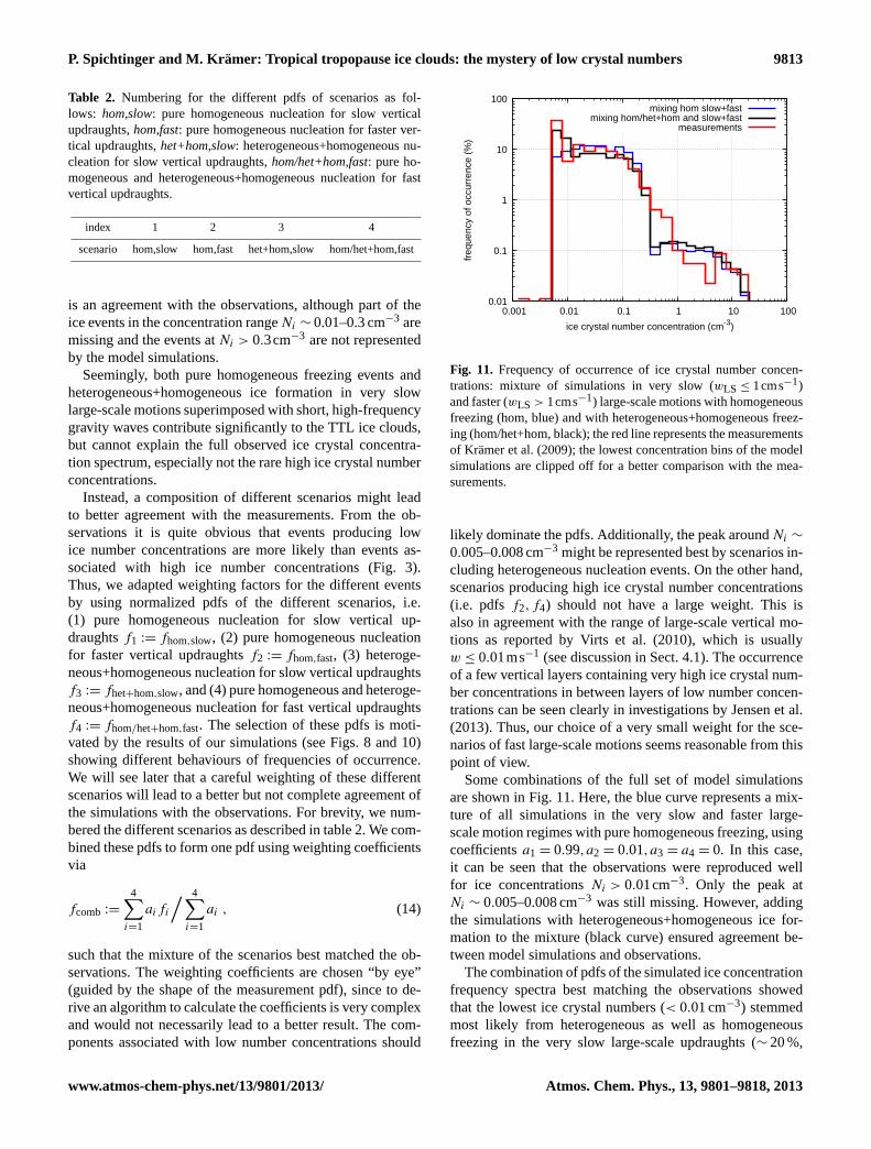
Fig. 11. Frequency of occurrence of ice crystal number concen-trations: mixture of simulations in very slow (wLS ≤ 1cms−1)and faster (wLS > 1cms−1) large-scale motions with homogeneousfreezing (hom, blue) and with heterogeneous+homogeneous freez-ing (hom/het+hom, black); the red line represents the measurementsof Krämer et al.(2009); the lowest concentration bins of the modelsimulations are clipped off for a better comparison with the mea-surements.
likely dominate the pdfs. Additionally, the peak aroundNi ∼
0.005–0.008 cm−3 might be represented best by scenarios in-cluding heterogeneous nucleation events. On the other hand,scenarios producing high ice crystal number concentrations(i.e. pdfs f2,f4) should not have a large weight. This isalso in agreement with the range of large-scale vertical mo-tions as reported byVirts et al. (2010), which is usuallyw ≤ 0.01ms−1 (see discussion in Sect.4.1). The occurrenceof a few vertical layers containing very high ice crystal num-ber concentrations in between layers of low number concen-trations can be seen clearly in investigations byJensen et al.(2013). Thus, our choice of a very small weight for the sce-narios of fast large-scale motions seems reasonable from thispoint of view.
Some combinations of the full set of model simulationsare shown in Fig.11. Here, the blue curve represents a mix-ture of all simulations in the very slow and faster large-scale motion regimes with pure homogeneous freezing, usingcoefficientsa1 = 0.99,a2 = 0.01,a3 = a4 = 0. In this case,it can be seen that the observations were reproduced wellfor ice concentrationsNi > 0.01cm−3. Only the peak atNi ∼ 0.005–0.008 cm−3 was still missing. However, addingthe simulations with heterogeneous+homogeneous ice for-mation to the mixture (black curve) ensured agreement be-tween model simulations and observations.
The combination of pdfs of the simulated ice concentrationfrequency spectra best matching the observations showedthat the lowest ice crystal numbers (< 0.01 cm−3) stemmedmost likely from heterogeneous as well as homogeneousfreezing in the very slow large-scale updraughts (∼ 20 %,
www.atmos-chem-phys.net/13/9801/2013/ Atmos. Chem. Phys., 13, 9801–9818, 2013
9814 P. Spichtinger and M. Krämer: Tropical tropopause ice clouds: the mystery of low crystal numbers
i.e. a3 = 0.2), that the middle ice crystal numbers (0.01–0.3 cm−3) were solely from homogeneous freezing in thesame updraught regime (∼ 79 %, i.e.a1 = 0.79), and thatthe highest TTL ice crystal concentrations (> 0.3 cm−3) alsoevolved from homogeneous freezing or even heterogeneousand homogeneous freezing occurring within the same envi-ronment, but in the faster large-scale updraughts (∼ 1 %, i.e.a4 = 0.01). Consequently, we also seta2 = 0. Hence, about80 % of the TTL cirrus can be explained by “classical” homo-geneous ice nucleation (Koop et al., 2000) and the remaining20 % by a combination of heterogeneous and homogeneousfreezing within the same environment. The mechanism limit-ing the ice crystal production from homogeneous freezing inan environment full of gravity waves is the shortness of thewaves, causing the freezing events to stall before a highernumber of ice crystals can be formed. As stated above, thesuperposition of two different dynamic motion regimes (slowlarge-scale component and high-frequency waves) is crucialfor this kind of mechanism explaining low ice crystal numberconcentrations.
It might be that from superposition of high-frequencywaves nucleation events producing high number concentra-tions are triggered; thus, the weight for the componentf4cannot really be determined, it could be even smaller than1 %. The robust feature, however, is the high frequency ofoccurrence of scenarios with slow large-scale updraughts incombination with high-frequency waves.
6 Discussion
The model study presented here shows that the measured lowTTL ice crystal number concentrations can be representedusing a realistic set-up for the special dynamics in that regionand “classical” homogeneous ice nucleation (e.g.Koop et al.,2000). Additionally, we were able to represent the shape ofthe ice crystal number frequency distribution in a very rea-sonable way.
It was found that the ice crystal number densities arebound to the velocity regimes in the TTL. Superimposing theTTL high-frequency short waves with slow large-scale ver-tical velocities (wLS ≤ 0.01ms−1) yielded the observed lowice crystal number concentrations, since the ice nucleationevents were stalled early on by downdraughts. On the otherhand, lower frequencies of the short gravity waves or fasterlarge-scale motions (wLS > 0.01ms−1) triggered higher icecrystal number concentrations. These cases reflect what wewould expect from theory (Lin et al., 1998; Hoyle et al.,2005) and what is usually discussed in studies about the im-pact of homogeneous nucleation on the TTL ice crystal num-bers, concluding that this formation mechanism is unable toproduce low ice concentrations (Jensen and Pfister, 2004).The major new part of our study is the special combination ofhigh frequency wavesandvery slow large-scale updraughts.
Furthermore, we found that the shape of the measured icecrystal frequency distribution can be represented by mixingdifferent possible scenarios: in many cases there were noheterogeneous IN available, and thus pure homogeneous nu-cleation was the dominant pathway (∼ 79 %). In some rarerscenarios, heterogeneous nucleation took place in additionto homogeneous nucleation (∼ 20 %), and finally, sometimesthe dynamic conditions also differed, i.e. the more unlikelycase of faster large-scale updraughts occurred (∼ 1 %). Gen-erally, we can state that heterogeneous nucleation is not themain pathway for the formation of very low ice crystal num-ber concentrations, but that the major mechanism is homo-geneous ice nucleation driven by the special TTL dynam-ics; heterogeneous nucleation simply modifies the nucleationevents but does not qualitatively change the results.
In many recent studies (see e.g.Murray et al., 2010) thecontamination of the sulfuric acid droplets by organics andthus the inhibition of homogeneous nucleation is consideredto be the main reason for very low ice crystal number con-centrations in the TTL. However, homogeneous nucleationwould only be suppressed, if almost all background aerosoldroplets were contaminated by these substances. From re-cent measurements (see e.g.Froyd et al., 2009), we knowthat there is a significant contribution of organics in the TTL.However, the relative mass fraction of organics in the TTLis never higher than 80 % (e.g. the case of Pre-AVE1, whereexceptionally high values were measured), and in many mea-surements, the relative fraction of organics in the TTL is inthe range of 0.1–0.5 (e.g. CR-AVE2 cases). Thus, it is veryunlikely – at least from real measurements – that organicscan suppress homogeneous nucleation completely, since thenon-contaminated particles will nucleate to ice crystals.
In former studies on the impact of dynamics, a spectrum ofgravity waves was usually used to drive the box models (seee.g.Jensen and Pfister, 2004). Although these spectra weredetermined from measurements, it is unclear if they are re-ally representative of the TTL conditions and high-frequencywaves were not included in these studies. The main reasonfor neglecting these waves was the lack of measurement tech-niques capable of detecting these very short wavelengths orequivalently high frequencies. Thus, the effects discussed inthis study were not included in former studies. As we pointedout in our discussion, the short wavelengths (i.e. high fre-quenciesω > 0.005s−1) are extremely important for veryshort freezing events. For longer wavelengths (i.e. low fre-quenciesω < 0.005s−1), as used in former studies, the im-pact of dynamics increases significantly the ice crystal num-ber concentrations.
In our study, we concentrated on monochromatic waves,which is a reasonable restriction. However, if we wereto assume a spectrum of superimposed waves within thenarrow spectral window as indicated by the theoretical
1Pre-Aura Validation Experiment, 20042Costa Rica Aura Validation Experiment, 2006
Atmos. Chem. Phys., 13, 9801–9818, 2013 www.atmos-chem-phys.net/13/9801/2013/
P. Spichtinger and M. Krämer: Tropical tropopause ice clouds: the mystery of low crystal numbers 9815
considerations (Ruprecht et al., 2010), this might lead to aspread in number concentrations towards larger values. Insome sensitivity studies (not shown), the quality of the re-sults driven by monochromatic waves did not change.
In contrast to former studies (see e.g.Jensen and Pfister,2004; Jensen et al., 2010) the amplitude of the waves wasnot restricted to very small amplitudes to obtain low ice crys-tal number concentrations. For our approach this restrictionwas unnecessary, because the nucleation event was deter-mined by the high frequencies (ω ∈ [0.005s−1
: 0.029s−1])
and not by the amplitude of the waves. Thus, our simulationswere more realistic in this sense, because the whole spreadof amplitudes in the range up to1T ∼ 1 K can be observedfrom measurements (Gary, 2006). Our results are in qualita-tive agreement with former studies byBarahona and Nenes(2011) for their investigations with temperature amplitudesδT ≤ 1 K although we had a different approach where weused high-frequency waves.
With the box model approach mixing effects cannot betaken into account. Actually, there are two effects whichmight influence the formation of ice crystals. First, horizon-tal motions could lead to a spread of formed ice crystals intoneighbouring regions where ice nucleation did not occur be-fore. Thus, the spread crystals will then grow in supersatu-rated but clear air, reducing water vapour such that further icenucleation is quenched. This effect was already investigatedin former studies (Spichtinger and Gierens, 2009b). Second,ice crystals from ice clouds above (e.g. from convective out-flow or in situ formed clouds) could sediment into clear airand again quench ice nucleation, as discussed in former stud-ies (Barahona and Nenes, 2011). Both effects would lead toa further reduction of ice crystal number concentrations in-stead of an enhancement.
We already mentioned the contamination of the back-ground aerosol solution droplets by organic substances. Al-though the contamination and thus suppression of homoge-neous nucleation works well in laboratory experiments (Zo-brist et al., 2008; Murray et al., 2010), at the moment there isno indication from in situ measurements in the TTL (a) thatthe respective substances (e.g. citric acid) are available in theTTL and (b) that there is contamination of almost all aerosolparticles in order to guarantee total suppression of homoge-neous nucleation (see e.g. discussion inKärcher and Koop,2005). The corroboration by measurements is still lacking.On the other hand, contamination of some aerosol particlescould lead to additional heterogeneous IN. Since we did notspecify the type of heterogeneous INs used in this study,there could be room for such glassy particles.
However, in our opinion, the total suppression of homoge-neous nucleation by contamination with the suitable materialis the subject of a very complex theory. Our proposal allowsclassical homogeneous and heterogeneous ice nucleation tooccur in a very simple dynamic set-up, given by the specialenvironment of the TTL. Applying Ockham’s razor (princi-ple of parsimony) we tend to prefer the simpler dynamic ap-
proach, particularly because our simulations show very goodagreement with in situ measurements.
7 Conclusions
In summary, we showed that the superposition of high-frequency internal gravity waves with very slow large-scalemotions (e.g. driven by Kelvin waves) could trigger homo-geneous freezing events in such a way that the low ice crys-tal number concentrations measured in the TTL are reason-ably represented:∼ 79 % of the ice crystals were formedby “classical” homogeneous freezing in very-slow large-scale motions,∼ 20 % stemmed from combined heteroge-neous+homogeneous ice nucleation in very slow large-scalemotions, and only∼ 1 % came from homogeneous freezingwith or without simultaneously occurring heterogeneous nu-cleation in faster large-scale motions. It might be that ourresults are too simplified in terms of neglecting the superpo-sition of many different wave components, leading to higherconcentrations. However, the signature of low crystal numberconcentrations stemming from slow large-scale motions su-perimposed by high-frequency waves is a robust signal fromour investigations.
There is, therefore, an interplay of the different comple-mentary mechanisms (e.g. TTL dynamics, homogeneous andheterogeneous ice nucleation, as well as the suppression ofnucleation by organic substances or crystallization of ammo-nium sulfate) which may lead to the phenomenon of low icecrystal number concentrations. In order to verify the rela-tive contributions of these different effects, more measure-ments in the TTL are necessary. To investigate these effectsin a more general treatment, additional two- or even three-dimensional model simulations including a realistic treat-ment of gravity waves are important.
Finally, we want to remark that for producing low ice crys-tal number concentrations correctly in large-scale models, itmight be reasonable to switch off the subgrid scale verticalvelocities and to trigger nucleation exclusively by large-scalemotions in the TTL. Our results suggest that this approachwould likely lead to more reasonable ice crystal number con-centrations in the TTL for general circulation models as usedfor climate studies.
Appendix A
Equations (7) and (10) describe the time evolution of tem-perature and vertical velocity, respectively. The amplitudesfor the wave components for temperatureAT and vertical ve-locity Aw are related via the intrinsic frequency of the waveω =
2πτ
, i.e.
Aw =cp
gω · AT . (A1)
www.atmos-chem-phys.net/13/9801/2013/ Atmos. Chem. Phys., 13, 9801–9818, 2013
9816 P. Spichtinger and M. Krämer: Tropical tropopause ice clouds: the mystery of low crystal numbers
Table A1. Intrinsic frequenciesN = f · Nmax, periodsτ =2πN
and
vertical velocity amplitudesAw =cp
g N · AT for different stabilityregimesNmax using a temperature amplitude ofAT = 1 K.
Nmax= 0.029s−1
f N (s−1) τ (s) Aw (ms−1)
0.4 0.011600 541.654 1.18800.6 0.017400 361.103 1.78200.8 0.023200 270.827 2.37611.0 0.029000 216.662 2.9701
Nmax= 0.022s−1
f N (s−1) τ (s) Aw (ms−1)
0.4 0.008800 713.998 0.90130.6 0.013200 475.999 1.35190.8 0.017600 356.999 1.80251.0 0.022000 285.599 2.2532
Nmax= 0.0172s−1
f N (s−1) τ (s) Aw (ms−1)
0.4 0.006880 913.254 0.70460.6 0.010320 608.836 1.05690.8 0.013760 456.627 1.40921.0 0.017200 365.301 1.7616
Nmax= 0.0128s−1
f N (s−1) τ (s) Aw (ms−1)
0.4 0.005120 1227.185 0.52440.6 0.007680 818.123 0.78660.8 0.010240 613.592 1.04871.0 0.012800 490.874 1.3109
In TableA1 the values ofω = N = f · Nmax, τ andAw, re-spectively, are shown for the realistic set-up as described inSect.5.1 for values off = 0.4/0.6/0.8/1.0. Here, we as-sume a temperature amplitude ofAT = 1 K.
Similarly, the vertical displacementz(t) can be describedby integrating the equationdz
dt= w(t) via separation of vari-
ables, leading to the following expression:
z(t) − z0 = wLS · t −Aw
ω· cos(ωt)
= wLS · t −cp
gAT︸ ︷︷ ︸
:=Az
·cos(ωt). (A2)
For values ofAT = 0.1/0.25/0.5/0.75/1.0 K in the realisticset-up in Sect.5.1the maximal displacement in terms of am-plitudesAz is displayed in TableA2.
Table A2. Amplitudes of temperatureAT, and vertical displace-mentAz, respectively.
AT (K) 0.1 0.25 0.5 0.75 1.0
Az (m) 10.24 25.60 51.21 76.81 102.42
Acknowledgements.We would like to thank Stephan Borrmannfor providing the ice crystal data and Klaus Gierens, Ben Murray,Riwal Plougonven and Holger Tost for fruitful discussions. Wealso greatly acknowledge Hazel Burlet from the Language Serviceof the Research Center Jülich for improving the English languageof the manuscript. The output from the aerosol model was kindlyprovided by Debra Weisenstein and Ana Cirisan. This studycontributes to the COST action Atmospheric Water Vapour in theClimate System (WaVaCS).
Edited by: W. Lahoz
This publication is supportedby COST –www.cost.eu
References
Barahona, D. and Nenes, A. : Parameterization of cirrus cloud for-mation in large-scale models: Homogeneous nucleation, J. Geo-phys. Res., 113, D11211, doi:10.1029/2007JD009355, 2008.
Barahona, D. and Nenes, A.: Dynamical states of low temperaturecirrus. Atmos. Chem. Phys., 11, 3757–3771, doi:10.5194/acp-11-3757-2011, 2011.
Boehm, M. D. and Verlinde, J.: Stratospheric influence on uppertropospheric tropical cirrus, Geophys. Res. Lett., 27, 3209–3212,2000.
Bretherton, C. S. and Smolarkiewicz, P. K.: Gravity waves, com-pensating subsidence and detrainment around cumulus clouds, J.Atmos. Sci., 46, 740–759, 1989.
DeMott, P., Cziczo, D., Prenni, A., Murphy, D., Kreidenweis, S.,Thomson, D., Borys, R., and Rogers, D.: Measurements of theconcentration and composition of nuclei for cirrus formation, P.Natl. Acad. Sci., 100, 14655–14660, 2003.
Flury, T., Wu, D. L., and Read, W. G.: Correlation among cirrus icecontent, water vapor and temperature in the TTL as observed byCALIPSO and Aura/MLS, Atmos. Chem. Phys., 12, 683–691,doi:10.5194/acp-12-683-2012, 2012.
Forster, P. M. and Shine, K. P.: Assessing the climate impact oftrends in stratospheric water vapor, Geophys. Res. Lett., 29,1086, doi:10.1029/2001GL013909, 2002.
Fueglistaler, S., Dessler, A. E., Dunkerton, T. J., Folkins, I., Fu, Q.,and Mote, P. W.: Tropical Tropopause Layer, Rev. Geophys., 47,RG1004, doi:10.1029/2008RG000267, 2009a.
Fueglistaler, S., Legras, B., Beljaars, A., Morcrette, J.-J., Simmons,A., Tompkins, A. M., and Uppala, S.: The diabatic heat budgetof the upper troposphere and lower/mid stratosphere in ECMWFreanalyses, Q. J. Roy. Meteor. Soc., 135, 21–37, 2009b.
Froyd, K. D., Murphy, D. M., Sanford, T. J., Thomson, D. S., Wil-son, J. C., Pfister, L., and Lait, L.: Aerosol composition of the
Atmos. Chem. Phys., 13, 9801–9818, 2013 www.atmos-chem-phys.net/13/9801/2013/
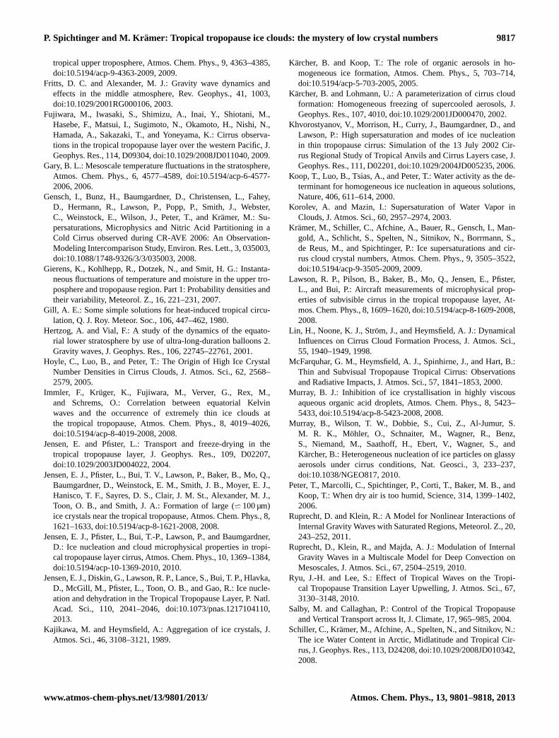
P. Spichtinger and M. Krämer: Tropical tropopause ice clouds: the mystery of low crystal numbers 9817
tropical upper troposphere, Atmos. Chem. Phys., 9, 4363–4385,doi:10.5194/acp-9-4363-2009, 2009.
Fritts, D. C. and Alexander, M. J.: Gravity wave dynamics andeffects in the middle atmosphere, Rev. Geophys., 41, 1003,doi:10.1029/2001RG000106, 2003.
Fujiwara, M., Iwasaki, S., Shimizu, A., Inai, Y., Shiotani, M.,Hasebe, F., Matsui, I., Sugimoto, N., Okamoto, H., Nishi, N.,Hamada, A., Sakazaki, T., and Yoneyama, K.: Cirrus observa-tions in the tropical tropopause layer over the western Pacific, J.Geophys. Res., 114, D09304, doi:10.1029/2008JD011040, 2009.
Gary, B. L.: Mesoscale temperature fluctuations in the stratosphere,Atmos. Chem. Phys., 6, 4577–4589, doi:10.5194/acp-6-4577-2006, 2006.
Gensch, I., Bunz, H., Baumgardner, D., Christensen, L., Fahey,D., Hermann, R., Lawson, P., Popp, P., Smith, J., Webster,C., Weinstock, E., Wilson, J., Peter, T., and Krämer, M.: Su-persaturations, Microphysics and Nitric Acid Partitioning in aCold Cirrus observed during CR-AVE 2006: An Observation-Modeling Intercomparison Study, Environ. Res. Lett., 3, 035003,doi:10.1088/1748-9326/3/3/035003, 2008.
Gierens, K., Kohlhepp, R., Dotzek, N., and Smit, H. G.: Instanta-neous fluctuations of temperature and moisture in the upper tro-posphere and tropopause region. Part 1: Probability densities andtheir variability, Meteorol. Z., 16, 221–231, 2007.
Gill, A. E.: Some simple solutions for heat-induced tropical circu-lation, Q. J. Roy. Meteor. Soc., 106, 447–462, 1980.
Hertzog, A. and Vial, F.: A study of the dynamics of the equato-rial lower stratosphere by use of ultra-long-duration balloons 2.Gravity waves, J. Geophys. Res., 106, 22745–22761, 2001.
Hoyle, C., Luo, B., and Peter, T.: The Origin of High Ice CrystalNumber Densities in Cirrus Clouds, J. Atmos. Sci., 62, 2568–2579, 2005.
Immler, F., Krüger, K., Fujiwara, M., Verver, G., Rex, M.,and Schrems, O.: Correlation between equatorial Kelvinwaves and the occurrence of extremely thin ice clouds atthe tropical tropopause, Atmos. Chem. Phys., 8, 4019–4026,doi:10.5194/acp-8-4019-2008, 2008.
Jensen, E. and Pfister, L.: Transport and freeze-drying in thetropical tropopause layer, J. Geophys. Res., 109, D02207,doi:10.1029/2003JD004022, 2004.
Jensen, E. J., Pfister, L., Bui, T. V., Lawson, P., Baker, B., Mo, Q.,Baumgardner, D., Weinstock, E. M., Smith, J. B., Moyer, E. J.,Hanisco, T. F., Sayres, D. S., Clair, J. M. St., Alexander, M. J.,Toon, O. B., and Smith, J. A.: Formation of large (w 100 µm)ice crystals near the tropical tropopause, Atmos. Chem. Phys., 8,1621–1633, doi:10.5194/acp-8-1621-2008, 2008.
Jensen, E. J., Pfister, L., Bui, T.-P., Lawson, P., and Baumgardner,D.: Ice nucleation and cloud microphysical properties in tropi-cal tropopause layer cirrus, Atmos. Chem. Phys., 10, 1369–1384,doi:10.5194/acp-10-1369-2010, 2010.
Jensen, E. J., Diskin, G., Lawson, R. P., Lance, S., Bui, T. P., Hlavka,D., McGill, M., Pfister, L., Toon, O. B., and Gao, R.: Ice nucle-ation and dehydration in the Tropical Tropopause Layer, P. Natl.Acad. Sci., 110, 2041–2046, doi:10.1073/pnas.1217104110,2013.
Kajikawa, M. and Heymsfield, A.: Aggregation of ice crystals, J.Atmos. Sci., 46, 3108–3121, 1989.
Kärcher, B. and Koop, T.: The role of organic aerosols in ho-mogeneous ice formation, Atmos. Chem. Phys., 5, 703–714,doi:10.5194/acp-5-703-2005, 2005.
Kärcher, B. and Lohmann, U.: A parameterization of cirrus cloudformation: Homogeneous freezing of supercooled aerosols, J.Geophys. Res., 107, 4010, doi:10.1029/2001JD000470, 2002.
Khvorostyanov, V., Morrison, H., Curry, J., Baumgardner, D., andLawson, P.: High supersaturation and modes of ice nucleationin thin tropopause cirrus: Simulation of the 13 July 2002 Cir-rus Regional Study of Tropical Anvils and Cirrus Layers case, J.Geophys. Res., 111, D02201, doi:10.1029/2004JD005235, 2006.
Koop, T., Luo, B., Tsias, A., and Peter, T.: Water activity as the de-terminant for homogeneous ice nucleation in aqueous solutions,Nature, 406, 611–614, 2000.
Korolev, A. and Mazin, I.: Supersaturation of Water Vapor inClouds, J. Atmos. Sci., 60, 2957–2974, 2003.
Krämer, M., Schiller, C., Afchine, A., Bauer, R., Gensch, I., Man-gold, A., Schlicht, S., Spelten, N., Sitnikov, N., Borrmann, S.,de Reus, M., and Spichtinger, P.: Ice supersaturations and cir-rus cloud crystal numbers, Atmos. Chem. Phys., 9, 3505–3522,doi:10.5194/acp-9-3505-2009, 2009.
Lawson, R. P., Pilson, B., Baker, B., Mo, Q., Jensen, E., Pfister,L., and Bui, P.: Aircraft measurements of microphysical prop-erties of subvisible cirrus in the tropical tropopause layer, At-mos. Chem. Phys., 8, 1609–1620, doi:10.5194/acp-8-1609-2008,2008.
Lin, H., Noone, K. J., Ström, J., and Heymsfield, A. J.: DynamicalInfluences on Cirrus Cloud Formation Process, J. Atmos. Sci.,55, 1940–1949, 1998.
McFarquhar, G. M., Heymsfield, A. J., Spinhirne, J., and Hart, B.:Thin and Subvisual Tropopause Tropical Cirrus: Observationsand Radiative Impacts, J. Atmos. Sci., 57, 1841–1853, 2000.
Murray, B. J.: Inhibition of ice crystallisation in highly viscousaqueous organic acid droplets, Atmos. Chem. Phys., 8, 5423–5433, doi:10.5194/acp-8-5423-2008, 2008.
Murray, B., Wilson, T. W., Dobbie, S., Cui, Z., Al-Jumur, S.M. R. K., Möhler, O., Schnaiter, M., Wagner, R., Benz,S., Niemand, M., Saathoff, H., Ebert, V., Wagner, S., andKärcher, B.: Heterogeneous nucleation of ice particles on glassyaerosols under cirrus conditions, Nat. Geosci., 3, 233–237,doi:10.1038/NGEO817, 2010.
Peter, T., Marcolli, C., Spichtinger, P., Corti, T., Baker, M. B., andKoop, T.: When dry air is too humid, Science, 314, 1399–1402,2006.
Ruprecht, D. and Klein, R.: A Model for Nonlinear Interactions ofInternal Gravity Waves with Saturated Regions, Meteorol. Z., 20,243–252, 2011.
Ruprecht, D., Klein, R., and Majda, A. J.: Modulation of InternalGravity Waves in a Multiscale Model for Deep Convection onMesoscales, J. Atmos. Sci., 67, 2504–2519, 2010.
Ryu, J.-H. and Lee, S.: Effect of Tropical Waves on the Tropi-cal Tropopause Transition Layer Upwelling, J. Atmos. Sci., 67,3130–3148, 2010.
Salby, M. and Callaghan, P.: Control of the Tropical Tropopauseand Vertical Transport across It, J. Climate, 17, 965–985, 2004.
Schiller, C., Krämer, M., Afchine, A., Spelten, N., and Sitnikov, N.:The ice Water Content in Arctic, Midlatitude and Tropical Cir-rus, J. Geophys. Res., 113, D24208, doi:10.1029/2008JD010342,2008.
www.atmos-chem-phys.net/13/9801/2013/ Atmos. Chem. Phys., 13, 9801–9818, 2013
9818 P. Spichtinger and M. Krämer: Tropical tropopause ice clouds: the mystery of low crystal numbers
Seifert, A. and Beheng, K. D.: : A two-moment cloud microphysicsparameterization for mixed-phase clouds. Part 1: Model descrip-tion, Meteorol. Atmos. Phys., 92, 45–66, 2006.
Selkirk, H. B., Vömel, H., Valverde Canossa, J. M., Pfister, L.,Diaz, J. A., Fernández, W., Amador, J., Stolz, W., and Peng,G. S.: Detailed structure of the tropical upper troposphere andlower stratosphere as revealed by balloon sonde observations ofwater vapor, ozone, temperature, and winds during the NASATCSP and TC4 campaigns, J. Geophys. Res., 115, D00J19,doi:10.1029/2009JD013209, 2010.
Spichtinger, P. and Cziczo, D. J.: Impact of heterogeneous ice nucleion homogeneous freezing events in cirrus clouds, J. Geophys.Res., 15, D14208, doi:10.1029/2009JD012168, 2010.
Spichtinger, P. and Gierens, K. M.: Modelling of cirrus clouds –Part 1a: Model description and validation, Atmos. Chem. Phys.,9, 685–706, doi:10.5194/acp-9-685-2009, 2009a.
Spichtinger, P. and Gierens, K. M.: Modelling of cirrus clouds – Part1b: Structuring cirrus clouds by dynamics, Atmos. Chem. Phys.,9, 707–719, doi:10.5194/acp-9-707-2009, 2009b.
Spichtinger, P. and Gierens, K. M.: Modelling of cirrus clouds– Part 2: Competition of different nucleation mechanisms, At-mos. Chem. Phys., 9, 2319–2334, doi:10.5194/acp-9-2319-2009,2009c.
Thomas, A., Borrmann, S., Kiemle, C., Cairo, F., Volk, M., Beuer-mann, J., Lepuchov, B., Santacesaria, V., Matthey, R., Rudakov,V., Yushkov, V., MacKenzie, A. R., and Stefanutti, L.: In situmeasurements of background aerosol and subvisible cirrus inthe tropical tropopause region, J. Geophys. Res., 107, 4763,doi:10.1029/2001JD001385, 2002.
Thompson, A. M., Witte, J. C., McPeters, R. D., Oltmans, S. J.,Schmidlin, F. J., Logan, J. A., Fujiwara, M., Kirchhoff, V. W.J. H., Posny, F., Coetzee, G. J. R., Hoegger, B., Kawakami, S.,Ogawa, T., Johnson, B. J., Vömel, H., and Labow, G.: SouthernHemisphere Additional Ozonesondes (SHADOZ) 1998–2000tropical ozone climatology 1. Comparison with Total OzoneMapping Spectrometer (TOMS) and ground-based measure-ments, J. Geophys. Res., 108, 8238, doi:10.1029/2001JD000967,2003.
Thompson, A. M., Allen, A. L., Lee, S., Miller, S. K., and Witte,J. C.: Gravity and Rossby wave signatures in the tropical tro-posphere and lower stratosphere based on Southern HemisphereAdditional Ozonesondes (SHADOZ), 1998–2007, J. Geophys.Res., 116, D05302, doi:10.1029/2009JD013429, 2011.
Vial, F., Hertzog, A., Mechoso, C. R., Basdevant, C., Cocquerez, P.,Dubourg, V., and Nouel, F.: A study of the dynamics of the equa-torial lower stratosphere by use of ultra-long-duration balloons,1. Planetary scales, J. Geophys. Res., 106, 22725–22743, 2001.
Virts, K.: Cirrus in the Tropical Tropopause Transition Layer: For-mation Mechanisms and Influence of the Local and Planetary-Scale Environment, MSc thesis, University of Washington,108 pp., available at:http://www.atmos.washington.edu/~kvirts/docs/Thesis.pdf, 2009
Virts, K., Wallace, J., Fu, Q., and Ackermann, T.: Tropi-cal Tropopause Transition Layer Cirrus as Represented byCALIPSO Lidar Observations, J. Atmos. Sci., 67, 3113–3129,2010.
Wang, L., Alexander, M. J., Bui, T. B., and Mahoney, M. J.: Small-scale gravity waves in ER-2 MMS/MTP wind and temperaturemeasurements during CRYSTAL-FACE, Atmos. Chem. Phys., 6,1091–1104, doi:10.5194/acp-6-1091-2006, 2006.
Webster, P. J.: Response of the tropical atmosphere to local, steadyforcing, Mon. Weather Rev., 100, 518–541, 1972.
Weisenstein, D. K., Penner, J. E., Herzog, M., and Liu, X.: Global 2-D intercomparison of sectional and modal aerosol modules, At-mos. Chem. Phys., 7, 2339–2355, doi:10.5194/acp-7-2339-2007,2007.
Wheeler, M., Kiladis, G. N., and Webster, P. J.: Large-scale dynami-cal fields associated with convectively coupled equatorial waves,J. Atmos. Sci., 57, 613–640, 2000.
Zobrist, B., Marcolli, C., Pedernera, D. A., and Koop, T.: Do atmo-spheric aerosols form glasses?, Atmos. Chem. Phys., 8, 5221–5244, doi:10.5194/acp-8-5221-2008, 2008.
Atmos. Chem. Phys., 13, 9801–9818, 2013 www.atmos-chem-phys.net/13/9801/2013/