trend inflation in advanced economies - ijcb · trend inflation in advanced economies ... sargent...
TRANSCRIPT

Trend Inflation in Advanced Economies∗
Christine Garnier,a Elmar Mertens,b and Edward Nelsonc
aTufts UniversitybFederal Reserve BoardcUniversity of Sydney
We derive estimates of trend inflation for fourteen advancedeconomies from a framework in which trend shocks exhibit sto-chastic volatility. The estimated specification allows for timevariation in the degree to which longer-term inflation expecta-tions are well anchored in each economy. Our results bring outthe effect of changes in monetary regime (such as the adoptionof inflation targeting in several countries) on the behavior oftrend inflation.
Our estimates represent an expansion of those in the pre-vious literature along several dimensions. For each country, weemploy a multivariate approach that pools different inflationseries in order to identify their common trend. In addition, ourestimates of the inflation gap (that is, the difference betweentrend and observed inflation) are allowed to exhibit consider-able persistence—a treatment that affects the trend estimatesto some extent. A forecast evaluation based on quasi-real-timeestimates registers sizable improvements in inflation forecasts
∗We would like to thank our discussant, James Morley, and participants inthe Reserve Bank of New Zealand/International Journal of Central Bankingresearch conference, “Reflections on 25 Years of Inflation Targeting,” hosted bythe Reserve Bank of New Zealand on December 1–2, 2014, for their very usefulcomments and suggestions. We are also grateful for feedback received at the Fed-eral Reserve System Committee on International Economic Analysis conferenceof May 2013, held at the Federal Reserve Board, including the valuable remarksof our discussant, Jonathan Wright, as well as for comments of participants ina seminar at the University of Sydney in August 2014. We are also indebted toConefrey Thomas and Stefan Gerlach for providing us with price-level data forIreland and to Will Gamber for research assistance. The views in this paper do notnecessarily represent those of the Federal Reserve Board, or any other person inthe Federal Reserve System or the Federal Open Market Committee. Any errorsor omissions should be regarded as solely those of the authors. Correspondingauthor (Mertens) e-mail: [email protected].
65

66 International Journal of Central Banking September 2015
at different horizons for almost all countries considered. Itremains the case, however, that simple random-walk forecastsof inflation are difficult to outperform by a statistically signif-icant amount.
JEL Codes: C53, E37, E47, E58.
1. Introduction
Measures of trend inflation play an important role in the study ofinflation in many countries. In the context of policy analysis, thelevel and variability of trend inflation can be viewed as summariesof the degree to which inflation expectations in a particular countryhave remained anchored over time. Application of New Keynesiananalysis to inflation data over long samples may also benefit fromthe availability of estimates of trend inflation, as the New Keynesianapproach to the Phillips curve typically specifies inflation dynamicsin terms of the deviation of inflation from a steady-state or trend-inflation rate, with this trend rate possibly varying over time (see, forexample, Cogley and Sbordone 2008). Furthermore, an estimate oftrend inflation can serve as a useful centering point in the construc-tion of inflation forecasts at various horizons. Still another reason forinterest in estimates of trend inflation is the fact that the existingliterature has found that a substantial portion of the observed per-sistence of international inflation data is accounted for by variationsin trend inflation, which are in turn often related to changes in mon-etary regimes; see, for example, Levin and Piger (2004), Cecchettiet al. (2007), Ireland (2007), Stock and Watson (2007, 2010), Wright(2011), and Morley, Piger, and Rasche (2015).
In this paper, we provide estimates of the level of, andtime-varying uncertainty of, trend inflation for fourteen advancedeconomies. The estimates are derived from a multivariate statisticalmodel that pools information from different inflation series for eachcountry. The model is applied on a country-by-country basis.1 Ourmotivation for this choice is twofold. First, the country-by-countryapproach is most amenable to a comparison, for the full sample
1This approach contrasts with the procedure of pooling information acrosscountries, as in Mumtaz and Surico (2009, 2012), Ciccarelli and Mojon (2010),and Mumtaz, Simonelli, and Surico (2011), for example.

Vol. 11 No. S1 Trend Inflation in Advanced Economies 67
period as well as for subsamples, of alternative models of trend. Sec-ond, although there are clearly some cross-country co-movementsin overall inflation, the reason that inflation rates move togetheracross countries does not appear to lie solely in common behaviorof the trend component of a “trend/cycle” decomposition—a com-plication that is underscored in, for example, Ciccarelli and Mojon’s(2010) analysis of cross-country inflation behavior. On this score,our results confirm that there do, in fact, tend to be considerabledifferences across countries in estimates of trend inflation, very likelyreflecting country-specific developments in monetary regimes.
Formally, we adopt the definition of trend inflation as the infinite-horizon forecast of inflation. This trend definition corresponds tothe Beveridge-Nelson (1981) concept. This concept has been appliedto inflation data in a number of studies, including Cecchetti etal. (2007), Stock and Watson (2007, 2010), Clark and Doh (2011),Cogley, Sargent, and Surico (2014), Cogley and Sargent (2015), andMorley, Piger, and Rasche (2015), with variants of the approachalso employed by Cogley and Sargent (2005), Cogley, Primiceri, andSargent (2010), and Kozicki and Tinsley (2012).2 Our multivariatemodel incorporates the assumption that, for any particular country,different inflation measures share the same common trend. Specifi-cally, we consider percentage changes in core and headline CPI, aswell as percentage changes in the GDP deflator, proceeding through-out on the premise that the deviations that these inflation seriesexhibit from the common trend are dynamically stable.
Our multivariate model, designated the “MVSV” model, neststhe popular unobserved-components model with stochastic volatil-ity, designated the “UCSV” model, of Stock and Watson (2007,2010) that has been applied to inflation data for the G7 countries byCecchetti et al. (2007). The application of a multivariate extension ofthe UCSV model to different countries, and the comparison betweenUCSV and MVSV models across these economies, constitute specific
2Cogley and Sargent (2005) and Cogley, Primiceri, and Sargent (2010) derivetheir measure of trend inflation from a non-linear function of time-varying VARcoefficients, a measure that approximately corresponds to a Beveridge-Nelson(1981) trend. Kozicki and Tinsley (2012) refer to their measure as the “shiftingendpoint of inflation expectations.” In a similar spirit, Levin and Piger (2004)relate time variation in inflation persistence to structural breaks in the coefficientsof autoregressive time-series representations of inflation.

68 International Journal of Central Banking September 2015
contributions of this paper. The multivariate model used in thispaper represents an extension of the UCSV approach along twodimensions. The first dimension pertains to our reliance on multipleinflation series: as in Mertens (2011), the model extracts its trendestimates from a set of inflation series, instead of drawing infor-mation from a single inflation measure. The second dimension per-tains to the treatment of the difference between trend and observedinflation—the inflation gap, in the terminology of Cogley, Primiceri,and Sargent (2010). Inflation-gap fluctuations are assumed to beserially uncorrelated in the UCSV model. In contrast, we allow theinflation gap to exhibit considerable persistence, while constrainingthe gap fluctuations to be dynamically stable, governed by a vec-tor autoregression with time-invariant parameters. In this way, weallow for the possibility of persistence in the inflation gap, as in, forexample, Kang, Kim, and Morley (2009) or Cogley, Primiceri, andSargent (2010). Unlike these authors, however, we do not permitinflation-gap persistence to vary over time. The more parsimoniousapproach to the treatment of inflation-gap persistence that we adopthas advantages that we discuss below.
As in the UCSV model, we keep track of different measures ofstochastic volatility that affect different components of the infla-tion process: one for trend shocks and one capturing changes in gapvolatility for each of the different inflation measures used in our mul-tivariate model. Although we allow for time-varying persistence ineach inflation measure by letting the magnitude of shocks to theinflation trend and gap vary, we have also chosen to keep the coeffi-cients governing inflation-gap persistence constant in order to limittime variation in model parameters. Such a restriction is especiallywarranted in view of the fact that we lack observations on severalinput series in the earlier part of our sample.
In the spirit of the UCSV model, our procedure does not involvetaking a stand on the issue of potential statistical linkages betweeninflation and other economic variables. For example, we do not inves-tigate connections between persistent behavior of inflation and per-sistence in resource slack (such as those considered in, for example,Morley, Piger, and Rasche 2015). In so limiting the scope of ouranalysis, we in no way deny that such linkages are of economicinterest. On the contrary, real/nominal interactions are crucial tomonetary policy analysis. But trend estimates of the kind we derive

Vol. 11 No. S1 Trend Inflation in Advanced Economies 69
are closely related to a model’s forecasting properties, and the con-tribution that real variables make to the forecasting of inflation hasfrequently been established to be modest—as documented in, forexample, Stock and Watson (2009) and Faust and Wright (2013).Accordingly, attention is confined here to models of the inflationprocess that do not draw upon data other than on inflation. There-fore, when we speak of our estimates being “multivariate,” we meanthat we use multiple measures of inflation in estimation; we do notuse series other than inflation to inform our estimates.3
Because our estimation relies on state-space methods andinvolves a limited number of time-varying parameters, we can han-dle cases in which observations are missing for particular inflationseries. Throughout our estimation, we use data beginning in 1960.Associated with this early start date for the sample is the fact that,for some countries, subsets of the series used may have missing obser-vations, reflecting a later initial date for those series or other data-availability problems. In addition to providing estimates that takethis data issue into account, we also consider estimates that areconditioned on data sets for which available observations on infla-tion have been discarded for certain dates for judgmental reasons.These reasons reflect our concern that the variations in inflationrecorded in certain periods arose from “price shifts,” with the latterattributable to non-market factors—such as outright governmentalprice controls or tax changes that bore directly on measured infla-tion. In taking this approach regarding price shifts, we expand on anumber of earlier studies, including Gordon (1983), Levin and Piger(2004), Neiss and Nelson (2005), and Morley, Piger, and Rasche(2015), to name only a few.4 In comparing estimates with and with-out allowance for price shifts, we find that the shifts tend to have an
3We believe, however, that the approach to the data we take here has elementsthat could be usefully applied to the study of the inflation/resource slack connec-tion. For example, our concern with controlling for episodes in which price con-trols distorted measured inflation series is highly relevant for the task of obtainingvalid estimates of the inflation trend in a context in which resource-slack seriesare among the variables used in the computation of the trend.
4Cecchetti et al. (2007, p. 14) adjusted their data on real GDP growth forFrance for a strike-affected observation. In so doing, they recognized the princi-ple that disruptions to market activity should not be permitted to affect trendestimates. They did not, however, apply this principle to their estimation of trendinflation.

70 International Journal of Central Banking September 2015
appreciable effect on trend estimates—especially so for the UCSVmodel—a result that suggests that the shift-affected inflation obser-vations should be excluded when estimating trend inflation. On theother hand, our multivariate estimates of the inflation trend showsigns of being more robust to the inclusion of such periods in theestimation.
Finally, we compare the forecast performance of our multi-variate model with that of the UCSV model and (as in Atkesonand Ohanian 2001) random-walk forecasts of inflation, in a con-text of quasi-real-time forecasts from 1985 through 2013. Acrossforecast horizons ranging from one quarter to sixteen quartersahead, our multivariate extensions generally deliver lower root meansquared errors (RMSEs) for predictions of inflation, in some casesby 20 percent or more. The improvements are, however, statis-tically significant in only a few instances—perhaps most notablyin the case of medium-term inflation forecasts for the UnitedStates.
The remainder of this paper proceeds as follows. Section 2describes our data set of fourteen industrialized countries. Section 3lays out the empirical models used throughout the paper. Section 4presents estimates for level and variability of trend inflation derivedfrom univariate and multivariate models. Section 5 reviews periodsin which price shifts occurred and their influence on the estimates.Section 6 evaluates quasi-real-time estimates of trend inflationderived from the UCSV model and our preferred MVSV alterna-tive, and section 7 analyzes the forecast performance of our modelin “quasi-real time.” Section 8 concludes the paper.
2. International Inflation Data
Our data set consists of quarterly inflation series for fourteen devel-oped countries from 1960:Q1 through 2013:Q4. Whenever data avail-ability permits, we have used three different inflation measures foreach country: headline CPI, core CPI, and the GDP deflator, allcomputed as annualized quarterly log-differences. Details on theavailable data for each country are provided in table 1. CPI data,including the core CPI series (typically defined as the CPI exclud-ing prices of food and energy) are obtained from the Main Economic

Vol. 11 No. S1 Trend Inflation in Advanced Economies 71
Table 1. Data Overview
Inflation Rates
Country Headline CPI Core CPI GDP Deflator
Australia 1960:Q1 1976:Q3 1960:Q1Belgium 1960:Q1 1976:Q3 1980:Q1Canada 1960:Q1 1961:Q1 1960:Q1France 1960:Q1 1960:Q1 1960:Q1Germany 1960:Q1 1962:Q1 1960:Q1Ireland 1960:Q2 1976:Q1 1980:Q1Italy 1960:Q1 1960:Q1 1960:Q1Japan 1960:Q1 1970:Q1 1960:Q1New Zealand 1960:Q1 1969:Q1 1987:Q2Spain 1960:Q1 1976:Q1 1970:Q1Sweden 1960:Q1 1970:Q1 1980:Q1Switzerland 1960:Q1 1960:Q1 1970:Q1United Kingdom 1960:Q1 1970:Q1 1960:Q1United States 1960:Q1 1960:Q1 1960:Q1
Inflation Goals
Country Inflation Goal Dates
Australia 2.0–3.0 1993:Q2a–EOSCanada 2.0 1991:Q1–EOSEuro Areab 2.0 1998:Q2–EOSNew Zealand 3.0–5.0 1990:Q1–1990:Q4
1.5–3.5 1991:Q1–1991:Q40.0–2.0 1992:Q1–1996:Q40.0–3.0 1997:Q1–2001:Q41.0–3.0 2002:Q1–EOS
Spain 3.0 1994:Q4–1998:Q1Sweden 2.0 ± 1 1993:Q1–EOSSwitzerland < 2.0 2003:Q3–EOSUnited Kingdom 2.5 1992:Q4–2003:Q3
2.0 2003:Q4–EOSUnited States 2.0 2012:Q1–EOS
aSome sources (for example, Bernanke et al. 1999) give a later date for the inceptionof inflation targeting in Australia.bBelgium, France, Germany, Ireland, Italy, and Spain have all been euro-area coun-tries since the currency area’s inception.Notes: The model uses quarterly observations from 1960:Q1 through 2013:Q4. Coun-tries with inflation goals continuing through the end of the sample are marked with“EOS.” All inflation series are annualized and expressed as log-changes. Section 2provides more information on the data sources.

72 International Journal of Central Banking September 2015
Indicators database produced by the OECD.5 With a few exceptions,GDP deflator data are obtained from the International FinancialStatistics (IFS) electronic database maintained by the InternationalMonetary Fund.6
Following Faust and Wright (2013), we applied the X-12-ARIMAfilter, maintained by the U.S. Census Bureau, to each inflation seriesanalyzed in this paper.7 The GDP deflator data tended to displaystrong seasonal components—notwithstanding the label “seasonallyadjusted.”8 As a precaution, therefore, we ran the filter over theseseries.
We have also obtained results with an alternative CPI seriesfor the United States, the “Consumer Price Index Research SeriesUsing Current Methods” (CPI-U-RS). In common with the stan-dard CPI measure for the United States, this alternative series hasbeen constructed by the Bureau of Labor Statistics. In contrast tothe regular CPI, whose values do not undergo historical revisions asofficial measurement procedures change, the CPI-U-RS applies cur-rent methods backward to 1978. We use the latest available versionat the time of our study, giving us data through the end of 2013. Ourtrend estimates for the United States are not appreciably altered bythe use of this series, and we defer a summary of our results usingthe CPI-U-RS to section 7.
For many countries, our estimation sample encompasses periodsover which recorded price series were likely significantly distorted
5The only exception pertains to the data for Ireland’s headline CPI, whichwere compiled from the International Monetary Fund’s International FinancialStatistics electronic database.
6In the case of Sweden, the source is the OECD’s Main Economic Indicators.GDP deflators for Italy and Japan in IFS exhibited rebasing problems, so deflatorseries from Stock and Watson (2003) starting in 1960:Q1 were spliced togetherwith IFS data from 2000:Q1 to 2013:Q4. Conefrey Thomas and Stefan Gerlachkindly supplied us with data for Ireland’s GDP deflator for the period 1980–1997,a sample that precedes the series’ commencement in the IFS database.
7Complete documentation on the X-12-ARIMA seasonal adjustment programcan be found in “X-12-ARIMA Reference Manual, Version 0.3, February 28, 2011”at http://www.census.gov/srd/www/x12a/. The filter is implemented in IRIS (anopen-source toolbox for MATLAB), which can be obtained from http://www.iris-toolbox.com.
8Stock and Watson (2003, p. 803) report the same phenomenon in their studyof international data.

Vol. 11 No. S1 Trend Inflation in Advanced Economies 73
by non-market forces, like government-imposed price controls andmajor changes in indirect taxes.9 We discuss these episodes, andtheir effects on our estimates, in detail in section 3. An overview ofthese “price-shift” dates is given in table 2.
3. Model Description
Our paper uses two different statistical models for the estimationof measures of trend levels and variability and to construct inflationforecasts. Both models rest on time-series approaches that deploy thesame trend concept. The models mainly differ in the data on whichtheir estimates are conditioned. The first model is the univariate,“UCSV,” model of Stock and Watson (2007, 2010), which is appliedto data for each country’s CPI inflation (i.e., the headline rate). Thesecond model is a variant of the multivariate common-trend modelof Mertens (2011), which we estimate using data on three inflationseries for each country, employing headline and core CPI inflationas well as percentage changes in the GDP deflator. Both modelsutilize the trend concept of Beveridge and Nelson (1981), as dis-cussed presently, and both allow for time-varying volatility in trendshocks. The UCSV model embeds the assumption that deviationsbetween actual inflation and trend have no persistence. In contrast,the multivariate model uses a (time-invariant) vector autoregres-sion to describe the dynamics of deviations between inflation and itstrend.
Throughout this paper, we employ a statistical “trend/cycle”decomposition of inflation into a trend level, τt, and inflation gap, πt.In the tradition of Beveridge and Nelson (1981), the inflation trendsthat we consider correspond to long-run—that is to say, distantly
9Some dates were excluded only from the GDP deflator series because of rebas-ing errors. The series for Belgium, Canada, Germany, Italy, Spain, and Switzer-land all included large, discrete escalations in the price level that are not presentin corresponding data reported in other studies such as Stock and Watson (2003).These data points are not included in any of the estimation results below. Thedates for which observations are omitted from all estimations are 1966:Q1 (Italy),1981:Q1 (Spain), 1991:Q1 (Germany), 1995:Q1 (Canada), and 1999:Q1 (Belgiumand Spain).

74 International Journal of Central Banking September 2015
Table 2. Omitted Price-Shift Dates
Country Date Event
Australia 1975:Q3 Universal Health Insurancea
1975:Q4 Sales Tax Increasea
1976:Q4 Removal of UniversalHealth Insurancea
1984:Q1 Medicare Introductiona
2000:Q3 GST Introductionb
Canada 1991:Q1 GST Introductionb,c
1994:Q1–1994:Q2 Cigarette Tax Changeb,c
France 1963:Q3–1963:Q4 Price Freeze and StrictControlsd
1969:Q3–1969:Q4 Price Freezed
1973:Q1 VAT Decreased
1976:Q4 Price Freezed
1977:Q1 VAT Decreased
1995:Q3 VAT Increased
2000:Q2 VAT Decreased
Germany 1991:Q1–1991:Q4 Reunificationb
1993:Q1 VAT Increaseb
Ireland 1975:Q3 Indirect Tax Cute
2012:Q1 VAT Increasef
Japan 1997:Q2 Consumption Tax Increaseb
New Zealand 1982:Q3–1984:Q3 Price Controlse
1986:Q4 GST Introductionb
2010:Q4 GST Introductione
Spain 2012:Q3 VAT Increasef
Sweden 1990:Q1 VAT Increaseb
1991:Q1 VAT Increaseb
United Kingdom 1972:Q4–1974:Q2 Price Controlsa
1979:Q3 VAT Increasea
1990:Q2 Poll Tax Introductionb
1991:Q2 VAT Increaseg
United States 1971:Q3–1974:Q2 Nixon Price Controlsh
aNeiss and Nelson (2005).bLevin and Piger (2004, table A2).cWe do not include Canada’s controls program of 1975–8 among our price-shift dates,on the grounds that that regime was primarily one of wage control (see Braun 1986,pp. 48, 244).dOur dates for France price control are derived from the accounts in Berstein (1993,p. 119), Braun (1986, p. 43), Salin and Lane (1977, p. 577), and Ungerer (1997, p. 61).eFrom our own analysis of news records.fKlitgaard and Peck (2014).gDebelle and Wilkinson (2002).hGordon (1983).

Vol. 11 No. S1 Trend Inflation in Advanced Economies 75
far-ahead—forecasts for the level of inflation.10 As described below,the two models used in this paper differ in their implied dynamics forthe inflation gap. In both models, the long-run forecast of inflationcorresponds to the Beveridge-Nelson trend concept:
πt = τt + πt τt = limk→∞
Etπt+k. (1)
As the trend is defined as a martingale, its law of motion is arandom-walk process that cumulates (the current and past valuesof) serially uncorrelated disturbances et:
τt = τt−1 + et. (2)
This specification necessarily imparts a random-walk componentto inflation. Whether this non-stationary component has appreciableeffects on observed inflation dynamics depends on the relative mag-nitude of fluctuations in the inflation trend and the inflation gap. Inthis connection, we seek estimates that are well suited to environ-ments in which inflation expectations are well anchored and trendchanges are near zero, as well as episodes in which expectationsbecame unhinged and trend changes were large. To that end, therandom-walk disturbances are assumed to have stochastic volatil-ity, with drifting log-variances, following the specification used, forexample, by Cogley and Sargent (2005) as well as Stock and Watson(2007). That is,
et ∼ N(0, σ2
t
)log σ2
t = ht = ht−1 + ϕhξt ξt ∼ N(0, 1). (3)
This trend definition is then embedded into two models of infla-tion dynamics, to which we now turn.
10In contrast to the original Beveridge-Nelson decomposition—and in keep-ing with the approach of Stock and Watson (2007)—our trend estimates arederived in the context of an unobserved-components model. In this class ofmodels, the distinction between filtered and smoothed trend estimates—that is,the distinction between estimates that condition only on a subset of observa-tions and those that condition on the full data sample—becomes highly rele-vant. For further discussion see, for example, Harvey (1989, ch. 6) and Morley(2011).

76 International Journal of Central Banking September 2015
3.1 Univariate UCSV Model
The UCSV model of Stock and Watson (2007) takes the inflation gapas exhibiting no persistence and also embeds the principle that thegap is itself governed by a separate process for stochastic volatility.That is,
πt ∼ N(0, σ2
t
)log σ2
t = ht = ht−1 + ϕhξt ξt ∼ N(0, 1). (4)
Disturbances to the inflation trend and to the inflation gap, aswell as the shocks to stochastic volatility, are assumed to be seriallyand mutually uncorrelated. Stock and Watson (2007) fix the volatil-ity of shocks to the log-variance processes in gap and trend, ϕh andϕh, to constant values—equal to 0.20 for both parameters, whichis close to typical estimates obtained for U.S. data. We, however,estimate these two parameters, using a relatively loose prior as ourstarting point.11
3.2 Multivariate Model (MVSV)
As an alternative to the univariate UCSV model, we also study trendestimates derived from a multivariate model with stochastic volatil-ity (MVSV), which jointly conditions on three inflation measures foreach country. A variant of the model has been applied by Mertens(2011) to U.S. data. The model incorporates time-varying volatil-ity in both the trend and the gap component of inflation; accord-ingly, it nests the UCSV case. In our application, the model usesobservations on inflation in headline CPI, core CPI, and the GDPdeflator—all stacked into a vector, Yt—and applies a “trend/cycle”decomposition, along the lines of the UCSV model described above:
Yt = τt + Yt τt = limk→∞
EtYt+k. (5)
The key assumption underlying the multivariate model is thatall variables in Yt share the same common trend, with their trend
11Specifically, we specify an inverse-Wishart prior for each parameter with amean equal to the Stock-Watson value of 0.2; for the gap and trend parameter,we use three and thirty degrees of freedom, respectively.

Vol. 11 No. S1 Trend Inflation in Advanced Economies 77
levels differing only up to a constant.12 Crucially, trend changes inall three inflation measures are driven by a single shock, for whichthe stochastic-volatility behavior applies as in equation (4) above.
In contrast with the UCSV model, and in keeping with the morerecent literature on estimation of inflation trends, inflation gaps arepermitted to be persistent in the multivariate model, subject to thecondition that the law of motion governing the inflation gap hasconvergent dynamics. Specifically, the inflation gaps are assumedto follow a dynamically stable VAR with constant parameters andconstant correlations and a common volatility factor. That is,
A(L)Yt = et et ∼ N(0, Σt) Σt = Ldiag ˜(σ2t ) L (6)
log σ2t = ht = (I − 0.951)−1h + 0.95ht−1 + Θkξt
ξt ∼ N(0, 1), (7)
where L is a lower triangular matrix of constant parameters andevery element of the vector of log-variances ht follows a highly per-sistent AR(1) process, each with an autoregressive coefficient equalto 0.95, as indicated, but with correlated shocks.13 The AR(1) spec-ification for the variances was chosen over the random walk inlight of the existence of extended periods, in the earlier part ofour sample, of missing data for some of our input series; estimatesobtained from a random walk would quickly lead to unboundedvariance estimates over those periods.14 Importantly, shocks to the
12Within the Yt vector, average levels of trend inflation are allowed to differ inrecognition of discrepancies across the various inflation series in the average rate(for example, the existence of a different mean rate for CPI inflation from thatfor GDP deflator inflation).
13The diagonal elements of L are normalized to unity, and the lower triangularelements have been assigned standard normal priors. Analogously to the UCSVmodel, the variance-covariance matrix of the stochastic volatility shocks has aninvariant-Wishart prior with mean equal to 0.22 · I and five degrees of freedom—this value for the degrees of freedom is the lowest possible value that ensures theexistence of a prior mean for a 3x3 matrix of random variables, drawn from theinverse-Wishart distribution.
14Grassi and Proietti (2010) modify the UCSV model of Stock and Watson(2007) to permit an AR(1) specification for stochastic volatility, doing so in parton a priori grounds of the unattractiveness of the unboundedness associated withthe random-walk model. Clark and Ravazzolo (2014) compare the forecasting per-formance of different specifications for stochastic volatility—including the casesof a random walk and an AR(1) process—for various macroeconomic variables.

78 International Journal of Central Banking September 2015
individual gap volatilities are allowed to be correlated with oneanother. In many cases, our estimates will imply generally high lev-els of such cross-correlation. It will emerge, however, that, notwith-standing the substantial co-movement in gap volatilities, there arealso notable episodes of idiosyncratic changes in volatility of a par-ticular inflation-gap series. This phenomenon reflects the behaviorof individual inflation measures, most particularly the GDP defla-tor inflation rate, which would not be adequately captured had weassumed a uniform pattern of behavior for the volatilities of thedifferent inflation series for a particular country.
As in the UCSV model, shocks to the volatility of trend andgap components are assumed to be uncorrelated. The roots of theVAR polynomial A(L) are required to lie outside the unit circle,thereby ensuring that the gaps exhibit convergent dynamic proper-ties.15 Shocks to the gap levels are allowed to be mutually correlated.However, in our baseline specification, all gap shocks are assumed tobe uncorrelated with trend shocks.16 The multivariate model there-fore nests the UCSV model, at the same time extending it to multipleinput series and persistent gap dynamics. Missing observations in Yt
are handled by casting the model in state-space form with (determin-istic) time variation in measurement loadings. Instances of missingobservations lead to the appropriate elements of Yt being assigned avalue of zero, and the same is true of their loadings on the model’sstates. See, for example, Mertens (2011) for details.
15The VAR coefficients have been assigned a prior distribution that is multi-variate normal (subject to the stationarity constraint) and that is centered on aprior mean of zero. For the variances, we have experimented with several rela-tively small values. This is in order that most of the prior mass of the vector ofVAR coefficients satisfies the stationarity constraint and to ensure convergence ofthe model estimates across all countries and all of the quasi-real-time estimationsamples analyzed in sections 6 and 7 below. Results shown here were obtainedfrom a multivariate normal prior for the VAR coefficients with mean zero, zerocovariances, and prior volatilities equal to 0.20 for own-lag coefficients and 0.10for all other coefficients. Although this prior is quite tightly centered on zero,our posterior estimates of the VAR coefficients imply substantial inflation-gappersistence, as shown below. Largely similar results were also obtained when thescale of prior volatilities was doubled.
16Mertens (2011) allows the shocks to trend and gap to be correlated in theMVSV case. For simplicity, however, we impose orthogonality between the twoclasses of shocks for both our UCSV and MVSV estimates.

Vol. 11 No. S1 Trend Inflation in Advanced Economies 79
3.3 Alternative Specifications of the Multivariate Model
We also considered several alternative specifications of the MVSVmodel. In its baseline version, described above, the MVSV modelembeds the assumptions that shocks to inflation trend and gapsare uncorrelated and that the VAR dynamics of the gaps are timeinvariant. We separately relax each assumption. To model correla-tion between shocks to the inflation trend and gaps, we rewrite thegaps’ equation as
A(L)Yt = et et = βet + et, (8)
where et is specified as before.17
We have also considered time variation in the VAR coefficients,of a kind that implies an inflation-gap equation of At(L)Yt = et. TheVAR coefficients are modeled as drifting random walks, subject tothe stationarity condition for each polynomial At(L) with correlatedshocks.18
As a third alternative, we explicitly incorporate informationregarding a country’s inflation goal in the data set used for con-ditioning our model estimates. This version of the model will alsobe labeled “MSVS-T.” With the exception of Japan, each countryin our data set had by 2013 (the end of our sample) introduced someform of explicit inflation goal. (See table 1.) For these countries, wehave augmented the measurement equation of the MVSV model witha fourth variable that is equal to each country’s inflation goal—or
17The choice of the prior for βt turned out to be important for the convergenceof the Markov chain Monte Carlo (MCMC) algorithm used in the estimation.Results reported below were generated from a standard normal prior, which ledto satisfactory convergence for almost all countries considered. In the case of lessinformative normal priors with larger variances, the MCMC estimation typicallyfailed to achieve convergence in our experience.
18In contrast to its application to the stochastic gap volatilities, the random-walk assumption for the VAR coefficients does not lead to unbounded poste-rior draws when there is missing data. This reflects the additional restrictionthat all draws of At(L) must have all roots outside the unit circle. The vari-ance/covariance matrix of random-walk shocks to the vector of VAR coefficientsis given a vaguely informative inverse-Wishart prior with N+2 degrees of free-dom, where N is the number of VAR coefficients, and the prior is given a meanof 0.052 · I. The scale of this prior reflects has been chosen to allow for consider-able range of possible persistence, within the region of coefficient values that areconsistent with a dynamically stable VAR structure.

80 International Journal of Central Banking September 2015
the midpoint of its goal range—and that is treated as missing datain the absence of an official inflation objective. This variable will beinterpreted as a direct reading of the trend level for headline CPIinflation.19
3.4 Estimation Methods
The models are estimated with Markov chain Monte Carlo methods,similar to those described in Mertens (2011). The algorithm yieldsnot only estimates of the latent factors. The sampling algorithmrecovers the posterior distribution of missing data entries, condi-tional on the model and all observed data values. Convergence isassessed with scale-reduction tests (see Gelman and Rubin 1992),applied to the output of multiple chains that started from dispersedinitial conditions.
4. Inflation Trends: Levels and Uncertainty
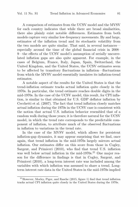
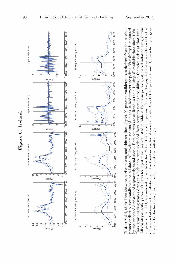
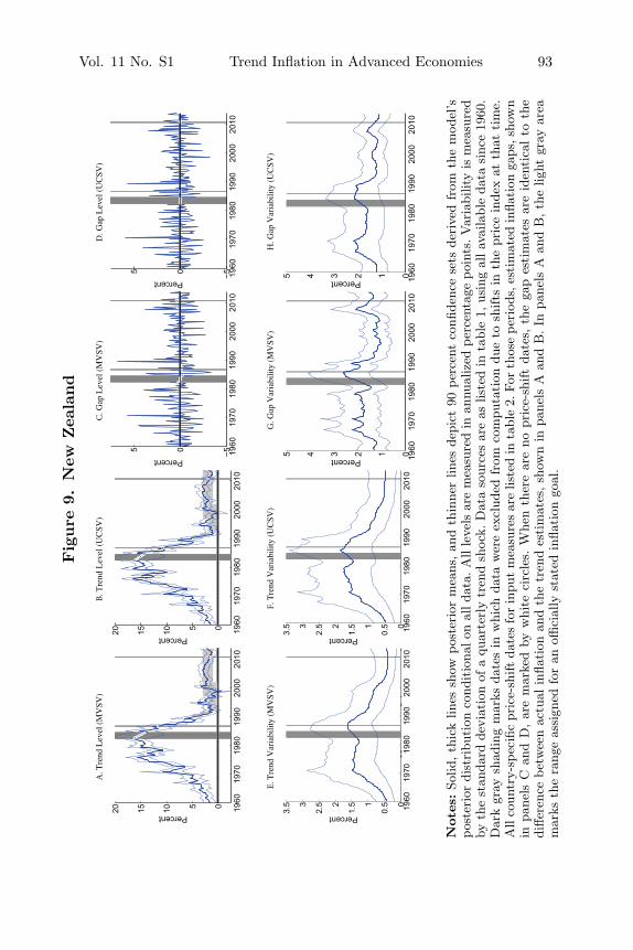
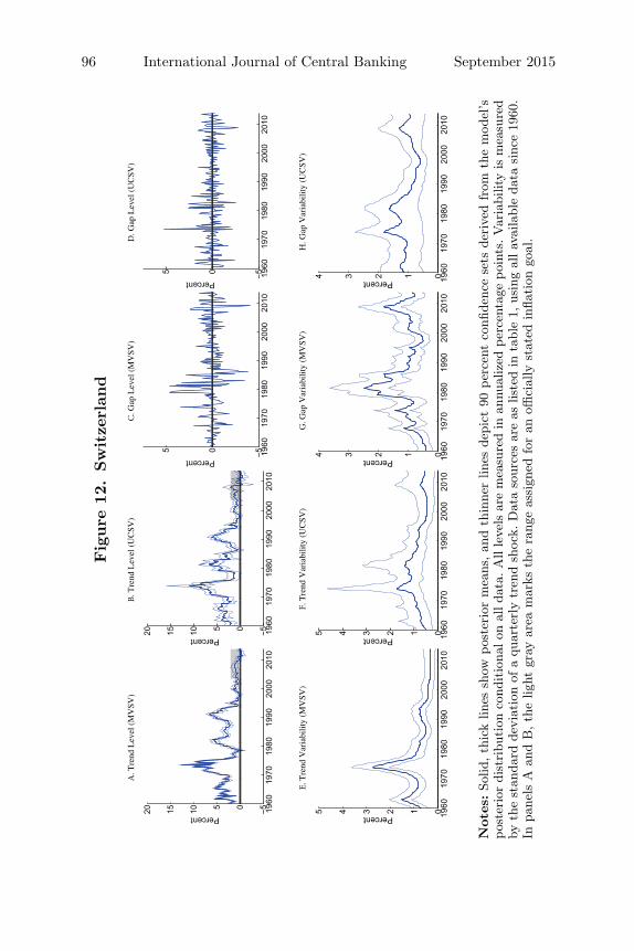
This section reports country-by-country estimates of inflation trendsand gaps as well as their evolving variability, as generated from ourapplication of the UCSV model of Stock and Watson (2007) and ourMVSV model. In essence, these UCSV estimates complement andextend the results reported by Cecchetti et al. (2007), whose esti-mates are conditioned on the GDP deflator inflation rates for theG7 economies. The UCSV estimates reported below are conditionedon the CPI inflation headline rate. We report the inflation-gap esti-mates only for CPI (headline) inflation for the MVSV model, takingthis measure of inflation as the one of greatest interest, particularlyin the context of the targeting and forecasting of inflation. Gen-erally speaking, the estimates reported below are conditioned onall available data from 1960:Q1 through 2013:Q4, the only majorqualification being that we remove from estimation certain dates,specified in table 2, when price shifts occurred.20
19After the introduction of an inflation goal, trend changes are treated as deter-ministic by the MVSV-T model. No country in our data set has abandoned itsinflation goals after inception, except for changes in the goal’s value.
20The effects of these price shifts on our estimates are discussed in section 5.
Vol. 11 No. S1 Trend Inflation in Advanced Economies 81
A comparison of estimates from the UCSV model and the MVSVfor each country indicates that while there are broad similarities,there also plainly exist notable differences. Estimates from bothmodels capture very similar low-frequency movements. By and large,estimates of the inflation trend and its stochastic volatility fromthe two models are quite similar. That said, in several instances—especially around the time of the global financial crisis in 2008–9—the effects of the UCSV model’s assumption of serially uncorre-lated inflation gaps are also quite apparent. For example, in thecases of Belgium, France, Italy, Japan, Spain, Switzerland, theUnited Kingdom, and the United States, the UCSV estimates seemto be affected by transitory fluctuations in inflation—fluctuationsfrom which the MVSV model essentially insulates its inflation-trendestimates.
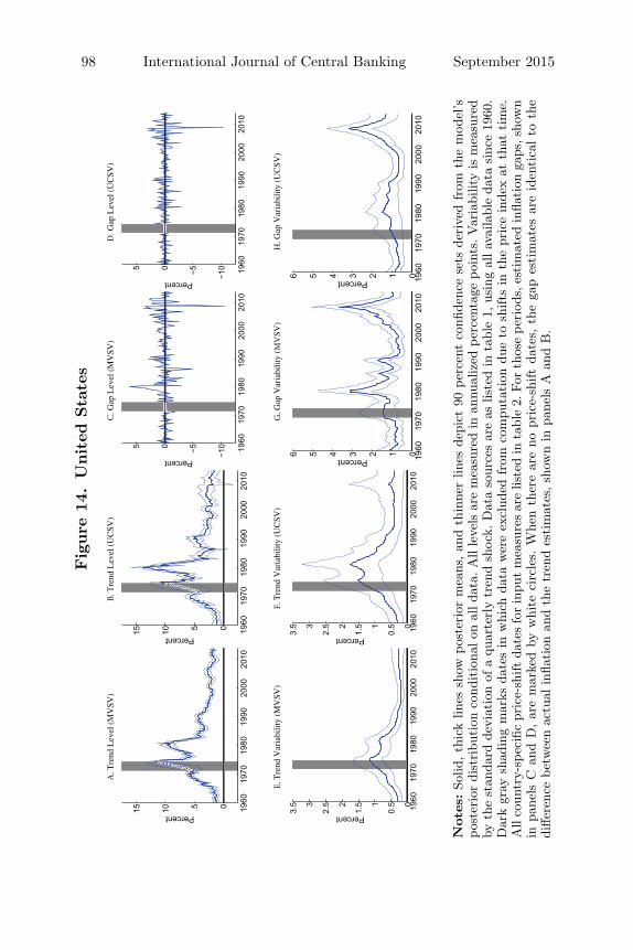
A notable aspect of the results for the United States is that thetrend-inflation estimate tracks actual inflation quite closely in the1970s. In particular, the trend estimate reaches double digits in themid-1970s. In the case of the UCSV model, this result, for CPI infla-tion, is similar to that obtained for U.S. GDP deflator inflation byCecchetti et al. (2007). The fact that trend inflation closely matchesactual inflation during the 1970s in the UCSV case is consistent withthe notion that actual U.S. inflation behavior resembled that of arandom walk during those years; it is therefore natural for the UCSVmodel, in which the trend rate corresponds to the predictable com-ponent of inflation, to attribute much of the observed fluctuationsin inflation to variations in the trend rate.
In the case of the MVSV model, which allows for persistentinflation-gap dynamics, it may appear surprising that we find, onceagain, that trend inflation in the mid-1970s largely mirrors actualinflation. Our estimates differ on this score from those in Cogley,Sargent, and Primiceri (2010), who find that trend U.S. inflationwas well below actual inflation in the mid-1970s.21 One major rea-son for the difference in findings is that in Cogley, Sargent, andPrimiceri (2010), a long-term interest rate was included among thevariables with which inflation was assumed to share a trend. Long-term interest rate data in the United States in the mid-1970s implied
21However, Morley, Piger, and Rasche (2015, figure 1) find that trend inflationtracks actual CPI inflation quite closely in the United States during the 1970s.

82 International Journal of Central Banking September 2015
longer-term inflation expectations far below actual inflation in themid-1970s, and so inclusion of these interest rates in the analysiswould point toward a conclusion that the surge in inflation duringthat period largely amounted to an increase in the inflation gap.22
In our analysis, however, the variables with which we assume CPIinflation has a common trend do not include long-term interest ratesbut do include the GDP deflator inflation rate. In the mid-1970s, theGDP deflator inflation rate exhibited a rise that largely conformedto that of the CPI inflation rate, and so our assumption that thesetwo inflation series have a common trend makes the MVSV modelmore likely to regard the mid-1970s rise in inflation as a rise inthe inflation trend. In contrast, the late-1970s upsurge in inflationwas much steeper for CPI inflation than for the GDP deflator rate.Consequently, our MVSV estimates imply a sharp rise in the CPIinflation gap for this period, as opposed to a surge in trend inflation:see figure 14.
As noted earlier, a great number of countries have introducedformal inflation goals during the sample period. In the majorityof cases, estimated trend levels from both models tend to hoveraround the numerical value for the inflation goal. But there aresome notable exceptions, as discussed below. In the wake of theformal introduction of an inflation target, the stochastic volatil-ity of trend shocks—our measure, alongside the inflation-trendestimate itself, of the degree to which inflation expectations areanchored—decreases in many cases only after some time, about fiveto ten years. This result likely reflects the fact that our measureis conditioned solely on the realized inflation experience of a givencountry.
Among those cases in which countries have explicit inflationgoals, the trend estimates for Sweden, shown in panels A and Bof figure 11, stand out, as the trend has regularly moved below theRiksbank’s inflation target of 2 percent by half a percentage pointor more since the target was introduced in 1993—a finding that
22Likewise, in Mertens’s (2011) estimates of trend inflation for the UnitedStates, both longer-term interest rates and inflation expectations survey dataare assumed to have a common trend with inflation. As both expectations dataand longer-term interest rates registered a much milder rise in the mid-1970s thanactual inflation, their inclusion in the analysis held down the estimated peak oftrend inflation in Mertens (2011).

Vol. 11 No. S1 Trend Inflation in Advanced Economies 83
is consistent with Svensson’s (2015) characterization of the behav-ior of inflation expectations in Sweden. In the same vein, late inthe sample the inflation-trend estimates for Germany and France,joined by Ireland, Italy, and Spain, exhibit inflation-trend estimatessomewhat below the European Central Bank’s target rate of “closeto but below 2 percent.”
A noteworthy comparison between the MVSV and UCSV esti-mates is offered by the case of the United Kingdom, estimates forwhich are displayed in figure 13. For several years late in the sam-ple period, U.K. inflation often persistently exceeded the Bank ofEngland’s 2 percent target, and these overshoots influence our esti-mates in varying degrees. In particular, the UCSV estimates of trendinflation tend to increase in the final years of the sample, with theestimate moving up to levels near 4 percent, and the 90 percent rangefor the estimate of trend inflation barely includes the target rate of2 percent. In contrast, the MVSV model implies a much more lim-ited increase in trend inflation for the United Kingdom, because thepersistence embedded in the model’s specification of inflation-gapdynamics separates the phenomenon of sustained overshoots of theinflation target from the phenomenon of a shift up in trend inflation.
The estimated trend levels of inflation for Japan (shown infigure 8) are, for the latter part of the sample, among the low-est for the countries we study. Both the MVSV and UCSV esti-mates put trend inflation for Japan at levels generally below zerofor the last decade; in particular, the trend estimate derived fromthe MVSV model has been below zero, and even the upper boundof the 90 percent credible set for the trend barely covers valuesabove zero from about 2000 through 2011. Concerns about ele-vated risks of deflation are also raised by our trend estimates forSwitzerland, shown in figure 12, which have steadily been falling,and even moved briefly below zero, over the last few years, afterhaving remained stable near 2 percent for most of the prior fifteenyears.
For most countries, very similar trend estimates are also obtainedif the MVSV model is replaced by a variant that allows for corre-lation between shocks to inflation trend and gaps, in the mannerdescribed in section 3. However, for some countries, this alternativespecification generated noticeably different trend estimates. This hasbeen the case for Germany, Sweden, and Switzerland, results for

84 International Journal of Central Banking September 2015
which are depicted in figure 15. For each of these three countries,the assumption of correlation in the shocks to trend and gaps gen-erates trend estimates that are somewhat less volatile than in thebaseline case—at least when judged by the paths for the pointwiseposterior means. At the same time, uncertainty around these esti-mates, as measured by the width of the 90 percent confidence sets,is considerably wider than in the baseline case, as can be seen fromcomparison of figure 15 with the top-left panels in figures 5, 11,and 12.
For each country, we also derived trend estimates from a fur-ther variant of the MVSV model, one featuring time variation inthe VAR parameters that govern the evolution of the inflation gaps.The results for this variant are very similar to the baseline estimatesshown in figures 1–14. For brevity, the estimates for this variant arenot shown here. The MVSV model with time-varying VAR coef-ficients does, however, generate sizable variation in the estimateddegree of gap persistence, a result brought out in figure 16. Foreach country, gap persistence is measured by the largest absoluteeigenvalue of the gap VAR’s companion form. There is no uniformpattern in the changes of gap persistence implied by these estimates.For some countries, like Canada, New Zealand, and Japan, gap per-sistence seems to have decreased over the latter part of our sam-ple. For other countries, such as France, Ireland, Italy, Sweden, andSwitzerland, gap persistence has rather increased.
Trend estimates from the MVSV-T model are very similar toour baseline estimates, except for the periods when the official infla-tion goal was different from the baseline trend estimates as shownin figures 1–14 (and not shown separately). The MVSV-T modelwill be discussed further in section 7 in the context of forecastevaluation.
5. The Effects of Price-Shift Dates on Trend Estimates
In general, the estimates presented in the previous section arederived from data sets that excluded the observations associatedwith dates at which major price-level shifts occurred due to non-market factors. The results shown in figures 1 to 14 were generatedfrom inflation data for which periods of price shifts are treated as

Vol. 11 No. S1 Trend Inflation in Advanced Economies 85Fig
ure
1.A
ust
ralia
Not
es:So
lid,th
ick
lines
show
post
erio
rm
eans
,an
dth
inne
rlin
esde
pict
90pe
rcen
tco
nfide
nce
sets
deri
ved
from
the
mod
el’s
post
erio
rdi
stri
buti
onco
ndit
iona
lon
alld
ata.
All
leve
lsar
em
easu
red
inan
nual
ized
perc
enta
gepo
ints
.Var
iabi
lity
ism
easu
red
byth
est
anda
rdde
viat
ion
ofa
quar
terl
ytr
end
shoc
k.D
ata
sour
ces
are
aslis
ted
inta
ble
1,us
ing
alla
vaila
ble
data
sinc
e19
60.
Dar
kgr
aysh
adin
gm
arks
date
sin
whi
chda
taw
ere
excl
uded
from
com
puta
tion
due
tosh
ifts
inth
epr
ice
inde
xat
that
tim
e.A
llco
untr
y-sp
ecifi
cpr
ice-
shift
date
sfo
rin
putm
easu
res
are
liste
din
tabl
e2.
Forth
ose
peri
ods,
esti
mat
edin
flati
onga
ps,s
how
nin
pane
lsC
and
D,ar
em
arke
dby
whi
teci
rcle
s.W
hen
ther
ear
eno
pric
e-sh
iftda
tes,
the
gap
esti
mat
esar
eid
enti
calto
the
diffe
renc
ebe
twee
nac
tual
infla
tion
and
the
tren
des
tim
ates
,sh
own
inpa
nels
Aan
dB
.In
pane
lsA
and
B,th
elig
htgr
ayar
eam
arks
the
rang
eas
sign
edfo
ran
offici
ally
stat
edin
flati
ongo
al.

86 International Journal of Central Banking September 2015
Fig
ure
2.B
elgi
um
Not
es:So
lid,th
ick
lines
show
post
erio
rm
eans
,an
dth
inne
rlin
esde
pict
90pe
rcen
tco
nfide
nce
sets
deri
ved
from
the
mod
el’s
post
erio
rdi
stri
buti
onco
ndit
iona
lon
alld
ata.
All
leve
lsar
em
easu
red
inan
nual
ized
perc
enta
gepo
ints
.Var
iabi
lity
ism
easu
red
byth
est
anda
rdde
viat
ion
ofa
quar
terl
ytr
end
shoc
k.D
ata
sour
ces
are
aslis
ted
inta
ble
1,us
ing
alla
vaila
ble
data
sinc
e19
60.
Inpa
nels
Aan
dB
,th
eso
lid,lig
htgr
aylin
em
arks
the
leve
las
sign
edfo
ran
offici
ally
stat
edin
flati
ongo
al.

Vol. 11 No. S1 Trend Inflation in Advanced Economies 87Fig
ure
3.C
anad
a
Not
es:So
lid,th
ick
lines
show
post
erio
rm
eans
,an
dth
inne
rlin
esde
pict
90pe
rcen
tco
nfide
nce
sets
deri
ved
from
the
mod
el’s
post
erio
rdi
stri
buti
onco
ndit
iona
lon
alld
ata.
All
leve
lsar
em
easu
red
inan
nual
ized
perc
enta
gepo
ints
.Var
iabi
lity
ism
easu
red
byth
est
anda
rdde
viat
ion
ofa
quar
terl
ytr
end
shoc
k.D
ata
sour
ces
are
aslis
ted
inta
ble
1,us
ing
alla
vaila
ble
data
sinc
e19
60.
Dar
kgr
aysh
adin
gm
arks
date
sin
whi
chda
taw
ere
excl
uded
from
com
puta
tion
due
tosh
ifts
inth
epr
ice
inde
xat
that
tim
e.A
llco
untr
y-sp
ecifi
cpr
ice-
shift
date
sfo
rin
putm
easu
res
are
liste
din
tabl
e2.
Forth
ose
peri
ods,
esti
mat
edin
flati
onga
ps,s
how
nin
pane
lsC
and
D,ar
em
arke
dby
whi
teci
rcle
s.W
hen
ther
ear
eno
pric
e-sh
iftda
tes,
the
gap
esti
mat
esar
eid
enti
calto
the
diffe
renc
ebe
twee
nac
tual
infla
tion
and
the
tren
des
tim
ates
,sho
wn
inpa
nels
Aan
dB
.In
pane
lsA
and
B,t
heso
lid,l
ight
gray
line
mar
ksth
ele
velas
sign
edfo
ran
offici
ally
stat
edin
flati
ongo
al.

88 International Journal of Central Banking September 2015Fig
ure
4.Fra
nce
Not
es:So
lid,th
ick
lines
show
post
erio
rm
eans
,an
dth
inne
rlin
esde
pict
90pe
rcen
tco
nfide
nce
sets
deri
ved
from
the
mod
el’s
post
erio
rdi
stri
buti
onco
ndit
iona
lon
alld
ata.
All
leve
lsar
em
easu
red
inan
nual
ized
perc
enta
gepo
ints
.Var
iabi
lity
ism
easu
red
byth
est
anda
rdde
viat
ion
ofa
quar
terl
ytr
end
shoc
k.D
ata
sour
ces
are
aslis
ted
inta
ble
1,us
ing
alla
vaila
ble
data
sinc
e19
60.
Dar
kgr
aysh
adin
gm
arks
date
sin
whi
chda
taw
ere
excl
uded
from
com
puta
tion
due
tosh
ifts
inth
epr
ice
inde
xat
that
tim
e.A
llco
untr
y-sp
ecifi
cpr
ice-
shift
date
sfo
rin
putm
easu
res
are
liste
din
tabl
e2.
Forth
ose
peri
ods,
esti
mat
edin
flati
onga
ps,s
how
nin
pane
lsC
and
D,ar
em
arke
dby
whi
teci
rcle
s.W
hen
ther
ear
eno
pric
e-sh
iftda
tes,
the
gap
esti
mat
esar
eid
enti
calto
the
diffe
renc
ebe
twee
nac
tual
infla
tion
and
the
tren
des
tim
ates
,sho
wn
inpa
nels
Aan
dB
.In
pane
lsA
and
B,t
heso
lid,l
ight
gray
line
mar
ksth
ele
velas
sign
edfo
ran
offici
ally
stat
edin
flati
ongo
al.

Vol. 11 No. S1 Trend Inflation in Advanced Economies 89Fig
ure
5.G
erm
any
Not
es:So
lid,th
ick
lines
show
post
erio
rm
eans
,an
dth
inne
rlin
esde
pict
90pe
rcen
tco
nfide
nce
sets
deri
ved
from
the
mod
el’s
post
erio
rdi
stri
buti
onco
ndit
iona
lon
alld
ata.
All
leve
lsar
em
easu
red
inan
nual
ized
perc
enta
gepo
ints
.Var
iabi
lity
ism
easu
red
byth
est
anda
rdde
viat
ion
ofa
quar
terl
ytr
end
shoc
k.D
ata
sour
ces
are
aslis
ted
inta
ble
1,us
ing
alla
vaila
ble
data
sinc
e19
60.
Dar
kgr
aysh
adin
gm
arks
date
sin
whi
chda
taw
ere
excl
uded
from
com
puta
tion
due
tosh
ifts
inth
epr
ice
inde
xat
that
tim
e.A
llco
untr
y-sp
ecifi
cpr
ice-
shift
date
sfo
rin
putm
easu
res
are
liste
din
tabl
e2.
Forth
ose
peri
ods,
esti
mat
edin
flati
onga
ps,s
how
nin
pane
lsC
and
D,ar
em
arke
dby
whi
teci
rcle
s.W
hen
ther
ear
eno
pric
e-sh
iftda
tes,
the
gap
esti
mat
esar
eid
enti
calto
the
diffe
renc
ebe
twee
nac
tual
infla
tion
and
the
tren
des
tim
ates
,sho
wn
inpa
nels
Aan
dB
.In
pane
lsA
and
B,t
heso
lid,l
ight
gray
line
mar
ksth
ele
velas
sign
edfo
ran
offici
ally
stat
edin
flati
ongo
al.
90 International Journal of Central Banking September 2015Fig
ure
6.Ir
elan
d
Not
es:So
lid,th
ick
lines
show
post
erio
rm
eans
,an
dth
inne
rlin
esde
pict
90pe
rcen
tco
nfide
nce
sets
deri
ved
from
the
mod
el’s
post
erio
rdi
stri
buti
onco
ndit
iona
lon
alld
ata.
All
leve
lsar
em
easu
red
inan
nual
ized
perc
enta
gepo
ints
.Var
iabi
lity
ism
easu
red
byth
est
anda
rdde
viat
ion
ofa
quar
terl
ytr
end
shoc
k.D
ata
sour
ces
are
aslis
ted
inta
ble
1,us
ing
alla
vaila
ble
data
sinc
e19
60.
Dar
kgr
aysh
adin
gm
arks
date
sin
whi
chda
taw
ere
excl
uded
from
com
puta
tion
due
tosh
ifts
inth
epr
ice
inde
xat
that
tim
e.A
llco
untr
y-sp
ecifi
cpr
ice-
shift
date
sfo
rin
putm
easu
res
are
liste
din
tabl
e2.
Forth
ose
peri
ods,
esti
mat
edin
flati
onga
ps,s
how
nin
pane
lsC
and
D,ar
em
arke
dby
whi
teci
rcle
s.W
hen
ther
ear
eno
pric
e-sh
iftda
tes,
the
gap
esti
mat
esar
eid
enti
calto
the
diffe
renc
ebe
twee
nac
tual
infla
tion
and
the
tren
des
tim
ates
,sho
wn
inpa
nels
Aan
dB
.In
pane
lsA
and
B,t
heso
lid,l
ight
gray
line
mar
ksth
ele
velas
sign
edfo
ran
offici
ally
stat
edin
flati
ongo
al.

Vol. 11 No. S1 Trend Inflation in Advanced Economies 91
Fig
ure
7.It
aly
Not
es:So
lid,th
ick
lines
show
post
erio
rm
eans
,an
dth
inne
rlin
esde
pict
90pe
rcen
tco
nfide
nce
sets
deri
ved
from
the
mod
el’s
post
erio
rdi
stri
buti
onco
ndit
iona
lon
alld
ata.
All
leve
lsar
em
easu
red
inan
nual
ized
perc
enta
gepo
ints
.Var
iabi
lity
ism
easu
red
byth
est
anda
rdde
viat
ion
ofa
quar
terl
ytr
end
shoc
k.D
ata
sour
ces
are
aslis
ted
inta
ble
1,us
ing
alla
vaila
ble
data
sinc
e19
60.
Inpa
nels
Aan
dB
,th
eso
lid,lig
htgr
aylin
em
arks
the
leve
las
sign
edfo
ran
offici
ally
stat
edin
flati
ongo
al.

92 International Journal of Central Banking September 2015Fig
ure
8.Ja
pan
Not
es:So
lid,th
ick
lines
show
post
erio
rm
eans
,an
dth
inne
rlin
esde
pict
90pe
rcen
tco
nfide
nce
sets
deri
ved
from
the
mod
el’s
post
erio
rdi
stri
buti
onco
ndit
iona
lon
alld
ata.
All
leve
lsar
em
easu
red
inan
nual
ized
perc
enta
gepo
ints
.Var
iabi
lity
ism
easu
red
byth
est
anda
rdde
viat
ion
ofa
quar
terl
ytr
end
shoc
k.D
ata
sour
ces
are
aslis
ted
inta
ble
1,us
ing
alla
vaila
ble
data
sinc
e19
60.
Dar
kgr
aysh
adin
gm
arks
date
sin
whi
chda
taw
ere
excl
uded
from
com
puta
tion
due
tosh
ifts
inth
epr
ice
inde
xat
that
tim
e.A
llco
untr
y-sp
ecifi
cpr
ice-
shift
date
sfo
rin
putm
easu
res
are
liste
din
tabl
e2.
Forth
ose
peri
ods,
esti
mat
edin
flati
onga
ps,s
how
nin
pane
lsC
and
D,ar
em
arke
dby
whi
teci
rcle
s.W
hen
ther
ear
eno
pric
e-sh
iftda
tes,
the
gap
esti
mat
esar
eid
enti
calto
the
diffe
renc
ebe
twee
nac
tual
infla
tion
and
the
tren
des
tim
ates
,sh
own
inpa
nels
Aan
dB
.
Vol. 11 No. S1 Trend Inflation in Advanced Economies 93Fig
ure
9.N
ewZea
land
Not
es:So
lid,th
ick
lines
show
post
erio
rm
eans
,an
dth
inne
rlin
esde
pict
90pe
rcen
tco
nfide
nce
sets
deri
ved
from
the
mod
el’s
post
erio
rdi
stri
buti
onco
ndit
iona
lon
alld
ata.
All
leve
lsar
em
easu
red
inan
nual
ized
perc
enta
gepo
ints
.Var
iabi
lity
ism
easu
red
byth
est
anda
rdde
viat
ion
ofa
quar
terl
ytr
end
shoc
k.D
ata
sour
ces
are
aslis
ted
inta
ble
1,us
ing
alla
vaila
ble
data
sinc
e19
60.
Dar
kgr
aysh
adin
gm
arks
date
sin
whi
chda
taw
ere
excl
uded
from
com
puta
tion
due
tosh
ifts
inth
epr
ice
inde
xat
that
tim
e.A
llco
untr
y-sp
ecifi
cpr
ice-
shift
date
sfo
rin
putm
easu
res
are
liste
din
tabl
e2.
Forth
ose
peri
ods,
esti
mat
edin
flati
onga
ps,s
how
nin
pane
lsC
and
D,ar
em
arke
dby
whi
teci
rcle
s.W
hen
ther
ear
eno
pric
e-sh
iftda
tes,
the
gap
esti
mat
esar
eid
enti
calto
the
diffe
renc
ebe
twee
nac
tual
infla
tion
and
the
tren
des
tim
ates
,sh
own
inpa
nels
Aan
dB
.In
pane
lsA
and
B,th
elig
htgr
ayar
eam
arks
the
rang
eas
sign
edfo
ran
offici
ally
stat
edin
flati
ongo
al.

94 International Journal of Central Banking September 2015Fig
ure
10.
Spai
n
Not
es:So
lid,th
ick
lines
show
post
erio
rm
eans
,an
dth
inne
rlin
esde
pict
90pe
rcen
tco
nfide
nce
sets
deri
ved
from
the
mod
el’s
post
erio
rdi
stri
buti
onco
ndit
iona
lon
alld
ata.
All
leve
lsar
em
easu
red
inan
nual
ized
perc
enta
gepo
ints
.Var
iabi
lity
ism
easu
red
byth
est
anda
rdde
viat
ion
ofa
quar
terl
ytr
end
shoc
k.D
ata
sour
ces
are
aslis
ted
inta
ble
1,us
ing
alla
vaila
ble
data
sinc
e19
60.
Dar
kgr
aysh
adin
gm
arks
date
sin
whi
chda
taw
ere
excl
uded
from
com
puta
tion
due
tosh
ifts
inth
epr
ice
inde
xat
that
tim
e.A
llco
untr
y-sp
ecifi
cpr
ice-
shift
date
sfo
rin
putm
easu
res
are
liste
din
tabl
e2.
Forth
ose
peri
ods,
esti
mat
edin
flati
onga
ps,s
how
nin
pane
lsC
and
D,ar
em
arke
dby
whi
teci
rcle
s.W
hen
ther
ear
eno
pric
e-sh
iftda
tes,
the
gap
esti
mat
esar
eid
enti
calto
the
diffe
renc
ebe
twee
nac
tual
infla
tion
and
the
tren
des
tim
ates
,sho
wn
inpa
nels
Aan
dB
.In
pane
lsA
and
B,t
heso
lid,l
ight
gray
line
mar
ksth
ele
velas
sign
edfo
ran
offici
ally
stat
edin
flati
ongo
al.

Vol. 11 No. S1 Trend Inflation in Advanced Economies 95Fig
ure
11.
Sw
eden
Not
es:So
lid,th
ick
lines
show
post
erio
rm
eans
,an
dth
inne
rlin
esde
pict
90pe
rcen
tco
nfide
nce
sets
deri
ved
from
the
mod
el’s
post
erio
rdi
stri
buti
onco
ndit
iona
lon
alld
ata.
All
leve
lsar
em
easu
red
inan
nual
ized
perc
enta
gepo
ints
.Var
iabi
lity
ism
easu
red
byth
est
anda
rdde
viat
ion
ofa
quar
terl
ytr
end
shoc
k.D
ata
sour
ces
are
aslis
ted
inta
ble
1,us
ing
alla
vaila
ble
data
sinc
e19
60.
Dar
kgr
aysh
adin
gm
arks
date
sin
whi
chda
taw
ere
excl
uded
from
com
puta
tion
due
tosh
ifts
inth
epr
ice
inde
xat
that
tim
e.A
llco
untr
y-sp
ecifi
cpr
ice-
shift
date
sfo
rin
putm
easu
res
are
liste
din
tabl
e2.
Forth
ose
peri
ods,
esti
mat
edin
flati
onga
ps,s
how
nin
pane
lsC
and
D,ar
em
arke
dby
whi
teci
rcle
s.W
hen
ther
ear
eno
pric
e-sh
iftda
tes,
the
gap
esti
mat
esar
eid
enti
calto
the
diffe
renc
ebe
twee
nac
tual
infla
tion
and
the
tren
des
tim
ates
,sho
wn
inpa
nels
Aan
dB
.In
pane
lsA
and
B,t
heso
lid,l
ight
gray
line
mar
ksth
ele
velas
sign
edfo
ran
offici
ally
stat
edin
flati
ongo
al.
96 International Journal of Central Banking September 2015
Fig
ure
12.
Sw
itze
rlan
d
Not
es:So
lid,th
ick
lines
show
post
erio
rm
eans
,an
dth
inne
rlin
esde
pict
90pe
rcen
tco
nfide
nce
sets
deri
ved
from
the
mod
el’s
post
erio
rdi
stri
buti
onco
ndit
iona
lon
alld
ata.
All
leve
lsar
em
easu
red
inan
nual
ized
perc
enta
gepo
ints
.Var
iabi
lity
ism
easu
red
byth
est
anda
rdde
viat
ion
ofa
quar
terl
ytr
end
shoc
k.D
ata
sour
ces
are
aslis
ted
inta
ble
1,us
ing
alla
vaila
ble
data
sinc
e19
60.
Inpa
nels
Aan
dB
,th
elig
htgr
ayar
eam
arks
the
rang
eas
sign
edfo
ran
offici
ally
stat
edin
flati
ongo
al.

Vol. 11 No. S1 Trend Inflation in Advanced Economies 97Fig
ure
13.
United
Kin
gdom
Not
es:So
lid,th
ick
lines
show
post
erio
rm
eans
,an
dth
inne
rlin
esde
pict
90pe
rcen
tco
nfide
nce
sets
deri
ved
from
the
mod
el’s
post
erio
rdi
stri
buti
onco
ndit
iona
lon
alld
ata.
All
leve
lsar
em
easu
red
inan
nual
ized
perc
enta
gepo
ints
.Var
iabi
lity
ism
easu
red
byth
est
anda
rdde
viat
ion
ofa
quar
terl
ytr
end
shoc
k.D
ata
sour
ces
are
aslis
ted
inta
ble
1,us
ing
alla
vaila
ble
data
sinc
e19
60.
Dar
kgr
aysh
adin
gm
arks
date
sin
whi
chda
taw
ere
excl
uded
from
com
puta
tion
due
tosh
ifts
inth
epr
ice
inde
xat
that
tim
e.A
llco
untr
y-sp
ecifi
cpr
ice-
shift
date
sfo
rin
putm
easu
res
are
liste
din
tabl
e2.
Forth
ose
peri
ods,
esti
mat
edin
flati
onga
ps,s
how
nin
pane
lsC
and
D,ar
em
arke
dby
whi
teci
rcle
s.W
hen
ther
ear
eno
pric
e-sh
iftda
tes,
the
gap
esti
mat
esar
eid
enti
calto
the
diffe
renc
ebe
twee
nac
tual
infla
tion
and
the
tren
des
tim
ates
,sho
wn
inpa
nels
Aan
dB
.In
pane
lsA
and
B,t
heso
lid,l
ight
gray
line
mar
ksth
ele
velas
sign
edfo
ran
offici
ally
stat
edin
flati
ongo
al.
98 International Journal of Central Banking September 2015Fig
ure
14.
United
Sta
tes
Not
es:So
lid,th
ick
lines
show
post
erio
rm
eans
,an
dth
inne
rlin
esde
pict
90pe
rcen
tco
nfide
nce
sets
deri
ved
from
the
mod
el’s
post
erio
rdi
stri
buti
onco
ndit
iona
lon
alld
ata.
All
leve
lsar
em
easu
red
inan
nual
ized
perc
enta
gepo
ints
.Var
iabi
lity
ism
easu
red
byth
est
anda
rdde
viat
ion
ofa
quar
terl
ytr
end
shoc
k.D
ata
sour
ces
are
aslis
ted
inta
ble
1,us
ing
alla
vaila
ble
data
sinc
e19
60.
Dar
kgr
aysh
adin
gm
arks
date
sin
whi
chda
taw
ere
excl
uded
from
com
puta
tion
due
tosh
ifts
inth
epr
ice
inde
xat
that
tim
e.A
llco
untr
y-sp
ecifi
cpr
ice-
shift
date
sfo
rin
putm
easu
res
are
liste
din
tabl
e2.
Forth
ose
peri
ods,
esti
mat
edin
flati
onga
ps,s
how
nin
pane
lsC
and
D,ar
em
arke
dby
whi
teci
rcle
s.W
hen
ther
ear
eno
pric
e-sh
iftda
tes,
the
gap
esti
mat
esar
eid
enti
calto
the
diffe
renc
ebe
twee
nac
tual
infla
tion
and
the
tren
des
tim
ates
,sh
own
inpa
nels
Aan
dB
.

Vol. 11 No. S1 Trend Inflation in Advanced Economies 99
Figure 15. Trend Estimates with Correlation betweenShocks to Trend and Gaps
Notes: In each panel, solid lines depict estimates derived from a version of theMVSV model that allows for correlation between the shocks to trend and gapinflation. Dashed lines show the corresponding estimates from a baseline speci-ficton where shocks to trend and gaps are assumed to be uncorrelated. Esti-mates are obtained from data that treat the price-shift dates listed in table 2 asmissing observations. Solid, thick lines show posterior means, and thinner linesdepict 90 percent confidence sets derived from the model’s posterior distribu-tion conditional on all data. All series are measured in annualized percentagepoints (as approximated by log-changes).

100 International Journal of Central Banking September 2015
Fig
ure
16.
Gap
Per
sist
ence
(con
tinu
ed)

Vol. 11 No. S1 Trend Inflation in Advanced Economies 101Fig
ure
16.
(Con
tinued
)
Not
es:
Thi
ckso
lidlin
esde
pict
post
erio
rm
eans
ofth
ela
rges
t,ab
solu
teei
genv
alue
ofth
eco
mpa
nion
mat
rix
asso
ciat
edw
ith
the
VA
Rfo
rga
pin
flati
onin
ave
rsio
nof
the
MV
SVm
odel
wit
hti
me-
vary
ing
VA
Rpa
ram
eter
s;th
inlin
esde
pict
the
inte
rqua
r-ti
lera
nge.
Cor
resp
ondi
nges
tim
ates
obta
ined
from
our
base
line
spec
ifica
tion
wit
hco
nsta
ntVA
Rpa
ram
eter
sar
ede
pict
edby
dash
edlin
es.E
stim
ates
are
obta
ined
from
data
that
trea
tth
epr
ice-
shift
date
slis
ted
inta
ble
2as
mis
sing
obse
rvat
ions
.

102 International Journal of Central Banking September 2015
missing values in each model’s estimation.23 The relevance of theseepisodes for our estimates, as brought out by a comparison withestimates conditional on all data, is the subject of this section.
In all, we consider fifteen price-shift episodes affecting seven outof the fourteen countries in our sample; all are listed in table 2.Most episodes are related to increases in taxes on goods and ser-vices and similar administrative imposts; in these instances, only asingle quarterly observation is omitted from the data. The rationalefor excluding inflation observations for these specified dates is thatthe price level shifted in the period in question not as a reflection ofmonetary policy or of private-sector-initiated behavior, but becauseof a non-monetary governmental measure whose effect was essen-tially to rescale the price level. Only four episodes stretched beyonda year or more: the periods of official price controls in the UnitedStates (1971–4), the United Kingdom (1972–4), and New Zealand(1982–4), as well as the transition period in the wake of Germanreunification (1991).24 Again, the shift in the price level in thesedates corresponded either to a movement away from market deter-mination of prices (in the case of the price-control periods) or amajor redefinition of the area covered by the price index (as whenthe former East Germany was brought into the Federal Republic ofGermany).25
23In the case of price controls, this procedure amounts to interpolating betweenthe final value of inflation recorded before the imposition of price controls and thefirst observation on inflation occurring after the period in which controls werelifted. An alternative interpolation procedure would have involved constraininginflation during the omitted quarters to be equal to the average value of inflationobserved over those quarters. This alternative procedure would have capturedthe idea that, when price controls are lifted, the price level catches up to thevalue it would have reached in the absence of controls. However, following thisalternative procedure would have meant treating price controls in a different wayfrom other price shifts that we consider, such as changes in indirect taxes.
24We treat the whole of 1991 as a price shift for Germany, following Levin andPiger (2004).
25Gordon (1983) and Staiger, Stock, and Watson (1997) figure among previ-ous studies that allow for the effects of price controls in their study of inflationdynamics, while Levin and Piger’s (2004) study of international inflation dynam-ics allows for major changes in national sales taxes. In addition, the exclusion ofcontrol and tax periods from the estimates represents a step in the direction ofincorporating historical information about individual countries’ experiences intothe study of inflation dynamics, as recommended by Cecchetti et al. (2007).

Vol. 11 No. S1 Trend Inflation in Advanced Economies 103
Reflecting their typically short duration, the price-shift dates arenot associated with a great impact on trend estimates for many coun-tries. This is not invariably the case, however. Figure 17 presentstrend estimates for four countries—Germany, Ireland, New Zealand,and the United States—for which the inclusion of price-shift dateshas different effects on trend estimates. The figure presents a com-parison of trend estimates discussed in the previous section withestimates that condition on the entire data, including inflationdata recorded during the price-shift episodes. For each country,the effects of including price-shift dates on trend estimates fromthe MVSV model are qualitatively similar to those on the UCSVestimates.
The price-shift episodes of longer duration evidently can havequite sizable effects on trend estimates. For example, estimatesof trend inflation in the United States—whether derived from theUCSV or the MVSV model—peak well above 10 percent in the mid-1970s, when conditioned on all observations, whereas for the case inwhich the price-shift episode is treated as a period of missing data,the estimated inflation trend rises only gradually from about 5 to justbelow 10 percent. This correction may well, of course, be consideredexcessive, as it leads to much of the mid-1970s rise in inflation beingclassed as transitory. The fact that the rise in inflation in the UnitedStates in the mid-1970s was preceded by a lengthy and substantialmonetary expansion points instead to the possibility that a good dealof the rise in inflation amounted, instead, to an increase in the trendrate of inflation. But even our price-shift-adjusted model estimateslargely attribute the mid-1970s peak of inflation to a rise in trend. Inparticular, and as earlier noted, the MVSV model’s characterizationof the rise in CPI inflation in the mid-1970s as largely comprisingan increase in trend inflation in good part reflects the fact that theincrease in GDP deflator inflation over the same period basicallyconfirmed the picture provided by CPI inflation behavior. For bothof the U.S. inflation-trend estimates (that is, MVSV and UCSV), theeffect of allowing for the 1971–4 price-control episode is not to lowersubstantially the rise in trend inflation, but instead to remove thedecline in trend inflation that is registered in the controls-affectedyear of 1972—when measured inflation exhibited a decline that waslikely spurious.

104 International Journal of Central Banking September 2015Fig
ure
17.
Tre
nd
Est
imat
esan
dP
rice
-Shift
Dat
es
Not
es:In
each
pane
l,th
ick
gray
lines
depi
ctes
tim
ates
cond
itio
ned
onda
tase
ts,w
here
pric
e-sh
iftda
tes
have
been
rem
oved
,w
here
asda
rkso
lidlin
esde
pict
esti
mat
esco
ndit
ione
don
allin
flati
onda
ta.Fo
rea
chco
untr
y,se
para
tepa
nels
disp
lay
resu
lts
from
the
MV
SVm
odel
and
the
UC
SVm
odel
.G
ray
shad
ing
mar
ksda
tes
inw
hich
data
wer
eex
clud
edfr
omco
mpu
tati
ondu
eto
shift
sin
the
pric
ein
dex
atth
atti
me.
All
coun
try-
spec
ific
pric
e-sh
iftda
tesfo
rin
putm
easu
resar
elis
ted
inta
ble
2.T
hin
lines
deno
teth
eac
tual
data
for
the
head
line
CP
Iin
dex.
All
leve
lsar
em
easu
red
inan
nual
ized
perc
enta
gepo
ints
(as
appr
oxim
ated
bylo
g-ch
ange
s).

Vol. 11 No. S1 Trend Inflation in Advanced Economies 105
6. Trend Estimates in Quasi-Real Time
The trend estimates described in the previous two sections have beenconditioned on full-sample data—with or without price shifts. Suchestimates are typically labeled “smoothed” estimates, as distinctfrom “quasi-real-time” estimates, to use the terminology familiarfrom Orphanides and van Norden (2002). These real-time estimates,which we shall also refer to as “filtered” estimates, generate theinflation trend for time t solely on the basis of data observations upto and including time t. We now derive such quasi-real-time esti-mates by reestimating each for each quarter from 1984:Q4 through2013:Q4, using all available data from 1960:Q1 onwards. The dif-ference between quasi-real-time and smoothed estimates reflects theeffects of reestimating the model’s hyperparameters like ϕh, gov-erning the volatility of shocks to the stochastic log-variances, or thecoefficients A(L) of the gap-based VAR. Our analysis abstracts fromdata revisions as a source of difference between real-time estimatesof trend inflation and our inflation data. Rather, the data we usethroughout are from what is essentially a single vintage that wecollected in 2014.26
Ahead of our analysis in section 7 of each model’s forecast perfor-mance based on this quasi-real-time analysis, this section providesa comparison of smoothed and filtered estimates of trend inflationfrom the MVSV model, as well as the difference between filtered esti-mates of trend inflation between the UCSV and the MVSV model.
Two results stand out from this comparison. We discuss each inturn.
First, filtered trend estimates from the MVSV model are fairlyclose to their smoothed counterparts, as can be seen in figure 18.Overall, as is to be expected, the smoothed estimates are a littleless variable than their quasi-real-time counterparts. Smoothed esti-mates are designed to be more precise estimates of the underlyinginflation trend, and they benefit from knowledge regarding the sub-sequent behavior of realized inflation. For this reason, they may not
26An alternative notion of “filtered” estimates, not pursued here, would be onein which the model’s hyperparameters were taken as given—as would be the case,for example, if values estimated based on the full sample of data were used—sothat only the values of the model’s latent states (like the level of trend inflationand the stochastic volatility in trend and gaps) needed to be estimated.

106 International Journal of Central Banking September 2015
Fig
ure
18.
Sm
oot
hed
and
Filte
red
Tre
nd
Est
imat
es(M
VSV
model
)
(con
tinu
ed)
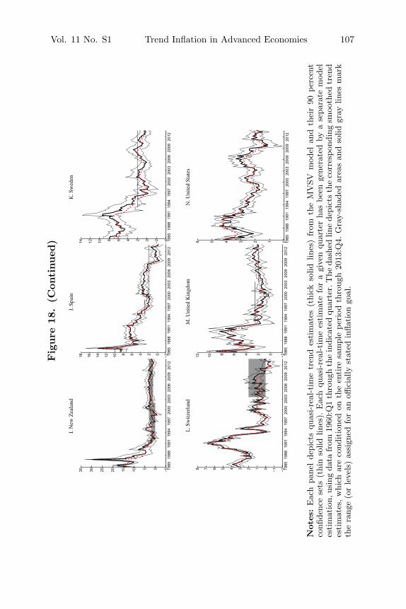
Vol. 11 No. S1 Trend Inflation in Advanced Economies 107Fig
ure
18.
(Con
tinued
)
Not
es:
Eac
hpa
nel
depi
cts
quas
i-re
al-t
ime
tren
des
tim
ates
(thi
ckso
lidlin
es)
from
the
MV
SVm
odel
and
thei
r90
perc
ent
confi
denc
ese
ts(t
hin
solid
lines
).E
ach
quas
i-re
al-t
ime
esti
mat
efo
ra
give
nqu
arte
rha
sbe
enge
nera
ted
bya
sepa
rate
mod
eles
tim
atio
n,us
ing
data
from
1960
:Q1
thro
ugh
the
indi
cate
dqu
arte
r.T
heda
shed
line
depi
ctsth
eco
rres
pond
ing
smoo
thed
tren
des
tim
ates
,w
hich
are
cond
itio
ned
onth
een
tire
sam
ple
peri
odth
roug
h20
13:Q
4.G
ray-
shad
edar
eas
and
solid
gray
lines
mar
kth
era
nge
(or
leve
ls)
assi
gned
for
anoffi
cial
lyst
ated
infla
tion
goal
.

108 International Journal of Central Banking September 2015
lend themselves to exercises such as determining the exact timingof events, such as the point at which an inflation target becamecredible. The filtered estimates might thus be more suitable forcomparison against other measures of trend inflation derived fromfinancial market indicators. But, at least in the case of the multi-variate model, the differences between smoothed and quasi-real-timeestimates appear to be fairly small. For example, as can be seen infigure 18, both estimates provide similar signals regarding the extentto which trend inflation is aligned with different countries’ officialinflation targets.
Second, filtered trend estimates from the UCSV model seem moreprone to overreact to transitory changes in inflation than the MVSVmodel. A similar distinction has been noted previously in the con-text of smoothed estimates for both models. But the differencesare especially striking in the case of the quasi-real-time estimatesshown in figure 19. In particular, for the years 2006–12, considerableswings in commodity prices played a major role in observed fluctua-tions in inflation rates in many countries. And after 2009, persistentsigns of disinflationary pressure are far more manifest in the MVSVmodel’s quasi-real-time estimates of the inflation trend in a numberof economies—notably the euro area, Japan, Sweden, the UnitedKingdom, and the United States—than in the UCSV estimates.
7. Forecast Evaluation
Trend inflation is a latent and unobservable variable. Some prop-erties of the MVSV estimates documented in the previous sectionsmight appear more appealing than their UCSV counterparts, butsuch a conclusion might well rely more on a subjective impression ofwhat constitutes a “reasonable” estimate rather than a direct com-parison between estimated and actual values of trend inflation—acomparison that by its very nature is infeasible. In the absence ofsuch a direct comparison, an indirect way of assessing the valid-ity, or usefulness, of different trend estimates is to evaluate infla-tion forecasts generated by each model at some finite horizons. Theidea behind this approach is that, just as the Beveridge-Nelsontrend is derived from solving a long-run forecasting problem, amodel that allows explicitly for an evolving trend in the inflationrate should generate satisfactory inflation forecasts, and probably

Vol. 11 No. S1 Trend Inflation in Advanced Economies 109
Fig
ure
19.
Com
par
ison
ofFilte
red
Tre
nd
Est
imat
es
(con
tinu
ed)

110 International Journal of Central Banking September 2015
Fig
ure
19.
(Con
tinued
)
Not
es:E
ach
pane
lsho
ws
quas
i-re
al-t
ime
tren
des
tim
ates
from
the
MV
SVm
odel
(sol
id)
and
the
UC
SVm
odel
(das
hed)
.Eac
hqu
asi-re
al-t
ime
esti
mat
efo
ra
give
nqu
arte
rha
sbe
enge
nera
ted
bya
sepa
rate
mod
eles
tim
atio
n,us
ing
data
from
1960
:Q1
thro
ugh
that
quar
ter.
Thi
nso
lidlin
esde
pict
CP
Ihe
adlin
ein
flati
onda
ta.
Gra
y-sh
aded
area
san
dso
lidgr
aylin
esm
ark
the
rang
e(o
rle
vels
)as
sign
edfo
ran
offici
ally
stat
edin
flati
ongo
al.

Vol. 11 No. S1 Trend Inflation in Advanced Economies 111
also at horizons shorter than the very long run. Evaluating theforecast performance of different trend-inflation models may be anenlightening basis on which to assess different trend estimates; itshould also be relevant for researchers who are especially concernedwith generating good inflation forecasts. As argued by Faust andWright (2013), sound procedures for obtaining inflation forecastslikely include grounding those forecasts on an explicit measure ofthe trend-inflation rate.
This section evaluates forecasts of CPI headline inflation up tofour years ahead derived from the UCSV and MVSV model for eachcountry. In addition, we also consider forecasts motivated by therandom-walk benchmark of Atkeson and Ohanian (2001). For thisbenchmark, inflation forecasts for all horizons are taken as equal toa four-quarter or, alternatively, a twelve-quarter moving average oflagged inflation. Inflation forecasts are generated in quasi-real timefrom 1985 onwards. The first forecast is therefore conditioned onmodel estimates obtained for data from 1960:Q1 through 1984:Q4,with an increasing estimation window as the forecast period isshifted forward (that is, as steadily more observations are used in theestimation sample). Every jumping-off date considered is associatedwith reestimation of each model.27
For each quarter considered, we generate inflation forecasts bothfor annual (that is, four-quarter) inflation rates (computed as theaverage of expected inflation rates over four consecutive quarters)and for quarterly changes at different horizons.28 Annual infla-tion rates are forecast for the upcoming four quarters, one yearahead (quarters 5–8), two years ahead (quarters 9–12), three yearsahead (quarters 13–16), and four years ahead (quarters 17–20).Quarterly inflation rates are forecast for the next quarter, thenfour, eight, twelve, and sixteen quarters ahead. Results are notparticularly sensitive to the inclusion of the price-shift dates dis-cussed in section 5—which mostly occurred prior to the 1985–2013period spanned by our various forecast windows—and all results are
27As before, our analysis abstracts from discrepancies between real-time meas-ures of inflation and our inflation data that might have arisen from data revisions.
28Stock and Watson (2009) also focus on forecasts of one-year or two-yearpercentage changes in the price level, whereas Faust and Wright (2013) studyforecasts of quarterly inflation rates.

112 International Journal of Central Banking September 2015
derived from data that include observed inflation for the price-shiftdates.
In our application, we measure forecast accuracy using root meansquared errors (“RMSE”) and average log-predictive scores, whichare reported in table 3 for forecasts of annual inflation and table 4 forquarterly inflation rates. In both cases, inflation rates are expressedin annual percentage units.
Log-predictive scores measure the accuracy of a model’s predic-tive density and are computed here for the UCSV, MVSV, andMVSV-T model.29 As in Adolfson, Linde, and Villani (2007) andClark and Ravazzolo (2014), we approximate the predictive den-sity with a normal distribution and compute mean and variance ofthe predictive density by integrating over the draws generated bythe MCMC sampler.30 Denoting the predictive mean and varianceat time t for inflation πt+h by μt+h|t and σ2
t+h|t, respectively, thelog-predictive score at t is given by
lt+h|t = −0.5
(log(2 · π) + log(σ2
t+h|t) +(πt+h − μt+h|t)2
σ2t+h|t
)
and the average log-predictive score is computed by averaging lt+h|tacross all forecasts t for a given forecast horizon h. Whereas theRMSE reflects only the quality of the mean of the predictive den-sity, the normal approximation of the log-density score has theproperty that it also evaluates the squared errors in relation toforecast uncertainty as measured by the variance of the predictivedensity.
In tables 3 and 4, forecast performance of alternative models ismeasured by the ratio of each model’s RMSE compared with theMVSV model as well as the difference between the average log-predictive scores (where applicable). A value below unity of the
29The moving averages generate only mean predictions without specifying apredictive density.
30Conditional on draws of model parameters and levels and volatilities of theinflation trend and gap, it is straightforward to compute the predictive meansusing standard formulas. Predictive variances can readily be computed by adapt-ing formulas shown in Cogley and Sargent (2015). The laws of iterated expecta-tions and total variances can then be used to compute the predictive mean andvariance over all MCMC draws.

Vol. 11 No. S1 Trend Inflation in Advanced Economies 113
Tab
le3.
For
ecas
tEva
luat
ion:A
nnual
Inflat
ion
Rat
es
Yea
rsA
hea
d
Nex
t1
Yea
r2
Yea
rs3
Yea
rs4
Yea
rs
Aus
tral
iaR
MSE
for
MV
SV1.
742.
282.
562.
772.
71–
Rel
ativ
eto
MA
(4)
0.89
∗0.
920.
93∗
0.95
0.95
–R
elat
ive
toM
A(1
2)0.
860.
981.
041.
070.
99–
Rel
ativ
eto
MV
SV-T
rend
1.00
1.00
1.00
1.00
∗∗1.
00∗∗
–R
elat
ive
toU
CSV
0.90
0.92
0.92
0.94
0.93
–R
elat
ive
toM
VSV
-T1.
15∗∗
1.22
∗∗∗
1.15
∗∗1.
13∗∗
1.07
∗
Pre
dict
ive
Scor
evs
.U
CSV
0.06
0.27
∗∗∗
1.02
∗∗∗
2.38
∗∗∗
4.16
∗∗∗
–vs
.M
VSV
-T−
0.08
−0.
23∗∗
−0.
34∗∗
∗−
0.40
∗∗−
0.56
∗∗∗
Bel
gium
RM
SEfo
rM
VSV
1.43
1.56
1.47
1.35
1.38
–R
elat
ive
toM
A(4
)0.
890.
900.
950.
920.
88–
Rel
ativ
eto
MA
(12)
0.90
0.95
0.94
0.95
1.02
–R
elat
ive
toM
VSV
-Tre
nd0.
981.
001.
001.
001.
00–
Rel
ativ
eto
UC
SV0.
990.
960.
960.
950.
91–
Rel
ativ
eto
MV
SV-T
1.09
∗∗∗
1.07
∗∗1.
011.
031.
07∗∗
Pre
dict
ive
Scor
evs
.U
CSV
−0.
050.
31∗∗
∗0.
88∗∗
∗1.
82∗∗
∗3.
10∗∗
∗
–vs
.M
VSV
-T−
0.09
−0.
01−
0.02
−0.
03−
0.08
(con
tinu
ed)

114 International Journal of Central Banking September 2015
Tab
le3.
(Con
tinued
)
Yea
rsA
hea
d
Nex
t1
Yea
r2
Yea
rs3
Yea
rs4
Yea
rs
Can
ada
RM
SEfo
rM
VSV
1.18
1.17
1.46
1.57
1.75
–R
elat
ive
toM
A(4
)0.
82∗∗
0.78
∗∗0.
860.
900.
92–
Rel
ativ
eto
MA
(12)
0.91
0.83
0.93
0.95
0.98
–R
elat
ive
toM
VSV
-Tre
nd1.
02∗∗
∗1.
00∗∗
1.00
∗∗1.
001.
00∗∗
–R
elat
ive
toU
CSV
0.81
∗0.
800.
840.
870.
90–
Rel
ativ
eto
MV
SV-T
1.28
∗∗1.
19∗
1.21
1.12
∗∗1.
12∗∗
Pre
dict
ive
Scor
evs
.U
CSV
0.17
∗∗∗
0.54
∗∗∗
1.32
∗∗∗
2.58
∗∗∗
4.17
∗∗∗
–vs
.M
VSV
-T−
0.05
−0.
19∗∗
∗−
0.31
∗∗−
0.44
∗∗∗
−0.
50∗∗
∗
Fran
ceR
MSE
for
MV
SV0.
911.
031.
081.
051.
15–
Rel
ativ
eto
MA
(4)
0.83
∗∗0.
920.
89∗∗
0.94
0.90
∗∗
–R
elat
ive
toM
A(1
2)0.
690.
760.
760.
750.
76–
Rel
ativ
eto
MV
SV-T
rend
0.99
1.00
1.00
1.00
1.00
–R
elat
ive
toU
CSV
0.90
∗∗0.
970.
93∗
0.95
0.94
∗∗
–R
elat
ive
toM
VSV
-T1.
051.
091.
071.
051.
07P
redi
ctiv
eSc
ore
vs.U
CSV
0.16
∗∗∗
0.31
∗∗∗
0.75
∗∗∗
1.52
∗∗∗
2.61
∗∗∗
–vs
.M
VSV
-T−
0.03
0.02
0.03
−0.
04−
0.11
(con
tinu
ed)

Vol. 11 No. S1 Trend Inflation in Advanced Economies 115
Tab
le3.
(Con
tinued
)
Yea
rsA
hea
d
Nex
t1
Yea
r2
Yea
rs3
Yea
rs4
Yea
rs
Ger
man
yR
MSE
for
MV
SV1.
151.
371.
471.
621.
73–
Rel
ativ
eto
MA
(4)
0.99
0.90
0.89
0.90
0.84
–R
elat
ive
toM
A(4
)0.
870.
890.
880.
900.
93–
Rel
ativ
eto
MV
SV-T
rend
0.99
1.00
1.00
1.00
1.00
–R
elat
ive
toU
CSV
0.99
0.92
0.91
0.90
0.85
–R
elat
ive
toM
VSV
-T1.
081.
10∗
1.04
1.02
1.04
Pre
dict
ive
Scor
evs
.U
CSV
0.01
0.17
∗0.
44∗∗
∗0.
90∗∗
∗1.
65∗∗
∗
–vs
.M
VSV
-T−
0.12
−0.
19∗∗
−0.
17∗
−0.
20∗
−0.
27∗∗
Irel
and
RM
SEfo
rM
VSV
2.18
2.95
3.03
2.84
2.52
–R
elat
ive
toM
A(4
)0.
90∗
0.96
0.98
1.02
1.00
–R
elat
ive
toM
A(4
)0.
85∗∗
1.06
1.12
1.12
0.92
–R
elat
ive
toM
VSV
-Tre
nd1.
001.
001.
00∗∗
1.00
∗1.
00∗∗
–R
elat
ive
toU
CSV
0.97
0.92
0.93
0.93
0.97
–R
elat
ive
toM
VSV
-T1.
031.
301.
31∗
1.21
∗1.
08P
redi
ctiv
eSc
ore
vs.U
CSV
0.17
0.26
∗∗∗
0.68
∗∗∗
1.56
∗∗∗
2.86
∗∗∗
–vs
.M
VSV
-T0.
260.
550.
490.
610.
47
(con
tinu
ed)
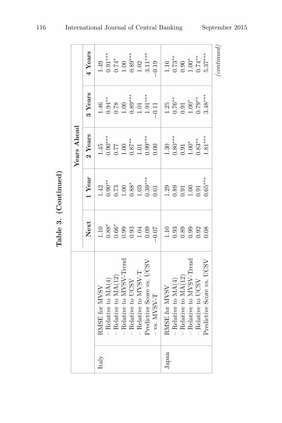
116 International Journal of Central Banking September 2015
Tab
le3.
(Con
tinued
)
Yea
rsA
hea
d
Nex
t1
Yea
r2
Yea
rs3
Yea
rs4
Yea
rs
Ital
yR
MSE
for
MV
SV1.
101.
421.
451.
461.
49–
Rel
ativ
eto
MA
(4)
0.88
∗0.
90∗∗
0.90
∗∗∗
0.94
∗∗0.
91∗∗
∗
–R
elat
ive
toM
A(1
2)0.
66∗
0.73
0.77
0.78
0.74
∗
–R
elat
ive
toM
VSV
-Tre
nd0.
991.
001.
001.
001.
00–
Rel
ativ
eto
UC
SV0.
930.
88∗
0.87
∗∗0.
89∗∗
∗0.
89∗∗
∗
–R
elat
ive
toM
VSV
-T1.
041.
031.
011.
011.
02P
redi
ctiv
eSc
ore
vs.U
CSV
0.09
0.39
∗∗∗
0.99
∗∗∗
1.91
∗∗∗
3.11
∗∗∗
–vs
.M
VSV
-T−
0.07
0.01
0.00
−0.
11−
0.19
Japa
nR
MSE
for
MV
SV1.
101.
291.
301.
251.
16–
Rel
ativ
eto
MA
(4)
0.93
0.89
0.80
∗∗∗
0.76
∗∗0.
73∗∗
–R
elat
ive
toM
A(1
2)0.
890.
910.
910.
910.
90–
Rel
ativ
eto
MV
SV-T
rend
0.99
1.00
1.00
∗1.
00∗
1.00
∗
–R
elat
ive
toU
CSV
0.92
0.91
0.83
∗∗0.
79∗∗
0.74
∗∗
Pre
dict
ive
Scor
evs
.U
CSV
0.08
0.65
∗∗∗
1.81
∗∗∗
3.48
∗∗∗
5.37
∗∗∗
(con
tinu
ed)

Vol. 11 No. S1 Trend Inflation in Advanced Economies 117
Tab
le3.
(Con
tinued
)
Yea
rsA
hea
d
Nex
t1
Yea
r2
Yea
rs3
Yea
rs4
Yea
rs
New
Zea
land
RM
SEfo
rM
VSV
3.08
3.51
3.85
4.49
4.87
–R
elat
ive
toM
A(4
)1.
081.
081.
101.
111.
11–
Rel
ativ
eto
MA
(12)
1.06
1.05
1.14
1.14
1.14
–R
elat
ive
toM
VSV
-Tre
nd1.
011.
001.
001.
001.
00–
Rel
ativ
eto
UC
SV0.
920.
94∗
0.96
0.97
0.99
–R
elat
ive
toM
VSV
-T1.
011.
021.
031.
021.
01P
redi
ctiv
eSc
ore
vs.U
CSV
0.14
∗∗∗
0.77
∗∗∗
1.98
∗∗∗
3.63
∗∗∗
5.53
∗∗∗
–vs
.M
VSV
-T0.
01−
0.28
∗∗∗
−0.
46∗∗
∗−
0.63
∗∗∗
−0.
78∗∗
∗
Swed
enR
MSE
for
MV
SV2.
032.
372.
712.
973.
13–
Rel
ativ
eto
MA
(4)
0.90
∗∗0.
870.
930.
940.
96–
Rel
ativ
eto
MA
(12)
0.88
∗∗∗
0.90
∗∗0.
981.
021.
02–
Rel
ativ
eto
MV
SV-T
rend
0.99
∗∗1.
001.
001.
001.
00–
Rel
ativ
eto
UC
SV0.
960.
890.
960.
960.
98–
Rel
ativ
eto
MV
SV-T
1.05
1.06
1.10
∗1.
091.
08P
redi
ctiv
eSc
ore
vs.U
CSV
0.15
∗∗∗
0.27
∗∗∗
0.78
∗∗∗
1.88
∗∗∗
3.37
∗∗∗
–vs
.M
VSV
-T−
0.06
−0.
13−
0.18
∗−
0.27
∗∗−
0.37
∗∗∗
(con
tinu
ed)
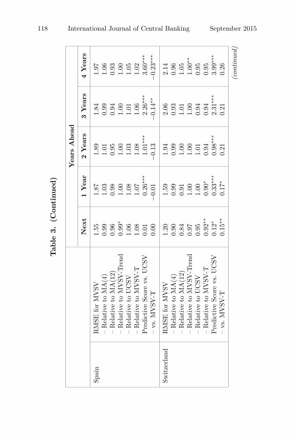
118 International Journal of Central Banking September 2015
Tab
le3.
(Con
tinued
)
Yea
rsA
hea
d
Nex
t1
Yea
r2
Yea
rs3
Yea
rs4
Yea
rs
Spai
nR
MSE
for
MV
SV1.
551.
871.
891.
841.
97–
Rel
ativ
eto
MA
(4)
0.99
1.03
1.01
0.99
1.06
–R
elat
ive
toM
A(1
2)0.
960.
980.
950.
940.
93–
Rel
ativ
eto
MV
SV-T
rend
0.99
∗1.
001.
001.
001.
00–
Rel
ativ
eto
UC
SV1.
061.
081.
031.
011.
05–
Rel
ativ
eto
MV
SV-T
1.08
1.07
1.08
1.06
1.02
Pre
dict
ive
Scor
evs
.U
CSV
0.01
0.26
∗∗∗
1.01
∗∗∗
2.26
∗∗∗
3.60
∗∗∗
–vs
.M
VSV
-T0.
00−
0.01
−0.
13−
0.14
∗∗−
0.23
∗∗∗
Swit
zerl
and
RM
SEfo
rM
VSV
1.20
1.59
1.94
2.06
2.14
–R
elat
ive
toM
A(4
)0.
900.
990.
990.
930.
96–
Rel
ativ
eto
MA
(12)
0.84
0.91
1.00
1.01
1.05
–R
elat
ive
toM
VSV
-Tre
nd0.
971.
001.
001.
001.
00∗∗
–R
elat
ive
toU
CSV
0.95
1.00
1.01
0.94
0.95
–R
elat
ive
toM
VSV
-T0.
92∗∗
0.90
∗0.
940.
940.
95P
redi
ctiv
eSc
ore
vs.U
CSV
0.12
∗0.
33∗∗
∗0.
98∗∗
∗2.
31∗∗
∗3.
99∗∗
∗
–vs
.M
VSV
-T0.
15∗∗
0.17
∗0.
210.
210.
26
(con
tinu
ed)

Vol. 11 No. S1 Trend Inflation in Advanced Economies 119
Tab
le3.
(Con
tinued
)
Yea
rsA
hea
d
Nex
t1
Yea
r2
Yea
rs3
Yea
rs4
Yea
rs
Uni
ted
Kin
gdom
RM
SEfo
rM
VSV
1.21
1.45
1.86
2.15
2.27
–R
elat
ive
toM
A(4
)0.
900.
850.
971.
031.
07–
Rel
ativ
eto
MA
(12)
0.85
0.86
1.02
1.13
1.12
–R
elat
ive
toM
VSV
-Tre
nd1.
021.
001.
001.
001.
00–
Rel
ativ
eto
UC
SV0.
850.
83∗
0.92
0.98
1.03
–R
elat
ive
toM
VSV
-T0.
93∗
0.94
0.97
1.00
1.01
Pre
dict
ive
Scor
evs
.U
CSV
0.04
0.53
∗∗∗
1.35
∗∗∗
2.69
∗∗∗
4.27
∗∗∗
–vs
.M
VSV
-T0.
11−
0.05
−0.
16−
0.22
∗−
0.29
∗∗
Uni
ted
Stat
esR
MSE
for
MV
SV1.
101.
221.
291.
341.
30–
Rel
ativ
eto
MA
(4)
0.71
∗∗0.
75∗∗
0.80
∗∗∗
0.79
∗∗∗
0.83
∗
–R
elat
ive
toM
A(1
2)0.
84∗∗
0.89
0.96
0.98
0.96
–R
elat
ive
toM
VSV
-Tre
nd1.
021.
001.
001.
001.
00–
Rel
ativ
eto
UC
SV0.
77∗∗
0.83
∗∗0.
82∗∗
∗0.
81∗∗
∗0.
79∗∗
–R
elat
ive
toM
VSV
-T1.
001.
001.
001.
001.
00P
redi
ctiv
eSc
ore
vs.U
CSV
0.32
∗∗∗
0.63
∗∗∗
1.27
∗∗∗
2.29
∗∗∗
3.57
∗∗∗
–vs
.M
VSV
-T−
0.00
0.00
−0.
000.
00−
0.00
(con
tinu
ed)

120 International Journal of Central Banking September 2015
Tab
le3.
(Con
tinued
)
Yea
rsA
hea
d
Nex
t1
Yea
r2
Yea
rs3
Yea
rs4
Yea
rs
Uni
ted
Stat
esR
MSE
for
MV
SV1.
141.
271.
321.
381.
38(C
PI-
U-R
S)–
Rel
ativ
eto
MA
(4)
0.69
∗∗0.
76∗∗
0.80
∗∗∗
0.80
∗∗0.
87–
Rel
ativ
eto
MA
(12)
0.82
∗∗0.
910.
981.
021.
03–
Rel
ativ
eto
MV
SV-T
rend
0.99
∗∗∗
1.00
1.00
1.00
1.00
–R
elat
ive
toU
CSV
0.84
∗∗0.
93∗
0.93
∗0.
940.
96–
Rel
ativ
eto
MV
SV-T
1.00
1.00
1.00
1.00
∗1.
00P
redi
ctiv
eSc
ore
vs.U
CSV
0.24
∗∗∗
0.31
∗∗∗
0.70
∗∗∗
1.70
∗∗∗
3.08
∗∗∗
–vs
.M
VSV
-T−
0.00
0.00
−0.
00−
0.00
∗∗−
0.00
Note
s:Fo
rea
chco
untr
y,ro
otm
ean
squa
red
erro
rs(R
MSE
)an
dav
erag
elo
g-pr
edic
tive
scor
esar
ede
rive
dfr
omou
t-of
-sam
ple
fore
cast
sth
atw
ere
gene
rate
dfr
omqu
asi-re
al-t
ime
esti
mat
esof
each
mod
elfr
om19
85:Q
1on
war
ds;
each
mod
eles
tim
atio
nis
cond
itio
ned
onda
tafr
om19
60:Q
1un
tilth
ebeg
inni
ngof
each
fore
cast
per
iod.
Super
scri
pts
*,**
,an
d**
*de
note
stat
isti
cally
sign
ifica
ntdi
ffer
ence
sin
squa
red
fore
cast
erro
rsan
dlo
g-pr
edic
tive
scor
es—
asco
mpu
ted
from
the
test
byD
iebol
dan
dM
aria
no(1
995)
—at
the
10per
cent
,5
per
cent
,an
d1
per
cent
leve
l,re
spec
tive
ly.

Vol. 11 No. S1 Trend Inflation in Advanced Economies 121
Tab
le4.
For
ecas
tEva
luat
ion:Q
uar
terl
yIn
flat
ion
Rat
es
Yea
rsA
hea
d
Nex
t1
Yea
r2
Yea
rs3
Yea
rs4
Yea
rs
Aus
tral
iaR
MSE
for
MV
SV2.
322.
543.
013.
243.
29–
Rel
ativ
eto
MA
(4)
0.96
0.92
∗0.
960.
980.
97–
Rel
ativ
eto
MA
(12)
0.92
0.92
1.02
1.07
1.04
–R
elat
ive
toM
VSV
-Tre
nd1.
011.
001.
001.
001.
00–
Rel
ativ
eto
UC
SV0.
960.
920.
950.
960.
96–
Rel
ativ
eto
MV
SV-T
1.04
1.09
∗∗1.
13∗∗
∗1.
10∗∗
1.07
∗∗
Pre
dict
ive
Scor
evs
.U
CSV
0.06
0.03
0.06
0.12
∗∗0.
39∗∗
∗
–vs
.M
VSV
-T−
0.03
−0.
06−
0.16
∗∗∗
−0.
20∗∗
∗−
0.22
∗∗
Bel
gium
RM
SEfo
rM
VSV
1.65
1.96
1.92
1.86
1.78
–R
elat
ive
toM
A(4
)0.
950.
920.
940.
990.
92–
Rel
ativ
eto
MA
(12)
0.89
∗0.
950.
990.
960.
99–
Rel
ativ
eto
MV
SV-T
rend
0.92
∗1.
001.
001.
001.
00–
Rel
ativ
eto
UC
SV1.
050.
950.
970.
970.
95–
Rel
ativ
eto
MV
SV-T
1.04
∗∗∗
1.06
∗∗∗
1.05
∗∗1.
001.
02P
redi
ctiv
eSc
ore
vs.U
CSV
−0.
080.
060.
16∗∗
0.22
∗∗0.
30∗∗
–vs
.M
VSV
-T−
0.08
∗∗−
0.06
∗0.
00−
0.01
−0.
05
(con
tinu
ed)
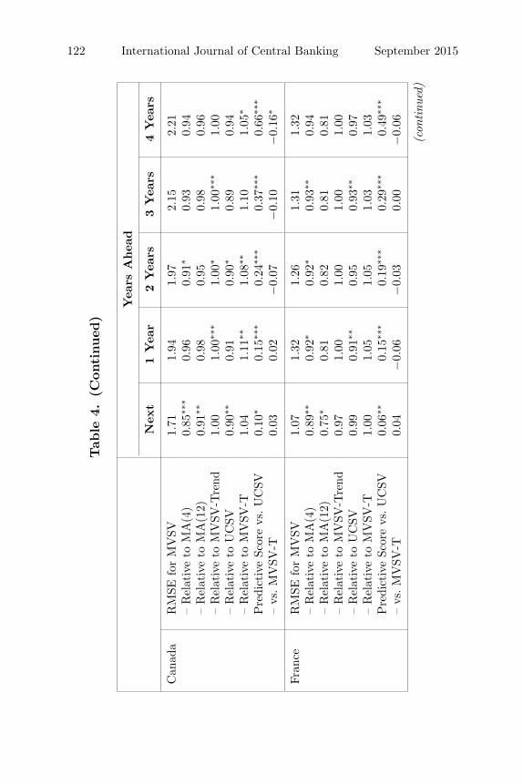
122 International Journal of Central Banking September 2015
Tab
le4.
(Con
tinued
)
Yea
rsA
hea
d
Nex
t1
Yea
r2
Yea
rs3
Yea
rs4
Yea
rs
Can
ada
RM
SEfo
rM
VSV
1.71
1.94
1.97
2.15
2.21
–R
elat
ive
toM
A(4
)0.
85∗∗
∗0.
960.
91∗
0.93
0.94
–R
elat
ive
toM
A(1
2)0.
91∗∗
0.98
0.95
0.98
0.96
–R
elat
ive
toM
VSV
-Tre
nd1.
001.
00∗∗
∗1.
00∗
1.00
∗∗∗
1.00
–R
elat
ive
toU
CSV
0.90
∗∗0.
910.
90∗
0.89
0.94
–R
elat
ive
toM
VSV
-T1.
041.
11∗∗
1.08
∗∗1.
101.
05∗
Pre
dict
ive
Scor
evs
.U
CSV
0.10
∗0.
15∗∗
∗0.
24∗∗
∗0.
37∗∗
∗0.
66∗∗
∗
–vs
.M
VSV
-T0.
030.
02−
0.07
−0.
10−
0.16
∗
Fran
ceR
MSE
for
MV
SV1.
071.
321.
261.
311.
32–
Rel
ativ
eto
MA
(4)
0.89
∗∗0.
92∗
0.92
∗0.
93∗∗
0.94
–R
elat
ive
toM
A(1
2)0.
75∗
0.81
0.82
0.81
0.81
–R
elat
ive
toM
VSV
-Tre
nd0.
971.
001.
001.
001.
00–
Rel
ativ
eto
UC
SV0.
990.
91∗∗
0.95
0.93
∗∗0.
97–
Rel
ativ
eto
MV
SV-T
1.00
1.05
1.05
1.03
1.03
Pre
dict
ive
Scor
evs
.U
CSV
0.06
∗∗0.
15∗∗
∗0.
19∗∗
∗0.
29∗∗
∗0.
49∗∗
∗
–vs
.M
VSV
-T0.
04−
0.06
−0.
030.
00−
0.06
(con
tinu
ed)

Vol. 11 No. S1 Trend Inflation in Advanced Economies 123
Tab
le4.
(Con
tinued
)
Yea
rsA
hea
d
Nex
t1
Yea
r2
Yea
rs3
Yea
rs4
Yea
rs
Ger
man
yR
MSE
for
MV
SV1.
461.
661.
831.
892.
00–
Rel
ativ
eto
MA
(4)
1.01
0.98
0.96
0.94
0.92
–R
elat
ive
toM
A(1
2)0.
920.
930.
960.
930.
94–
Rel
ativ
eto
MV
SV-T
rend
0.99
1.00
1.00
1.00
1.00
–R
elat
ive
toU
CSV
1.01
0.98
0.94
0.93
0.92
–R
elat
ive
toM
VSV
-T1.
021.
061.
05∗
1.02
1.02
Pre
dict
ive
Scor
evs
.U
CSV
−0.
010.
030.
070.
12∗∗
∗0.
15∗∗
∗
–vs
.M
VSV
-T−
0.03
−0.
09∗∗
−0.
10∗∗
−0.
09∗
−0.
12∗
Irel
and
RM
SEfo
rM
VSV
1.97
3.03
3.33
3.34
3.00
–R
elat
ive
toM
A(4
)0.
87∗∗
0.96
0.98
1.00
1.00
–R
elat
ive
toM
A(1
2)0.
73∗∗
0.98
1.09
1.13
1.04
–R
elat
ive
toM
VSV
-Tre
nd1.
001.
001.
001.
001.
00–
Rel
ativ
eto
UC
SV1.
050.
950.
920.
940.
94–
Rel
ativ
eto
MV
SV-T
0.88
∗1.
131.
271.
22∗
1.10
Pre
dict
ive
Scor
evs
.U
CSV
0.00
0.24
0.12
0.04
0.04
–vs
.M
VSV
-T0.
07−
0.14
−0.
090.
040.
13
(con
tinu
ed)

124 International Journal of Central Banking September 2015
Tab
le4.
(Con
tinued
)
Yea
rsA
hea
d
Nex
t1
Yea
r2
Yea
rs3
Yea
rs4
Yea
rs
Ital
yR
MSE
for
MV
SV1.
061.
491.
601.
641.
58–
Rel
ativ
eto
MA
(4)
0.89
∗0.
91∗
0.90
∗∗∗
0.93
∗∗∗
0.95
∗∗
–R
elat
ive
toM
A(1
2)0.
67∗∗
∗0.
750.
780.
810.
80–
Rel
ativ
eto
MV
SV-T
rend
0.96
∗∗1.
001.
001.
001.
00–
Rel
ativ
eto
UC
SV1.
040.
900.
88∗
0.89
∗∗0.
92∗∗
∗
–R
elat
ive
toM
VSV
-T1.
011.
031.
011.
001.
01P
redi
ctiv
eSc
ore
vs.U
CSV
0.03
0.12
∗0.
24∗∗
∗0.
39∗∗
∗0.
62∗∗
∗
–vs
.M
VSV
-T−
0.01
−0.
07∗∗
−0.
020.
00−
0.08
Japa
nR
MSE
for
MV
SV1.
631.
751.
881.
851.
82–
Rel
ativ
eto
MA
(4)
0.97
0.96
0.94
0.90
∗0.
83∗∗
∗
–R
elat
ive
toM
A(1
2)0.
960.
960.
970.
960.
97–
Rel
ativ
eto
MV
SV-T
rend
0.99
1.00
1.00
1.00
1.00
–R
elat
ive
toU
CSV
0.99
0.94
0.95
0.90
∗∗0.
86∗∗
∗
Pre
dict
ive
Scor
evs
.U
CSV
−0.
020.
12∗
0.30
∗∗∗
0.92
∗∗∗
2.03
∗∗∗
(con
tinu
ed)

Vol. 11 No. S1 Trend Inflation in Advanced Economies 125
Tab
le4.
(Con
tinued
)
Yea
rsA
hea
d
Nex
t1
Yea
r2
Yea
rs3
Yea
rs4
Yea
rs
New
Zea
land
RM
SEfo
rM
VSV
3.53
4.29
4.60
4.36
4.82
–R
elat
ive
toM
A(4
)0.
961.
131.
081.
061.
09–
Rel
ativ
eto
MA
(12)
0.96
1.08
1.09
1.12
1.11
–R
elat
ive
toM
VSV
-Tre
nd1.
031.
00∗
1.00
1.00
1.00
–R
elat
ive
toU
CSV
0.94
0.94
∗0.
970.
960.
98–
Rel
ativ
eto
MV
SV-T
1.00
1.02
∗∗1.
021.
021.
02P
redi
ctiv
eSc
ore
vs.U
CSV
0.11
∗∗∗
0.11
∗∗∗
0.21
∗∗∗
0.42
∗∗∗
0.95
∗∗∗
–vs
.M
VSV
-T0.
03−
0.09
−0.
24∗∗
∗−
0.37
∗∗∗
−0.
43∗∗
∗
Swed
enR
MSE
for
MV
SV2.
462.
873.
073.
363.
50–
Rel
ativ
eto
MA
(4)
0.97
0.93
0.93
0.95
0.96
–R
elat
ive
toM
A(1
2)0.
90∗∗
∗0.
94∗
0.95
1.01
1.02
–R
elat
ive
toM
VSV
-Tre
nd0.
981.
001.
001.
001.
00–
Rel
ativ
eto
UC
SV1.
000.
95∗
0.93
0.97
0.97
–R
elat
ive
toM
VSV
-T1.
031.
031.
051.
071.
06P
redi
ctiv
eSc
ore
vs.U
CSV
0.07
0.12
∗∗∗
0.11
∗∗∗
0.13
∗∗∗
0.18
∗∗∗
–vs
.M
VSV
-T−
0.00
−0.
06−
0.10
∗∗−
0.15
∗∗∗
−0.
19∗∗
∗
(con
tinu
ed)

126 International Journal of Central Banking September 2015
Tab
le4.
(Con
tinued
)
Yea
rsA
hea
d
Nex
t1
Yea
r2
Yea
rs3
Yea
rs4
Yea
rs
Spai
nR
MSE
for
MV
SV1.
872.
172.
332.
222.
21–
Rel
ativ
eto
MA
(4)
0.98
1.00
1.02
0.97
1.02
–R
elat
ive
toM
A(1
2)0.
941.
000.
980.
960.
94–
Rel
ativ
eto
MV
SV–T
rend
0.97
∗∗∗
1.00
1.00
1.00
1.00
–R
elat
ive
toU
CSV
1.03
1.03
1.03
1.00
1.01
–R
elat
ive
toM
VSV
–T1.
031.
041.
041.
071.
02P
redi
ctiv
eSc
ore
vs.U
CSV
0.01
0.04
0.08
∗0.
31∗∗
∗0.
67∗∗
∗
–vs
.M
VSV
–T0.
00−
0.02
−0.
04−
0.09
∗−
0.10
∗∗∗
Swit
zerl
and
RM
SEfo
rM
VSV
1.26
1.71
1.90
2.22
2.29
–R
elat
ive
toM
A(4
)0.
87∗∗
0.98
0.98
0.98
0.94
–R
elat
ive
toM
A(1
2)0.
81∗∗
0.94
0.93
1.02
1.02
–R
elat
ive
toM
VSV
–Tre
nd0.
93∗
1.00
1.00
1.00
1.00
∗
–R
elat
ive
toU
CSV
0.95
0.96
0.98
0.99
0.95
–R
elat
ive
toM
VSV
–T0.
980.
93∗
0.92
∗0.
950.
95P
redi
ctiv
eSc
ore
vs.U
CSV
0.07
∗∗∗
0.10
∗∗0.
18∗∗
0.57
∗∗∗
1.52
∗∗∗
–vs
.M
VSV
–T0.
040.
08∗
0.12
0.18
0.13
(con
tinu
ed)

Vol. 11 No. S1 Trend Inflation in Advanced Economies 127
Tab
le4.
(Con
tinued
)
Yea
rsA
hea
d
Nex
t1
Yea
r2
Yea
rs3
Yea
rs4
Yea
rs
Uni
ted
Kin
gdom
RM
SEfo
rM
VSV
1.65
1.75
2.06
2.24
2.53
–R
elat
ive
toM
A(4
)0.
970.
950.
930.
981.
06–
Rel
ativ
eto
MA
(12)
0.92
0.91
0.99
1.03
1.13
–R
elat
ive
toM
VSV
-Tre
nd1.
021.
001.
001.
001.
00–
Rel
ativ
eto
UC
SV0.
960.
89∗
0.90
∗∗0.
960.
99–
Rel
ativ
eto
MV
SV-T
0.99
0.94
∗∗0.
990.
981.
00P
redi
ctiv
eSc
ore
vs.U
CSV
0.04
0.09
∗0.
21∗∗
∗0.
37∗∗
∗0.
72∗∗
∗
–vs
.M
VSV
-T0.
020.
04−
0.12
−0.
15∗
−0.
21∗∗
Uni
ted
Stat
esR
MSE
for
MV
SV1.
771.
891.
881.
982.
00–
Rel
ativ
eto
MA
(4)
0.85
∗∗0.
88∗
0.85
∗0.
91∗∗
∗0.
87∗∗
–R
elat
ive
toM
A(1
2)0.
92∗∗
0.95
0.94
1.00
0.99
–R
elat
ive
toM
VSV
-Tre
nd0.
981.
001.
001.
001.
00–
Rel
ativ
eto
UC
SV0.
93∗
0.87
∗∗0.
90∗∗
0.91
∗∗0.
88∗∗
∗
–R
elat
ive
toM
VSV
-T1.
001.
001.
001.
001.
00P
redi
ctiv
eSc
ore
vs.U
CSV
0.13
∗∗0.
21∗∗
∗0.
230.
290.
37∗
–vs
.M
VSV
-T0.
00−
0.00
−0.
00−
0.00
−0.
00
(con
tinu
ed)

128 International Journal of Central Banking September 2015
Tab
le4.
(Con
tinued
)
Yea
rsA
hea
d
Nex
t1
Yea
r2
Yea
rs3
Yea
rs4
Yea
rs
Uni
ted
Stat
esR
MSE
for
MV
SV2.
632.
692.
722.
782.
85(C
PI-
U-R
S)–
Rel
ativ
eto
MA
(4)
0.87
∗∗∗
0.91
∗∗0.
920.
92∗∗
∗0.
92∗∗
–R
elat
ive
toM
A(1
2)0.
93∗∗
∗0.
94∗∗
∗0.
97∗∗
0.98
0.99
–R
elat
ive
toM
VSV
-Tre
nd0.
970.
98∗∗
∗0.
99∗∗
∗1.
00∗∗
∗1.
00∗∗
–R
elat
ive
toU
CSV
0.91
∗∗∗
0.97
∗∗0.
990.
991.
00–
Rel
ativ
eto
MV
SV-T
1.00
1.00
1.00
1.00
1.00
∗
Pre
dict
ive
Scor
evs
.U
CSV
0.15
∗∗∗
0.02
0.04
0.02
0.07
–vs
.M
VSV
-T0.
00−
0.00
0.00
0.00
0.00
Note
s:Fo
rea
chco
untr
y,ro
otm
ean
squa
red
erro
rs(R
MSE
)an
dav
erag
elo
g-pr
edic
tive
scor
esar
ede
rive
dfr
omou
t-of
-sam
ple
fore
cast
sth
atw
ere
gene
rate
dfr
omqu
asi-re
al-t
ime
esti
mat
esof
each
mod
elfr
om19
85:Q
1on
war
ds;
each
mod
eles
tim
atio
nis
cond
itio
ned
onda
tafr
om19
60:Q
1un
tilth
ebeg
inni
ngof
each
fore
cast
per
iod.
Super
scri
pts
*,**
,an
d**
*de
note
stat
isti
cally
sign
ifica
ntdi
ffer
ence
sin
squa
red
fore
cast
erro
rsan
dlo
g-pr
edic
tive
scor
es—
asco
mpu
ted
from
the
test
byD
iebol
dan
dM
aria
no(1
995)
—at
the
10per
cent
,5
per
cent
,an
d1
per
cent
leve
l,re
spec
tive
ly.
Vol. 11 No. S1 Trend Inflation in Advanced Economies 129
RMSE ratio indicates that the MVSV model has a lower RMSE,and conversely for values above unity. A positive value for the dif-ference in the average log-predictive scores indicates a more accuratepredictive density of the MVSV value, with the converse holding inthe case of a negative value for the difference. The statistical signifi-cance of the differences in RMSE and log-predictive scores is assessedwith the Diebold-Mariano (1995) test.31
Several results recur across both tables. First, with only a coupleof exceptions, the MVSV model generates lower RMSE for almosteach country and at almost each horizon than a simple random-walkforecast. Second, in most countries, the same is also true, but often toa lesser extent, when the MVSV forecasts are compared with thoseof the UCSV model. Third, although most of these differences arenotable—in the neighborhood of several tenths of the MVSV model’sRMSEs—they are often not statistically significant. Primarily in thecases of France, Italy, and the United States, the MVSV model pro-duces forecasts that are significantly better than projections derivedfrom either a random-walk or UCSV model. Strikingly, the MVSVmodel rarely fares significantly worse than any of the moving aver-ages or the UCSV model. The MVSV model also generates consider-ably higher log-predictive scores than the UCSV, suggesting a moreaccurate predictive density, especially over longer forecast horizons.To quite some extent, this reflects the differences in specificationof the stochastic volatilities for the inflation gaps. As described insection 3, the UCSV model embeds the assumption that the logof the inflation-gap shock variance follows a random walk whereasthe MVSV model uses an AR(1) specification. At longer forecasthorizons, the random-walk assumption for the inflation-gap vari-ance seems to lead to undue extrapolation of temporary changes involatility—a property that has an adverse bearing on the accuracyof the UCSV model’s predictive density.
Comparison of the absolute levels of the RMSEs for the MVSVmodel across both tables shows that RMSE values are somewhat
31The Diebold-Mariano (1995) test is designed to ascertain whether the squaredlosses generated by two different forecasts are, on average, equal. In light ofthe overlap in the forecast periods, we computed the standard errors using theNewey-West (1997) robust estimator, with a bandwidth set equal to one plus theforecast horizon. The Diebold-Mariano test can also be used to assess differencesin log-predictive scores, as recently shown by Clark and Ravazzolo (2014).
130 International Journal of Central Banking September 2015
larger for cases in which it is the quarterly rather than annualrate of inflation that is being forecast. This pattern is indicativeof the considerable amount of highly transitory—and hence harderto forecast—fluctuations found in quarter-to-quarter variations inprices. These variations figure less heavily in the behavior of four-quarter inflation, a series in which the most violent swings in quar-terly inflation are averaged out by construction. Correspondingly,the differences in RMSEs across the different models, which areclearly evident in the quarterly inflation results in table 4, are smallerin size and tend to be less statistically significant when forecastsof annual inflation are considered, as in table 3; a similar patternholds also for differences in log-predictive scores between MVSVand UCSV model.
We also consider the forecasting performance of the MVSV trendalone, neglecting the horizon-specific information resulting from theVAR component of the model’s gap equation (for a given trend-inflation estimate). In this case, forecasts for all horizons are setequal to the models’ trend estimate, generated in quasi-real time(and shown in figure 18). For projections of both quarterly andannual inflation—reported in tables 3 and 4—there is typically nota great difference between the (average) forecast errors arising fromthe MVSV model (from which inflation forecasts are derived fromsumming the inflation-trend forecast and the inflation-gap forecast)and the errors of inflation projections derived from relying solely onthe MVSV-generated inflation trend. This finding is consistent withthe notion, espoused by Faust and Wright (2013), that improvedforecast accuracy stems from the quality of the estimates of theinflation trend. Applied to the MVSV approach, this notion impliesthat the model’s VAR equation for the inflation gap adds little valuebeyond its role in shaping the trend estimate itself.
For the United States, the MVSV model tends to outperformeither a random-walk or the UCSV model, both in terms of RMSEand predictive density score, and significantly so in most cases.Results are fairly similar when using either the regular CPI or theCPI-U-RS measure, as table 3 shows.
As a final comparison, we consider forecasts from the MVSV-Tmodel that sets the inflation trend equal to each country’s infla-tion goal when applicable. In contrast to the baseline MVSV model,the MVSV-T model does not centers its forecasts on an empirical
Vol. 11 No. S1 Trend Inflation in Advanced Economies 131
trend estimate. Instead, it takes the trend as corresponding toeach country’s official inflation goal (when applicable). Furthermore,once an inflation goal has been introduced for a given country, theMVSV-T model treats the inflation trend as deterministic, thusremoving uncertainty about future trend shocks from the predictivedensity.32 The forecast performance of the MVSV-T model com-pared with the MVSV model differs for different countries. In sev-eral instances, like those of Australia, Canada, and New Zealand,conditioning on a known inflation goal clearly improves forecastsboth in terms of RMSE and predictive density, especially for longerforecast horizons. In other cases, like Switzerland and Ireland, theopposite is true, although the differences are not statistically sig-nificant. For several countries—including France, Belgium, and theUnited States—forecasts derived from the MVSV-T model do notdiffer greatly from those generated by the baseline version of theMVSV model.33 If anything, the predictive density of longer-horizonforecasts tends to be improved when generated from the MVSV-Tmodel.
8. Conclusion
Our paper has compared estimates of trend inflation in fourteenadvanced economies using two different models. Our preferred modelis a multivariate extension of Stock and Watson’s (2007) unobserved-components model with stochastic volatility (UCSV) that has beenapplied to the G7 countries by Cecchetti et al. (2007). Like the UCSVmodel, our multivariate stochastic volatility model (MVSV) trackstime variation in the variability of shocks to trend inflation and theinflation gap. Inflation-gap estimates from our MVSV model allowfor inflation-gap persistence—albeit modeled in a more parsimoniousfashion than in Cogley, Primiceri, and Sargent (2010)—while theUCSV model embeds the assumption that gaps are serially uncorre-lated. We find that, particularly since the 1980s, the MVSV-based
32At a given point in time, future adjustments in the inflation goal are, however,not anticipated by the MVSV-T model.
33In the case of the United States, forecasts from the MVSV and the MVSV-Tmodel barely differ, on average, from each other in part also because of the lim-ited number of observations for which the Federal Reserve’s longer-term inflationobjective, officially introduced in 2012, applies in our sample.

132 International Journal of Central Banking September 2015
inflation trends are smoother and less variable than their UCSVcounterparts, as the underlying filtering procedure implies less influ-ence on the trend estimates of persistent variations in inflation thatdo not prove to be fully permanent.
A key additional property of the MVSV model is that it condi-tions on multiple inflation series, on the assumption that they sharea common trend, as in the model of Mertens (2011). In contrastto Cogley and Sargent (2005), Kang, Kim, and Morley (2009), andCogley, Primiceri, and Sargent (2010), our model restricts time vari-ation in inflation-gap parameters only to the evolution of stochasticvolatility. This variation is in turn limited to only two sources: driftin the log-variances of shocks to the common trend and separate,but cross-correlated, volatility processes for each inflation gap. Plac-ing a limit in this way on the number of time-varying parametersmakes the model more tractable, and it also enables us to handlemissing data in some of the inflation series for several countries,while still allowing for the possibility of considerable persistence inthe inflation-gap series. This restricted approach also holds out theprospect of greater forecast accuracy. Compared with alternativeforecasts—generated either from a simple random-walk model orthe UCSV model—our MVSV model typically is associated witha lower average size of forecast errors at various horizons and formost countries. In particular, for the exercise of forecasting four-quarter inflation rates (as distinct from quarter-to-quarter rates),the improvements are quite appreciable. However, with the excep-tion of a few countries, it remains hard to generate inflation forecaststhat outperform random-walk forecasts of inflation by a statisticallysignificant amount.
Although our estimates of trend inflation display quite some sim-ilarities across countries—notably the shared experiences of persis-tently elevated values during the 1970s and more reliably anchoredinflation expectations over the last two decades—there are alsoclear cross-country differences in the trend estimates. For example,the extent to which trend inflation underwent a rise, and subse-quent fall, over the post-war sample differs notably across countries.In addition, for many countries, distinct, country-specific changesin monetary regime, like the adoption of a formal inflation tar-get, are clearly visible in the evolution of our estimates of trendinflation.
Vol. 11 No. S1 Trend Inflation in Advanced Economies 133
References
Adolfson, M., J. Linde, and M. Villani. 2007. “Forecasting Per-formance of an Open Economy DSGE Model.” EconometricReviews 26 (2–4): 289–328.
Atkeson, A., and L. E. Ohanian. 2001. “Are Phillips Curves Usefulfor Forecasting Inflation?” Quarterly Review (Federal ReserveBank of Minneapolis) 25 (1): 2–11.
Bernanke, B. S., T. L. Laubach, F. S. Mishkin, and A. S. Posen. 1999.Inflation Targeting: Lessons from the International Experience.Princeton, NJ: Princeton University Press.
Berstein, S. 1993. The Republic of de Gaulle, 1958–1969. Cambridge,UK: Cambridge University Press.
Beveridge, S., and C. R. Nelson. 1981. “A New Approach to Decom-position of Economic Time Series into Permanent and TransitoryComponents with Particular Attention to Measurement of the‘Business Cycle’.” Journal of Monetary Economics 7 (2): 151–74.
Braun, A. R. 1986. Wage Determination and Incomes Policy in OpenEconomies. Washington, DC: International Monetary Fund.
Cecchetti, S. G., P. Hooper, B. C. Kasman, K. L. Schoenholtz,and M. W. Watson. 2007. “Understanding the Evolving Infla-tion Process.” Presented for the U.S. Monetary Policy Forum onMarch 9, 2007, sponsored by the Initiative on Global Marketsat the University of Chicago Booth School of Business; revisedversion, July.
Ciccarelli, M., and B. Mojon. 2010. “Global Inflation.” Review ofEconomics and Statistics 92 (3): 524–35.
Clark, T. E., and T. Doh. 2011. “A Bayesian Evaluation of Alterna-tive Models of Trend Inflation.” Working Paper No. 1134, FederalReserve Bank of Cleveland.
Clark, T. E., and F. Ravazzolo. 2014. “Macroeconomic ForecastingPerformance under Alternative Specifications of Time-VaryingVolatility.” Forthcoming in Journal of Applied Econometrics.
Cogley, T., G. E. Primiceri, and T. J. Sargent. 2010. “Inflation-GapPersistence in the U.S.” American Economic Journal: Macroeco-nomics 2 (1): 43–69.
Cogley, T., and T. J. Sargent. 2005. “Drifts and Volatilities: Mone-tary Policies and Outcomes in the Post-WWII U.S.” Review ofEconomic Dynamics 8 (2): 262–302.
134 International Journal of Central Banking September 2015
———. 2015. “Measuring Price-Level Uncertainty and Stability inthe U.S., 1850–2012.” Forthcoming in Review of Economics andStatistics.
Cogley, T., T. J. Sargent, and P. Surico. 2014. “Price-Level Uncer-tainty and Stability in the United Kingdom.” Manuscript, NewYork University (November).
Cogley, T., and A. M. Sbordone. 2008. “Trend Inflation, Indexation,and Inflation Persistence in the New Keynesian Phillips Curve.”American Economic Review 98 (5): 2101–26.
Debelle, G., and J. Wilkinson. 2002. “Inflation Targeting andthe Inflation Process: Some Lessons from an Open Economy.”Research Discussion Paper No. 2002–01, Reserve Bank of Aus-tralia.
Diebold, F. X., and R. S. Mariano. 1995. “Comparing PredictiveAccuracy.” Journal of Business and Economic Statistics 13 (3):253–63.
Faust, J., and J. H. Wright. 2013. “Forecasting Inflation.” In Hand-book of Economic Forecasting, Vol. 2A, ed. G. A. Elliot and A.Timmermann, 3–56. New York: Elsevier.
Gelman, A., and D. B. Rubin. 1992. “Inference from Iterative Simu-lation Using Multiple Sequences.” Statistical Science 7 (4): 457–72.
Gordon, R. J. 1983. “A Century of Evidence on Wage and PriceStickiness in the United States, the United Kingdom, andJapan.” In Macroeconomics, Prices, and Quantities: Essays inMemory of Arthur M. Okun, ed. J. Tobin, 85–133. Washington,DC: Brookings Institution.
Grassi, S., and T. Proietti. 2010. “Has the Volatility of U.S. InflationChanged and How? Journal of Time Series Econometrics 2 (1):1–22.
Harvey, A. C. 1989. Forecasting, Structural Time Series Models andthe Kalman Filter. Cambridge, UK: Cambridge University Press.
Ireland, P. N. 2007. “Changes in the Federal Reserve’s Inflation Tar-get: Causes and Consequences.” Journal of Money, Credit andBanking 39 (8): 1851–82.
Kang, K. H., C.-J. Kim, and J. Morley. 2009. “Changes in U.S.Inflation Persistence.” Studies in Nonlinear Dynamic and Econo-metrics 13 (4): 1–21.
Vol. 11 No. S1 Trend Inflation in Advanced Economies 135
Klitgaard, T., and R. Peck. 2014. “High Unemployment and Disin-flation in the Euro Area Periphery Countries.” Liberty StreetEconomics Blog Entry, July 14. Available at http://libertystreeteconomics.newyorkfed.org/2014/07/high-unemployment-and-disinflation-in-the-euro-area-periphery-countries.html.
Kozicki, S., and P. A. Tinsley. 2012. “Effective Use of Survey Infor-mation in Estimating the Evolution of Expected Inflation.” Jour-nal of Money, Credit and Banking 44 (1): 145–69.
Levin, A. T., and J. M. Piger. 2004. “Is Inflation Persistence Intrinsicin Industrial Economies?” ECB Working Paper No. 334.
Mertens, E. 2011. “Measuring the Level of Uncertainty of TrendInflation.” Finance and Economics Discussion Series Paper No.42, Board of Governors of the Federal Reserve System.
Morley, J. 2011. “The Two Interpretations of the Beveridge–NelsonDecomposition.” Macroeconomic Dynamics 15 (3): 419–39.
Morley, J., J. M. Piger, and R. H. Rasche. 2015. “Inflation in the G7:Mind the Gap(s).” Macroeconomic Dynamics 19 (Special Issue04): 883–912.
Mumtaz, H., S. Simonelli, and P. Surico. 2011. “InternationalComovements, Business Cycle and Inflation: A Historical Per-spective.” Review of Economic Dynamics 14 (1): 176–98.
Mumtaz, H., and P. Surico. 2009. “The Transmission of Interna-tional Shocks: A Factor-Augmented VAR Approach.” Journal ofMoney, Credit and Banking 41 (s1): 71–100.
———. 2012. “Evolving International Inflation Dynamics: Worldand Country-Specific Factors.” Journal of the European Eco-nomic Association 10 (4): 716–34.
Neiss, K. S., and E. Nelson. 2005. “Inflation Dynamics, MarginalCost, and the Output Gap: Evidence from Three Countries.”Journal of Money, Credit and Banking 37 (6): 1019–45.
Newey, W. K., and K. D. West. 1987. “A Simple, PositiveSemi-Definite, Heteroskedasticity and Autocorrelation Consis-tent Covariance Matrix.” Econometrica 55 (3): 703–8.
Orphanides, A., and S. van Norden. 2002. “The Unreliability ofOutput-Gap Estimates in Real Time.” Review of Economics andStatistics 84 (4): 569–83.
Salin, P., and G. Lane. 1977. “Inflation in France.” In WorldwideInflation: Theory and Recent Experience, ed. L. B. Krause andW. S. Salant, 545–84. Washington, DC: Brookings Institution.

136 International Journal of Central Banking September 2015
Staiger, D. O., J. H. Stock, and M. W. Watson. 1997. “How PreciseAre Estimates of the Natural Rate of Unemployment?” In Reduc-ing Inflation: Motivation and Strategy, ed. C. D. Romer and D.H. Romer, 195–246. Chicago: University of Chicago Press.
Stock, J. H., and M. W. Watson. 2003. “Forecasting Output andInflation: The Role of Asset Prices.” Journal of Economic Liter-ature 41 (3): 788–829.
———. 2007. “Why Has U.S. Inflation Become Harder to Forecast?”Journal of Money, Credit and Banking 39 (s1): 3–33.
———. 2009. “Phillips Curve Inflation Forecasts.” In UnderstandingInflation and the Implications for Monetary Policy: A PhillipsCurve Retrospective, ed. J. C. Fuhrer, Y. K. Kodrzycki, J. S.Little, and G. P. Olivei, 99–184. Cambridge, MA: MIT Press.
———. 2010. “Modeling Inflation after the Crisis.” In Macroeco-nomic Challenges: The Decade Ahead, ed. Federal Reserve Bankof Kansas City, 173–220. Kansas City, MO: Federal Reserve Bankof Kansas City.
Svensson, L. E. O. 2015. “The Possible Unemployment Cost ofAverage Inflation below a Credible Target.” American EconomicJournal: Macroeconomics 7 (1): 258–96.
Ungerer, H. 1997. A Concise History of European Monetary Inte-gration: From EPU to EMU. Westport, CT: Quorum Books.
Wright, J. H. 2011. “Term Premia and Inflation Uncertainty: Empir-ical Evidence from an International Panel Dataset.” AmericanEconomic Review 101 (4): 1514–34.