trend following, risk parity and momentum in commodity futures
TRANSCRIPT

International Review of Financial Analysis 31 (2014) 1–12
Contents lists available at ScienceDirect
International Review of Financial Analysis
Trend following, risk parity and momentum in commodity futures
Andrew Clare a, James Seaton a, Peter N. Smith b, Stephen Thomas a,⁎a Cass Business School, City University London, 106 Bunhill Row, London EC1Y 8TZ, UKb Department of Economics, University of York, YO10 5DD, UK
⁎ Corresponding author.E-mail address: [email protected] (S. Thom
1057-5219/$ – see front matter © 2013 Elsevier Inc. All rihttp://dx.doi.org/10.1016/j.irfa.2013.10.001
a b s t r a c t
a r t i c l e i n f oArticle history:Received 31 January 2013Received in revised form 19 July 2013Accepted 4 October 2013Available online 22 October 2013
JEL classification:G12G13G15F65
Keywords:Trend followingMomentumRisk parityEqually-weightedPortfoliosCommodity futures
Weshow that combiningmomentumand trend following strategies for individual commodity futures can lead toportfolios which offer attractive risk adjusted returns which are superior to simple momentum strategies; whenwe expose these returns to a wide array of sources of systematic risk we find that robust alpha survives.Experimenting with risk parity portfolio weightings has limited impact on our results though in particular isbeneficial to long–short strategies; the marginal impact of applying trend following methods far outweighsmomentum and risk parity adjustments in terms of risk-adjusted returns and limiting downside risk. Overallthis leads to an attractive strategy for investing in commodity futures and emphasises the importance of trendfollowing as an investment strategy in the commodity futures context.
© 2013 Elsevier Inc. All rights reserved.
1. Introduction
The benefits of investing in commodities as an asset class both as aportfolio diversifier and as an inflation hedge have been increasingly ofinterest to academics and investors especially since the wide-rangingstudy by Gorton and Rouwenhorst (2006). However, investment incommodities is not straightforward and is generally accessed in financialmarkets by liquid futures' contracts traded on organised exchanges. Inthis paper we contribute to the growing evidence that applying a trendfollowing investment strategy to a variety of asset classes leads toenhanced risk adjusted returns. In particular we show that combiningmomentum and trend following strategies for individual commodityfutures can lead to portfolios which offer attractive risk adjusted returns;when we expose these returns to a wide array of sources of systematicrisk we find that robust alpha survives. Experimenting with risk parityportfolio weightings has limited impact on our results though it isbeneficial to long–short strategies; the marginal benefit of applyingtrend following methods far outweighs momentum and risk parityadjustments in terms of risk-adjusted returns and limiting downsiderisk.
Momentum strategies involve ranking assets based on their pastreturn (often the previous twelvemonths) and then buying thewinners
as).
ghts reserved.
and selling the losers. Momentum is one anomaly in the financialliterature that has been demonstrated to offer enhanced future returns.Many studies since Jegadeesh and Titman (1993) have focussed onmomentum at the individual stock level. More recently Asness,Moskowitz, and Pedersen (2013) find momentum effects within awide variety of asset classes. In terms of commodity futures, Miffreand Rallis (2007) and Erb and Harvey (2006) were amongst the firstto show that momentum strategies earn significant positive excessreturns. The purpose of this paper is to showhowamomentumstrategyfor commodity futures which also employs a trend following overlaycan significantly enhance investment performance relative to bothlong only and long–short momentum strategies.
Trend following has been widely used in futures markets,particularly commodities, for many decades (see Ostgaard, 2008).Trading signals can be generated by a variety of methods such asmoving average crossovers and breakouts with the aim of determiningthe trend in prices. Long positions are adopted when the trend ispositive and short positions, or cash, are taken when the trend isnegative. As trend following is generally rule-based it can aid investorssince losses are mechanically cut short and winners left to run. This isfrequently the reverse of investors' natural instincts. The return oncash (in this case the 3-month US Treasury Bill rate) is also an importantfactor either as collateral in futures or as the risk-off asset for long-onlymethods. Examples of the effectiveness of trend following forcommodity futures, amongst others, are Szakmary, Shen, and Sharma

2 An example of a provider of commodity ETF's based on the indices analysed in thispaper is ETF Securities, http://www.etfsecurities.com/institutional/uk/en-gb/products.aspx.
3 Anexplanation of thepractical issues involved in rolling returns can be foundat http://www.followingthetrend.com/futures-charts/futures-data-adjustments/.
2 A. Clare et al. / International Review of Financial Analysis 31 (2014) 1–12
(2010) and Hurst, Johnson, and Ooi (2010); Hurst, Ooi, and Pedersen(2010). As withmomentum strategies, much of the research is focussedon equities with Wilcox and Crittenden (2005) and ap Gwilym, Clare,Seaton, and Thomas (2010) as examples. Recent attempts at explainingthe success of trend following include Faber (2007) who uses trendfollowing as a means of tactical asset allocation and demonstrates thatit is possible to form a portfolio that has equity-level returns withbond-level volatility. Ilmanen (2011) offers a variety of explanationsas to why trend following may have been successful historically,including investor under-reaction to news and herding behaviour.
A few studies have sought to combine the momentum and trend-following strategies in equities. Faber (2010) examines momentumand a form of trend following in equity sector investing in the UnitedStates. Antonacci (2012) analyses the returns from momentum tradingof pairs of investments and then applies a quasi-trend following filter toensure that thewinners have exhibited positive returns. This is based onthe argument that extreme (positive) past returns or volatility shouldbe taken account of in identifying a risk factor to increase momentumprofitability. Past positive performance of individual assets is a goodsignal for future returns. The risk-adjusted performance of theseapproaches appears to be a significant improvement on benchmarkbuy-and-hold portfolios. Bandarchuk and Hilscher (2013) present asimilar strategy arguing that many of the characteristics that havebeen identified as being correlated with, or explanations for, thepresence of enhanced momentum profits are just related to extremepast returns. Conditioning on this effect, they find no role forcharacteristics such as book tomarket (Sagi & Seasholes, 2007), forecastdispersion (Verardo, 2009) and credit rating (Avramov, Chordia,Jostova, & Philipov, 2007) in raising momentum profitability. In thispaper we direct attention to the ability of a trend following rule toenhance momentum profitability in commodity futures.
Behavioural and rational asset pricing explanations for momentumand trend following have been offered in the literature. Hong andStein (1999) is representative of behavioural approaches which couldgenerate momentum or trend following behaviour whilst Sagi andSeasholes (2007) examines trend behaviour in single risky assetswhich could be applicable to the construction of amomentum portfolio.
Momentum studies for a range ofmarkets typicallyweight equally allassets chosen in the winners (or losers) portfolio. Following Ilmanen(2011), we argue that this is not the ideal approach, especially in thecase of commodity futures, and that investors would be better servedby volatility weighting past returns. Failing to do this leads to the mostvolatile assets spending a disproportionate amount of time in thehighestand lowest momentum portfolios. Finally, in this paper we also examinehow risk parity weighting affects strategy performance.
Section 2 contains a description of our data whilst in Section 3 weexamine the role of momentum and trend following investmentstrategies along with different portfolio formation techniques usingboth risk parity and equal weighting portfolio construction methods;Section 4 presents the empirical results for applying these methods toour commodities datawhilst in Section 5we control for both transactions'costs and explore sources of systematic risk which may be present in ouranalysis. Section 6 concludes.
2. Data and methods
The commodity futures data examined in this paper are the full set of28 DJ-UBS commodity excess return indices. These returns series areinclusive of spot and roll gains but assume no returns on collateral putup.1 We choose these assets since they are all easily and actively tradedthrough commodity Exchange Traded Funds (ETF or CETF) on stockmarkets around theworld. The Commodity Futures Trading Commission(CFTC) estimates the size of the overall commodity index market,
1 A full description of the construction of the indices can be found in Dow-Jones (2012)and at http://www.djindexes.com/commodity/.
consisting of trading in the individual commodity futures that weanalyse and the overall liquidity-weighted indices such as the DJ-UBSCI, at over $200bn, worldwide.2 The long-term time series of futuresreturn indices that we analyse are created following common practiceby rolling adjacent individual futures contracts between monthlyreturns observations. The rolling together of the underlying futurescontracts to form an index return follows transparent, public and fixedrules. In the DJ-UBS case the adjacent futures contracts are rolledtogether proportionally over trading days 5 to 9 in the relevantmonth, increasing the weight of the new contract in the return indexby 20% per day. This smoothing dilutes the impact of choosing anyparticular day of the month to roll a contract and hence leads to amore robust measure of underlying return on the contracts.3 Alternativeversions of this rolling method are employed by Gorton andRouwenhorst (2006) and Asness et al. (2013) where they focus onhigher frequency data but perform monthly rolls of contracts. A furtherissue is whether the fully publicised ‘rolling’ rules impact the futures'contract returns. Stoll and Whaley (2010, p 65) state categorically thattheir estimates show that ‘Commodity index rolls have little futuresprice impact, and inflows and outflows from commodity indexinvestment do not cause futures prices to change’ Stoll and Whaley(2010), Basak and Palova (2013), Irwin (2013) and Hamilton and Wu(2013), amongst others, examine the relationship between commodityindex trading and futures contract prices with a major question relatingto the merits of the hypothesised impact of the ‘financialisation ofcommodities’, i.e. does the volume of investing in commodities viaindices lead to destabilising behaviour for the underlying futures prices?The evidence from these papers is that they find no causal relationship.4
We focus our empirical analysis on the investment properties of thereturns to the individual DJ-UBS indices as an investable portfoliostrategy.
The full data period runs from January 1991 to June 2011. The periodof study is 1992–2011 with all observations being monthly data. Thefirst year of data is used to calculate trend-following signals andmomentum rankings. Throughout the paper all values are total returns(unless specified) and are in US dollars.
The 28 commodities are:
frse
Aluminium
4 These studies mostlom a number of indparately.
Heating oil
y focus on the impact oividual commodity ret
Soybean oil
f trading a commodity inurn indices. We treat e
Platinum
Coffee Lean hogs Sugar Tin Copper Live cattle Unleaded gas Brent crude Corn Natural gas Wheat Feeder cattle Cotton Nickel Zinc Gas oil Crude oil Silver Cocoa Orange juice Gold Soybean Lead Soybean mealA summary of the properties of the returns series is shown inTable 1. The spread of variability and return is notable with somecommodities such as natural gas and coffee showing a volatility ofreturns substantially higher than others, along with severe drawdownsand often negative risk-adjusted returns. The Sharpe ratios are generallyunattractive as individual asset investments. There is also clear evidenceof non-normality in returns.
3. Investment strategies in commodity futures: portfolio weighting,momentum and trend following
We begin by reviewing two key aspects of portfolio formation forcommodity futures, namely the justification for using trend following
dex constructedach commodity

Table 1Summary statistics. The data are DJ-UBS commodity excess return indices. These returns are inclusive of spot and roll gains but assume no returns on collateral put up. Data period: 1992–2011 with all observations being monthly data. All data are total returns and are in US dollars. A full description of the construction of the indices can be found in Dow–Jones (2012).
Commodity Annualised excess return (%) Annualised volatility (%) Sharpe ratio Max. monthly return (%) Min. monthly return (%) Maximum drawdown (%) Skew
Aluminium −0.76 19.00 −0.04 15.81 −16.94 65.07 0.11Coffee −2.50 39.90 −0.06 53.70 −31.19 90.13 1.02Copper 8.75 26.27 0.33 31.35 −36.47 63.95 −0.03Corn −7.79 25.52 −0.31 22.19 −20.44 90.27 0.00Cotton −4.73 27.87 −0.17 24.55 −22.64 93.46 0.36Crude oil 5.73 31.30 0.18 35.16 −31.93 76.09 −0.02Gold 4.19 15.25 0.27 16.40 −18.46 54.05 0.25Heating oil 5.32 30.80 0.17 33.86 −29.01 71.04 0.19Lean hogs −10.92 24.91 −0.44 21.60 −25.96 93.67 −0.08Live cattle −1.49 13.62 −0.11 9.87 −20.73 51.27 −0.64Natural gas −14.81 49.74 −0.30 50.19 −35.08 98.58 0.47Nickel 5.89 34.88 0.17 37.66 −27.78 80.48 0.24Silver 7.91 28.39 0.28 28.18 −23.63 52.14 0.09Soybean 4.14 23.88 0.17 20.49 −22.08 51.06 −0.11Soybean oil 0.24 25.44 0.01 26.46 −25.20 69.27 0.07Sugar 4.28 32.41 0.13 31.06 −29.70 64.74 0.14Unleaded gas 7.60 33.10 0.23 38.05 −38.94 71.05 −0.08Wheat −10.05 27.75 −0.36 37.74 −25.27 92.63 0.53Zinc −0.45 25.41 −0.02 27.39 −33.78 75.93 −0.07Cocoa −4.15 30.51 −0.14 34.56 −25.01 85.71 0.63Lead 6.54 28.61 0.23 26.26 −27.52 73.04 0.02Platinum 9.75 20.26 0.48 25.52 −31.33 62.22 −0.76Tin 8.27 22.41 0.37 22.53 −22.13 54.21 0.43Brent crude 10.97 28.91 0.38 33.95 −33.36 72.00 −0.15Feeder cattle 2.42 13.42 0.18 11.76 −15.33 36.12 −0.20Gas oil 7.20 29.92 0.24 29.46 −31.01 72.38 0.01Orange juice −8.32 29.52 −0.28 29.17 −22.60 91.82 0.36Soybean meal 7.80 25.16 0.31 26.13 −20.39 44.92 0.31
5 See Dalio (2004) for an early justification for risk-parity weighting and Asness,Frazzini, and Pedersen (2011) for a recent argument.
3A. Clare et al. / International Review of Financial Analysis 31 (2014) 1–12
and/or momentum strategies in selecting individual assets togetherwith the method of weighting those assets in the portfolio.
3.1. Momentum and trend following strategies
Amomentum strategy is a simple trading rule which involves takinga long investment position in rank-ordered, relatively good performingassets (winners) and a short position in those which perform relativelypoorly (losers) over the same investment horizon. It is an explicit beton the continuation of past relative performance into the future.Trend following, although closely related to momentum investing, isfundamentally different in that it does not order the past performanceof the assets of interest, though it does rely on a continuation of, orpersistence in, price behaviour based upon technical analysis. There isa tendency at times to use the terms ‘momentum’ and ‘trend following’almost interchangeably, yet the former has a clear cross sectionalelement to it in that the formation of relative performance rankings isacross the universe of stocks (or other securities) over a specific periodof time, only to be continued in a time-series sense and eventuallymeanreverting after a successful ‘winning’ holding period. It should also benoted that momentum studies usually use monthly data whereastrend following rules are applied to all frequencies of data.
The underlying economic justification for trend following rules lies inbehavioural finance tenets such as those relating to herding, disposition,confirmation effects, and representativeness biases (for example seeAsness et al. (2013) or Ilmanen (2011)). At times information travelsslowly, especially if assets are illiquid and/or if there is high informationuncertainty; this leads to investor underreaction. If investors arereluctant to realise small losses then momentum is enhanced via thedisposition effect. Indeed both of these phenomena relate to thedifference between the current price and the purchase price: poorlyanchored prices allow more leeway for sentiment-driven changes. Andthere is now growing academic evidence to suggest that these trendfollowing strategies can produce attractive, risk-adjusted returns(including for commodities as shown by Szakmary et al. (2010), forexample). However, such findings are not universal: for example, seePark and Irwin (2007) in their review of 9 studies using trading rules
for commodity futures. Ilmanen (2011) suggests that the typical Sharperatio for a single asset using a trend following strategy lies between 0 and0.5 but rises to between 0.5 and 1 when looking at a portfolio.
3.2. Risk parity vs equal portfolio weights
Thefirst issue to dealwith in forming portfolios of commodity futuresis that ofweights of individual assets. The vast differences in the volatilityof returns to the commodities that we examine lead to the question ofwhether the portfolios formed based on a trend following ormomentumstrategy (or indeed any strategy, for that matter), are dominated by thevolatility of the returns of individual commoditieswith themost extremevolatilities and drawdowns. In the data examined here, the commoditieswith the highest return volatility (N30% annual volatility) are natural gas,coffee, nickel, unleaded gas and sugar (see Table 1). In the simple equal-weighted 12-month momentum strategy portfolio, evaluated below,these commodities are over-represented when compared with averagerepresentation across the 28 commodities by 15%. The lowest volatility(b20% annual volatility) commodities feeder cattle, live cattle, gold,aluminium and platinum appear 12% less often than the average. Theresolution to this problem of reduced diversity of portfolio holdingsthat has developed in both markets and in the literature is risk-parityweighting.5 This employs volatility weights rather than equal, marketvalue or rule-of-thumbweights (such as the 60/40 equity/bond weightstraditionally employed). The idea behind this is to weight assetsinversely by their contribution to portfolio risk; this has the effect ofoverweighting low risk assets and in practice leads to massivelyoverweight bond components of equity/bond portfolios in recent years(see Montier, 2010) and ensuing superior performance due to the bullmarket in bonds.
In this paperwe employ realised volatilitymeasures for constructingthe inverse volatility weights using a spread of windows of days overwhich volatility is computed. This type of measure has been shown byAndersen and Bollerslev (1998), amongst others, to provide an
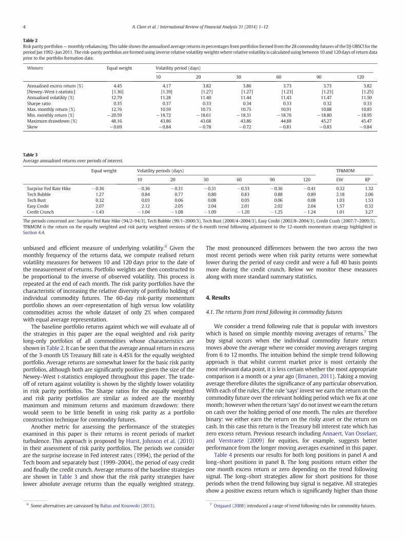
Table 2Risk parity portfolios—monthly rebalancing. This table shows the annualised average returns inpercentages fromportfolios formed from the28 commodity futures of theDJ-UBSCI for theperiod Jan 1992–Jun 2011. The risk-parity portfolios are formedusing inverse relative volatility weightswhere relative volatility is calculated using between 10 and 120days of return dataprior to the portfolio formation date.
Winners Equal weight Volatility period (days)
10 20 30 60 90 120
Annualised excess return (%) 4.45 4.17 3.82 3.86 3.73 3.73 3.82[Newey–West t-statistic] [1.36] [1.39] [1.27] [1.27] [1.23] [1.23] [1.25]Annualised volatility (%) 12.79 11.28 11.40 11.44 11.43 11.47 11.50Sharpe ratio 0.35 0.37 0.33 0.34 0.33 0.32 0.33Max. monthly return (%) 12.76 10.59 10.75 10.75 10.91 10.88 10.85Min. monthly return (%) −20.59 −18.72 −18.61 −18.31 −18.76 −18.80 −18.95Maximum drawdown (%) 48.16 43.86 43.68 43.86 44.88 45.27 45.47Skew −0.69 −0.84 −0.78 −0.72 −0.81 −0.83 −0.84
Table 3Average annualised returns over periods of interest.
Equal weight Volatility periods (days) TF&MOM
10 20 30 60 90 120 EW RP
Surprise Fed Rate Hike −0.36 −0.36 −0.31 −0.31 −0.33 −0.36 −0.41 0.32 1.32Tech Bubble 1.27 0.84 0.77 0.80 0.83 0.88 0.89 2.18 2.06Tech Bust 0.32 0.03 0.06 0.08 0.05 0.06 0.08 1.03 1.53Easy Credit 2.07 2.12 2.05 2.04 2.01 2.02 2.04 1.57 0.32Credit Crunch −1.43 −1.04 −1.08 −1.09 −1.20 −1.25 −1.24 1.01 3.27
The periods concerned are: Surprise Fed Rate Hike (94/2–94/3), Tech Bubble (99/1–2000/3), Tech Bust (2000/4–2004/3), Easy Credit (2002/8–2004/3), Credit Crash (2007/7–2009/3).TF&MOM is the return on the equally weighted and risk parity weighted versions of the 6-month trend following adjustment to the 12-month momentum strategy highlighted inSection 4.4.
4 A. Clare et al. / International Review of Financial Analysis 31 (2014) 1–12
unbiased and efficient measure of underlying volatility.6 Given themonthly frequency of the returns data, we compute realised returnvolatility measures for between 10 and 120 days prior to the date ofthe measurement of returns. Portfolio weights are then constructed tobe proportional to the inverse of observed volatility. This process isrepeated at the end of each month. The risk parity portfolios have thecharacteristic of increasing the relative diversity of portfolio holding ofindividual commodity futures. The 60-day risk-parity momentumportfolio shows an over-representation of high versus low volatilitycommodities across the whole dataset of only 2% when comparedwith equal average representation.
The baseline portfolio returns against which we will evaluate all ofthe strategies in this paper are the equal weighted and risk paritylong-only portfolios of all commodities whose characteristics areshown in Table 2. It can be seen that the average annual return in excessof the 3-month US Treasury Bill rate is 4.45% for the equally weightedportfolio. Average returns are somewhat lower for the basic risk parityportfolios, although both are significantly positive given the size of theNewey–West t-statistics employed throughout this paper. The trade-off of return against volatility is shown by the slightly lower volatilityin risk parity portfolios. The Sharpe ratios for the equally weightedand risk parity portfolios are similar as indeed are the monthlymaximum and minimum returns and maximum drawdown: therewould seem to be little benefit in using risk parity as a portfolioconstruction technique for commodity futures.
Another metric for assessing the performance of the strategiesexamined in this paper is their returns in recent periods of marketturbulence. This approach is proposed by Hurst, Johnson et al. (2010)in their assessment of risk parity portfolios. The periods we considerare the surprise increase in Fed interest rates (1994), the period of theTech boom and separately bust (1999–2004), the period of easy creditand finally the credit crunch. Average returns of the baseline strategiesare shown in Table 3 and show that the risk parity strategies havelower absolute average returns than the equally weighted strategy.
6 Some alternatives are canvassed by Baltas and Kosowski (2013).
The most pronounced differences between the two across the twomost recent periods were when risk parity returns were somewhatlower during the period of easy credit and were a full 40 basis pointsmore during the credit crunch. Below we monitor these measuresalong with more standard summary statistics.
4. Results
4.1. The returns from trend following in commodity futures
We consider a trend following rule that is popular with investorswhich is based on simple monthly moving averages of returns.7 Thebuy signal occurs when the individual commodity future returnmoves above the average where we consider moving averages rangingfrom 6 to 12months. The intuition behind the simple trend followingapproach is that whilst current market price is most certainly themost relevant data point, it is less certain whether themost appropriatecomparison is a month or a year ago (Ilmanen, 2011). Taking a movingaverage therefore dilutes the significance of any particular observation.With each of the rules, if the rule ‘says’ invest we earn the return on thecommodity future over the relevant holding period whichwe fix at onemonth; howeverwhen the return ‘says’do not investwe earn the returnon cash over the holding period of one month. The rules are thereforebinary: we either earn the return on the risky asset or the return oncash. In this case this return is the Treasury bill interest rate which haszero excess return. Previous research including Annaert, Van Osselaer,and Verstraete (2009) for equities, for example, suggests betterperformance from the longer moving averages examined in this paper.
Table 4 presents our results for both long positions in panel A andlong–short positions in panel B. The long positions return either theone month excess return or zero depending on the trend followingsignal. The long–short strategies allow for short positions for thoseperiods when the trend following buy signal is negative. All strategiesshow a positive excess return which is significantly higher than those
7 Ostgaard (2008) introduced a range of trend following rules for commodity futures.
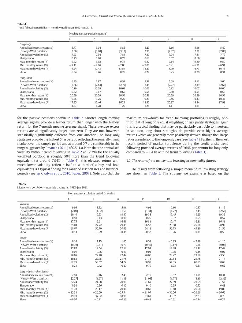
Table 4Trend following portfolios — monthly trading Jan 1992–Jun 2011.
Moving average period (months)
6 7 8 9 10 11 12
Long-onlyAnnualised excess return (%) 5.77 6.04 5.86 5.29 5.16 5.16 5.40[Newey–West t-statistic] [3.06] [3.20] [3.13] [2.90] [2.87] [2.81] [2.88]Annualised volatility (%) 7.93 7.94 7.84 7.80 7.74 7.81 7.79Sharpe ratio 0.73 0.76 0.75 0.68 0.67 0.66 0.69Max. monthly return (%) 9.92 9.92 9.37 9.37 9.14 9.80 9.80Min. monthly return (%) −7.11 −7.06 −7.06 −7.06 −6.91 −6.91 −6.91Maximum drawdown (%) 14.24 12.43 13.57 15.20 15.99 16.73 16.76Skew 0.34 0.46 0.29 0.27 0.25 0.29 0.31
Long–shortAnnualised excess return (%) 6.35 6.87 6.52 5.38 5.09 5.11 5.60[Newey–West t-statistic] [2.66] [2.84] [2.77] [2.38] [2.27] [2.39] [2.63]Annualised volatility (%) 10.19 10.29 10.04 10.03 10.12 10.07 10.00Sharpe ratio 0.62 0.67 0.65 0.54 0.50 0.51 0.56Max. monthly return (%) 20.59 20.59 20.59 20.59 20.59 20.59 20.59Min. monthly return (%) −9.25 −9.25 −9.25 −9.25 −9.46 −10.33 −10.33Maximum drawdown (%) 17.35 17.46 16.24 18.80 20.97 18.84 17.98Skew 1.27 1.28 1.29 1.28 1.11 1.11 1.10
5A. Clare et al. / International Review of Financial Analysis 31 (2014) 1–12
for the passive positions shown in Table 2. Shorter length movingaverage signals provide a higher return than longer with the highestreturn for the 7-month moving average signal. These average excessreturns are all significantly larger than zero. They are not, however,statistically significantly different from one another. The long onlystrategies provide thehighest Sharpe ratio reflecting the generally risingmarket over the sample period and at around 0.7 are comfortably in therange suggested by Ilmanen (2011) of 0.5–1.0. Note that the annualisedvolatility without trend following in Table 2 at 12.79% for the equallyweighted portfolio is roughly 50% more than the trend followingequivalent (at around 7.94% in Table 4): this elevated return withmuch lower volatility (often a half to a third of a buy and holdequivalent) is a typical finding for a range of asset classes and historicalperiods (see ap Gwilym et al., 2010; Faber, 2007). Note also that the
Table 5Momentum portfolios — monthly trading Jan 1992–Jun 2011.
Momentum calculation period (months)
6 7 8
WinnersAnnualised excess return (%) 9.95 8.52 5.91[Newey–West t-statistic] [2.09] [1.92] [1.50Annualised volatility (%) 20.10 19.93 19.87Sharpe ratio 0.50 0.43 0.30Max. monthly return (%) 17.75 16.61 16.61Min. monthly return (%) −25.04 −27.72 −29.45Maximum drawdown (%) 48.67 50.70 50.63Skew −0.14 −0.29 −0.44
LosersAnnualised excess return (%) 0.16 1.13 1.65[Newey–West t-statistic] [0.39] [0.61] [0.73Annualised volatility (%) 17.87 17.54 17.18Sharpe ratio 0.01 0.06 0.10Max. monthly return (%) 20.05 22.40 22.42Min. monthly return (%) −19.83 −22.75 −21.78Maximum drawdown (%) 62.29 58.57 54.24Skew 0.21 0.42 0.47
Long winners–short losersAnnualised excess return (%) 7.58 5.46 2.49[Newey–West t-statistic] [2.27] [1.97] [1.13Annualised volatility (%) 22.24 21.08 20.98Sharpe ratio 0.34 0.26 0.12Max. monthly return (%) 21.49 20.17 20.40Min. monthly return (%) −22.38 −26.50 −25.54Maximum drawdown (%) 49.49 37.02 48.98Skew −0.07 −0.21 −0.13
maximum drawdown for trend following portfolios is roughly one-third that of long only equal weighting or risk parity strategies: againthis is a typical finding that may be particularly desirable to investors.In addition, long–short strategies do provide even higher averagereturns which are generally more positively skewed, though the Sharperatios are inferior to the long-only case (see Table 4). Further in themostrecent period of market turbulence during the credit crisis, trendfollowing provided average returns of 0.64% per annum for long only,compared to −1.43% with no trend following (Table 3).
4.2. The returns from momentum investing in commodity futures
The results from following a simple momentum investing strategyare shown in Table 5. The strategy we examine is based on the
9 10 11 12
4.93 7.10 10.67 11.12] [1.34] [1.77] [2.45] [2.53]
19.38 19.45 19.25 19.360.25 0.37 0.55 0.57
16.81 17.47 16.81 16.81−26.52 −25.88 −25.88 −28.92
54.11 52.73 49.80 51.56−0.32 −0.26 −0.31 −0.56
0.58 −0.83 −2.49 −1.16] [0.49] [0.17] [0.26] [0.08]
17.91 17.88 17.12 17.420.03 −0.05 −0.15 −0.07
26.60 28.22 23.56 23.56−21.78 −20.64 −21.78 −21.14
50.98 57.35 69.55 60.680.79 1.03 0.61 0.62
2.19 5.57 11.31 10.31] [1.08] [1.77] [3.10] [2.82]
21.67 22.59 21.69 21.530.10 0.25 0.52 0.48
20.60 19.48 20.60 19.89−31.07 −32.56 −26.66 −26.66
53.63 46.37 32.23 38.76−0.48 −0.61 −0.24 −0.27
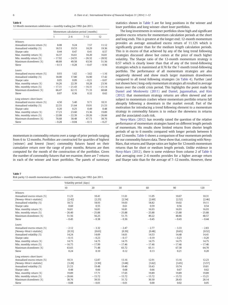
Table 612-Month momentum subdivision — monthly trading Jan 1992–Jun 2011.
Momentum calculation period (months)
1 2–6 7–12 12
WinnersAnnualised excess return (%) 8.08 9.24 7.57 11.12Annualised volatility (%) 18.53 19.53 18.29 19.36Sharpe ratio 0.44 0.47 0.41 0.57Max. monthly return (%) 16.37 16.61 18.20 16.81Min. monthly return (%) −17.92 −24.55 −26.32 −28.92Maximum drawdown (%) 48.88 49.58 63.56 51.56Skew −0.13 −0.28 −0.47 −0.56
LosersAnnualised excess return (%) 0.93 1.62 −3.62 −1.16Annualised volatility (%) 18.00 17.80 16.90 17.42Sharpe ratio 0.05 0.09 −0.21 −0.07Max. monthly return (%) 16.26 22.39 18.28 23.56Min. monthly return (%) −17.31 −21.43 −16.31 −21.14Maximum drawdown (%) 66.47 62.15 71.33 60.68Skew 0.07 0.36 0.32 0.62
Long winners–short losersAnnualised excess return (%) 4.50 5.40 9.71 10.31Annualised volatility (%) 22.55 21.64 19.91 21.53Sharpe ratio 0.20 0.25 0.49 0.48Max. monthly return (%) 17.23 23.60 15.36 19.89Min. monthly return (%) −22.08 −22.39 −20.26 −26.66Maximum drawdown (%) 76.68 38.48 47.73 38.76Skew −0.28 −0.04 −0.11 −0.27
6 A. Clare et al. / International Review of Financial Analysis 31 (2014) 1–12
momentum in commodity returns over a range of prior periods rangingfrom 6 to 12months. Portfolios are constructed for quartiles of highest(winner) and lowest (loser) commodity futures based on theircumulative return over the range of prior months. Returns are thencomputed for the month of the construction of the portfolios. Giventhe number of commodity futures that we examine, there are 7 returnsin each of the winner and loser portfolios. The panels of summary
Table 7Risk parity 12-month momentum portfolios — monthly trading Jan 1992–Jun 2011.
Volatility period (days)
10 20
WinnersAnnualised excess return (%) 11.23 10.41[Newey–West t-statistic] [2.42] [2.25]Annualised volatility (%) 18.72 18.93Sharpe ratio 0.60 0.55Max. monthly return (%) 16.81 16.81Min. monthly return (%) −26.40 −25.88Maximum drawdown (%) 51.56 56.25Skew −0.45 −0.38
LosersAnnualised excess return (%) −2.12 −3.32[Newey–West t-statistic] [0.33] [0.63]Annualised volatility (%) 14.24 14.69Sharpe ratio −0.15 −0.23Max. monthly return (%) 14.75 14.75Min. monthly return (%) −16.75 −17.99Maximum drawdown (%) 63.65 71.48Skew 0.24 0.10
Long winners–short losersAnnualised excess return (%) 10.31 12.87[Newey–West t-statistic] [3.28] [3.50]Annualised volatility (%) 21.53 19.48Sharpe ratio 0.48 0.66Max. monthly return (%) 19.89 17.71Min. monthly return (%) −26.66 −15.72Maximum drawdown (%) 38.76 39.55Skew −0.08 −0.01
statistics shown in Table 5 are for long positions in the winner andloser portfolios and long winner–short loser portfolios.
The long investments inwinner portfolios show high and significantpositive excess returns for momentum calculation periods at the shortand long ends. This is greatest at the longer end; 12-month momentumprovides an average annualised excess return of 11.12% which issignificantly greater than for the medium length calculation periods.This is in excess of that achieved by any of the long trend followingstrategies discussed above but comes at the price of much highervolatility. The Sharpe ratio of the 12-month momentum strategy is0.57 which is clearly lower than that of any of the trend-followingstrategies which is maximised at 0.76 for the 7-month trend-followingportfolio. The performance of all momentum strategies are alsonegatively skewed and show much larger maximum drawdownscompared to all trend following strategies (in Table 4). Further (andnot shownhere) long-onlymomentum strategies all resulted in averagelosses over the credit crisis period. This highlights the point made byDaniel and Moskowitz (2011) and Daniel, Jagannathan, and Kim(2012) that momentum strategy returns are often skewed and aresubject to momentum crashes where momentum portfolio returns fallabruptly following a downturn in the market overall. Part of themotivation for introducing a trend following element to a momentumstrategy in commodity futures is to reduce the skewness in returnsand the associated crash risk.
Novy-Marx (2012) has recently raised the question of the relativeperformance of momentum strategies based on different length periodsof momentum. His results show limited returns from shorter lengthperiods of up to 6 months compared with longer periods between 6and 12months. Table 6 shows a comparison of four momentum periodsfor our commodity futures data. These show that, contrastingwithNovy-Marx, that returns and Sharpe ratios are higher for 12monthmomentumreturns than for short or medium length periods. Unlike evidence inNovy-Marx (2012), there is some evidence from column 2 of Table 6that averaging over 2–6 months provides for a higher average returnand Sharpe ratio than for the average of 7–12months. However, these
30 60 90 120
11.61 11.05 10.67 10.31[2.54] [2.60] [2.52] [2.46]19.03 18.82 19.02 19.110.61 0.59 0.56 0.54
16.81 16.93 16.93 16.93−25.88 −25.88 −25.88 −25.88
51.75 49.22 48.86 48.57−0.36 −0.45 −0.43 −0.44
−2.47 −2.77 −3.33 −2.83[0.39] [0.48] [0.65] [0.52]14.61 14.53 14.48 14.41−0.17 −0.19 −0.23 −0.2014.75 14.75 14.75 14.75
−17.46 −17.46 −17.46 −17.4665.72 65.11 67.30 64.700.12 0.13 0.21 0.20
13.16 12.91 13.16 12.23[3.68] [3.62] [3.65] [3.57]19.40 19.43 19.74 19.810.68 0.66 0.67 0.62
17.65 19.89 19.89 19.89−15.72 −15.72 −15.72 −15.21
31.72 30.30 28.43 28.14−0.01 0.00 0.02 0.05

7A. Clare et al. / International Review of Financial Analysis 31 (2014) 1–12
are both dominated by the 12 month period. The discontinuity inperformance raises questions about the applicability of popularbehavioural and rational explanations of the effectiveness ofmomentumstrategies.
4.3. Risk parity trend following and momentum portfolios
The portfolio returns shown in Tables 4 and 5 for trend following andmomentumportfolios separately are for the standard equally-weightedcases. Next, we evaluate the contribution that risk-parity weightingmight make to these strategies. Table 7 provides results for the highestreturn, 12-month momentum strategy for a range of volatilitymeasurement periods and is directly comparable to the last column inTable 5. As with the simple raw returns reported above in Table 2, theimpact of risk-parity weighting is to increase the presence of lowervolatility commodities in portfolios. Thus amongst winner portfolios,returns are slightly less volatile and have a somewhat lower maximumdrawdown as well as being less negatively skewed than in the equally-weighted case. Average returns for winners are higher for somevolatility periods. The performance of loser portfolios is much worseunder risk-parity weighting although this is not significantly differentfrom zero given the size of the t-statistics. Consequently, averagereturns and Sharpe ratios for winner-loser portfolios are much higherin this case. For a 30-day volatilitymeasurement period, average returnsare some 13.16% with a Sharpe ratio of 0.68 compared to, say, 10.31%and 0.48 for the long–short equally weighted portfolio in Table 5
Table 8Risk parity trend following portfolios — monthly trading Jan 1992–Jun 2011.
Volatility period (days)
7-month moving average signal 10 20 30
Long-onlyAnnualised excess return (%) 5.01 5.10 5.2[Newey–West t-statistic] [2.97] [2.94] [2.9Annualised volatility (%) 7.08 7.16 7.1Sharpe ratio 0.71 0.71 0.7Max. monthly return (%) 8.62 9.25 9.4Min. monthly return (%) −7.30 −6.98 −6.7Maximum drawdown (%) 13.30 13.06 12.7Skew 0.12 0.22 0.3
Long–shortAnnualised excess return (%) 5.29 5.84 6.0[Newey–West t-statistic] [2.64] [2.81] [2.8Annualised volatility (%) 8.91 8.95 8.9Sharpe ratio 0.59 0.65 0.6Max. monthly return (%) 18.72 18.61 18.3Min. monthly return (%) −7.35 −7.14 −6.8Maximum drawdown (%) 15.31 14.45 14.0Skew 1.46 1.43 1.3
12-month moving average signal
Long-onlyAnnualised excess return (%) 5.05 4.99 5.0[Newey–West t-statistic] [2.83] [2.75] [2.7Annualised volatility (%) 7.05 7.10 7.1Sharpe ratio 0.72 0.70 0.7Max. monthly return (%) 8.80 9.42 9.5Min. monthly return (%) −7.03 −6.68 −6.6Maximum drawdown (%) 15.76 15.52 15.5Skew 0.24 0.30 0.3
Long–shortAnnualised excess return (%) 5.37 5.60 5.7[Newey–West t-statistic] [2.77] [2.81] [2.8Annualised volatility (%) 8.81 8.85 8.8Sharpe ratio 0.61 0.63 0.6Max. monthly return (%) 18.72 18.61 18.3Min. monthly return (%) −8.09 −8.03 −8.1Maximum drawdown (%) 15.79 15.84 16.1Skew 1.38 1.37 1.2
(12monthmomentum calculation period). Overall the results of addingthe risk parity overlay to momentum investing have limited impact onthe results but do lead to some overall improvement, especially withregard to maximum drawdowns.
What if we overlay trend following on the simple returns and applyrisk-parity weighting? The results are shown in Table 8, where 7- and12-month moving average-based strategies are reported, and may becompared with the equally weighted version in Table 4 which has notrend following. These show, as with the results for momentumstrategies, that the biggest impact of risk-parity weighting is on loserportfolios and, consequently, on long winner–short loser portfolios.Average returns and Sharpe ratios are significantly higher for long–short portfolios for longer volatility calculation periods with the trendfollowing overlay. These should also be compared with the risk-parityportfolios in Table 2 which do not adjust for trend following, wheredrawdowns are at least 3 times as big and Sharpe ratios are only halfthe size of Table 8. These results show that risk-parity weighting canhave rather limited effects relative to equal weighting but that morepredictable and substantial effects come from applying trend following.
Inker (2010) has raised a number of concerns with risk parityweighting in the context of strategies in equity and bond markets.These are mostly concerned with the use of leverage to extend theweight given to bonds in portfolios which we do not consider here.The remaining concern raised by Inker is that the attractiveness ofpreviously low volatility return assets such as bonds might beoverstated as they are subject to significant skewness risk. In our
60 90 120 180
2 5.35 5.40 5.51 5.515] [3.03] [3.03] [3.07] [3.05]7 7.13 7.20 7.22 7.243 0.75 0.75 0.76 0.761 9.73 9.62 9.67 9.769 −6.73 −6.72 −6.74 −6.758 12.65 12.69 12.74 12.773 0.37 0.33 0.35 0.36
3 6.41 6.52 6.64 6.525] [2.92] [2.93] [2.94] [2.86]4 8.96 9.00 9.04 9.107 0.72 0.72 0.73 0.721 18.76 18.80 18.95 19.065 −6.70 −6.78 −6.73 −6.843 12.23 12.01 12.69 12.969 1.55 1.51 1.55 1.56
9 5.18 5.19 5.29 5.268] [2.87] [2.86] [2.90] [2.88]3 7.07 7.11 7.14 7.171 0.73 0.73 0.74 0.736 9.74 9.62 9.69 9.718 −6.44 −6.54 −6.53 −6.434 15.34 15.41 15.50 15.677 0.39 0.35 0.37 0.38
7 6.08 6.09 6.20 6.028] [3.03] [3.01] [3.05] [2.98]9 8.87 8.89 8.92 8.965 0.69 0.68 0.69 0.671 18.76 18.80 18.95 19.063 −7.96 −7.72 −7.66 −7.735 14.65 14.69 14.18 14.037 1.43 1.42 1.46 1.48
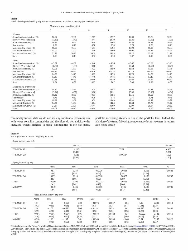
Table 9Trend following 60-day risk parity 12-month momentum portfolios — monthly Jan 1992–Jun 2011.
Moving average period (months)
6 7 8 9 10 11 12
WinnersAnnualised excess return (%) 12.77 12.90 12.87 12.37 12.09 11.79 12.43[Newey–West t-statistic] [3.39] [3.49] [3.41] [3.30] [3.26] [3.10] [3.23]Annualised volatility (%) 16.17 16.41 16.54 16.64 16.56 16.83 16.91Sharpe ratio 0.79 0.79 0.78 0.74 0.73 0.70 0.73Max. monthly return (%) 16.93 16.93 16.93 16.93 16.93 16.93 16.93Min. monthly return (%) −13.00 −13.00 −13.00 −13.00 −13.00 −14.26 −14.26Maximum drawdown (%) 31.43 30.73 30.19 28.95 28.22 32.18 31.79Skew 0.06 0.14 0.12 0.10 0.07 0.00 0.01
LosersAnnualised excess return (%) −3.07 −4.02 −3.46 −3.26 −3.07 −3.23 −3.40[Newey–West t-statistic] [0.72] [1.04] [0.80] [0.71] [0.64] [0.69] [0.74]Annualised volatility (%) 12.93 12.97 13.22 13.50 13.62 13.65 13.78Sharpe ratio −0.24 −0.31 −0.26 −0.24 −0.23 −0.24 −0.25Max. monthly return (%) 14.75 14.75 14.75 14.75 14.75 14.75 14.75Min. monthly return (%) −17.46 −17.46 −17.46 −17.46 −17.46 −17.46 −17.46Maximum drawdown (%) 62.18 66.65 66.46 66.79 64.66 64.64 66.52Skew 0.04 0.07 0.07 0.07 0.05 0.05 0.08
Long winners–short losersAnnualised excess return (%) 14.70 15.94 15.28 14.48 13.92 13.88 14.69[Newey–West t-statistic] [3.84] [4.07] [3.98] [3.91] [3.86] [3.86] [4.04]Annualised volatility (%) 19.33 19.53 19.33 19.54 19.56 19.53 19.65Sharpe ratio 0.76 0.82 0.79 0.74 0.71 0.71 0.75Max. monthly return (%) 19.59 19.59 19.59 19.89 19.89 19.89 19.89Min. monthly return (%) −14.84 −14.84 −14.84 −14.84 −14.84 −15.72 −15.72Maximum drawdown (%) 31.87 32.01 31.44 31.00 30.07 30.17 30.83Skew −0.08 −0.10 −0.09 −0.06 −0.07 0.00 −0.02
8 A. Clare et al. / International Review of Financial Analysis 31 (2014) 1–12
commodity futures data we do not see any substantial skewness riskwith lower volatility commodities and therefore do not anticipate theincreased weight attached to these commodities in the risk parity
Table 10Risk adjustment of returns: long only portfolios.
Simple average–long only
Average
TF & MOM RP 1.126[3.49]
TF & MOM EW 1.125[3.42]
Equity factors–long only
Alpha MKT S
TF & MOM RP 0.877 0.233 −[2.80] [3.24]
TF & MOM EW 0.873 0.218 −[2.83] [3.05]
TF RP 0.350 0.104[2.41] [2.61]
MOM VW 0.649 0.436[1.64] [3.54]
Hedge fund risk factors–long only
Alpha SBD SFX SCOM EMF
TF & MOM RP 1.14 −1.59 −0.539 8.89 −0.0[3.42] [0.89] [0.38] [3.63] [0.7
TF & MOM EW 1.16 −1.02 −0.985 8.04 −0.1[3.39] [0.60] [0.71] [3.81] [0.9
TF RP 0.464 −0.564 −0.304 4.05 −0.0[3.08] [0.69] [0.50] [3.53] [1.3
MOM RP 0.910 −1.19 −1.17 6.61 −0.0[2.36] [0.46] [0.63] [2.23] [0.1
The risk factors are; the Fama–French four US equitymarket factors, MKT, SMB, HML and UMDCurrency (SFX) and Commodity Trend (SCOM) lookback straddle returns; EquityMarket FactorEmergingMarket Risk Factor (EMRF). Portfolios are either equal-weight (EW) or risk-parity weMOM).
portfolio increasing skewness risk at the portfolio level. Indeed theaddition of the trend following component reduces skewness in returnsas is noted above.
Average
TF RP 0.463[3.03]
MOMRP 1.026[2.60]
MB HML UMD R2
0.0036 0.0823 0.158 0.0844[0.04] [0.92] [3.01]0.0018 0.0877 0.173 0.0797[0.02] [0.99] [3.19]0.00732 0.0546 0.0562 0.0420[0.19] [1.44] [2.01]0.0075 0.136 0.146 0.0705[0.08] [1.47] [2.42]
SSF BMF CSF EMRF R2
974 0.0557 1.64 −1.28 0.200 0.03125] [0.52] [1.11] [1.41] [2.25]19 0.0731 1.42 −0.773 0.201 0.03020] [0.69] [0.90] [0.73] [2.29]878 −0.0442 1.21 0.0222 0.142 0.03111] [1.13] [1.69] [0.05] [3.36]260 0.0938 −1.46 −5.31 0.257 0.03229] [0.86] [0.72] [2.19] [2.57]
and, secondly the eight hedge fund factors of Fung andHsieh (2001): the PTFS Bond (SBD),(EMF), Size Spread Factor (SSF), BondMarket Factor (BMF), Credit Spread Factor (CSF) andighted (RP) for trend following (TF),momentum (MOM) or a combination of the two (TF &
8 These results are available from the authors.
Table 11Risk adjustment: long–short portfolios.
Simple average–long–short
Average Average
TF & MOM RP 1.398 TF RP 0.565[4.07] [2.92]
TF & MOM EW 1.272 MOMRP 1.172[3.41] [3.62]
Equity factors–long–short
Alpha MKT SMB HML UMD R2
TF & MOM RP 1.238 −0.0064 −0.0014 0.042 0.263 0.0780[3.46] [0.06] [0.02] [0.36] [3.75]
TF & MOM EW 1.11 −0.0948 0.0512 0.0998 0.296 0.116[2.90] [0.85] [0.52] [0.70] [4.20]
TF RP 0.601 −0.122 −0.0307 −0.0299 0.0847 0.0644[2.65] [1.25] [1.04] [0.46] [3.05]
MOM RP 0.930 0.142 0.0312 0.0866 0.225 0.0576[2.85] [1.71] [0.37] [0.77] [3.05]
Hedge fund risk factors–long–short
Alpha SBD SFX SCOM EMF SSF BMF CSF EMRF R2
TF & MOM RP 1.49 −0.753 −0.310 7.10 −0.141 0.124 1.53 0.761 0.0246 0.0215[4.00] [0.36] [0.16] [2.07] [0.92] [0.86] [0.78] [0.41] [0.24]
TF & MOM EW 1.44 −2.31 −1.35 7.17 −0.139 0.191 1.34 0.211 −0.0642 0.0296[3.64] [1.13] [0.66] [2.24] [0.91] [1.25] [0.64] [1.36] [0.58]
TF RP 0.687 −0.367 0.0528 4.15 −0.146 −0.0546 2.31 2.57 0.0301 0.0226[3.33] [0.33] [0.06] [2.43] [2.03] [1.25] [1.92] [1.84] [0.70]
MOM RP 1.15 0.563 −0.928 3.37 −0.0496 0.221 −2.15 −3.50 0.0233 0.0312[3.22] [0.23] [0.48] [0.96] [0.33] [1.60] [1.10] [2.20] [0.23]
The risk factors are: the Fama–French four US equitymarket factors, MKT, SMB, HML and UMD and, secondly the eight hedge fund factors of Fung andHsieh (2001): the PTFS Bond (SBD),Currency (SFX) and Commodity Trend (SCOM) lookback straddle returns; EquityMarket Factor (EMF), Size Spread Factor (SSF), BondMarket Factor (BMF), Credit Spread Factor (CSF) andEmergingMarket Risk Factor (EMRF). Portfolios are either equal-weight (EW) or risk-parity weighted (RP) for trend following (TF),momentum (MOM) or a combination of the two (TF &MOM).
9A. Clare et al. / International Review of Financial Analysis 31 (2014) 1–12
4.4. The performance of combined trend following andmomentumportfolios
Finally, we examine whether combining the two strategies couldprovide a set of portfolios which perform better than either of the twostrategies alone. Interest in combined strategies has arisen in the contextof designing strategies in a variety of markets outside of commodityfutures, see Antonacci (2012), for example. Our results shown in Table 9provide the summary evidence for a set of combined strategies; those ofbetween 6 and 12-month trend following and 12-month momentumrisk-parity portfolios based on a 60-day volatility calculation. For acommodity tonowbe in thewinner portfolio itmust be in the topquartileof assets based on the momentum calculation and also have a positivetrend according to the trend following rule. Losers must be in the bottomquintile of the momentum rankings and have a negative trend.Considering winner portfolios, the average excess returns from thesestrategies exceed those from any of the winner strategies examinedthus far. Compared with momentum-only returns in Table 5 with, say a12 month momentum period, the 7 month moving average trendfollowing return at 12.90% is over 1.85% higher with a standard error of0.27%. As a result of the impact of the lower volatility of trend followingstrategies, these higher returns are achieved at lower levels of volatilitythan in the case of momentum-only strategies and so have a higherSharpe ratio than any of the previous strategies. There is no evidence ofany skewness in these returns and they are also subject to lowermaximum drawdown than previous strategies. Loser portfolios providea consistently small negative and more volatile set of returns which arealso not skewed. Winner–loser portfolios thus provide the highest set ofreturns for all trend-following moving average calculation periods andgenerate the highest average excess return of 15.94% and a Sharpe ratioof 0.82. (Table 9)These results show that amongst all momentumstrategies, the introduction of trend following leads to reduced variabilityand a positive impact on skewness. If the risk-parity results in Table 9 arecompared with those from equally weighted portfolios with similar
momentum and moving average parameters, it can be shown that riskparity leads to slightly higher average returns at a lower level ofvolatility.8 This is consistent with the original promoters of risk-parityportfolios and the evaluations of broader asset classes such as Asnesset al. (2013), for example. Finally, examining the periods of marketturbulence, the final column of Table 3 shows that both equally weightedand risk parity returns from the combined 6-month trend following and12-month momentum strategy provide positive returns over all of theseperiods and, in particular, the most recent credit crisis period where thewinner–loser strategy delivered in excess of 3% pa.
In this section we have shown that whilst a momentum strategy candeliver high returns, this is associated with high negative skewness andmaximum drawdown. This is true of equally and risk parity weightedversions of the strategy and for long-only winners portfolios and long–short, winners–losers strategies. Trend following in itself provides amore modest but significantly higher return than passive strategies buthigher Sharpe ratios reflecting reduced volatility. The addition of trendfollowing to a momentum strategy reduces the downside risk of themomentum approach without sacrificing returns. The reduced negativeskewness is also reflected in reduced maximum drawdown. Whetherthe significant enhanced average returns from these strategies iscompensation for exposure to important risk factors is our next concern.
5. Understanding the profitability of strategy returns
5.1. Risk adjusted returns
The properties of returns presented thus far refer to unconditionalreturns from trend following and momentum strategies. In this sectionwe examine whether these excess returns are explained by widely
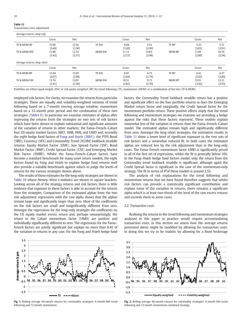
Table 12Transactions costs adjustment.
Average returns–long only
Gross Net Gross Net Gross Net
TF & MOM RP 12.90 12.62 TF EW 6.04 5.91 TF RP 5.35 5.31[3.49] [3.38] [3.20] [2.99] [3.03] [2.91]
TF & MOM EW 12.86 12.52 MOM EW 11.12 10.83 MOM RP 11.05 10.76[3.42] [3.37] [2.53] [2.48] [2.60] [2.54]
Average returns–long–short
Gross Net Gross Net Gross Net
TF & MOM RP 15.94 15.65 TF EW 6.87 6.75 TF RP 6.41 6.37[4.07] [3.99] [2.84] [2.79] [2.92] [2.86]
TF & MOM EW 13.76 13.01 MOM EW 10.31 9.75 MOM RP 12.91 12.21[3.41] [3.38] [2.82] [2.70] [3.62] [3.55]
Portfolios are either equal-weight (EW) or risk-parity weighted (RP) for trend following (TF), momentum (MOM) or a combination of the two (TF & MOM).
10 A. Clare et al. / International Review of Financial Analysis 31 (2014) 1–12
employed risk factors. For clarity,we examine the returns fromparticularstrategies. These are equally and volatility-weighted versions of trendfollowing based on a 7-month moving average window, momentumbased on a 12-month prior period and the combination of these twostrategies (Tables 9). In particular we examine estimates of alphas afterregressing the returns from the strategies on two sets of risk factorswhich have been shown to explain substantial and significant amountsof the variation of returns in other markets; the Fama–French–Cahartfour US equity market factors, MKT, SMB, HML and UMD and, secondlythe eight hedge fund factors of Fung and Hsieh (2001): the PTFS Bond(SBD), Currency (SFX) and Commodity Trend (SCOM) lookback straddlereturns; Equity Market Factor (EMF), Size Spread Factor (SSF), BondMarket Factor (BMF), Credit Spread Factor (CSF) and Emerging MarketRisk Factor (EMRF). Whilst the Fama–French–Cahart factors havebecome a standard benchmark for many asset return models, the eightfactors found by Fung and Hsieh to explain hedge fund returns wellalso provide a suitable benchmark against which to judge the levels ofreturns for the various strategies shown above.
The results of these estimates for the long-only strategies are shown inTable 10 where Newey–West t-statistics are shown in square brackets.Looking across all of the strategy returns and risk factors, there is littleevidence that exposure to these factors is able to account for the returnsfrom the strategies. Comparison of the estimated alphas from the tworisk adjustment regressions with the raw alpha shows that the alphasremain large and significantly larger than zero. Most of the coefficientson the risk factors are small and insignificantly different from zero.Amongst the regressions for the long-only strategies the coefficients onthe US equity market excess return and, perhaps unsurprisingly, thereturn to the Cahart momentum factor (UMD) are positive andindividually significantly different to zero. The regressions for the Fama–French factors are jointly significant but explain no more than 8.4% ofthe variation in returns in any case. For the Fung and Hsieh hedge fund
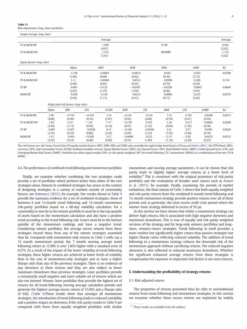
Fig. 1. Rolling average 36-month returns for commodity strategies: 6 month MA trendfollowing and 12month momentum.
factors, the Commodity Trend lookback straddle return has a positiveand significant effect on the four portfolio returns as does the EmergingMarket return factor and marginally, the Credit Spread factor for themomentum portfolio return. These positive effects imply that the trendfollowing and momentum strategies we examine are providing a hedgeagainst the risks that these factors represent. These models explainsomewhat less of the variation in returns than the Fama–French–Cahartmodel. The estimated alphas remain high and significantly differentfrom zero. Amongst the long–short strategies, the estimation results inTable 11 show a lower level of significant exposure to the two sets ofrisk factors and a somewhat reduced fit. In both cases the estimatedalphas are reduced less by the risk adjustment than in the long-onlycases. The Fama–French momentum factor UMD is significantly pricedin all of the first set of regressions, whilst the fit is generally below 10%.In the Fung–Hsieh hedge fund factors model, only the return from theCommodity trend lookback straddle is significant, although again theCredit Spread factor is significant in the case of the momentum-onlystrategy. The fit in terms of R2of these models is around 2.5%.
The analysis of risk explanations for the trend following andmomentum returns that we have found therefore suggests that whilstrisk factors can provide a statistically significant contribution andexplain some of the variation in returns, there remains a significantalpha which is at least two-thirds of the level of the raw excess returnsand exceeds them in some cases.
5.2. Transaction costs
Realising the returns to the trend following andmomentum strategiesanalysed in this paper in practice would require accommodatingtransaction costs, in this section we assess how the average returnspresented above might be modified by allowing for transaction costs.In doing this we try to be realistic by allowing for a fixed brokerage
Fig. 2. Rolling average 36-month returns for commodity strategies: 6 month MA trendfollowing and 12month momentum combined strategy.

11A. Clare et al. / International Review of Financial Analysis 31 (2014) 1–12
commission as well as applying a bid-ask spread. The sum of these costsis then subtracted from gross returns as a percentage of average contractvalue, assuming one round-turn trade everymonth. Following Szakmaryet al. (2010) we set the fixed brokerage fee at $10 per contract and thebid-ask spread at one tick. Locke and Venkatesh (1997) and discussionwith market participants suggest that this is a representative level forthe bid-ask spread in commodity futures markets.9 In our calculations,for the range of commodities, the fixed cost element amounts tobetween 6 and 0.5 basis points, whilst the one tick, bid-ask spread isbetween 5.2 and 0.7 basis points. Having applied these costs, thedifferences between gross returns and returns net of transaction costsfor the selected strategy returns evaluated in Section 5.1 can be seen inTable 12. The differences in average returns are not large at no morethan 0.5% and well within one standard error of the gross returns. Theextent to which trading costs have reduced over time due toimprovements in the efficiency of trading technologies would makethe net returns we analyse underestimates of performance in morerecent parts of the sample period. Assessment of time variation in returnsshould take this into account.
5.3. Time-variation in the returns to investment strategies
The analysis presented thus far focusses on average returns andperformance in particular episodes. The stability over time ofmomentum and trend following returns is clearly of interest —
especially to those with shorter investment horizons. In Figs. 1 and 2we present average excess returns to a number of strategies calculatedover rollingwindows of 36months. All of these returns show significanttime variation. This is more apparent in the behaviour of momentumreturns (Fig. 1) where the highest returns can be seen in the 2008–9period having been lowest in the 2004–6 period. Trend followingreturns show lower time variation and remain at an enhanced levelfrom 2009 to the end of the sample. It can be seen from the figuresthat the addition of trend following to the momentum strategiesdominates the difference in returns (Fig. 2): it matters less whetherthe portfolios are equally or risk-weighted (compare the lines inFig. 2). This is of importance for those investors with shorter investmenthorizons.10 As noted above, it can be expected that the performance ofreturns net of transaction costs for all strategies could be enhanced byimprovements in trading technologies in the later part of the sampleperiod.
6. Conclusion
It is no surprise that momentum and trend following rules arepopular with professional and retail investors alike. They offer enhancedreturns over passive strategies and sometimes higher Sharpe ratios invarious markets. In this paper we have shown that this is true forcommodity futures. We have shown significant average excess returnsfor momentum strategies but these come at the price of substantialnegative skewness and maximum drawdown. Our results demonstratemomentum crash risk as proposed by Daniel and Moskowitz (2011).We also show significant average excess returns for a variety of trendfollowing strategies. These produce somewhat lower returns thanmomentum rules but with higher Sharpe ratios and without the largenegative skewness. The addition of trend following to a momentumstrategy is shown to provide both high returns and lower drawdownsand skewness. This is especially true of portfolios where weights are
9 We apply these averages as the index data examined in this paper does not includeactual contracts.10 The potential limits to arbitragewhen strategy returns are time varying is surveyed byDuffie (2010). Time variation in simple momentum returns from foreign exchangemomentum strategies is shown by Menkhoff, Sarno, Schmeling, and Schrimpf (2012),although they do not examine trend following returns.
measured by inverse volatility rather thanbeing equal, thus overcomingthe large differences in volatility of different commodities. This findingadds to the literature which tries to explain momentum returns.In our results, the contribution to momentum performance of thecharacteristics offered in this literature are captured by trend following.We show that the enhanced average excess return to the strategiesexamined is not mainly compensation for exposure to well-known riskfactors and remains once account is taken of transaction costs. Whethercrash risk is a good explanation formomentum returns, this seems not tobe the case for trend-following or the combined momentum and trendfollowing strategies that we examine. In futureworkwe intend to followup on this idea.
References
Andersen, T. G., & Bollerslev, T. (1998). Answering the sceptics: Yes, standardvolatility models do provide accurate forecasts. International Economic Review,39(4), 885–905.
Annaert, J., Van Osselaer, S., & Verstraete, B. (2009). Performance evaluation of portfolioinsurance using stochastic dominance criteria. Journal of Banking and Finance, 33,272–280.
Antonacci, G. (2012). Risk premia harvesting through momentum. : Portfolio ManagementAssociates.
ap Gwilym, O., Clare, A., Seaton, J., & Thomas, S. (2010). Price and momentum as robusttactical approaches to global equity investing. Journal of Investing, 19, 80–92.
Asness, C., Frazzini, A., & Pedersen, L. (2011). Leverage aversion and risk parity. AQRcapital management working paper.
Asness, C., Moskowitz, T., & Pedersen, L. (2013). Value and momentum everywhere.Journal of Finance, 68(3), 929–985.
Avramov, D., Chordia, T., Jostova, G., & Philipov, A. (2007). Momentum and credit rating.Journal of Finance, 62, 407–427.
Baltas, A., & Kosowski, R. (2013). “Momentum Strategies in Futures Markets andTrend-Following Funds”, Imperial College, London, mimeo.
Bandarchuk, P., & Hilscher, J. (2013). Sources of momentum profits: Evidence on theirrelevance of characteristics. Review of Finance, 17(2), 809–845.
Basak, S., & Palova, A. (2013). A model of financialization of commodities. LondonBusiness School, mimeo.
Dalio (2004). Engineering targeted returns and risks. Bridgewater associates working paper.Daniel, K., Jagannathan, R., & Kim, S. (2012). Tail risk inmomentum strategy returns.NBER
working paper 18169.Daniel, K., & Moskowitz, T. (2011). Momentum crashes. Columbia business school research
paper.Dow-Jones (2012). DJ-UBS CI: The Dow Jones-UBS commodity index handbook. New York:
Dow Jones Indexes.Duffie, D. (2010). Asset pricing dynamics with slow-moving capital. Journal of Finance, 65,
1237–1267.Erb, C., & Harvey, C. (2006). The tactical and strategic value of commodity futures.
Financial Analysts Journal, 62, 69–97.Faber, M. (2007). A quantitative approach to tactical asset allocation. Journal of Investing, 16,
69–79.Faber, M. (2010). Relative strength strategies for investing. Cambria investment management
working paper.Fung,W., & Hsieh, D. (2001). The risk in hedge fund strategies: Theory and evidence from
trend followers. Review of Financial Studies, 14(2), 313–341.Gorton, G., & Rouwenhorst, G. (2006). Facts and fantasies about commodity futures.
Financial Analysts Journal., 62, 47–68.Hamilton, J., & Wu, J. (2013). “Effects of index-fund investing on commodity futures
prices”, mimeo, University of California San Diego.Hong, H., & Stein, J. (1999). A unified theory of underreaction, momentum trading and
overreation in asset markets. Journal of Finance, 54, 2143–2184.Hurst, B., Johnson, Z., & Ooi, Y. H. (2010). Understanding risk parity. AQR capital
management working paper.Hurst, B., Ooi, Y. H., & Pedersen, L. (2010). Understanding managed futures. AQR capital
management working paper.Ilmanen, A. (2011). Expected returns. United Kingdom: John Wiley & Sons.Inker, B. (2010). The hidden risks of risk parity portfolios. GMO white paper.Irwin, S. H. (2013). Commodity index investment and food prices: Does the masters
hypothesis explain recent price spikes? Agricultural Economics, 44, 1–13.Jegadeesh, N., & Titman, S. (1993). Returns to buying winners and selling losers:
Implications for stock market efficiency. Journal of Finance, 48, 65–91.Locke, P., & Venkatesh, P. (1997). Futures market transactions costs. Journal of Futures
Markets, 17, 229–245.Menkhoff, L., Sarno, L., Schmeling, M., & Schrimpf, A. (2012). Currency momentum
strategies. Journal of Financial Economics, 106, 620–684.Miffre, J., & Rallis, G. (2007). Momentum strategies in commodity futures markets. Journal
of Banking & Finance, 31, 1863–1886.Montier, J. (2010). I want to break free, or, strategic asset allocation≠ static asset allocation.
GMO white paper.Novy-Marx, R. (2012). Is momentum really momentum? Journal of Financial Economics,
103, 429–453.Ostgaard, S. (2008). On the nature of trend following. : Last Atlantis Capital Management.

12 A. Clare et al. / International Review of Financial Analysis 31 (2014) 1–12
Park, C., & Irwin, S. (2007). What DoWe know about the profitability of technical analysis.Journal of Economic Surveys, 21, 786–826.
Sagi, J., & Seasholes, M. (2007). Firm-specific attributes and the cross-section ofmometum. Journal of Financial Economics, 84, 389–434.
Stoll, H. R., & Whaley, R. E. (2010). Commodity index investing and commodity futuresprices. Journal of Applied Finance, 20, 7–46.
Szakmary, A., Shen, Q., & Sharma, S. (2010). Trend-following trading strategies incommodity futures: A re-examination. Journal of Banking and Finance, 34,409–426.
Verardo, M. (2009). Heterogenous beliefs and momentum profits. Journal of Financial andQuantitative Analysis, 44, 795–822.
Wilcox, C., & Crittenden, E. (2005). Does trend-following work on stocks? : BlackStar Funds.