Tree-like Queries in OWL 2 QL:Succinctness and Complexity Results

Meghyn Bienvenu∗, Stanislav Kikot† and Vladimir Podolskii‡∗Laboratoire de Recherche en Informatique, CNRS & Universite Paris-Sud, Orsay, France

†Institute for Information Transmission Problems & MIPT, Moscow, Russia‡Steklov Mathematical Institute & National Research University Higher School of Economics, Moscow, Russia

Abstract—This paper investigates the impact of query topologyon the difficulty of answering conjunctive queries in the presenceof OWL 2 QL ontologies. Our first contribution is to clarifythe worst-case size of positive existential (PE), non-recursiveDatalog (NDL), and first-order (FO) rewritings for various classesof tree-like conjunctive queries, ranging from linear queriesto bounded treewidth queries. Perhaps our most surprisingresult is a superpolynomial lower bound on the size of PE-rewritings that holds already for linear queries and ontologiesof depth 2. More positively, we show that polynomial-size NDL-rewritings always exist for tree-shaped queries with a boundednumber of leaves (and arbitrary ontologies), and for boundedtreewidth queries paired with bounded depth ontologies. ForFO-rewritings, we equate the existence of polysize rewritingswith well-known problems in Boolean circuit complexity. As oursecond contribution, we analyze the computational complexityof query answering and establish tractability results (either NL-or LOGCFL-completeness) for a range of query-ontology pairs.Combining our new results with those from the literature yieldsa complete picture of the succinctness and complexity landscapesfor the considered classes of queries and ontologies.

I. INTRODUCTION

Recent years have witnessed a growing interest from boththe knowledge representation and database communities inontology-based data access (OBDA), in which the conceptualknowledge provided by an ontology is exploited when query-ing data. Formally, given an ontology T (logical theory), adata instance A (set of ground facts), and a conjunctive query(CQ) q(x), the problem is to compute the certain answers toq, that is, the tuples of constants a that satisfy T ,A |= q(a).

As scalability is crucial in data-intensive applications, muchof the work on OBDA focuses on so-called ‘lightweight’ ontol-ogy languages, which provide useful modelling features whileretaining good computational properties. The DL-Lite family[1] of lightweight description logics has played a particularlyprominent role, as witnessed by the recent introduction ofthe OWL 2 QL profile [2] (based upon DL-Lite) into theW3C-endorsed ontology language OWL 2. The popularityof these languages is due to the fact that they enjoy first-order (FO) rewritability, which means that for every CQq(x) and ontology T , there exists a computable FO-queryq′(x) (called a rewriting) such that the certain answers toq(x) over (T ,A) coincide with the answers of q′(x) overthe data instance A (viewed as an FO interpretation). First-order rewritability provides a means of reducing the entailmentproblem of identifying certain answers to the simpler problem

of FO model checking; the latter can be rephrased as SQLquery evaluation and delegated to highly-optimized relationaldatabase management systems (RDBMSs). This appealingtheoretical result spurred the development of numerous queryrewriting algorithms for OWL 2 QL and its extensions, cf.[1], [3]–[11]. Most produce rewritings expressed as unionsof conjunctive queries (UCQs), and experimental evaluationhas shown that such rewritings may be huge, making themdifficult, or even impossible, to evaluate using RDBMSs.

The aim of this paper is to gain a better understanding of thedifficulty of query rewriting and query answering in OWL 2QL and how it varies depending on the topology of the query.

Succinctness of Query Rewriting It is not difficult to see thatexponential-size rewritings are unavoidable if rewritings aregiven as UCQs (consider the query B1(x)∧· · ·∧Bn(x) and theontology Ai(x) → Bi(x) | 1 ≤ i ≤ n). A natural questionis whether an exponential blowup can be avoided by moving toother standard query languages, like positive existential (PE)queries, non-recursive datalog (NDL) queries, or first-order(FO-) queries. More generally, under what conditions can weensure polynomial-size rewritings? A first (negative) answerwas given in [12], which proved exponential lower boundsfor the worst-case size of PE- and NDL-rewritings, as well asa superpolynomial lower bound for FO-rewritings (under thewidely-held assumption that NP 6⊆ P/poly). Interestingly, allthree results hold already for tree-shaped CQs, which are awell-studied and practically relevant class of CQs that oftenenjoy better computational properties, cf. [15], [16]. Whilethe queries used in the proofs had a simple structure, theontologies induced full binary trees of depth n. This raisedthe question of whether better results could be obtained byconsidering restricted classes of ontologies. A recent study[13] explored this question for ontologies of depth 1 and 2, thatis, ontologies for which the trees of labelled nulls appearing inthe canonical model (aka chase) are guaranteed to be of depthat most 1 or 2 (see Section II for a formal definition). It wasshown that for depth 1 ontologies, polysize PE-rewritings donot exist, polysize NDL-rewritings do exist, and polysize FO-rewritings exist iff NL/poly ⊆ NC1. For depth 2 ontologies,neither polysize PE- nor NDL-rewritings exist, and polysizeFO-rewritings do not exist unless NP ⊆ P/poly. These resultsused simpler ontologies, but the considered CQs were nolonger tree-shaped. For depth 1 ontologies, this distinction

arX

iv:1

406.

3047

v2 [

cs.A

I] 1

3 M

ay 2

015

1 2 3. . .

d arb

2

. . .

`

trees

tw 2

. . .

btw

arb

ONTOLOGY DEPTH

Num

ber

ofle

aves

QU

ER

YS

HA

PE

Tree

wid

th

NL/poly: no poly PE but poly NDLThms. 13, 14, 15

SAC1: no poly PE but poly NDLThms. 16, 17 N

P/po

ly[1

2]

NP/poly: no polysize PE or NDL[13]

Thm.18

polyPE,FOand

NDL

[13]

NL/poly[13]

1 2 3. . .

d arb

2

. . .

`

trees

tw 2

. . .

btw

arb

ONTOLOGY DEPTH

Num

ber

ofle

aves

QU

ER

YS

HA

PE

Tree

wid

th

NL-complete

≥: [1] / DBs ≤: Thm. 20

LOGCFL-complete

≥: [14] ≤: Thm. 19

NP-

c≥

:[1

2]≤

:[1

]NP-complete ≥: DBs ≤: [1]

LO

GC

FL

-c

≥,≤

:T

hm.

21

Fig. 1. Succinctness landscape for query rewriting [left] and complexity landscape for query answering [right]. We use the following abbreviations: ‘arb’ for‘arbitrary’, ‘(b)tw’ for ‘(bounded) treewidth’, ‘poly’ for ‘polynomial-size’, ‘DBs’ for ‘inherited from databases’, and ‘c’ for ‘complete’. On the left, ‘NP/poly’indicates that ‘polysize FO-rewritings only if NP/poly ⊆ NC1’ and C ∈ NL/poly, SAC1 means ‘polysize FO-rewritings iff C ⊆ NC1’.

is crucial, as it was further shown in [13] that polysize PE-rewritings do exist for tree-shaped CQs.

While existing results go a fair way towards understandingthe succinctness landscape of query rewriting in OWL 2 QL,a number of questions remain open:

• What happens if we consider tree-shaped queries andbounded depth ontologies?

• What happens if we consider generalizations or restric-tions of tree-shaped CQs?

Complexity of Query Answering Succinctness results help usunderstand when polysize rewritings are possible, but they saylittle about the complexity of query answering itself. On theone hand, the existence of polysize rewritings is not sufficientto guarantee efficient query answering, since small rewritingsmay nonetheless be difficult to produce and/or evaluate. Onthe other hand, negative results show that query rewriting maynot always be practicable, but they leave open whether anotherapproach to query answering might yield better results. It istherefore important to investigate the complexity landscape ofquery answering, independently of any algorithmic approach.

We briefly review the relevant literature. In relationaldatabases, it is well-known that CQ answering is NP-completein the general case. A seminal result by Yannakakis establishedthe tractability of answering tree-shaped CQs [15], and thisresult was later extended to wider classes of queries, mostnotably to bounded treewidth CQs [17]. Gottlob et al. [18]pinpointed the precise complexity of answering tree-shapedand bounded treewidth CQs, showing both problems to becomplete for the class LOGCFL of all languages logspace-reducible to context-free languages [19]. In the presence ofarbitrary OWL 2 QL ontologies, the NP upper bound forarbitrary CQs continues to hold [1], but answering tree-shaped queries becomes NP-hard [12]. Interestingly, the latterproblem was recently proven tractable in [16] for DL-Litecore(a slightly less expressive logic than OWL 2 QL), raising thehope that other restrictions might also yield tractability. Wetherefore have the following additional question:

• How do the aforementioned restrictions on queries and

ontologies impact the complexity of query answering?Contributions In this paper, we address the preceding ques-tions by providing a complete picture of both the worst-casesize of query rewritings and the complexity of query answeringfor tree-shaped queries, their restriction to linear and boundedleaf queries (i.e. tree-shaped CQs with a bounded number ofleaves), and their generalization to bounded treewidth queries.Figure 1 gives an overview of new and existing results.

Regarding succinctness, we establish a superpolynomiallower bound on the size of PE-rewritings that holds already forlinear queries and depth 2 ontologies, significantly strengthen-ing earlier negative results. For NDL-rewritings, the situationis brighter: we show that polysize rewritings always exist forbounded branching queries (and arbitrary OWL 2 QL ontolo-gies), and for bounded treewidth queries and bounded depthontologies. We also prove that the succinctness problems con-cerning FO-rewritings are equivalent to well-known problemsin circuit complexity: NL/poly ⊆ NC1 in the case of linearand bounded leaf queries, and SAC1 ⊆ NC1 in the case oftree-shaped and bounded treewidth queries and bounded depthontologies. Finally, to complete the succinctness landscape,we show that the result from [13] that all tree-shaped queriesand depth 1 ontologies have polysize PE-rewritings generalizesto the wider class of bounded treewidth queries. To proveour results, we establish tight connections between Booleanfunctions induced by queries and ontologies and the non-uniform complexity classes NL/poly and SAC1, reusing andfurther extending the machinery developed in [12], [13].

Our complexity analysis reveals that all query-ontologycombinations that have not already been shown NP-hardare in fact tractable. Specifically, in the case of boundeddepth ontologies, we prove membership in LOGCFL forbounded treewidth queries (generalizing the result in [18]) andmembership in NL for bounded leaf queries. We also showLOGCFL-completeness for linear and bounded leaf queries inthe presence of arbitrary OWL 2 QL ontologies. This last resultis the most interesting technically, as upper and lower boundsrely on two different characterizations of the class LOGCFL.

For lack of space, some proofs are deferred to the appendix.

II. PRELIMINARIES

A. Querying OWL 2 QL Knowledge Bases

We will work with the fragment of OWL 2 QL profile [2]that corresponds to the description logic DL-LiteR [1], as thelatter covers the most important features of OWL 2 QL andsimplifies the technical treatment. Moreover, to make the paperaccessible to a wider audience, we eschew the more commonOWL and description logic notations in favour of traditionalfirst-order logic (FO) syntax.

1) Knowledge bases: We assume countably infinite, mutu-ally disjoint sets N1 and N2 of unary and binary predicatenames. We will typically use the characters A, B for unarypredicates and P , R for binary predicates. For a binarypredicate P , we will use P− to denote the inverse of Pand will treat an atom P−(t, t′) as shorthand for P (t′, t) (byconvention, P−− = P ). The set of binary predicates and theirinverses is denoted N±2 , and we use % to refer to its elements.

An OWL 2 QL knowledge base (KB) can be seen as a pairof FO theories (T ,A), constructed using predicates from N1

and N2. The FO theory T , called the ontology (or TBox),consists of finitely many sentences (or axioms) of the forms

∀x(τ(x)→ τ ′(x)

), ∀x, y

(%(x, y)→ %′(x, y)

),

∀x(τ(x) ∧ τ ′(x)→ ⊥

), ∀x, y

(%(x, y) ∧ %′(x, y)→ ⊥

),

where % ∈ N±2 (see earlier) and τ(x) is defined as follows:

τ(x) ::= A(x) (A ∈ N1) | ∃y %(x, y) (% ∈ N±2 )

Note that to simplify notation, we will omit the universalquantifiers when writing ontology axioms. The signature ofT , denoted sig(T ), is the set of predicate names in T , andthe size of T , written |T |, is the number of symbols in T .

The second theory A, called the data instance (or ABox),is a finite set of ground facts. We use inds(A) to denote theset of individual constants appearing in A.

The semantics of KB (T ,A) is the standard FO semanticsof T ∪A. Interpretations will be given as pairs I = (∆I , ·I),with ∆I the domain and ·I the interpretation function; models,satisfaction, consistency, and entailment are defined as usual.

2) Query answering: A conjunctive query (CQ) q(x) is anFO formula ∃yϕ(x,y), where ϕ is a conjunction of atomsof the forms A(z1) or R(z1, z2) with zi ∈ x ∪ y. Thefree variables x are called answer variables. Note that weassume w.l.o.g. that CQs do not contain constants, and whereconvenient, we regard a CQ as the set of its atoms. We usevars(q) (resp. avars(q)) to denote the set of variables (resp.answer variables) of q. The signature and size of q, definedsimilarly to above, are denoted sig(q) and |q| respectively.

A tuple a ⊆ inds(A) is a certain answer to q(x) overK = (T ,A) if I |= q(a) for all I |= K; in this case we writeK |= q(a). By first-order semantics, I |= q(a) iff there is amapping h : vars(q)→ ∆I such that (i) h(z) ∈ AI wheneverA(z) ∈ q, (ii) (h(z), h(z′)) ∈ rI whenever r(z, z′) ∈ q, and(iii) h maps x to aI . If the first two conditions are satisified,then h is a homomorphism from q to I, and we write h : q→I. If (iii) also holds, then we write h : q(a)→ I.

3) Canonical model: We recall that every consistentOWL 2 QL KB (T ,A) possesses a canonical model (or chase)CT ,A with the property that

T ,A |= q(a) iff CT ,A |= q(a) (1)

for every CQ q and tuple a ⊆ inds(A). Thus, query answeringin OWL 2 QL corresponds to deciding existence of a homo-morphism of the query into the canonical model.

Informally, CT ,A is obtained from A by repeatedly applyingthe axioms in T , introducing fresh elements (labelled nulls)as needed to serve as witnesses for the existential quantifiers.Formally, the domain ∆CT ,A of CT ,A consists of inds(A) andall words a%1%2 . . . %n (n ≥ 1) with a ∈ inds(A) and %i ∈ N±2(1 ≤ i ≤ n) such that• T ,A |= ∃y%1(a, y) and T ,A |= %1(a, b) for no b ∈inds(A);

• for every 1 ≤ i < n: T |= ∃y %i(y, x) → ∃y %i+1(x, y)and T 6|= %i(y, x)→ %i+1(x, y).

Predicate names are interpreted as follows:

ACT ,A = a ∈ inds(A) | T ,A |= A(a)∪w% ∈ ∆CT ,A | T |= ∃y %(y, x)→ A(x)

P CT ,A = (a, b) | T ,A |= P (a, b)∪(w,w%) | T |= %(x, y)→ P (x, y)∪(w%,w) | T |= %(y, x)→ P (x, y)

Every constant a ∈ inds(A) is interpreted as itself: aCT ,A = a.Many of our constructions will exploit the fact that the

canonical model has a forest structure: there is a core involvingthe individual constants from the dataset and an anonymouspart consisting of trees of labelled nulls rooted at the constants.

Example 1. Figure 2 presents a KB (T0,A0), its canonicalmodel CT0,A0 , a CQ q0, and a homomorphism q0(c, a) →CT0,A0 witnessing that (c, a) is a certain answer to q0.

4) The considered classes of queries and ontologies:For ontologies, the parameter of interest is the depth of anontology. An ontology T is of depth ω if there is a datainstance A such that the domain of CT ,A is infinite; T is ofdepth d, 0 ≤ d < ω, if d is the greatest number such that someCT ,A contains an element of the form a%1 . . . %d. Clearly, thedepth of T can be computed in polynomial time, and if T isof finite depth, then its depth cannot exceed 2|T |.

The various classes of tree-like queries considered in thispaper are defined by associating with every CQ q the undi-rected graph Gq whose vertices are the variables of q, andwhich contains an edge u, v whenever q contains some atomR(u, v) or R(v, u). We call a CQ q tree-shaped if the graphGq is acyclic, and we say that q has k leaves if the graphGq contains exactly k vertices of degree 1. A linear CQ is atree-shaped CQ with 2 leaves.

The most general class of queries we consider are boundedtreewidth queries. We recall that a tree decomposition of anundirected graph G = (V,E) is a pair (T, λ) such that T isan (undirected) tree and λ assigns a label λ(N) ⊆ V to everynode N of T such that the following conditions are satisfied:

T0 = P (x, y)→ R(x, y),

P (x, y)→ U(y, x),

A(x)→ ∃yP (x, y),

∃yP (y, x)→ ∃yS(x, y),

∃yS(y, x)→ ∃yR(x, y),

∃yS(y, x)→ ∃yT (y, x),

∃yP (y, x)→ B(x)

A0 = A(a), R(a, c)

Aa c

aP B

aPS

aPSR aPST−

R

P,R, U−

S

R

T−

y1B

y2 y3

x1 y4 y5

x2

PS

R S

T

U

x1 7→ c

x2 7→ a

y1 7→ aP

y2 7→ a

y3 7→ aPS

y4 7→ aP

y5 7→ aPST−

Fig. 2. From left to right: the KB (T0,A0), its canonical model CT0,A0, the tree-shaped query q0(x1, x2), and the homomorphism h0 : q0(c, a)→ CT ,A.

1) For every v ∈ V , there exists a node N with v ∈ λ(N).2) For every e ∈ E, there exists a node N with e ⊆ λ(N).3) For every v ∈ V , the nodes N | v ∈ λ(N) induce a

connected subtree of T .The width of a tree decomposition (T, λ) is equal tomaxN |λ(N)| − 1, and the treewidth of a graph G is the min-imum width over all tree decompositions of G. The treewidthof a CQ q is defined as the treewidth of the graph Gq.

B. Query Rewriting and Boolean FunctionsWe next recall the definition of query rewriting and show

how the (worst-case) size of rewritings can be related torepresentations of particular Boolean functions. We assumethe reader is familiar with Boolean circuits [20], [21], builtusing AND, OR, NOT and input gates. The size of a circuitC, denoted |C|, is defined as the number of its gates. We willbe particularly interested in monotone circuits (that is, circuitswith no NOT gates). (Monotone) formulas are (monotone)circuits whose underlying graph is a tree.

1) Query rewriting: With every data instance A, we as-sociate the interpretation IA whose domain is inds(A) andwhose interpretation function makes true precisely the factsin A. We say an FO formula q′(x) with free variables x andwithout constants is an FO-rewriting of a CQ q(x) and anontology T if, for any data instance A and tuple a ⊆ inds(A),we have T ,A |= q(a) iff IA |= q′(a). If q′ is a positiveexistential formula (i.e. it only uses ∃, ∧, ∨), then it is calleda PE-rewriting of q and T .

We also consider rewritings in the form of nonrecursiveDatalog queries. We remind the reader that a Datalog programis a finite set of rules ∀x (γ1∧ · · · ∧γm → γ0), where each γiis an atom of the form G(x1, . . . , xl) with xi ∈ x. The atomγ0 is called the head of the rule, and γ1, . . . , γm its body. Allvariables in the head must also occur in the body. A predicateG depends on a predicate H in program Π if Π contains arule whose head predicate is G and whose body contains H .The program Π is called nonrecursive if there are no cyclesin the dependence relation for Π. For a nonrecursive Datalogprogram Π and a predicate goal, we say that (Π, goal) is anNDL-rewriting of q and T in case T ,A |= q(a) iff Π,A |=goal(a), for every data instance A and tuple a ⊆ inds(A).

Remark 2. Observe that we disallow constants in rewritings,that is, we consider so-called pure rewritings, as studied in[12], [13] and implemented in existing rewriting systems.

Impure rewritings, which use existential quantification overfixed constants, behave differently regarding succinctness [22].Please see [23] for detailed discussion.

2) Upper bounds via tree witness functions: The upperbounds on rewriting size shown in [13] rely on associatinga Boolean function f twq,T with every query q and ontology T .The definition of the function f twq,T makes essential use of thenotion of tree witness [24], which we recall next.

For every % ∈ N±2 , we let C%T be the canonical model of theKB (T ∪A%(x)→ ∃y%(x, y), A%(a)), where A% is a freshunary predicate. Given a CQ q and a pair t = (tr, ti) of disjointsubsets of vars(q) such that ti ⊆ vars(q)\avars(q) and ti 6= ∅,we set qt = S(z) ∈ q | z ⊆ tr ∪ ti and z 6⊆ tr . The pairt = (tr, ti) is called a tree witness for q and T generated by %if there is a homomorphism h : qt → C%T sending tr to a andqt is a minimal subset of q that contains all atoms involvinga variable from ti. We denote by Θq

T (resp. ΘqT [%]) the set of

tree witnesses for q and T (resp. generated by %).

Example 3. There are 3 tree witnesses for q0 and T0: t1 =(x2, y2, y1, y3, y4, y5), t2 = (y1, y4, y3, y5), and t3 =(y3, y5), generated by P , S, and T− respectively.

Every homomorphism of q into CT ,A induces a partition ofq into subqueries qt1 , . . . ,qtn (ti ∈ Θq

T ) that are mapped intothe anonymous part and the remaining atoms that are mappedinto the core. The tree witness function for q and T capturesthe different ways of partitioning q:

f twq,T =∨

Θ⊆ΘqT

independent

( ∧η∈q\qΘ

pη ∧∧t∈Θ

pt

)

Here pη and pt are Boolean variables, qΘ stands for⋃

t∈Θ qt,and ‘Θ independent’ means qt ∩ q′t = ∅ for all t 6= t′ ∈ Θ.

In [13], it is shown how a Boolean formula or circuitcomputing f twq,T can be transformed into a rewriting of q andT . Thus, the circuit complexity of f twq,T provides an upperbound on the size of rewritings of q and T .

Theorem 4 (from [13]). If f twq,T is computed by a (monotone)Boolean formula χ then there is a (PE-) FO-rewriting of qand T of size O(|χ| · |q| · |T |).

If f twq,T is computed by a monotone Boolean circuit C thenthere is an NDL-rewriting of q and T of size O(|C| · |q| · |T |).

Observe that f twq,T contains a variable pt for every treewitness t, and so it can only be used to show polynomial

upper bounds in cases where |ΘqT | is bounded polynomially

in |q| and |T |. We therefore introduce the following variant:

f tw′

q,T =∨

Θ⊆ΘqT

independent

( ∧η∈q\qΘ

pη ∧∧t∈Θ

( ∧z,z′∈t

pz=z′ ∧∨

%∈N±2 ,t∈ΘqT [%]

∧z∈t

p%z))

Intuitively, we use pz=z′ to enforce that variables z and z′ aremapped to elements of CT ,A that begin by the same individualconstant and p%z to ensure that z is mapped to an element whoseinitial constant a satisfies T ,A |= ∃y%(a, y).

We observe that the number of variables in f tw′

q,T is polyno-mially bounded in |q| and |T |. Moreover, we can prove thatit has the same properties as f twq,T regarding upper bounds.

Theorem 5. Thm. 4 remains true if f twq,T is replaced by f tw′

q,T .

3) Lower bounds via primitive evaluation functions: Inorder to obtain lower bounds on the size of rewritings,we associate with each pair (q, T ) a third function fprimq,Tthat describes the result of evaluating q over data instancescontaining a single individual constant. Given an assignmentγ : sig(T ) ∪ sig(q)→ 0, 1, we let

Aγ = A(a) | γ(A) = 1 ∪ R(a, a) | γ(R) = 1

and set fprimq,T (γ) = 1 iff T ,Aγ |= q(a), where a is thetuple of a’s of the required length. We call fprimq,T the primitiveevaluation function for q and T .

Theorem 6 (implicit in [13]). If q′ is a (PE-) FO-rewritingof q and T , then fprimq,T is computed by a (monotone) Booleanformula of size O(|q′|).

If (Π, G) is an NDL-rewriting of q and T , then fprimq,T iscomputed by a monotone Boolean circuit of size O(|Π|).

III. SUCCINCTNESS RESULTS FOR QUERY REWRITING

In this section, we relate the upper and lower bound func-tions from Section II-B to non-uniform models of computation,which allows us to exploit results from circuit complexity toinfer bounds on rewriting size. As in [13], we use hypergraphprograms (defined next) as a useful intermediate formalism.

A. Tree Hypergraph Programs (THGPs)

A hypergraph takes the form H = (V,E), where V is a setof vertices and E ⊆ 2V a set of hyperedges. A subset E′ ⊆ Eis independent if e ∩ e′ = ∅, for any distinct e, e′ ∈ E′.

A hypergraph program (HGP) P consists of a hypergraphHP = (VP , EP ) and a function lP that labels every vertexwith 0, 1, or a conjunction of literals built from a set LPof propositional variables. An input for P is a valuation ofLP . The HGP P computes the Boolean function fP definedas follows: fP (α) = 1 iff there is an independent subset ofE that covers all zeros—that is, contains every vertex in Vwhose label evaluates to 0 under α. A HGP is monotone ifthere are no negated variables among its vertex labels. Thesize |P | of HGP P is |VP |+ |EP |+ |LP |.

In what follows, we will focus on a particular subclass ofHGPs whose hyperedges correspond to subtrees of a tree.

Formally, given a tree T = (VT , ET ) and u, v ∈ VT , theinterval 〈u, v〉 is the set of edges that appear on the uniquesimple path connecting u and v. If v1, . . . , vk ∈ VT , thenthe generalized interval 〈v1, . . . , vk〉 is defined as the unionof intervals 〈vi, vj〉 over all pairs (i, j). We call v ∈ VT aboundary vertex for generalized interval I (w.r.t. T ) if thereexist edges v, u ∈ I and v, u′ ∈ ET \ I . A hypergraphH = (VH , EH) is a tree hypergraph1 if there is a treeT = (VT , ET ) such that VH = ET and every hyperedge in EHis a generalized interval of T all of whose boundary verticeshave degree 2 in T . A tree hypergraph program (THGP) isan HGP based on a tree hypergraph. As a special case, wehave interval hypergraphs [26], [27] and interval HGPs, whoseunderlying trees have exactly 2 leaves.

B. Primitive Evaluation Function and THGPsOur first step will be to show how functions given by

THGPs can be computed using primitive evaluation functions.Consider a THGP P = (HP , lP ) whose underlying tree T

has vertices v1, . . . , vn, and let T ↓ be the directed tree obtainedfrom T by fixing its leaf v1 as the root and orienting edgesaway from v1. We wish to construct a tree-shaped CQ qP andan ontology TP of depth 2 whose primitive evaluation functionfprimqP ,TP can be used to compute fP . The query qP is obtainedby simply ‘doubling’ the edges in T ↓:

qP = ∃y∧

(vi,vj)∈T↓(Sij(yi, yij) ∧ S′ij(yij , yj)).

The ontology TP is defined as the union of Te over allhyperedges e ∈ EP . Let e = 〈vi1 , . . . , vim〉 ∈ EP with vi1the vertex in e that is highest in T ↓, and suppose w.l.o.g. thatevery vij is either a boundary vertex of e or a leaf in T . ThenTe is defined as follows:Be(x)→ ∃yRe(x, y),∃yRe(y, x)→ ∃yR′e(x, y) ∪Re(x, y)→ Si1,k(x, y) | vi1 , vk ∈ e ∪Re(y, x)→ S′j`,i`(x, y) | 1 < ` ≤ n, (vj` , vi`) ∈ T

↓ ∪R′e(x, y)→ S′j,k(x, y) | vj , vk ∈ e, (vj , vk) ∈ T ↓,

vk 6= vi` for all 1 < ` ≤ m ∪R′e(x, y)→Sj,k(y, x) |vj , vk ∈ e, (vj , vk) ∈ T ↓, vj 6= vi1.

Observe that both qP and TP are of polynomial size in |P |and that qP has the same number of leaves as T .Example 7. Consider a THGP P whose tree hypergraph hasvertices v1, v2, v2, v3, v2, v6, v3, v4, v4, v5 and asingle hyperedge e = 〈v1, v4, v6〉. Fixing v1 as root andapplying the above construction, we obtain the query qP andthe canonical model CReTP depicted below:

y1

y12

y2

y26

y6

y23

y3

y34

y4 y45 y5

qe qP

S12

S′12S26

S23

S′26

S23′S34

S′34S45 S′45

ARea CReTP

Re, S12, S′−34 , S

′−26

R′e, S′12, S

−23, S

′23, S

−34, S

−26

1Our definition of tree hypergraph is a minor variant of the notion of(sub)tree hypergraph (aka hypertree) from graph theory, cf. [25]–[27].

Observe how the axioms in TP ensure that the subquery qeinduced by the hyperedge e maps into CReTP .

The next theorem specifies how fP can be computed usingthe primitive evaluation function fprimqP ,TP .

Theorem 8. Let P = (HP , lP ) be a THGP. For every inputα for P , fP (α) = 1 iff fprimqP ,TP (γ) = 1, where γ is definedas follows: γ(Be) = 1, γ(Re) = γ(R′e) = 0, and γ(Sij) =γ(S′ij) = α(lP (vi, vj)).

C. Bounded Treewidth Queries, THGPs, and SAC1

We next show how the modified tree witness functionsassociated with bounded treewidth queries and bounded depthontologies can be computed using THGPs. We then relateTHGPs to the non-uniform complexity class SAC1.

Suppose we are given a TBox T of depth d, a CQ q, anda tree decomposition (T, λ) of Gq of width t, and we wish todefine a THGP that computes f tw

′

q,T . In order to more easily re-fer to the variables in λ(N), we construct functions λ1, . . . , λtsuch that λi(N) ∈ λ(N) and λ(N) = λi(N) | 1 ≤ i ≤ t.

The basic idea underlying the construction of the THGPis as follows: for each node N in T , we select a data-independent description of the way the variables in λ(N)are homomorphically mapped into the canonical model. Thesedescriptions are given by tuples from W t

d = (w1, . . . , wt) |wi ∈ (N±2 ∩ sig(T ))∗, |wi| ≤ d, where the ith word w[i]of tuple w ∈ W t

d indicates that variable λi(N) is mapped toan element of the form aw[i]. The tuple assigned to node Nmust be compatible with the restriction of q to λ(N) and withthe tuples of neighbouring nodes. Formally, we say w ∈ W t

d

is compatible with node N if the following conditions hold:• if A(λi(N)) ∈ q and w[i] 6= ε, then w[i] = w′% for

some % ∈ N±2 with T |= ∃y %(y, x)→ A(x)• if R(λi(N), λj(N)) ∈ q, then one of the following holds:

– w[i] = w[j] = ε– w[j] = w[i] · % with T |= %(x, y)→ R(x, y)– w[i] = w[j] · % with T |= %(x, y)→ R(y, x)

A pair (w,w′) is compatible with the pair of nodes (N,N ′)if λi(N) = λj(N

′) implies that w[i] = w′[j].Let W t

d = w1, . . . ,wM, and consider the tree T ′ obtainedfrom T by replacing every edge Ni, Nj by the edges:

Ni

u1ij

v1ij

u2ij

v2ij

. . .uMij

vMij vMji

uMji

. . .

v2ji

u2ji

v1ji

u1ji

Nj

The desired THGP (Hq,T , lq,T ) is based upon T ′ andcontains the following hyperedges:• Eki = 〈ukij1 , . . . , u

kijn〉, if wk ∈ W t

d is compatible withNi and Nj1 , . . . , Njn are the neighbours of Ni;

• Ekmij = 〈vkij , vmji 〉, if Ni, Nj is an edge in T and(wk,wm) is compatible with (Ni, Nj).

Intuitively, Eki corresponds to assigning (compatible) tuplewk to node Ni, and hyperedges of the form Ekmij are usedto ensure compatibility of choices at neighbouring nodes.Vertices of Hq,T (i.e. the edges in T ′) are labeled by lq,Tas follows: edges of the forms Ni, u1

ij, v`ij , u`+1ij , and

vMij , vMji are labelled 0, and every edge u`ij , v`ij is labelledby the conjunction of the following variables:• pη , if η ∈ q, vars(η) ⊆ λ(Ni), and λg(Ni) ∈ vars(η)

implies w`[g] = ε;• p%z , if vars(η) = z, z = λg(Ni), and w`[g] = %w′;• p%z , p%z′ , and pz=z′ , if vars(η) = z, z′, z = λg(Ni),z′ = λg′(Ni), and either w`[g] = %w′ or w`[g

′] = %w′.We prove in the appendix that the THGP (Hq,T , lq,T ) com-putes f tw

′

q,T , which allows us to establish the following result:

Theorem 9. Fix t ≥ 1 and d ≥ 0. For every ontology T ofdepth ≤ d and CQ q of treewidth ≤ t, f tw′q,T is computed by amonotone THGP of size polynomial in |T |+ |q|.

To characterize tree hypergraph programs, we considersemi-unbounded fan-in circuits in which NOT gates are ap-plied only to the inputs, AND gates have fan-in 2, and ORgates have unbounded fan-in. The complexity class SAC1 [28]is defined by considering circuits of this type having polyno-mial size and logarithmic depth. SAC1 is the non-uniformanalog of the class LOGCFL [19], which will play a centralrole in our complexity analysis in Section IV.

We consider semi-unbounded fan-in circuits of size σ anddepth log σ, where σ is a parameter, and show that they arepolynomially equivalent to THGPs by providing reductions inboth directions (details can be found in the appendix).

Theorem 10. There exist polynomials p, p′ such that:• Every function computed by a semi-unbounded fan-in

circuit of size at most σ and depth at most log σ iscomputable by a THGP of size p(σ).

• Every function computed by a THGP of size σ is com-putable by a semi-unbounded fan-in circuit of size at mostp′(σ) and depth at most log p′(σ).

Both reductions preserve monotonicity.

D. Bounded Leaf Queries, Linear THGPs, & NBPsFor bounded leaf queries, we establish a tight connection to

non-deterministic branching programs (NBPs), a well-knownrepresentation of Boolean functions situated between Booleanformulas and Boolean circuits [21], [29]. We recall that anNBP is defined as a tuple P = (VP , EP , s, t, lP ), where(VP , EP ) is a directed graph, s, t ∈ VP , and lP is a functionthat labels every edge e ∈ EP with 0, 1, or a conjunction ofpropositional literals built from LP . The NBP P induces thefunction fP defined as follows: for every valuation α of thevariables LP , fP (α) = 1 iff there is a path from s to t in thegraph (VP , EP ) such that all labels along the path evaluate to1 under α. The size |P | of P is |VP |+ |EP |+ |LP |. An NBPis monotone if neither of its labels contains negation.

The next theorem shows that tree witness functions ofbounded leaf queries can be captured by polysize NBPs.

Theorem 11. Fix ` ≥ 2. For every ontology T and tree-shapedCQ q with at most ` leaves, the function f twq,T is computableby a monotone NBP of size polynomial in |q| and |T |.

Proof. Consider an ontology T , a tree-shaped CQ q with `leaves, and its associated graph Gq = (Vq, Eq). For every tree

v11 v12 v12

. . .v1n v1n e11 e11 e12 e12 e1m e1m v21 v21 v22 v22

. . .1st vertex block 1st edge block 2nd vertex block

. . .(n− 1)th edge block

. . .n-th vertex block

. . .

en−1m−1 e

n−1m en−1

m

. . .vnn−1 vn

nvn1 vn1

Fig. 3. The graph G underlying the interval hypergraph program from the proof of Theorem 12.

witness t ∈ ΘqT , let (Vt, Et) be the graph associated with qt,

and for every subset Θ ⊆ ΘqT , let VΘ =

⋃t∈Θ Vt and EΘ =⋃

t∈ΘEt. Pick some vertex v0 ∈ Vq and call an independentsubset Θ ⊆ Θq

T flat if every simple path in Gq with endpointv0 intersects at most one of the sets Et, t ∈ Θ. Note that everyflat subset of Θq

T can contain at most ` tree witnesses, so thenumber of flat subsets is polynomially bounded in |q|, when` is a fixed constant. Flat subsets can be partially ordered asfollows: Θ ≺ Θ′ if every simple path between v0 and a vertexv′ ∈ VΘ′ intersects EΘ.

The required NBP P is based upon the graph GP withvertices VP = uΘ, vΘ | Θ ⊆ Θq

T is flat ∪ s, t andEP = (s, uΘ), (vΘ, t), (uΘ, vΘ) | Θ flat ∪ (vΘ, uΘ′) |flat Θ ≺ Θ′. We label (uΘ, vΘ) with

∧t∈Θ pt and label

edges (s, uΘ), (vΘ, t), and (vΘ, uΘ) by conjunctions of vari-ables pη (η ∈ q) corresponding respectively to the atoms in qthat occur ‘before’ Θ, ‘after’ Θ, and ‘between’ Θ and Θ′.In the appendix, we detail the construction and show thatf twq,T (α) = 1 iff there is a path from s to t in GP all ofwhose labels evaluate to 1 under α.

NBPs in turn can be translated into polysize interval HGPs.

Theorem 12. Every function that is computed by a NBP P iscomputed by an interval HGP of size polynomial in |P |. Thereduction preserves monotonicity.

Proof. Consider an NBP P = (VP , EP , v1, vn, lP ), whereVP = v1, . . . , vn and EP = e1, . . . , em. We may assumew.l.o.g. that em = (vn, vn) and lP (em) = 1. This assumptionensures that if there is a path from v1 to vn whose labelsevaluate to 1, then there is a (possibly non-simple) path withthe same properties whose length is exactly n− 1.

We now construct an interval HGP (H, lH) that computesthe function fP . In Figure 3, we display the graph G =(VG, EG) that underlies the interval hypergraph H . Its verticesare arranged into n vertex blocks and n−1 edge blocks whichalternate. The `th vertex block (resp. edge block) contains twocopies, v`i , v

`i (resp. e`i , e

`i ), of every vertex vi ∈ VP (resp. edge

ei ∈ EP ). We remove the first and last vertices v11 and vnn

and connect the remaining vertices as shown in Figure 3. Thehypergraph H = (VH , EH) is defined by setting VH = EGand letting EH be the set of all hyperedges ζi,` = 〈v`j , e`i〉 andζ ′i,` = 〈e`i , v

`+1k 〉 where ei = (vj , vk) ∈ EP and 1 ≤ ` < n.

The function lH labels e`i , e`i with lP (ei) and all othervertices of H (i.e. edges of G) with 0.

We claim that (H, lH) computes fP . Indeed, if fP (α) = 1,then there is a path ej1 , ej2 , . . . , ejn−1

from v1 to vn whoselabels evaluate to 1 under α. It follows that E′ = ζj`,`, ζ ′j`,` |1 ≤ ` < n is an independent subset of EH that coversall zeros. Conversely, if E′ ⊆ EH is independent and coversall zeros under α, then it must contain exactly one pair of

hyperedges ζj`,` and ζ ′j`,` for every 1 ≤ ` < n, and thecorresponding sequence of edges ej1 , . . . , ejn−1

defines a pathfrom v1 to vn. Moreover, since E′ does not cover e`j` , e

`j`,

we know that lH(e`j` , e`j`) = lP (ej`) evaluates to 1 under

α, for every 1 ≤ ` < n.

E. Succinctness Results

We now combine the correspondences from the precedingsubsections with results from circuit complexity to deriveupper and lower bounds on rewriting size for tree-like queries.

We start with what is probably our most surprising result: asuper-polynomial lower bound on the size of PE-rewritings oflinear queries and depth-2 ontologies. This result significantlyimproves upon earlier negative results for PE-rewritings [12],[13], which required either arbitrary queries or arbitrary on-tologies. The proof utilizes Theorems 6, 8 and 12 and thewell-known circuit complexity result that there is a sequencefn of monotone Boolean functions that are computable bypolynomial-size monotone NBPs, but all monotone Booleanformulas computing fn are of size nΩ(logn) [30].

Theorem 13. There is a sequence of linear CQs qn andontologies Tn of depth 2, both of polysize in n, such thatany PE-rewriting of qn and Tn is of size nΩ(logn).

We obtain a positive result for NDL-rewritings of bounded-leaf queries using Theorems 4 and 11 and the fact that NBPsare representable as polynomial-size monotone circuits [29].

Theorem 14. Fix a constant ` ≥ 2. Then all tree-shapedCQs with at most ` leaves and arbitrary ontologies havepolynomial-size NDL-rewritings.

As for FO-rewritings, we can use Theorems 4, 6, 12, and8 to show that the existence of polysize FO-rewritings isequivalent to the open problem of whether NL/poly ⊆ NC1.

Theorem 15. The following are equivalent:1) There exist polysize FO-rewritings for all linear CQs and

depth 2 ontologies;2) There exist polysize FO-rewritings for all tree-shaped

CQs with at most ` leaves and arbitrary ontologies (forany fixed `);

3) There exists a polynomial function p such that every NBPof size at most s is computable by a formula of size p(s).Equivalently, NL/poly ⊆ NC1.

Turning next to bounded treewidth queries and boundeddepth ontologies, Theorems 9 and 10 together provide ameans of constructing a polysize monotone SAC1 circuit thatcomputes f tw

′

q,T . Applying Theorem 5, we obtain:

Theorem 16. Fix t > 0 and d > 0. Then all CQs of treewidth≤ t and ontologies of depth≤ d have polysize NDL-rewritings.

In the case of FO-rewritings, we can show that the existenceof polysize rewritings corresponds to the open question ofwhether SAC1 ⊆ NC1.

Theorem 17. The following are equivalent:1) There exist polysize FO-rewritings for all tree-shaped

CQs and depth 2 ontologies;2) There exist polysize FO-rewritings for all CQs of

treewidth at most t and ontologies of depth at most d(for fixed constants t > 0 and d > 0);

3) There exists a polynomial function p such that every semi-unbounded fan-in circuit of size at most σ and depthat most log σ is computable by a formula of size p(σ).Equivalently, SAC1 ⊆ NC1.

To complete the succinctness landscape, we generalize theresult of [13] that says that all tree-shaped queries and depth1 ontologies have polysize PE-rewritings by showing that thisis also true for the wider class of bounded treewidth queries.

Theorem 18. Fix t > 0. Then there exist polysize PE-rewritings for all CQs of treewidth ≤ t and depth 1 ontologies.

IV. COMPLEXITY RESULTS FOR QUERY ANSWERING

To complement our succinctness results and to gain a betterunderstanding of the inherent difficulty of query answering, weanalyze the computational complexity of answering tree-likequeries in the presence of OWL 2 QL ontologies.

A. Bounded Depth Ontologies

We begin by showing that the LOGCFL upper bound forbounded treewidth queries from [18] remains applicable in thepresence of ontologies of bounded depth.

Theorem 19. CQ answering is in LOGCFL for boundedtreewidth queries and bounded depth ontologies.

Proof. By (1), T ,A |= q(a) just in the case that CT ,A |=q(a). When T has finite depth, CT ,A is a finite relational struc-ture, so the latter problem is nothing other than standard con-junctive query evaluation over databases, which is LOGCFL-complete when restricted to bounded treewidth queries [14].As LOGCFL is closed under LLOGCFL reductions [18], itsuffices to show that CT ,A can be computed by means of anLLOGCFL-transducer (that is, a deterministic logspace Turingmachine with access to an LOGCFL oracle).

We briefly describe the LLOGCFL-transducer that generatesCT ,A when given a KB K = (T ,A) whose ontology T hasdepth at most k. First note that we need only logarithmicallymany bits to represent a predicate name or individual constantfrom K. Moreover, as T has depth at most k, the domain ofCT ,A is contained in the set U = aw | aw ∈ ∆CT ,A , |w| ≤k. Since k is a fixed constant, each element in U can bestored using logarithmic space in |K|. Finally, we observe thateach of the following operations can be performed by makinga call to an NL (hence LOGCFL) oracle:• Decide whether aw ∈ U belongs to ∆CT ,A .• Decide whether u ∈ ∆CT ,A belongs to ACT ,A .

Procedure TreeQuery

Input: KB (T ,A), tree-shaped query q with avars(q) =(z1, . . . , zn), tuple b = (b1, . . . , bn) ∈ inds(A)n

1: Fix a directed tree T compatible with Gq. Let v0 be theroot variable. Set U = aw | |w| ≤ 2|T |+ |q|.

2: Guess u0 ∈ U and return no if either:• u0 ∈ inds(A) and MapCore(T ,A,q,b, v0, u0)= false• u0 = a0w0R and MapAnon(T ,q, v0, R)= false

3: Initialize Frontier to (v0, u0).4: While Frontier 6= ∅

a: Remove (v1, u1) from Frontier.b: For every child v2 of v1

i) Guess u2 ∈ U . Return no if one of the following holds:• q contains P (v1, v2) (P ∈ N±2 ), CT ,A 6|= P (u1, u2)• u2∈ inds(A) and MapCore(T ,A,q,b, v2, u2)=false• u2 = a2w2R and MapAnon(T ,q, v2, R)= false

ii) Add (v2, u2) to Frontier.5: Return yes.

MapCore(T ,A,q,b, v, u)

Return false iff one of the following holds:• v = zi and u 6= bi for some 1 ≤ i ≤ n• q contains A(v) and T ,A 6|= A(u)• q contains P (v, v) and T ,A 6|= P (u, u).

MapAnon(T ,q, v, R)

Return false iff one of the following holds:• v ∈ avars(q)• q contains A(v) and T 6|= ∃yR(y, x)→ A(x)• q contains some atom of the form S(v, v).

Fig. 4. Non-deterministic procedure for answering tree-shaped queries

• Decide whether (u, u′) ∈ (∆CT ,A)2 belongs to rCT ,A .Indeed, all three problems can be decided using constantlymany entailment checks, and entailment is in NL [1].

If we restrict the number of leaves in tree-shaped queries,then we can improve the preceding upper bound to NL:

Theorem 20. CQ answering is NL-complete for bounded leafqueries and bounded depth ontologies.

Proof. The lower bound is an immediate consequence of theNL-hardness of answering atomic queries in OWL 2 QL [1].

For the upper bound, we introduce in Figure 4 a non-deterministic procedure TreeQuery for deciding whether atuple is a certain answer of a tree-shaped query. The procedureviews the input query as a directed tree and constructs ahomomorphism on-the-fly by traversing the tree from rootto leaves. The set Frontier is initialized with a single pair(v0, u0), which represents the choice of where to map the rootvariable v0. The possible choices for u0 include all individualsfrom A as well as all elements aw that belong to the domainof the canonical model CT ,A and have |w| ≤ 2|T |+ |q|. Thelatter bound is justified by the well-known fact that if there

is a homomorphism of q into CT ,A, then there is one whoseimage only involves elements aw with |w| ≤ 2|T | + |q|. Weuse the sub-procedures MapCore or MapAnon to check thatthe guessed element u0 is compatible with the variable v0. Ifu0 ∈ inds(A), then we use the first sub-procedure MapCore,which verifies that (i) if v0 is an answer variable, then u0 isthe individual corresponding to v0 in the tuple b, and (ii) u0

satisfies all atoms in q that involve only v0. If u0 6∈ inds(A),then u0 must take the form a0w0R. In this case, MapAnon iscalled and checks that v0 is not an answer variable, q does notcontain a reflexive loop at v0, and T |= ∃yR(y, x) → A(x)(equivalently, a0w0R ∈ ACT ,A) for every A(v0) ∈ q. Theremainder of the procedure consists of a while loop, in whichwe remove a pair (v1, u1) from Frontier, and if v1 is not a leafnode, we guess where to map the children of v1. We must thencheck that the guessed element u2 for child v2 is compatiblewith the role assertions linking v1 to v2 and the unary atomsconcerning v2 (using MapCore or MapAnon described earlier).If some check fails, we return no, and otherwise we add(v2, u2) to Frontier, for each child v2 of v1. We exit the whileloop when Frontier is empty, i.e. when an element of CT ,Ahas been assigned to every variable in q.

Correctness and termination are straightforward to show andhold for arbitrary tree-shaped queries and OWL 2 QL ontolo-gies. Membership in NL for bounded depth ontologies andbounded leaf queries relies upon the following observations:

• if T has depth k and aw ∈ U , then |w| ≤ k• if q has ` leaves, then |Frontier| never exceeds `

which ensure Frontier can be stored in logarithmic space.

B. Bounded Leaf Queries & Arbitrary Ontologies

The only remaining case is that of bounded leaf queries andarbitrary ontologies, for which neither the upper bounds fromthe preceding subsection, nor the NP lower bound from [12]can be straightforwardly adapted. We settle the question byshowing LOGCFL-completeness.

Theorem 21. CQ answering is LOGCFL-complete forbounded leaf queries and arbitrary ontologies. The lowerbound holds already for linear queries.

1) LOGCFL upper bound: The upper bound relies ona characterization of the class LOGCFL in terms of non-deterministic auxiliary pushdown automata (NAuxPDAs). Werecall that an NAuxPDA [31] is a non-deterministic Turingmachine that has an additional work tape that is constrainedto operate as a pushdown store. Sudborough [32] proved thatLOGCFL can be characterized as the class of problems thatcan be solved by NAuxPDAs that run in logarithmic space andin polynomial time (note that the space on the pushdown tapeis not subject to the logarithmic space bound). Thus, to showmembership in LOGCFL, it suffices to define a procedure foranswering bounded leaf queries that can be implemented bysuch an NAuxPDA. We present such a procedure in Figure 5.The input query is assumed to be connected; this is w.l.o.g.since the connected components can be treated separately.

We start by giving an overview of the procedure BLQuery.Like TreeQuery, the idea is to view the input query q as a treeand iteratively construct a homomorphism of the query intothe canonical model CT ,A, working from root to leaves. At thestart of the procedure, we guess an element a0w0 to which theroot variable v0 is mapped and check that the guessed elementis compatible with v0. However, instead of storing directlya0w0 on Frontier, we push the word w0 onto the stack (Stack)and record the height of the stack (|w0|) in Height. We theninitialize Frontier to the set of all 4-tuples (v0, vi, a0,Height)with vi a child of v0. Intuitively, a tuple (v, v′, c, n) recordsthat the variable v is mapped to the element cStack[n] andthat the child v′ of v remains to be mapped (we use Stack[m]to denote the word consisting of the first m symbols of Stack).

In Step 4, we will remove one or more tuples from Frontier,choose where to map the variable(s) in the second component,and update Frontier, Stack, and Height accordingly. There arethree options depending on how we map the variable. Option1 will be used for tuples (v, v′, c, 0) in which both v and v′

are mapped to named constants, while Option 2 (resp. Option3) is used for tuples (v, v′, c, n) in which we wish to map v′

to a child (resp. parent) of v. Crucially, however, the order inwhich tuples are treated matters, due to the fact that severaltuples are ‘sharing’ the single stack. Indeed, when applyingOption 3, we pop a symbol from Stack, and may thereforelose some information that is needed for the processing ofother tuples. To prevent this, Option 3 may only be applied totuples whose last component is maximal (i.e. equals Height),and it must be applied to all such tuples. For Option 2, wewill also impose that the selected tuple (v, v′, c, n) is such thatn = Height. This is needed because Option 2 corresponds tomapping v′ to an element cStack[n]S, and we need to accessthe nth symbol in Stack to determine the possible choices forS and to record the symbol chosen (by pushing it onto Stack).

The procedure terminates and returns yes when Frontieris empty, meaning that we have successfully constructed ahomomorphism of the input query into the canonical modelthat witnesses that the input tuple is an answer. Conversely,given such a homomorphism, we can define a successfulexecution of BLQuery, as illustrated by the following example.

Example 22. Reconsider the KB (T0,A0), CQ q0, and ho-momorphism q0(c, a) → CT0,A0 from Figure 2. We show inwhat follows how h0 can be used to define an execution ofBLQuery that outputs yes on input (T ,A,q, (c, a)).

In Step 1, we will fix some variable, say y1, as root. Sincewe wish to map y1 to aP , we will guess in Step 2 theconstant a and the word P and verify using MapAnon thatour choice is compatible with y1. As the check succeeds, weproceed to Step 3, where we initialize Stack to P , Height to1, and Frontier to (y1, y2, a, 1), (y1, y3, a, 1). Here the tuple(y1, y2, a, 1) records that y1 has been mapped to a Stack[1] =aP and the edge between y1 and y2 remains to be mapped.

At the beginning of Step 4, Frontier contains 2 tuples:(y1, y2, a, 1) and (y1, y3, a, 1). Since y1, y2, and y3 aremapped to aP , a, and aPS respectively, we will use Op-

Procedure BLQuery

Input: KB (T ,A), connected tree-shaped query q with avars(q) = (z1, . . . , zn), tuple b = (b1, . . . , bn) ∈ inds(A)n

1: Fix a directed tree T , with root v0, compatible with Gq.2: Guess a0 ∈ inds(A) and w0 ∈ (N±2 )∗ with |w0| ≤

2|T |+ |q| and a0w0 ∈ ∆CT ,A . Return no if either:• w0 = ε and MapCore(T ,A,q,b, v0, a)= false;• w0 = w′0R and MapAnon(T ,q, v0, R)= false.

3: Initialize Stack to w0, Height to |w0|, and Frontier to(v0, vi, a0,Height) | vi is a child of v0.

4: While Frontier 6= ∅, do one of the following:Option 1 // Take one step in the corea: Remove (v1, v2, c, 0) from Frontier.b: Guess d ∈ inds(A). Return no if either• q contains P (v1, v2) (P ∈ N±2 ), CT ,A 6|= P (u1, u2)• MapCore(T ,A,q,b, v2, d)= false.

c: For every child v3 of v2, add (v2, v3, d, 0) to Frontier.Option 2 // Take one step ‘forward’ in anonymous partd: If Height = 2|T | + |q|, return no. Otherwise, remove

(v1, v2, c,Height) from Frontier.e: Guess S ∈ N±2 . Return no if one of the following holds:• Height = 0 and T ,A 6|= ∃xS(c, x)• Height > 0 and T 6|= ∃yR(y, x)→ ∃yS(x, y), whereR is the top symbol of Stack

• q contains P (v1, v2) and T 6|= S(x, y)→ P (x, y)• MapAnon(T ,q, v2, S)= false

f: If v2 has at least one child in T , then• Push S onto Stack, and increment Height.• For every child v3 of v2 in T , add (v2, v3, c,Height)

to Frontier.Else, pop δ = Height−max` | (v, v′, d, `) ∈ Frontiersymbols from Stack and decrement Height by δ.

Option 3 // Take one step ‘backward’ in anonymous partg: If Height = 0, return no. Else, remove Deepest =(v1, v2, c, n) ∈ Frontier | n = Height from Frontier,pop R from Stack, and decrement Height.

h: Return no if for some (v1, v2, c, n) ∈ Deepest, one ofthe following holds:• Height = 0 and MapCore(T ,A,q,b, v2, c)= false• Height > 0 and MapAnon(T ,q, v2, S)= false, whereS is the top symbol of Stack

• q contains P (v1, v2) and T 6|= R(y, x)→ P (x, y)

i: If there is some (v1, v2, c, n) ∈ Deepest such that v2 isa non-leaf node in T :• For every (v1, v2, c, n) ∈ Deepest and child v3 ofv2 in T , add (v2, v3, c,Height) to Frontier.

Else, pop δ = Height−max` | (v, v′, d, `) ∈ Frontiersymbols from Stack and decrement Height by δ.

5: Return yes.Fig. 5. Non-deterministic procedure for answering bounded leaf queries. Refer to Fig. 4 for the definitions of MapCore and MapAnon.

tion 3 (‘step backward’) for (y1, y2, a, 1) and Option 2 (‘stepforward’) for (y1, y3, a, 1). If we were to apply Option 3at this stage, then we would be forced to treat both tuplestogether, and the check in Step 4(h) would fail for (y1, y3, a, 1)since S(y1, y3) ∈ q but T 6|= R(y, x) → S(x, y). We willtherefore choose to perform Option 2, removing (y1, y3, a, 1)from Frontier in Step 4(d) and guessing S in Step 4(e). Asthe check succeeds, we will proceed to 4(f), where we pushS onto Stack, set Height = 2, and add tuples (y3, y4, a, 2)and (y3, y5, a, 2) to Frontier. Observe that from the tuples inFrontier, we can read off the elements aStack[1] and aStack[2]to which variables y1 and y3 are mapped.

At the start of the second iteration of the while loop, wehave Frontier = (y1, y2, a, 1), (y3, y4, a, 2), (y3, y5, a, 2),Stack = PS, and Height = 2. Note that since h0 mapsy4 to aP and y5 to aPST−, we will use Option 3 to treat(y3, y4, a, 2) and Option 2 for (y3, y5, a, 2). It will againbe necessary to start with Option 2. We will thus remove(y3, y5, a, 2) from Frontier, and guess the relation T− (whichsatisfies the required conditions). Since y5 does not have anychildren and Height − max` | (v, v′, d, `) ∈ Frontier =2− 2 = 0, we leave Frontier, Stack, and Height unchanged.

At the start of the third iteration, we have Frontier =(y1, y2, a, 1), (y3, y4, a, 2), Stack = PS, and Height = 2.We have already mentioned that both tuples should be handledusing Option 3. We will start by applying Option 3 to tuple

(y3, y4, a, 2) since its last component is maximal. We will thusremove (y3, y4, a, 2) from Frontier, pop S from Stack, anddecrement Height. As the checks succeed for S, we will addthe tuple (y4, x2, a, 1) to Frontier in Step 4(i).

At the start of the fourth iteration, we have Frontier =(y1, y2, a, 1), (y4, x2, a, 1), Stack = P , and Height = 1.Since y4 and x2 are mapped respectively to aP and a, weshould use Option 3 to handle the second tuple. We will thusapply Option 3 with Deepest = (y1, y2, a, 1), (y4, x2, a, 1).This will lead to both tuples being removed from Frontier,P being popped from Stack, and Height being decremented.We next perform the required checks in Step 4(h), and inparticular, we verify that the choice of where to map theanswer variable x2 agrees with the input vector b (which isindeed the case). In Step 4(i), we add (y2, x1, a, 0) to Frontier.

The final iteration of the while loop begins with Frontier =(y2, x1, a, 0), Stack = ε, and Height = 0. Since h0 mapsx1 to the constant c, we will choose Option 1. We thus remove(y2, x1, a, 0) from Frontier, guess the constant c, and performthe required compatibility checks. As x1 is a leaf, no new tuplesare added to Frontier. We are thus left with Frontier = ∅, andso we continue on to Step 7, where we output yes.

In the appendix, we argue that BLQuery can be imple-mented by an NAuxPDA, and we prove its correctness:

Proposition 23. Every execution of BLQuery terminates.

There exists an execution of BLQuery that returns yes on input(T ,A,q,b) if and only if T ,A |= q(b).

2) LOGCFL lower bound: The proof is by reduction fromthe problem of deciding whether an input of length l isaccepted by the lth circuit of a logspace-uniform family ofSAC1 circuits (proven LOGCFL-hard in [19]). This problemwas used in [14] to establish the LOGCFL-hardness ofevaluating tree-shaped queries over databases. We follow asimilar approach, but with one crucial difference: using anOWL 2 QL ontology, we can ‘unravel’ the circuit into a tree,allowing us to replace tree-shaped queries by linear ones.

As in [14], we assume w.l.o.g. that the considered SAC1

circuits adhere to the following normal form:• fan-in of all AND gates is 2;• nodes are assigned to levels, with gates on level i only

receiving inputs from gates on level i+ 1;• there are an odd number of levels with the output AND

gate on level 1 and the input gates on the greatest level;• all even-level gates are OR gates, and all odd-level gates

(excepting the circuit inputs) are AND gates.It is well known (cf. [14], [19]) and easy to see that a circuitin normal form accepts an input x iff there is a labelled rootedtree (called a proof tree) with the following properties:• the root node is labelled with the output AND gate;• if a node is labelled by an AND gate gi, then it has two

children labelled by the two predecessor nodes of gi;• if a node is labelled by an OR gate gi, then it has a

unique child that is labelled by a predecessor of gi;• every leaf node is labelled by an input gate whose

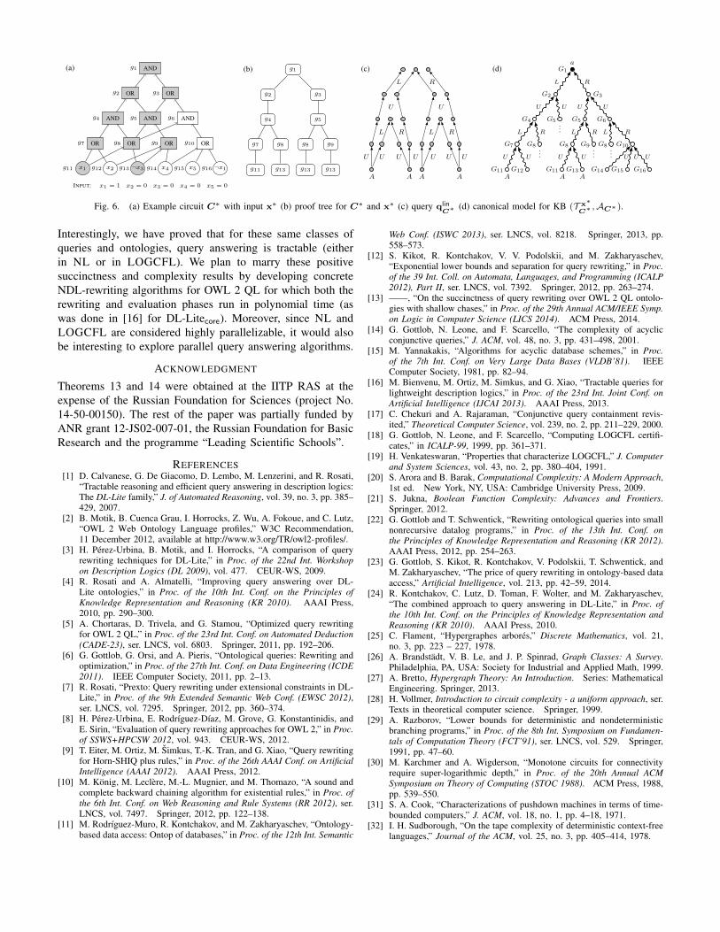
corresponding literal evaluates into 1 under x.For example, the circuit C∗ in Fig. 6(a) accepts input x∗ =(1, 0, 0, 0, 1), as witnessed by the proof tree in Fig. 6(b).

Importantly, while a circuit-input pair may admit multipleproof trees, they are all isomorphic modulo the labelling. Thus,with every circuit C, we can associate a skeleton proof treeTC such that C accepts input x iff some labelling of TC isa proof tree for C and x. The reduction in [14] encodes thecircuit C and input x in the database and uses a Booleantree-shaped query based upon the skeleton proof tree. Moreprecisely, the database Dx

C uses the gates of C as constantsand contains the following facts2:• U(gj , gi), for every OR gate gi with predecessor gate gj ;• L(gj , gi) (resp. R(gj , gi)), for every AND gate gi with

left (resp. right) predecessor gj ;• A(gi), for every input gate gi whose value is 1 under x.

The query qC uses the nodes of TC as variables, has an atomU(nj , ni) (resp. L(nj , ni), R(nj , ni)) for every node ni withunique (resp. left, right) child nj , and has an atom A(ni) forevery leaf node ni. It is proven in [14] that Dx

C |= qC ifand only if C accepts x. Moreover, both qC and Dx

C can beconstructed by means of logspace transducers.

To adapt the preceding reduction to our setting, we willreplace the tree-shaped query qC by a linear query qlin

C that

2For presentation purposes, we use a minor variant of the reduction in [14].

is obtained, intuitively, by performing an ordered depth-firsttraversal of qC . The new query qlin

C may give a differentanswer than qC when evaluated on Dx

C , but the two queriescoincide if evaluated on the unraveling of Dx

C into a tree.Thus, we will define a KB (T x

C ,AC) whose canonical modelinduces a tree that is isomorphic to the tree-unravelling of Dx

C .To formally define the query qlin

C , consider the sequence ofwords inductively defined as follows: w0 = ε and wj+1 =L− U− wj U LR− U− wj U R. Every word w = %1%2 . . . %knaturally gives rise to a linear query qw =

∧ki=1 %i(yi−1, yi).

We then take

qlinC = ∃y1 . . . ∃yk(qwd ∧

∧wn[i,i+1]=U− U

A(yi)).

where k = |wd| and d is such that C has 2d + 1 levels. Thequery qlin

C∗ for our example circuit C∗ is given in Fig. 6(c).We now proceed to the definition of the KB (T x

C ,AC).Suppose C has gates g1, g2, . . . , gm, with g1 the output gate. Inaddition to the predicates U,L,R,A from earlier, we introducea unary predicate Gi for each gate gi and a binary predicate Pijfor each gate gi with predecessor gj . We set AC = G1(a)and include in T x

C the following axioms:• Gi(x) → ∃yPij(y, x) and ∃yPij(x, y) → Gj(x) for

every gate gi with predecessor gj ;• Pij(x, y) → S(x, y) for every S ∈ U,L,R such thatS(gj , gi) ∈ Dx

C ;• Gi(x)→ A(x) whenever A(gi) ∈ Dx

C .In Fig. 6(d), we display (a portion of) the canonical model ofthe KB associated with circuit C∗ and input x∗. Observe that,when restricted to the predicates U,L,R,A, it is isomorphicto the unravelling of Dx

C into a tree starting from g1.In the appendix, we argue qlin

C and (T xC ,AC) can be con-

structed by logspace transducers, and we prove the followingproposition that establishes the correctness of the reduction.

Proposition 24. C accepts input x iff T xC ,AC |= qlin

C (a).

V. CONCLUSION

In this paper, we have clarified the impact of query topologyand ontology depth on the worst-case size of query rewritingsand the complexity of query answering in OWL 2 QL. Ourresults close an open question from [13] and yield a completepicture of the succinctness and complexity landscapes for theconsidered classes of queries and ontologies.

On the theoretical side, our results demonstrate the utilityof using non-uniform complexity as a tool for studying suc-cinctness. In future work, we plan to utilize the developedmachinery to investigate additional dimensions of the suc-cinctness landscape, with the hope of identifying other naturalrestrictions that guarantee small rewritings.

Our results also have practical implications for queryingOWL 2 QL KBs. Indeed, our succinctness analysis providesstrong evidence in favour of adopting NDL as the targetlanguage for rewritings, since we have identified a range ofquery-ontology pairs for which polysize NDL-rewritings areguaranteed, but PE-rewritings may be of superpolynomial size.

(a)

x1g11 x2g12 ¬x3g13 x4g14 x5g15 ¬x1g16

INPUT: x1 = 1 x2 = 0 x3 = 0 x4 = 0 x5 = 0

ORg7 ORg8 ORg9 ORg10

ANDg4 ANDg5 ANDg6

ORg2 ORg3

ANDg1 (b)

g11

g7

g13

g8

g4

g2

g1

g3

g5

g8 g9

g13 g13

(c)

A A A A

U

U U

L R

U U

L R

U

U

L R

U U

(d)

G11AG12 G11

AG13

AG14 G15 G16

G7 G8...

G8 G9...

G8...

G10

G4 G5...

G5 G6

G2 G3

G1

a

L R

U U U U

L R L R L R

U U U U U U U

Fig. 6. (a) Example circuit C∗ with input x∗ (b) proof tree for C∗ and x∗ (c) query qlinC∗ (d) canonical model for KB (T x∗

C∗ ,AC∗ ).

Interestingly, we have proved that for these same classes ofqueries and ontologies, query answering is tractable (eitherin NL or in LOGCFL). We plan to marry these positivesuccinctness and complexity results by developing concreteNDL-rewriting algorithms for OWL 2 QL for which both therewriting and evaluation phases run in polynomial time (aswas done in [16] for DL-Litecore). Moreover, since NL andLOGCFL are considered highly parallelizable, it would alsobe interesting to explore parallel query answering algorithms.

ACKNOWLEDGMENT

Theorems 13 and 14 were obtained at the IITP RAS at theexpense of the Russian Foundation for Sciences (project No.14-50-00150). The rest of the paper was partially funded byANR grant 12-JS02-007-01, the Russian Foundation for BasicResearch and the programme “Leading Scientific Schools”.

REFERENCES[1] D. Calvanese, G. De Giacomo, D. Lembo, M. Lenzerini, and R. Rosati,

“Tractable reasoning and efficient query answering in description logics:The DL-Lite family,” J. of Automated Reasoning, vol. 39, no. 3, pp. 385–429, 2007.

[2] B. Motik, B. Cuenca Grau, I. Horrocks, Z. Wu, A. Fokoue, and C. Lutz,“OWL 2 Web Ontology Language profiles,” W3C Recommendation,11 December 2012, available at http://www.w3.org/TR/owl2-profiles/.

[3] H. Perez-Urbina, B. Motik, and I. Horrocks, “A comparison of queryrewriting techniques for DL-Lite,” in Proc. of the 22nd Int. Workshopon Description Logics (DL 2009), vol. 477. CEUR-WS, 2009.

[4] R. Rosati and A. Almatelli, “Improving query answering over DL-Lite ontologies,” in Proc. of the 10th Int. Conf. on the Principles ofKnowledge Representation and Reasoning (KR 2010). AAAI Press,2010, pp. 290–300.

[5] A. Chortaras, D. Trivela, and G. Stamou, “Optimized query rewritingfor OWL 2 QL,” in Proc. of the 23rd Int. Conf. on Automated Deduction(CADE-23), ser. LNCS, vol. 6803. Springer, 2011, pp. 192–206.

[6] G. Gottlob, G. Orsi, and A. Pieris, “Ontological queries: Rewriting andoptimization,” in Proc. of the 27th Int. Conf. on Data Engineering (ICDE2011). IEEE Computer Society, 2011, pp. 2–13.

[7] R. Rosati, “Prexto: Query rewriting under extensional constraints in DL-Lite,” in Proc. of the 9th Extended Semantic Web Conf. (EWSC 2012),ser. LNCS, vol. 7295. Springer, 2012, pp. 360–374.

[8] H. Perez-Urbina, E. Rodrıguez-Dıaz, M. Grove, G. Konstantinidis, andE. Sirin, “Evaluation of query rewriting approaches for OWL 2,” in Proc.of SSWS+HPCSW 2012, vol. 943. CEUR-WS, 2012.

[9] T. Eiter, M. Ortiz, M. Simkus, T.-K. Tran, and G. Xiao, “Query rewritingfor Horn-SHIQ plus rules,” in Proc. of the 26th AAAI Conf. on ArtificialIntelligence (AAAI 2012). AAAI Press, 2012.

[10] M. Konig, M. Leclere, M.-L. Mugnier, and M. Thomazo, “A sound andcomplete backward chaining algorithm for existential rules,” in Proc. ofthe 6th Int. Conf. on Web Reasoning and Rule Systems (RR 2012), ser.LNCS, vol. 7497. Springer, 2012, pp. 122–138.

[11] M. Rodrıguez-Muro, R. Kontchakov, and M. Zakharyaschev, “Ontology-based data access: Ontop of databases,” in Proc. of the 12th Int. Semantic

Web Conf. (ISWC 2013), ser. LNCS, vol. 8218. Springer, 2013, pp.558–573.

[12] S. Kikot, R. Kontchakov, V. V. Podolskii, and M. Zakharyaschev,“Exponential lower bounds and separation for query rewriting,” in Proc.of the 39 Int. Coll. on Automata, Languages, and Programming (ICALP2012), Part II, ser. LNCS, vol. 7392. Springer, 2012, pp. 263–274.

[13] ——, “On the succinctness of query rewriting over OWL 2 QL ontolo-gies with shallow chases,” in Proc. of the 29th Annual ACM/IEEE Symp.on Logic in Computer Science (LICS 2014). ACM Press, 2014.

[14] G. Gottlob, N. Leone, and F. Scarcello, “The complexity of acyclicconjunctive queries,” J. ACM, vol. 48, no. 3, pp. 431–498, 2001.

[15] M. Yannakakis, “Algorithms for acyclic database schemes,” in Proc.of the 7th Int. Conf. on Very Large Data Bases (VLDB’81). IEEEComputer Society, 1981, pp. 82–94.

[16] M. Bienvenu, M. Ortiz, M. Simkus, and G. Xiao, “Tractable queries forlightweight description logics,” in Proc. of the 23rd Int. Joint Conf. onArtificial Intelligence (IJCAI 2013). AAAI Press, 2013.

[17] C. Chekuri and A. Rajaraman, “Conjunctive query containment revis-ited,” Theoretical Computer Science, vol. 239, no. 2, pp. 211–229, 2000.

[18] G. Gottlob, N. Leone, and F. Scarcello, “Computing LOGCFL certifi-cates,” in ICALP-99, 1999, pp. 361–371.

[19] H. Venkateswaran, “Properties that characterize LOGCFL,” J. Computerand System Sciences, vol. 43, no. 2, pp. 380–404, 1991.

[20] S. Arora and B. Barak, Computational Complexity: A Modern Approach,1st ed. New York, NY, USA: Cambridge University Press, 2009.

[21] S. Jukna, Boolean Function Complexity: Advances and Frontiers.Springer, 2012.

[22] G. Gottlob and T. Schwentick, “Rewriting ontological queries into smallnonrecursive datalog programs,” in Proc. of the 13th Int. Conf. onthe Principles of Knowledge Representation and Reasoning (KR 2012).AAAI Press, 2012, pp. 254–263.

[23] G. Gottlob, S. Kikot, R. Kontchakov, V. Podolskii, T. Schwentick, andM. Zakharyaschev, “The price of query rewriting in ontology-based dataaccess,” Artificial Intelligence, vol. 213, pp. 42–59, 2014.

[24] R. Kontchakov, C. Lutz, D. Toman, F. Wolter, and M. Zakharyaschev,“The combined approach to query answering in DL-Lite,” in Proc. ofthe 10th Int. Conf. on the Principles of Knowledge Representation andReasoning (KR 2010). AAAI Press, 2010.

[25] C. Flament, “Hypergraphes arbores,” Discrete Mathematics, vol. 21,no. 3, pp. 223 – 227, 1978.

[26] A. Brandstadt, V. B. Le, and J. P. Spinrad, Graph Classes: A Survey.Philadelphia, PA, USA: Society for Industrial and Applied Math, 1999.

[27] A. Bretto, Hypergraph Theory: An Introduction. Series: MathematicalEngineering. Springer, 2013.

[28] H. Vollmer, Introduction to circuit complexity - a uniform approach, ser.Texts in theoretical computer science. Springer, 1999.

[29] A. Razborov, “Lower bounds for deterministic and nondeterministicbranching programs,” in Proc. of the 8th Int. Symposium on Fundamen-tals of Computation Theory (FCT’91), ser. LNCS, vol. 529. Springer,1991, pp. 47–60.

[30] M. Karchmer and A. Wigderson, “Monotone circuits for connectivityrequire super-logarithmic depth,” in Proc. of the 20th Annual ACMSymposium on Theory of Computing (STOC 1988). ACM Press, 1988,pp. 539–550.

[31] S. A. Cook, “Characterizations of pushdown machines in terms of time-bounded computers,” J. ACM, vol. 18, no. 1, pp. 4–18, 1971.

[32] I. H. Sudborough, “On the tape complexity of deterministic context-freelanguages,” Journal of the ACM, vol. 25, no. 3, pp. 405–414, 1978.

PROOFS FOR SECTION II

Theorem 5. Thm. 4 remains true if f twq,T is replaced by f tw′

q,T :

f tw′

q,T =∨

Θ⊆ΘqT

independent

( ∧η∈q\qΘ

pη ∧∧t∈Θ

( ∧z,z′∈t

pz=z′ ∧∨

%∈N±2 ,t∈ΘqT [%]

∧z∈t

p%z))

Remark. In fact, Theorem 4 was proved in [13] only for consistent KBs. However, it is known that it is possible to definea short PE-query q⊥T that when evaluated on IA returns all k-tuples of individual constants on IA if the KB (T ,A) isinconsistent, and returns no answers otherwise, cf. [33]. It follows that if q′ is a rewriting for q and T for all data instancesA that are consistent with T , then we can obtain a rewriting for q and T (that works for all data instances) by taking thedisjunction of q′ and q⊥T . Therefore, to prove Theorem 5, it sufficient to show how to construct such “consistent rewritings”.

Proof. Let T be an OWL 2 QL ontology and q = ∃yϕ(x,y) be a CQ with answer variables x and existential variables y.(we will use z and z′ when referring to variables of either type). We begin by recalling that every atom η(u) has the followingsimple PE-rewriting:

ρη =∨

T |=ξ(u)→η(u)

ξ(u)

where ξ(u) ranges over %(u) (% ∈ N±2 ) when |u| = 2 and over

τ(u) ::= A(u) (A ∈ N1) | ∃v %(u, v) (% ∈ N±2 )

when u consists of the single variable u.

To show the first statement, consider a Boolean formula χ that computes f tw′

q,T , and let q′ be the FO-formula obtained fromχ as follows:• replace pz=z′ by the equality z = z′;• replace pη by its PE-rewriting ρη;• replace p%z by the PE-rewriting ρ%(z) of ∃y%(z, y);• existentially quantify the variables y.

Note that q′ has the same answer variables as q, and if χ is a monotone formula, then q′ is a PE-formula.We wish to show that q′ is a consistent rewriting of q and T (cf. preceding remark). To do so, we let q′′ be the PE-formula

obtained by applying the above transformation to the original monotone Boolean formula f tw′

q,T :

q′′ = ∃y∨

Θ⊆ΘqT

independent

( ∧η∈q\qΘ

ρη ∧∧t∈Θ

(∧

z,z′∈tz = z′ ∧

∨%∈N±2 ,t∈ΘqT [%]

∧z∈t

ρ%(z))

).

We know that χ and f tw′

q,T compute the same Boolean function. It follows that q′ and q′′ are equivalent FO-formulas. It thussuffices to show that q′′ is a consistent rewriting of q and T . This is easily seen by comparing q′′ to the following query

q′′′ = ∃y′∨

Θ⊆ΘqT

independent

( ∧η∈q\qΘ

ρη ∧∧t∈Θ

(∨

%∈N±2 ,t∈ΘqT [%]

∃z ( ρ%(z) ∧∧z′∈tr

z′ = z))

)

which was proven in [13] to be a consistent FO-rewriting of q and T (here y′ is the restriction of y to the variables in q′′′).

The proof of the second statement concerning NDL-rewritings closely follows the proof of Theorem 4 from [], but weinclude it for the sake of completeness. First, we define a unary predicate D0 that contains all individual constants of the givendata instance. This is done by taking the rules

%(u)→ D0(u), (2)

where %(u) is of the form S(u), S(u, v) and S(v, u), for some predicate S ∈ sig(T ) ∪ sig(q). Next, we let z = x ∪ y anddefine a |z|-ary predicate D using the following rule:∧

z∈zD0(z)→ D(z). (3)

We need the predicate D to ensure that all the rules in our NDL program are safe, i.e. every variable that appears in the headof a rule also occurs in the body.

Now let C be a monotone circuit for f twq,T whose gates are g1, . . . , gn, with gn the output gate. For input gates gi whosevariable is pz=z′ , we take the rule3

z = z′ ∧D(z)→ Gi(z). (4)

For every input gate gi whose variable is pη , we include the rule

ξ ∧D(z)→ Gi(z), (5)

for every disjunct ξ of the rewriting ρη(z) of η and T (here we assume w.lo.g. that any variable in ξ that does not appear inν does not belong to z). If instead gi is associated with variable p%z , then we use the rules

ξ ∧D(z)→ Gi(z), (6)

where ξ is a disjunct of the rewriting ρ% of %(z) and T (here again we assume that every variable that appears both in ξ andz also appears in the atom %). The remaining (AND and OR) gates are encoded using the following rules:

Gj1(z) ∧Gj2(z) ∧D(z)→ Gi(z) if gi = gj1 ∧ gj2 ; (7)

Gj1(z) ∧D(z)→ Gi(z)

Gj2(z) ∧D(z)→ Gi(z)

if gi = gj1 ∨ gj2 . (8)

Denote the resulting set of rules (2)–(8) by Π. We note that Π is of size O(|C| · |T |) and further claim that (Π, Gn) isan NDL-rewriting of q and T . To see why, observe that by “unfolding” these rules in the standard way, we can transform(Π, Gn) into an equivalent PE-formula of the form

∃y[ψ(x,y) ∧

∧z∈Z

( ∨%(u)→D0(u)∈Π

%(z))],

where Z ⊆ x∪y and ∃yψ(x,y) can be constructed by taking the Boolean formula representing C and replacing pη with ρη ,pz=z′ with z = z′ and p%z with ρ%. We have already shown that ∃yψ(x,y) is a rewriting of q and T in the first half of theproof, and the additional conjuncts asserting that the variables in z appear in some predicate are trivially satisfied.

Theorem 6 If q′ is a (PE-) FO-rewriting of q and T , then there is a (monotone) Boolean formula χ of size O(|q′|) whichcomputes fprimq,T . If (Π, G) is an NDL-rewriting of q and T , then fprimq,T is computed by a monotone Boolean circuit C of sizeO(|Π|).

Proof (implicit in [13]). Given a PE-, FO- or NDL-rewriting q′ of q and T , we show how to construct, respectively, a monotoneBoolean formula, a Boolean formula or a monotone Boolean circuit for the function fprimq,T of size |q′|.

Suppose q′ is a PE-rewriting of q and T . We eliminate the quantifiers in q′ by first replacing every subformula of the form∃xψ(x) in q′ with ψ(a), and then replacing each atom of the form A(a) and P (a, a) with the corresponding propositionalvariable. One can verify that the resulting propositional monotone Boolean formula computes fprimq,T . If q′ is an FO-rewriting ofq, then we eliminate the quantifiers by replacing ∃xψ(x) and ∀xψ(x) in q′ with ψ(a). We then proceed as before, replacingatoms A(a) and P (a, a) by the corresponding propositional variables, to obtain a Boolean formula computing fprimq,T .

If (Π, G) is an NDL-rewriting of q, then we replace all the variables in Π with a and then perform the replacement describedabove. Denote the resulting propositional NDL-program by Π′. The program Π′ can now be transformed into a monotoneBoolean circuit computing fprimq,T . For every (propositional) variable p occurring in the head of a rule in Π′, we introduce anOR-gate whose output is p and inputs are the bodies of the rules with head p; for each such body, we introduce an AND-gatewhose inputs are the propositional variables in the body.

PROOFS FOR SECTION III

Theorem 8. Let P = (HP , lP ) be a THGP. For every input α for P , fP (α) = 1 iff fprimqP ,TP (γ) = 1, where γ is defined asfollows: γ(Be) = 1, γ(Re) = γ(R′e) = 0, and γ(Sij) = γ(S′ij) = α(lP (vi, vj)).

Proof. Consider a THGP P = (HP , lP ) whose underlying tree T has vertices v1, . . . , vn, and let T ↓ be the directed treeobtained from T by fixing one of its leaves v1 as the root and orienting edges away from v1. In what follows, we will saythat a vertex v ∈ VT is an internal vertex in e ∈ EP (w.r.t. T ) if it appears in e and is neither a leaf nor a boundary vertexof e w.r.t. T . Note that because we chose a leaf as root of T ↓, we know that for every hyperedge e, the highest vertex in e(according to T ↓) must be either a leaf or a boundary vertex of e.

3For ease of notation, we use equality atoms in rule bodies, but these can be removed using standard (equality-preserving) transformations.

Take some α : LP → 0, 1 and let γ be as defined in the theorem statement. Define the corresponding data instance:

Aγ = Be(a) | e ∈ EP ∪ Sij(a, a), S′ij(a, a) | γ(Sij) = γ(S′ij) = α(lP (vi, vj)) = 1.

For the first direction, suppose that fP (α) = 1. Then we know that there exists E′ ⊆ EP that is independent and covers allzeros of α. To show fprimqP ,TP (γ) = 1, we must show that TP ,Aγ |= qP . Define a mapping h as follows:• h(yi) = aReR

′e if vi is an internal vertex of e ∈ E′. Otherwise, h(yi) = a.

• h(yij) = aRe if vi, vj ∈ e and e ∈ E′. Otherwise, h(yij) = a.Note that h is well-defined: since E′ is independent, different hyperedges in E′ cannot share internal vertices, and there canbe at most one hyperedge e ∈ E′ that contains a given edge vi, vj.

It remains to show that h is a homomorphism from qP to CTP ,Aγ . Consider a pair of atoms Sij(yi, yij), S′ij(yij , yj) in qP .Then (vi, vj) ∈ T ↓, so either α(vi, vj) = 1 or there is some e ∈ E′ such that vi, vj ∈ e.

In the former case, we have γ(Sij) = γ(S′ij) = 1, so Aγ contains Sij(a, a) and S′ij(a, a). If there is no e ∈ E′ such thatvi, vj ∈ e, then h(yi) = h(yij) = h(yj) = a, so the atoms Sij(yi, yij), S′ij(yij , yj) are satisfied by h.

Now consider the alternative in which e = 〈vk1 , . . . , vkm〉 ∈ E′ is such that vi, vj ∈ e and e ∈ E′. Note that becauseboundary vertices must have degree 2 (recall that this condition is part of the definition of THGPs), we know that all boundaryand leaf vertices of e must be among vk1 , . . . , vkm . Moreover, we may assume without loss of generality that vk1 , . . . , vkmare all either boundary vertices or leaves of T (since any internal vertex vk` can be dropped without changing the meaning ofe). Note that this ensures that for all vi ∈ e, h(yi) = a iff vi ∈ vk1 , . . . , vkm. There are four possibilities to consider:• Case 1: vi, vj ⊆ vk1 , . . . , vkm (i.e. neither of vi and vj is internal). We know that the boundary vertices of e have

degree 2, so the only possibility is that e = vi, vj. We therefore have h(vi) = h(vj) = a and h(vij) = aRe, and theontology TP contains Re(x, y)→ Sij(x, y) and Re(y, x)→ S′ij(x, y).

• Case 2: vi ∈ vk1 , . . . , vkm but vj 6∈ vk1 , . . . , vkm. (i.e. vi is a boundary vertex or leaf and vj is internal)

We have h(vi) = a, h(vij) = aRe, and h(vj) = aReR′e, and the ontology contains Re(x, y)→ Sij(x, y) and R′e(x, y)→

S′ij(x, y).

• Case 3: vj ∈ vk1 , . . . , vkm but vi 6∈ vk1 , . . . , vkm (i.e. vj is a boundary vertex or leaf and vi is internal)

Then we have h(vj) = a, h(vij) = aRe, and h(vi) = aReR′e, and the ontology contains Re(y, x) → S′ij(x, y) and

R′e(y, x)→ Sij(x, y).

• Case 4: vi, vj ∩ vk1 , . . . , vkm = ∅ (i.e. both are internal vertices). Then we have h(vi) = h(vj) = aReR′e and

h(vij) = aRe, and the ontology contains Re(y, x)→ Sij(x, y) and R′e(x, y)→ S′ij(x, y).In all cases, we find that h satisfies the atoms Sij(yi, yij), S′ij(yij , yj). We can thus conclude that h is indeed a homomorphism.

For the other direction, suppose that fprimqP ,TP (α) = 1. Then we have TP ,Aγ |= qP , so there is a homomorphism h : qP →CTP ,Aγ . We wish to show that there exists a subset of EP that is independent and covers all zeros of α. Let us define E′ asthe set of all e ∈ E such that h−1(aRe) 6= ∅ (that is, aRe is in the image of h).

To show that E′ is independent, we start by establishing the following claim:

Claim. If h−1(aRe) 6= ∅, yij ∈ vars(qH), and vi, vj ∈ e, then h(yij) = aRe.

Proof of claim. Suppose that h−1(aRe) 6= ∅, where e = 〈vk1 , . . . , vkm〉 ∈ E′. We may assume w.l.o.g. that vk1 is the highestvertex in e according to T ′, and that none of vk1 , . . . , vkm is an internal vertex. Now pick some variable z ∈ h−1(aRe) suchthat there is no z′ ∈ h−1(aRe) that is higher than z in qP (here we use the ordering of variables induced by the tree T ↓). Wefirst note that z cannot be of the form yj , since then there is an atom in qP of the form Sj`(yj , yj`) or S′`j(y`j , yj), and aRedoes not have any outgoing Sj` or S′−`j arcs in CTP ,Aγ . It follows that z = yj`. By again considering the available arcs leavingaRe, we can further see that vj , v` ∈ e. We next wish to show that j = k1. Suppose that this is not the case. Then, we knowthat there must exist some edge vp, vj ∈ e such that (vp, vj) ∈ T ↓. A simple examination of the axioms in TP shows thatthe only way for h to satisfy the atom Sj`(yj , yj`) is to map yj to aReR

′e. It follows that to satisfy that atom S′pj(ypj , yj),

we must have h(ypj) = aRe. This contradicts our earlier assumption that z = yj` was a highest vertex in h−1(aRe). We thushave j = k1. Now using a simple inductive argument on the distance from yk1 , and considering the possible ways of mappingthe atoms of qH , we can show that h(yij) = aRe for every vi, vj ∈ e. (end proof of claim)

Suppose that there are two distinct hyperedges e, e′ ∈ E′ that have a non-empty intersection: vi, vj ∈ e ∩ e′. We knowthat either yij or yji belongs to vars(qP ), and we can suppose w.l.o.g. that it is the former. We can thus apply the precedingclaim to obtain h(yij) = aRe = aRe′ , a contradiction. We have thus shown that E′ is independent, and so it only remains toshow it covers all zeros. To this end, let vi, vj be such that α(vi, vj) = 0 and again suppose w.l.o.g. that yij ∈ vars(qP ).Then Aγ does not contain Sij(a, a), so the only way h can satisfy the query atom Sij(yi, yij) is by mapping yij to some

element aRe such that vi, vj ∈ e. It follows that there is some e ∈ E′ such that vi, vj ∈ e, so all zeros of α are coveredby E′. We have thus shown that E′ is an independent subset of EP that covers all zeros of α, and hence we conclude thatfP (α) = 1.

Theorem 9. Fix t ≥ 1 and d ≥ 0. For every ontology T of depth ≤ d and CQ q of treewidth ≤ t, there is a monotone THGPthat computes f tw

′

q,T of size polynomial in |T |+ |q|.

More specifically, we show the following:

Proposition. For every ontology T and CQ q, the THGP (Hq,T , lq,T ) defined in Section III.C computes f tw′

q,T . If T has depthd and q has treewidth t, then Hq,T• contains at most (2M + 1)L vertices;• contains at most L(M +M2) hyperedges;• has labels with at most (2|T |+ |q|+ 1)|q| conjuncts.

where L = (2|q| − 1)2 and M = |W td| ≤ (2|T |)d.

Proof. Let (T, λ) be the tree decomposition of Gq of width t that was used to construct the THGP (Hq,T , lq,T ). We mayassume w.l.o.g. that T contains at most (2|q| − 1)2 nodes, cf. [34]. Recall that to more easily refer to the variables in λ(N),we make use of functions λ1, . . . , λt such that λi(N) ∈ λ(N) and λ(N) = ∪iλi(N). Further recall that the formula f tw

′

q,T isdefined as follows:

f tw′

q,T =∨

Θ⊆ΘqT

independent

( ∧η∈q\qΘ

pη ∧∧t∈Θ

( ∧z,z′∈t

pz=z′ ∧∨

%∈N±2 ,t∈ΘqT [%]

∧z∈t

p%z))

where qΘ =⋃

t qt. Throughout the proof, we use fP to denote the function computed by the THGP (Hq,T , lq,T ). Note thatby definition fP uses exactly the same set of propositional variables as f tw

′

q,T .

To show the first direction of the first statement, let v be a valuation of the variables in f tw′

q,T such that f tw′

q,T (v) = 1. Thenwe can find an independent subset Θ ⊆ Θq

T such that v satisfies the corresponding disjunct of f tw′

q,T :∧η∈q\qΘ

pη ∧∧t∈Θ

( ∧z,z′∈t

pz=z′ ∧∨

%∈N±2 ,t∈ΘqT [%]

∧z∈t

p%z)

(9)

For every t ∈ Θ, we let %t be a role that makes the final disjunction hold. Furthermore, we choose some homomorphismht : qt → CT%t ,A%t , where T%t = T ∪ A%t(x)→ ∃y%t(x, y) and A%t = A%t(a). Such homomorphisms are guaranteed toexist by the definition of tree witnesses.

Now for each node N in the tree decomposition T , we define wN by setting:• wN [j] = ε if λj(N) = z and either z appears in an atom η such that v(pη) = 1 or there is some t ∈ Θ such that z ∈ tr.• wN [j] = w if λj(N) = z and there is some t ∈ Θ such that z ∈ ti and ht(z) = aw.

First note that wN is well-defined since the independence of Θ guarantees that every variable in q can appear in ti for at mostone tree witness t ∈ Θ. Moreover, every variable in q must either belong to an atom η such that v(pη) = 1 or to an atom thatis contained in qt for some t ∈ Θ.

Next we show that wN is consistent with the node N . To show that the first condition holds, consider some atom A(λi(N)) ∈q such that wN [i] 6= ε. Then there must be a tree witness t ∈ Θ such that λi(N) ∈ ti, in which case we have thatht(λi(N)) = awN [i]. Let ς ∈ N±2 be the final symbol in wN [i]. Then since ht is a homomorphism from qt into CT%t ,A%t , itmust be the case that T |= ∃y ς(y, x)→ A(x).

To show the second condition holds, consider some atom R(λi(N), λj(N)) ∈ q such that either wN [i] 6= ε or wN [j] 6= ε.We suppose w.l.o.g. that wN [i] 6= ε (the other case is handled analogously). It follows from the definition of wN that theremust exist a tree witness t ∈ Θ such that λi(N) ∈ ti and ht(λi(N)) = awN [i]. Since λi(N) ∈ ti and R(λi(N), λj(N)) ∈ q,the definition of tree witnesses ensures that λj(N) ∈ t. Because ht is a homomorphism from qt into CT%t ,A%t , we know thatone of the following must hold:• λj(N) ∈ tr, wN [j] = ε, and wN [i] = ς for some ς ∈ N±2 such that T |= ς(y, x)→ R(x, y)• λj(N) ∈ ti and wN [i] = wN [j] · ς for some ς ∈ N±2 such that T |= ς(y, x)→ R(x, y)• λj(N) ∈ ti and wN [j] = wN [i] · ς for some ς ∈ N±2 such that T |= ς(x, y)→ R(x, y)

This establishes the second consistency condition.

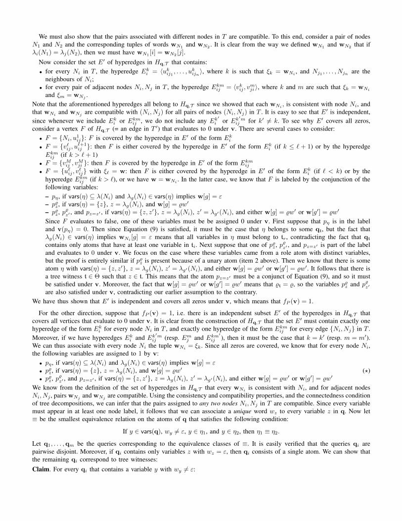
We must also show that the pairs associated with different nodes in T are compatible. To this end, consider a pair of nodesN1 and N2 and the corresponding tuples of words wN1 and wN2 . It is clear from the way we defined wN1 and wN2 that ifλi(N1) = λj(N2), then we must have wN1 [i] = wN2 [j].

Now consider the set E′ of hyperedges in Hq,T that contains:• for every Ni in T , the hyperedge Eki = 〈ukij1 , . . . , u

kijn〉, where k is such that ξk = wNi , and Nj1 , . . . , Njn are the

neighbours of Ni;• for every pair of adjacent nodes Ni, Nj in T , the hyperedge Ekmij = 〈vkij , vmji 〉, where k and m are such that ξk = wNi

and ξm = wNj .Note that the aforementioned hyperedges all belong to Hq,T since we showed that each wNi , is consistent with node Ni, andthat wNi and wNj are compatible with (Ni, Nj) for all pairs of nodes (Ni, Nj) in T . It is easy to see that E′ is independent,since whenever we include Eki or Ekmij , we do not include any Ek

′i or Ek

′mij for k′ 6= k. To see why E′ covers all zeros,

consider a vertex F of Hq,T (= an edge in T ′) that evaluates to 0 under v. There are several cases to consider:• F = Ni, u1

ij: F is covered by the hyperedge in E′ of the form Eki• F = v`ij , u

`+1ij : then F is either covered by the hyperedge in E′ of the form Eki (if k ≤ ` + 1) or by the hyperedge

Ekmij (if k > `+ 1)• F = vMij , vMji : then F is covered by the hyperedge in E′ of the form Ekmij• F = u`ij , v`ij with ξ` = w: then F is either covered by the hyperedge in E′ of the form Eki (if ` < k) or by the

hyperedge Ekmij (if k > `), or we have w = wNi . In the latter case, we know that F is labeled by the conjunction of thefollowing variables:– pη , if vars(η) ⊆ λ(Ni) and λg(Ni) ∈ vars(η) implies w[g] = ε– p%z , if vars(η) = z, z = λg(Ni), and w[g] = %w′

– p%z , p%z′ , and pz=z′ , if vars(η) = z, z′, z = λg(Ni), z′ = λg′(Ni), and either w[g] = %w′ or w[g′] = %w′

Since F evaluates to false, one of these variables must be be assigned 0 under v. First suppose that pη is in the labeland v(pη) = 0. Then since Equation (9) is satisfied, it must be the case that η belongs to some qt, but the fact thatλg(Ni) ∈ vars(η) implies wNi [g] = ε means that all variables in η must belong to tr, contradicting the fact that qt

contains only atoms that have at least one variable in ti. Next suppose that one of p%z , p%z′ , and pz=z′ is part of the labeland evaluates to 0 under v. We focus on the case where these variables came from a role atom with distinct variables,but the proof is entirely similar if p%z is present because of a unary atom (item 2 above). Then we know that there is someatom η with vars(η) = z, z′, z = λg(Ni), z′ = λg′(Ni), and either w[g] = %w′ or w[g′] = %w′. It follows that there isa tree witness t ∈ Θ such that z ∈ t. This means that the atom pz=z′ must be a conjunct of Equation (9), and so it mustbe satisfied under v. Moreover, the fact that w[g] = %w′ or w[g′] = %w′ means that %t = %, so the variables p%z and p%z′are also satisfied under v, contradicting our earlier assumption to the contrary.

We have thus shown that E′ is independent and covers all zeros under v, which means that fP (v) = 1.

For the other direction, suppose that fP (v) = 1, i.e. there is an independent subset E′ of the hyperedges in Hq,T thatcovers all vertices that evaluate to 0 under v. It is clear from the construction of Hq,T that the set E′ must contain exactly onehyperedge of the form Eki for every node Ni in T , and exactly one hyperedge of the form Ekmij for every edge Ni, Nj in T .Moreover, if we have hyperedges Eki and Ek

′mij (resp. Emj and Ekm

′ij ), then it must be the case that k = k′ (resp. m = m′).

We can thus associate with every node Ni the tuple wNi = ξk. Since all zeros are covered, we know that for every node Ni,the following variables are assigned to 1 by v:• pη , if vars(η) ⊆ λ(Ni) and λg(Ni) ∈ vars(η) implies w[g] = ε• p%z , if vars(η) = z, z = λg(Ni), and w[g] = %w′ (?)• p%z , p%z′ , and pz=z′ , if vars(η) = z, z′, z = λg(Ni), z′ = λg′(Ni), and either w[g] = %w′ or w[g′] = %w′

We know from the definition of the set of hyperedges in Hq,T that every wNi is consistent with Ni, and for adjacent nodesNi, Nj , pairs wNj and wNj are compatible. Using the consistency and compatibility properties, and the connectedness conditionof tree decompositions, we can infer that the pairs assigned to any two nodes Ni, Nj in T are compatible. Since every variablemust appear in at least one node label, it follows that we can associate a unique word wz to every variable z in q. Now let≡ be the smallest equivalence relation on the atoms of q that satisfies the following condition:

If y ∈ vars(q), wy 6= ε, y ∈ η1, and y ∈ η2, then η1 ≡ η2.

Let q1, . . . ,qm be the queries corresponding to the equivalence classes of ≡. It is easily verified that the queries qi arepairwise disjoint. Moreover, if qi contains only variables z with wz = ε, then qi consists of a single atom. We can show thatthe remaining qi correspond to tree witnesses:Claim. For every qi that contains a variable y with wy 6= ε:

1) there is a role %i such that every wy 6= ε begins by %i2) there is a homomorphism hi from qi into CTi,Ai where Ti = T ∪A%i(x)→ ∃y%i(x, y) and Ai = A%i(a) (with A%i

fresh)3) there is a tree witness ti for q and T generated by %i such that qi = qti

Proof of claim. From the way we defined qi, we know that there exists a sequence Q0, . . . , Qm of subsets of q such thatQ0 = η0 ⊆ qi contains a variable y0 with wy0 6= ε, Qm = qi, and for every 1 ≤ ` ≤ m, Q`+1 is obtained from Q` byadding an atom η ∈ q \Q` that contains a variable y that appears in Q` and is such that wy 6= ε. By construction, every atomin qi contains a variable y with wy 6= ε. Let %i be the first letter of the word wy0 , and for every 0 ≤ ` ≤ m, let h` be thefunction mapping every variable z in Q` to awz .

Statements 1 and 2 can be shown by induction. The base case is trivial. For the induction step, suppose that at stage `,we know that every variable y in Q` with wy 6= ε begins by %i, and that h` is a homomorphism of Q` into the canonicalmodel CTi,Ai . We let η be the unique atom in Q`+1 \ Q`. Then we know that η contains a variable y that appears in Q`and is such that wy 6= ε. If η = B(y), then Statement 1 is immediate. For Statement 2, we let N be a node in T such thatvars(η) ⊆ λ(N) (such a node must exist by the definition of tree decompositions), and let j be such that λj(N) = y. We knowthat wN is consistent with N , so wy = wN [j] must end by a role ς with T |= ∃yς(y, x)→ B(x), which proves Statement 2.Next consider the other case in which η contains a variable other than y. Then η must be a role atom of the form η = R(y, z)or η = R(z, y). We give the argument for the case where η = R(y, z) (the argument for η = R(z, y) is entirely similar). LetN be a node in T such that vars(η) ⊆ λ(N), and let j, k be such that λj(N) = y and λk(N) = z. We know that wN isconsistent with N , so one of the following must hold:• wN [k] = wN [j] · ς with T |= ς(x, y)→ R(x, y)• wN [j] = wN [k] · ς with T |= ς(x, y)→ R(y, x)

By definition, we have wy = wN [j] and wz = wN [k]. Since wy begins with %i, it follows that the same holds for wz unlesswz = ε, which shows Statement 1. Moreover, we either have (i) wz = wyς and T |= ς(x, y) → R(x, y), or (ii) wy = wzςand T |= ς(x, y)→ R(y, x). In both cases, it is clear from the way we defined h`+1 that it is homomorphism from Q`+1 toCTi,Ai , so Statement 2 holds.

Statement 3 now follows from Statements 1 and 2, the definition of qi, and the definition of tree witnesses. (end proof ofclaim)

Let Θ consist of all the tree witnesses ti obtained from the preceding claim. As the qi are known to be disjoint, we havethat the set qti | ti ∈ Θ is independent. We aim to show that v satisfies the disjunct of f tw

′

q,T that corresponds to Θ (cf.Equation (9)). First consider some η ∈ q \ qΘ. Then we know that for every variable z in η, we have wz = ε. Let N be anode such that vars(η) ⊆ λ(N). Then we know that λg(N) ∈ vars(η) implies wN [g] = ε. It follows from (?) that v(pη) = 1.Next consider a variable pz=z′ such that there is an atom η ∈ ti with vars(η) = z, z′ such that z 6= z′. Then since η ∈ qi,we know that either wz 6= ε or wz′ 6= ε. It follows from (?) that v(pz=z′) = 1. Finally, consider some p%iz such that z ∈ ti.First suppose that there is a unary atom B(z) ∈ qti . Then we know that wz 6= ε, and so by the above claim, we must havewz = %iw

′. It follows that there is a node N in T such that z = λg(N) and wN [g] = %iw′. From (?), we can infer that p%iz

evaluates to 1 under v. The other possibility is that there exists a binary atom η ∈ qti such that vars(η) = z, z′. Let N bea node in T such that z = λg(N) and z′ = λg′(N). Since qti = qi, we know that either wz 6= ε or wz′ 6= ε. From the aboveclaim, this yields wN [g] = %iw

′ or wN [g′] = %iw′. We can thus apply (?) to obtain v(p%iz ) = 1. To conclude, we have shown

that v satisfies one of the disjuncts of f tw′

q,T , so f tw′

q,T (v) = 1.

For the second statement of the theorem, we recall that the tree T in the tree decomposition of q has at most (2|q| − 1)2

nodes and that the set W td consists of all tuples of words (w1, . . . , wt) | wi ∈ (N±2 ∩ sig(T ))∗, |wi| ≤ d. To simplify the

counting, we let L = (2|q| − 1)2 and M = |W td| ≤ (2|T |)d. The vertices of the hypergraph Hq,T correspond to the edges

of T ′, and there can be at most L · (2M + 1) of them, since there can be no more than L edges in T , and each is replacedby 2M + 1 new edges. The hyperedges of Hq,T are of two types: Eki (where 1 ≤ i ≤ L and 1 ≤ k ≤ M ) and Ekmij (where1 ≤ i ≤ L and 1 ≤ k ≤ M ). It follows that the total number of hyperedges cannot exceed L(M + M2). Finally, a simpleexamination of the labelling function shows that there can be at most (2|T |+ |q|+ 1)|q| conjuncts in each label.

Theorem 10. There exist polynomials p, p′ such that:• Every function computed by a semi-unbounded fan-in circuit of size at most σ and depth at most log σ is computable by

a THGP of size p(σ).• Every function computed by a THGP of size σ is computable by a semi-unbounded fan-in circuit of size at most p′(σ)

and depth at most log p′(σ).Both reductions preserve monotonicity.

(a) (b)

x1g1 x2g2

x3g3 x4g5ORg4

ANDg6 ANDg7

ORg8

v8 u8 w7 v7 u7 w6 v6 u6

w4 v4 u4 w2 v2 u2 w1 v1 u1

w5 v5 u5 w3 v3 u3

0 1 0 0 1 0 01

0 0 1 0 x1 1 0 x2

10 x4 1 0 x3

g7 = g4 ∧ g5

g4 = g1 ∨ g2

Fig. 7. (a) Example circuit, with nodes from S1 in white, nodes from S2 in grey (b) the tree underlying the corresponding THGP, together with labels andsome hyperedges

Proof of the First Statement of Theorem 10: THGPs can simulate SAC1 circuits

Consider a semi-unbounded fan-in circuit C of size at most σ and depth at most log σ. Denote its gates by g1, . . . , gσ ,where gσ is the output gate. We define the AND-depth of gates of C inductively. For the AND gate gi, its AND-depth, d(gi),equals 1 if on each path from gi to the input there are no AND gates. If there are AND gates on the paths from gi to theinput, consider one such gate gj with maximal AND-depth, and let d(gi) = d(gj) + 1. For an OR gate gi, we let d(gi) to beequal to the largest AND-depth of an AND gate on some path from gi to the input. If there are no such AND gates, then theAND-depth of gi is 0.

We denote by Si the set of AND gates of the circuit of AND-depth i. Note that since the depth of C is at most log σ, wehave that the AND-depth of its gates is also at most log σ. For each AND gate gi of the circuit, we distinguish its first andits second input. We denote by Left(gi) the subcircuit computing the first input of gi, that is, the subcircuit consisting of theleft input gj of gi and of all gates such that there is a path from them to gj . Analogously, we use Right(gi) to denote thesubcircuit that computes the second input of gi.

Lemma 25. Any semi-unbounded fan-in circuit C of size σ and depth d is equivalent to a semi-unbounded fan-in circuit ofsize 2dσ and depth d such that for each i ⋃

g∈SiLeft(g)

⋂ ⋃g∈Si

Right(g)

= ∅.

The proof of this lemma is standard, but we include it for the sake of completeness.

Proof. We show by induction on j that we can reconstruct the circuit in such a way that the property holds for all i ≤ j, thedepth of the circuit does not change, and the size of the circuit increases at most by the factor of 2j .

Consider all AND gates in Sj , and consider a subcircuit⋃g∈Sj Left(g). Construct a copy C ′ of this subcircuit separately

and feed its output as first inputs to AND gates in Sj . This at most doubles the size of the circuit and ensures the propertyfor Sj . Now for both circuits C ′ and

⋃g∈Sj Right(g) apply the induction hypothesis (note that the circuits do not intersect).

The size of both circuits will increase at most by the factor of 2j−1 and the property for Si for i < j will be ensured.

We can thus assume without loss of generality that the circuit C satisfies the property from the preceding lemma.

We now proceed to the construction of the THGP. We will begin by constructing a tree T and then afterwards define ahypergraph program based upon this tree. For each gate gi in C, we introduce three vertices wi, vi, ui, and we arrange allthese vertices into the tree from output gate to inputs. We construct the tree inductively from the root to leaves (see Figure 7).First we arrange vertices corresponding to the gates of AND-depth d into a path. Vertices are ordered according to the orderof gates in C. In each triple of vertices, the u-vertex preceds the v-vertex, which precedes the w-vertex. ‘ Next we branch thetree into two branches at the last u-vertex and associate subcircuit

⋃g∈Sd Left(g) to the left branch and the subcircuit of all

other vertices to the right branch. We repeat the process for each subcircuit. This results in a tree, the number of vertices ofwhich is 3σ. We remove from this tree the vertex wσ .

We now define a hypergraph program based upon this tree. As before, the vertices of the hypergraph are the edges of thetree, and the hyperedges will take the form of generalized intervals. For each i 6= σ, we introduce a hyperedge 〈wi, ui〉. Foreach ANG gate gi with gi = gj∧gk, we add a hyperedge 〈vj , vk, vi〉. For each OR gate gi = gk1∨ . . .∨gkl , we add hyperedges〈vk1 , vi〉, . . . , 〈vkl , vi〉.

For input gates, we label the corresponding u, v-edges by the corresponding literals (recall that in the circuit C negationsare applied only to the inputs, so in this construction, we assume that the inputs are variables and their negations, and there

are no NOT gates in the circuit). We label all other u, v-edges and v, w-edges of the tree by 0, and all remaining edgesare labelled by 1.

The preceding construction clearly yields a THGP of size polynomial in the original circuit, and the construction ismonotonicity-preserving. To complete the proof of the first statement of Theorem 10, we must show that the constructedTHGP computes the same function as the circuit. This is established by the following claim:

Claim. For a given input x and for any i, the gate gi outputs 1 iff the subtree with the root vi can be covered (i.e. there is anindependent subset of hyperedges that lies inside the subtree and covers all of the zeros in the subtree).

Proof. We prove the claim by induction on i. For input gates, the claim is trivial. If gi is an AND gate, then both its inputsoutput 1. We cover both subtrees corresponding to the inputs (by induction hypothesis) and add a hyperedge 〈vj , vk, vi〉. Thiscovers the subtree rooted in vi. If gi is an OR gate, then there exists an input gkj of gi which outputs 1. By the inductionhypothesis, we can find a cover of its subtree and then add a hyperedge 〈vkj , vi〉. All other edges of the subtree rooted in vican be covered by hyperedges of the form up, wp.

Proof of the Second Statement of Theorem 10: SAC1 circuits can simulate THGPs

Now we proceed to the second part of Theorem 10. Suppose P is a THGP of size σ, and denote by T its underlying tree.We aim to construct a semi-unbounded fan-in circuit of size polynomial in σ. We first describe the idea of the construction,then do some preliminary work, and finally, detail the construction of the circuit.

First of all, we note that it is not convenient to think about covering all zero vertices of the hypergraph, and it is moreconvenient to think about partitioning the set of all vertices into disjoint hyperedges. To switch to this setting, for each vertexe of the hypergraph (recall it is an edge of T ), we introduce a hyperedge e. Thus we arrive at the following problem:(prob) given a tree hypergraph H = (VH , EH), a labelling of its hyperedges l and an input γ, decide if VH can be partitioned

into disjoint hyperedges, whose labels are evaluated into 1 under γ.Before we proceed, we need to introduce some notation related to the trees. A vertex of a tree T is called a branching point

if it has degree at least 3. A branch of the tree T is a simple path between two branching points which does not contain anyother branching points. If v1, v2 are vertices of T we denote by Tv1,v2 the subtree of T lying between the vertices v1 and v2.If v is a vertex of degree k with adjacent edges e1, . . . , ek then it splits T into k vertex-disjoint subtrees which we denote byTv,e1 , . . . , Tv,ek . We call a vertex of a subtree T1 a boundary point if it has a neighbour in T outside of T1. The edges of T1

adjacent to boundary points are called boundary edges of T1. The degree of a subtree T1 is the number of its boundary points.Note that there is only one subtree of T of degree 0 – the tree T itself.

Before we proceed with the proof of the theorem, we show the following technical lemma concerning the structure of treehypergraph programs.

Lemma 26. For any tree hypergraph program H with underlying tree T , there is an equivalent tree hypergraph program H ′

with underlying tree T ′ such that each hyperedge of H ′ covers at most one branching point of T ′, and the size of H ′ is atmost p(|H|) for some explicit polynomial p.

Sketch. Let h1, . . . , hl be the hyperedges of H containing more than 2 branching points. Let bp1, . . . , bpl be the number ofbranching points in them. We prove the lemma by induction on bp =

∑i bpi. The base case is when this sum is 0.

For the induction step, consider h1 and let v be one of the branching points of T in h1. Denote by e1, . . . , ek the edgesadjacent to v in T . On each ei near vertex v, introduce two new adjacent edges ei1, ei2, edge ei1 closer to v, and label themby 0. Let vi be the new vertex lying between ei1 and ei2. Break h into k + 1 hyperedges by vertices vi and substitute h bythese new hyperedges. Add hyperedges ei1, ei2 for all i. It is not hard to see that for each evaluation of variables there isa cover of all zeros in the original hypergraph iff there is a cover of all zeros in the new hypergraph. It is also not hard tosee that bp has decreased during this operation and the size of the hypergraph program has increased by at most 2|T |. So thelemma follows.

Thus, in what follows, we can assume that each hyperedge of the hypergraph contains at most one branching point.

Now we are ready to proceed with the proof of the theorem. The main idea of the computation generalizes the polynomialsize logarithmic depth semi-unbounded fan-in circuit for directed connectivity problem (discussed below).

In what follows, we say that some subtree T ′ of T can be partitioned into disjoint hyperedges if there is a set of disjointhyperedges h1, h2, . . . , hk in H such that they all lie in T ′, l(hi) = 1 under γ for 1 ≤ i ≤ k, and their union contains alledges of T ′. Fix γ. Given the tree T underlying the hypergraph, we say that its vertices v1 and v2 are reachable from eachother if the subtree lying between them can be partitioned into disjoint hyperedges. In this case, we let Reach(v1, v2) = 1,otherwise we let Reach(v1, v2) = 0. If v is a vertex of T and e = v, u is an edge adjacent to it, we say that v is reachablefrom the side of e if the subtree Tv,e can be partition into disjoint hyperedges. In this case, we let Reach(v, e) = 1, otherwise

we let Reach(v, e) = 0. Our circuit will gradually compute the reachability relation Reach for more and more vertices, and inthe end, we will compute whether the whole tree can be partitioned into hyperedges.

First, our circuit will compute the reachability relation for vertices on each branch of the tree T . If one of the endpoints ofthe branch is a leaf, we compute the reachability for the remaining vertex from the side containing the leaf. This is done justlike for the usual reachability problem.

Next we proceed to compute reachability between vertices on different branches of T . For this, consider a tree D thosevertices are branching points and leaves of the original tree T and those edges are branches of T . In D, each vertex is eithera leaf or a branching point. We will consider subtrees of the tree D.

We describe a process of partitioning D into subtrees. At the end of the process, all subtrees will be individual edges. Wehave the following basic operation. Assume that we have already constructed a subtree D′, consider some vertex v ∈ D′

and assume that it has k outgoing edges e1, . . . , ek within D′, ei = v, vi. By partitioning D′ in the vertex v, we call asubstitution of D′ by a set of disjoint subtrees D1, . . . , Dk ⊆ D′, where for all i, we let Di = Dv,e ∩D′.

The following lemma helps us to apply our basic operation efficiently.

Lemma 27. Consider a subtree D′ of size m. If its degree is ≤ 1, then there is v ∈ D′ partitioning it into subtrees of size atmost m/2 + 1 and degree at most 2 each. If the degree of D′ is 2, then there is v ∈ D′ partitioning it into subtrees of size atmost m/2 + 1 and degree at most 2 and possibly one subtree of size less than m and degree 1.

Proof. If D′ is of degree ≤ 1, then consider its arbitrary vertex v1 and subtrees into which this vertex divides D′. If amongthem there is a subtree D1 larger than m/2 + 1, then consider the (unique) vertex v2 in this subtree adjacent to v1. If weseparate D′ by v2, then this partition will consist of the tree D′ \ D1 ∪ v1, v2 and other trees lying inside of D1. Thus,D1 will be of size at most m/2 and other subtrees will be of size smaller than |D1|. Thus, the size of the largest subtreedecreased, and we repeat the process until the size of the largest subtree becomes at most m/2 + 1.

If D′ has degree 2, consider its boundary points b1 and b2. Repeat the same process starting with v1 = b1. Once in thisprocess the current vertex v tries to leave a path between b1 and b2, we stop. For this vertex v, it is not hard to see that allthe resulting trees are of degree at most 2, and the only tree having the size larger than m/2 is of degree 1.

With this lemma, the partitioning process works as follows. We start with the partition D consisting of the tree D itselfand repeatedly partition the current set of subtrees into smaller ones. At each step, we repeat the described procedure for eachsubtree separately. Note that after two steps the size of the largest subset decreases by the factor of 2. Thus in O(log σ) steps,we obtain the partition consisting of individual edges.

Now we are ready to describe the computational process of the circuit. The circuit will consider tree partitions describedabove in the reversed order. That is, we first have subtrees consisting of individual edges. Then on each step we merge someof them. In the end, we obtain the whole tree.

The intuition is that along with the construction of a subtree D1, we compute the reachability for its boundary edges, thatis, for example if the boundary edges of D1 are b1 and b2 then we compute the reachability relation Reach(v1, v2) for all v1

lying on the branch b1 in T and v2 lying on the branch b2 in T .Now we are ready to describe the circuit. First for each branch of the tree the circuit computes the reachability matrix for

that branch. This is done by squaring the adjacency matrix O(log σ) times for all branches in parallel. Note that squaring amatrix requires only bounded fan-in AND-gates, and thus this step is readily computable by semi-unbounded circuit of sizepolynomial in σ and depth logarithmic in σ.

Thus the circuit computes the reachability matrix for the initial partition of D. Next the circuit computes the reachabilitymatrix for larger subtrees of D following the process above. More specifically, suppose we merge subtrees D1, . . . , Dk meetingin the vertex u to obtain a tree D′. For simplicity of notation, assume that there are two subtrees D1 and D2 having degree2, denote by b, b′ the boundary edges of D′ and by b1, . . . , bk the boundary edges of D1, . . . , Dk respectively adjacent to thevertex u.

It is not hard to see that for all vertices v in b and v′ in b′, it is true that

Reach(v, v′) =∨h3u

(Reach(v, v1) ∧ Reach(v′, v2) ∧

k∧i=3

Reach(vi, ei) ∧ l(h)

),

where h ranges over all hyperedges of our hypergraph inside D, v1, . . . , vk are boundary vertices of h lying in the branchesb1, . . . , bk respectively, for each i ei is an edge adjacent to vi and not contained in h.

The case when only one subtree among D1, . . . , Dk has degree 2 is analogous.Thus we have described the circuit for solving (prob). Clearly that it is monotone provided that P is monotone. It is easy

to see that its size is bounded by some fixed polynomial in σ. It is only left to show that this circuit can be arranged in sucha way that it has depth O(log σ). This is not trivial since we have to show how to compute big AND in the formula aboveto make depth logarithmic. For this, we will use the following lemma.

Θ

Θ′

betw

een(Θ

,Θ′)

before(

Θ)

v0 after(

Θ′ )

Fig. 8. In the above diagram, Θ consists of one tree witness, and Θ′ consists of two tree witnesses. Both are independent and flat, and Θ precedes Θ′. Herebefore(Θ) is the segment between v0 and Θ, between(Θ,Θ′) comprises the segment between Θ and Θ′ as well as the downwards branch that exits Θ, andafter(Θ′) consists of the two branches that leave Θ′ on the side furthest from v0.

Lemma 28. Suppose the reachability relation for each branch is already computed. Then the subtree D′ with m edgesconstructed on step i can be computed in the AND-depth at most logm+ i.

Proof. The proof proceeds by induction. Suppose that to construct D′, we unite subtrees D1, . . . , Dk of sizes m1, . . . ,mk

respectively. Note that m = m1 + . . .+mk.By the induction hypothesis, we can compute each subtree Dj having AND-depth at most logmj + i− 1.Consider a k-letter alphabet A = a1, . . . , ak and assign to each letter aj the probability mj/m. It is well-known that there

is a prefix binary code for this alphabet such that each letter aj is encoded by a word of length dlog(m/mj)e. This encodingcan be represented by a rooted binary tree the leaves of which are labeled by letters of A and the length of the path fromroot to the leaf labeled by aj is equal to dlog(m/mj)e. Assigning the AND function to each vertex of the tree, we obtain thecomputation of AND in the formula above. The depth of this computation is the maximum over j of

logmj + (i− 1) + dlog(m/mj)e ≤ logmj + (i− 1) + log(m/mj) + 1 = logm+ i.

From this lemma and the fact that the computation stops after O(log σ) steps, we obtain that overall the AND-depth of thecircuit is O(log σ) and thus the overall depth is O(log σ). This completes the proof of Theorem 10.

Theorem 11. Fix ` ≥ 2. For every ontology T and CQ q with at most ` leaves, the function f twq,T is computable by a monotoneNBP of size polynomial in |q| and |T |.

Proof (continued). Recall that in the main text we chose a root variable v0 in the query q. We then defined flat sets Θ oftree witnesses, by requiring that every simple path starting from v0 intersect at most one tree witness of Θ, and showedhow flat sets could be ordered by the precedence relation ≺. This led us to construct the graph GP = (VP , EP ) withVP = uΘ, vΘ | flat Θ ⊆ Θq

T ∪ s, t and EP = (s, uΘ), (vΘ, t), (uΘ, vΘ) | flat Θ ∪ (vΘ, uΘ′) | flat Θ ≺ Θ′.To formally define the labelling of the edges of GP , we must first introduce some notation. For flat Θ ≺ Θ′, we denote

by between(Θ,Θ′) the conjunction of pη for atoms η ’between’ Θ and Θ′, that is those that lie outside of Θ and Θ′ and areaccessible from Θ via paths not passing through Θ′ but are not accessible from v0 via a path not passing through Θ. For flatΘ, we denote by before(Θ) the conjunction of pη for query atoms η which lie outside of Θ and are accessible from v0 viapaths not passing through Θ. By after(Θ), we denote the conjunction of pη for atoms η outside Θ which are accessible fromv0 only via paths passing through Θ. Now we are ready to define the labelling:

• edges of the form (uΘ, vΘ) are labelled∧

t∈Θ pt;• edges of the form (s, uΘ) are labelled with before(Θ);• edges of the form (vΘ, uΘ′) for Θ ≺ Θ′ are labelled with between(Θ,Θ′);• edges of the form (vΘ, t) are labelled with after(Θ).We claim that under any valuation of pt and pη , the vertex t is accessible from s if and only if there is an independent

subset Θ ⊆ ΘqT (not necessarily flat) such that pt = 1 for all t ∈ Θ and pη = 1 for all atoms η outside qΘ. Indeed, any such

Θ splits into flat “layers” Θ1,Θ2, . . .Θm which form a path s → uΘ1 → vΘ1 → uΘ2 → · · · → vΘm → t in GP and whoseedge labels evaluate to 1: take Θ1 to be the set of all edges from Θ that are accessible from v0 via paths which do not cross(that is come in and go out) any hyperedge of Θ; take Θ2 to be the set of all edges from Θ \Θ1 which are accessible fromv0 via paths which do not cross any hyperedge of Θ \ Θ1, and so on. Conversely, any path leading from s to t gives us acovering Θ which is the union of all flat sets that occur in the subscripts of vertices on this path.

Theorem 13. There is a sequence of linear CQs qn and ontologies Tn of depth 2, both of polysize in n, such that anyPE-rewriting of qn and Tn is of size nΩ(logn).

Proof. It is known that there is a sequence fn of monotone Boolean functions that are computable by polynomial-size monotoneNBPs, but all monotone Boolean formulas computing fn are of size nΩ(logn), e.g., s-t-reachability in a directed graph [30].

Apply Theorem 12 to the sequence fn mentioned above to obtain a sequence of interval hypergraph programs Pn basedon interval hypergraphs Hn which compute the functions fn. By Theorem 8, there exist CQs qn and ontologies Tn ofdepth 2 such that fn(α) = 1 iff fprimqn,Tn(γ) = 1, where γ is defined as follows: γ(Be) = 1, γ(Re) = γ(R′e) = 0, andγ(Sij) = γ(S′ij) = α(lP (vi, vj)). We know from the construction that qn is a linear CQ and qn and Tn are both ofpolynomial size in n. Since fn is obtained from fprimqn,Tn through a simple substitution, the lower bound nΩ(logn) still holds forfprimqn,Tn . It remains to apply Theorem 6 to transfer this lower bound to PE-rewritings of qn and Tn.

Theorem 14. Fix a constant ` > 1. Then all tree-shaped CQs with at most ` leaves and arbitrary ontologies have polynomial-sizeNDL-rewritings.

Proof. Fix ` > 1. By Theorem 11, there exists a polynomial p such that for every tree-shaped CQ q with at most ` leaves andevery ontology T , there is a monotone NBP of size at most p(|q| + |T |) that computes f twq,T . We also know from [29] thatthere is a polynomial p′ such that every function fP given by a monotone NBP P can be computed by a monotone Booleancircuit CP of size at most p′(P ). By composing these two translations, we obtain polysize monotone Boolean circuits thatcompute the functions f twq,T , for the class of tree-shaped CQs with at most ` leaves. It then remains to apply Theorem 4.

Theorem 15. The following are equivalent:1) There exist polysize FO-rewritings for all linear CQs and depth 2 ontologies;2) There exist polysize FO-rewritings for all tree-shaped CQs with at most ` leaves and arbitrary ontologies (for any fixed `);3) There exists a polynomial function p such that every NBP of size at most s is computable by a formula of size p(s).

Equivalently, NL/poly ⊆ NC1.

Proof.(2) =⇒ (1): Trivial.(1) =⇒ (3): Suppose (1) holds. In other words, there exists a polynomial p such that any linear query q and an ontologyT of depth 2 have a rewriting of the size p(|q| + |T |). Consider a sequence of functions fn computing s-t-reachability indirected graphs, which is known to be NL/poly-complete under NC1-reductions [35] (This function takes the adjacency matrixof an undirected graph G on n vertices with two distinguished vertices s and t and returns 1 iff t is accessible from s inG.) Clearly, the functions fn are computed by a sequence of polynomial-size NBPs Pn. Theorem 12 gives us a sequence ofhypergraph programs P ′n which compute the fn. By Theorem 8, there exist CQs qn and ontologies Tn such that fn(α) = 1 ifffprimqn,Tn(γ) = 1, for the valuation γ defined as follows: γ(Be) = 1, γ(Re) = γ(R′e) = 0, and γ(Sij) = γ(S′ij) = α(lP (vi, vj)).By assumption, they have PE-rewritings q′n of size p(|q| + |T |) which is polynomial in n. Theorem 6 gives us a polysizeBoolean formula for computing fprimqn,Tn . Since fn is obtained from fprimqn,Tn by some substitution, it follows that we have apolysize formula for fn, hence for all functions in NL/poly.(3) =⇒ (2): Suppose (3) holds. Fix some ` > 1. Take a tree-shaped query q with at most ` leaves and an ontology T . Since` is fixed, by Theorem 11, there is a polysize NBP P which computes f twq,T . By assumption, there is a polysize FO formulacomputing f twq,T , and Theorem 4 transforms it into a FO-rewriting of q and T .

Theorem 16. Fix constants t > 0 and d > 0. Then all CQs of treewidth ≤ t and ontologies of depth ≤ d have polysizeNDL-rewritings.

Proof. Fix constants t > 0 and d > 0. By Theorem 9, we have that there is a polynomial p′ such that for any CQ q oftreewidth at most t and any ontology T of depth at most d the THGP P computes f tw

′

q,T and is of size at most p′(|q|+ |T |).Now we apply Theorem 10 and conclude that f tw

′

q,T may be computed by a polysize semi-unbounded fan-in circuit. Therefore,by Theorem 5, there exists a polysize NDL-rewriting for q and T .

Theorem 17. The following are equivalent:1) There exist polysize FO-rewritings for all tree-shaped CQs and depth 2 ontologies;2) There exist polysize FO-rewritings for all CQs of treewidth at most t and ontologies of depth at most d (for fixed constants

t > 0 and d > 0);

3) There exists a polynomial function p such that every semi-unbounded fan-in circuit of size at most σ and depth at mostlog σ is computable by a formula of size p(σ). Equivalently, SAC1 ⊆ NC1.

Proof.(2) =⇒ (1): Trivial.

(1) =⇒ (3): Suppose (1) holds. In other words, there exists a polynomial p′′ such that every tree-shaped query q and ontologyT of depth 2 has a rewriting of the size p′′(|q| + |T |). Consider a semi-unbounded fan-in circuit C of size σ and depth atmost log σ that computes the Boolean function f . By Theorem 10, f is computed by a THGP P based on a tree hypergraphH of size at most p(σ) for the polynomial p from Theorem 10. By Theorem 8, there exists a tree-shaped query qP and anontology TP of depth 2 such that f is straightforwardly obtained from fprimq,T via substitution. By the assumption, there existsan FO-rewriting for qP and TP of size at most p′′(|q|+ |T |). This number is polynomial in σ (take the composition of p, thepolynomial function from Theorem 8 and p′′). Now by Theorem 6, there exists a polysize first-order formula for computingfprimq,T and hence also for f .

(3) =⇒ (2): Suppose (3) holds. Fix t > 0 and d > 0. Take query q of treewidth at most t and an ontology T of depth at mostd. Since t is fixed, by Theorem 9, there is a polysize THGP P that computes f tw

′

q,T . By assumption and Theorem 10, there isa polysize FO-formula computing f tw

′

q,T . We can then apply Theorem 5 to transform it into an FO-rewriting of q and T .

Theorem 18. Fix t > 0. Then there exist polysize PE-rewritings for all CQs of treewidth at most t and depth 1 ontologies.

Proof. Fix a constant t > 0. Throughout the proof, we will consider CQs of treewidth at most t, and for every such query q,we will use mtdt(q) (for ‘minimal tree decomposition’) to denote the minimum number of vertices over all tree decompositionof q that have width at most t.

We also fix an ontology T of depth 1, and as before, we use ΘqT to denote the set of all tree witnesses for the query q and

ontology T . Since T has depth 1, it is known from [13] that every tree witness t = (tr, ti) ∈ ΘqT contains a unique interior

point (i.e. |ti| = 1), and no two distinct tree witnesses may share the same interior point.Given a set U ⊆ vars(q) of variables, we will use Θq

T (U) to refer to the tree witnesses whose interior point belongs to U .If Ω is an independent subset of Θq

T (U), then the set border(U,Ω) of border variables for U and Ω is defined as follows:

u ∈ U | there is no t ∈ Ω with ti = u ∪ z | z ∈ tr for some t ∈ Ω.

We also define qU,Ω = q\η ∈ q | vars(η) ⊆ U∪border(U,Ω). For z, z′ ∈ vars(q)\(U∪border(U,Ω)), we set z ∼ z′ if thereis a path in Gq from z to z′ that does not pass through border(U,Ω) (recall that Gq is undirected). The ∼ relation can be lifted tothe atoms in qU,Ω by setting η1 ∼ η2 if all of the variables in (η1∪η2)\border(U,Ω) are ∼-equivalent. Let qU,Ω1 , . . . , qU,Ωk denotethe queries formed by the ∼-equivalence classes of atoms in qU,Ω with avars(qU,Ωi ) = (avars(q)∪border(U,Ω))∩vars(qU,Ωi ).

Claim. For every query q of treewidth t, there exists a subset U of vars(q) such that |U | ≤ t+ 1 and for all subqueries qU,Ωi ,we have mtdt(q

U,Ωi ) < mtdt(q)/2.

Proof of claim. Consider some tree decomposition (T, λ) of q of width t with T = (V,E) and |V | = mtdt(q). It was shownin [13] that there exists a vertex v ∈ V such that each connected component in the graph Tv obtained by removing v fromT has at most |V |/2 = mtdt(q)/2 vertices. Consider the set of variables U = λ(v). Since (T, λ) has width t, we have that|U | ≤ t+1. As to the second property, we observe that it is sufficient to consider queries of the form qU,∅i , since by definition,qU,Ωi ⊆ qU,∅i for any Ω ⊆ Θq

T (U). We then remark that due to the connectedness condition on tree decompositions, and thefact that we only consider paths in Gq that do not pass by variables in U = λ(v), every query qU,∅i can be obtained by:

1) taking a connected component Ci = (Vi, Ei) in the graph Tv;2) considering the resulting tree decomposition (Ci, λi), where λi is the restriction of λ to the vertices in Ci;3) taking a subset of the atoms in η ∈ q | vars(η) ⊆ λ(v′) for some v′ ∈ Vi.

It then suffices to recall that each connected component of Tv contains at most mtdt(q)/2 vertices. (end proof of claim)

We now use the claim to define a recursive rewriting procedure. Given a query q of treewidth at most t, we choose a setU of variables that satisfies the properties of preceding claim, and define the rewriting q† of q w.r.t. T as follows:

q† = ∃y∨

Ω⊆ΘqT (U)

independent

(at(U,Ω) ∧ tw(U,Ω) ∧

k∧i=1

(qU,Ωi )†)

where

• y is the set of all existential variables in U ,• at(U,Ω) = η ∈ q | vars(η) ⊆ U and there is no t ∈ Ω with η ∈ qt;•

tw(U,Ω) =∧t∈Ω

∃z′(∨

t∈ΘqT [%]

%∈N±2

ρ%(z′)) ∧

∧z∈tr

(z = z′)

;

• (qU,Ωi )† are rewritings of the queries qU,Ωi , which are constructed recursively according to the same procedure.The †-rewriting we have just presented generalizes the rewriting procedure for tree-shaped queries from [13], and correctness

can be shown similarly to the original procedure.As to the size of the obtained rewriting, we remark that since the set U is always chosen according to the claim, and

mtdt(q) ≤ (2|q| − 1)2 (cf. [34]), we know that the depth of the recursion is logarithmic in |q|. We also know that thebranching is at most 2t+1 at each step, since there is at most one recursive call for each subset Ω ⊆ Θq

T (U), and since T hasdepth 1, we have Θq

T (U) ≤ |U |. Thus, the resulting formula q† has the structure of a tree whose number of nodes is boundedby O((2t+1)log |q|) = O(|q|t+1).

PROOFS FOR SECTION IV

Proposition 23. Every execution of BLQuery terminates. There exists an execution of BLQuery that returns yes on input(T ,A,q,b) just in the case that T ,A |= q(b).

Proof. The following two claims, which can be easily seen to hold by examination of the procedure and straightforwardinduction, resume some important properties of BLQuery.

Claim 1. Every execution of BLQuery satisfies the following statements:• Frontier always contains tuples (v1, v2, c, n) such that v2 is a child of v1 in T .• Once (v1, v2, c, n) is added to Frontier, no other tuple of the form (v1, v2, c

′, n′) may ever be added to Frontier in futureiterations.

• At every iteration of the while loop, at least one tuple is removed from Frontier.• If (v1, v2, c, n) is removed from Frontier, then either the procedure returns no or for every child v3 of v2, a tuple whose

first two arguments are (v2, v3) is added to Frontier.

Claim 2. The while loop in Step 4 has the following loop invariants:• Height is equal to number of symbols on Stack.• If Height > 0, then all tuples (u, v, c, n) with n > 0 have the same c.• All tuples (u, v, c, n) in Frontier are such that n ≤ Height, and there exists at least one tuple with n = Height.

We now show the first statement of the proposition.

Claim 3. Every execution of BLQuery terminates.Proof of claim. A simple examination of BLQuery shows that the only possible source of non-termination is the while loop inStep 4, which continues so long as Frontier is non-empty. It follows from the first statement of Claim 1 that the total numberof tuples that may appear in Frontier at some point cannot exceed the number of edges in T , which is itself bounded above by|q|. We also know from the second and third statements of Claim 1 that every tuple is added at most once and is eventuallyremoved from Frontier . Thus, either we will exit the while loop by returning no (if one of the checks fails), or we willeventually exit the while loop after reaching an empty Frontier. (end proof of claim)

The next two claims establish the second half of the proposition.

Claim 4. If T ,A |= q(b), then some execution of BLQuery(T ,A,q,b) returns yes.Proof of claim. Suppose that T ,A |= q(b). Then there exists a homomorphism h : q → CT ,A such that h(avars(q)) = b,and without loss of generality we may choose h so that the image of h consists of elements aw with |w| ≤ 2|T | + |q|.We use h to specify an execution of BLQuery(T ,A,q,b) that returns yes. In Step 1, we fix some arbitrary variable v0 asroot, and in Step 2, we let choose the element h(v0) = a0w0. Since h defines a homomorphism of q(b) into CT ,A, thecall to MapCore or MapAnon will return true. In Steps 3, we will initialize Stack to w0, Height to |w0|, and Frontier to(v0, vi, a0,Height) | vi is a child of v0. In Step 4, we enter the while loop. Our aim will be to make the non-deterministicchoices in such a way as to satisfy the following invariant:

Inv If (v, v′, c,m) is in Frontier and w = Stack[m], then h(v) = cw.Recall that Stack[m] designates the word obtained by concatenating the first m symbols of Stack. Observe that at the start ofStep 4, property Inv is satisfied. At the start of each iteration of the while loop, we proceed as follows:

Case 1 Frontier contains an element τ = (v1, v2, c, 0) such that h(v2) ∈ inds(A). In this case, we will choose Option 1. InStep 4(a), we will remove τ from Frontier, and in 4(b), we guess the individual h(v2). As c = h(v1) (by Inv) and h is ahomomorphism, the calls to MapCore and MapEdge will both return true. We will thus continue to 4(c) where we willadd (v2, v3, h(v2), 0) to Frontier for every child v3 of v2. Note that these additions to Frontier preserve the invariant.

Case 2 Frontier contains τ = (v1, v2, c,Height) such that h(v2) = h(v1)S. In this case, we choose Option 2 and remove τfrom Frontier in 4(d). Note that we must have Height < 2|T | + |q| since (i) by the invariant Inv, h(v1) = cw wherew = Stack[Height], and (ii) by our choice of the homomorphism h, we have that wS ≤ 2|T |+ |q|. We will thus continueon to Step 4(e), where we choose the role S. Because of the invariant, the fact that h(v2) = h(v1)S, and that h is ahomomorphism, one can show that none of the (undesired) properties in 4(e) holds, and so we will continue to 4(f).First consider the case in which v2 has some child. In this case, we push S onto Stack, increment Height, and add(v2, v3, c,Height) to Frontier for every child v3 of v2. Observe that Inv holds for the newly added tuples and continuesto hold for existing tuples. If v2 is a leaf in T , then no additions are made to Frontier, but we pop δ symbols from Stackand decrement Height by δ, where δ is the difference between Height and the maximal current value appearing in anytuple of Frontier. Since there are no additions, and the relevant initial segment of Stack remains unchanged, Inv continuesto hold.

Case 3 Neither Case 1 nor Case 2 holds. In this case, we choose Option 3, and remove all elements in Deepest =(v1, v2, c, n) ∈ Frontier | n = Height from Frontier. Since neither Case 1 nor Case 2 applies, Height > 0. Thus,in Step 4(g), we will not return no and will instead pop the top symbol R from Stack and decrement Height by 1.Since Height > 0, it follows from Claim 2 that all tuples in Deepest have the same individual c in third position. By theinvariant Inv, for every tuple (v1, v2, c, n) ∈ Deepest is such that h(v1) = cwR where wR = Stack[Height]. Moreover,since Case 2 was not applicable, we know that for every such tuple (v1, v2, c, n), we have h(v2) = cw. Using the fact thath is a homomorphism, we can show that none of the undesired properties in Step 4(h) holds, and so we will continue onto 4(i), where we will set Children = (v2, v3) | (v1, v2, c, n) ∈ Deepest, v3 is a child of v2. If Children is non-empty,then we will add the tuple (v2, v3, c,Height) to Frontier for each pair (v2, v3) ∈ Children. Note that the invariant Inv issatisfied by all the new tuples. Moreover, since we only removed the last symbol in Stack, all the remaining tuples inFrontier will continue to satisfy Inv. If Children is empty, then we pop δ symbols from Stack and decrement Height byδ, where δ = Height−max` | (v, v′, d, `) ∈ Frontier. We can use the same reasoning as in Option 2 to show that Invcontinues to hold.

Since we have shown how to make the non-deterministic choices in the while loop without returning no, we will eventuallyleave the while loop (by Claim 3), and return yes in Step 5. (end proof of claim)

Claim 5. If some execution of BLQuery(T ,A,q,b) returns yes, then T ,A |= q(b).

Proof of claim. Consider an execution of BLQuery(T ,A,q,b) that returns yes. Since yes can only be returned in Step 5, itfollows that the while loop was successfully exited after reaching an empty Frontier. Let L be the total number of iterationsof the while loop. We inductively define a sequence h0, h1, . . . , hL of partial functions from vars(q) to ∆CT ,A by consideringthe guesses made during the different iterations of the while loop. We will ensure that the following properties hold for every0 ≤ i < L:

P1 If i > 0, then dom(hi1) ⊆ dom(hi), and if v ∈ dom(hi−1) is defined, then hi(v) = hi−1(v).P2 If tuple (v1, v2, c, n) belongs to Frontier at the beginning of iteration i+ 1, then:

(a) hi(v1) = cw where w = Stack[n] (recall that Stack[n] consists of the first n symbols of Stack)(b) neither v2 nor any of its descendants belongs to dom(hi).

P3 hi is a homomorphism from qi to CT ,A, where qi is the restriction of q to the variables in dom(hi).Note that above and in what follows, we use dom(hi) to denote the domain of the partial function hi.

We begin by setting h0(v0) = u0 (and leaving h0 undefined for all other variables). Property P1 is not applicable. PropertyP2(a) holds because of the initial values of Frontier, Stack, and Height, and P2(b) holds because only v0 ∈ dom(h0), and v0

cannot be its own child (hence cannot appear in the second argument of a tuple in Frontier). To see why P3 is satisfied, firstsuppose that u0 ∈ inds(A). Then in Step 2, the subprocedure MapCore was called on input (T ,A,q,b, v0, u0) and returnedyes. It follows that

• if v0 = zj , then u0 = bj ;• if q contains A(v0), then u0 ∈ ACT ,A ;• if q contains r(v, v), then (u0, u0) ∈ rCT ,A ;

and hence that h0 defines a homomorphism of q0 into CT ,A. The other possibility is that u0 = a0w0 for some non-emptyword w0 = w′0R, and so in Step 2, MapAnon was called on input (T ,q, v0, R) and returned yes. It follows that• v0 6∈ avars(q);• if q contains A(v), then T |= ∃yR(y, x)→ A(x) (hence: u0 ∈ ACT ,A );• q does not contain any atom of the form S(v, v);

and hence h0 maps all atoms of q0 into CT ,A. We have thus shown that the initial partial function h0 satisfies the threerequirements.

Next we show how to inductively define hi from hi−1 while preserving properties P1 –P3. The variables that belong todom(hi) \ dom(hi−1) are precisely those variables that appear in the second position of a tuple removed from Frontier duringiteration i (since these are the variables for which we guess a domain element). The choice of where to map these variablesdepends on which of three options was selected:

Option 1: In this case, we removed a tuple (v1, v2, c, 0) and guessed an individual d ∈ inds(A). We set hi(v2) = d andhi(v) = hi−1(v) for all variables in dom(hi−1) (all other variables remain undefined). Property P1 is trivially satisfied.

For property P2, let Stacki−1 designate Stack at the beginning of iteration i, and let Stacki designate Stack at the beginningof iteration i+1. Consider some tuple τ = (v, v′, a, p) that belongs to Frontier at the beginning of iteration i+1 (equivalently,the end of iteration i). If the tuple τ was already in Frontier at the beginning of iteration i, then we can use the fact that hi−1

satisfies P2 to obtain that:(a) hi−1(v) = cw where w = Stacki−1[n](b) neither v′ nor any of its descendants belongs to dom(hi−1)

Since Stacki = Stacki−1 and hi(v) = hi−1(v), it follows that statement (a) continues to hold for τ . Moreover, since τ wasnot removed from Frontier during iteration i, we have that τ 6= (v1, v2, c, 0), and so using Claim 1, we can conclude thatv′ 6= v2. It follows that neither v′ nor any descendant is in dom(hi). The other possibility is that the tuple τ was added toFrontier during iteration i, in which case τ = (v2, v3, d, 0) for some child v3 of v2. Condition (a) is clearly satisfied (sinceStacki[0] = ε). Since hi−1 satisfies P2, we know that v3 (being a descendant of v2) is not in dom(hi−1), and so remainsundefined for hi.

To show property P3, we first note that since hi agrees with hi−1 on all variables in dom(hi), it is only necessary to considerthe atoms in qi that do not belong to qi−1. There are four kinds of such atoms:• Atoms of the form A(v2): if A(v2) ∈ q, then MapCore(T ,A,q,b, v2, d)=true implies that hi(v2) = d ∈ ACT ,A .• Atoms of the form R(v2, v2): if R(v2, v2) ∈ q, then we can again use the fact that MapCore(T ,A,q,b, v2, d)=true to

infer that (hi(v2), hi(v2)) = (d, d) ∈ RCT ,A .• Atoms of the form R(v2, v) with v 6= v2: since R(v2, v) ∈ qi, we know that v must belong to dom(hi), so v must be

the parent v1 (rather than one of v2’s children). We can thus use the fact that MapEdge(T ,A,q,b, v1, v2, c, d)=true toobtain (hi(v2), hi(v)) = (c, d) ∈ RCT ,A .

• Atoms of the form R(v, v2) with v 6= v2: analogous to the previous case.We have thus shown that property P3 holds for hi.

Option 2: If Option 2 was selected during iteration i, then a tuple (v1, v2, c, n) was removed from Frontier with n equal to thevalue of Height, and then a role S was guessed. We set hi(v2) = hi−1(v1)S. Note that we are sure that hi−1(v1) is defined,since hi−1 satisfies property P2. Moreover, the first two checks in Step 4(e) ensure that hi−1(v1)S belongs to the domain ofCT ,A. We also set hi(v) = hi−1(v) for all variables in dom(hi−1) and leave the remaining variables undefined.

Property P1 is immediate from the definition of hi, and property P2(b) can be shown exactly as for Option 1. To show P2(a),we define Stacki−1 and Stacki as in Option 1, and consider a tuple τ = (v, v′, a, p) that belongs to Frontier at the beginningof iteration i+1. If τ was present in Frontier at the beginning of iteration i, then hi−1(v) = cw where w = Stacki−1[p] (sincehi−1 satisfies P2). Since Stacki = Stacki−1 S, p ≤ |Stacki−1| and hi(v) = hi−1(v), it follows that statement (a) continuesto hold for τ . The other possibility is that τ was added to Frontier during iteration i, in which case τ must take the form(v2, v3, c, n + 1) for some child v3 of v2. Since hi−1 satisfies P2, we know that hi−1(v1) = c · Stacki−1[n]. Statement (a)follows then from the fact that hi(v2) = hi−1(v1)S and Stacki = Stacki−1 S.

We now turn to property P3. As explained in the proof for Option 1, it is sufficient to consider the atoms in qi \ qi−1,which can be of the following four types:• Atoms of the form A(v2): if A(v2) ∈ q, then MapAnon(T ,q, v2, S)=true implies that T |= ∃yS(y, x) → A(x), hencehi(v2) = hi−1(v1)S ∈ ACT ,A .

• Atoms of the form R(v2, v2): MapAnon(T ,q, v2, S)=true implies that no such atom occurs in q.• Atoms of the form R(v2, v) with v 6= v2: if R(v2, v) ∈ qi, the only possibility is that v = v1 (cf. proof for Option

1). We know from the third check in Step 4(e) that T |= S(x, y) → R(y, x), which shows that (hi(v2), hi(v)) =(hi−1(v1)S, hi−1(v1)) ∈ RCT ,A .

• Atoms of the form R(v, v2) with v 6= v2: analogous to the previous case.This establishes that hi is a homomorphism from qi into CT ,A, so hi satisfies P3.Option 3: If it is Option 3 that was selected during iteration i, then the tuples in Deepest = (v1, v2, c, n) ∈ Frontier |n = Height were removed from Frontier, and the role R was popped from Stack. We know from Claim 2 that all tuples inDeepest contain the same individual c in their third position. For every variable v ∈ DVars = v2 | v1, v2, c, n) ∈ Deepest,we set hi(v) = cw, where w is equal to Stack after R has been popped. As for the other two options, we set hi(v) = hi−1(v)for all variables in dom(hi−1) and leave the remaining variables undefined.

Property P1 is again immediate, and the argument for property P2(b) is the same as for Option 1. For property P2(a), letStacki−1 and Stacki be defined as earlier, l and let τ = (v, v′, a, p) be a tuple that in Frontier at the beginning of iterationi+ 1. If τ was present in Frontier at the beginning of iteration i, then hi−1(v) = cw where w = Stacki−1[p], and p must besmaller than the value of Height at the start of iteration i. We know that Stacki is obtained from Stacki−1 by popping one ormore symbols, and that at the end of iteration i, Height is equal to the largest value appearing in a tuple of Frontier. We thusknow that at the start of iteration i+ 1, p ≤ Height, and so P2(a) continues to hold for τ . Next consider the other possibility,which is that the tuple τ = (v, v′, a, p) was added to Frontier during the ith iteration of the while loop. In this case, we knowthat v ∈ DVars, hi(v) = cStacki, and p = |Stacki|, from which property P2(a) follows.

For property P3, the argument is similar to the other two options and involves considering the different types of atoms thatmay appear in qi \ qi−1:• Atoms of the form A(v) with v ∈ DVars: if A(v2) ∈ q, then either

– |Stacki−1| = 1 and MapCore(T ,A,q,b, v2, c)= true, or– |Stacki−1| > 1 and MapAnon(T ,q, v2, S)=true, where S is next-to-top symbol in Stacki−1

In both cases, we may infer hi(v) ∈ ACT ,A (see Options 1 and 2).• Atoms of the form P (v, v) with v ∈ DVars: in this case, we must have Height = 0, hi(v) = c, and

MapCore(T ,A,q,b, v, c)=true. The latter implies that (hi(v), hi(v)) = (c, c) ∈ P CT ,A .• Atoms of the form P (v, v′) with v 6= v′ and v ∈ DVars: if P (v, v′) ∈ qi, the only possibility is that v′ is the parent ofv (cf. proof for Option 1). We know from the third check in Step 4(h) that T |= R(y, x) → P (x, y), which shows that(hi(v), hi(v

′)) = (cStacki, cStackiR) ∈ P CT ,A .• Atoms of the form P (v′, v) with v 6= v′ and v ∈ DVars: analogous to the previous case.

We claim that the final partial function hL is a homomorphism of q to CT ,A. Since hL is a homomorphism of qL intoCT ,A, it suffices to show that q = qL, or equivalently, that all variables of q are in dom(hL). This follows from Claim 1 andthe fact that dom(hi+1) = dom(hi) ∪ v′ | (v, v′, c, n) is removed from Frontier during iteration i. (end proof of claim)

To complete our proof of the LOGCFL upper bound, we prove the following proposition.

Proposition 29. BLQuery can be implemented by an NAuxPDA

Proof. It suffices to show that BLQuery runs in non-deterministic logarithmic space and polynomial time.In Step 1, we non-deterministically fix a root variable v0, but do not actually need to store the induced directed tree T

in memory, since it suffices to be able to decide given two variables v, v′ whether v is the parent of v′ in T , and the latterproblem clearly belongs to NL.

In Step 2, we need only logarithmic space to store the individual a0. The word w0 = %1 . . . %N can be guessed symbol bysymbol and pushed onto Stack. We recall that a0w0 ∈ ∆CT ,A just in the case that:• T ,A |= ∃y%1(a, y) and T ,A 6|= %1(a, b) for any b ∈ inds(A);• for every 1 ≤ i < N : T |= ∃y %i(y, x)→ ∃y %i+1(x, y) and T 6|= %i(x, y)→ %i+1(y, x).

Thus, it is possible to perform the required entailment checks incrementally as the symbols of wi are guessed. Finally, toensure that the guessed word w0 does not exceed the length bound, each time we push a symbol onto Stack, we incrementHeight by 1. If Height reaches 2|T |+ |q|, then no more symbols may be guessed. We next call either sub-procedure MapCoreor MapAnon. It is easy to see that both can be made to run in non-deterministic logarithmic space.

The initializations of Stack and Height in Step 3 were already handled in our discussion of Step 2. Since the children ofa node in T can be identified in NL, we can decide in non-deterministic logspace whether a tuple (v0, vi, a0,Height) shouldbe included in Frontier. Moreover, since the input query q is a tree-shaped query with a bounded number of leaves, we knowthat only constantly many tuples can be added to Frontier in Step 4. Moreover, it is clear that every tuple can be stored usingin logarithmic space. More generally, using Claims 1 and 2 from the proof of Proposition 23, one can show that |Frontier|is bounded by a constant throughout the execution of the procedure, and the tuples added during the while loop can also bestored using only logarithmically many bits.

Next observe that every iteration of while loop in Step 4 involves a polynomial number of the following elementary operations:

• remove a tuple from Frontier, or add a tuple to Frontier• pop a role from Stack, or push a role onto Stack• increment or decrement Height by a number bounded by 2|T |+ |q|• test whether Height is equal to 0 or to 2|T |+ |q|• guess a single individual constant or symbol• identify the children of a given variable• locate an atom in q• test whether T |= α, for some inclusion α involving symbols from T• make a call to one of the sub-procedures MapCore, MapAnon, or MapEdge

For each of the above operations, it is either easy to see, or has already been explained, that the operation can be performedin non-deterministic logarithmic space. To complete the argument, we note that it follows from Claim 1 (proof of Proposition23) that there are at most |q| many iterations of the while loop.

Proposition 30. For a logspace-uniform family Cl∞l=1 of SAC1 circuits in normal form, the sequences qlinCl

and (T xCl,ACl)

are also logspace uniform.

Proof. Consider a circuit C in normal form with 2d+ 1 layers of gates, where d is logarithmic in number of its inputs l. Weshow that qlin

C and (T xC ,AC) can be constructed using O(log(l)) worktape memory.

• To produce the query qlinC , we can generate the word wd letter by letter and insert the corresponding variables. This can

be done by a simple recursive procedure of depth d, using the worktape to remember the current position in the recursiontree as well as the index of the current variable yi. Note that |wd| (hence the largest index of the query variables) maybe exponential in d, but is only polynomial in l, and so we need only logarithmic space to store the index of the currentvariable.

• The ontology T xC is obtained by making a single pass over a (graph representation) of the circuit and generating the axioms

that correspond to the gates of C and the links between C’s gates. To decide which axioms of the form Gi(x)→ A(x)to include, we must also look up the value of the variables associated to the input gates under the valuation x.

• AC consists of a single constant atom.

Proposition 24. C accepts input x iff T xC ,AC |= qlin

C (a).

Proof. Denote by pq the natural homomorphism from qlinC to qC , and by pC the natural homomorphism from CT x

C ,ACto Dx

C .As it is proven in [14] that C accepts input x iff there is a homomorphism h from qC to Dx

C , it suffices to show that thereexists a homomorphism f from qlin

C to CT xC ,AC

iff there is a homomorphism h from qC to DxC .

(a) qlinC

qC DxC

CT xC ,AC

pq pC

h

h′

f(b) qlin

C

qC DxC

CT xC ,AC

pq pC

f

f ′

h

(⇒) Suppose that h is a homomorphism from qC to DxC . We define the homomorphism h′ : qC → CT x

C ,ACinductively

moving from the root n1 of qC to its leaves. First, we set h′(n1) = a. Note that CT xC ,AC

|= G1(a). Then we proceed byinduction. Suppose that nj is a child of ni, h′(ni) is defined, CT x

C ,AC|= Gi′(h(ni)) and h(nj) = gj′ . In this case, we set

h′(nj) = h′(ni)P−i′j′ . It follows from the definition of T x

C that CT xC ,AC

|= Gj′(h′(nj)), which enables us to continue the

induction. It should be clear that h′ is indeed a homomorphism from qC into CT xC ,AC

. Since the composition of homomorphismsis again a homomorphism, we can obtain the desired homomorphism f : qlin

C → CT xC ,AC

by setting f = pq h′. This isillustrated in diagram (a) above.

(⇐) Suppose that f is a homomorphism from qlinC to CT x

C ,AC. We prove that for all its variables yi, yj (with i < j)

pq(yi) = pq(yj) implies f(yi) = f(yj) by induction on |j − i|. The base case (|j − i| = 0) is trivial. For the inductivestep, we may assume without loss of generality that between yi and yj there are no intermediate variable yk with pq(yi) =pq(yk) = pq(yj) (otherwise, we can simply use the induction hypothesis together with the transitivity of equality). It followsthat pq(yi+1) = pq(yj−1), and the atom between yj−1 and yj is oriented from yi−1 towards yj , while the atom between yi

and yi+1 goes from yi+1 to yi. Indeed, it holds if the node n = pq(yi) = pq(yj) is an OR-node since there are exactly twovariables in qlin

C which are mapped to n, and they bound the subtree in qC generated by n. For an AND-node, this also holdsbecause of our assumption about intermediate variables. By the induction hypothesis, we have f(yi+1) = f(yj−1) = aw% forsome word aw%. Since the only parent of aw% in CT x

C ,ACis aw, all arrows in relations U , L and R are oriented towards the

root, and f is known to be a homomorphism, it follows that f(yi) = f(yj) = aw. This concludes the inductive argument.Next define the function f ′ : qC → CT x

C ,ACby setting f ′(x) = f(y) where y is such that pq(y) = x. Since pq(yi) = pq(yj)

implies f(yi) = f(yj), we have that f ′ is well-defined, and because f is a homomorphism, the same holds for f ′. To obtainthe desired homomorphism from qC to Dx

C , it suffices to consider the composition h of f ′ and pC .

REFERENCES

[33] A. Artale, D. Calvanese, R. Kontchakov, and M. Zakharyaschev, “The DL-Lite family and relations,” Journal of Artificial Intelligence Research (JAIR),vol. 36, pp. 1–69, 2009.

[34] T. Kloks, Treewidth: Computations and Approximations, ser. Lecture Notes in Computer Science. Springer, 1994, vol. 842.[35] A. Wigderson, The complexity of graph connectivity. Springer, 1992.