treatment of organic waste water

1

TREATMENT OF ORGANIC WASTE WATER

USING GRAPHENE & GRAPHENE OXIDE

PROJECT THESIS SUBMITTED IN PARTIAL FULFILLMENT OF THE

REQUIREMENTS FOR THE DEGREE OF MASTER OF CHEMICAL

ENGINEERING OF JADAVPUR UNIVERSITY

UNDER GUIDANCE OF

PROF. S. DATTA

&

SRI PRASANTA. K. BANERJEE

BY

MALOSHREE MUKHERJEE

2ND YEAR, 4TH SEMESTER,

MASTER OF CHEMICAL ENGINEERING

ROLL NO: 001310302020

YEAR: 2014-2015

DEPARTMENT OF CHEMICAL ENGINEERING

JADAVPUR UNIVERSITY

KOLKATA – 700032

INDIA

2

JADAVPUR UNIVERSITY


We hereby recommended that the thesis prepared under our supervision by

MALOSHREE MUKHERJEE entitled "TREATMENT OF ORGANIC WASTE

WATER USING GRAPHENE AND GRAPHENE OXIDE" be accepted in

partial fulfilment of the requirement for the degree of master of chemical

engineering in Jadavpur University in the year 2015.

Thesis Advisers:

______________________________ ___________________________

Prof. Siddhartha Datta Sri Prasanta K. Banerjee

Project Supervisor Project Supervisor

Department of Chemical Engineering Department Chemical of Engineering

Jadavpur University Jadavpur University

3

JADAVPUR UNIVERSITY


CERTIFICATE OF APPROVAL

The foregoing thesis entitled “Treatment of Organic waste water using

Graphene and Graphene Oxide” is hereby approved as a creditable study

of an engineering subject carried out and presented in a manner

satisfactory to warrant its acceptance as a pre requisite to the degree for

which it has been submitted. It is understood that by this approval the

undersigned do not necessarily endorse or approve any statement made,

opinion expressed or conclusion drawn therein but approve the thesis only

for the purpose for which it is submitted.

Department of chemical engineering

Jadavpur University

_____________________________ ___________________________

Prof. C Guha

Head of the Department

Department of Chemical Engineering

Jadavpur University

Dean,

Faculty of Engineering and

technology

Jadavpur University

4

ACKNOWLEDGEMENT

I am highly grateful to the department of Chemical Engineering of

Jadavpur University for providing me an opportunity to work on the project

topic of “Treatment of organic waste water using Graphene-Graphene

oxide”.

I would like to express a deep sense of gratitude to Prof. S Datta and Sri

Prasanta K. Banerjee , and for allowing me to do the project under elegant

supervision and guidance. I would also like to extend my gratitude to Prof.

Papita Das Saha for her valuable advice for this project. Their

encouragement and their support has been something that is beyond my

words.

I would also like to extend a sincere thanks to my class mates who have

help during this period of project work.

Last but not the least; my parents have been most supportive throughout

the session, which has been one of my major strength.

5

ABSTRACT

Adsorption is a highly popularised and commercialised method used for removal

of organic and inorganic compound from waste water. Several adsorbent

are being used to treat waste water from various industries, municipal

wastes. Today the technology is much more bent towards adsorption

because it is cost effective and reduces operational cost; some of the

adsorbent are easily available. Another most important point is that since

adsorption is a surface phenomenon the adsorbents can be reused. Nano

particles find application in treatment of waste water in industries.

Graphene and Graphene Oxide are the examples of such nano particle that

are used as adsorbents and are still being experimented and studied in lab

scale so that it can be used in near future. Graphene and Graphene oxide

was prepared by Modified Hummers method from Graphite powder. It was

then used as an adsorbent for removal of Methylene Blue and Phenolic

compounds. pH, temperature, and adsorbent dosage was varied to study

the thermodynamics and kinetics of the process.

Key words: Adsorption, Nano particle, Modified Hummers method, Phenolic

compounds, pH, Methylene Blue, temperature, adsorbent dosage,

thermodynamics, kinetics.

6

CONTENTS

1. Introduction

1.1. Severity Of Water Pollution And Why It Is Needed To Be Checked

1.2. Sources of Organic Waste in Water Bodies from Industries and

why is it needed to be checked and Methods Employed For Their

Removal.

1.3. Adsorption- An Effective Process of Treatment of Waste Water.

1.4. Motivation And Aim Of The Present Work

2. Literature Review

3. Materials used.

4. Objectives of work.

5. Synthesis of Graphene and Graphene oxide.

6. Adsorption studies

6.1. Adsorption isotherms

6.2. Kinetics study

6.3. Thermodynamics of the adsorption process

7. Characterization of Graphene and Graphene oxide nano sheet.

8. Methylene Blue Removal from water using the method of

adsorption- a batch study.

8.1. Preparation of standard stock solution Of methylene blue

8.2. Removal of methylene blue from water using Graphene oxide

8.3. Treatment of methylene blue using Graphene

9. Treatment of phenol using Graphene oxide.

10. References

11. Nomenclature

7

1. INTRODUCTION

1.1. SEVERITY OF WATER POLLUTION AND WHY IT IS NEEDED TO

BE CHECKED.

Pollution as defined by the Environmental Protection Act of 2001 states

that “the direct or indirect introduction by man into the environment of

substances, organisms, genetic material or energy that cause or are likely

to cause hazard to human health, harm to living resources or to

ecosystems, or damage to amenities, or interfere with other legitimate uses

of the environment”.

Water is mainly polluted by sewage discharge, run off from agricultural

fields, discharges from industries, aquaculture, shipping, including

bunkering and harbour dredging. As a result of water pollution there is an

increased stress to aquatic life, accumulation of particulate waste and

death of many aquatic organisms and harm to the mankind.

Water pollution has been a major issue across the globe. If this continues

one day it will lead depletion of fresh water. Our global water resources

consist of saline water (97.02%) and fresh water (2.8%). The fresh water

constitutes the surface water (E.g. ice in ice caps, as mixture, as utilizable

water bodies) (2.2%) and ground water (0.6%). Global fresh water

withdrawal from river, lakes and aquifers has been exacerbated by growth

of population. The water sources in India are almost half -flowing and the

aquatic life could be in danger if the excessive uses of water are not

stopped. In India the average rainfall is 3000 billion cc (approx.) and

indiscriminate falling of trees is adversely affecting the rainfall and thus on

the climate. Also the ground water is getting contaminated due to human

intervention. It is needed to put a measure on controlling the waste water

generation because:

a. The fresh water available on earth is very small in quantity.

b. Major quantity constitutes the saline water. It is very difficult and

expensive to convert saline water to fresh water.

c. Many organisms thrive on and in water. Hence one should be aware

that pollution of water can also lead to ecological imbalances.

So we should carefully use water and try to re use the water for our

purposes.

8

1.2. SOURCES OF ORGANIC WASTE IN WATER BODIES FROM

INDUSTRIES AND METHODS EMPLOYED FOR THEIR REMOVAL.

Various types of disposal practices of waste in water bodies from water

bodies, is one of the major cause of water pollution. Industrial wastes

constitute both organic and inorganic waste.

As in this project removal of phenol and methylene blue is concerned. Let

us discuss the sources of these organic wastes.

Methylene blue is a type of cationic dye has a wide application in industries

like paper colouring, dying of cotton and wool [12]. MB has harmful effects

on human and as well as animals. It causes harmful effects such as

vomiting, increased heart rate, diarrhea, shock, cyanosis, jaundice. Hence

it is required to remove MB from environment. [13]

Industrial methods employed to remove dyes are: conventional processes

(coagulation, flocculation and bio degradation, adsorption on activated

carbon), established recovery processes (membrane separation, ion

exchange, oxidation). [22]

Phenol has its sources from leather industries, oil refining, steel foundry,

textile manufacturing industries, petroleum refining industries. [20].

Phenol is regarded as a primary pollutant. It has adverse effect on aquatic

life as well as on mankind. Its continuous exposure causes damages in the

central nervous systems, mostly effects pancreas, liver, kidneys. [21].

Therefore it is required to check its entry into water bodies.

Various techniques have been employed for the degradation of phenol, for

example solvent extraction, membrane filtration, photo-catalytic

degradation, electro chemical oxidation. Adsorption is mostly used because

it is cost effective and simple in operation. Different types of adsorbents are

being used to study the removal of phenol e.g.: activated carbon, chitosan,

clay etc. The members of the carbon family have proved to be efficient in

the removal of Phenolic compounds.

9

1.3. ADSORPTION- AN EFFECTIVE PROCESS OF TREATMENT OF

WASTE WATER.

Adsorption techniques employ solid adsorbents and are widely used in

industries for the treatment of waste water. Mostly used for treating of

those type of waste water that cannot be biologically degraded. [22]

Adsorption is a process that is due to the result of interaction between solid

adsorbent and the adsorbate. The adsorbate should have an affinity

towards the adsorbent. The adsorbed molecules get accumulated on the

surface of the adsorbent as a result of adsorption. Two types of adsorption

follow namely chemisorptions and physisorptions. In chemisorptions the

interaction between the adsorbate molecules and the adsorbent is strong

since the affinity between them is higher. Chemisorptions may result in the

formation of bond between adsorbate molecules and the adsorbent.

Physisorptions results due to weaker affinity of adsorbate molecules and

the adsorbent. There is no formation of bonds in physisorption.

Adsorption is advantageous over other processes because it generates few

bye products and it is efficient and cost effective process. It also requires

less area it has greater flexibility is designing and operation. [23]

Today nano adsorbents are being used for the treatment of waste water and

Graphene and Graphene oxide a member of carbon family has gained

attention from the scientist and a number of researches are undergoing

with this. Nano technology is thus evolving area today to bring about a new

change in the water treatment as well as water supply systems.

1.4. MOTIVATION AND AIM OF THE PRESENT WORK

This project work aims in degrading the organic compounds such as

phenol and dyes by the process of adsorption with the help of Graphene

and Graphene oxide. Phenols form a major component in effluents of

petroleum refining, leather and textile industries and also in steel foundry],

pesticides and pharmaceuticals Phenols and its compounds are considered

as primary pollutants and harms human beings and aquatic life even at

lower concentration. Methylene Blue is used as a dye is also considered to

be a potent pollutant and can cause different diseases. Hence it is required

to remove MB from environment. Graphene and Graphene oxide are the

new member of the carbon family has because of its characteristics it has

proved to be an area of interest for the researchers.

10

2. LITERATURE REVIEW:

Graphitic was first synthesized by Brodie in the year 1859. He repeatedly treated

Ceylon graphite with mixture of potassium chlorate and fuming nitric acid.

After his discovery, many other methods were discovered to make

Graphene and Graphene oxide.. This process came to be known as Brodie

synthesis. [6]

Next method to be discovered was Staudenniaier-Hofmann-Hamdi method.

In this method potassium chlorate was added to the mixture of

concentrated Sulphuric acid & conc. Nitric acid and graphite. The

potassium chlorate was then added slowly into the mixture and stirred and

was cooled for one week. Inert gases such as CO2 or N2, chlorine dioxide

was removed. This process consumed more than 10 grams of potassium

chlorate for each gram of synthesised graphite. This process was time

consuming and was toxic and hazardous and was prone to explosion. [6]

Next method was Hummer‟s method in which preparation of Graphene

oxide was very fast and less fatal and less prone to injuries. In this process,

graphite was treated with conc. sulphuric acid and NaNO3 & KMNO4. Ice

bath was used to remove heat from the process. [6]

Synthesis of Graphene- Graphene oxide from modified Hummer‟s method,

the Graphene oxide was prepared in the first step by mixing graphite

powder with conc. H2SO4, next the KMNO4 was added slowly and the

reaction was carried out in an ice bath. The mixture was then kept for

certain time and hydrogen peroxide was added to the mixture to stop

reaction. Then the mixture was sonicated, filtered, and dried at 55ºC for 1

day. Thus the final product Graphene oxide was formed. The dried

Graphene oxide was then mixed with distilled water to wash it thoroughly

and was heated. Then hydrazine hydrate was added and was placed in a

shaker at 120 rpm at 35ºC. Then the mixture was filtered, washed with

water and dried. Thus graphene from graphene oxide was thus made. [11]

High quality reduced graphene oxides (rGO) were prepared from graphite

through oxidation which then followed the solvo thermal reduction method.

The morphology, structure and composition of graphene oxide (GO) and

rGO were characterized under the scanning electron microscope (SEM),

transmission electron microscope (TEM), Raman spectrum, X-ray

diffraction (XRD), and X-ray photoelectron spectroscopy (XPS). The

electrochemical performances of rGO that was used as anode material for

11

lithium-ion batteries were evaluated in coin-type cells versus metallic

lithium. Results obtained showed that the obtained rGO exhibited an

incremented reversible specific capacity of 561 mAh/g. The rGO had

excellent cycling stability and high-rate capability as anodes of lithium-ion

battery were attributed to its few layers structure, large-surface area of the

nano sheet, and fast transport of Li-ion and electron on the interface of

electrolyte/electrode.[9]

An exceptional physical properties of graphene has also been claimed and

thus the potential for different applications has also increased.[7]

A Batch mode was carried out for aniline to study the effects of different

parameters such as pH, adsorbent dosage, and contact time, temperature

and adsorption capacity. At first the adsorption capacity was calculated

then the effect of pH, adsorbent dosage was seen by plotting a graph. The

adsorption capacity of aniline was found high and stable under neutral and

acidic pH conditions and the adsorption capacity was found to decrease

with higher value of pH. [5]

By varying the adsorbent dosage the adsorption capacity was found to

change. On increasing the adsorbent dosage the removal of aniline

increased, a sharp rise of aniline adsorption was found in between 0.01-

0.05gms of adsorbent. [1]

On varying the contact time with adsorption capacity it was seen that the

adsorption capacity was higher at initial concentration and gently

decreased until equilibrium was attained. This is due to mass transfer

resistances of aniline between solution and solid adsorbent. [2]

Temperature, being an essential parameter in adsorption, was varied and

the effect on adsorption capacity was studied. It was noted that the

adsorption capacity increased from 298 to 328 K, which represented the

endothermic nature of the reaction. The effect was because increase of

temperature had increased the braking of bonds and thus the adsorption

capacity was increased. [2]

The adsorption isotherm was studied. For optimizing the adsorption study

several isotherms were being used in removal of aniline such as, Langmuir,

Freundlich, Temkin and Harkins–Jura. The regression coefficients for each

of the isotherms were calculated. It was seen that the aniline adsorption by

graphene oxide was found to be best fitted in Langmuir isotherm model.

The applicability of four models were found to be Langmuir > Freundlich

>Temkin > Harkins-Jura. [3]

12

The adsorption of fluoride from aqueous solution by Graphene was studied

by batch mode. The adsorption capacities and rates of fluoride onto

Graphene at different pH, contact time, and temperature were evaluated.

The experimental results showed that Graphene was an excellent fluoride

adsorbent with maximum adsorption capacity of up to 17.65 mg/g at initial

fluoride concentration of 25 mg/L and at a temperature of 298 K. The

isotherm analysis that was done indicated that the adsorption data

described by Langmuir isotherm model. The Thermodynamic studies

showed that the adsorption was a spontaneous and endothermic

process.[10]

For finding the adsorption kinetics of batch study several models were

studied. The controlling factors that were found were: mass transfer,

diffusion, chemical reaction. The kinetic models that were used: Pseudo-

first-order kinetic model, pseudo second order kinetic model .In first order

which the uptake at equilibrium by the adsorbent and rate constant for

pseudo first order reaction was determined. In Pseudo second order kinetic

model the equilibrium uptake and rate constant for second order reaction

was determined. For Intra particle diffusion model the intra particle

diffusion rate was found. According to intra particle diffusion model, the

plot of uptake should be linear and if these lines pass through the origin

then the intra particle diffusion is the rate controlling step. It was seen that

aniline adsorption followed pseudo second order kinetic model. [4]

13

3. MATERIALS USED

The materials that were used for synthesizing graphene and graphene

oxides are :

1. Graphite fine powder- Loba cheme.

2. Potassium permanganate-Merck.

3. Hydrazine hydrate –Merk.

4. Borosil 1000ml flask.

5. 250ml conicals - Borosil.

6. Ice bucket- tarson

7. Sulphuric acid grade 97% - Merck.

8. Hydrochloric acid- Merck.

9. Millipore filter paper- Merk.

10. Filter paper ashless- Whatman.

11. Distilled water.

12. Glass rod.

13. Fresh wraps- Hindalco.

14. Funnel –Borosil.

Materials and apparatus used for experiments:

1. Methylene Blue stain- Merck.

2. Phenol- Nice.

3. Test tubes –Borosil.

Apparatus:

1. UV spectrophotometer.

2. Shaker cum incubator.

3. Hot air oven.

4. Centrifuge.

14

4. OBJECTIVES OF WORK

The primary objective of this work is to study the removal of synthetic

organic waste ( dye : Methylene Blue and Phenol as adsorbate) from water

using Graphene and Graphene oxide as adsorbents. The study comprises

of following parts:

1. Preparation of Graphene and Graphene oxide by modified

Hummer‟s method.

2. To study the characterization of the prepared adsorbent,

Graphene and Graphene oxide by the following : A) Scanning electron microscope. B) Fourier Transform Infrared Spectrometer (FTIR) to determine the

nature of bonding present in the activated carbon.

3. To study the effect of adsorbent dosage on adsorption.

4. To study the adsorption with the change of pH.

5. To study the adsorption with change of temperature.

6. To study the effect of change in concentration of the adsorbate on

adsorption.

7. To determine the adsorption isotherms that would best fit the

equilibrium data:

A) Langmuir isotherm.

B) Freundlich isotherm.

C) Temkin isotherm.

8. To determine the kinetic model that would best describe the adsorption process.

a) Pseudo First order kinetic model. b) Pseudo second order kinetic model.

c) Intra particle diffusion model.

9. To study the thermodynamics of the process. To calculate the values of ΔH, ΔS, ΔG for the process of adsorption.

15

5. SYNTHESIS OF GRAPHENE AND GRAPHENE OXIDE.

SYNTHESIS OF GRAPHENE

Graphene oxide was prepared by modified Hummer‟s Method. The

synthesis was performed by exfoliating graphite powder in the presence of

potassium permanganate (KMnO4) and concentrated sulfuric acid (H2SO4).

Graphite powder (10.0 gm ) was taken and placed in a conical flask, now

50 ml of concentrated sulphuric acid was slowly added and cool it in ice

bucket and, 6.0 gm of potassium permanganate (KMnO4 ) was slowly added

over 20 min with continuous stirring in ice bucket and after 10 min the

mixture was put in hot water bath with continuous stirring at a

temperature of 313 K for 150 min, the mixture was put on room

temperature for 5 min and then 100 ml of distilled water was added slowly

and temperature maintained in the ice bucket of 15 min. At last 150 ml of

hydrogen peroxide (H2O2) 35% was added very slowly in the solution to stop

the reaction, the solution colour appear as brown yellow. The product

solution was filtered in 0.22µm pore size filter by repeated washing with

distilled water and 10% (HCl) to remove metal ions. The cake deposited on

the filter paper was Graphene Oxide it was then dried in hot air oven at

333 K for 48 hours.

SYNTHESIS OF GRAPHENE OXIDE

The synthesis of Graphene by reducing Graphene oxide was base on the

procedure by F.T. Theme et al. It involved making a solution of 10.0 gm of

Graphene oxide in 100 ml of distilled water and heating it in oven at a

temperature 318 K.

Then 3µl of hydrazine hydrate (H2O4) was added to the solution then the

colour of solution changed from brown to black, and put it in shaker at 120

rpm, 308 K for 150 min. After this the solution was filtered with

membrane filter having 0.22µm pore size, the cake is Graphene which was

dry at 333 K for 48 hour.

16

6. ADSORPTION STUDIES

6.1. ADSORPTION ISOTHERMS:

To determine the mechanism of the adsorption process, three adsorption

models were studied. Namely: Langmuir isotherm model, Freundlich

isotherm model and Temkins isotherm model.

6.1.1. Langmuir isotherm model:

The Langmuir model (Langmuir, 1916) assumes that molecules are

adsorbed on discrete sites on the surfaces; each active site adsorbs only

one molecule. The adsorbing surfaces are energetically uniform and there is

no interaction among the adsorbed molecules. This type of model follows

Henry‟s law and has a finite saturation limit valid for wide range of

concentration. Mathematically it is written as:

(1)

6.1.2. Freundlich model :

The Freundlich isotherm (Freundlich, 1906) is an empirical equation that is

based on an exponential distribution of adsorption sites and distribution

energies. It is helpful in describing the adsorption properties. The drawback

of Freundlich isotherm is that it cannot describe the saturation behaviour

of an adsorbent.[19]

It does not follows Henry‟s law and have no saturation limit, hence not

applicable for a wide range of concentrations.

A heterogeneous surface is described by the Freundlich adsorption

isotherm. The equation that describes the mathematical form of the

Freundlich adsorption isotherm is represented described:

ln qe = ln Kf+ 1/n ln Ce (2)

17

6.1.3. Temkins isotherm model:

Temkin and Pyzhev considered the indirect effects of adsorbate/ adsorbate

interactions on adsorption isotherms, which are regarded as Temkins model. The heat of adsorption of all the molecules in a layer would decrease with coverage due to adsorbate/adsorbate interactions.

Temkin‟s equation is represented below:

(3)

It also doesn‟t follows Henry‟s Law and has no saturation limit, therefore

cannot be used for wide range of concentrations.

Parameters and regression coefficients obtained from the plots of Langmuir

(Ce/qe versus Ce), Freundlich (log qe versus log Ce) and Temkin (qe versus ln

Ce) and on the basis of the regression coefficients obtained the applicability

of the isotherms were determined.

If the Langmuir model fitted well, then maximum adsorption capacity (qmax)

and kL is also found and will indicate the monolayer adsorption. The RL

value was calculated by using the formula:

RL =1/ (1+ (kL *100)) (4)

If the value of RL lies between 0 and 1 the adsorption is favourable.

If the Freundlich isotherm had fitted well then the KF value was found. The

value of the constant „n‟ indicates how favourable the process is. The value

of 1/n, obtained from the slope from the plot of log qe versus log Ce ranging

between 0 and 1 is a measure of adsorption intensity or surface

heterogeneity, if the process is a heterogeneous adsorption then the value

of 1/n gets closer to zero. Value for 1/n <1 indicates a normal Langmuir

isotherm while 1/n >1 is indicative of cooperative adsorption.[19]

18

6.2. KINETIC STUDY:

Kinetic studies were conducted to determine the rate of adsorption and for

finding the equilibrium time for the process of adsorption. The amount of

solute adsorbed by the adsorbent was obtained by collecting aliquots at

different intervals of time. The formula of solute uptake per gram of

adsorbent is given by the mass balance of the concentration of the

solute.[17]

qt=(Ci-Ce)*V/W (5)

Percentage removal of was obtained by the following formula as given

below:

Percentageof sorption= [Ci-Co/Ci]*100 (6)

ADSORPTION KINETIC MODELS:

The adsorption kinetic models are required to design the industrial scale

separation processes. The data that was contact time and temperature

dependant was used for determining the kinetics of the model. The models

that were used for determining the kinetics of the processes were: pseudo

first order, pseudo second order and intra particle diffusion models [18].

Pseudo first order equation given by Lagergren and Svenska can be

represented in linear form by the equation given below.

ln(qe− qt ) = ln qe − k1t (7)

Pseudo second order model:

(8)

Intra particle diffusion model:

To test and identify the type of diffusion model, Weber and Moris proposed

a theory. It is an empirical model which showed that the q varies with t ½ .

This is provided by the equation given below:

qt = kpt 1/2 + C (9)

The regression coefficients were found from the pseudo first order model

(plot of log (qe −qt) versus t), the pseudo second order model (plot of t/qt versus t) and intra particle diffusion model (plot of qt versus t ½) were compared.

19

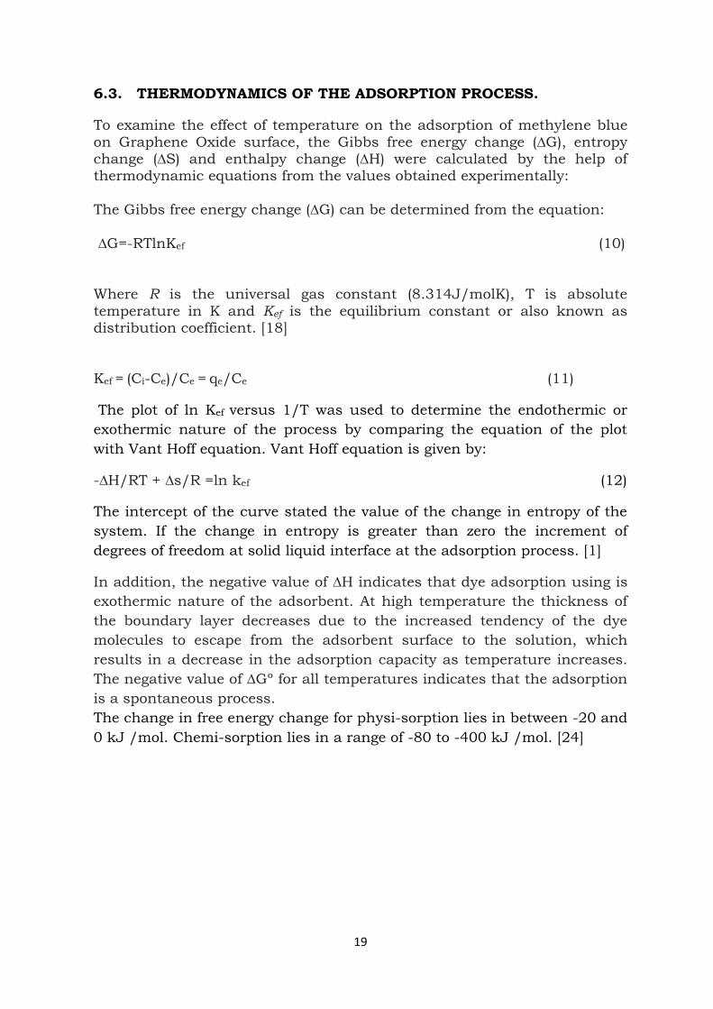
6.3. THERMODYNAMICS OF THE ADSORPTION PROCESS.

To examine the effect of temperature on the adsorption of methylene blue

on Graphene Oxide surface, the Gibbs free energy change (∆G), entropy change (∆S) and enthalpy change (∆H) were calculated by the help of thermodynamic equations from the values obtained experimentally:

The Gibbs free energy change (∆G) can be determined from the equation:

∆G=-RTlnKef (10)

Where R is the universal gas constant (8.314J/molK), T is absolute

temperature in K and Kef is the equilibrium constant or also known as distribution coefficient. [18]

Kef = (Ci-Ce)/Ce = qe/Ce (11)

The plot of ln Kef versus 1/T was used to determine the endothermic or

exothermic nature of the process by comparing the equation of the plot

with Vant Hoff equation. Vant Hoff equation is given by:

-∆H/RT + ∆s/R =ln kef (12)

The intercept of the curve stated the value of the change in entropy of the

system. If the change in entropy is greater than zero the increment of

degrees of freedom at solid liquid interface at the adsorption process. [1]

In addition, the negative value of ∆H indicates that dye adsorption using is

exothermic nature of the adsorbent. At high temperature the thickness of

the boundary layer decreases due to the increased tendency of the dye

molecules to escape from the adsorbent surface to the solution, which

results in a decrease in the adsorption capacity as temperature increases.

The negative value of ∆Gº for all temperatures indicates that the adsorption

is a spontaneous process.

The change in free energy change for physi-sorption lies in between -20 and

0 kJ /mol. Chemi-sorption lies in a range of -80 to -400 kJ /mol. [24]

20

7. CHARACTERIZATION OF GRAPHENE AND GRAPHENE OXIDE

NANO SHEET

7.1. FTIR (Fourier Transform of infrared spectroscopy)

FTIR spectrum was done to confirm the successful oxidation of Graphite

powder to Graphene oxide and Graphene. The presence of different

functional groups of oxygen was confirmed in Graphene and Graphene

oxide. The presence of different types of oxygen functionalities in graphene

were confirmed at broad and wide peak at 2280 cm-1 can be attributed to

the O-H stretching vibrations of the C-OH groups and water.

(Venkateswara Rao K., et al.) The band located at 1710-1720cm-1 has been

assigned to stretching vibration of carboxyl groups on the edges of the layer

planes. (C.Hontoria Lucas et.al.)

Thus FTIR confirmed the presence of hydroxyl group in Graphene and

Graphene oxide. Results obtained using this technique have allowed us to

establish some hypotheses about the type of surface oxygen groups present

in the graphite oxides, but they cannot conclusively establish their

chemical structures.

Figure showing FTIR spectra of G and Graphene oxide before adsorption.

4000 3500 3000 2500 2000 1500 1000 500

0

20

40

60

80

100

% T

Wavenumber (cm-1)

Graphene

Graphene oxide

21

7.2. SEM (SCANNING ELECTRON MICROSCOPE)

The SEM micrographs of synthesized GO with different scale bars are given

from the figure, it can be observed that Graphene oxide has layered

structure, which affords ultrathin and homogeneous Graphene films. Such

films are folded or continuous at times and it is possible to distinguish the

edges of individual sheets, including kinked and wrinkled areas. Graphene

and Graphene oxide both from layered structure, irregular and folding as

shown in the images below.

Figure shows SEM micro graphs of Graphene

Figure below shows SEM micrographs of Graphene Oxide

22

8. METHYLENE BLUE REMOVAL FROM WATER USING THE METHOD

OFADSORPTION- A BATCH STUDY

8.1. PREPARATION OF STANDARD STOCK SOLUTION OF

METHYLENE BLUE

A standard stock solution of methylene blue having concentration of 500

mg/L was prepared by taking 500 mg of methylene blue in 1L of distilled

water. The dye was mixed thoroughly with the help of a magnetic stirrer.

After that the solution was stored. From the 500 mg/L solution different

concentration of solutions were prepared by dilution and were kept in

different test tubes.

After dilution, the samples in the test tube were taken and absorbance of

each samples were measured by using UV-spectrophotometer. The

wavelength at which the absorbance was measured is 667nm which is

specific for Methylene Blue. Water was used as a reference solution and

with respect to water the absorbance of each sample was measured.

After getting the absorbance of each solution, a standard curve was plotted

between absorbance Vs concentration. The data and the chart were very

essential because this graph would be used to get unknown concentration

values for known absorbance values which we will be obtaining further in

the experiment.

23

Table given below is showing different absorbance values for different

concentrations of methylene blue.

Concentration (mg/L) Absorbance 1 0.191

5 0.9061 10 1.8 25 2.671

50 8.3 100 16.1

150 29.1 200 38.3 250 53

300 68.2 350 73.1

400 81.4 450 85.1 500 100.7

The figure below is showing a plot of absorbance versus concentration.

y = 0.202xR² = 0.991

0

20

40

60

80

100

120

0 100 200 300 400 500 600

Ab

sorb

ance

A

concentration (mg/L)

absorbance

Linear (absorbance)

24

8.2. REMOVAL OF METHYLENE BLUE FROM WATER USING

GRAPHENE BY ADSORPTION

8.2.1. EFFECT OF OPERATING PARAMETERS ON THE ADSORPTION

OF METHYLENE BLUE:

The operating parameters such as effect of Temperature, pH, adsorbent

dosage and concentration of the adsorbate at different time intervals were

observed.

8.2.2. EFFECT OF VARIATION OF ADSORBENT DOSAGE ON

ADSORPTION:

Method: In four Borosil conical flasks of 250ml, 100 ml of working volume

of methylene blue solution were taken with an initial concentration of

Methylene Blue was 10 mg/L. To the solutions 0.025 gm, 0.050 gm, 0.075

gm and 0.1 gm of Graphene oxide were added respectively. Those solutions

were put into a shaker cum incubator at 150 rpm at 303K. The samples

were collected after different intervals of time i.e. 15 minutes, 30minutes,

45minutes, 60minutes, 120 minutes each and were centrifuged at 10,000

rpm for 12 minutes. The samples were then put under the UV spectro-

photometer and the absorbances were measured. From the absorbances

that were obtained, the concentrations were calculated from the standard

curve that was made before.

Table 1: Table below shows the final concentration obtained for methylene

blue after adsorption by different weights of the adsorbent at different time.

adsorbent

dosage (gm/0.1L of

Methylene Blue)

Initial

concentration

(mg/L)

concentration (mg/L)obtained at different

time intervals

15 min 30 min 45 min 60 min

120 min

0.025 10 6.99 5.39 4.81 3.66 2.02

0.050 10 6.74 5.02 3.85 2.62 0.76

0.075 10 4.56 4.06 2.78 1.74 0.64

0.100 10

2.83 1.42 1.24 0.74 0.59

25

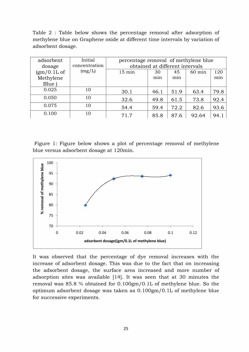
Table 2 : Table below shows the percentage removal after adsorption of

methylene blue on Graphene oxide at different time intervals by variation of

adsorbent dosage.

Figure 1: Figure below shows a plot of percentage removal of methylene

blue versus adsorbent dosage at 120min.

It was observed that the percentage of dye removal increases with the

increase of adsorbent dosage. This was due to the fact that on increasing

the adsorbent dosage, the surface area increased and more number of

adsorption sites was available [14]. It was seen that at 30 minutes the

removal was 85.8 % obtained for 0.100gm/0.1L of methylene blue. So the

optimum adsorbent dosage was taken as 0.100gm/0.1L of methylene blue

for successive experiments.

70

75

80

85

90

95

100

0 0.02 0.04 0.06 0.08 0.1 0.12

% r

em

ova

l of

me

thyl

en

e b

lue

adsorbent dosage((gm/0.1L of methylene blue)

adsorbent

dosage (gm/0.1L of

Methylene Blue )

Initial concentration

(mg/L)

percentage removal of methylene blue

obtained at different intervals

15 min 30 min

45 min

60 min 120 min

0.025 10 30.1 46.1 51.9 63.4 79.8 0.050 10 32.6 49.8 61.5 73.8 92.4 0.075 10 54.4 59.4 72.2 82.6 93.6 0.100 10 71.7 85.8 87.6 92.64 94.1

26

8.2.3. EFFECT OF VARIATION OF INITIAL pH ON ADSORPTION:

Method: The normal pH of methylene blue is 6.8. The initial pH of 10mg/L

of methylene blue was varied by using 0.1N HCl (to make it acidic) and

0.1N NaOH (to make it basic). The different pH of methylene blue was 2,

4,9,11 respectively. Each 0.1 L volume of working solution was transferred

in a 250ml Borosil flask and 0.1 gm of Graphene oxide was put into each

flask. The mixture was put into incubator cum shaker at 303K and

samples were collected at 15 minutes, 30minutes, 45 minutes, 60minutes,

and 120 minutes respectively. The samples were centrifuged at 10,000


photometer and the absorbances were measured. From those absorbances

which were obtained, the concentrations were calculated from the standard

curve that was made before. The values obtained from the experiment have

been given below.

Table 3: Table below shows concentration of methylene blue obtained after

adsorption by Graphene oxide at different interval of time and different pH.

Table 4: Table below shows percentage removal of methylene blue obtained

at different initial pH and at different time intervals.

pH of methylene

blue

solution

initial concentration of methylene

Blue (mg/L)

concentration (mg/L) of the adsorbent obtained at different intervals

15 min 30 min

45 min

60 min

120 min

2 10 7.202 7.143 6.108 6.094 3.089

4 10 6.212 4.143 2.123 1.064 1.049

9 10 0.133 0.094 0.074 0.069 0.064

11 10 0.074 0.069 0.049 0.0198 0.0049

pH of

methylene blue

solution

initial

concentration of methylene blue (mg/L)

percentage removal of the adsorbent obtained

after certain intervals

15 min 30

min

45

min

60 min 120

min

2 10 27.98 28.57 38.92 39.066 69.11

4 10 37.8 58.57 78.77 89.36 89.51

9 10 98.67 99.06 99.26 99.31 99.36

11 10 99.26 99.31 99.51 99.8 99.95

27

Figure 2: Figure below shows the percentage removal of methylene blue at

different pH and at 120minutes.

The percentage removal increased with increase in pH of the solution. This

happened because the pH of the solution had changed charge on the

surface of Graphene oxide. At lower pH two equilibriums existed.

The H+ ions compete with the cations of the dye at lower pH. Thus at lower

pH the adsorption was lower. At higher pH values more GO- ions occur

which enhances the electrostatic force of attraction and thus percentage

removal is more. [15]

Figure below shows the adsorption of methylene blue on Graphene oxide.

0

20

40

60

80

100

120

0 2 4 6 8 10 12

% r

em

ova

l of

me

thyl

en

e b

lue

pH

28

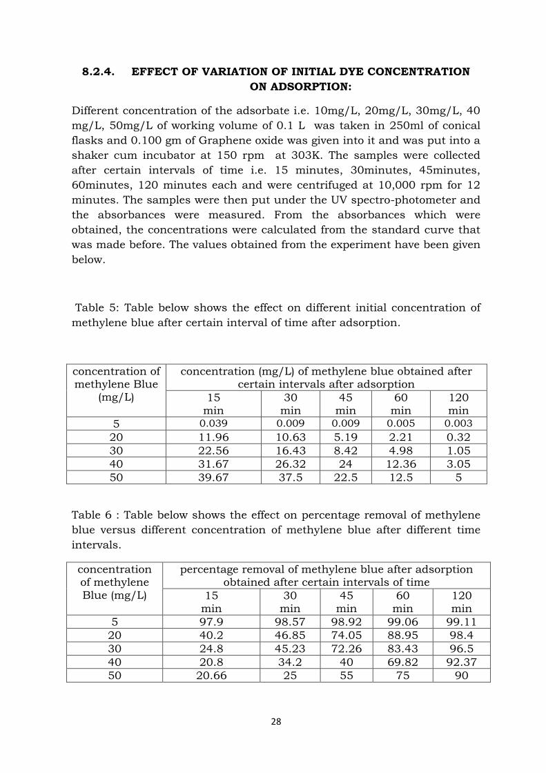
8.2.4. EFFECT OF VARIATION OF INITIAL DYE CONCENTRATION

ON ADSORPTION:

Different concentration of the adsorbate i.e. 10mg/L, 20mg/L, 30mg/L, 40

mg/L, 50mg/L of working volume of 0.1 L was taken in 250ml of conical

flasks and 0.100 gm of Graphene oxide was given into it and was put into a

shaker cum incubator at 150 rpm at 303K. The samples were collected

after certain intervals of time i.e. 15 minutes, 30minutes, 45minutes,

60minutes, 120 minutes each and were centrifuged at 10,000 rpm for 12

minutes. The samples were then put under the UV spectro-photometer and

the absorbances were measured. From the absorbances which were

obtained, the concentrations were calculated from the standard curve that

was made before. The values obtained from the experiment have been given

below.

Table 5: Table below shows the effect on different initial concentration of

methylene blue after certain interval of time after adsorption.

concentration of methylene Blue

(mg/L)

concentration (mg/L) of methylene blue obtained after certain intervals after adsorption

15 min

30 min

45 min

60 min

120 min

5 0.039 0.009 0.009 0.005 0.003

20 11.96 10.63 5.19 2.21 0.32

30 22.56 16.43 8.42 4.98 1.05

40 31.67 26.32 24 12.36 3.05

50 39.67 37.5 22.5 12.5 5

Table 6 : Table below shows the effect on percentage removal of methylene

blue versus different concentration of methylene blue after different time

intervals.

concentration of methylene

Blue (mg/L)

percentage removal of methylene blue after adsorption obtained after certain intervals of time

15 min

30 min

45 min

60 min

120 min

5 97.9 98.57 98.92 99.06 99.11

20 40.2 46.85 74.05 88.95 98.4

30 24.8 45.23 72.26 83.43 96.5

40 20.8 34.2 40 69.82 92.37

50 20.66 25 55 75 90

29

Figure: 3 The figure below shows the plot of percentage removal of

methylene blue versus different concentration of methylene blue obtained

after 120 minutes

Percentage removal decreased on increasing the temperature. There are

limited numbers of adsorbent sites present on the Graphene oxide which

becomes saturated after some time. Therefore at larger concentration most

of the molecules are left unadsorbed due to saturation of the binding sites.

[16]

8.2.5. EFFECT OF TEMPERATURE VARIATION ON ADSORPTION:

Into four 250ml conical flask, 0.1L working volume of methylene blue was

taken in each flask and 0.1gm of adsorbent was given in each flask and the

1st flask was placed at 313K, second flask at 308K, third flask at 298K and

the fourth one at 293K and each of the flask was shaken at 150 rpm. The

samples were collected from each flask after certain intervals of time i.e. 15

minutes 30minutes, 45minutes, 60minutes, and 120 minutes each and

were centrifuged at 10,000 rpm for 12 minutes. The samples were then put

under the UV spectro-photometer and the absorbances were measured.

From the absorbances obtained, the concentrations were calculated from

the standard curve that was made before. The values obtained from the

experiment have been given below.

88

90

92

94

96

98

100

0 10 20 30 40 50 60

% r

em

ova

l of

me

thyl

en

e lu

e

initial concentration of methylene blue (mg/L)

30

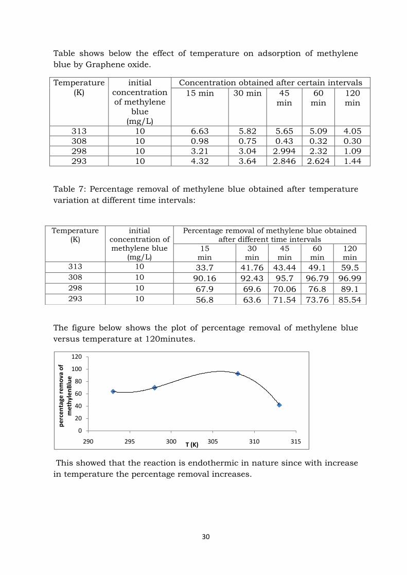
Table shows below the effect of temperature on adsorption of methylene

blue by Graphene oxide.

Temperature

(K)

initial

concentration of methylene

blue (mg/L)

Concentration obtained after certain intervals

15 min 30 min 45

min

60

min

120

min

313 10 6.63 5.82 5.65 5.09 4.05

308 10 0.98 0.75 0.43 0.32 0.30

298 10 3.21 3.04 2.994 2.32 1.09

293 10 4.32 3.64 2.846 2.624 1.44

Table 7: Percentage removal of methylene blue obtained after temperature

variation at different time intervals:

The figure below shows the plot of percentage removal of methylene blue

versus temperature at 120minutes.

This showed that the reaction is endothermic in nature since with increase

in temperature the percentage removal increases.

0

20

40

60

80

100

120

290 295 300 305 310 315

pe

rce

nta

ge r

em

ova

of

me

thyl

en

Blu

e

T (K)

Temperature (K)

initial concentration of methylene blue

(mg/L)

Percentage removal of methylene blue obtained after different time intervals

15 min

30 min

45 min

60 min

120 min

313 10 33.7 41.76 43.44 49.1 59.5 308 10 90.16 92.43 95.7 96.79 96.99 298 10 67.9 69.6 70.06 76.8 89.1 293 10 56.8 63.6 71.54 73.76 85.54

31

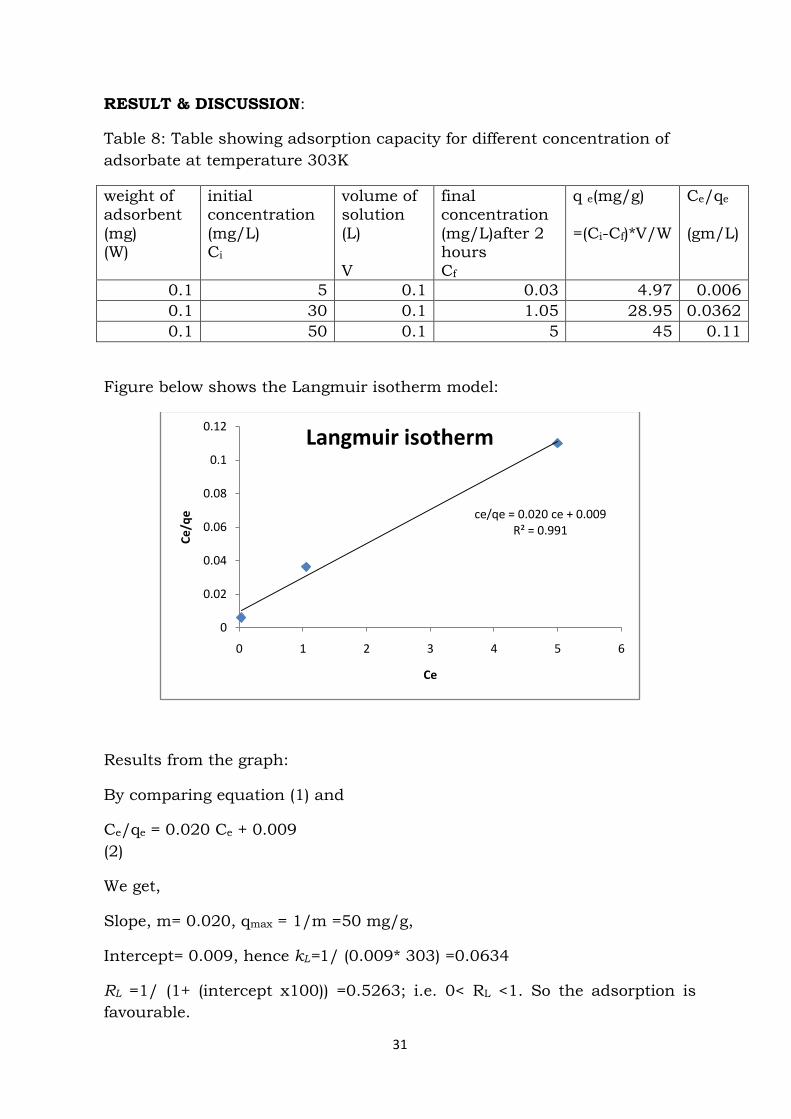
RESULT & DISCUSSION:

Table 8: Table showing adsorption capacity for different concentration of

adsorbate at temperature 303K

weight of adsorbent

(mg) (W)

initial concentration

(mg/L) Ci

volume of solution

(L) V

final concentration

(mg/L)after 2 hours Cf

q e(mg/g)

=(Ci-Cf)*V/W

Ce/qe

(gm/L)

0.1 5 0.1 0.03 4.97 0.006

0.1 30 0.1 1.05 28.95 0.0362

0.1 50 0.1 5 45 0.11

Figure below shows the Langmuir isotherm model:

Results from the graph:

By comparing equation (1) and

Ce/qe = 0.020 Ce + 0.009

(2)

We get,

Slope, m= 0.020, qmax = 1/m =50 mg/g,

Intercept= 0.009, hence kL=1/ (0.009* 303) =0.0634

RL =1/ (1+ (intercept x100)) =0.5263; i.e. 0< RL <1. So the adsorption is

favourable.

ce/qe = 0.020 ce + 0.009R² = 0.991

0

0.02

0.04

0.06

0.08

0.1

0.12

0 1 2 3 4 5 6

Ce

/qe

Ce

Langmuir isotherm

32

FREUNDLICH ISOTHERM:

Table 9: Table below shows adsorption capacity for different adsorbate

concentration at 303K

The figure below shows the freundlich isotherm

From graph slope, m=0.274 and intercept, c=3.340

By comparing equation (3) and

ln qe = 0.274 ln Ce + 3.340

We get, Kf= exp( 3.30)=27.11,

1/n=0.274, n=3.64

ln qe = 0.274ln ce + 3.340R² = 0.978

3.3

3.35

3.4

3.45

3.5

3.55

3.6

3.65

3.7

3.75

3.8

3.85

0 0.5 1 1.5 2

ln q

e

ln ce

Freundlich

weight of adsorbent

(mg) (W)


(mg/L) Ci

vol of sol

(L) V

final concentration

(mg/L)after 2 hours Cf

q e(mg/g) = (CiCf)*V/W

Ce/qe

gm/L

ln Ce ln qe

0.1 30 0.1 1.05 28.95 0.0362 0.048 3.36

0.1 40 0.1 3.052 36.95 0.0826 1.116 3.61

0.1 50 0.1 5 45 0.11 1.61 3.81

33

TEMKIN ISOTHERM MODEL:

Table 10: Table below shows adsorption capacity for different adsorbate

concentration at 303K

The figure below shows Temkin isotherm

Results from the graph:

From graph slope, m=9.837 and intercept, c=27.87

RT/b = B, B= 9.837, T=303K. R=8.314 (J/mol K)

RT ln(A/b)= 27.87

A= 258.936.

qe = 9.837(ln Ce) + 27.87R² = 0.956

0

5

10

15

20

25

30

35

40

45

50

0 0.5 1 1.5 2

qe

ln Ce

Temkin

weight of adsorbent

(mg) (W)


(mg/L) Ci

vol of sol (L)

V

final concentration (mg/L)after 2

hours Ce

q e(mg/g) =

(CiCf)*V/W

ln qe

0.1 30 0.1 1.05 28.95 3.36

0.1 40 0.1 3.052 36.95 3.61

0.1 50 0.1 5 45 3.81

34

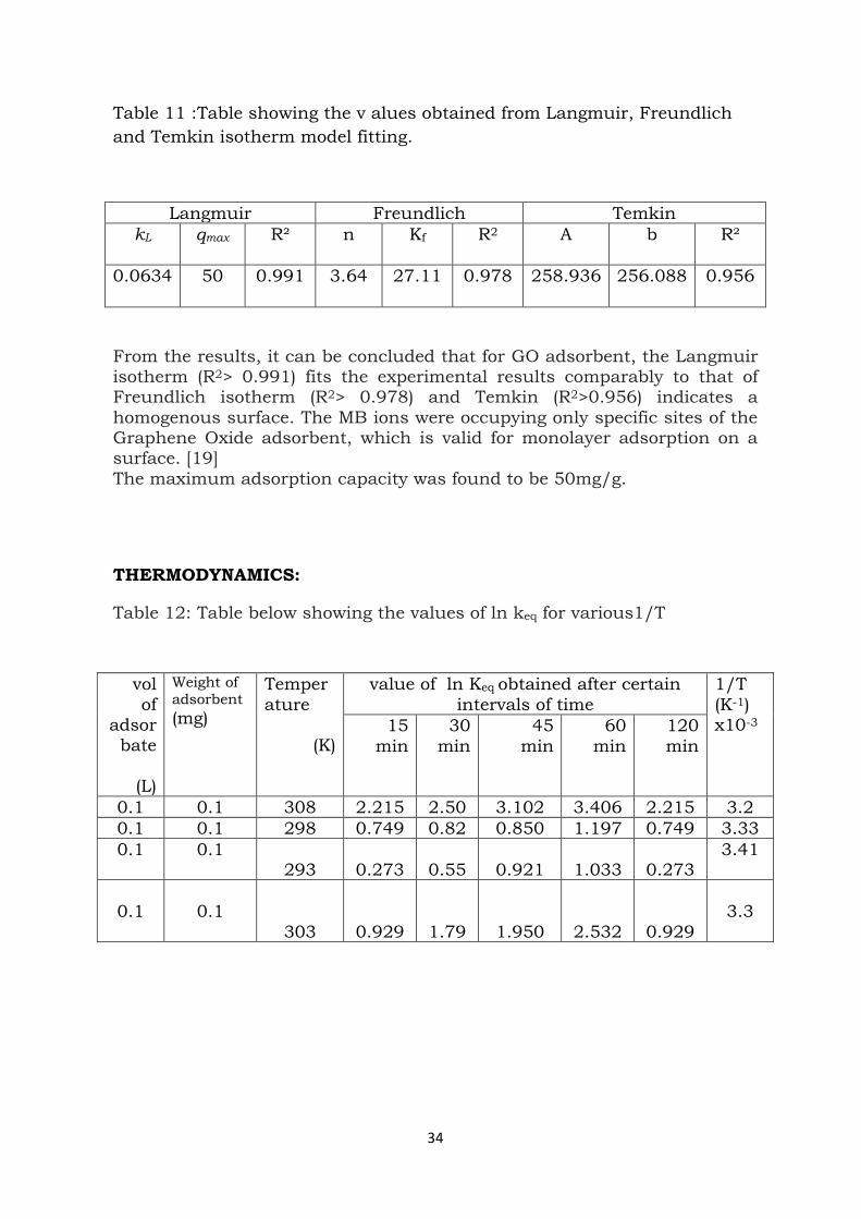
Table 11 :Table showing the v alues obtained from Langmuir, Freundlich

and Temkin isotherm model fitting.

Langmuir Freundlich Temkin

kL qmax R² n Kf R2 A b

R²

0.0634 50 0.991 3.64 27.11 0.978 258.936 256.088 0.956

From the results, it can be concluded that for GO adsorbent, the Langmuir isotherm (R2> 0.991) fits the experimental results comparably to that of Freundlich isotherm (R2> 0.978) and Temkin (R2>0.956) indicates a

homogenous surface. The MB ions were occupying only specific sites of the Graphene Oxide adsorbent, which is valid for monolayer adsorption on a surface. [19] The maximum adsorption capacity was found to be 50mg/g.

THERMODYNAMICS:

Table 12: Table below showing the values of ln keq for various1/T

vol

of adsorbate

(L)

Weight of

adsorbent

(mg)

Temper

ature

(K)

value of ln Keq obtained after certain

intervals of time

1/T

(K-1) x10-3 15

min

30

min

45

min

60

min

120

min

0.1 0.1 308 2.215 2.50 3.102 3.406 2.215 3.2

0.1 0.1 298 0.749 0.82 0.850 1.197 0.749 3.33

0.1 0.1 293 0.273 0.55 0.921 1.033 0.273

3.41

0.1

0.1

303 0.929 1.79 1.950 2.532 0.929

3.3

35

The figure below is showing the plot of ln keq versus 1/T

Table 13: Table below is showing the values ∆s and ∆H

Line no.

R2 equation time (hours) ∆s ∆H

1 0.926 ln keq =-15212T-1 + 52.68

1 52.68 -15212

2 0.860 ln keq = -13727T-1

+ 47.40 0.75 47.40 -13727

3. 0.956 ln keq = -12250T-1

+ 42.20 0.50 42.20 -12250

4. 0.865 ln keq= -10788T-1 +

36.95 0.25 36.95 -10788

It is seen from the graph and the table that the ∆s>0. This means that GO

has an affinity towards Methylene blue and ∆s varies between 36.95 J/mol

K to 52.68 KJ/mol K.

The values ∆s>0 indicated about the increment of degrees of freedom at

solid liquid interface at the adsorption process.

In addition, the negative value of ∆H indicates that dye adsorption using

GO is exothermic nature. At high temperature the thickness of the

boundary layer decreases due to the increased tendency of the dye

molecules to escape from the adsorbent surface to the solution, which

4. ln keq= -10788T-1 + 36.95R² = 0.865

3. ln keq = -12250T-1 + 42.20R² = 0.956

2. ln keq = -13727T-1 + 47.40R² = 0.860

1. ln keq = -15212T-1 + 52.68R² = 0.926

0

0.5

1

1.5

2

2.5

3

3.5

4

0.0032 0.00325 0.0033 0.00335 0.0034 0.00345

ln K

eq

T-1 (K-1)

Thermodynamics

1

2

4

3

36

results in a decrease in the adsorption capacity as temperature increases.

The value of ∆H varies in between -15212 J/mol and - 10788 J/mol.

To get the value of ∆G at a given temperature, we will have to consider

formula

∆G= -RTlnKef (7) Considering the values of 60minutes, we get the values of ∆G as follows:

Table14:

Temperatures

(K)

∆G (J/mol) ∆G

(KJ/mol)

303 -6378 -6.37

308 -8721.78 -8.721

298 -2965.65 -2.965

293 -2517.68 -2.517

The negative value of ∆Gº for all temperatures indicates that the adsorption

is a spontaneous process.

The change in free energy change for physi-sorption lies in between -20 and 0 kJ /mol. Chemisorptions lies in a range of -80 to -400 kJ /mol. Hence the values of ∆G lie in between -20KJ/mol and 0 KJ/mol hence the

type of adsorption is physi-sorption.

Table 15: Table below is showing the different values of adorption capacity

and its ratio at different time interval

ci mg/L

vol (L)

mass (gm)

cf

mg/L time hour

qt

mg/g t/q hour/(mg/g)

ln (qe-qt) t1/2

hour1/2

20 0.1 0.1 5.2 0.25 14.8 0.016 1.585 0.5

20 0.1 0.1 4.32 0.5 15.68 0.031 1.38 0.707

20 0.1 0.1 3.19 0.75 16.81 0.044 1.054 0.866

20 0.1 0.1 2.64 1 17.36 0.057 0.841 1

37

Figure below is representing pseudo first order model

Figure below is representing pseudo second order model

y = -1.025x + 1.857R² = 0.990

0

0.2

0.4

0.6

0.8

1

1.2

1.4

1.6

1.8

0 0.2 0.4 0.6 0.8 1 1.2

ln (

qe

-qt)

t(h)

pseudo 1st order

y = 0.047x + 0.007R² = 0.996

0

0.02

0.04

0.06

0.08

0.1

0.12

0 0.5 1 1.5 2 2.5

t/q

t (h)

pseudo second order

38

Figure below is showing intra particle diffusion model

The regression coefficient of pseudo second order was found to be more

than the other model. The regression coefficient is 0.996. Hence the

adsorption follows pseudo second order model.

discussions:

The adsorption follows Langmuir model. That is monolayer

adsorption takes place.

The adsorption follows pseudo second order kinetics.

The adsorption process is endothermic, spontaneous reaction.

y = 5.295x + 12.09R² = 0.988

14.5

15

15.5

16

16.5

17

17.5

18

0 0.2 0.4 0.6 0.8 1 1.2

qt

t1/2

intra particle diffusion

39

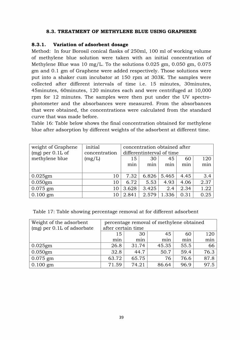
8.3. TREATMENT OF METHYLENE BLUE USING GRAPHENE

8.3.1. Variation of adsorbent dosage

Method: In four Borosil conical flasks of 250ml, 100 ml of working volume

of methylene blue solution were taken with an initial concentration of

Methylene Blue was 10 mg/L. To the solutions 0.025 gm, 0.050 gm, 0.075

gm and 0.1 gm of Graphene were added respectively. Those solutions were

put into a shaker cum incubator at 150 rpm at 303K. The samples were

collected after different intervals of time i.e. 15 minutes, 30minutes,

45minutes, 60minutes, 120 minutes each and were centrifuged at 10,000



that were obtained, the concentrations were calculated from the standard

curve that was made before.

Table 16: Table below shows the final concentration obtained for methylene

blue after adsorption by different weights of the adsorbent at different time.

weight of Graphene

(mg) per 0.1L of methylene blue

initial


concentration obtained after

differentinterval of time

15

min

30

min

45

min

60

min

120

min

0.025gm 10 7.32 6.826 5.465 4.45 3.4

0.050gm 10 6.72 5.53 4.93 4.06 2.37

0.075 gm 10 3.628 3.425 2.4 2.34 1.22

0.100 gm 10 2.841 2.579 1.336 0.31 0.25

Table 17: Table showing percentage removal at for different adsorbent

Weight of the adsorbent (mg) per 0.1L of adsorbate

percentage removal of methylene obtained after certain time

15 min

30 min

45 min

60 min

120 min

0.025gm 26.8 31.74 45.35 55.5 66

0.050gm 32.8 44.7 50.7 59.4 76.3

0.075 gm 63.72 65.75 76 76.6 87.8

0.100 gm 71.59 74.21 86.64 96.9 97.5

40

Table showing percentage removal of methylene blue, at different interval of

time, for different weights of adsorbent.

It was observed that the percentage of dye removal increases with the increase of adsorbent dosage. This was due to the fact that on increasing

the adsorbent dosage, the surface area increased and more number of adsorption sites was available [14]. It was seen that at 30 minutes the

removal was 74.21 % obtained for 0.100gm/0.1L of methylene blue. So the optimum adsorbent dosage was taken as 0.100gm/0.1L of methylene blue for successive experiments.

8.3.2. EFFECT OF VARIATION OF INITIAL DYE CONCENTRATION

ON ADSORPTION:

Different concentration of the adsorbate i.e. 10mg/L, 20mg/L, 30mg/L, 40

mg/L, 50mg/L of working volume of 0.1 L was taken in 250ml of conical

flasks and 0.100 gm of Graphene was given into it and was put into a





the absorbances were measured. From the absorbances which were



below.

0

20

40

60

80

100

120

0 50 100 150

% r

em

ova

l of

me

thyl

en

e b

lue

time

0.025 gm

0.050 gm

0.075 gm

0.100 gm

41

Table 18: Table below shows the effect on different initial concentration of

methylene blue after certain interval of time after adsorption

Table 19: Table below shows the percentage removal of methylene blue

obtained different intervals of time

Concentration of methylene bluesolution (mg/L)

weight of adsorbent(mg)/0.1Lof adsorbate

concentration of methylene blue(mg/L) obtained at different intervals of time

15 min

30 min

45 min

60 min

120 min

10 0.100gm 2.84 2.57 1.33 0.31 0.25

20 0.100 gm 15.2 10.6

8

5.46 2.63 1.79

30 0.100 gm 26.4 19.6 11.6 9.64 4.86

40 0.100 gm 35.8 21.2 16.5 14.9 13.2

Concentration of methylene blue solution (mg/L)

percentage removal of methylene blue obtained at different intervals of time

15 min 30min 45 min 60 min 120 min

10 71.59 74.21 86.64 96.9 97.5

20 23.8 46.6 72.7 86.85 91.05

30 11.93 34.6 61.3 67.86 83.8

40 10.275 46.9 58.725 62.575 66.825

42

Figure below shows the percentage removal of methylene blue at different

temperature

Percentage removal decreased on increasing the concentration. There are




[16]

0102030405060708090

100110

0 20 40 60 80 100 120 140

per

cen

tage

rem

ova

l

time (min)

percentage removal Vs time

10 20 30

43

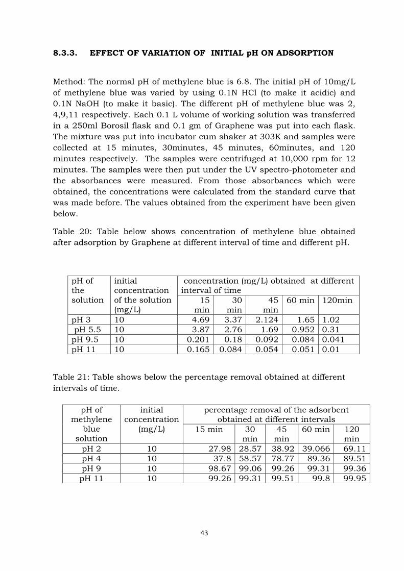
8.3.3. EFFECT OF VARIATION OF INITIAL pH ON ADSORPTION

Method: The normal pH of methylene blue is 6.8. The initial pH of 10mg/L

of methylene blue was varied by using 0.1N HCl (to make it acidic) and

0.1N NaOH (to make it basic). The different pH of methylene blue was 2,

4,9,11 respectively. Each 0.1 L volume of working solution was transferred

in a 250ml Borosil flask and 0.1 gm of Graphene was put into each flask.

The mixture was put into incubator cum shaker at 303K and samples were

collected at 15 minutes, 30minutes, 45 minutes, 60minutes, and 120

minutes respectively. The samples were centrifuged at 10,000 rpm for 12


the absorbances were measured. From those absorbances which were



below.

Table 20: Table below shows concentration of methylene blue obtained

after adsorption by Graphene at different interval of time and different pH.

Table 21: Table shows below the percentage removal obtained at different

intervals of time.

pH of the

solution


of the solution (mg/L)

concentration (mg/L) obtained at different interval of time

15 min

30 min

45 min

60 min 120min

pH 3 10 4.69 3.37 2.124 1.65 1.02

pH 5.5 10 3.87 2.76 1.69 0.952 0.31

pH 9.5 10 0.201 0.18 0.092 0.084 0.041

pH 11 10 0.165 0.084 0.054 0.051 0.01

pH of methylene

blue

solution


(mg/L)

percentage removal of the adsorbent obtained at different intervals

15 min 30 min

45 min

60 min 120 min

pH 2 10 27.98 28.57 38.92 39.066 69.11

pH 4 10 37.8 58.57 78.77 89.36 89.51

pH 9 10 98.67 99.06 99.26 99.31 99.36

pH 11 10 99.26 99.31 99.51 99.8 99.95

44

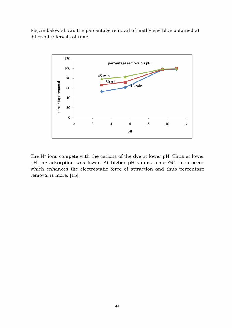
Figure below shows the percentage removal of methylene blue obtained at

different intervals of time

The H+ ions compete with the cations of the dye at lower pH. Thus at lower

pH the adsorption was lower. At higher pH values more GO- ions occur

which enhances the electrostatic force of attraction and thus percentage

removal is more. [15]

0

20

40

60

80

100

120

0 2 4 6 8 10 12

pe

rce

nta

ge r

em

ova

l

pH

percentage removal Vs pH

15 min

45 min

30 min

45

8.3.4. EFFECT OF VARIATION OF TEMPERATURE AT DIFFERENT

TEMPERATURES

Into four 250ml conical flask, 0.1L working volume of methylene blue

was taken in each flask and 0.1gm of adsorbent was given in each flask

and the 1st flask was placed at 313K, second flask at 308K, third flask

at 298K and the fourth one at 293K and each of the flask was shaken at

150 rpm. The samples were collected from each flask after certain

intervals of time i.e. 15 minutes 30minutes, 45minutes, 60minutes, and

120 minutes each and were centrifuged at 10,000 rpm for 12 minutes.

The samples were then put under the UV spectro-photometer and the

absorbances were measured. From the absorbances obtained, the

concentrations were calculated from the standard curve that was made

before. The values obtained from the experiment have been given below.

Table 22 : The table below shows concentration obtained for methylene

blue at different intervals of time

temperature

(K)

initial


Concentration(mg/L) obtained at


15min

30min

45min

60min

120min

308 10 0.784 0.499 0.26 0.241 0.22

303 10 2.841 2.579 1.336 0.31 0.25

298 10 3.86 2.97 2.61 1.76 1.09

293 10 4.21 3.56 2.98 2.01 1.56

Table 23: percentage removal of methylene blue obtained at different intervals of time

Temperature

(K)

initial

concentration (mg/L

percentage removal obtained after

certain interval of time

15 min

30 min

45 min

60 min

120 min

308 10 92.16 95.01 97.4 97.59 97.8

303 10 71.59 74.21 86.64 96.9 97.5

298 10 61.4 70.3 73.9 82.4 89.1

293 10 57.9 64.4 70.2 79.9 84.4

46

Figure below shows shows percentage removal obtained at 20° C and 30°C

The percentage removal increases on increase of temperature. This states

that the nature of the reaction is endothermic.

0

20

40

60

80

100

120

0 20 40 60 80 100 120 140

per

cen

tage

rem

ova

l

time (min)

percentage removal vs time at different temperature

30 degrees 20

47

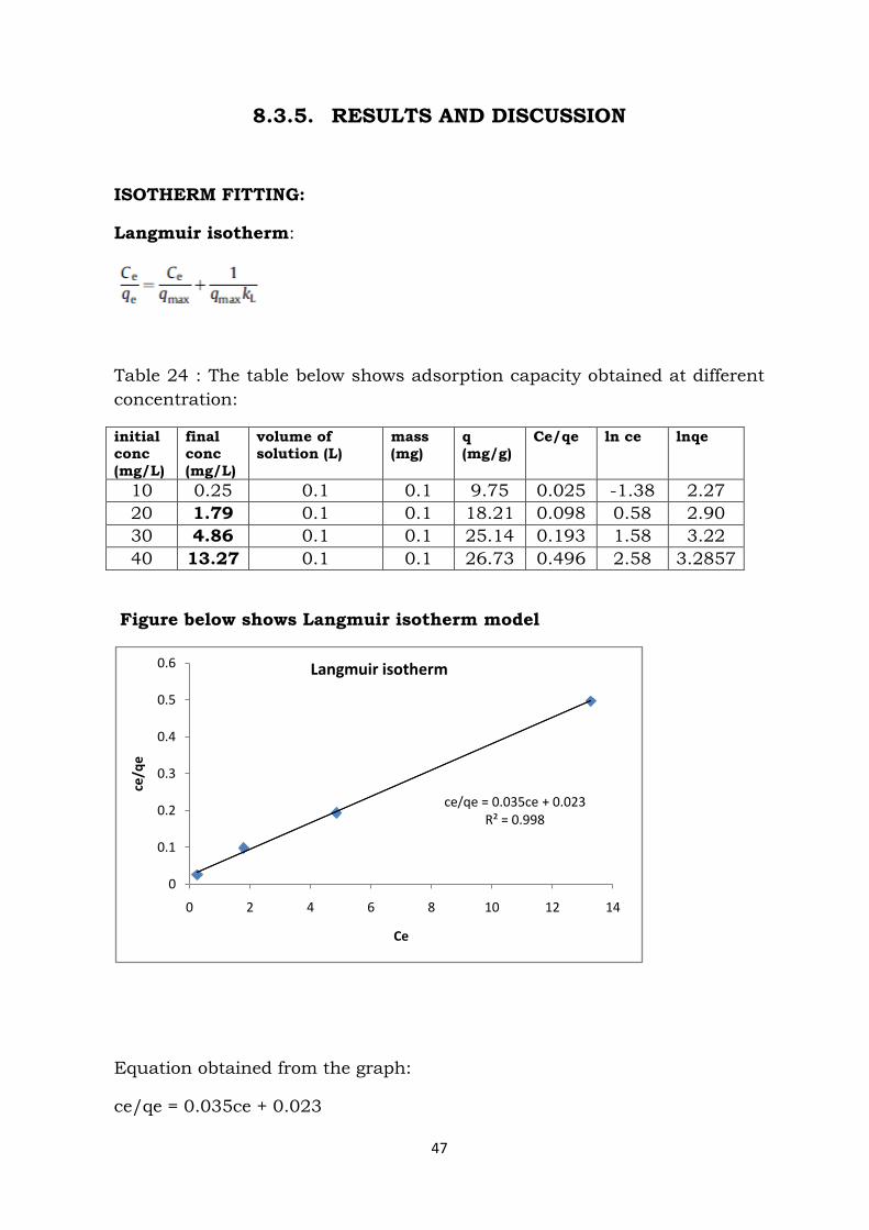
8.3.5. RESULTS AND DISCUSSION

ISOTHERM FITTING:

Langmuir isotherm:

Table 24 : The table below shows adsorption capacity obtained at different

concentration:

initial conc

(mg/L)

final conc

(mg/L)

volume of solution (L)

mass (mg)

q (mg/g)

Ce/qe ln ce lnqe

10 0.25 0.1 0.1 9.75 0.025 -1.38 2.27

20 1.79 0.1 0.1 18.21 0.098 0.58 2.90

30 4.86 0.1 0.1 25.14 0.193 1.58 3.22

40 13.27 0.1 0.1 26.73 0.496 2.58 3.2857

Figure below shows Langmuir isotherm model

Equation obtained from the graph:

ce/qe = 0.035ce + 0.023

ce/qe = 0.035ce + 0.023R² = 0.998

0

0.1

0.2

0.3

0.4

0.5

0.6

0 2 4 6 8 10 12 14

ce/q

e

Ce

Langmuir isotherm

48

qmax= 1/0.035 =28.57 mg/g (maximum adsorption capacity)

kL = 1/(28.57 x0.035)= 0.999, (0<KL <1) ( favourable)

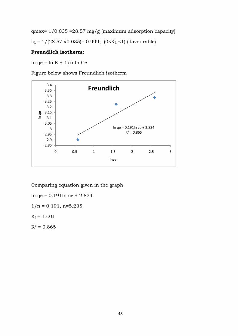
Freundlich isotherm:

ln qe = ln Kf+ 1/n ln Ce

Figure below shows Freundlich isotherm

Comparing equation given in the graph

ln qe = 0.191ln ce + 2.834

1/n = 0.191, n=5.235.

Kf = 17.01

R² = 0.865

ln qe = 0.191ln ce + 2.834R² = 0.865

2.85

2.9

2.95

3

3.05

3.1

3.15

3.2

3.25

3.3

3.35

3.4

0 0.5 1 1.5 2 2.5 3

ln q

e

lnce

Freundlich

49

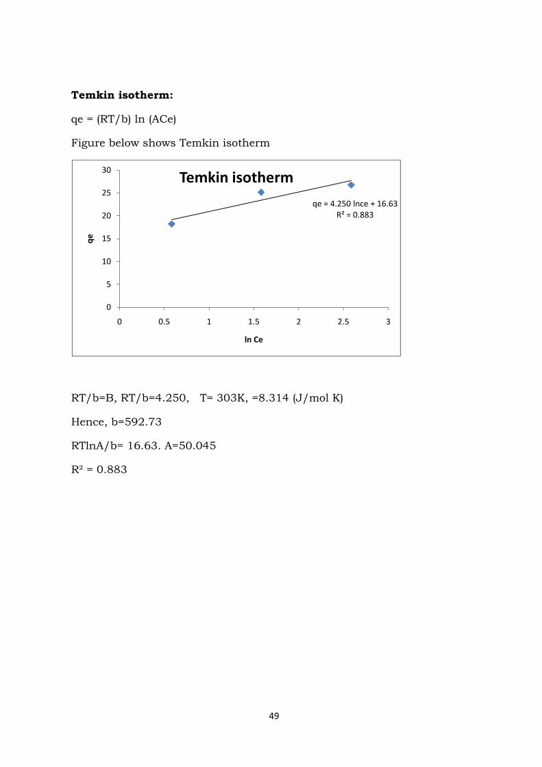
Temkin isotherm:

qe = (RT/b) ln (ACe)

Figure below shows Temkin isotherm

RT/b=B, RT/b=4.250, T= 303K, =8.314 (J/mol K)

Hence, b=592.73

RTlnA/b= 16.63. A=50.045

R² = 0.883

qe = 4.250 lnce + 16.63R² = 0.883

0

5

10

15

20

25

30

0 0.5 1 1.5 2 2.5 3

qe

ln Ce

Temkin isotherm

50

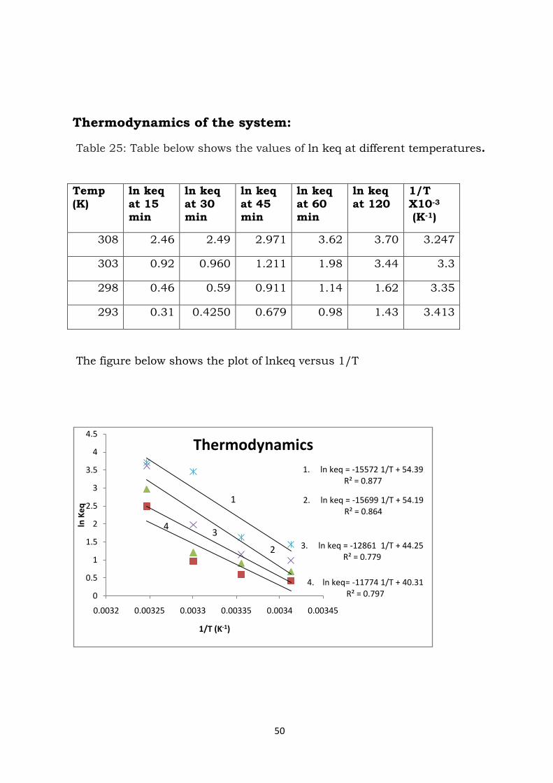
Thermodynamics of the system:

Table 25: Table below shows the values of ln keq at different temperatures.

Temp

(K)

ln keq

at 15 min

ln keq

at 30 min

ln keq

at 45 min

ln keq

at 60 min

ln keq

at 120

1/T

X10-3 (K-1)

308 2.46 2.49 2.971 3.62 3.70 3.247

303 0.92 0.960 1.211 1.98 3.44 3.3

298 0.46 0.59 0.911 1.14 1.62 3.35

293 0.31 0.4250 0.679 0.98 1.43 3.413

The figure below shows the plot of lnkeq versus 1/T

4. ln keq= -11774 1/T + 40.31R² = 0.797

3. ln keq = -12861 1/T + 44.25R² = 0.779

2. ln keq = -15699 1/T + 54.19R² = 0.864

1. ln keq = -15572 1/T + 54.39R² = 0.877

0

0.5

1

1.5

2

2.5

3

3.5

4

4.5

0.0032 0.00325 0.0033 0.00335 0.0034 0.00345

ln K

eq

1/T (K-1)

Thermodynamics

1

2

34

51

Let us consider equation 1 from the graph:

ln keq = -15572 1/T + 54.39

And comparing with equation

Where, R is the universal gas constant = (8.314 J/mol K), T in K

-∆H/R= -15572

Or ∆H = 15572 kJ/ mol. (Endothermic reaction)

∆s = 54.39 (∆s >0) (affinity of graphene towards methylene blue).

Values of:

∆ G (308) =-RTlnK = -8.314x308x 2.464287= -6309.59J/ mol

∆ G (303) = -RTlnK = -8.314x303x 0.924214= -2366.64J/ mol ∆ G (298) = -RTlnK = -8.314x398x 0.464158= -1535.88J/ mol

It has been found that ∆G< 0 (spontaneous process).

52

Kinetics of the adsorption process

Table 26: Table below shows different values for determining the kinetic

model.

initial

con (mg/L)

final

con (mg/l)

vol

(L)

wt

(gm)

q

(mg/g)

time

(h)

t/q qe-qt ln (qe-

qt)

t 1/2

20 15.24 0.1 0.1 4.76 0.25 0.052 13.45

2.59 0.5

20 10.68 0.1 0.1 9.32 0.5 0.053 8.89 2.18 0.70

20 5.46 0.1 0.1 14.54 0.75 0.051 3.67 1.30 0.86

20 2.63 0.1 0.1 17.37 1 0.057 0.84 -0.17 1

20 1.79 0.1 0.1 18.21 2 0.109 0 1.4

Pseudo first order kinetic model:

ln(qe − qt ) = ln qe − k1t

Figure below shows pseudo first order model

Comparing with the equation that is obtained from the graph:

ln( qe-qt) = -2.597 t+ 3.326

we get,

ln qe=3.326

k1= -2.597

ln( qe-qt) = -2.597 t+ 3.326R² = 0.958

0

0.5

1

1.5

2

2.5

3

0 0.1 0.2 0.3 0.4 0.5 0.6 0.7 0.8

ln (

qe

-qt)

t (h)

pseudo- 1st order

53

Pseudo second order kinetic model:

The equation is given by:

Figure below shows pseudo second order kinetic model

Comparing with equation from the graph:

y = 0.048x + 0.012

1/qe= 0.048

1/k2qe2 =0.012

R2 =0.990.

y = 0.048x + 0.012R² = 0.990

0

0.02

0.04

0.06

0.08

0.1

0.12

0 0.5 1 1.5 2 2.5

t/q

t (h)

pseudo-2nd order

54

Intra particle diffusion model:

qt = kpt 1/2 + C

Figure below shows the intra particle diffusion model.

Comparing with equation we get,

Kp= 5.589

C= thickness of the boundary layer=10.59

R2= 0.690

y = 5.589x + 10.59R² = 0.690

0

2

4

6

8

10

12

14

16

18

20

0 0.2 0.4 0.6 0.8 1 1.2 1.4 1.6

qt

t 1/2


55

Discussion:

From the isotherm model fitting it can be found that the regression

coefficient of the Langmuir model was 0.998 which is near to unity.

And the regression coefficient was found higher than that of

Freundlich and Temkin‟s. So we conclude that methylene blue

adsorption on Graphene was higher and it followed Langmuir

isotherm model. The maximum mono layer adsorption capacity was

found to be 28.57 mg/gm of Graphene. The dimensionless constant

for Langmuir isotherm RL also stated that the value of RL lies between

0 and 1. So the process is favorable. [Y. Li et al. / Materials Research

Bulletin 47 (2012) 1898–1904].

The thermodynamics of the system was studied and it provided

information about the energy changes involved in the process of

adsorption. The effect of temperature was considered to study the

thermodynamics of the system. The feasibility of the adsorption

process was calculated by the equation:

Where, R is the universal gas constant=8.314J/mol k.

T is the temperature in K.

Kd is called the distribution coefficient.

∆G was found to be negative for each temperature and it was seen

that as the system reached to higher temperature, the negative value

of ∆G was found to be higher, indicating that the adsorption was

more spontaneous when it was conducted at higher temperature. The

positive value of ∆ H showed that the process is endothermic in

nature. [30]. It was also found that ∆s>0. This stated the degree of

randomness increased during adsorption of MB on Graphene.

For determining the kinetics of the adsorption system, we took three

models, basically pseudo first order, pseudo second order and intra

particle diffusion. Among the three models, the regression coefficient

for pseudo second order model is more (i.e.0.990) so it indicated the

adsorption system followed the pseudo second order kinetics.

56

9. TREATMENT OF PHENOL USING GRAPHENE OXIDE

9.1. PREPARATION OF STANDARD STOCK SOLUTION:

A standard stock solution of phenol having concentration of 25 mg/L was

prepared by taking 25 mg of phenol in 1L of distilled water. The phenol was

mixed thoroughly with the help of a stirrer. After that the solution was

stored. From the 25 mg/L solution different concentration of solutions were

prepared by dilution and were kept in different test tubes.

After dilution, the samples in the test tube were taken and absorbance of

each samples were measured by using UV-spectrophotometer. The

wavelength at which the absorbance was measured is 210nm which is

specific for phenol. Water was used as a reference solution and with

respect to water the absorbance of each sample was measured.

After getting the absorbances of each solution, a standard curve was

plotted between absorbance Vs concentration. The data and the chart were

very essential because this graph would be used to get unknown

concentration values for known absorbance values which we will be

obtaining further in the experiment.

Table below shows the absorbances obtained at different concentration

Concentration (mg/L) Absorbances

2 0.1304

5 0.2993

8 0.4596

10 0.6049

15 0.8751

20 1.203

25 1.49

57

Figure below shows the standard curve for phenol

9.2. VARIATION OF THE WEIGHT OF THE ADSORBENT

Different weights of the adsorbent was taken in 0.1 L of 20mg/L of phenol

solution in 250ml of conical flasks and was put into a shaker cum

incubator at 150 rpm at 303K and to it different weights of the adsorbent

was given.. The samples were collected after certain intervals of time i.e. 15

min, 30min, 45min, 60min, 120 min each and were centrifuged at 10,000

rpm for 12 minutes. The samples were then put under the

UVspectrophotometer and the absorbances were checked. From the

absorbances obtained, the concentrations were calculated from the

standard curve that was made before. The values obtained from the

experiment have been given below

y = 0.059xR² = 0.999

0

0.2

0.4

0.6

0.8

1

1.2

1.4

1.6

0 5 10 15 20 25 30

a

b

s

o

r

b

a

n

c

e

concentration

58

Table 27: Table for concentrations obtained at different adsorbent dosage

Table 28 : Percentage removal of phenol at different interval of time is

provided below:

Weight of GO (mg)/0.1L of phenol

final concentration of phenol (mg/L) obtained at different intervals of time

15 min 30 min 45 min 60 min 120 min

0.025 19.633 19.16 18.3 17.93 17.58

0.05 18.68 17.73 17.25 17 16.98

0.075 16.83 15.84 16.63 14.6 12

0.1 14.97 13.27 11.17 9.37 8.86

weight of GO gm/0.1L

of phenol

percentage removal obtained after different intervals of time

15 30 45 60 120

0.025 1.835 4.2 8.5 10.35 12.1

0.05 6.6 11.35 13.75 15 15.1

0.075 15.85 20.77 27 34.6 40

0.1 25.15 33.65 44.15 53.15 55.7

59

Figure below shows the percentage removal obtained at different intervals

of time

It was observed that the percentage of phenol removal increases with the

increase of adsorbent dosage. This was due to the fact that on increasing

the adsorbent dosage, the surface area increased and more number of

adsorption sites was available [14]. It was seen that at 120 minutes the

removal was 55.7 % obtained for 0.100gm/0.1L of methylene blue. So the

optimum adsorbent dosage was taken as 0.100gm/0.1L of methylene blue

for successive experiments.

9.3. VARIATION OF INITIAL pH OF THE ADSORBATE.

Method: The normal pH of phenol is 4.9. The initial pH of 20mg/L of phenol

was varied by using 0.1N HCl (to make it acidic) and 0.1N NaOH (to make it

basic). The different pH of phenol was made 3,6,10 respectively. Each 0.1 L

volume of working solution was transferred in a 250ml Borosil flask and

0.1 gm of Graphene oxide was put into each flask. The mixture was put

into incubator cum shaker at 303K and samples were collected at 15

minutes, 30minutes, 45 minutes, 60minutes, and 120 minutes

respectively. The samples were centrifuged at 10,000 rpm for 12 minutes.

The samples were then put under the UV spectro-photometer and the

absorbances were measured. From those absorbances which were



below.

0

10

20

30

40

50

60

0 50 100 150

pe

rce

nta

ge r

em

ova

l

time

0.025

0.05

0.075

60

Table 29: Table below shows different concentrations obtained at different

pH

Table 30: Table below shows the percentage removal obtained at different

pH.

Table 31: Figure below shows percentage removal obtained at different pH

0

10

20

30

40

50

60

70

0 2 4 6 8 10

pe

rce

nta

ge r

em

ova

l

pH

percentage removal Vs pH

15

30

45

60

120

pH of the solution

concentration(mg/L) of phenol obtained after certain interval time

15 min

30 min

45 min

60 min

120 min

3 16.61 14.81 14.14 12.76 10.87

6 15.6 15.15 13.96 11.22 7.39

10 18.88 18.31 18.05 17.79 16.89

pH of the

solution

percentage removal of phenol obtained after different time

intervals

15

min

30

min

45

min

60

min

120

min

3 16.95 25.95 29.3 36.5 45.68

6 22 30.2 33.6 43.9 63.055

9 5.88 8.42 9.75 11.05 15.3

61

The adsorption of phenol by graphene oxide by the variation of pH was

found decrease on increasing the pH of the solution. This is because the pH

influences on the surface charge of the graphene oxide and on the

dissociation of phenol. At lower pH the adsorption is higher. At higher pH

the phenol forms phenolate anions. These phenolate anions get repelled

from the surface of the graphene oxide due to electrostatic repulsion,

thereby lowering the value of adsorption of phenol. [31]

9.4. VARIATION OF THE CONCENTRATION OF THE ADSORBATE

Different concentration of the adsorbate i.e. 10mg/L, 15mg/L, 20mg/L,

25 mg/L of working volume of 0.1 L was taken in 250ml of conical flasks

and 0.100 gm of Graphene oxide was given into it and was put into a




minutes. The samples were then put under the UV spectro-photometer

and the absorbances were measured. From the absorbances which were


was made before. The values obtained from the experiment have been

given below.

Table 32: Table below shows different concentration obatained after


concentration of phenol

(mg/L)

concentration obtained for phenol at different interval of time(mg/L)

15min 30min 45 min 60 min 120 min

10 8.13 6.44 3.69 2.847 2.56

15 13.42 11.89 11.08 8.67 4.74

20 16.10 15.15 13.29 11.22 7.389

25 23.62 23.06 21.93 18.94 16.64

62

Table 33: Table below shows percentage removal obtained at different

interval of time

Figure showing percentage removal versus time at different concentration

Percentage removal decreased on increasing the concentration. There are




0

10

20

30

40

50

60

70

80

0 50 100 150

% r

em

ova

l of

ph

en

ol

time (min)

10 mg/L

15 mg/L

20 mg/L

25 gm/L

Concentration of phenol

(mg/L)

percentage removal of phenol obtained at different interval of time

15 min 30min 45min 60min 120min

10 18.7 35.6 63.1 71.6 74.441

15 10.53 20.73 26.13 42.2 55.06

20 19.49 24.25 33.6 43.9 63.1

25 5.52 12.27 12.28 26.04 33.42

63

9.5. VARIATION OF TEMPERATURE

Into four 250ml conical flask, 0.1L working volume of phenol was taken

in each flask and 0.1gm of adsorbent was given in each flask and those

flask were placed at 293K, 298K, 303K, 308K and each of the flask was

shaken at 150 rpm. The samples were collected from each flask after

certain intervals of time i.e. 15 minutes 30minutes, 45minutes,

60minutes, and 120 minutes each and were centrifuged at 10,000 rpm

for 12 minutes. The samples were then put under the UV spectro-


obtained, the concentrations were calculated from the standard curve

that was made before. The values obtained from the experiment have

been given below.

Table 34: Table below shows the concentrations obtained after different

interval of time

temperature

(K)

concentration (mg/L) of phenol obtain after different interval of

time

15min 30 min 45 min 60 min 120 min

293 18.16 16.61 14.4 12.97 12.06

298 16.5 14.92 12.54 10.52 9.9

303 14.97 13.27 11.17 9.37 8.86

308 19.36 18.08 15.97 14.1 13.54

Table 35: Percentage removal obtained at different interval of time

temperature (K)

percentage removal of phenol obtained after different interval of time

15 min 30min 45min 60min 120 min

293 9.2 16.95 27.98 35.3 39.7

298 17.47 25.4 37.3 47.4 50.5

303 25.15 33.65 44.15 53.15 55.7

308 3.2 9.6 20.15 29.5 32.3

64

Percentage removal obtained after different interval of time

The percentage removal had increased with increase in temperature. This

showed that the process of adsorption is an endothermic process.

0

10

20

30

40

50

60

0 20 40 60 80 100 120 140

pe

rce

nta

ge r

em

ova

l of

ph

en

ol

time

20

25

30

35

65

9.6. RESULTS AND DISCUSSION:

Isotherm fitting:

Table 36: Table showing different values for fitting into different models

obtained from variation of concentration

Langmuir model :

Figure showing lang muir isotherm

initial

concentration

(mg/L)

final

concentration

(mg/L)

volume (mL)

mass of adsorbent

(mg)

qe ce/qe ln qe ln ce

10 2.56 0.1 0.1

8.44 0.18

2.13

2

0.4

4

15 4.74 0.1 0.1

8.26

0.81

5 2.11

1.9

0

20 7.38 0.1 0.1 12.6

1 0.58 2.53

1.9

9

25 16.64 0.1 0.1

8.36 1.99 2.12

2.8

1

y = 0.05x + 0.219R² = 0.998

0

0.1

0.2

0.3

0.4

0.5

0.6

0.7

0 1 2 3 4 5 6 7 8

ce/q

e

ce

Langmuir

66

From the graph we obtain, qmax= 1/0.05=20mg/gm

KL=0.228

RL= 1/(1+KL*100) =0.042, i,e. 0<RL<1 (favourable)

Freundlich model :

ln qe = ln Kf+ 1/n ln Ce

figure showing Frundlich isotherm

Comparing with equation of the graph:

1/n=0.499 or n=2.00

ln kf =1.51 or Kf =4.52

T (K)= 303K

y = 0.499x + 1.541R² = 0.999

0

0.5

1

1.5

2

2.5

3

0 0.5 1 1.5 2 2.5

lnq

e

ln Ce

Freundlich

67

Temkin model :

qe = (RT/b) ln (ACe)

Figure below shows Temkin isotherm

Chemical kinetics:

Table 37: Table showing the concentration values at different time intervals

time (hour)

ci (mg/L)

ce (mg/L)

volume L

weight (gm)

qt

(mg/g) t/q qe-qt ln (qe-

qt) t1/2

0.25 10 8.13 0.1 0.1 1.87 0.13 5.57 1.717 0.5

0.5 10 6.44 0.1 0.1 3.56 0.14 3.88 1.355 0.70

0.075 10 3.69 0.1 0.1 6.31 0.011 1.13 0.12 0.273

1 10 2.847 0.1 0.1 7.153 0.13 0.287 -1.24 1

2 10 2.56 0.1 0.1 7.44 0.26 0

y = 1.464x + 7.649R² = 0.268

0

2

4

6

8

10

12

14

0 0.5 1 1.5 2 2.5

qe

ln Ce

Temkin

68

Figure below shows pseudo first order model

Figure below shows pseudo second order model

y = -3.190x + 2.660R² = 0.909

0

0.2

0.4

0.6

0.8

1

1.2

1.4

1.6

1.8

2

0 0.1 0.2 0.3 0.4 0.5 0.6 0.7 0.8

ln (

qe

-qt)

time

pseudo first order

y = 0.080x + 0.107R² = 0.992

0

0.05

0.1

0.15

0.2

0.25

0.3

0 0.5 1 1.5 2 2.5

t/q

t

pseudo second order

69

Figure below shows intra particle diffusion model

It was found that the regression coefficient of pseudo second order

model is greater. Hence it can be concluded that adsorption of phenol

undergoes pseudo second order model.

Discussion:

The adsorption of phenol on graphene is a monolayer adsorption. It

follows Langmuir isotherm.

The adsorption of phenol by graphene oxide by the variation of pH

was found decrease on increasing the pH of the solution. This is

because the pH influences on the surface charge of the graphene

oxide and on the dissociation of phenol. At lower pH the adsorption is

higher. At higher pH the phenol forms phenolate anions. These

phenolate anions get repelled from the surface of the graphene oxide

due to electrostatic repulsion. Thus lowering the adsorption value.

The percentage removal increases on increasing the concentration of

the graphene oxide. This happened because on increasing the dosage

the surface area increases and the number of adsorption sites

increases.

The adsorption follows second order kinetics.

The percentage removal of phenol increases on increasing of

temperature this indicates that the nature of the adsorption id

endothermic.

y = 11.18x - 3.872R² = 0.970

0

1

2

3

4

5

6

7

8

0 0.2 0.4 0.6 0.8 1 1.2

qt

t 1/2


70

10. REFERENCE:

1. Farghali ,A.A. ; Bahgat,M.; Rouby, W.M.A. El; Khedr M.H. ; Journal of

Alloys and Compounds; 555 (2013) ;193–200.

2. Fakhri ,Ali; Journal of Saudi Chemical Society (2013).

3. Zhu, Yanwu; Murali ,Shanthi ; Cai, Weiwei ; Li ,Xuesong ; Suk,Won, Ji;

Jeffrey, Potts, R.; Ruoff, S. Rodney; Adv. Mater. 2010; 22, 3906–3924.

4. Lucas Hontoria-C.; Peinado Lopez J. A.; Gonzalez Lopez de d- J.;

Cervantes Rojas- L. M.; Mart M. R. Aranda; Carbon Vol. 33, 1995; 11,

1585-1592;.

5. Allen ,J. Matthew ; Tung , C. Vincent; Kaner, B. Richard; Chem. Rev.

2010; 110, 132–145.

6. Jr. Hummers, Williams; Offeman, Richarde; Preparation Of Graphitic

Oxide; 1958.

7. Ghosh ,Anupama; Subrahmanyam, S. K.; Krishna, Sai, Katla; Datta

,Sudipta; Govindaraj, A.; Pati K.Swapan; Rao, R. N. C. ; J. Phys. Chem.

2008; 112, 15704–15707.

8. Stoller ,Meryl ,D.; Park, Sungjin; Zhu, Yanwu; An ,Jinho; Ruoff ,S.

Rodney; Nano Letters Vol. 8;2008; 10,3498-3502.

9. Zhang, Wenjie ; Zhou, Chunjiao; Zhou, Weichang ;Lei, Aihua; Zhang,

Qinglin ; Wan, Qiang ; Zou, Bingsuo Bull Environ Contam Toxicol

,2011; 87,86–90.

10. Bradder, Philip; King, Ling ,Sie; Wang, Shaobin; Liu , Shaomin; J.

Chem. Eng. Data, 2011; 56, 138–141.

11. Liu, Tonghao; Li, Yanhui; Du ,Qiuju;Sun, Jiankun; Jiao, Yuqin;

Yang, Guangming; Wang, Zonghua; Xia, Yanzhi; Zhang, Wei; Wang

,Kunlin; Zhu, Hongwei; Wu ,Dehai; Colloids and Surfaces B:

Biointerfaces 90 (2012) 197– 203.

12. Deng, H., Lu, J., Li, G., Zhang, G., Wang, X., 2011. Adsorption of

methylene blue on adsorbent materials produced from cotton stalk.

Chem. Eng. J. 172, 326–334.

13. Chen, L., Ramadan, A., Lv, L., Shao, W., Luo, F., Chen, J., 2011b.

Biosorption of methylene blue from aqueous solution using lawny grass

modified with citric acid. J. Chem. Eng. Data 56, 3392–3399.

14. N. Nasuha, B.H. Hameed, A.T. Mohd Din, J. Hazard. Mater. 175

(2010) 126–132.

15. Zhang, W., Zhou. Chunjiao , Zhou. Weichang , Lei .Aihua, Zhang.

Qinglin, Wan. Qiang , Zou. Bingsuo,. 2011. Fast and Considerable

Adsorption of Methylene Blue Dyeonto Graphene Oxide.

16. W.-T. Tsai, H.-R. Chen, J. Hazard. Mater. 175 (2010) 844–849.

17. Makrigianni,V.,Giannakas,A.,De l i g i annak i s ,Y . ,Kon s tan t i nou

, . I , Journal of Environmental Chemical Engineering 3(2015)574–582.

18. Chowdhury .S, Chakraborty.S, Saha P. Colloids and Surfaces B: Biointerfaces 84 (2011) 520–527.

71

19. Foo K.Y., Hameed B.H., Insights into the modeling of adsorption isotherm systems, Chem. Eng. J. 156 (2010) 2–10.

20. Singh et al. Hazard. Mater. 150 (2008) 626–641. 21. Knop et al. Phenolic Resins – Chemistry, Applications and

Performance, Springer-Verlag, 1985. 22. Kharub.M, Journal of Environmental Research and Development.

(2012) Vol6. No. 3A.

23. Weber.J, Singh et al. Hazard. Mater. 150 (2008) 626–641. 24. Knop et al. Phenolic Resins – Chemistry, Applications and

Performance, Springer-Verlag, 1985.

25. Kharub.M, Journal of Environmental Research and Development. (2012) Vol6. No. 3A.

26. Weber. Adsorption processes XXIVth International Congress of Pure and Applied Chemistry(2013)

27. M.J. Jaycock, G.D. Parfitt, Chemistry of Interfaces, E. Horwood, 1981

28. Adsorption processes XXIVth International Congress of Pure and Applied Chemistry(2013)

29. M.J. Jaycock, G.D. Parfitt, Chemistry of Interfaces, E. Horwood, 1981

30. Haochun Shi et al Ind. Eng. Chem. Res., 2014, 53 (3), pp 1108–1118].

31. Y. Li et al. / Materials Research Bulletin 47 (2012)1898–1904.

http://pubs.acs.org/action/doSearch?ContribStored=Shi%2C+H

72

11. NOMENCLATURE:

Ce equilibrium dye concentration in solution (mg L−1)

Ci initial dye concentration (mg L−1)

Ct dye concentration in the liquid phase at time t

(mg L−1)

∆G◦ Gibbs free energy change (kJ mol−1)

∆H◦ enthalpy of reaction (kJ mol−1)

Kef distribution coefficient for adsorption

KF Freundlich constant (mg g−1) (L g−1)1/n

KL Langmuir constant (L mg−1)

k rate constant

kp sorption rate constant (L mg−1 min−1)

ki intraparticle diffusion rate constant (mg g−1min−0.5)

k1 pseudo-first-order rate constant (min−1)

k2 pseudo-second-order rate constant (g mg−1 min−1)

w weight of adsorbent (g)

n Freundlich adsorption isotherm constant

qt equilibrium dye uptake per g of the adsorbent at time t (mg g−1)

qe equilibrium dye uptake per g of the adsorbents (mg g−1)

qm maximum biosorption capacity (mg g−1)

R universal gas constant (8.314 J mol−1K−1)

R2 correlation coefficient

∆S◦ entropy of reaction (J mol−1 K−1)

T temperature (K)

V volume of the solution (L)

treatment of organic waste water

Documents