treatment of nearly-singular problems with the x-fem

HAL Id: hal-01015607https://hal.archives-ouvertes.fr/hal-01015607

Submitted on 26 Jun 2014

HAL is a multi-disciplinary open accessarchive for the deposit and dissemination of sci-entific research documents, whether they are pub-lished or not. The documents may come fromteaching and research institutions in France orabroad, or from public or private research centers.

L’archive ouverte pluridisciplinaire HAL, estdestinée au dépôt et à la diffusion de documentsscientifiques de niveau recherche, publiés ou non,émanant des établissements d’enseignement et derecherche français ou étrangers, des laboratoirespublics ou privés.

Treatment of nearly-singular problems with the X-FEMGrégory Legrain, Nicolas Moës

To cite this version:Grégory Legrain, Nicolas Moës. Treatment of nearly-singular problems with the X-FEM. AdvancedModeling and Simulation in Engineering Sciences, SpringerOpen, 2014, pp.1-13. 10.1186/s40323-014-0013-5. hal-01015607

https://hal.archives-ouvertes.fr/hal-01015607

https://hal.archives-ouvertes.fr

Legrain and Moes

RESEARCH

Treatment of nearly-singular problems with theX-FEMGregory Legrain* and Nicolas Moes

*Correspondence:

[email protected]

LUNAM Universite, GeM, UMR

CNRS 6183, Ecole Centrale de

Nantes, 1 rue de la Noe, 44321

Nantes, France

Full list of author information is

available at the end of the article

Abstract

In this paper, the behaviour of non-conforming methods is studied in the case ofthe approximation of nearly singular solutions. Such solutions appear whenproblems involve singularities whose center are located outside (but close) of thedomain of interest. These solutions are common in industrial structures thatusually involve rounded re-entrant corners. If these structures are treated withnon-conforming finite element methods such as the X-FEM (without anyenrichment) or the Finite Cell, it is demonstrated that despite being regular, theconvergence of the approximation can be bounded to an algebraic rate thatdepends on the solution. Reasons for such behaviour are presented, and twocomplementary strategies are proposed and validated in order to recover optimalconvergence rates. The first strategy is based on a proper enrichment of theapproximation thanks to the X-FEM, while the second is based on a proper meshdesign that follows a geometric progression. Performances of these approaches arecompared both in 1D and 2D, and enable to recover optimal convergence rates.

Keywords: X-FEM; Non-conforming; p-fem; singularity; convergence

Industrial structures usually involve re-entrant corners with possibly small fillets.

Accurate stress analysis for such structures requires the proper treatment of these

geometrical features. The size of these fillets is highly dependent on the manufac-

turing process, and depending on the quantity of interest and the size of the fillets

with respect to global scale of the structure, it may be neglected in the definition

of the mathematical model which is used for the computation. The problem is that

such areas with high curvature necessitates the use of very small elements, unless

blending mapping [1] or Nurbs-Enhanced FEM [2, 3] are used. These very small

elements have a high impact of the computational cost of the analysis, so that these

geometrical features are usually discarded in the analysis and replaced by acute

corners. In this case, the numerical solution is not consistent anymore with the

mathematical model: the verification of the model is not possible anymore, espe-

cially if the quantity of interest are related to stresses or strains in the fillet’s area.

The use of non-conforming approaches such as the X-FEM [4] or fictitious domain

approaches [5] can be considered in order to solve this mesh-density issue. Indeed,

conforming meshing can be avoided, the price being paid in the integration pro-

cess. In addition, one has to take care of the correct geometrical description: for

example, the use of a level-set for representing the geometry won’t allow to obtain

an accurate geometry, unless a mesh with a density of the order of the curvature

radius is used. Otherwise, one has to consider “sub-grid” level-sets as advocated in

[6, 7, 8], a fine pixelized representation, as in [9], or the so called Nurbs-Enhanced

Legrain and Moes Page 2 of 26

X-FEM [10]. By means of these strategies, the size of the computational mesh does

not have to be related to the size of the geometrical features. The solution being

regular, optimal convergence rates are expected. However, albeit being regular, me-

chanical fields can be very rough in the fillet area. As highlighted in the following,

this quasi-singularity prevents an optimal convergence of the solution when using

non conforming ”engineering” meshes i.e. meshes with a moderate number of ele-

ments. The objective of this contribution concerns the quantification of strategies

for improving the convergence rate of low and high-order non-conforming finite el-

ement methods. Two paths can be followed: (i) using the partition of unity [11]

and enrich the finite element approximation with adapted functions ; or (ii) using

p-fem strategies that are based on non-conforming meshes with proper grading near

the singularities [1]. These two strategies are first motivated in a one-dimensional

settings, then validated and compared in a 2D setting.

This work is organized as follows: first, mechanical fields near fillets are presented,

and their nearly singular behaviour highlighted. In a second part, the eXtended

Finite Element Method is introduced together with some recent improvement in the

field of high-order approximations. Then, a 1D model problem is introduced in order

to highlight the influence of nearly singular fields on the convergence properties of

the finite element method. A close study in the error contribution of the elements

of the mesh enables us to propose strategies in order to improve the convergence.

These strategies are extended in the 2D setting, and validated by means of various

numerical examples. Finally, performances of these strategies are compared before

concluding.

1 Near-fillets mechanical fields

As stated in the introduction, the example of a traction-free blunt re-entrant corner

is considered as an examples of nearly-singular problem. The geometry of interest

is depicted in figure 1(a). The opening angle of the corner is denoted as 2α, the

fillet radius as ρ and the local coordinate system as (r, θ). For comparison purpose,

we shall also consider the same problem, but with an acute angle in figure 1(b). In

order to understand the behaviour of the numerical schemes in the presence of blunt

corners, the asymptotic mechanical fields near the apex of the corner are presented.

The domain is assumed infinite and subjected to a remote uniform tension σ0.

The solution in the case of a sharp notch has been derived by [12]. The closed-

form solution in case of a rounded notch has been presented recently by Lazzarin

and Tovo [13] and Filippi et al. [14] among others. The solution of the problem is

obtained by making use of Kolosov-Muskhelishvili’s potential. Both solutions are

presented, so that their specific features can be highlighted.

1.1 Sharp corner

Following the work of Williams [12], the expression of the stress fields near a

traction-free re-entrant corner is written as the sum of two modes that have a

different singularity, λ1 and λ2. These eigenvalues verify the following equations:

sin(λ1α) + λ1 sin(α) = 0 (1)

sin(λ2α)− λ2 sin(α) = 0 (2)


x

y

2α

r

θ

M

ρ

r0

x

y

2α

r

θ

M

(a) (b)

Figure 1 Semi-infinite notch: (a) rounded notch; (b) sharp notch

λ1 (resp. λ2) is related to a symmetric (resp. anti-symmetric) mode. The expression

of the asymptotic stress field is thus [15]:

σij(r, θ) = K∗

1rλ1−1f1

ij(α, θ) +K∗

2rλ2−1f2

ij(α, θ) (3)

Factors K∗

i are called notch stress intensity factors (N-SIFs), and functions fkij

have the following expression:

f1rr

f1θθ

f1rθ

=

1

λ1 + 1 + χb1(1− λ1)

(3− λ1) cos((1− λ1)θ)− χb1(1− λ1) cos((1 + λ1)θ)

(λ1 + 1) cos((1− λ1)θ) + χb1(1− λ1) cos((1 + λ1)θ)

(1− λ1) sin((1− λ1)θ) + χb1(1− λ1) sin((1 + λ1)θ)

(4)

and:

f2rr

f2θθ

f2rθ

=

1

λ2 + 1 + χb2(1− λ2)

(3− λ2) sin((1− λ2)θ)− χb1(1− λ2) sin((1 + λ2)θ)

(λ2 + 1) sin((1− λ2)θ) + χb1(1− λ2) sin((1 + λ2)θ)

(1− λ2) cos((1− λ2)θ) + χb1(1− λ2) cos((1 + λ2)θ)

(5)

where (and using the notation α = qπ):

χb1 = − sin((1− λ1)qπ/2)

sin((1 + λ1)qπ/2)(6)

χb2 = − sin((1− λ2)qπ/2)

sin((1 + λ2)qπ/2)(7)

It can be seen that both modes produce singular stresses at the apex of the corner

when λi < 1, which causes a loss of convergence for finite elements, as discussed

in sections 1.3 and 3.1. In particular, for 2α = π/2, one finds λ1 = 0.5448 and

λ2 = 0.9085: Mode I is more singular than mode II.


1.2 Rounded corner

The determination of the asymptotic stresses near a rounded corner has been stud-

ied by Creager and Paris [16], Glinka [17], Lazzarin and Tovo [13], and improved

recently by Filippi et al. [14]. The two last contributions are based on the use

of Kolosov-Muskhelishvili’s potentials together with an auxiliary system of curved

coordinates that mimics the rounded corner’s geometry. This conformal mapping

approximation of the rounded notch has an hyperbolic shape which will have to

be taken into account in the numerical examples (see figure 2). Following [14], the

Figure 2 Analytical (dashed blue) and real (solid red) geometries for various opening angles. Itcan be noted that the larger the angle, the better the approximation of the real geometry.

stress distribution near the rounded notch is seen to be:

σij(r, θ) = K∗

1rλ1−1

[

f1ij(α, θ) + g1ij(r, α, θ)

]

+K∗

2rλ2−1

[

f2ij(α, θ) + g2ij(r, α, θ)

]

(8)

It is important to note that functions fkij are the same as in the case of the sharp

corner. Nevertheless, the resulting stress field is not singular as the origin of the

frame is out of the domain (see figure 1(a)). The expression of functions gkij are the

following:

g1rrg1θθg1rθ

=

q(

rr0

)µ1−λ1

4(q − 1) [λ1 + 1 + χb1(1− λ1)]

χd1 [(3− µ1) cos((1− µ1)θ)]− χc1 cos((1 + µ1)θ)

χd1 [(µ1 + 1) cos((1− µ1)θ)] + χc1 cos((1 + µ1)θ)

χd1 [(1− µ1) sin((1− µ1)θ)] + χc1 sin((1 + µ1)θ)

(9)

and:

g2rrg2θθg2rθ

=

q(

rr0

)µ2−λ2

4(q − 1) [λ2 + 1 + χb2(1− λ2)]

χd2 [(3− µ2) sin((1− µ2)θ)]− χc2 sin((1 + µ2)θ)

χd2 [(µ2 + 1) sin((1− µ2)θ)] + χc2 sin((1 + µ2)θ)

χd2 [(1− µ2) cos((1− µ2)θ)] + χc2 cos((1 + µ2)θ)

(10)

Factors χc1, χc2, χd1 and χd2 are given in [14], and µ1 and µ2 are solutions of the

following non-linear equations:


1− q(1 + µ1)

q[3− λ1 − χb1(1− λ1)]− ǫ1

(1 + µ1) cos[

(1− µ1)qπ

2

]

+

[

(1− µ1)2 − 1 + µ1

q

]

[3− λ1 − χb1(1− λ1)]− (3− µ1)ǫ1

cos[

(1 + µ1)qπ

2

]

= 0

(11)

and:

[

q(1 + µ2)− 2

q

]

[λ2 − 1− χb2(1 + λ2)]− ǫ2

(1− µ2) cos[

qπ

2(1− µ2)

]

+

(µ2 − 1)

[

q(µ2 − 3)− 2

q

]

[λ2 − 1− χb2(1 + λ2)] + (1− µ2)ǫ2

cos[

qπ

2(1 + µ2)

]

(12)

where ǫ1 and ǫ2 are also given in [14]. All the coefficients presented before can

be evaluated from the knowledge of the geometry of the rounded corner (i.e. its

opening angle 2α and its radius of curvature ρ). Finally, it is possible to obtain

the displacement field associated with this asymptotic stress field, by means of the

constitutive law and proper integration.

The displacement field has the following form:

ur(r, θ) = us,1r (r, θ) + us,2

r (r, θ) + ub,1r (r, θ) + ub,2

r (r, θ)

uθ(r, θ) = us,1θ (r, θ) + us,2

θ (r, θ) + ub,1θ (r, θ) + ub,2

θ (r, θ)(13)

The explicit expression of functions us,ir and ub,i

r are given in appendix A, and a

sketch of the first mode displacement and strain are presented in figures 3 and 4

Figure 3 Displacement field associated to a blunt corner of radius 0.00625 subjected to a mode Iloading.


Figure 4 Strain field (Von-Mises norm) associated to a blunt corner of radius 0.00625 subjectedto a mode I loading.

1.3 Discussion

I order to discuss the expected behaviour of the asymptotic solution derived in the

previous section, let us consider the terminology coined in [1]. This classification,

based on the features of the analytical solution of a problem, enables to predict the

behaviour of the finite element method. Solutions can be separated in three classes

:

Category A If the solution is analytic everywhere in the domain (including boundaries);

Category B If the solution is analytic everywhere, except at a finite number of singular

points (and edges in 3D);

Category C If the solution does not belong to the previous categories (material interfaces

for example);

Practical problems usually belong to category B. Note however that the solution is

not necessarily singular near singular points: it depends on the eigenvalues of the

expansion of the solution. If the eigenvalues are strictly smaller than one, then the

solution is singular and the problem is said strongly in category B. Otherwise, it is

qualified as weakly in category B.

As stated in section 1.1, the stress field associated with the sharp corner eqn.(3)

is singular and problems involving these geometrical features belong strongly to

category B. In this case, the convergence of the finite element method is bounded

by the order of the singularity of the solution i.e. min(λ1, λ2). Note however that

if 2α ≥ π, then λi ≥ 1, and the problem becomes regular (weakly in category B).

The convergence is thus bounded by the polynomial order of the approximation (for

h finite elements). On the contrary, the stress field related to the rounded corner

eqn.(8) is regular, although it can be very rough if the radius of curvature ρ is

small. The problem is then always weakly in category B, but if ρ is small then it

tends to be strongly in category B. As the solution is regular, one would expect h

convergence rates associated with the order p of the polynomial approximation (i.e.

in O(hp) in the energy norm). This is the case asymptotically, but not necessary for

”engineering meshes” (meshes with a moderate number of elements), as illustrated

in section 3.


2 The eXtended Finite Element Method

In the following, the eXtended Finite Element Method (X-FEM) will be used for the

computations. The X-FEM [4] is an extension of the finite element method (FEM)

that was developed from the need to improve the FEM approach for problems

with complex geometrical features (cracks [4], material interfaces [18], free surfaces

[18, 19]). In contrast to classical finite elements, the X-FEM does not require the

mesh to conform the geometry. Instead, a regular mesh is constructed for the domain

of interest and the presence of internal boundaries is taken into account in the

formulation of the finite elements at the corresponding locations by means of the

partition of unity method [11]. The X-FEM approximation of the displacement field,

u, over an element Ωe is given by:

u(x)|Ωe=

n∑

α=1

Nα

uα +

ne∑

β=1

aαβ ϕβ(x)

(14)

where the approximation can be divided into a classical one that depends only

on the vectorial shape functions Nα(x)[1] and classical degrees of freedom (dofs

in the following) uα, and an enriched one that depends on enrichment functions

ϕβ(x) and enriched dofs aαβ . Those functions prevent poor rates of convergence due

to the non-conformity of the approximation or the singularity of the solution. The

additional degrees of freedom are only added at the nodes whose support is split

by the interface, which means that typically only a few of them are added. More

precisely, if an element is fully enriched, then this number of enriched dofs is equal

to n×ne. On the contrary, no enrichment is used in the case of a non-conforming ap-

proximation: the weak form is just integrated selectively in the domain. A level-set

representation of the geometry is typically used: in this case, the level-set is inter-

polated on the approximation mesh. This couples the geometrical representation to

the approximation [20], and prevents the use of higher order approximations due

to an insufficient geometrical accuracy. A so-called sub-grid level-set approach has

been proposed in [6, 7] in order to uncouple geometry and approximation, and thus

allow the use of high-order approximations. Alternatively, the use of the so-called

Nurbs-Enhanced X-FEM [10] allows to consider the exact geometrical representa-

tion independently of the approximation mesh, see figure 6 for a comparison of both

approaches. In this case, geometries such as the one depicted in figure 5 could be

represented using a mesh whose characteristic length is large with respect to the

geometrical details. However, the following question arise: what is the influence of

the size mismatch between the mesh and the geometrical details on the convergence

of the finite element approximation ?

In this contribution, both low and high-order X-FEM will be considered. The lat-

ter case makes sense, as one can deal with meshes composed of big elements with

simple shape. In this case, the enrichment scheme presented in (14) can lead to con-

ditioning issues when a so-called geometrical enrichment is used [21]. Geometrical

[1]In (14), the vectorial nature of the field is handled by the shape functions, and

not the dofs that are just coefficients. This notation facilitates the writing of the

discrete operators.


Figure 5 Geometrical details in an element.

Sub-GridNurbs-Enhanced

Figure 6 Left: Nurbs-Enhanced X-FEM (in red, a typical integration cell); Right: Sub-Gridlevel-set. Thick lines indicate elements boundaries, and thin lines integration cells boundaries.


enrichment states that the size of the enriched region remains unchanged during

refinement (it is also called ”fixed area” enrichment in [22]). It is not related to the

concept of ”geometric mesh” which is commonly used in the p-fem community. In

order to improve this issue, several strategies have been proposed [21, 23, 22, 24].

In this contribution, the strategy proposed by Duarte et al. [25] and further studied

in Chevaugeon et al. [26] is considered. It consists in using a vectorial enrichment,

rather than a scalar one as in eqn.(14):

u(x)|Ωe=

n∑

α=1

Nαuα +

n∑

α=1

Nα

ne∑

β=1

aαβ ϕβ(x)

(15)

in this expression, the first term corresponds to the classical finite element approx-

imation while the second one corresponds to the enrichment. It involves Nα, the

scalar shape function associated with the partition of unity, aαβ the scalar enriched

dof and ϕβ(x) the βest vectorial enrichment function. Note that the number of

vectorial shape functions n remains unchanged with respect to (14), and that the

number of scalar shape functions n is smaller than n. More precisely, in the case

where N and N share the same polynomial order, we have n = nd with d the spatial

dimension of the problem. It reflects the different nature of these shape functions

(vectorial and scalar). This difference has also an influence on the number of en-

riched dofs: it is reduced by a factor d if (15) is used (n×ne rather than n×ne). In

[26], the resulting conditioning number evolution was shown to increase in O(1/h2)

for a model problem, which is the same rate as classical linear finite elements. This

improvement in the conditioning number is of great interest in practice, as is allows

to use the so-called geometrical enrichment which has been proved to be optimal

in term of convergence. This aspect becomes fundamental when high-order shape

functions are used, as the conditioning number increases with the polynomial order.

3 1D model problem

The behaviour of the finite element approximation is studied on a simple 1D model

problem which is representative of the solution near the fillet:

d2u

dx2+ f = 0 x ∈]0, 1[ (16)

u(0) = u(1) = 0 (17)

f is chosen such that the exact solution is:

u0(x) = xα − x (18)

for α > 1/2. One can see that this solution is singular, and that the center of the

singularity is for x = 0. Such a solution can be compared to typical 2D solutions near

re-entrant corners: u = rβφ(θ) for α = β + 1/2. The problem is solved using h and

p finite element approximations, with both homogeneous or geometric meshes [27].

The finite element shape functions are based on integrated Legendre polynomials,

as presented in [1]. The problem is solved for x ∈ [ε, 1[, ε ∈ [0, 1[. Remark that a


conforming mesh is used for this simple problem: the conclusions can be extended

to the non-conforming case. We first consider the case where ε = 0: the singularity

emanates from the boundary of the domain. In the case of a quasi-uniform mesh,

the estimates given in [27] states that the energy norm of the error evolves as:

‖e‖E ≤ k N−β (19)

with β = min(p, α − 1/2) for h-refinement, and β = 2α − 1 for p-refinement. Note

that in both cases the convergence is algebraic, with an order which depends on the

singularity of the solution. In the case where the singularity lies out of the domain,

the convergence remains algebraic for h-refinement, whereas it becomes exponential

for p-refinement [28]:

‖e‖E ≤ k exp−γNθ

(20)

In this expression, k, γ and θ are positive constants that depend on the exact

solution.

3.1 Convergence for nearly singular problems

Equations (19) and (20) are checked on the model problem (16) with α = 0.55,

and for ε = 10−k, k ∈ [1, 2, 3, 4, 5]. Both h and p-convergence are considered, with a

regular nodal distribution. Note that all the figures in this section represent absolute

errors. The results are presented in figure 7 and 8: it can be seen that ε has a visible

effect on the behaviour of the two approaches. Large ε values correspond to very

smooth solutions in the domain, so that estimates (19) with β = p and (20) are

verified. On the contrary, small values for ε correspond to nearly-singular solutions

in spite of the absence of any singularity in the domain and on its boundary. The

convergence tends to be algebraic with a rate that depends on the singularity (α−1/2 for h-convergence, and 2α − 1 for p-convergence). In particular, two regimes

can be observed in figure 7: for low h the convergence is driven by the singularity

(β = α−0.5), whereas at some point the asymptotic β = p convergence is observed.

The smaller ε, the later this asymptotic convergence is recovered. Note that this

regular convergences can always be obtained, but not necessarily for “engineering”

meshes (i.e. with moderate element size). The reason for this loss of convergence

is now discussed more precisely in the p-Fem case: Consider the contribution of

the first four elements to the global error which is presented in figure 9(a) (for

α = 0.55, ε = 10−5 and 20 elements). It can be seen that only the first element has an

algebraic convergence, whereas the remaining elements converge exponentially. This

behaviour is typical of the singular case, where this phenomenon is well known. For

bigger ε, an exponential convergence is obtained for all the elements (see figure 9(b)).

Following [27] (in the case where ε = 0), the contribution η1 of the first element

(that touches the center of the singularity) to the error writes:

η1 ≃ C0(α)hα−1/21

p2α−1

(

1 +O( 1p ))

(p → ∞) (21)


1

1

Figure 7 Influence of the distance to the singularity, h-convergence

101 102 103

N dofs

10-11

10-10

10-9

10-8

10-7

10-6

10-5

10-4

10-3

10-2

10-1

100

Erro

r

p-FEM 20 elts ε=0.1p-FEM 20 elts ε=0.01p-FEM 20 elts ε=0.001p-FEM 20 elts ε=0.0001p-FEM 20 elts ε=1e-05

Figure 8 Influence of the distance to the singularity, p-convergence

101 102 103

N dofs

10-12

10-11

10-10

10-9

10-8

10-7

10-6

10-5

10-4

10-3

10-2

10-1

100

Erro

r

Total errorError element 0Error element 1Error element 2Error element 3

101 102 103

N dofs

10-12

10-11

10-10

10-9

10-8

10-7

10-6

10-5

10-4

10-3

10-2

10-1

100

Erro

r

Total errorError element 0Error element 1Error element 2Error element 3

(a) (b)

Figure 9 Contribution of the first elements to the global error: (a) ε = 10−5; (b) ε = 10

−2


Where h1 is the length of the element, and C0(α) is a constant. This shows that

the error decrease in the first element is algebraic. On the contrary, the estimate

for the remaining elements is:

ηi, i>1 ≃C1(α)hα−1/2i

(

1− r2i2ri

)α−1rpipα

(

1 +O( 1pσ )

)

(22)

ri =

√xi −

√xi−1√

xi +√xi+1

Where hi is the length of the element, C1(α) is a constant, and σ > 0. This equations

states that the convergence is exponential in all the elements but the first one. This

is why exponential convergence should be expected in the nearly-singular case, as

all the elements should follow estimate (22) (none of them touches the center of the

singularity). Although, figure 9(a) seems to contradict eqn.(22), this is not the case.

Indeed, eqn.(22) holds only if 0 < r2i < 1−1/p, which is not the case for figure 9(a),

as r2 ranges from 0.999 to 6.6 10−4 (see table 1). It can be seen that only the first

element has a r2 greater than 1 − 1/p ∀p, hence the algebraic convergence. When

1− 1/p < r2i < 1, following [28], the estimates becomes:

E(Ii) ≃ hα−1/2i

rp+1−αi

pα−1/2

(

1/pα−1/2 + (1− r2i )α−1/2

)

(23)

When r2i is close to 1, one obtain the same estimate as eqn.(21), which is consistent

with the numerical results (figure 9(a))[2].

Element r2

1 9.99 10−1

2 1.11 10−1

3 4.00 10−2

4 2.04 10−2

20 6.57 10−4

Table 1 Evolution of r2 for the elements of a regular mesh (ε = 10−5, 20 elements)

3.2 Strategies for recovering optimal convergence

Two strategies are proposed in order to recover a proper convergence in the case of

nearly-singular problems. The first one is based on an enrichment of the approxi-

mation, using the Partition of Unity method [11], see eqn.(14). The second one is

based on a proper mesh design, which is close to the approaches that are classically

used in the context of p-Fem.

Enrichment of the approximation

The idea consists in the enrichment of the approximation in order to capture the

steep gradients of the exact solution. The enrichment function considered is xα

as only this term is singular in (18), and a “geometrical” enrichment strategy is

considered, as it has been shown in practice that it was leading to better convergence

properties [21, 22]. Such an approach can be used for both h and p Fem.

[2]For ε = 10−2 (figure 9(b)), the maximum value of r2 is 0.51, which means that p

convergence is obtained for the first element for any p > 2.


Suitable mesh design

A second possibility, based on the construction of a suitable mesh is investigated

in the case when p-refinement is considered. It has been highlighted in the previous

section that in the case of p-Fem, the contribution of the first element was prevent-

ing any exponential convergence of the approximation. A sufficient condition for

recovering the exponential convergence consists in ensuring that this first element

converges exponentially. The objective is thus to prescribe r2 < 1 − 1p in the first

element. In the context of p-refinement, we have chosen to verify this condition for

small orders, i.e. p = 2. So, if r2 < 1/2 exponential convergence is expected for

all the elements and for any polynomial order greater than two. First, consider the

case of a regular mesh depicted in figure 10. We are interested in the first element

which is highlighted in red. This element is located at a distance ε from the center

of the singularity. For this first element, condition r2 < 1/2 can be written as:

(√ε+ h−√

ε√ε+ h+

√ε

)2

≤ 1

2(24)

Solving this equation for h gives the maximum length of the first element allowing

for an exponential convergence:

h ∈[

0, 4(

3√2 + 4

)

ε]

h ∈ [0, 33 ε](25)

Equation (25) states that in the case of a quasi-uniform mesh, the length of the

first elements must have the same order of magnitude as ε. This condition is very

restrictive in practice, as a quasi-uniform mesh of this type is unusable for real

problems. Note that the numerical results from figure 8 are consistent with this

estimate, as exponential convergence is noticeable for ε < 10−3 which is close to

h/33 ≃ 1.6 10−3.

0

x

1

ε h

Figure 10 Regular mesh with singularity out of the domain (x = 0). In red, the element ofinterest.

We now consider the use of a geometrical mesh. Indeed, it has been shown in the

case of singular problems [1] that the use of a finite element mesh with geometrical

progression of power 0.15 near the center of the singularity could lead to exponential

rates of convergence for both p and h − p fem (only in the pre-asymptotic range

for the former case, while this rate can be maintained asymptotically in the latter).

It is interesting to note that the geometric progression is independent of the order

of the singularity. In this case, factor r is seen to be constant, and the condition

r2 < 1/2 becomes:

(

1−√q

1 +√q

)2

≤ 1

2(26)


Solving this equation for 0 < q < 1 gives the range of geometrical progression that

allows for an exponential convergence:

q ∈[

1

17 + 12√2, 1

]

(27)

q ∈ [0.029, 1] (28)

From this study one can see that in practice (i.e. q ≥ 0.15), the exponential conver-

gence is ensured no matter the value of the geometrical progression.

3.3 Numerical examples

The two strategies presented above are now appraised considering α = 0.55 and

ε = 10−5 (i.e. for the most unfavourable case). The energy norm of the error is

monitored with respect to the number of degrees of freedom.

3.3.1 h-convergence

0

x

1

ε

Renr

0

x

1

Figure 11 ”Geometrical” enrichment strategy for two mesh size: Renr corresponds to the size ofthe enriched zone, and square marks represent enriched nodes.

Only the enrichment strategy is considered in this case. The length of the enriched

zone is set to 0.25, and h varies from 0.0625 to 0.00390625. The selection of the

enriched nodes upon mesh refinement is illustrated is figure 11, where the enriched

nodes are depicted as squares. The results are presented in figure 12, and it can be

seen that (regular) optimal order of convergence are obtained for linear, quadratic

and cubic approximations. Note the small loss in the convergence for P2 and small

h which stems from the accuracy of the integration of the weak formulation.

3.3.2 p-convergence

In this section, both enrichment and mesh-based strategies are considered. In the

case of the enrichment strategy, a four elements mesh is considered and only the

first one is enriched (note that in this case, the enrichment strategy behaves like

a ”geometrical” enrichment). The polynomial order ranges from 1 to 10, and the

evolution of the error in the energy norm is depicted in figure 13. One can see

that the exponential rate of convergence is recovered. This exponential convergence

makes it possible to obtain a 10−8 absolute error level with ten times less dofs,

compared to enriched h-convergence.

Finally, the use of a geometrical mesh is considered. Various geometrical pro-

gressions are used, ranging from 0.0032 to 0.24: a typical mesh with four elements


101

102

103

N dofs

10-8

10-7

10-6

10-5

10-4

10-3

10-2

10-1

Err

or

p=1 ε=10−5

p=2 ε=10−5

p=3 ε=10−5

1 1

21

3

1

Figure 12 h-convergence, enriched approximation.

100 101 102

N dofs

10-8

10-7

10-6

10-5

10-4

10-3

10-2

10-1

100

Erro

r

p-FEM Enriched ε=10−5 4 elts reg.

Figure 13 p-convergence, enriched approximation.

0

x

1

ε

a)

0

x

1b)

Figure 14 Unidimensional geometric mesh for 4 elements. a): illustrative scale; b): real scale.


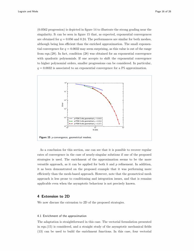
(0.0562 progression) is depicted in figure 14 to illustrate the strong grading near the

singularity. It can be seen in figure 15 that, as expected, exponential convergences

are obtained for q = 0.056 and 0.24. The performances are similar for both meshes,

although being less efficient than the enriched approximation. The small exponen-

tial convergence for q = 0.0032 may seem surprising, as this value is out of the range

from eqn.(28). In fact, condition (28) was obtained for an exponential convergence

with quadratic polynomials. If one accepts to shift the exponential convergence

to higher polynomial orders, smaller progressions can be considered. In particular,

q = 0.0032 is associated to an exponential convergence for a P5 approximation.

100 101 102

N dofs

10-5

10-4

10-3

10-2

10-1

100

Erro

r

p-FEM 2 elts geometrical q=0.0032



Figure 15 p-convergence, geometrical meshes.

As a conclusion for this section, one can see that it is possible to recover regular

rates of convergence in the case of nearly-singular solutions if one of the proposed

strategies is used. The enrichment of the approximation seems to be the more

versatile approach, as it can be applied for both h and p refinement. In addition,

it as been demonstrated on the proposed example that it was performing more

efficiently than the mesh-based approach. However, note that the geometrical mesh

approach is less prone to conditioning and integration issues, and that is remains

applicable even when the asymptotic behaviour is not precisely known.

4 Extension to 2D

We now discuss the extension to 2D of the proposed strategies.

4.1 Enrichment of the approximation

The adaptation is straightforward in this case. The vectorial formulation presented

in eqn.(15) is considered, and a straight study of the asymptotic mechanical fields

(13) can be used to build the enrichment functions. In this case, four vectorial


enrichment functions ϕi will be used:

ϕ1 = us,1r (r, θ) er + us,1

θ (r, θ) eθ

ϕ2 = us,2r (r, θ) er + us,2

θ (r, θ) eθ

ϕ3 = ub,1r (r, θ) er + ub,1

θ (r, θ) eθ

ϕ4 = ub,2r (r, θ) er + ub,2

θ (r, θ) eθ

(29)

where us,ir and ub,i

r are given in equations (30)–(33).

4.2 Geometrical mesh

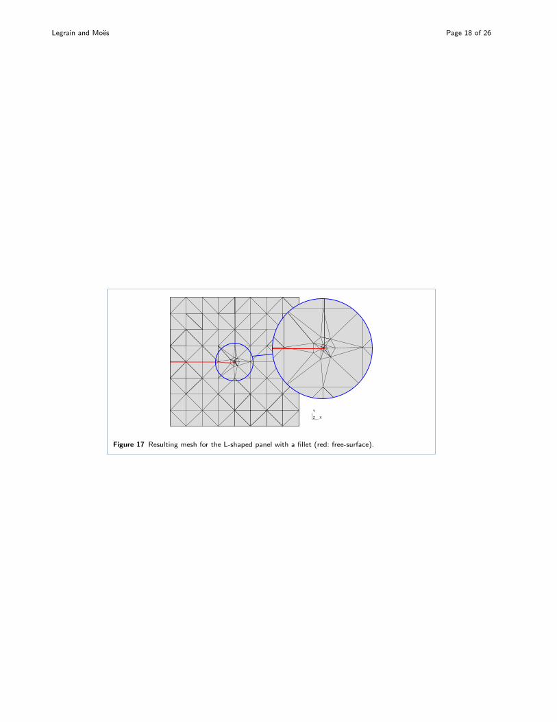
In the case of the construction of an adapted mesh, the objective is to be able to

blend a geometrical mesh into an existing finite element grid. The implementation

is easy as the computational mesh does not need to conform to the geometry,

and follows the three steps depicted in figure 16. (i) the element containing the

center of the singularity is removed from the mesh together with its neighbours.

(ii) a geometrical nodes patch is inserted in the vacant space (figure 16 b)). The

geometrical progression of this patch is obtained taking into account to the requested

number of elements made by the user, and prescribing the length of the smallest

elements to ρ (note that the value of the progression has a limited influence on

the numerical efficiency, as shown in the following). Finally (iii), a local Delaunay

algorithm is used in order to fill the space with finite elements, and build a transition

to the existing elements (figure 16 c)). An example output of this procedure is given

in figure 17. Note that the center of the progression is not the center of the radius

of curvature, but the point from which the singularity emanates (see section 1.2).

Figure 16 Blending of a geometrical into an existing grid. Note that the geometrical mesh isnon-conforming.


X

Y

Z

Figure 17 Resulting mesh for the L-shaped panel with a fillet (red: free-surface).


5 2D Numerical examples

Consider the model problem depicted in figure 18. It represents a plane domain

whose behaviour is assumed linear elastic and containing a re-entrant corner with

a fillet of radius ρ. Young’s modulus is assumed to have a unit value, and Poisson’s

ratio is 0.3. Exact tractions whose expression are given in section 1.2 are applied on

the boundaries of the domain (note that because of the geometrical approximations

used to derive the solution, exact tractions have to be applied even on the free

surface, see figure 2). In the following, ρ will range from 0.0625 to 0.1, and both h

and p-convergence are considered. In the former, only linear, quadratic and cubic

approximations will be considered. In the case where an enrichment is considered, a

“geometrical” enrichment strategy will be used by enriching all the elements lying in

a circle of fixed radius centered on the center of the singularity. In order to integrate

correctly the weak formulation in the enriched zone, the number of integration

points is simply increased in the enriched elements, but not in the remaining part

of the mesh. The objective of this section is to compare the performance of the

2D extension of the strategies considered in section 3.2, and propose good practice

rules. All the numerical examples are conducted on a geometrical domain which

consists in the bounding-box of the physical domain shown in figure 18, and the

X-FEM is used thanks to the definition of the geometry in terms of a level-set

function. A sub-grid level-set [6, 7] approach is used in order to be able to represent

the geometry accurately on coarse computational meshes. Unless mentioned, the h-

convergence studies are conducted on regular triangular meshes composed of 4× 4

to 128× 128 elements per side, and all errors correspond to relative errors.

x

y

O

Mrθ

ρ

Exacttractions

Exact tractions

Exacttractions

Exact tractions

Exact tractions

Exacttractions

2.

2.

Figure 18 Blunt re-entrant corner convergence problem.

5.1 No enrichment

In a first step, the case with no enrichment is considered with different values for ρ.

The results obtained for h-convergence, and mode I are presented in figure 19. The

behaviour highlighted in the 1D model problem is also observed here: small ρ prevent

an O(hp) convergence, especially for low polynomial orders. It can be seen that the

higher the polynomial order, the faster the convergence is recovered. The moment

when this optimal convergence is recovered is now discussed: The convergence curves

are now plotted with respect to h/ρ rather than h (see figure 20). Looking at these


curves, one can see that the change of regime in the convergence occurs in the shaded

area. This means that the asymptotic convergence is recovered for h ≃ ρ with linear

elements. Moreover, this behaviour is consistent with the theoretical previsions from

the last section (eqn. (25) for instance) Thus, the conclusion is the following: if no

enrichment is used, one should consider meshes with element of size close to ρ in

the fillet area. This condition is more easily verified when conforming low order

finite elements are used, as the construction of a conforming mesh already requires

this amount of refinement for a proper geometrical representation. This is not the

case with non-conforming methods, and p-Fem meshes using blending mapping as

elements far bigger than the radius of the fillet can be considered. When quadratic

or cubic approximations are used, the same behaviour occurs: the only difference

comes from the fact that the optimal convergence is recovered faster than in the

linear case. Yet, a very fine mesh has still to be considered (h ≃ 2 − 3 × ρ for P2

and h ≃ 3− 6× ρ for P3). In addition, optimal convergence couldn’t be recovered

in our tests for small radii.

11

21

P1 P2

3

1

P3

Figure 19 h convergence for linear, quadratic and cubic approximation with different fillet radius

Finally, p-refinement is considered with ρ = 0.00625 (smaller radius) in figure 21.

One can see that an algebraic rather than exponential convergence is obtained (as

in the 1D case).

5.2 Effect of the enrichment

The approximation is now enriched by means of the enrichment functions presented

in (29). The convergence study is done only for the smaller radius (ρ = 0.00625),


1

1

2

1

P1 P2

3

1

P3

Figure 20 Convergence regime change with respect to ρ. The shaded zone represents the zonewhere the convergence regime is changing.

mode 1 loading, and the enriched zone has a radius of 0.3. The results are presented

in figure 22. Regular convergence rates are recovered for linear, quadratic and cubic

(not shown here) approximations, even for large element size.

Next, a p-convergence is performed on 16 × 16 and 8 × 8 meshes. The enriched

zone is still a circular region of radius 0.30 and the results are given in figure 23.

Exponential convergence is recovered for both meshes with very accurate error

levels (10−4) and moderate number of dofs. Note that if the desired accuracy can

be obtained with a reasonable polynomial order (below P8), then the coarse mesh

is more efficient. Otherwise, conditioning issues with higher polynomial orders may

prevent to get a meaningful solution. In this case a finer mesh or a preconditioner

such as [21] should be used. Another alternative could be to use a non-homogeneous

p distribution (smaller p in the enriched area).

5.3 Effect of mesh refinement

Finally, the mesh-refinement strategy is evaluated. A 8× 8 base mesh is considered

(see figure 17), and 4 or 5 layers of geometrical elements are focused near the center

of the singularity (which is not the center of the radius of curvature). The results

presented in figure 24 show that an exponential convergence is obtained, and that

the number of layers has very little influence on the performances of the approach.


102 103 104 105

Dofs

10-2

10-1

100

Erro

r

p-conv ρ=0.00625, no enrichment 16×16

Figure 21 p convergence, no enrichment.

2

1

11

Figure 22 h convergence for linear, quadratic approximation with and without enrichment

5.4 Comparison of the two strategies

To conclude, the performances of the enrichment and geometrical mesh strategies

are compared for ρ = 0.00625. In the case of the use of an enrichment, the compu-

tational setup is the same as in section 5.2, whereas the number of layers is fixed

for the geometrical mesh (but 4 × 4 and 8 × 8 base meshes are considered). The

convergence curves are presented in figure 25: it is shown that the behaviour of

the different methods is quite similar, but that the enrichment strategy seems more

efficient. However, it requires the derivation of the asymptotic fields for the prob-

lem of interest. Indeed, the changing the boundary conditions on the free-surface

of the corner has an influence on the order the singularity, and the trigonometric

behaviour of the solution. On the contrary, the use of a geometrical mesh is more

versatile.


102 103 104 105

Dofs

10-5

10-4

10-3

10-2

10-1

100

Erro

r

p-conv ρ=0.00625, no enrichment 16×16p-conv ρ=0.00625, vector enrichment 16×16p-conv ρ=0.00625, vector enrichment 8×8

Figure 23 p convergence with and without enrichment, and using two different meshes.

101 102 103 104 105

Dofs

10-6

10-5

10-4

10-3

10-2

10-1

100

Erro

r

p-conv ρ=0.00625 Geometrical patch, 5 layersp-conv ρ=0.00625 Geometrical patch, 4 layersp-conv ρ=0.00625 Geometrical patch, 3 layers

Figure 24 p convergence, geometrical mesh (8× 8 base mesh).

101 102 103 104 105

Dofs

10-6

10-5

10-4

10-3

10-2

10-1

100

101

102

Erro

r

p-conv ρ=0.00625 No enrichment, 16x16p-conv ρ=0.00625 Geometrical patch, 5 layers, 8x8p-conv ρ=0.00625 Geometrical patch, 5 layers, 4x4p-conv ρ=0.00625 vector enrichment, 16x16p-conv ρ=0.00625 vector enrichment, 8x8

Figure 25 Comparison of two strategies, p convergence.


6 Conclusion

In this contribution, the behaviour of non-conforming h and p finite elements has

been studied in the case of nearly-singular solutions (re-entrant corners with a fillet

here). In particular, it has been shown in both 1D and 2D that despite being regu-

lar, the convergence rate was algebraic and limited by the order of the singularity.

Therefore, it is not possible to use fictitious domain methods such as the X-FEM

without enrichment or the Finite-Cell Method if high accuracy is needed in near

the fillet. Thanks to the study of a 1D model problem, it has been possible to

highlight the reasons for such a behaviour. Two strategies have been proposed in

order to overcome this convergence bound. The first one is based on the enrichment

of the approximation near the fillet, and is usable for both h and p methods. The

second one is based on the use of a mesh with a geometrical progression towards the

center of the singularity, and is restricted to p methods. The performances of these

two strategies have been compared in both 1D and 2D: the enrichment method is

the more efficient, but can lead to conditioning issues with high-order bases unless

proper preconditioning strategies are used [21, 23, 22, 24]. Moreover, the enrichment

function is problem dependent, and can be tedious to obtain. In the present ap-

plication, the enrichment functions are limited to stress-free bidimensional corners,

and may be not be valid in the case where Dirichlet or non-homogeneous Neumann

boundary conditions are applied. This kind of limitations was also present in the

work of Wagner et al. [29] who considered rigid particles in Stokes flow, and used

an enrichment function which is only valid for rigid and not too-close particles. The

actual improvement with such not-fully adapted enrichment functions should be in-

vestigated further. On the contrary, exponential convergence is ensured in the case

of the use of a geometrical mesh, no matter the progression, which makes it more

versatile in case of high-order methods (only). The penalty of constructing such

a mesh is greatly alleviated as this mesh does not need to conform the geometry,

which is a contribution of the paper.

Acknowledgements

The support of the ERC Advanced Grant XLS no 291102 is gratefully acknowledged

Appendix A: Asymptotic displacement fields

The asymptotic displacement fields associated to the asymptotic stress fields (4), (5), (9) and (10) are obtained by

proper integration of the strain equations. Their expressions are given below:

us,ir =

rλi

2G

[

a1(κ − λi) cos [(λi − 1)θ] − a2(κ − λi) sin [(λi − 1)θ]−

b1 cos [(λi + 1)θ] + b2 sin [(λi + 1)θ]

]

(30)

ub,ir =

rµi

2G

[

d1(κ − µi) cos [(µi − 1)θ] − d2(κ − µi) sin [(µi − 1)θ]−

c1 cos [(µi + 1)θ] + c2 sin [(µi + 1)θ]

](31)

us,i

θ =rλi

2G

[

a1(κ + λi) sin [(λi − 1)θ] + a2(κ + λi) cos [(λi − 1)θ] +

b1 sin [(λi + 1)θ] + b2 cos [(λi + 1)θ]

]

(32)

ub,i

θ =rµi

2G

[

d1(κ + µi) sin [(µi − 1)θ] + d2(κ + µi) cos [(µi − 1)θ] +

c1 sin [(µi + 1)θ] + c2 cos [(µi + 1)θ]

](33)


The expression of a1, b1, c1 as a function of a1 and b2, c2, d2 as a function of a2 are also given in [14]:

b1 =χb1(1 − λ1) a1 (34)

c1 =qλ1r

λ1−µ10

4µ1(q − 1)χc1 a1 (35)

d1 =qλ1r

λ1−µ10

4µ1(q − 1)χd1 a1 (36)

b2 = − χb2(1 − λ2) a2 (37)

c2 =qλ2r

λ2−µ20

4µ2(µ2 − 1)χc2 a2 (38)

d2 =qλ2r

λ2−µ20

4µ2(µ2 − 1)χd2 a2 (39)

References

1. Barna a. Szabo and Ivo Babuska. Finite Element Analysis. John Wiley & Sons, 1 edition, 1991.

2. Ruben Sevilla and Sonia Fern. NURBS-enhanced finite element method ( NEFEM ). International Journal for

Numerical Methods in Engineering, (February):56–83, 2008.

3. Ruben Sevilla, Sonia Fernandez-mendez, and Antonio Huerta. Comparison of high-order curved finite elements.

International Journal for Numerical Methods in Engineering, (February):719–734, 2011.

4. Nicolas Moes, John E Dolbow, and Ted Belytschko. A finite element method for crack growth without

remeshing. International Journal for Numerical Methods in Engineering, 46:131–150, 1999.

5. V K Saulev. On the solution of some boundary value problems on high performance computers by fictitious

domain method. Siberian Math. J., 4:912–925, 1963.

6. Kristell Dreau, Nicolas Chevaugeon, and Nicolas Moes. Studied X-FEM enrichment to handle material

interfaces with higher order finite element. Computer Methods in Applied Mechanics and Engineering,

199(29-32):1922–1936, 2010.

7. G. Legrain, N. Chevaugeon, and K. Dreau. High order X-FEM and levelsets for complex microstructures:

Uncoupling geometry and approximation. Computer Methods in Applied Mechanics and Engineering,

241-244:172–189, October 2012.

8. Sven Großand Arnold Reusken. An extended pressure finite element space for two-phase incompressible flows

with surface tension. Journal of Computational Physics, 224(1):40–58, May 2007.

9. A; Duster and E Rank. The p-version of the finite element method compared to an adaptive h-version for the

deformation theory of plasticity. Computer Methods in Applied Mechanics and Engineering, 190:1925–1935,

2001.

10. Gregory Legrain. A NURBS enhanced extended finite element approach for unfitted CAD analysis.

Computational Mechanics, 52(4):913–929, April 2013.

11. J M Melenk, I Babuska, and I Babuskab. The partition of unity finite element method: Basic theory and

applications. Computer Methods in Applied Mechanics and Engineering, 139:289–314, 1996.

12. M L Williams. Stress singularities resulting from various boundary conditions in angular corners of plates in

tension. ASME Journal of Applied Mechanics, 19:526–528, 1952.

13. P. Lazzarin and R. Tovo. A unified approach to the evaluation of linear elastic stress fields in the neighborhood

of cracks and notches. International Journal of Fracture, 78(1):3–19, 1996.

14. S Filippi, P. Lazzarin, and R Tovo. Developments of some explicit formulas useful to describe elastic stress fields

ahead of notches in plates. International Journal of Solids and Structures, 39(17):4543–4565, August 2002.

15. D Dini and D A Hills. Asymptotic characterisation of nearly-sharp notch root stress fields. International Journal

of Fracture, 130(3):651–666, December 2004.

16. M. Creager and P.C. Paris. Elastic field equations for blunt cracks with reference to stress corrosion cracking.

International Journal of Fracture Mechanics, 3(4):247–252, 1967.

17. G. Glinka. Calculation of inelastic notch-tip strain- stress histories under cyclic loading. Engineering Fracture

Mechanics, 22(5):839–854, 1985.

18. N. Sukumar, D. L. Chopp, Nicolas Moes, and Ted Belytschko. Modeling Holes and Inclusions by Level Sets in

the Extended Finite Element Method. Comp. Meth. in Applied Mech. and Engrg., 190:6183–6200, 2001.

19. W. D. Lian, Gregory Legrain, and P. Cartraud. Image-based computational homogenization and localization:

comparison between X-FEM/levelset and voxel-based approaches. Computational Mechanics, May 2012.

20. Gregory Legrain, R Allais, and Patrice Cartraud. On the use of the extended finite element method with

quadtree/octree meshes. International Journal for Numerical Methods in Engineering, (December

2010):717–743, 2011.

21. Eric Bechet, H Minnebo, Nicolas Moes, and B Burgardt. Improved implementation and robustness study of the

X-FEM for stress analysis around cracks. International Journal for Numerical Methods in Engineering,

64(8):1033–1056, 2005.

22. Patrick Laborde, J Pommier, Yves Renard, and Michel Salaun. High-order extended finite element method for

cracked domains. International Journal for Numerical Methods in Engineering, 64(3):354–381, 2005.

23. Uday Banerjee and John E Osborn. Generalized Finite Element Methods: Main Ideas, Results, and Perspective.

Technical report.

24. Marcel Ndeffo, Patrick Massin, and Nicolas Moes. Crack Propagation Modelisation Using XFEM With 2D and

3D Quadratic Elements. In International Conference on Extended Finite Element Methods – XFEM 2013, 2013.


25. C.Armando A. Duarte, Ivo Babuska, and J.Tinsley Tinsley Oden. Generalized Finite element methods for

three-dimensional structural mechanics problems. Computers and structures, 77:215–232, 2000.

26. Nicolas Chevaugeon, Nicolas Moes, and Hans Minnebo. Improved Crack Tip Enrichment Functions and

Integration for Crack Modeling Using the Extended Finite Element Method. International Journal for Multiscale

Computational Engineering, 11(6):597–631, 2013.

27. I. Babuska and B. Guo. The h, p and h-p version of the finite element method; basis theory and applications.

Advances in Engineering Software, 15:159–174, 1992.

28. W Gui and Ivo Babuska. The p andh-p versions of the finite element method in 1 dimension. Part I: The basic

approximation results. Numerische Mathematik, 612:577–612, 1986.

29. G J Wagner, Nicolas Moes, W K Liu, and Ted Belytschko. The Extended Finite Element Method for Stokes

Flow Past Rigid Cylinders. International Journal for Numerical Methods in Engineering, 51:293–313, 2001.

treatment of nearly-singular problems with the x-fem

Documents